the assembly of multiple form structures

Preliminary Version Equation Chapter 1 Section 1

Ronald Armstrong & Jennifer Little Rutgers Business School Newark/New Brunswick

Rutgers University Corresponding author: Ronald D. Armstrong Management Science & Information Systems Rutgers University 180 University Avenue

Newark, NJ 07102-1895

[email protected]

Paper presented at the 2003annual meeting of NCME, Chicago, IL, April, 2003.

This research has been funded by a grant from the Law School Admission Council.

April 15, 2003

The Assembly of Multiple Form Structures

Assembly of Multiple Form Structures

2

ABSTRACT


A multiple-form structure (MFS) is an ordered collection of testlets. A test-taker’s

progression through the network of testlets adapts to the test-taker’s ability. The collection of

paths through the network yields the set of all possible test forms. This paper presents mixed

integer programming models for MFS assembly problems. Test specifications are placed on

every path of the MFS. The models consider single MFS assembly and sequential MFS

assembly. Computational results with commercial optimization software will be given and

advantages of the models evaluated.


Executive Summary

The last decade has seen paper-and-pencil (P&P) tests being replaced by computerized

adaptive tests (CATs) within many testing programs. A CAT may yield several advantages

relative to a conventional P&P test. A CAT can determine the items to administer in real time,

allowing each test form to be tailored to a test-taker’s skill level. That is, a test-taker’s responses

to items can be assessed sequentially during the test and a regularly updated estimate of the test-

taker’s ability can be maintained. Subsequent items can be chosen to more closely match the

capability of the test-taker. By adapting to a test-taker’s ability, a CAT can acquire more

information about a test-taker while administering fewer items.

A multiple form structure (MFS) provides a means to implement a CAT that allows

review before the administration. An MFS is an ordered collection of testlets. Every test-taker is

administered the same testlet(s) early in the test, but the choice of later testlets is dependent on an

assessment of ability. The MFS format is a hybrid between the conventional P&P and CAT

formats. The possible paths through the MFS give the possible test forms for the MFS. Every

form must satisfy its own test specifications.

This paper presents mixed integer programming models for MFS assembly problems.

Both discrete item types and set based item types are considered. Certain models rely heavily on

network flow techniques. The underlying network flow structure enhances the convergence of

the branch and cut algorithm used to solve the problems. Computational results are reported

with a commercial mixed integer programming software package. The models consider a single

MFS assembly, sequential MFS assembly and simultaneous compound MFS assembly.

Computational results with commercial optimization software will be given and advantages of

the models evaluated.


2


Introduction

A multiple form structure (MFS) provides a means to implement a computerized

adaptive test (CAT) that may reduce certain CAT deficiencies. An MFS is an ordered

collection of testlets (Wainer and Kiely, 1987) that allows for adaptation based on a test-

taker’s ability while exposing a pre-set number of items. This test structure is a hybrid

between the conventional paper-and-pencil (P&P) test and a CAT. It is a computerized

extension of the early attempts at adaptive tests by Lord (1971), where multiple-stage

tests were given and the tests to give at later stages depended on performance in earlier

stages. Partly because the computer was not used, Lord had two stages with an extended

time period between stages.

A Multiple Form Structure Design (MFSD) is a framework for a class of MFSs;

that is, an MFSD has no items or testlets associated with it. An MFSD gives the position

of bins designed for a test-taker classification, and a testlet is placed in each bin to create

an MFS. The sequences of bins a test-taker may follow yields the paths through the

MFS. The combined testlets on a path yields a test form of the MFS. The MFSD also

states the constraints for every path. This paper introduces models to assemble MFSs

from an MFSD. All MFSs assembled for an MFSD are considered parallel to one

another, as standardized linear test forms are considered parallel to each other.

The use of mathematical programming techniques to assemble test forms is

common at testing agencies. These techniques save hundreds of hours of personnel time.

A test form assembled by a computer can be assured to satisfy all test specifications.

While the review of the form by test specialists may still be desirable, the review

generally entails a small number of alterations to account for constraints not coded in the

database. The more notable heuristic methods for test assembly are Luecht and Hirsch

(1992), Luecht (1998), and Stocking and Swanson (1993). Armstrong, Jones and Kunce

(1998) and Armstrong, Jones and Wu (1992) utilize network flow and Lagrangian

relaxation for test assembly. Theunissen (1985), van der Linden (1998), and van der

Linden (2000) propose the use of a more general mixed integer programming


3

(Nemhauser and Wolsey, 1988) software package. This paper takes the last approach and

uses a commercially available code, CPLEX (ILOG, 1999), as the tool to obtain solutions

to mixed integer programming problems arising from the MFS assembly models. The

process to be presented can be implemented with any software package that could solve

large-scale mixed integer programming (MIP) problems.

The next section gives an example of an MFSD and demonstrates how it can be

represented with a tree structure. The next two sections present generic models that can

be used with mixed integer programming software to assemble an MFS. The first of

these sections gives models for discrete items and the subsequent section gives models

for set based items. The fundamental models are extended to generalized network

formulations. Computational results are given after the models are presented. The

concluding section discusses extensions to the models and how the assembly might take

place in an operational setting.

Example of an MFSD

MFSDs differ in the number of bins, number of items per bin, the number of

stages, the target curves and the constraints. All MFSs corresponding to a particular

MFSD will be similar in all of these attributes. Figure 1 depicts an example of an MFSD

that is being evaluated. The layout depicts an MFSD having six stages with a total of

twelve bins. The bins at a given stage are arranged in levels corresponding to item

difficulty/test-taker ability classifications or strata. In this example, every MFS bin will

be assigned a testlet with five, six or seven items. Every possible path through the MFS

constitutes a test form, and each path has between 35 and 37 items. The path that a

particular test-taker may traverse through an MFS contains exactly one testlet from each

stage. More flexible designs can be developed where the administration can be

terminated based the confidence interval of an ability estimate; but this is not considered

here.

(insert Figure 1 about here)

The convention used for numbering the bins is sequential starting at the first

stage. The numbering within a stage has the bin designed for the lowest ability given the

smallest index. Similarly, the paths are numbered with path 1 containing the bins with


4

the smallest indices in the stages, and the highest numbered path has the largest bin

indices in the stages.

The design of Figure 1 either has an automatic routing after a bin or binary

routing decision is made after a bin. There are four paths for this particular MFSD. The

MFSD can be depicted as a tree as shown in Figure 2. For the MFSD of Figure 1, bins 10

and 11 can be arrived at by traversing different paths; thus, two nodes appear in the tree

for both bins 10 and 11. A routing decision must be made at each point in the tree where

a split takes place. The routing rules are not used directly for the MFS assembly

problem. However, the routing is important when obtaining the target information

functions and target characteristic curves for a path, as these targets are aimed at the

group of test-takers traversing the path. Also, the routing rules and targets can be used to

estimate the probability of a test-taker with a given ability traversing a path. Armstrong

and Roussos (2002) describe a method to create targets for each bin, and the bin targets

are used to create path targets.


The items used in the assembly are calibrated with a single ability 3-parameter

item response (IRT) model. Given the parameters, the information and probability of a

correct response for an item can be calculated at an ability level. It is assumed that the

items are independent; thus, information and correct response probabilities can be added

to obtain the corresponding overall (conditional) information and expected score for

multiple items. The MFS approach to testing can be extended to classical or other IRT

models.

The MFSDs considered in this study are evaluated for a possible implementation

of the Law School Admission Test (LSAT). The LSAT is currently given in a linear

paper and pencil (P&P) format. Modification to the models may be necessary for other

tests. However, the LSAT is representative of most tests and the results of this paper can

be applied outside of the LSAT.

Generic MFS Assembly Model – Discrete Item Case An item is discrete if the item’s stimulus and question can be treated as a unit.

This segment considers the problem of assembling a single MFS where all the items


5

eligible to be assigned are multiple choice and discrete. The generic model considers the

following constraints for MFS assembly.

• Testlet to bin assignment. Each bin must have exactly one testlet assigned to it.

• Single occurrence. An item can appear at most once on a path (form).

• Testlet size. There is a range on the number of items in the testlet assigned to a bin.

• Targets. Each path has target information functions and target characteristic curves. The information function and characteristic curves for the paths must be within a specified range of the targets.

• Cognitive skill content. A distribution of the cognitive skills being tested must be satisfied over each path. The cognitive skills constraints uses in this study are an extrapolation of those for the current LSAT P&P linear test.

Most of the MFSDs have a sequence of two bins where the routing of the test-

taker from one bin to the next is automatic. This is done to keep the structure simple, and

there is little improvement in scoring accuracy by making a routing decision after each

testlet. When the automatic routing takes place, the testlets assigned to the two bins

could be combined into one larger testlet. This is not done because a testlet having more

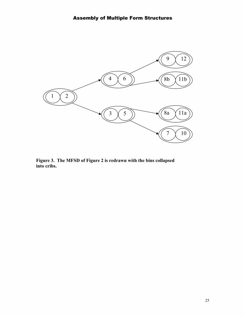
than 10 items becomes difficult to manage for the test-taker. A crib is a sequence of bins

where the only routing decision takes place after the administering the testlet from the

last bin in the sequence. The MFS assembly problem considered here assigns items to

cribs, and the separation of the items into the bins takes place later. Figure 3 gives the

tree representation of an MFSD with cribs.


The following notation is defined before the statement of the models.

N - The number of items in the pool eligible to appear on the MFS is denoted by N .

The items are indexed 1,2,...,i N= .

M - The number of cribs in the MFSD is denoted by M . The cribs are indexed

1,2,...,j M= .

Π - The number of paths in the MFSD. The paths are indexed 1,2,...,π = Π .

( )B π - The index set of cribs on path π , 1, 2,...,π = Π .


6

ujn and d

jn - The upper and lower limits on the number of items to be assigned to crib

j , 1, 2,...,j M= .

G - The number of cognitive skills content constraints on each path. It is assumed

that each path has the same cognitive skill content requirements, although this

is not required by the model.

ugr and d

gr - The upper and lower limits on the number of items on a path testing

cognitive skill g , 1, 2,...,g G= . The first cognitive skill is tested by every

item eligible to be assigned to the MFS; thus, the total number of items on a

path must be in the interval 1 1[ , ]d ur r .

gR - The index set of all items testing cognitive skill g , 1, 2,...,g G= . The index set

1 {1,..., }R N= is the index set of all items eligible for assignment to the MFS.

K - The number of points on the ability axis where upper and lower limits are

specified for the test information function and test characteristic curve. These

points are denoted by , 1,2,...,k k Kθ = .

( )i kI θ - The information provided by item i at , 1,...,k i Nθ = and 1,2,...,k K= .

Independence of items is assumed.

( )i kP θ - The probability of a correct response on item i by a test-taker with ability

, 1,...,k i Nθ = and 1,2,...,k K= .

( )ukTIFπ θ and ( )d

kTIFπ θ - The upper and lower limits on the test information

function on path π evaluated at , 1,2,...,k k Kθ = .

( )ukTCCπ θ and ( )d

kTCCπ θ - The upper and lower limits on the test characteristic

curve on path π evaluated at , 1,2,...,k k Kθ = .

The constraints for the generic MFS assembly problem with discrete items are the

following.


7

1

1 , 1,...,N

uij j j

i

x s n j M=

+ = =∑ ; (1)

0 1 , 1,...,u dj j js n n j M≤ ≤ − = ; (2)

( )1, 1,..., , 1,...,ij

j B

x i Nπ

π∈

≤ = = Π∑ ; (3)

( )2 , 1,..., , 1,...,

g

uij g g

i R j B

x s r g Gπ

π∈ ∈

+ = = Π =∑ ∑ ; (4)

0 2 , 1,..., ;u dg g gs r r g G≤ ≤ − = (5)

( )( )

( )1

3 , 1,..., , 1,....,N

ui k ij k k

j L i

I x s TIF k Kπ ππ

θ θ π∈ =

+ = = Π =∑ ∑ ; (6)

( ) ( )0 3 , 1,..., , 1,....,u dk k ks TIF TIF k Kπ π πθ θ π≤ ≤ − = Π = ; (7)

( )( )

( )1

4 , 1,..., , 1,....,N

ui k ij k k

j B i

P x s TCC k Kπ ππ

θ θ π∈ =

+ = = Π =∑ ∑ ; (8)

( ) ( )0 4 , 1,..., , 1,....,u dk k ks TCC TCC k Kπ π πθ θ π≤ ≤ − = Π = ; (9)

ijx = 0 or 1, 1,..., , 1,..., .i N j M= = (10)

The decision variable ijx equals 1 if item i is assigned to crib j , and equals 0

otherwise. Constraint (10) assures this binary restriction. Constraints (1) and (2) assure

that between djn and u

jn items are assigned to crib j . If the MFSD has djn = u

jn , the

slack 1 js and the constraint from (2) are omitted. As observed before, after the MFS

assembly, post-processing must be used to distribute the items from the crib to the

associated bins. Constraint (3) assures that an item can appear at most once on a path.

Constraints (4) and (5) assure the satisfaction of the cognitive skill distribution

constraints on each path. The slack, 2gs , is not necessary when d ug gr r= . Constraints (7)

through (10) assure that each path information function and path characteristic curve falls

within an interval about the targets.


8

Objective Function.

Various objective functions could be considered. A commonly used objective for

linear tests is to minimize the distance the test information function and characteristic

curve are from the middle of the lower and upper acceptable limits. Minimizing the sum

of the absolute deviations and minimizing the maximum absolute deviation both give rise

to linear objective functions. CPLEX does have a capability to solve MIPs with a

quadratic objective functions; therefore, the squared deviation could be considered.

However, any solution to the constraints yields an acceptable test in terms of the test

specifications. The purpose of this study is to produce many MFSs that meet the

specifications. The objective function used in the following analysis assigns random

costs to the items. The objective function is the following.

1 1

N M

i iji j

Minimize c x= =∑∑ (11)

The cost ic is the same for all item assignments. This is done to encourage the

allocation of an item multiple times in an MFS. If an item has a low cost, enhancing the

chances of its assignment, it is more likely to be assigned to two or more cribs on

different paths than if each assignment has its own random cost.

While this problem may be solved in its present form, it always helpful to

consider alternative and potentially “better” formulations without changing the

acceptability of a solution. The first adjustment removes constraints that are almost

irrelevant, and the second attempts to restructure the constraints in a representation to

speed the convergence of the branch-and-cut method employed by CPLEX.

Reduction of the Target Constraints.

The target information and expected score constraints are defined over a wide

ability range – in the current study, from -3.0 to +3.0 in steps of 0.3. There is an

extremely small probability that test-takers with certain abilities will follow a given path.

For example, a test-taker with an ability of -2.0 will almost never follow the path

intended for the highest ability group. An estimate of the probability of a test-taker

traversing a path, conditioned on ability, can be calculated as described in Armstrong


9

(2002) and Armstrong and Roussos (2002). If this estimated probability is small, the

associated target constraint can be omitted without noticeable loss of parallelism.

The probability of a test-taker with a given ability, θ , traversing a path has a

single mode. The highest (lowest) numbered path will have the probability peak at

Kθ θ= ( 0θ θ= ). The other paths will have the probability peak at an ability point

between 0θ and Kθ . Let dKπ and uKπ be the first and last quadrature point considered for

the target restrictions on path π , respectively. Constraint sets (6) through (9) can be

rewritten considering only the quadrature points between dKπ and uKπ , inclusive.

Generalized Network Formulation.

Most of the constraints of the generic model can be represented with a generalized

network flow model (Ahuja, Magananti and Orlin, 1996). This is important because the

convergence of branch and cut algorithms generally will be enhanced by the presence of

the network (Williams, 1990). The only constraints of the generic problem that cannot be

represented in the network are the target constraints. The network formulation does not

decrease the number of variables or constraints, but makes the continuous problem more

representative of the MIP problem. The branch-and-cut MIP solution methods, such as

used by CPLEX, start with the integer restrictions relaxed and work toward an integer

solution.

Every arc in the network connects two nodes, and flow is directed from a tail

node to a head node. The mathematical programming model has a decision variable for

each arc and a constraint for each node. For arc ( ,t h ), let thc represent a cost per unit,

thlow and thcap represent the lower and upper limits on the flow, and thβ represent the

arc multiplier. Let thv represent the amount of flow from node t . The flow arriving at

node h is th thvβ . The networks considered here have integer flow. A generalized

network mathematical programming model will have exactly two non-zero entries in

every column. One entry will be a +1 and the other entry will be negative. If all the

negative numbers are equal to -1, then the model is a pure network flow model. The

model presented here is a generalized network flow model with additional constraints.


10

The degree-out of node t is the number of arcs who have node t as a tail. The

degree- in of node h is the number of arcs who have node h as a head. Denote all the arcs

in the network by ARCS and all the nodes in the network by ND . Define ( )T h =

{ ( , ) }t t h ARCS∈ and ( )H t = { ( , ) }h t h ARCS∈ . The network flow models of this paper

have the multiplier on arc ( ,t h ) equal to the degree out of node h, unless the degree out is

zero, in which case, the multiplier is one.

The nodes of the network, ND , are separated into distinct groups. These groups

are connected with arcs. The item supply nodes have a degree-in of zero and positive

supply. There are nodes for the MFS networks and nodes for the cognitive skills

distribution. These are pure transshipment nodes; that is, all the flow arriving at a node

leaves the node. There is a special node denoted as the sink. The sink receives all the

flow through the network. The sink is designated as node 0 and has a degree out of zero.

Item Supply Network The items are considered a commodity that is shipped to the MFS. The item

supply network structure creates one node for each crib. Let 1ND represent the index set

of the item supply nodes. Since the generic model can assign any item to any crib, each

item has one associated arc out of each item supply node. The supply at a node is equal

to the upper limit on the number of items that can be shipped to the corresponding crib

( ujn ). Arcs directed from the item supply nodes to the MFS network assure no more than

ujn items are assigned to crib j . An arc connecting each item supply node to the sink has

capacity u dj jn n− assuring at least d

jn items will be sent to the MFS network.

Let ( , )i t h denote the item index associated with arc ( , )t h where node 1t ND∈ .

The flow over these arcs must be one or zero, indicating whether or not an item is

assigned to a specific crib. Both the tail node, t , and the head node, h , are designation

as nodes associated with a crib. The tail is a crib node in the item supply network and the

head is a crib node in the MFS network to be discussed next.

MFS Network


11

The MFS tree structure is the foundation of an MFS network. An example of the

tree is given in Figure 3 where the MFS of Figure 2 with bins as the nodes is replaced by

the cribs as nodes. The tree structure needs to be modified to assign the items to the cribs

that appear on more than one path. An intermediate node is needed for every crib

represented by more than one node in the tree. This node distributes an item to each of

the nodes representing the crib. Each item has its own MFS network and the MFS

networks are identical in structure. The capacity of every arc entering an MFS network

and every arc leaving an MFS network has a capacity of one and lower flow limit of zero.

Figure 4 outlines an MFS network for the MFSD of Figure 1. Let ND2 represent the

nodes of the MFS networks for all items.


Once a unit of flow (an item assignment) enters an MFS network, the flow

through the remainder of the network is mandated. The zero or one flow restrictions are

needed only for the arcs connecting ND1 to ND2. The multiplier for an arc is equal to

the degree out of the head node. The capacity of every arc in an MFS network is one.

The MFS network automatically enforces the requirement that an item can appear on a

path at most once.

The end node of an MFS network (see Figure 4) represents the final crib on an

MFS path. A single arc leaves each end node and flow over the arc is one or zero,

indicating whether or not an item is assigned to a crib on a specific path. Both the tail

node, t , and the head node, h , are designation as nodes associated with a path. The tail

is a terminal node in an MFS network and the head is a node in the cognitive skills

network to be discussed next.

Cognitive Skills Network The cognitive skills distribution for a single path can be represented in a

hierarchical manner for all of the MFSDs of this study. This means that they can be

represented as pure network flow constraints. The set of constraints relating to cognitive

skills distribution are broken down into levels, the highest level corresponding to the

most detailed item classification. Level 1 is the most general level and this cognitive skill

is tested by every item eligible to be placed on the MFS. The number of nodes is G - the


12

number of cognitive skills constraints. Each item is identified as belonging to class

according to the most detailed level. An item belongs to a single cognitive skills class.

The cognitive skills network for a single path has a tree structure with the nodes

with a degree-in of zero at the highest level and the root node level 1. As the level of the

tree decreases, item classifications at the highest level merge to create the groupings at

the current level. Each node restricts the number of items from the node’s associated

cognitive skills constraint through specification of an upper and a lower limit on the arc

flowing from the node. Figure 5 shows a possible cognitive skills network for a single

path. It is assumed that the cognitive skills constraints are the same for each path; thus,

this tree network is duplicated for each path. Let ND3 denote the nodes in the cognitive

skills networks for all paths, and 3( )ND g denote a node for cognitive skill constraint g .


Let ( , )i t h denote the item index associated with arc ( , )t h where node 2t ND∈

and 3h ND∈ , as discussed at the end of the previous subsection. Both t and h are

designated as nodes associated with a path. The tail is a node in the MFS network at the

end of a path, and the head is the node associated with the most detailed cognitive skills

classification for the item within the path’s cognitive skills network. Let ( , )path t h

denote the path associated with arc ( , )t h and ( , )i t h denote the associated item index.

The root node for each tree of the cognitive skills network is the node that collects

the flow from all of the items on the associated path. The number of items on a path may

not be fixed; that is, 1ur may be greater than 1

dr . An arc is created from the root node to

the sink with the thlow = 1dr and thcap = 1

ur .

Generalized Network Model Statement The generalized network has an item supply network, MFS networks (one for

each item), cognitive skills networks (one for each path) and a sink node. The item

supply network has the only nodes with a positive supply. All other nodes in the

network, except for the sink, have a zero demand and flow passes through these nodes.

There are arcs connecting the item supply network to the MFS network. These arcs and

all arcs in the MFS network have multipliers equal to the degree-out of the head node.


13

The capacities for arcs connecting the MFS network have capacity of 1 and lower flow

limit of zero. The network automatically enforces the constraints that an item can appear

at most once on a path, the constraints on the number of items to be assigned to a crib and

the cognitive skills constraints.

Let thv represent the flow from node t to node h. The generalized network flow

statement of the generic MFS model for the discrete item case is the following.

( , )1, 2

i t h tht ND h ND

Minimize c v∈ ∈∑ (12)

( )

, 1;uth t

h H t

v n t ND∈

= ∈∑ (13)

00 , 1;u dt t tv n n t ND≤ ≤ − ∈ (14)

thv = 0 or 1, 1t ND∈ and 2h ND∈ (15)

( ) ( )0ht th th

t H h t T hv vβ

∈ ∈

− =∑ ∑ 1, 0h ND h∉ ≠ ; (16)

0 1thv≤ ≤ 3, 0t ND h∉ ≠ ; (17)

d ug th gr v r≤ ≤ where 3( )t ND g= (18)

0(0)

0tt T

v∈

− ≤∑ (19)

( )( , )( , ) ,

3

( ) 3 , 1,..., , ,....,u d ui t h k th k k

path t hh ND

I v s TIF k K Kπ π π ππ

θ θ π=

∈

+ = = Π =∑ ; (20)

( ) ( )0 3 , 1,..., , ,....,u d d uk k ks TIF TIF k K Kπ π π π πθ θ π≤ ≤ − = Π = ; (21)

( )( , )( , ) ,

3

( ) 4 , 1,..., , ,....,u d ui t h k th k k

path t hh ND

P v s TCC k K Kπ π π ππ

θ θ π=

∈

+ = = Π =∑ ; (22)

( ) ( )0 4 , 1,..., , ,....,u d d uk k ks TCC TCC k K Kπ π π π πθ θ π≤ ≤ − = Π = ; (23)


14

Constraints (13) and (14) assure the assignment of between dtn and u

tn items to

each crib, as there is one node in 1ND for each crib. Constraint (15) requires an item to

be assigned to a crib or not. Constraint set (16) conserves the flow in the network for all

nodes in 2ND and 3ND . The flow on all arcs leaving node h is equal to flow on all

arcs entering node h times the respective arc multiplier. Constraint set (18) forces the

satisfaction of cognitive skill requirements. Constraint (19) allows the sink node to

absorb all flow passing through the network.

Generic MFS Assembly Model – Set Based Item Case An item is set based if the item’s stimulus is used as the stimulus for multiple

items. This segment considers the problem of assembling a single MFS where all the

items eligible to be assigned are multiple choice and set based. The stimulus and the

associated items create the testlet for the MFS. All the constraints for the discrete item

case are still applicable. The new constraints for the generic model are the following.

• Single occurrence. A stimulus can appear at most once on a path (form).

• Stimulus to bin assignment. There must be exactly one stimulus assigned to each bin.

• Item set usage. When a stimulus is assigned to a form, an upper bound and a lower bound on the total number of items from the associated item set is required.

• Priority items in the set. There may be a subset of items within the item set where at least one item from the subset must appear in the MFS when the associated stimulus is assigned to a form.

• Topic specifications. The stimuli for set based items are categorized according to general topics. Every stimulus has a single general topic; for example, “science” might be a topic. Each MFS must have a specified number of stimuli of each topic.

The first and second constraints stated above replace constraints (1) and (2)

(constraints (13) and (14) from the network model). To state the model for the set based

case, some new notation is necessary.

L - The number of stimuli in the pool is denoted by L .

jm - The number of stimuli that must be assigned to crib j is jm . For all the

MFSDs considered in this study, jm equals 1 or 2.

( )I - The index set of items whose stimulus is indexed by .


15

( )I ′ - The subset of items contained in ( )I where at least one of the items from

this subset must appear on an MFS if stimulus appears. The set ( )I ′ may

be empty.

dλ and uλ - The lower and upper limit on the number of items from set that must

appear on the MFS if stimulus appears.

Q - The number of distinct topics is denoted by Q .

dqτ and u

qτ - The lower and upper limit on the number of stimuli of topic q appearing

on a path of the MFS.

( )L q - The index set of those stimuli in the pool having topic q .

The new constraints to be added to the generic model for the discrete item case

are the following.

( )

1, 1,..., , 1,..., ;jj B

y Lπ

π∈

≤ = = Π∑ (24)

1

, 1,...,L

j jy m j M=

= =∑ ; (25)

( )

5 0, 1,..., , 1,..., ;uij j j

i I

x y s L j Mλ∈

− + = = =∑ (26)

0 5 , 1,..., , 1,..., ;u djs L j Mλ λ≤ ≤ − = = (27)

( )

0,j iji I

y x′∈

− ≤ ∀∑ where ( )I ′ ≠ empty set and 1,...,j M= ; (28)

( ) ( )

6 , 1,..., 1,..., ;dj q q

L q j B

y s q Qππ

τ π∈ ∈

+ = = = Π∑ ∑ (29)

0 6 , 1,..., ;u dq q qs q Qπ τ τ≤ ≤ − = (30)

0 1, 1,..., 1,..., ;jy or L j M= = = (31)

The decision variable jy equals 1 if stimulus is assigned to crib j , and equals

0 otherwise. This is enforced by constraint set (31). The assignment of the correct


16

number of stimuli to each crib is given by (25). The item set usage constraints are given

by (26) and (27). The required usage of at least one priority item is given by (28). The

topic distribution is enforced by constraint sets (29) and (30). If u dq qτ τ= , the slack

variable 6qs π can be omitted. The constraints (3) through (10) remain in the model.

Objective Function.

As was the case with the discrete item model, the purpose of the study was to

produce many MFSs that meet the specifications. The objective function used in the

following analysis assigns random costs to the stimuli and its items. The objective

function is the following.

1 ( ) 1

L N M

iji I j

Minimize c c x= ∈ =

+∑ ∑ ∑ (32)

The cost c is the same for all assignments for a stimulus and all items in the item

set. This is done to encourage the allocation of an item or stimulus multiple times in an

MFS. A low cost enhances the chances of the assignment of the stimulus and its items to

an MFS.

Generalized Network Formulation.

The generalized network flow model for the set based items is similar to the one

for the discrete items. Some nodes of the network will be fixed-charge nodes; that is,

these nodes have a positive supply greater than one or a supply of zero depending on

whether or not a fixed charge is incurred.

Stimulus Supply Network The stimulus supply network is based directly on the item supply network for the

discrete case. There is one node for each crib and the supply is jm where the index j

gives the crib associated with the node. As noted previously, for all the MFSDs

considered in this study, jm equals 1 or 2. There are no arcs to the sink as the number of

stimuli, jm , to assign to a crib fixed. Arcs connect the stimulus supply nodes to an MFS

network for each stimulus. These arcs are restricted to a flow of zero or one.


17

Item Supply Network The nodes of the item supply network are fixed-charge nodes. There is one item

supply network for each stimulus. These nodes correspond to the cribs of the MFSD.

The nodes have a supply only when the associated stimulus is assigned to the associated

crib. For each node t in the items supply network, let ( )t denote the stimulus

associated with the node and ( )j t denote the crib associated with the node; therefore,

node t has a positive supply only when stimulus ( )t is assigned to crib ( )j t . The

following description of the item supply network does not repeatedly condition the

existence of supply at a node on the stimulus/crib assignment.

Let 1ND represent the index set of the item supply nodes. The set 1ND is

divided into two subsets. The first subset, denoted by 1ND ′ , has the supply for the

priority items of the stimulus. This supply is the cardinality of the set ( )I ′ , denoted by

( )I ′ . The second subset, denoted by ND′′ , has the supply for the non-priority items.

This supply is ( )u Iλ ′− . If ( )I ′ >1, not all the supply at the associated node in

1ND ′ need to used. In this case, an arc connects node 1t ND ′∈ to node 2h ND ′′∈ where

( ) ( )t h= and ( ) ( )j t j h= . The capacity of the arc is ( )I ′ -1.

There may be unused supply at node 1t ND ′′∈ . If stimulus ( )t is assigned to a

crib, a minimum of dλ items must be used. The unused supply is sent to the sink. Every

node 1t ND ′′∈ has an arc ( ,0)t with a capacity of ( ) ( )u dl t tλ λ− .

An arc connects every node of the item supply network to the associated crib node

in the MFS network. As before, there is one item supply network for each item.

MFS Network and Cognitive Skills Network The construction of the MFS Network and Cognitive Skills Network are identical

to the construction described for the discrete item case. The stimulus supply nodes are

connected to an MFS network in exactly the same manner as the item supply nodes of the

discrete model were connected. Connecting the stimulus supply network with an MFS

network assures a stimulus is used on at most one path. The terminal nodes associated

with an MFS network correspond to the terminal cribs for a path of the MFS. Each


18

terminal node for a stimulus MFS network connects to a node in a topic network to be

described next.

Topic Network There are no cognitive skills restrictions on the stimuli of a path. There is a topic

restriction, and a topic network enforces coverage. There is one topic network for each

path. Unlike the cognitive skills network, there is only one level for the topic network;

thus, no arcs connects nodes within a topic network. Topic network nodes are pure

transshipment nodes, and there is a single arc out of each node connecting to the sink.

These arcs have 0tlow = dqτ and 0tcap = u

qτ . Let ( ,0)path t denote the path associated with

arc ( ,0)t and ( ,0)topic t denote the associated topic.

Generalized Network Model Statement The generalized network has stimulus supply networks, item supply networks

(one for each stimulus), MFS networks (one for each item and one for each stimulus),

cognitive skills networks (one for each path), topic networks (one for each path) and a

sink node. The stimulus supply networks have the only nodes with a positive supply.

The supply at an item supply network node is a fixed-charge supply; that is, it has supply

only if the associated stimulus to crib assigned is made. All other nodes in the network,

except for the sink, have a zero demand and flow passes through these nodes. There are

arcs connecting an item supply network to an MFS network. These arcs and all arcs in a

MFS network have multipliers equal to the degree-out of the head node. The capacities

for arcs connecting a MFS network have capacity of 1 and lower flow limit of zero. The

network automatically enforces the constraints that an item and stimulus can appear at

most once on a path, the constraints on the number of items to be assigned to a crib, the

cognitive skills constraints and the topic distribution constraints. Let thw represent the

arc flows associated with a stimulus. The generic generalized fixed-charge network flow

model for set based items is the following.

( , ) ( , )0, 2 1, 2

t h th t h tht ND h ND t ND h ND

Minimize c w c v∈ ∈ ∈ ∈

+∑ ∑ (33)

subject to


19

( )

, 0;th th J t

w m t ND∈

= ∀ ∈∑ (34)

thw = 0 or 1, 0;t ND∀ ∈ (35)

( ) ( )

0ht th tht H h t T h

w wβ∈ ∈

− =∑ ∑ 0,h ≠ ; (36)

0 1 0thw h≤ ≤ ≠ and 0d uq t qwτ τ≤ ≤ , ( ,0)topic t q= (37)

( )

( ( , )) 0, 1 ;th thh J t

v I t h w t ND∈

′ ′− = ∀ ∈∑ (38)

0 ( ( , )) 1 1 , 1 ;thv I t h t ND h ND′ ′ ′′≤ ≤ − ∈ ∈ (39)

( , )( )

( ( ( , )) ) 0, 1 ;uth t h th

h J t

v I t h w t NDλ∈

′ ′′− − = ∀ ∈∑ (40)

0 ( ) ( )0 1 ;u dt l t tv t NDλ λ ′′≤ ≤ − ∈ (41)

Constraints (15) through (23) are needed to complete the model.

Computational Results Limited computational results can be reported at this time. Initial results indicate

the benefits of the network flow models, but further study is necessary before definitive

statements can be made. The results reported here are for the network flow model. All

solution times were the results of runs on a desktop personal computer with a Pentium 4

CPU, 2.00 GHz, 1.00GB of RAM, and Windows XP operating system. The item pool

was saved in a Microsoft Access database. All MIP problems were solved with CPLEX

(ILOG, 1999). All programs extracting data from the database, constructing the input to

CPLEX, and writing the results to the database were written in C/C++ by the authors.

The programs interfaced directly with the CPLEX library.

Table 1 shows the results from the solution of MFSs from the MFSD of Figure 1.

The pool had 1336 items. The MFSD had 6 cribs, 4 paths, 20 cognitive skill distribution

constraints per path and 21 ability points for targets constraints per path. The relative

width of the target range was the same as that currently used in the LSAT. The cut-off


20

probability used to reduce the number of target curve fitting was 0.10. After the

reduction, a total of 39 target constraints for both information and expected number

correct remained. Sixteen problems were assembled sequentially with new random costs

generated for each problem. After each problem the objective function of the model was

modified by adding a penalty for item exposure. The random uniform [0, 1] objective

function coefficient for each item was increase by 10 if an item was used in a previous

MFS. Each MIP problem had 24,164 decision variables, 10,805 constraints and 99,058

nonzero entries in the constraint matrix. Solution times are given in the second column

of the table. A CPLEX option was chosen to induce integer feasibility emphasis when

branching. The solution process terminated when it could be determined that the current

MIP solution was within 33% of the optimal. Otherwise, default CPLEX parameters

were used.

Table 2 gives similar results for the solution of 10 set based MFSs. The set based

pool had 110 stimuli with 951 items. The MFSD had 4 stages with 1 level at stages 1

and 2, 2 levels at stage 3 and 3 levels at stage 4. There were 4 paths and 6 cribs.

Between 5 and 7 items were assigned to each bin. Four topic restrictions were placed on

each path. Forty-one target constraints for both information and expected number correct

remained after reduction based on the 0.1 probability cut-off. Each MIP problem had

20,066 decision variables, 9,831 constraints and 81,274 nonzero entries in the constraint

matrix. The CPLEX options used were the same as for the discrete case.

The major conclusion drawn from the tables is that it is reasonable to use MIP to

assemble MFSs. The solution times have large variability, but this is common when

solving NP-hard problems as a search is used. The times do increase when a high

percentage of the items have been previously used. The solution times for the more

complicated MIP problems involving set based items are generally larger than those for

the discrete items. More studies with model variations are needed. In particular, the use

of a 10 unit penalty for exposure was an ad hoc way to promote the use of all

stimuli/items in the pool.


21

Conclusions This paper has presented models to assemble MFS and demonstrated the

practicality of these models with computational results. Effective models and the

solution of resulting problems are necessary when evaluating MFSDs. An important

issue for every testing agency is item pool utilization. The techniques used by Armstrong

and Belov (2003) can be applied to MFS evaluation to estimate, or determine exactly, the

number of non-overlapping MFSs that can be derived from an item pool.

Further computational investigation is ongoing. A thorough comparison of the

network based models with the more standard models will take place. Also, the effect of

additional constraints such as number of words on a path, use of diversity stimuli, and

answer key distribution will be noted.

The capability to obtain several MFSs in a reasonable time increases the

opportunity to analyze MFSDs. The process of assembling and reviewing MFSs may be

similar to that used in assembling and reviewing P&P tests. Several MFSs can be

assembled several months before their use. The MFS can be pre-tested as a unit. This

has the potential to improve both IRT parameter estimation and the validity of the test.


22

References 1. Ahuja, R., Magnanti, T. & Orlin, J. (1993). Network Flows: Theory,

Algorithms and Applications. Prentice Hall.

2. Armstrong, R.D. (2002). Routing Methods for Multiple-Forms

Structures. LSAC Research Report, Newtown, PA.

3. Armstrong, R.D. & Belov, D. (2003). A Method for Determining the

Maximum Number of Non-Overlapping Linear Test Forms that can

be Assembled from an Item Pool, LSAC Research Report, Newtown,

PA

4. Armstrong, R. D., Jones, D. H., & Kunce, C. S. (1998). IRT test

assembly using network-flow programming. Applied Psychological

Measurement, 22, 237-247.

5. Armstrong, R. D., Jones, D.H. & Wu, I.L. (1992). An automated test

development of parallel tests from a seed test, Psychometrika, 57, 271-

288.

6. Armstrong, R. & Roussos, L. (2002). A Method to Determine Targets

for Multiple Form Structures. LSAC Research Report, Newtown, PA.

7. Birnbaum, A. (1968). Test scores, sufficient statistics, and the

information structures of tests. In F. M. Lord & M. R. Novick,

Statistical Theory of Mental Test Scores. Addison-Wesley, Reading, Mass.

8. Boekkooi-Timminga, E. (1990). The construction of parallel tests

from IRT-based item pools. Journal of Educational Statistics, 15, 129-145.

9. Garey, M.R. & Johnson, D.S. (1979). Computers and Intractability: A

Guide to the Theory of NP-Completeness. W.H. Freeman and Company,

New York, New York.


23

10. ILOG. (2002). CPLEX 8.0 User’s Manual. Incline Village NV.

11. Lord, F. (1980). Applications of Item Response Theory to Practical Testing

Problems. Hillsdale, NJ: Lawrence Erlbaum.

12. Luecht, R.M. (1998). Computer assisted test assembly using

optimization heuristics. Applied Psychological Measurement, 22, 224-236.

13. Luecht. R.M. & Hirsch, T.M. (1992). Item selection using an average

growth approximation of target information functions. Applied

Psychological Measurement, 16, 41-51.

14. Nemhauser, G., & Wolsey, L. (1988). Integer and Combinatorial

Optimization. New York: John Wiley & Sons.

15. Swanson, L. & Stocking, M.L. (1993). A model and heuristics for

solving very large item selection problems. Applied Psychological

Measurement, 17, 151-166.

16. Theunissen, T.J.J.M. (1985) Binary programming and test design.

Psychometrika, 50, 411-420.

17. van der Linden, W. J. (1998) Optimal assembly of psychological and

educational tests. Applied Psychological Measurement, 22, 195-211.

18. van der Linden, W. J. (2000) Optimal assembly of tests with item sets.

Applied Psychological Measurement, 24, 225-240.

19. Williams, H.P. (1990). Model Building in Mathematical Programming. (3rd

edition), Chicester England, John Wiley & Sons, Inc.


24

Figure 1. An outline of a possible MFSD is shown. There are 6 stages, 12 bins and 4 paths. Routing decisions are made after bins 2, 5 and 6. Each bin will be assigned a testlet with 5, 6, or 7 items. The total number of items on any path is between 35 and 37 items.

Figure 2. The MFSD of Figure 1 is redrawn with a tree representation. Nodes 8 and 11 are separated for the two paths into nodes 8a, 8b and 11a, 11b.

1 2

4

3

6

5

9

7

8a

12

11a

10

8b 11b

1 2

4

3

6

5

9

7

8

12

11

10

5-7 items per bin

35-37 items per path


25

Figure 3. The MFSD of Figure 2 is redrawn with the bins collapsed into cribs.

1 2

4 6

3 5

9 12

8a 11a

7 10

8b 11b


26

1 2

4 6

3 5

9 12

8b 11b

7 10

8a 11a

8 11

Arcs to appropriate highest level nodes in cognitive skills network

Item node

Item node

Item node

Item node

Item node

Item node

Figure 4. An MFS network used in the generalized network flow model is represented. There is one MFS network for each item.


27

Figure 5. The cognitive skills network for one path.

MFS nodes Level 3

Level 2

Level 1

ALL Arc to sink node


28

Sequence Number of MFS Solution time in

seconds Objective value

1 218 5.520 2 98 4.026 3 12 5.486 4 8 4.690 5 67 6.748 6 7 5.066 7 91 7.239 8 378 5.757 9 105 8.819 10 1009 6.896 11 59 9.903 12 6 7.987 13 129 9.047 14 208 17.813 15 239 15.018 16 1261 20.923 17 1223 49.006 18 3206 53.308 Table 1. The results are given for the sequential assembly of 18 MFSs with discrete items. All items previously used in an MFS had there associated costs increased by 10 units. Sequence Number of MFS Solution time in

seconds Objective value

1 276 0.797 2 142 7.563 3 3673 3.797 4 3011 7.044 5 74 3.153 6 2575 3.043 7 10474 9.043 8 17786 11.498 9 6139 13.871 10 2333 11.462 Table 2. The results are given for the sequential assembly of 10 MFSs with set based items. All items previously used in an MFS had there associated costs increased by 10 units.

the assembly of multiple form structures

Documents