the bayesian lasso - math.chalmers.se · the bayesian lasso estimates were computed over a grid of...
TRANSCRIPT

The Bayesian Lasso
Trevor Park and George Casella†University of Florida, Gainesville, Florida, USA
Summary. The Lasso estimate for linear regression parameters can be interpreted as aBayesian posterior mode estimate when the priors on the regression parameters are indepen-dent double-exponential (Laplace) distributions. This posterior can also be accessed througha Gibbs sampler using conjugate normal priors for the regression parameters, with indepen-dent exponential hyperpriors on their variances. This leads to tractable full conditional distri-butions through a connection with the inverse Gaussian distribution. Although the BayesianLasso does not automatically perform variable selection, it does provide standard errors andBayesian credible intervals that can guide variable selection. Moreover, the structure of thehierarchical model provides both Bayesian and likelihood methods for selecting the Lasso pa-rameter. The methods described here can also be extended to other Lasso-related estimationmethods like bridge regression and robust variants.
Keywords: Gibbs sampler, inverse Gaussian, linear regression, empirical Bayes, penalisedregression, hierarchical models, scale mixture of normals
1. Introduction
The Lasso of Tibshirani (1996) is a method for simultaneous shrinkage and model selectionin regression problems. It is most commonly applied to the linear regression model
y = µ1n + Xβ + ε,
where y is the n × 1 vector of responses, µ is the overall mean, X is the n × p matrixof standardised regressors, β = (β1, . . . , βp)
T is the vector of regression coefficients to beestimated, and ε is the n×1 vector of independent and identically distributed normal errorswith mean 0 and unknown variance σ2. The estimate of µ is taken as the average y of theresponses, and the Lasso estimate β minimises the sum of the squared residuals, subject toa given bound t on its L1 norm. The entire path of Lasso estimates for all values of t canbe efficiently computed via a modification of the related LARS algorithm of Efron et al.(2004). (See also Osborne et al. (2000).)
For values of t less than the L1 norm of the ordinary least squares estimate of β, Lassoestimates can be described as solutions to unconstrained optimisations of the form
minβ
(y − Xβ)T(y − Xβ) + λ
p∑
j=1
|βj |
where y = y − y1n is the mean-centred response vector and the parameter λ ≥ 0 relatesimplicitly to the bound t. The form of this expression suggests that the Lasso may be
†Address for correspondence: Department of Statistics, University of Florida, 103 Griffin/FloydHall, Gainesville, FL 32611, USA.E-mail: [email protected]

2 T. Park and G. Casella
interpreted as a Bayesian posterior mode estimate when the parameters βi have independentand identical double exponential (Laplace) priors (Tibshirani, 1996; Hastie et al., 2001,Sec. 3.4.5). Indeed, with the prior
π(β) =
p∏
j=1
λ
2e−λ|βj | (1)
and an independent prior π(σ2) on σ2 > 0, the posterior distribution, conditional on y, canbe expressed as
π(β, σ2|y) ∝ π(σ2) (σ2)−(n−1)/2 exp
{− 1
2σ2(y − Xβ)T(y − Xβ) − λ
p∑
j=1
|βj |}
.
(This can alternatively be obtained as a posterior conditional on y if µ is given an inde-pendent flat prior and removed by marginalisation.) For any fixed value of σ2 > 0, themaximising β is a Lasso estimate, and hence the posterior mode estimate, if it exists, willbe a Lasso estimate. The particular choice of estimate will depend on λ and the choice ofprior for σ2.
Maximising the posterior, though sometimes convenient, is not a particularly naturalBayesian way to obtain point estimates. For instance, the posterior mode is not necessarilypreserved under marginalisation. A fully Bayesian analysis would instead suggest using themean or median of the posterior to estimate β. Though such estimates lack the modelselection property of the Lasso, they do produce similar individualised shrinkage of thecoefficients. The fully Bayesian approach also provides credible intervals for the estimates,and λ can be chosen by marginal (Type-II) maximum likelihood or hyperprior methods(Section 5).
For reasons explained in Section 4, we shall prefer to use conditional priors on β of theform
π(β|σ2) =
p∏
j=1
λ
2√
σ2e−λ|βj |/
√σ2
(2)
instead of prior (1). We can safely complete the prior specification with the (improper)scale invariant prior π(σ2) = 1/σ2 on σ2 (Section 4).
Figure 1 compares Bayesian Lasso estimates with the ordinary Lasso and ridge regressionestimates for the diabetes data of Efron et al. (2004), which has n = 442 and p = 10. Thefigure shows the paths of Lasso estimates, Bayesian Lasso posterior median estimates, andridge regression estimates as their corresponding parameters are varied. (The vector ofposterior medians minimises the L1-norm loss averaged over the posterior. The BayesianLasso posterior mean estimates were almost indistinguishable from the medians.) For easeof comparison, all are plotted as a function of their L1 norm relative to the L1 norm of theleast squares estimate. The Bayesian Lasso estimates were computed over a grid of λ valuesusing the Gibbs sampler of Section 3 with the scale-invariant prior on σ2. The estimatesare medians from 10000 iterations of the Gibbs sampler after 1000 iterations of burn-in.
The Bayesian Lasso estimates seem to be a compromise between the Lasso and ridgeregression estimates: The paths are smooth, like ridge regression, but are more similar inshape to the Lasso paths, particularly when the L1 norm is relatively small. The vertical linein the Lasso panel represents the estimate chosen by n-fold (leave-one-out) cross validation

The Bayesian Lasso 3
0.0 0.2 0.4 0.6 0.8 1.0
−50
00
500
|beta|/max|beta|
Lasso
52
110
84
69
0.0 0.2 0.4 0.6 0.8 1.0
−50
00
500
|beta|/max|beta|
Bayesian Lasso(median)
52
110
84
69
0.0 0.2 0.4 0.6 0.8 1.0
−50
00
500
|beta|/max|beta|
Ridge Regression
52
110
84
69
Sta
ndar
dise
d C
oeffi
cien
ts
Diabetes Data Linear Regression Estimates
Fig. 1. Lasso, Bayesian Lasso, and Ridge Regression trace plots for estimates of the diabetesdata regression parameters versus relative L1 norm, with vertical lines for the Lasso and BayesianLasso indicating the estimates chosen by, respectively, n-fold cross validation and marginal maximumlikelihood.

4 T. Park and G. Casella
Table 1. Estimates of the linear regression parameters for the diabetes data.Variable Bayesian Lasso Bayesian Credible Lasso Lasso Least
(marginal m.l.) Interval (95%) (n-fold c.v.) (t ≈ 0.59) Squares
(1) age -3.73 (-112.02, 103.62) 0.00 0.00 -10.01(2) sex -214.55 (-334.42, -94.24) -195.13 -217.06 -239.82(3) bmi 522.62 (393.07, 653.82) 521.95 525.41 519.84(4) map 307.56 (180.26, 436.70) 295.79 308.88 324.39(5) tc -173.16 (-579.33, 128.54) -100.76 -165.94 -792.18(6) ldl -1.50 (-274.62, 341.48) 0.00 0.00 476.75(7) hdl -152.12 (-381.60, 69.75) -223.07 -175.33 101.04(8) tch 90.43 (-129.48, 349.82) 0.00 72.33 177.06(9) ltg 523.26 (332.11, 732.75) 512.84 525.07 751.28
(10) glu 62.47 (-51.22, 188.75) 53.46 61.38 67.63
(see e.g. Hastie et al., 2001), while the vertical line in the Bayesian Lasso panel representsthe estimate chosen by marginal maximum likelihood (Section 5.1).
With λ selected by marginal maximum likelihood, medians and 95% credible intervalsfor the marginal posterior distributions of the Bayesian Lasso estimates for the diabetesdata are shown in Figure 2. For comparison, the figure also shows the least squares andLasso estimates (both the one chosen by cross-validation, and the one that has the sameL1 norm as the Bayesian posterior median to indicate how close the Lasso can be to theBayesian Lasso posterior median). The cross-validation estimate for the Lasso has a relativeL1 norm of approximately 0.55 but is not especially well-defined. The norm-matching Lassoestimates (at relative L1 norm of approximately 0.59) perform nearly as well. Correspondingnumerical results are shown in Table 1. The Bayesian posterior medians are remarkablysimilar to the Lasso estimates. The Lasso estimates are well within the credible intervalsfor all variables, whereas the least squares estimates are outside for four of the variables,one of which is significant.
The Bayesian marginal posterior distributions for the elements of β all appear to beunimodal, but some have shapes that are distinctly non-Gaussian. For instance, kerneldensity estimates for variables 1 and 6 are shown in Figure 3. The peakedness of thesedensities is more suggestive of a double exponential than of a Gaussian density.
2. A Hierarchical Model Formulation
The Bayesian posterior median estimates shown in Figure 1 were obtained from a Gibbssampler that exploits the following representation of the double exponential distribution asa scale mixture of normals:
a
2e−a|z| =
∫ ∞
0
1√2πs
e−z2/(2s) a2
2e−a2s/2 ds, a > 0.

The Bayesian Lasso 5
Standardised Coefficients
Var
iabl
e
Diabetes Data Intervals and Estimate Comparisons
|
|
|
|
|
|
|
|
|
|
|
|
|
|
|
|
|
|
|
|
−500 0 500
109
87
65
43
21
Fig. 2. Posterior median Bayesian Lasso estimates (⊕) and corresponding 95% credible intervals(equal-tailed) with λ selected according to marginal maximum likelihood (Section 5.1). Overlaid arethe least squares estimates (×), Lasso estimates based on n-fold cross-validation (4), and Lassoestimates chosen to match the L1 norm of the Bayes estimates (5).

6 T. Park and G. Casella
−200 0 200
0.00
00.
004
0.00
8
Den
sity
Variable 1 (age)
−500 0 500
0.00
000.
0015
0.00
30
Den
sity
Variable 6 (ldl)
Fig. 3. Marginal posterior density function estimates for the Diabetes data variables 1 and 6. Theseare kernel density estimates based on 30000 Gibbs samples.

The Bayesian Lasso 7
See, e.g. Andrews and Mallows (1974). This suggests the following hierarchical representa-tion of the full model:
y | µ, X, β, σ2 ∼ Nn
(µ1n + Xβ, σ2In
)
β | τ21 , . . . , τ2
p , σ2 ∼ Np(0p, σ2Dτ ), Dτ = diag(τ2
1 , . . . , τ2p ) (3)
τ21 , . . . , τ2
p ∼p∏
j=1
λ2
2e−λ2τ2
j /2 dτ2j , τ2
1 , . . . , τ2p > 0
σ2 ∼ π(σ2) dσ2
with τ21 , . . . , τ2
p and σ2 independent. (The parameter µ may be given an independent,flat prior.) After integrating out τ 2
1 , . . . , τ2p , the conditional prior on β has the form (2).
Prior (1) can alternatively be obtained from this hierarchy if (3) is replaced by
β | τ21 , . . . , τ2
p ∼ Np(0p, Dτ ), Dτ = diag(τ21 , . . . , τ2
p ) (4)
so that β is (unconditionally) independent of σ2. Section 3 details a Gibbs sampler im-plementation for the hierarchy of (3), which exploits a conjugacy involving the inverseGaussian distribution. The hierarchy employing (4) could also be easily implemented ina Gibbs sampler, but Section 4 illustrates some difficulties posed by this prior due to thepossibility of a non-unimodal posterior. Hierarchies that employ other distributions forτ21 , . . . , τ2
p can be used to produce Bayesian versions of methods related to the Lasso, asdiscussed in Section 6.
Bayesian analysis using this general form of hierarchy predates widespread use of theGibbs sampler (e.g. West, 1984). Figueiredo (2003) proposes the hierarchical representationusing (4) for use in an EM algorithm to compute the ordinary Lasso estimates by regardingτ21 , . . . , τ2
p as “missing data,” although this is not as efficient as the LARS algorithm.
The hierarchy that employs (4) is an example of what Ishwaran and Rao (2005) refer to as“spike-and-slab” models, in generalisation of the terminology of Mitchell and Beauchamp(1988). But true spike-and-slab models tend to employ two-component mixtures for theelements of β, one concentrated near zero (the spike) and the other spread away from zero(the slab). An early example of such a hierarchy is the Bayesian variable selection methodof George and McCulloch (1993), in which τ 2
1 , . . . , τ2p are given independent two-point priors
with one point close to zero. George and McCulloch (1997) propose alternative versionsof this method that condition on σ2 and so are more akin to using (3). In the contextof wavelet analysis (or orthogonal designs more generally), Clyde et al. (1998) use a priorsimilar to (3), but with independent Bernoulli priors on τ 2
1 , . . . , τ2p , yielding a degenerate
spike exactly at zero. Clyde and George (2000) extended this by effectively using heavier-tailed distributions for the slab portion and for the error distribution through scale mixturesof normals, although they did not consider the double-exponential distribution.
Yuan and Lin (2005) propose a prior for the elements of β with a degenerate spike atzero and a double exponential slab, but instead of performing a Bayesian analysis choose toapproximate the posterior. Their analysis leads to estimates chosen similarly to the originalLasso and lack any corresponding interval estimates.

8 T. Park and G. Casella
3. Gibbs Sampler Implementation
We will use the typical inverse gamma prior distribution on σ2,
π(σ2) =γa
Γ(a)
(σ2
)−a−1e−γ/σ2
, σ2 > 0 (a > 0, γ > 0), (5)
although other conjugate priors are available (see Athreya (1986)). We will also assume anindependent, flat (shift-invariant) prior on µ. With the hierarchy of (3), which implicitlyproduces prior (2), the joint density becomes
f(y|µ, β, σ2) π(σ2) π(µ)
p∏
j=1
π(βj |τ2j , σ2) π(τ2
j ) =
1(2πσ2
)n/2e−
12σ2 (y−µ1n−Xβ)T(y−µ1n−Xβ)
× γa
Γ(a)
(σ2
)−a−1e−γ/σ2
p∏
j=1
1(2πσ2τ2
j
)1/2e− 1
2σ2τ2j
β2j λ2
2e−λ2τ2
j /2.
Now, letting y be the average of the elements of y,
(y − µ1n − Xβ)T(y − µ1n − Xβ) = (y1n − µ1n)T(y1n − µ1n) + (y − Xβ)T(y − Xβ)
= n (y − µ)2 + (y − Xβ)T(y − Xβ)
because the columns of X are standardised. The full conditional distribution of µ is thusnormal with mean y and variance σ2/n. In the spirit of the Lasso, µ may be integrated out,leaving a joint density (marginal only over µ) proportional to
1(σ2
)(n−1)/2e−
12σ2 (y−Xβ)T(y−Xβ) (
σ2)−a−1
e−γ/σ2p∏
j=1
1(σ2τ2
j
)1/2e− 1
2σ2τ2j
β2j
e−λ2τ2j /2.
Note that this expression depends on y only through y. The conjugacy of the other pa-rameters remains unaffected, and thus it is easy to form a Gibbs sampler for β, σ2 and(τ2
1 , . . . , τ2p ) based on this density.
The full conditional for β is multivariate normal: The exponent terms involving β are
− 1
2σ2(y−Xβ)T(y−Xβ)− 1
2σ2βTD−1
τ β = − 1
2σ2
{βT
(XTX + D−1
τ
)β − 2 yTXβ + yTy
}.
Letting A = XTX + D−1τ and completing the square transforms the term in brackets to
βTAβ − 2 yTXβ + yTy =(β − A−1XTy
)TA
(β − A−1XTy
)+ yT
(In − XA−1XT
)y,
so β is conditionally multivariate normal with mean A−1XTy and variance σ2 A−1.The full conditional distribution of σ2 is inverse gamma: The terms in the joint distri-
bution involving σ2 are
(σ2
)−(n−1)/2−p/2−a−1exp
{− 1
σ2
((y − Xβ)T(y − Xβ)/2 + βTD−1
τ β/2 + γ)}

The Bayesian Lasso 9
so σ2 is conditionally inverse gamma with shape parameter (n − 1)/2 + p/2 + a and scaleparameter (y − Xβ)T(y − Xβ)/2 + βTD−1
τ β/2 + γ.For each j = 1, . . . , p the portion of the joint distribution involving τ 2
j is
(τ2j
)−1/2exp
{− 1
2
(β2
j /σ2
τ2j
+ λ2τ2j
)},
which happens to be proportional to the density of the reciprocal of an inverse Gaussianrandom variable. Indeed, the density of η2
j = 1/τ2j is proportional to
(η2
j
)−3/2exp
{− 1
2
(β2
j
σ2η2
j +λ2
η2j
)}∝
(η2
j
)−3/2exp
{−
β2j
(η2
j −√
λ2σ2/β2j
)2
2σ2η2j
},
which compares with one popular parameterisation of the inverse Gaussian density (Chhikaraand Folks, 1989):
f(x) =
√λ′
2πx−3/2 exp
{− λ′(x − µ′)2
2(µ′)2x
}, x > 0,
where µ′ > 0 is the mean parameter and λ′ > 0 is a scale parameter. (The variance is(µ′)3/λ′.) Thus the distribution of 1/τ2
j is inverse Gaussian with
mean parameter µ′ =
√λ2σ2
β2j
and scale parameter λ′ = λ2.
A relatively simple algorithm is available for simulating from the inverse Gaussian distribu-tion (Chhikara and Folks, 1989, Sec. 4.5), and a numerically stable variant of the algorithmis implemented in the language R, in the contributed package statmod (Smyth, 2005).
The Gibbs sampler simply samples cyclically from the distributions of β, σ2, and(τ2
1 , . . . , τ2p ) conditional on the current values of the other parameters. Note that the sam-
pling of β is a block update, and the sampling of (τ 21 , . . . , τ2
p ) is also effectively a block updatesince τ2
1 , . . . , τ2p are conditionally independent. Our experience suggests that convergence is
reasonably fast.Parameter µ is generally of secondary interest, but the Gibbs sample can be used to
perform inference on it if desired. As noted previously, the posterior of µ conditional on theother parameters is normal with mean y and variance σ2/n. It follows that the marginalmean and median are y, and the variance and other properties of the marginal posteriormay be obtained using the Gibbs sample of σ2.
4. The Posterior Distribution
The joint posterior distribution of β and σ2 under priors (2) and (5) is proportional to
(σ2
)−(n+p−1)/2−a−1exp
{− 1
σ2
((y − Xβ)T(y − Xβ)/2 + γ
)− λ√
σ2
p∑
j=1
|βj |}
. (6)
The form of this density indicates that we may safely let a = 0 and, assuming that the datado not admit a perfect linear fit (i.e. y is not in the column space of X), also let γ = 0. This

10 T. Park and G. Casella
corresponds to using the non-informative scale-invariant prior 1/σ2 on σ2. The posteriorremains integrable for any λ ≥ 0. Note also that λ is unitless: A change in the units ofmeasurement for y does not require any change in λ to produce the equivalent Bayesiansolution. (The X matrix is, of course, unitless because of its scaling.)
For comparison, the joint posterior distribution of β and σ2 under prior (1), with someindependent prior π(σ2) on σ2, is proportional to
π(σ2) (σ2)−(n−1)/2 exp
{− 1
2σ2(y − Xβ)T(y − Xβ) − λ
p∑
j=1
|βj |}
. (7)
In this case, λ has units that are the reciprocal of the units of the response, and any changein units will require a corresponding change in λ to produce the equivalent Bayesian solution.
It can be shown that posteriors of the form (6) generally do not have more than one modefor any a ≥ 0, γ ≥ 0, λ ≥ 0 (see the Appendix). In contrast, posteriors of the form (7) mayhave more than one mode. For example, Figure 4 shows the contours of an bimodal jointdensity of β and log(σ2) when p = 1 and π(σ2) is the scale-invariant prior 1/σ2. (Similarbimodality can occur even if π(σ2) is proper.) This particular example results from takingp = 1, n = 10, XTX = 1, XTy = 5, yTy = 26, λ = 3. The mode on the lower right isnear the least-squares solution β = 5, σ2 = 1/8, while the mode on the upper left is nearthe values β = 0, σ2 = 26/9 that would be estimated for the selected model in which β isset to zero. The crease in the upper left mode along the line β = 0 is a feature producedby the “sharp corners” of the L1 penalty. Not surprisingly, the marginal density of β isalso bimodal (not shown). When p > 1, it may be possible to have more than two modes,though we have not investigated this.
Presence of multiple posterior modes causes both conceptual and computational prob-lems. Conceptually, it is questionable whether a single posterior mean, median, or moderepresents an appropriate summary of a bimodal posterior. A better summary would beseparate measures of the centres of each mode, along with the approximate amount of prob-ability associated with each, in the spirit of “spike and slab” models (Ishwaran and Rao,2005), but this would require an entirely different methodology.
Computationally, posteriors having multiple offset modes are a notorious source of con-vergence problems in the Gibbs sampler. Although it is possible to implement a Gibbssampler for posteriors of the form (7) when π(σ2) is chosen to be the conjugate inversegamma distribution using a derivation similar to that of Section 3, we were able to con-struct examples that make the convergence of this Gibbs sampler much too slow for practicaluse. A Gibbs sampler can be alternated with non-Gibbs steps designed to facilitate mixingby allowing jumps between modes, but such methods are more complicated and generallyrely upon either knowledge of the locations of all modes or access to an effective searchstrategy.
5. Choosing the Bayesian Lasso Parameter
The parameter of the ordinary Lasso can be chosen by cross-validation, generalised cross-validation, and ideas based on Stein’s unbiased risk estimate (Tibshirani, 1996). TheBayesian Lasso also offers some uniquely Bayesian alternatives: empirical Bayes via marginal(Type II) maximum likelihood, and use of an appropriate hyperprior.

The Bayesian Lasso 11
β
log(
σ2 )
−1 0 1 2 3 4 5 6
−3
−2
−1
01
2
Contours of Example Posterior Density
Fig. 4. Contour plot of an artificially-generated posterior density of (β, log(σ2)) of the form (7) thatmanifests bimodality.

12 T. Park and G. Casella
5.1. Empirical Bayes by Marginal Maximum LikelihoodIf the hierarchy of Section 2 is regarded as a parametric model, the parameter λ has a likeli-hood function that may be maximised to obtain an empirical Bayes estimate. Casella (2001)proposes a Monte Carlo EM algorithm that complements a Gibbs sampler implementation.For the Bayesian Lasso, the steps are
(a) Let k = 0 and choose initial λ(0).(b) Generate a sample from the posterior distribution of β, σ2, τ2
1 , . . . , τ2p using the Gibbs
sampler of Section 3 with λ set to λ(k).(c) (E-Step:) Approximate the expected “complete-data” log likelihood for λ by substi-
tuting averages based on the Gibbs sample of the previous step for any terms involvingexpected values of β, σ2, or τ2
1 , . . . , τ2p .
(d) (M-Step:) Let λ(k+1) be the value of λ that maximises the expected log likelihood ofthe previous step.
(e) Return to the second step, and iterate until desired level of convergence.
The “complete-data” log likelihood based on the hierarchy of Section 2 with the conju-gate prior (5) is
− ((n + p − 1)/2 + a + 1) ln(σ2
)− 1
σ2
((y − Xβ)T(y − Xβ)/2 + γ
)
− 1
2
p∑
j=1
ln(τ2j
)− 1
2
p∑
j=1
β2j
σ2τ2j
+ p ln(λ2
)− λ2
2
p∑
j=1
τ2j
(after neglecting some additive constant terms not involving λ). The ideal E-step of itera-tion k involves taking the expected value of this log likelihood conditional on y under thecurrent iterate λ(k) to get
Q(λ|λ(k)) = p ln(λ2
)− λ2
2
p∑
j=1
Eλ(k)
[τ2j
∣∣y]
+ terms not involving λ
(in the usual notation associated with EM). The M-step admits a simple analytical solution:The λ maximising this expression becomes the next EM iterate
λ(k+1) =
√2p∑p
j=1 Eλ(k)
[τ2j
∣∣y] .
Of course, the conditional expectations must be replaced with the sample averages from theGibbs sampler run.
When applied to the diabetes data using the scale invariant prior for σ2 (a = 0, γ = 0),this algorithm yields an optimal λ of approximately 0.237. The corresponding vector ofmedians for β has L1 norm of approximately 0.59 relative to least squares (as indicated inFigure 1). Table 1 lists these posterior median estimates along with two corresponding setsof Lasso estimates, one chosen by n-fold cross-validation and one chosen to match the L1
norm of the Bayes estimate. The Bayes estimates are very similar to the Lasso estimatesin both cases.

The Bayesian Lasso 13
We have found that the convergence rate of the EM algorithm can be dramaticallyaffected by choice of the initial value of λ. Particularly large choices of λ can cause con-vergence of the EM algorithm to be impractically slow. Even when it converges relativelyquickly, the accuracy is ultimately limited by the level of approximation of the expectedvalues. When each step uses the same fixed number of iterations in the Gibbs sampler, theiterates will not converge but instead drift randomly about the true value, with the degreeof drift depending on the number of Gibbs sampler iterations. McCulloch (1997) and Boothand Hobert (1999) encountered similar problems when employing Monte Carlo maximumlikelihood methods to fit generalised linear mixed models, and suggested ways to alleviatethe problem. (These remedies typically involve increasing the Monte Carlo replications asthe estimates near convergence.)
Monte Carlo techniques for likelihood function approximation are also easy to imple-ment. For notational simplicity, let θ = (β, σ2, τ2
1 , . . . , τ2p ). Then, for any λ and λ0, the
likelihood ratio can be written
L(λ|y)
L(λ0|y)=
∫L(λ|y)
L(λ0|y)πλ(θ|y) dθ =
∫fλ(y, θ) πλ0 (θ|y)
πλ(θ|y) fλ0(y, θ)πλ(θ|y) dθ
=
∫fλ(y, θ)
fλ0(y, θ)πλ0(θ|y) dθ
where fλ is the complete joint density for a particular λ and πλ is the full posterior. Since fλ
is known explicitly for all λ, the final expression may be used to approximate the likelihoodratio as a function of λ from a single Gibbs sample taken at the fixed λ0. In particular,
fλ(y, θ)
fλ0(y, θ)=
(λ2
λ20
)p
exp
{− (λ2 − λ2
0)
p∑
j=1
τ2j
2
}
and thus
L(λ|y)
L(λ0|y)=
(λ2
λ20
)p ∫exp
{− (λ2 − λ2
0)
p∑
j=1
τ2j
2
}πλ0(τ
21 , . . . , τ2
p |y) dτ21 · · · dτ2
p .
(The approximation is best in the neighbourhood of λ0.) As a by-product, this expressionmay also be used to establish conditions for existence and uniqueness of the maximumlikelihood estimate through the apparent connection with the posterior moment generatingfunction of
∑pj=1 τ2
j /2.Figure 5 shows an approximation to the logarithm of this likelihood ratio for the diabetes
data, using the Gibbs sampler of Section 3 with the scale-invariant prior for σ2 and with λ0
taken to be the maximum likelihood estimate (approximately 0.237). The figure includesthe nominal 95% reference line based on the usual chi-square approximation to the loglikelihood ratio statistic. The associated confidence interval (0.125, 0.430) corresponds tothe approximate range (0.563, 0.657) of relative L1 norms for the vector of posterior medians(compare Figure 1).
Using the marginal maximum likelihood estimate for λ is an empirical Bayes approachthat does not automatically account for uncertainty in the maximum likelihood estimate.However, the effect of this uncertainty can be evaluated by considering the range of values ofλ contained in the approximate 95% confidence interval stated above. Informal investigationof the sensitivity to λ, by using values at the extremes of the approximate 95% confidence

14 T. Park and G. Casella
0.1 0.2 0.3 0.4 0.5
−4
−3
−2
−1
0
λ
Log
Like
lihoo
d R
atio
Diabetes Data Marginal Log Likelihood Ratio
Fig. 5. The log likelihood ratio log{L(λ|y)/L(λMLE|y)} for the diabetes data, as approximated by aMonte Carlo method described in the text. The horizontal reference line at −χ2
1,0.95/2 suggests theapproximate 95% confidence interval (0.125, 0.430).

The Bayesian Lasso 15
interval, reveals that the posterior median estimates are not particularly sensitive to theuncertainty in λ, but that the range of the credible sets can be quite sensitive to λ. Inparticular, choosing λ near the low end of its confidence interval widens the 95% credibleintervals enough to include the least squares estimates. An alternative to this approach isto adopt the fully Bayesian model that puts a hyperprior on λ. This is discussed in thenext section.
5.2. Hyperpriors for the Lasso ParameterPlacing a hyperprior on λ is appealing because it both obviates the choice of λ and auto-matically accounts for the uncertainty in its selection that affects credible intervals for theparameters of interest. However, this hyperprior must be chosen carefully, as certain priorson λ may induce not only multiple modes and but also non-integrability of the posteriordistribution.
For convenience, we will regard λ2 as the parameter, rather than λ, throughout thissection. We consider the class of gamma priors on λ2 of the form
π(λ2) =δr
Γ(r)
(λ2
)r−1e−δλ2
, λ2 > 0 (r > 0, δ > 0) (8)
because conjugacy properties allow easy extension of the Gibbs sampler. The improperscale-invariant prior 1/λ2 for λ2 (formally obtained by setting r = 0 and δ = 0) is a temptingchoice, but it leads to an improper posterior, as will be seen subsequently. Moreover, scaleinvariance is not a very compelling criterion for choice of prior in this case because λ isunitless when prior (2) is used for β (Section 4).
When prior (8) is used in the hierarchy of (3), the product of the factors in the jointdensity that involve λ is
(λ2
)p+r−1exp
{− λ2
(1
2
p∑
j=1
τ2j + δ
)}
and thus the full conditional distribution of λ2 is gamma with shape parameter p + r andrate parameter
∑pi=1 τ2
i /2 + δ. With this specification, λ2 can simply join the otherparameters in the Gibbs sampler of Section 3, since the full conditional distributions of theother parameters do not change.
The parameter δ must be sufficiently larger than zero to avoid computational and con-
ceptual problems. To illustrate why, suppose the improper prior π(λ2) =(λ2
)r−1(formally
the δ = 0 case of (8)) is used in conjunction with priors (2) and (5). Then the joint densityof y, β, σ2, and λ2 (marginal only over τ2
1 , . . . , τ2p ) is proportional to
(λ2
)p/2+r−1 (σ2
)−n/2−p/2−a−1exp
{− 1
σ2
((y − Xβ)T(y − Xβ)/2 + γ
)−
√λ2
√σ2
p∑
i=1
|βi|}
Marginalising over λ2 (most easily done by making a transformation of variable back to λ)produces a joint density of y, β, and σ2 proportional to
(σ2
)−n/2+r−a−1exp
{− 1
σ2
((y − Xβ)T(y − Xβ)/2 + γ
)}( p∑
i=1
|βi|)−p−2r

16 T. Park and G. Casella
and further marginalising over σ2 gives
((y − Xβ)T(y − Xβ)/2 + γ
)−n/2+r−a( p∑
i=1
|βi|)−p−2r
.
For fixed y, both of these last two expressions are degenerate at β = 0 and bimodal (unlessthe least squares estimate is exactly 0). The same computational and conceptual problemsresult as discussed in Section 4. Moreover, taking r = 0 produces a posterior that is notintegrable due to the singularity at β = 0.
It is thus necessary to choose a proper prior for λ2, though to reduce bias it is desirableto make it relatively flat, at least near the maximum likelihood estimate. If, for the diabetesdata, we take r = 1 and δ = 1.78 (so that the prior on λ2 is exponential with mean equalto about ten times the maximum likelihood estimate), then the posterior median for λ isapproximately 0.279 and a 95% equal-tailed posterior credible interval for λ is approximately(0.139, 0.486). Posterior medians and 95% credible intervals for the regression coefficientsare shown in Figure 6, along with the intervals from Figure 2 for comparison. The two setsof intervals are practically identical in this case.
6. Extensions
Hierarchies based on various scale mixtures of normals have been used in Bayesian analysisboth to produce priors with useful properties and to robustify error distributions (West,1984). The hierarchy of Section 2 can be used to mimic or implement many other methodsthrough modifications of the priors on τ 2
1 , . . . , τ2p and σ2. One trivial special case is ridge
regression, in which the τ2j ’s are all taken to have degenerate distributions at the same
constant value. We briefly list Bayesian alternatives corresponding to two other Lasso-related methods.
• Bridge Regression
One direct generalisation of the Lasso (and ridge regression) is penalised regressionby solving (Frank and Friedman, 1993)
minβ
(y − Xβ)T(y − Xβ) + λ
p∑
j=1
|βj |q
for some q ≥ 0 (the q = 0 case corresponding to best-subset regression). See alsoHastie et al. (2001, Sec. 3.4.5) and Fu (1998), in which this is termed “bridge regres-sion” in the case q ≥ 1. Of course, q = 1 is the ordinary Lasso and q = 2 is ridgeregression.
The Bayesian analogue of this penalisation involves using a prior on β of the form
π(β) ∝p∏
j=1
e−λ|βj |q
although, in parallel with (2), we would emend this to
π(β|σ2) ∝p∏
j=1
e−λ(|βj |/
√σ2
)q
.

The Bayesian Lasso 17
Standardised Coefficients
Var
iabl
e
Comparison of Diabetes Data Intervals
|
|
|
|
|
|
|
|
|
|
|
|
|
|
|
|
|
|
|
|
|
|
|
|
|
|
|
|
|
|
|
|
|
|
|
|
|
|
|
|
−500 0 500
109
87
65
43
21
Fig. 6. Posterior median Bayesian Lasso estimates and corresponding 95% credible intervals (solidlines) from the fully hierarchical formulation with λ2 having an exponential prior with mean 1/1.78.The empirical Bayes estimates and intervals of Figure 2 are plotted in dashed lines above these forcomparison.

18 T. Park and G. Casella
Thus the elements of β have (conditionally) independent priors from the exponential
power distribution (Box and Tiao, 1973) (also known as the “generalised Gaussian”distribution in electrical engineering literature), though technically this name is re-served for the case q ≥ 1. Whenever 0 < q ≤ 2, this distribution may be representedby a scale mixture of normals. Indeed, for 0 < q < 2,
e−|z|q ∝∫ ∞
0
1√2πs
e−z2/(2s) 1
s3/2gq/2
(1
2s
)ds
where gq/2 is the density of a positive stable random variable with index q/2 (West,1987; Gneiting, 1997), which generally does not have a closed form expression. Ahierarchy of the type in Section 2 is applicable by placing appropriate independentdistributions on τ2
1 , . . . , τ2p . Their resulting full conditional distributions are closely
related to certain exponential dispersion models (Jørgensen, 1987). It is not clearwhether an efficient Gibbs sampler can be based on this hierarchy, however.
• The “Huberized Lasso”
Rosset and Zhu (2004) illustrate that the Lasso may be made more robust by usingloss functions that are less severe than the quadratic. They illustrate the result ofsolving
minβ
n∑
i=1
L(yi − xT
i β) + λ
p∑
j=1
|βj |,
where L is a once-differentiable piecewise quadratic Huber-type loss function that isquadratic in a neighbourhood of zero and linearly increases away from zero outsideof that neighbourhood. It is not easily possible to implement an exact Bayesiananalogue of this technique, but it is possible to implement a Bayesian analogue of thevery similar hyperbolic loss
L(d) =√
η(η + d2/ρ2)
for some parameters η > 0 and ρ2 > 0. Note that this is almost quadratic near zeroand asymptotically approaches linearity away from zero.
The key idea for robustification is to replace the usual linear regression model with
y ∼ Nn(µ1n + Xβ, Dσ)
where Dσ = diag(σ21 , . . . , σ2
n). (Note the necessary re-introduction of the overallmean parameter µ, which can safely be given an independent, flat prior.) Thenindependent and identical priors are placed on σ2
1 , . . . , σ2n. To mimic the hyperbolic
loss, an appropriate prior for (σ21 , . . . , σ2
n) is
n∏
i=1
1
2K1(η)ρ2exp
(− η
2
(σ2
i
ρ2+
ρ2
σ2i
))
where K1 is the modified Bessel K function with index 1, η > 0 is a shape parameter,and ρ2 > 0 is a scale parameter. The scale parameter ρ2 can be given the non-informative scale-invariant prior 1/ρ2, and the prior (3) on β would use ρ2 in place
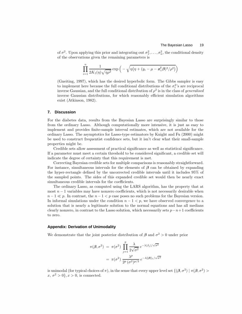
The Bayesian Lasso 19
of σ2. Upon applying this prior and integrating out σ21 , . . . , σ
2n, the conditional density
of the observations given the remaining parameters is
n∏
i=1
1
2K1(η)√
ηρ2exp
(−
√η(η + (yi − µ − xT
i β)2/ρ2))
(Gneiting, 1997), which has the desired hyperbolic form. The Gibbs sampler is easyto implement here because the full conditional distributions of the σ2
i ’s are reciprocalinverse Gaussian, and the full conditional distribution of ρ2 is in the class of generalised
inverse Gaussian distributions, for which reasonably efficient simulation algorithmsexist (Atkinson, 1982).
7. Discussion
For the diabetes data, results from the Bayesian Lasso are surprisingly similar to thosefrom the ordinary Lasso. Although computationally more intensive, it is just as easy toimplement and provides finite-sample interval estimates, which are not available for theordinary Lasso. The asymptotics for Lasso-type estimators by Knight and Fu (2000) mightbe used to construct frequentist confidence sets, but it isn’t clear what their small-sampleproperties might be.
Credible sets allow assessment of practical significance as well as statistical significance.If a parameter must meet a certain threshold to be considered significant, a credible set willindicate the degree of certainty that this requirement is met.
Correcting Bayesian credible sets for multiple comparisons is reasonably straightforward.For instance, simultaneous intervals for the elements of β can be obtained by expandingthe hyper-rectangle defined by the uncorrected credible intervals until it includes 95% ofthe sampled points. The sides of this expanded credible set would then be nearly exactsimultaneous credible intervals for the coefficients.
The ordinary Lasso, as computed using the LARS algorithm, has the property that atmost n− 1 variables may have nonzero coefficients, which is not necessarily desirable whenn− 1 � p. In contrast, the n− 1 < p case poses no such problems for the Bayesian version.In informal simulations under the condition n − 1 < p, we have observed convergence to asolution that is nearly a legitimate solution to the normal equations and has all mediansclearly nonzero, in contrast to the Lasso solution, which necessarily sets p−n+1 coefficientsto zero.
Appendix: Derivation of Unimodality
We demonstrate that the joint posterior distribution of β and σ2 > 0 under prior
π(β, σ2) = π(σ2)
p∏
j=1
λ
2√
σ2e−λ|βj |/
√σ2
= π(σ2)λp
2p (σ2)p/2e−λ‖β‖1/
√σ2
is unimodal (for typical choices of π), in the sense that every upper level set {(β, σ2) | π(β, σ2) >x, σ2 > 0}, x > 0, is connected.

20 T. Park and G. Casella
Unimodality in this sense is immediate for densities that are log concave. Unfortunately,this isn’t quite true in this case, but we can instead show that it is true under a continuoustransformation with continuous inverse, which will prove unimodality just as effectively,since connected sets are the images of connected sets under such a transformation.
The log posterior is
log(π(σ2)
)− n + p − 1
2log(σ2) − 1
2σ2‖y − Xβ‖2
2 − λ‖β‖1/√
σ2 (9)
after dropping all additive terms that involve neither β nor σ2. Consider the transformationdefined by
φ ↔ β/√
σ2 ρ ↔ 1/√
σ2,
which is continuous with a continuous inverse when 0 < σ2 < ∞. Note that this is simplyintended as a coordinate transformation, not as a transformation of measure (i.e. no Jaco-bian), so that upper level sets for the new parameters correspond under the transformationto upper level sets for the original parameters. In the transformed parameters, (9) becomes
log(π(1/ρ2
))+ (n + p − 1) log(ρ) − 1
2‖ρy − Xφ‖2
2 − λ‖φ‖1, (10)
where π is the prior density for σ2. The second and fourth terms are clearly concavein (ρ, φ), and the third term is a concave quadratic in (ρ, φ). Thus, the expression isconcave if log
(π(1/ρ2)
)is concave (because a sum of concave functions is concave). Func-
tion log(π(1/ρ2)
)is concave if, for instance, the prior on σ2 is the inverse gamma prior (5)
or the scale-invariant prior 1/σ2.The log posterior is thus unimodal in the sense that every upper level set is connected,
though this does not guarantee a unique maximiser. A sufficient condition for a uniquemaximiser is that the X matrix has full rank and y is not in the column space of X, sincethis makes the third term of (10) strictly concave.
References
Andrews, D. F., and Mallows, C. L. (1974), “Scale Mixtures of Normal Distributions,”Journal of the Royal Statistical Society, Ser. B, 36, 99–102.
Athreya, K. B. (1986), “Another Conjugate Family for the Normal Distribution,” Statistics
& Probability Letters, 4, 61–64.
Atkinson, A. C. (1982), “The Simulation of Generalized Inverse Gaussian and HyperbolicRandom Variables,” SIAM Journal on Scientific and Statistical Computing, 3, 502–515.
Booth, J. G., and Hobert, J. P. (1999), “Maximizing Generalized Linear Mixed Model Like-lihoods with an Automated Monte Carlo EM Algorithm,” Journal of the Royal Statistical
Society, Ser. B, 61, 265–285.
Box, G. E. P., and Tiao, G. C. (1973), Bayesian Inference in Statistical Analysis, Addison-Wesley.
Casella, G. (2001), “Empirical Bayes Gibbs Sampling,” Biostatistics, 2, 485–500.

The Bayesian Lasso 21
Chhikara, R. S., and Folks, L. (1989), The Inverse Gaussian Distribution: Theory, Method-
ology, and Applications, Marcel Dekker Inc.
Clyde, M., and George, E. I. (2000), “Flexible Empirical Bayes Estimation for Wavelets,”Journal of the Royal Statistical Society, Ser. B, 62, 681–698.
Clyde, M., Parmigiani, G., and Vidakovic, B. (1998), “Multiple Shrinkage and SubsetSelection in Wavelets,” Biometrika, 85, 391–401.
Efron, B., Hastie, T., Johnstone, I., and Tibshirani, R. (2004), “Least Angle Regression,”The Annals of Statistics, 32, 407–499.
Figueiredo, M. A. T. (2003), “Adaptive Sparseness for Supervised Learning,” IEEE Trans-
actions on Pattern Analysis and Machine Intelligence, 25, 1150–1159.
Frank, I. E., and Friedman, J. H. (1993), “A Statistical View of Some Chemometrics Re-gression Tools (Disc: P136-148),” Technometrics, 35, 109–135.
Fu, W. J. (1998), “Penalized Regressions: The Bridge versus the Lasso,” Journal of Com-
putational and Graphical Statistics, 7, 397–416.
George, E. I., and McCulloch, R. E. (1993), “Variable selection via Gibbs sampling,” Journal
of the American Statistical Association, 88, 881–889.
— (1997), “Approaches for Bayesian Variable Selection,” Statistica Sinica, 7, 339–374.
Gneiting, T. (1997), “Normal Scale Mixtures and Dual Probability Densities,” Journal of
Statistical Computation and Simulation, 59, 375–384.
Hastie, T., Tibshirani, R., and Friedman, J. H. (2001), The Elements of Statistical Learning:
Data Mining, Inference, and Prediction, Springer-Verlag Inc.
Ishwaran, H., and Rao, J. S. (2005), “Spike and Slab Variable Selection: Frequentist andBayesian Strategies,” Annals of Statistics, 33, 730–773.
Jørgensen, B. (1987), “Exponential Dispersion Models,” Journal of the Royal Statistical
Society, Ser. B, 49, 127–162.
Knight, K., and Fu, W. (2000), “Asymptotics for Lasso-Type Estimators,” The Annals of
Statistics, 28, 1356–1378.
McCulloch, C. E. (1997), “Maximum Likelihood Algorithms for Generalized Linear MixedModels,” Journal of the American Statistical Association, 92, 162–170.
Mitchell, T. J., and Beauchamp, J. J. (1988), “Bayesian Variable Selection in Linear Regres-sion (C/R: p1033-1036),” Journal of the American Statistical Association, 83, 1023–1032.
Osborne, M. R., Presnell, B., and Turlach, B. A. (2000), “A New Approach to VariableSelection in Least Squares Problems,” IMA Journal of Numerical Analysis, 20, 389–404.
Rosset, S., and Zhu, J. (2004), “Discussion of “Least Angle Regression” By Efron et. al.”Annals of Statistics, 32, 469–475.
Smyth, G. (2005), statmod: Statistical Modeling ; R package version 1.1.1.
22 T. Park and G. Casella
Tibshirani, R. (1996), “Regression Shrinkage and Selection Via the Lasso,” Journal of the
Royal Statistical Society, Ser. B, 58, 267–288.
West, M. (1984), “Outlier Models and Prior Distributions in Bayesian Linear Regression,”Journal of the Royal Statistical Society, Ser. B, 46, 431–439.
— (1987), “On Scale Mixtures of Normal Distributions,” Biometrika, 74, 646–648.
Yuan, M., and Lin, Y. (2005), “Efficient Empirical Bayes Variable Selection and Esimationin Linear Models,” Journal of the American Statistical Association, 100, 1215–1225.