the behavior of stock-market prices eugene f. fama the...
TRANSCRIPT

The Behavior of Stock-Market Prices
Eugene F. Fama
The Journal of Business, Vol. 38, No. 1. (Jan., 1965), pp. 34-105.
Stable URL:
http://links.jstor.org/sici?sici=0021-9398%28196501%2938%3A1%3C34%3ATBOSP%3E2.0.CO%3B2-6
The Journal of Business is currently published by The University of Chicago Press.
Your use of the JSTOR archive indicates your acceptance of JSTOR's Terms and Conditions of Use, available athttp://www.jstor.org/about/terms.html. JSTOR's Terms and Conditions of Use provides, in part, that unless you have obtainedprior permission, you may not download an entire issue of a journal or multiple copies of articles, and you may use content inthe JSTOR archive only for your personal, non-commercial use.
Please contact the publisher regarding any further use of this work. Publisher contact information may be obtained athttp://www.jstor.org/journals/ucpress.html.
Each copy of any part of a JSTOR transmission must contain the same copyright notice that appears on the screen or printedpage of such transmission.
The JSTOR Archive is a trusted digital repository providing for long-term preservation and access to leading academicjournals and scholarly literature from around the world. The Archive is supported by libraries, scholarly societies, publishers,and foundations. It is an initiative of JSTOR, a not-for-profit organization with a mission to help the scholarly community takeadvantage of advances in technology. For more information regarding JSTOR, please contact [email protected].
http://www.jstor.orgMon Mar 3 11:30:17 2008
THE BEHAVIOR OF STOCK-MARKET PRICES*
EUGENE F. FAMA?
FOR many years the following ques- tion has been a source of continuing controversy in both academic and
business circles: To what extent can the past history of a common stock's price be used to make meaningful predictions concerning the future price of the stock? Answers to this question have been pro- vided on the one hand by the various chartist theories and on the other hand by the theory of random walks.
Although there are many different chartist theories, they all make the same basic assumption. That is, they all as- sume that the past behavior of a securi- ty's price is rich in information concern- ing its future behavior. History repeats itself in that "patterns" of past price be-
*This study has profited from the criticisms, suggestions, and technical assistance of many dif- ferent people. In particular I wish to express my gratitude to Professors William Alberts, Lawrence Fisher, Robert Graves, James Lorie, Merton Miller, Harry Roberts, and Lester Telser, all of the Gradu- ate School of Business, University of Chicago. I wish es~ecially to thank Professors Miller and Roberts for providing not only continuous intellectual stimula- tion but also painstaking care in reading the various preliminary drafts.
Many of the ideas in this paper arose out of the work of Benoit Mandelbrot o i the IBM Watson Re- search Center. I have profited not only from the written work of Dr. Mandelbrot but also from many invaluable discussion sessions.
Work on this paper was supported in part by funds from a grant by the Ford Foundation to the Graduate School of Business of the University of Chicago, and in part by funds granted to the Center for Research in Security Prices of the School by the National Science Foundation. Extensive computer time was provided by the 7094 Computation Center of the University of Chicago.
'f Assistant professor of fmance, Graduate School of Business, University of Chicago.
34
havior will tend to recur in the future. Thus, if through careful analysis of price charts one develops an understanding of these "patterns," this can be used to predict the future behavior of prices and in this way increase expected gains.l
By contrast the theory of random walks says that the future path of the price level of a security is no more pre- dictable than the path of a series of cumulated random numbers. In statisti- cal terms the theory says that successive price changes are independent, identical- ly distributed random variables. Most simply this implies that the series of price changes has no memory, that is, the past cannot be used to predict the future in any meaningful way.
The purpose of this paper will be to discuss first in more detail the theorv underlying the random-walk model and then to test the model's empirical validi- ty. The main conclusion will be that the data seem to present consistent and
for the This im-plies, of course, that chart reading,- . -. though per-aps an interesting pastime, is of no real value to the stock market in- vestor. This is an extreme statement and the reader is certainly free to take exception' We suggest, however, that since the empirical evidence produced by this and other studies in support of the
random-wa1k is volumi-nous, the counterarguments of the chart
will be completely lacking in force if they are ed by empirical work.
The Dow Theory, of course, is the best known example of a chartist theory.

35 BEHAVIOR OF STOCK-MARKET PRICES
11. THEORY WALKSOF RANDOM IN STOCKPRICES
The theory of random walks in stock prices actually involves two separate hypotheses: (1) successive price changes are independent, and (2) the changes conform to some probability distribution. weshall now examine each of these hypotheses in detail.
A. INDEPENDENCE
I. MEANING OF INDEPENDENCE
In statistical terms independence means that the probability distribution for the price change during time period t is inde- pendent of the sequence of price changes during previous time periods. That is, knowledge of the sequence of price changes leading up to time period t is of no help in assessing the probability distribution for the price change during time period t.2
Now in fact we can probably never hope to find a time series that is charac- teriled by perfect independence. Thus, strictly speaking, the random walk the- ory cannot be a completely accurate de- scription of reality. For practical pur- poses, however, we may be willing to accept the independence assumption of the model as long as the dependence in the series of successive price changes is not above some "minimum acceptable" level.
what a ((minimumaccept-
able" level of dependence depends, of course, on the particular problem that
More precisely, independence means that
Pr(xt = xl xtFl, xtF2, . . .) = Pr(xt= X). ,. where the term on the right of the equality sign is the unconditional probability that the price change during time t will take the value X , whereas the term on the left is the conditional probability that the price change will take the value x , conditional on the knowledge that previous price changes took the values xt-1, x t - ~ ,etc.
one is trying to solve. For example, some- one who is doing statistical work in the stock market may wish to decide whether dependence in the series of successive price changes is sufficient to account for Some particular property of the distribu-tion of price changes. If the actual de- pendence in the series is not sufficient to account for the property in question, the statistician may be justified in accepting the independence hypothesis as an ade- quate description of reality.
By contrast the stock market trader has a much more practical criterion for judging what constitutes important de- pendence in successive price changes. For his purposes the random walk model is valid as long as knowledge of the past behavior of the series of price changes cannot be used to increase expected gains. More specifically, the independence as-sumption is an adequate description of reality as long as the actual degree of dependence in the series of price changes is sufficient to the past of the series to be used to predict the future in a way which makes expected profits greater than they would be under a ""Ive buy-and-hold
Dependence that is important from the trader's point of view need not be im- portant from a statistical point of view, and conversely dependence which is im- portant for statistical purposes need not be important for investment purposes.
examplel we know that On
nate the price a increases by E and then decreases by E .
From a statistical point of view knowl- edge of this dependence would be impor- tant information since it tells us quite a bit about the shape of the distribution of price changes. For trading purposes, however, as long as E is very small, this perfect, negative, is unimportant. Any profits the trader

36 THE JOURNAL OF BUSINESS
may hope to make from it would be washed away in transactions costs.
In Section V of this paper we shall be concerned with testing independence from the point of view of both the statis- tician and the trader. At this point, how- ever, the next logical step in the develop- ment of a theory of random walks in stock prices is to consider market situa- tions and mechanisms that are consistent with independence in successive price changes. The procedure will be to con- sider first the simplest situations and then to successively introduce complica- tions.
2. MARKET SITUATIONS CONSISTENT
WITH INDEPENDENCE .
Independence '' successive .price
with the random-walk hypothesis. In order to justify this statement, however, it will be necessary now to discuss more fully the process of price determination in an intrinsic-value-random-walk mar-ket.
Assume that at any point in time there exists, a t least implicitly, an intrin- sic value for each security. The intrinsic value of a given security depends on the earnings prospects of the company which in turn are related to economic and po- litical factors some of which are peculiar to this company and some of which affect other companies as well.3
We stress, however, that actual mar- ket prices need not correspond to intrin- sic values. In a world of uncertainty in- trinsic values are not known exactly.
changes for a given may s l m ~ l ~Thus there can always be disagreement reflect a price mechanism which is totally unrelated to real-world economic and po- litical events. That stock prices be just the accumulation of many bits of randomly generated noise> where by noise in this case we mean psychological and other factors peculiar to different individuals which determine the types of "bets" they are willing to place On
different companies. Even random walk theorists>
would find such a view of the market un-appealing. some people may be primarily lnotivated there are many individuals and institutions that seem to base their actions in the market on an painstaking) of economic and political circumstances. That is, there are many private investors and institutions who believe that individual securities have "intrinsic values" which depend on eco- nOmicand politica1 that affect in-dividual companies.
~h~ existence of intrinsic values for individual securities is not inconsistent
among individuals, and in this way ac-tual prices and intrinsic values can differ. Henceforth uncertainty or disagreement concerning intrinsic values will come under the general heading of "noise" in the market.
Inaddition, intrinsic values can them-selves change across time as a result of either new infomation or trend. New in- formation may concern such things as the success of a current research and de- velopment project, a change in manage- ment, a tariff imposed on the industry's product by a foreign country, an increase in industrial production or any other actual or anticipated change in a factor which is likely to affectthe company's prospects.
3 We can think of intrinsic values in either of two ways. First, perhaps they just represent market conventions for evaluating the worth of a securitv -by relating i t to various factors which affect the earnings of a company. On the other hand, intrinsic values may actually represent equilibrium prices in the economist's sense, i.e., prices that evolve from some dynamic general equilibrium model. For our purposes i t is irrelevant which point of view one takes.

BEHAVIOR OF STOCK-MARKET PRICES 37
On the other hand, an anticipated long-term trend in the intrinsic value of a given security can arise in the following way.4 Suppose we have two unlevered companies which are identical in all re- spects except dividend policy. That is, both companies have the same current and anticipated investment opportuni- ties, but they finance these opportunities in different ways. In particular, one com- pany pays out all of its current earnings as dividends and finances new invest-ment by issuing new common shares. The other company, however, finances new investment out of current earnings and pays dividends only when there is money left over. Since shares in the two companies are subject to the same degree of risk, we would expect their expected rates of returns to be the same. This will be the case, however, only if the shares of the company with the lower dividend payout have a higher expected rate of price increase than do the shares of the high-payout company. In this case the trend in the price level is just part of the expected return to equity. Such a trend is not inconsistent with the random-walk hyp~thes is .~
The simplest rationale for the inde- pendence assumption of the random walk model was proposed first, in a rather vague fashion, by Bachelier [6] and then much later but more explicitly by Os- borne [42].The argument runs as follows: If successive bits of new information arise independently across time, and if noise or uncertainty concerning intrinsic values does not tend to follow any con- sistent pattern, then successive price changes in a common stock will be inde- pendent.
As with many other simple models,
A trend in the price level, of course, corresponds to a non-zero mean in the distribution of price changes.
however, the assumptions upon which the Bachelier-Osborne model is built are rather extreme. There is no strong reason to expect that each individual's estimates of intrinsic values will be independent of the estimates made by others (i.e., noise may be generated in a dependent fashion). For example, certain individ- uals or institutions may be opinion lead- ers in the market. That is, their actions may induce people to change their opin- ions concerning the prospects of a given company. In addition there is no strong reason to expect successive bits of new information to be generated independ- ently across time. For example, good news may tend to be followed more often by good news than by bad news, and bad news may tend to be followed more often by bad news than by good news. Thus there may be dependence in either the noise generating process or in the process generating new information, and these may in turn lead to dependence in suc- cessive price changes.
Even in a situation where there are dependencies in either the information or the noise generating process, however, it is still possible that there are offsetting mechanisms in the market which tend to produce independence in price changes for individual common stocks. For ex-ample, let us assume that there are many sophisticated traders in the stock market and that sophistication can take two forms: (1) some traders may be much better a t predicting the appearance of new information and estimating its ef- fects on intrinsic values than others, while (2) some may be much better at doing statistical analyses of price be-havior. Thus these two types of sophis- ticated traders can be roughly thought of as superior intrinsic-value analysts
A lengthy and rigorous justification for these statements is given by Miller and Modigliani [40].

38 THE JOURNAL OF BUSINESS
and superior chart readers. We further assume that, although there are some- times discrepancies between actual prices and intrinsic values, sophisticated trad- ers in general feel that actual prices usu- ally tend to move toward intrinsic val- ues.
Suppose now that the noise generating process in the stock market is dependent. More specifically assume that when one person comes into the market who thinks the current price of a security is above or below its intrinsic value, he tends to attract other people of like feelings and he causes some others to change their opinions unjustifiably. In itself this type of dependence in the noise generat- ing process would tend to produce "bub- bles" in the price series, that is, periods of time during which the accumulation of the same type of noise causes the price level to run well above or below the in- trinsic value.
If there are many sophisticated traders in the market, however, they may cause these "bubbles" to burst before they have a chance to really get under way. For example, if there are many sophisti- cated traders who are extremely good a t estimating intrinsic values, they will be able to recognize situations where the price of a common stock is beginning to run up above its intrinsic value. Since they expect the price to move eventually back toward its intrinsic value, they have an incentive to sell this security or to sell it short. If there are enough of these sophisticated traders, they may tend to prevent these "bubbles" from ever oc- curring. Thus their actions will neutral- ize the dependence in the noise-generat- ing process, and successive price changes will be independent.
In fact, of course, in a world of uncer- tainty even sophisticated traders cannot always estimate intrinsic values exactly.
The effectiveness of their activities in erasing dependencies in the series of price changes can, however, be reinforced by another neutralizing mechanism. As long as there are important dependencies in the series of successive price changes, op- portunities for trading profits are avail- able to any astute chartist. For example, once they understand the nature of the dependencies in the series of successive price changes, sophisticated chartists will be able to identify statistically situations where the price is beginning to run up above the intrinsic value. Since they ex- pect that the price will eventually move back toward its intrinsic value, they will sell. Even though they are vague about intrinsic values, as long as they have sufficient resources their actions will tend to erase dependencies and to make actual prices closer to intrinsic values.
Over time the intrinsic value of a common stock will change as a result of new information, that is, actual or an- ticipated changes in any variable that affects the prospects of the company. If there are dependencies in the process generating new information, this in it- self will tend to create dependence in successive price changes of the security. If there are many sophisticated traders in the market, however, they should eventually learn that it is profitable for them to attempt to interpret both the price effects of current new information and of the future information implied by the dependence in the information gen- erating process. In this way the actions of these traders will tend to make price changes inde~endent .~
Moreover, successive price changes may be independent even if there is usu- ally consistent vagueness or uncertainty
In essence dependence in the information gen- erating process is itself relevant information which the astute trader should consider.
39 BEHAVIOR OF STOCK-MARKET PRICES
surrounding new information. For exam- ple, if uncertainty concerning the im- portance of new information consistently causes the market to underestimate the effects of new information on intrinsic values, astute traders should eventually learn that it is profitable to take this into account when new information appears in the future. That is, by examining the history of prices subsequent to the influx of new information it will become clear that profits can be made simply by buy- ing (or selling short if the information is pessimistic) after new information comes into the market since on the average ac- tual prices do not initially move all the way to their new intrinsic values. If many traders attempt to capitalize on this opportunity, their activities will tend to erase any consistent lags in the adjustment of actual prices to changes in intrinsic values.
The above discussion implies, of course, that, if there are many astute traders in the market, on the average the full effects of new information on in- trinsic values will be reflected nearly in- stantaneously in actual prices. In fact, however, because there is vagueness or uncertainty surrounding new informa-tion, "instantaneous adjustment" really has two implications. First, actual prices will initially overadjust to the new in- trinsic values as often as they will under- adjust. Second, the lag in the complete adjustment of actual prices to successive new intrinsic values will itself be an in- dependent random variable, sometimes preceding the new information which is the basis of the change (i.e., when the information is anticipated by the market before it actually appears) and some-times following. It is clear that in this case successive price changes in individ- ual securities will be independent random variables,
I n sum, this discussion is sufficient to show that the stock market may conform to the independence assumption of the random walk model even though the processes generating noise and new in- formation are themselves dependent. We turn now to a brief discussion of some of the implications of independence.
3. IMPLICATIONS OF INDEPENDENCE
In the previous section we saw that one of the forces which helps to produce independence of successive price changes may be the existence of sophisticated traders, where sophistication may mean either (1) that the trader has a special talent in detecting dependencies in series of prices changes for individual securi- ties, or (2) that the trader has a special talent for predicting the appearance of new information and evaluating its ef- fects on intrinsic values. The first kind of trader corresponds to a superior chart reader, while the second corresponds to a superior intrinsic value analyst.
Now although the activities of the chart reader may help to produce inde- pendence of successive price changes, once independence is established chart reading is no longer a profitable activity. Jn a series of independent price changes, the past history of the series cannot be used to increase expected profits.
Such dogmatic statements cannot be applied to superior intrinsic-value analy- sis, however. In a dynamic economy there will always be new information which causes intrinsic values to change over time. As a result, people who can consistently predict the appearance of new information and evaluate its effects on intrinsic values will usually make larger profits than can people who do not have this talent. The fact that the activ- ities of these superior analysts help to make successive price changes independ-

40 THE JOURNAL OF BUSINESS
ent does not imply that their expected profits cannot be greater than those of the investor who follows some na'ive buy- and-hold policy.
It must be emphasized, however, that the comparative advantage of the supe- rior analyst over his less talented com- petitors lies in his ability to predict consistently the appearance of new in-formation and evaluate its impact on intrinsic values. If there are enough su- perior analysts, their existence will be sufficient to insure that actual market prices are, on the basis of all available information, best estimates of intrinsic values. In this way, of course, the supe- rior analysts make intrinsic value analy- sis a useless tool for both the average analyst and the average investor.
This discussion gives rise to three obvious question: (1) How many superior analysts are necessary to insure inde- pendence? (2) Who are the "superior" analysts? and (3) What is a rational in- vestment policy for an average investor faced with a random-walk stock market?
It is impossible to give a firm answer to the first question, since the effective- ness of the superior analysts probably depends more on the extent of their re- sources than on their number. Perhaps a single, well-informed and well-endowed specialist in each security is sufficient.
It is, of course, also very difficult to identify ex ante those people that qualify as superior analysts. Ex post, however, there is a simple criterion. A superior analyst is one whose gains over many periods of time are consistently greater than those of the market. Consistently is the crucial word here, since for any given short period of time, even if there are no superior analysts, in a world of random walks some people will do much better than the market and some will do much worse.
Unfortunately, by this criterion this author does not qualify as a superior analyst. There is some consolation, how- ever, since, as we shall see later, other more market-tested institutions do not seem to qualify either.
Finally, let us now briefly formulate a rational investment policy for the aver- age investor in a situation where stock prices follow random walks and a t every point in time actual prices represent good estimates of intrinsic values. In such a situation the primary concern of the average investor should be portfolio anal- ysis. This is really three separate prob- lems. First, the investor must decide what sort of tradeoff between risk and expected return he is willing to accept. Then he must attempt to classify securi- ties according to riskiness, and finally he must also determine how securities from different risk classes combine to form portfolios with various combinations of risk and return.?
In essence in a random-walk market the security analysis problem of the aver- age investor is greatly simplified. If actu-al prices a t any point in time are good estimates of intrinsic values, he need not be concerned with whether individual securities are over- or under-priced. If he decides that his portfolio requires an additional security from a given risk class, he can choose that security ran- domly from within the class. On the aver- age any security so chosen will have about the same effect on the expected re- turn and riskiness of his portfolio.
B. T H E DISTRIBUTION OF PRICE CHANGES
1. INTRODUCTION
The theory of random walks in stock prices is based on two hypotheses: (1) successive price changes in an indi-
7 For a more complete formulation of the port- folio analysis problem see Markowitz [39].

BEHAVIOR OF STOCK-MARKET PRICES 41
vidual security are independent, and (2) the price changes conform to some probability distribution. Of the two hy- potheses independence is the most impor- tant. Either successive price changes are independent (or at least for all practical purposes independent) or they are not; and if they are not, the theory is not valid. All the hypothesis concerning the distribution says, however, is that the price changes conform to some probabili-ty distribution. In the general theory of random walks the form or shape of the distribution need not be specified. Thus any distribution is consistent with the theory as long as it correctly character- izes the process generating the price change^.^
From the point of view of the investor, however, specification of the shape of the distribution of price changes is extremely helpful. In general, the form of the dis- tribution is a major factor in determining the riskiness of investment in common stocks. For example, although two differ- ent possible distributions for the price changes may have the same mean or ex- pected price change, the probability of very large changes may be much greater for one than for the other.
The form of the distribution of price changes is also important from an aca- demic point of view since it provides de- scriptive information concerning the na- ture of the process generating price changes. For example, if very large price
O f course, the theory does imply that the pa- rameters o f the distribution should be stationary or fixed. As long as independence holds, however, sta- tionarity can be interpreted loosely. For example, i f independence holds i n a strict fashion, then for the purposes o f the investor the random walk model is a valid approximation t o reality even though the parameters o f the probability distribution o f the price changes m a y be non-stationary.
For statistical purposes stationarity implies simply that the parameters o f the distribution should be fixed a t least for the time period covered b y the data.
changes occur quite frequently, it may be safe to infer that the economic struc- ture that is the source of the price changes is itself subject to frequent and sudden shifts over time. That is, if the distribu- tion of price changes has a high degree of dispersion, it is probably safe to infer that, to a large extent, this is due to the variability in the process generating new information.
Finally, the form of the distribution of price changes is important information to anyone who wishes to do empirical work in this area. The power of a statis- tical tool is usually closely related to the type of data to which it is applied. In fact we shall see in subsequent sections that for some probability distributions important concepts like the mean and variance are not meaningful.
2. THE BACHELIER-OSBORNE MODEL
The first complete development of a theory of random walks in security prices is due to Bachelier [6], whose original work first appeared around the turn of the century. Unfortunately his work did not receive much attention from econo- mists, and in fact his model was inde- pendently derived by Osborne [42] over fifty years later. The Bachelier-Osborne model begins by assuming that price changes from transaction to transaction in an individual security are independ- ent, identically distributed random vari- ables. It further assumes that transac- tions are fairly uniformly spread across time, and that the distribution of price changes from transaction to transaction has finite variance. If the number of transactions per day, week, or month is very large, then price changes across these differencing intervals will be sums of many independent variables. Under these conditions the central-limit theo- rem leads us to expect that the daily,

42 THE JOURNAL OF BUSINESS
weekly, and monthly price changes will each have normal or Gaussian distribu- tions. Moreover, the variances of the dis- tributions will be proportional to the re- spective time intervals. For example, if u2 is the variance of the distribution of the daily changes, then the variance for the distribution of the weekly changes should be approximately 5a2.
Although Osborne attempted to give an empirical justification for his theory, most of his data were cross-sectional and could not provide an adequate test. Moore and Kendall, however, have pro- vided empirical evidence in support of the Gaussian hypothesis. Moore [41, pp. 116-231 graphed the weekly first differ- ences of log price of eight NYSE common stocks on normal probability paper. Al- though the extreme sections of his graphs seem to have too many large price changes, Moore still felt the evidence was strong enough to support the hy- pothesis of approximate normality.
Similarly Kendall [26] observed that weekly price changes in British common stocks seem to be approximately nor-mally distributed. Like Moore, however, he finds that most of the distributions of price changes are leptokurtic; that is, there are too many values near the mean and too many out in the extreme tails. In one of his series some of the extreme observations were so large that he felt compelled to drop them from his subse- quent statistical tests.
3. U N D E L B R O T AND THE GENERALIZED
CENTRAL-LIMIT THEOREM
The Gaussian hypothesis was not seri- ously questioned until recently when the work of Benoit Mandelbrot first began to appear.g Mandelbrot's main assertion is
His main work in this area is [37]. References to his other works are found through this report and in the bibliography,
that, in the past, academic research has too readily neglected the implications of the leptokurtosis usually observed in empirical distributions of price changes.
The presence, in general, of leptokur- tosis in the empirical distributions seems indisputable. In addition to the results of Kendall [26] and Moore [41] cited above, Alexander [I] has noted that Os- borne's cross-sectional data do not really support the normality hypothesis; there are too many changes greater than + 10 per cent. Cootner [lo] has developed a whole theory in order to explain the long tails of the empirical distributions. Final- ly, Mandelbrot [37, Fig. 11 cites other examples to document empirical lepto- kurtosis.
The classic approach to this problem has been to assume that the extreme values are generated by a different mech- anism than the majority of the observa- tions. Consequently one tries a posteriori to find '(causal" explanations for the large observations and thus to rational- ize their exclusion from any tests carried out on the body of the data.1° Unlike the statistician, however, the investor cannot ignore the possibility of large price changes before committing his funds, and once he has made his decision to invest, he must consider their effects on his wealth.
Mandelbrot feels that if the outliers are numerous, excluding them takes away much of the significance from any tests carried out on the remainder of the data. This exclusion process is all the more subject to criticism since probabil- ity distributions are available which ac- curately represent the large observations
When extreme values are excluded from the sample, the procedure is often called "trimming." Another technique which involves reducing the size of extreme observations rather than excluding them is called "Winsorization." For a discussion see J, W. Tukey [45].

43 BEHAVIOR OF STOC 'R-MARKET PRICES
as well as the main body of the data. The distributions referred to are mem- bers of a special class which Mandelbrot has labeled stable Paretian. The mathe- matical properties of these distributions are discussed in detail in the appendix to this paper. At this point we shall merely introduce some of their more important descriptive properties.
Parameters of stable Paretian distri-butions.-Stable Paretian distributions have four parameters: (1) a location pa- rameter which we shall call 6, (2) a scale parameter henceforth called y, (3) an index of skewness, 6, and (4) a measure of the height of the extreme tail areas of the distribution which we shall call the characteristic exponent a.ll
When the characteristic exponent a is greater than 1, the location parameter 6 is the expectation or mean of the distri- bution. The scale parameter y can be any positive real number, but 6, the index of skewness, can only take values in the in- terval -1 < 6 < 1. When6 = Othedis-tribution is symmetric. When > 0 the distribution is skewed right (i.e., has a long tail to the right), and the degree of right skewness is larger the larger the value of 6. Similarly, when < 0 the dis- tribution is skewed left, and the degree of left skewness is larger the smaller the value of 6.
The characteristic exponent a of a stable Paretian distribution determines the height of, or total probability con- tained in, the extreme tails of the distri- bution, and can take any value in the interval 0 < a 5 2. When a = 2, the rel- evant stable Paretian distribution is the
l1The derivation of most of the important prop- erties of stable Paretian distributions is due to P. Levy [29]. A rigorous and compact mathematical treatment of the theory can be found in B. V. Gnedenko and A. N. Kolmogorov [17]. A more comprehensive mathematical treatment can be found in Mandelbrot [37].
normal or Gaussian distribution. When a is in the interval 0 < a < 2, the extreme tails of the stable Paretian distributions are higher than those of the normal dis- tribution, and the total probability in the extreme tails is larger the smaller the value of a. The most important conse- quence of this is that the variance exists (i.e., is finite) only in the extreme case a = 2. The mean, however, exists as long as a > 1.12
Mandelbrot's hypothesis states that for distributions of price changes in spec- ulative series, a is in the interval 1 < a < 2, so that the distributions have means but their variances are infinite. The Gaussian hypothesis, on the other hand, states that a is exactly equal to 2. Thus both hypotheses assume that the distri- bution is stable Paretian. The disagree- ment between them concerns the value of the characteristic exponent a.
Properties of stable Paretian distribu- tions.-Two important properties of sta- ble Paretian distributions are (1) stabil- ity or invariance under addition, and (2) the fact that these distributions are the only possible limiting distributions for sums of independent, identically distrib- uted, random variables.
By definition, a stable Paretian distri- bution is any distribution that is stable or invariant under addition. That is, the distribution of sums of independent, identically distributed, stable Paretian variables is itself stable Paretian and, except for origin and scale, has the same form as the distribution of the individual summands. Most simply, stability means that the values of the parameters a and /3 remain constant under addition.13
The property of stability is responsible
l2 For a proof of these statements see Gnedenko and Kolmogorov [17], pp. 179-83.
l3A more rigorous definition of stability is given in the appendix,

44 THE JOURNAL OF BUSINESS
for much of the appeal of stable Paretian distributions as descriptions of empirical distributions of price changes. The price change of a stock for any time interval can be regarded as the sum of the changes from transaction to transaction during the interval. If transactions are fairly uniformly spread over time and if the changes between transactions are inde- pendent, identically distributed, stable Paretian variables, then daily, weekly, and monthly changes will follow stable Paretian distributions of exactly the same form, except for origin and scale. For example, if the distribution of daily changes is stable Paretian with location parameter 6 and scale paremeter y, the distribution of weekly (or five-day) changes will also be stable Paretian with location parameter 56 and scale parame- ter 5y. I t would be very convenient if the form of the distribution of price changes were independent of the differ- encing interval for which the changes were computed.
I t can be shown that stability or in- variance under addition leads to a most important corollary property of stable Paretian distributions; they are the only possible limiting distributions for sums of independent, identically distributed, random variables.14 I t is well known that if such variables have finite variance, the limiting distribution for their sum will be the normal distribution. If the basic vari- ables have infinite variance, however, and if their sums follow a limiting dis- tribution, the limiting distribution must be stable Paretian with 0 < a < 2.
In light of this discussion we see that Mandelbrot's hypothesis can actually be viewed as a generalization of the central-limit theorem arguments of Bachelier and Osborne to the case where
l4 For a proof see Gnedenko and Kolmogorov [17], pp. 162-63.
the underlying distributions of price changes from transaction to transaction are allowed to have infinite variances. In this sense, then, Mandelbrot's version of the theory of random walks can be re- garded as a broadening rather than a contradiction of the earlier Bachelier-Osborne model.
Conclusion.-Mandelbrot's hypothesis that the distribution of price changes is stable Paretian with characteristic expo- nent a < 2 has far reaching implications. For example, if the variances of distribu- tions of price changes behave as if they are infinite, many common statistical tools which are based on the assumption of a finite variance either will not work or may give very misleading answers. Getting along without these familiar tools is not going to be easy, and before parting with them we must be sure that such a drastic step is really necessary. At the moment, the most impressive single piece of evidence is a direct test of the infinite variance hypothesis for the case of cotton prices. Mandelbrot 137, Fig. 2 and pp. 404-71 computed the sam- ple second moments of the first differ- ences of the logs of cotton prices for increasing sample sizes of from 1to 1,300 observations. He found that the sample moment does not settle down to any limiting value but rather continues to vary in absolutely erratic fashion, pre- cisely as would be expected under his hypothesis.15
As for the special but important case
l6 The second moment of a random variable x is just E(s2) .The variance is just the second moment minus the square of the mean. Since the mean is assumed to be a constant, tests of the sample second moment are also tests of the sample variance.
In an earlier privately circulated version of [37] Mandelbrot tested his hypothesis on various other series of speculative prices. Although the results in general tended to support his hypothesis, they were neither as extensive nor as conclusive as the tests on cotton prices.

45 BEHAVIOR OF STOCK-M ARKET PRICES
of common-stock prices, no published evidence for or against Mandelbrot's the- ory has yet been presented. One of our main goals here will be to attempt to test Mandelbrot's hypothesis for the case of stock prices.
C. THINGS TO COME
Except for the concluding section, the remainder of this paper will be concerned with reporting the results of extensive tests of the random walk model of stock price behavior. Sections I11 and IV will examine evidence on the shape of the distribution of price changes. Section I11 will be concerned with common statisti- cal tools such as frequency distributions and normal probability graphs, while Section IV will develop more direct tests of Mandelbrot's hypothesis that the characteristic exponent a for these dis- tributions is less than 2. Section V of the paper tests the independence assumption of the random-walk model. Finally, Sec- tion VI will contain a summary of pre- vious results, and a discussion of the im- plications of these results from various points of view.
111. A FIRSTLOOKAT THE EM-PIRICAL DISTRIBUTIONS
A. INTRODUCTION
In this section a few simple techniques will be used to examine distributions of daily stock-price changes for individual securities. If Mandelbrot's hypothesis that the distributions are stable Paretian with characteristic exponents less than 2 is correct, the most important feature of the distributions should be the length of their tails. That is, the extreme tail areas should contain more relative frequency than would be expected if the distribu- tions were normal. In this section no attempt will be made to decide whether
the actual departures from normality are sufficient to reject the Gaussian hypothe- sis. The only goal will be to see if the departures are usually in the direction predicted by the Mandelbrot hypothesis.
B. THE DATA
The data that will be used throughout this paper consist of daily prices for each of the thirty stocks of the Dow-Jones Industrial Average.16 The time periods vary from stock to stock but usually run from about the end of 1957 to September 26, 1962. The final date is the same for all stocks, but the initial date varies from January, 1956 to April, 1958. Thus there are thirty samples with about 1,200-1,700 observations per sample.
The actual tests are not performed on the daily prices themselves but on the first differences of their natural loga-rithms. The variable of interest is
where pt+l is the price of the security at the end of day t + 1, and p t is the price at the end of day t.
There are three main reasons for using changes in log price rather than simple price changes. First, the change in log price is the yield, with continuous com- pounding, from holding the security for that day." Second, Moore [41, pp. 13-15] has shown that the variability of simple price changes for a given stock is an in- creasing function of the price level of the stock. His work indicates that taking
l6 The data were very generously supplied by Professor Harry B. Ernst of Tufts University.
17 The proof of this statement goes as follows:
p t + l = pt exp (loge F)

46 TI-IE JOURNAL O F BUSINESS
logarithms seems to neutralize most of this price level effect. Third, for changes less than _f 15 per cent the change in log price is very close to the percentage price change, and for many purposes it is convenient to look at the data in terms of percentage price changes.18
In working with daily changes in log price, two special situations must be noted. They are stock splits and ex-divi- dend days. Stock splits are handled as follows: if a stock splits two for one on day t, its actual closing price on day t is doubled, and the difference between the logarithm of this doubled price and the logarithm of the closing price for day t - 1 is the first difference for day t. The first difference for day t + 1 is the differ- ence between the logarithm of the closing price on day t + 1 and the logarithm of the actual closing price on day t, the day of the split. These adjustments reflect the fact that the process of splitting a stock involves no change either in the asset value of the firm or in the wealth of the individual shareholder.
On ex-dividend days, however, other things equal, the value of an individual share should fall by about the amount of the dividend. To adjust for this the first difference between an ex-dividend day and the preceding day is computed as
where d is the dividend per share.Ig One final note concerning the data is
in order. The Dow-Jones Industrials are not a random sample of stocks from the New York Stock Exchange. The compo- nent companies are among the largest and most important in their fields. If the
l8Since, for our purposes, the variable of interest will always be the change in log price, the reader should note that henceforth when the words "price change" appear in the text, we are actually referring to the change in log price.
behavior of these blue-chips stocks differs consistently from that of other stocks in the market, the empirical results to be presented below will be strictly appli- cable only to the shares of large impor- tant companies.
One must admit, however, that the sample of stocks is conservative from the point of view of the Mandelbrot hypoth- esis, since blue chips are probably more stable than other securities. There is reason to expect that if such a sample conforms well to the Mandelbrot hypoth- esis, a random sample would fit even better.
C. FREQUENCY DISTRIBUTIONS
One very simple way of analyzing the distribution of changes in log price is to construct frequency distributions for the individual stocks. That is, for each stock the empirical proportions of price changes within given standard deviations of the mean change can be computed and com- pared with what would be expected if the distributions were exactly normal. This is done in Tables 1 and 2. In Table 1 the proportions of observations within 0.5, 1.0, 1.5, 2.0, 2.5, 3.0, 4.0, and 5.0 stand- ard deviations of the mean change, as well as the proportion greater than 5 standard deviations from the mean, are computed for each stock. In the first line of the body of the table the proportions for the unit normal distribution are given.
Table 2 gives a comparison of the unit normal and the empirical distributions.
l9 I recognize that because of tax effects and other considerations, the value of a share may not be ex- pected to fall by the full amount of the dividend. Because of uncertainty concerning what the correct adjustment should be, the price changes on ex-divi- dend days were discarded in an earlier version of the paper. Since the results reported in the earlier ver- sion differ very little from those to be presented below, i t seems that adding back the full amount of the dividend produces no important distortions in the empirical results.

47 BEHAVIOR OF STOCK-MARKET PRICES
Each entry in this table was computed umn (1) opposite Allied Chemical im-by taking the corresponding entry in plies that the empirical distribution con-Table 1and subtracting from it the entry tains about 7.6 per cent more of the for the unit normal distribution in Table total frequency within one-half standard 1. For example, the entry in column (1) deviation of the mean than would be Table 2 for Allied Chemical was found expected if the distribution were normal. by subtracting the entry in column (1) The number in column (9) implies that Table 1 for the unit normal, 0.3830, from in the empirical distribution about 0.16 the entry in column (1) Table 1 for per cent more of the total frequency is Allied Chemical, 0.4595. greater than five standard deviations
A positive number in Table 2 should from the mean than would be expected be interpreted as an excess of relative under the normal or Gaussian hypothe-frequency in the empirical distribution sis. over what would be expected for the Similarly, a negative number in the given interval if the distribution were table should be interpreted as a defi-normal. For example, the entry in col- ciency of relative frequency within the
TABLE 1
FREQUENCYDISTRIBUTIONS
Unit normal.. . . . . . . . . Allied Chemical.. . . . . . Alcoa . . . . . . . . . . . . . . . . American Can. . . . . . . . A.T.&T.. . . . . . . . . . . . . American Tobacco. . . . Anaconda. . . . . . . . . . . . Bethlehem Steel. . . . . . Chrysler . . . . . . . . . . . . . Du Pont . . . . . . . . . . . . . Eastman Kodak. . . . . . General Electric.- .--.--..--- . . . . . . . . . / .46311 ,74601 .87711 .9427/ ,97751 .9870/ 0.9970471 0.99940931 .0005907~ -
General Foods.. . . . . . . . . . . General Motors.. . . . . . . . . . Goodyear. . . . . . . . . . . . . . . . International Harvester.. . . International Nickel..International Nickel...~-- . . . . . ,4722,47221 .76351 .88331 .94131 ,96861 .98711 0.9951731 1.0000000~.8833 .9413 .9686 .9871 0.995173 1.0000000. . . . .I .7635 .0000000.0000000 International Paper.International . . . . . .Paper. . . . . . . .4444 ,7498 .8742 .9433 .9758 .9869 0.996545 1.0000000 .0000000 Johns Manville.Johns . . . . . . . . . .Manville. . . . . . . . . . . .4365 ,7377 .8730 ,9485 .9809 .9909 0.997510 0.9991701 ,0008299 Owens Illinois.Owens . . . . . . . . . . .Illinois. . . . . . . . . . . . .4778 .7389 .8909 .9466 .9717 .9838 0.997575 0.9991916 .0008084 Procter & Gamble. . . . . . . . ,5017 .7706 .8887 .9378 .9710 .9862 0.995853 0.9986178 .0013822 Sears. . . . . . . . . . . . . . . . . . . . ,5388 .7856 .9021 .9490 .9701 .9830 0.993528 0.9959547 ,0040453 Standard Oil iCa1if.l. . . . . . ,4584 .7348 .8724 .9439 ,9764 .9917 0.997047 0.9994093 .0005907 s ta idaid o i l (N.J.): . . . . . . Swift & Co.. . . . . . . . . . . . . . Texaco. . . . . . . . . . . . . . . . . . Union Carbide. . . . . . . . . . . United Aircraft.. . . . . . . . . ./ .45831 .74831 .88581 .95001 .98081 .9908/ 0.9975001 0.99916671 ,0008333
--- - - - - ~ -
U.S. Steel.. . . . . . . . . . . . . . . Westinghouse. . . . . . . . . . . . Woolworth.. . . . . . . . . . . . . .
Averages. . . . . . . . . . . . . 0.9988368'0 00116321 '

--
-------
48 THE JOURNAL O F BUSINESS
given interval . For example. the number deviations than would be expected under in column (5) opposite Allied Chemical the Gaussian hypothesis . In columns (4) implies that about 1.21 per cent less total through (8) the overwhelming prepon- frequency is within 2.5 standard devia- derance of negative numbers indicates tions of the mean than would be expected that there is a general deficiency of rela- under the Gaussian hypothesis. This tive frequency within any interval 2 to 5 means there is about twice as much fre- standard deviations from the mean and quency beyond 2.5 standard deviations thus a general excess of relative fre-
TABLE 2
COMPARISONOF EMPIRICAL D~STRIBUTIONSFREQUENCY W I T H UNIT NORMAL
INTERVALS
STOCK 0.5 S 1.0 S 1.5 S 2.05 2.5 S 3.0 S 4.0 S 5.0 S >5.0 S (1) (2) (3) (4) (5) (6) (7) (8) (9)
Allied Chemical . . . . . . . . . . . . 0.0765 0.0623 0.0118 0.0005 4 . 0 1 2 1 - 0 . 0 1 0 4 --0.003209 --0.0016347 0.0016347 Alcoa . . . . . . . . . . . . . . . . . . . . . .0548 .0434 .0042 - - . 0125 - - . 0111 - - . 0032 .000062 .0000006 - - . 0000006 American Can . . . . . . . . . . . . . .1108 .0669 .0319 - - . 0054 - - . 0204 - - . 0129 - - . 004860 - - . 0024604 .0024604 A.T.&T. . . . . . . . . . . . . . . . . . . .1994 .1336 .0573 .0037 - - . 0081 - - . 0112 - - . 007321 - - . 0049215 .0049215 American Tobacco ......... 1564 .0992 .0229 - - . 0083 - - . 0172 - - . 0129 - - . 005394 - - . 0031171 .003117 1 Anaconda .............. .. .0470 .0249 .0121 - - . 0023 - - . 0119 - - . 0040 - - . 000776 .0000006 - - . 0000006 Bethlehem Steel . . . . . . . . . . . . .0962 .0524 .0186 - - . 0062 - - . 0126 - - . 0098 - - . 003271 - - . 0008327 .0008327 Chrysler . . . . . . . . . . . . . . . . . 0520 .0438 .0130 - - . 0059 - - . 0095 - - . 0068 - - . 002302 - - . 0005904 .0005904 DuPont . . . . . . . . . . . . . . . . . .0506 .0431 .0161 - - . 0076 - - . 0101 - - . 0037 - - . 002351 - - . 0008039 .0008039 Eastman Kodak . . . . . . . . . . . .0580 .0646 .0116 - - . 0078 - - . 0142 - - . 0078 - - . 001553 - - . 0016149 .0016149 General Electric .......... 0801 .0634 .0107 - - . 0118 - - . 0100 - - . 0103 - - . 002891 - - . 0005901 .0005901 GeneralFoods . . . . . . . . . . . . . .0659 .0667 .0207 - - . 0078 - - . 0125 - - . 0129 - - . 002069 - - . 0007096 .0007096 General Motors . . . . . . . . . . . . .0886 .0629 .0195 .0026 - - . 0083 - - . 0063 - - . 004087 - - . 0020749 .0020741 Goodyear . . . . . . . . . . . . . . , , , .0808 .0661 .0234 - - . 0035 - - . 0022 - - . 0059 - - . 003380 - - . 0017206 .0017206 International Harvester . . . . . .0578 .0624 .0303 - - . 0070 - - . 0126 - - .0098 - - . 003271 - - . 0008327 .0008327 International Nickel . . . . . , , , .0892 .0809 .0169 - - . 0132 - - . 0190 - - . 0102 - - . 004765 .0000006 - - . 0000006 International Paper ......, . . .0614 .0672 .0078 - - . 0112 - - . 0118 - - . 0104 - - . 003393 .0000006 - - . 0000006 Johns Manville . . . . . . . ., , , . .0535 .0551 .0066 - - . 0059 - - . 0067 - - . 0064 - - . 002428 - - . 0008293 .0008293 Owens Illinois . . . . . . . . . . . , . , .0948 .0563 .0245 - - . 0078 - - . 0159 - - . 0135 - - . 002363 - - . 0008078 .0008078 Procter & Gamble . . . . . . . . . . .1187 .0880 .0223 - - . 0167 - - . 0166 - - . 0111 - - . 004084 - - . 0013822 .0013822 Sears . . . . . . . . . . . . . . . . . . . . . .1558 .1030 .0537 - - . 0055 - - . 0175 - - . 0143 - - . 006411 - - . 0040447 .0040447 Standard Oil (Calif.). . . . . . . . .0754 .0522 .0060 - - . 0106 - - . 0112 - - . 0056 - - . 002891 - - . 0005901 .0005901 Standard Oil ( N .J.) . . . . . . . . . .1204 .0925 .0289 .0014 - - . 0109 - - . 0077 - - . 002533 - - . 0017295 .0017295 Swift & Co. . . . . . . . . . . . . . . . . .0817 .0650 .0153 - - . 0140 - - . 0173 - - . 0097 - - .002704 .0000006 - - . 0000006 Texaco . . . . . . . . . . . . , . . . . . , . .0769 .0456 .0033 - - . 0028 - - . 0126 - - . 0094 - - . 001664 .0000006 - - . 0000006 Union Carbide . . . . . . . . . . . . . .0338 .0365 .0119 - - . 0144 - - . 0091 - - . 0027 - - . 000832 .0000006 - - . 0000006 United Aircraft . . . . . . . . . . ., .0753 .0657 .0194 - - . 0045 - - . 0068 - - . 0065 - - . 002438 - - . 0008327 .0008327 U.S. Steel . . . . . . . . . . . . . . . . . .0295 .0107 .0094 - - . 0037 - - . 0059 - - . 0040 - - . 000771 .0000006 - - . 0000006 Westinghouse ........... .. .0562 .0494 .0183 - - . 0042 - - . 0111 - - . 0070 - - . 002010 - - . 0013806 .0013806 Woolworth . . . . . . . . . . . . . . . . 0.1139 0.0842 0.0180 --0.0071 --0.0139 --0.0132 --0.003398 --0.0013835 0 0013835
Averages . . . . . . . . . . . . . . . . 0.0837 0.0636 0.0183 --0.0066 --0.0120 --0.0086 --0.002979 --0.0011632 --0.0011632
than would be expected if the distribu- quency beyond these points . In column tion were normal . (9) twenty-two out of thirty of the num-
The most striking feature of the tables bers are positive. pointing to a general is the presence of some degree of lepto- excess of relative frequency greater than kurtosis for every stock . In every case five standard deviations from the mean . the empirical distributions are more At first glance it may seem that the peaked in the center and have longer absolute size of the deviations from nor- tails than the normal distribution . The mality reported in Table 2 is not im- pattern is best illustrated in Table 2 . In portant . For example. the last line of the columns (I), (2). and (3) all the numbers table tells us that the excess of relative are positive. implying that in the empiri- frequency beyond five standard devia- cal distributions there are more observa- tions from the mean is. on the average. tions within 0.5, 1.0, and 1.5 standard about 0.12 per cent . This is misleading.

49 BEHAVIOR OF STOCK-MARKET PRICES
however, since under the Gaussian hy- pothesis the total predicted relative fre- quency beyond five standard deviations is 0.00006 per cent. Thus the actual excess frequency is 2,000 times larger than the total expected frequency.
Figure 1 provides a better insight into the nature of the departures from nor- mality in the empirical distributions. The dashed curve represents the unit normal density function, whereas the solid curve represents the general shape of the em- pirical distributions. A consistent depar- ture from normality is the excess of ob- servations within one-half standard de- viation of the mean. On the average there is 8.4 per cent too much relative fre- quency in this interval. The curves of the empirical density functions are above the curve for the normal distribution. Before 1.0 standard deviation from the mean, however, the empirical curves cut down through the normal curve from above. Although there is a general excess of rela- tive frequency within 1.0 standard devi- ation, in twenty-four out of thirty cases the excess is not as great as that within one-half standard deviation. Thus the empirical relative frequency between 0.5 and 1.0 standard deviations must be less than would be expected under the Gauss- ian hypothesis.
Somewhere between 1.5 and 2.0 stand- ard deviations from the mean the em- pirical curves again cross through the normal curve, this time from below. This is indicated by the fact that in the em- pirical distributions there is a consistent deficiency of relative frequency within 2.0, 2.5, 3.0, 4.0, and 5.0 standard devia- tions, implying that there is too much relative frequency beyond these inter- vals. This is, of course, what is meant by long tails.
The results in Tables 1 and 2 can be cast into a different and perhaps more
illuminating form. In sampling from a normal distribution the probability that an observation will be more than two standard deviations from the mean is 0.04550. In a sample of size N the expect- ed number of observations more than two standard deviations from the mean is N X 0.04550. Similarly, the expected numbers greater than three, four, and five standard deviations from the mean are, respectively, N X 0.0027, N X 0.000063, and N X 0.0000006. Following this procedure Table 3 shows for each
Standardized Variable
FIG.1.-Comparison of empirical and unit nor- mal probability distributions.
stock the expected and actual numbers of observations greater than 2, 3, 4, and 5 standard deviations from their means.
The results are consistent and impres- sive. Beyond three standard deviations there should only be, on the average, three to four observations per security. The actual numbers range from six to twenty-three. Even for the sample sizes under consideration the expected number of observations more than four standard deviations from the mean is only about 0.10 per security. In fact for all stocks but one there is a t least one observation greater than four standard deviations from the mean, with one stock having as many as nine observations in this range.
In simpler terms, if the population of price changes is strictly normal, on the average for any given stock we would

THE JOURNAL OF BUSINESS
expect an observation greater than 4 These results can be put into the form standard deviations from the mean about of a significance test . Tippet [44] in 1925 once every fifty years . In fact observa- calculated the distribution of the largest tions this extreme are observed about value in samples of size 3-1, 000 from a four times in every five-year period .Sim- normal population . In Table 4 his results ilarly. under the Gaussian hypothesis for for N = 1. 000 have been used to find any given stock an observation more the approximate significance levels of the than five standard deviations from the most extreme positive and negative first mean should be observed about once differences of log price for each stock . every 7.000 years . In fact such observa- The significance levels are only approxi- tions seem to occur about once every mate because the actual sample sizes are three to four years . greater than 1.000 . The effect of this is
TABLE 3
ANALYSISOF EXTREMETAIL AREASI N TERMSOF NUMBEROF OBSERVATIONS RATHERTHAN RELATIVEFREQUENCIES
> 2 s > 3 s > 4 s > s sSTOCK N*
Expected Actual Expected Actual Expected Actual Expected Actual No . No . No . No . No . No . No . No .
...---.--.- -. Allied Chemical . . . . . . . . . . . . 1 , 223 55.5 55 3 . 3 16 0.08 4 0.0007 2 Alcoa . . . . . . . . . . . . . . . . . . . . . 1,190 54.1 69 3.2 7 .07 0 .0007 0 American Can . . . . . . . . . . . . . 1 , 219 55.5 62 3 . 3 19 .08 6 .0007 3 A.T.&T.. . . . . . . . . . . . . . . . . . 1, 219 55.5 51 3 . 3 17 .08 9 .0007 6 American Tobacco . . . . . . . . . 1 , 283 58.4 69 3 . 5 20 .08 7 .0008 4 Anaconda . . . . . . . . . . . . . . . . . 1 , 193 54.3 57 3.2 8 .08 1 .0007 0 Bethlehem Steel . . . . . . . . . . . 1, 200 54.6 62 3.2 15 .08 4 .0007 1 Chrysler . . . . . . . . . . . . . . . . . . 1, 692 77.0 87 4.6 16 . 11 4 .0010 1 DuPont . . . . . . . . . . . . . . . . . . 1, 243 56.6 66 3.4 8 .08 3 .0007 1 Eastman Kodak . . . . . . . . . . . 1 , 238 56.3 66 3 . 3 13 .08 2 .0007 2 General Electric . . . . . . . . . . . 1 , 693 77.0 97 4.6 22 .11 5 .0010 1 GeneralFoods . . . . . . . . . . . . . 1, 408 64.1 75 3 . 8 22 .09 3 .0008 1 General Motors. . . . . . . . . . . . 1 , 446 65.8 62 3.9 13 .09 6 .0009 3 Goodyear . . . . . . . . . . . . . . . . . 1, 162 52.9 57 3.1 10 .07 4 .0007 2 InternationalHarvester . . . . . 1, 200 54.6 63 3.2 15 .08 4 .0007 1 International Nickel . . . . . . . . 1 , 243 56.5 73 3.4 16 .08 6 .0007 0 Internationalpaper . . . . . . . . 1, 447 65.8 82 3.9 19 .09 5 .0009 0 Johns Manville . . . . . . . . . . . . 1, 205 54.8 62 3.2 11 .08 3 .0007 1 Owens Illinois ........... 1, 237 56.3 66 3 . 3 20 .08 3 .0007 1 Procter & Gamble . . . . . . . . . 1, 447 65.8 90 3 .9 20 .09 6 .0009 2 Sears. . . . . . . . . . . . . . . . . . . . . 1 , 236 56.2 63 3 . 3 21 .08 8 .0007 5 Standard Oil (Calif.). . . . . . . 1 , 693 77.0 95 4.6 14 .11 5 .0010 1 Standard Oil (N.J.).. . . . . . . 1, 156 52.5 51 3 . 1 12 .07 3 .0007 2 Swift & Co. . . . . . . . . . . . . . . . 1, 446 65.8 86 3 .9 18 .09 4 .0009 0 Texaco . . . . . . . . . . . . . . . . . . . 1, 159 52.7 56 3 . 1 14 .07 2 .0007 0 Union Carbide . . . . . . . . . . . . 1, 118 50.9 67 3 .0 6 .07 1 .0007 0 United Aircraft . . . . . . . . . . . . 1, 200 54.6 60 3.2 11 .08 3 .0007 1 U.S. Steel. . . . . . . . . . . . . . . . . 1, 200 54.6 59 3.2 8 .08 1 .0007 0 Westinghouse . . . . . . . . . . . . . 1 , 448 65.9 72 3.9 14 .09 3 .0009 2 Woolworth . . . . . . . . . . . . . . . . 1, 445 65.7 78 3.9 23 0.09 5 0.0009 2
...-.-.----.1...-.-. Totals. . , . . . . . . . . . . . . . . . . .1,787.4 2, 058 105.8 448 2.51 120 0.0233 45
* Total sample size.

BEHAVIOR OF STOCK-MARKET PRICES 5 1
to overestimate the significance level. tion P of all samples. the most extreme since in samples of 1. 300 an extreme value of a given tail would be smaller in value greater than a given size is more absolute value than the extreme value probable than in samples of 1.000. In actually observed . most cases. however. the error intro- As would be expected from previous duced in this way will affect a t most the discussions. the significance levels in third decimal place and hence is negligi- Table 4 are very high. implying that the ble in the present context . observed extreme values are much more
Columns (1) and (4) in Table 4 show extreme than would be predicted by the the most extreme negative and positive Gaussian hypothesis . changes in log price for each stock . Col-umns (2) and (5) show these values D . NORMAL PROBABILITY GRAPHS
measured in units of standard deviations Another sensitive tool for examining from their means . Columns (3) and (6) departures from normality is probability show the significance levels of the ex- graphing.If uis a Gaussian random vari- treme values. The significance levels able with mean p and variance a2. the should be interpreted as follows: in sam- standardized variable ples of 1. 000 observations from a normal population on the average in a propor-
TABLE 4
SIGNIFICANCE TESTSFOR EXTREMEVALUES
Stock ( 6 )
Allied Chemical . . . . . . . . . . Alcoa . . . . . . . . . . . . . . . . . . . American Can . . . . . . . . . . . A.T.&T. . . . . . . . . . . . . . . . . American Tobacco . . . . . . . . Anaconda . . . . . . . . . . . . . . . Bethlehem Steel . . . . . . . . . . Chrysler . . . . . . . . . . . . . . . . DuPont . . . . . . . . . . . . . . . . Eastman Kodak . . . . . . . . . . General Electric . . . . . . . . . . General Foods . . . . . . . . . . . General Motors . . . . . . . . . . Goodyear . . . . . . . . . . . . . . . International Harvester . . . International Nickel . . . . . . International Paper . . . . . . . Johns Manville . . . . . . . . . . Owens Illinois . . . . . . . . . . . . Procter & Gamble . . . . . . . . Sears . . . . . . . . . . . . . . . . . . . Standard Oil (Calif.). . . . . . Standard Oil (N.J.). . . . . . . Swift & Co. . . . . . . . . . . . . . . Texaco . . . . . . . . . . . . . . . . . . Union Carbide . . . . . . . . . . . United Aircraft . . . . . . . . . . U.S. Steel. . . . . . . . . . . . . . . Westinghouse . . . . . . . . . . . . Woolworth . . . . . . . . . . . . . .

52 THE JOURNAL OF BUSINESS
will be unit normal. Since z is just a linear transformation of u, the graph of z against u is just a straight line
The relationship between z and u can be used to detect departures from nor- mality in the distribution of u. If ui, i = 1, . . .,N are N sample values of the var- iable u arranged in ascending order, then a particular ui is an estimate of the f fractile of the distribution of u, where the value off is given by20
Now the exact value of z for the f fractile of the unit normal distribution need not be estimated from the sample data. It can be found easily either in any standard table or (much more rap- idly) by computer. If u is a Gaussian random variable, then a graph of the sample values of u against the values of z derived from the theoretical unit nor- mal cumulative distribution function (c.d.f.) should be a straight line. There may, of course, be some departures from linearity due to sampling error. If the de- partures from linearity are extreme, how- ever, the Gaussian hypothesis for the distribution of u should be questioned.
The procedure described above is called normal probability graphing. A normal probability graph has been constructed for each of the stocks used in this report, with u equal, of course, to the daily first difference of log price. The graphs are found in Figure 2.
The scales of the graphs in Figure 2
20 This particular convention for estimating f is only one of many that are available. Other popular conventions are i / (N + I), (i - +)/(A' + a), and (i - $)/N. All four techniques give reasonable esti- mates of the fractiles, and with the large samples of this report, it makes very little difference which specific convention is chosen. For a discussion see E. J. Gumbel [20, p. 151 or Gunnar Blom [8, pp. 138-461.
are determined by the two most extreme values of u and z. The origin of each graph is the point (urnin, zrnin), where urnin and zmin are the minimum values of u and z for the particular stock. The last point in the upper right-hand corner of each graph is (urn,,, z,,,). Thus if the Gaussian hypothesis is valid, the plot of z against u should for each security ap- proximately trace a 45" straight line from the origin.21
Several comments concerning the graphs can be made immediately. First, probability graphing is just another way of examining an empirical frequency dis- tribution, and there is a direct relation- ship between the frequency distributions examined earlier and the normal proba- bility graphs. When the tails of empirical frequency distributions are longer than those of the normal distribution, the slopes in the extreme tail areas of the normal probability graphs should be lower than those in the central parts of the graphs, and this is in fact the case. That is, the graphs in general take the shape of an elongated S with the curva- ture a t the top and bottom varying directly with the excess of relative fre- quency in the tails of the empirical dis- tribution.
Second, this tendency for the extreme tails to show lower slopes than the main portions of the graphs will be accentu- ated by the fact that the central bells of the empirical frequency distributions are higher than those of a normal distribu- tion. In this situation the central por- tions of the normal probability graphs should be steeper than would be the case
z1 The reader should note that the origin of every graph is an actual sample point, even if it is not always visible in the graphs because i t falls a t the point of intersection of the two axes. I t is probably of interest to note that the graphs in Figure 2 were produced by the cathode ray tube of the University of Chicago's I.B.M. 7094 computer.

1 .27 1. 7. *no r . 3 .21 an. ~ O B ~ C C O , 3.2, YIIRCOIIDO
. , ,,.. .'
1 . 6 . 1 . 6 4 1 . 6 3
/,"'-O.OC.' 1
/'O . 1 - I . b / //',>' ,.,* ' ,.,.' / .3 ,2r . - 3 . 2 . - 3 . h -0. i O 4 -0.051 -0.002 0.018 0.0" -0.090 -0.011 -0.001 0.011 0 .07 : - 0 . 0 5 7 -0.028 0.001 0.011 4.010
FIG.2.-Normal probability graphs for daily changes in log price of each security. Horizontal axes of graphs show u, values of the daily changes in log price; vertical axes show z, values of the unit normal variable a t different estimated fractile points.


BEHAVIOR OF STOCK-MARKET PRICES 5 5
if the underlying distributions were strictly normal. This sort of departure from normality is evident in the graphs.
Finally, before the advent of the Man- delbrot hypothesis, some of our normal probability graphs would have been con- sidered acceptable within a hypothesis of ( (approximate" normality. This is true,
for example, for Anaconda and Alcoa. It is not true, however, for most of the graphs. The tail behavior of stocks such as American Telephone and Telegraph and Sears is clearly inconsistent with any simple normality hypothesis. The em-phasis is on the word simple. The natural next step is to consider complications of the Gaussian model that could give rise to departures from normality of the type encountered.
E . TWO POSSIBLE ALTERNATIVE
EXPLANATIONS OP DEPARTURES
FROM NORMALITY
I. MIXTURE OF DISTRIBUTIONS
Perhaps the most popular approach to explaining long-tailed distributions has been to hypothesize that the distribution of price changes is actually a mixture of several normal distributions with pos- sibly the same mean, but substantially different variances. There are, of course, many possible variants of this line of attack, and little can be done to test them unless the investigator is prepared to specify some details of the mechanism instead of merely talking vaguely of "contamination." One such plausible mechanism is the following suggested by Lawrence Fisher of the Graduate School of Business, University of Chicago.
It is possible that the relevant unit of time for the generation of information bearing on stock prices is the chrono- logical day rather than the trading day. Political and economic news, after all, occurs continuously, and if it is assimi-
lated continuously by investors, the vari- ance of the distribution of price changes between two points in time would pos- sibly be proportional to the actual num- ber of days elapsed rather than to the number of trading days. Thus in our tests a mixture of distributions would be produced by the fact that changes in log price from Friday (close) to Monday (close) involve three chronological days while the changes during the week in- volve only one chronological day.
To test this hypothesis, eleven stocks were randomly chosen from the sample of thirty, and for each stock two arrays were set up. One array contained changes involving only one chronological day. These are, of course, the daily changes from Monday to Friday of each week. The other array contained changes in- volving more than one chronological day. These include Friday-to-Monday changes and changes across holidays
Table 5 gives a comparison of the total variances for each type of price change. Column (1) shows the variances for changes involving one chronological day. Column (2) contains the variances for weekend and holiday changes. Column (3) shows the ratio of column (2) to col- umn (1). If the chronological day rather than the trading day were the relevant unit of time, then, according to the well- known law for the variance of sums of independent variables, the variance of the weekend and holiday changes should be a little less than three times the vari- ance of the day-to-day changes within the week. It should be a little less than three because three days pass between Friday (close) and Monday (close), but holidays normally involve a lapse of only two days. Actually, however, it turns out that the weekend and holiday variance is not three times but only about 22 per

56 THE JOUFWAL OF BUSINESS
cent greater than the within week vari- ance-a rather small d i~crepancy.~~
However, for the moment let us con- tinue under the assumption that the weekend and holiday changes and the changes within the week come from dif- ferent normal distributions. This implies that the normal probability graphs for the weekend and daily changes should each be straight lines, even though the combined distributions plot as elongated S's. In fact when the within-week and
The third is the combined graph for changes where the differencing interval is the trading day and chronological time is ignored.
The conclusion drawn from the above discussion is that it makes no substantial difference whether weekend and holiday changes are considered separately or to- gether with the daily changes within the week. The nature of the tails of the dis- tribution seems the same under each type of analysis.
TABLE 5
Weekend Daily Weekend Variance/
Stock Variance Variance Daily
(1)
Alcoa . . . . . . . . . . . . . . . . . A.T.&T.. . . . . . . . . . . . . . . Anaconda. . . . . . . . . . . . . . Chrysler . . . . . . . . . . . . . . . InternationalHarvester. . International Nickel. . . . . Procter & Gamble. . . . . . Standard Oil (Calif.). . . . Standard Oil (N.J.) . . . . . Texaco . . . . . . . . . . . . . . . . U.S. Steel . . . . . . . . . . . . . .
weekend changes were plotted separate- LY, the graphs turned out to be of exactly the same form as the graph for the two distributions combined. The same de-~ar tures from normality were present and the same elongated S shapes oc-curred.
As an Figure shows threenormal probability graphs for Procter and Gamble.23 The first shows the graph of the firstdifferences of log price for daily changes within the week. The set-
on& is t h e graph of Friday-to-Monday changes and of changes across holidays.
22The relative unimportance of the weekend effect is also documented, in a different way, by Godfrey, Granger, and Morgenstern [18.1
Variance (2) ( 3 )
2. CHANGING PARAMETERS
Another popular explanation of long- tailed empirical distributions is non-sta- tionarity. ~tmay be that the distribution of price changes a t any point in time is normal, but across time the parameters
23 The reader will note that the normal proba- bility graphs of Figure 3 (and also Figure 4) follow the more popular convention of showing the c.d.f. on the vertical axis rather than the standardized variable z. Since there is a one-to-one correspondence between values of z and points on the c.d.f., from a theoretical standaoint i t is a matter of indifference as to which variable is shown on the vertical axis. From a practical standpoint, however, when the craahs are done bv hand i t is easier to use "aroba- - . bility paper" and-the c.d.f. When the grap'hs are done by computer, i t is easier to use the standard- ized variable z.

Combinedcd.f.
FIG.3.-Daily, weekend, and combined normal probability graphs for Procter & Gamble. Horizontal axes show u, values of the daily changes in log price; vertical axes show fractiles of the c.d.f.

58 THE JOURNAL OF BUSINESS
of the distribution change. A company may become more or less risky, and this may bring about a shift in the variance of the first differences. Similarly, the mean of the first differences can change across time as the company's prospects for future profits follow different paths. This paper will consider only changes in the mean.
If a shift in the mean change in log price of a daily series is to persist for any length of time, it must be small, unless the eventual change in price is to be as- tronomical. For example, a stock's price will double in less than four months if the mean of the daily changes in log price shifts from zero to 0.01. It is not that large changes in the mean are uninterest- ing. It is just that unless the eventual price change is to be phenomenal, a large change in the mean will not persist long enough to be identified. The basic prob- lem is one of identification. "Trends" that do not last very long are numerous. I t is usually difficult to explain these short "trends" plausibly whether the eventual price change is large or small. On the other hand, changes in the mean that persist are presumably identifiable by their very persistence. It is not par- ticularly unreasonable to treat a period of, say, a year or more that shows a fairly steady trend differently from other pe- riods.
In an effort to test the non-stationarity hypothesis, five stocks were chosen which seemed to show changes in trend that persisted for rather long periods of time during the period covered by this "Trends" were "identified" simply by examining a graph of the stock's price during the sampling period. The proce-
s4 The stocks chosen were American Can, Ameri- can Telephone and Telegraph, American Tobacco, Procter and Gamble, and Sears,
dure, though widely practiced, is of course completely arbitrary.
The results, however, are quite inter- esting. For each stock, normal probability graphs were constructed for each sepa- rate trend period. In all cases the results were the same; each of the subperiods of different apparent trend showed exactly the same type of tail behavior as the total sample of price changes for the stock for the entire sampling period.
As an example three normal probabil- ity graphs for American Telephone and Telegraph are presented in Figure 4. The first covers the time period November 25, 1957-December 11, 1961, when the mean of the distribution of first differ- ences of log price was 0.00107. The second covers the period December 11, 1961- September 24, 1962, when the mean was -0.00061. The third is the graph of the total sample with over-all mean 0.000652. As was typical of all the stocks the graphs are extremely similar. The same type of elongated S appears in all three.
Thus it seems that the behavior of the distribution in the tails is independent of the mean. This is not really a very unusual result. A change in the mean, if it is to persist, must be rather small. In particular the shift is small relative to the largest values of a random variable from a long-tailed distribution.
It is true that we have only considered changes in the mean that persist for fairly long periods of time, and this is a possible shortcoming of the preceding tests. It is also true, however, that any distribution, no matter how wild, can be represented as a mixture of normals if one is willing to postulate many short- lived periods of non-stationarity. One of the main sources of appeal of Mandel- brot's model, however, is that it is capa- ble of explaining both periods of turbu-

American Tel. B Tel. c d f.
99.99, I
FIG.4.-Normal probability graphs for American Telephone and Telegraph for different time periods. Horizontal axes of graphs show u, values of the daily changes in log price; vertical axes show fractiles of the c.d.f.

60 THE JOURNAL OF BUSINESS
lence and periods of calm, without resort- ing to non-stationarity arguments.
F. CONCLUSION
The main result of this section is that the departures from normality in the distributions of the first differences of the logarithms of stock prices are in the direction predicted by the Mandelbrot hypothesis. Moreover, the two more complicated versions of the Gaussian model that were examined are incapable of explaining the departures. In the next section further tests will be used to de- cide whether the departures from nor- mality are sufficient to warrant rejection of the Gaussian hypothesis.
IV. A CLOSERLOOKAT THE EM-PIRICAL DISTRIBUTIONS
The first step in this section will be to test whether the distributions of price changes have the crucial property of sta- bility. If stability seems to hold, the problem will have been reduced to de- ciding whether the characteristic expo- nent a of the underlying stable Paretian process is less than 2, as assumed by the Mandelbrot hypothesis, or equal to 2 as assumed by the Gaussian hypothesis.
A. STABILITY
By definition, stable Paretian distribu- tions are stable or invariant under addi- tion. That is, except for origin and scale, sums of independent, identically distrib- uted, stable Paretian variables have the same distribution as the individual sum- mands. Hence, if successive daily changes in stock prices follow a stable Paretian distribution, changes across longer inter- vals such as a week or a month will follow stable Paretian distributions of exactly the same Most simply this means
2s Weekly and monthly changes in log price are, of course, just sums of daily changes.
that the characteristic exponent a of the weekly and monthly distributions will be the same as the characteristic exponent of the distribution of the daily changes.
Thus the most direct way to test sta- bility would be to estimate a for various differencing intervals to see if the same value holds in each case. Unfortunately, this direct approach is not feasible. We shall see later that in order to make rea- sonable estimates of a very large samples are required. Though the samples of daily price changes used in this report will probably be sufficiently large, the sampling period covered is not long enough to make reliable estimates of a for differencing intervals longer than a single day.
The situation is not hopeless, however. We can develop an alternative, though cruder and more indirect, way of testing stability by making use of certain prop- erties of the parameter a. The charac- teristic exponent a of a stable Paretian distribution determines the length or height of the extreme tails of the distri- bution. Thus, if a has the same value for different distributions, the behavior of the extreme tails of the distributions should be at least roughly similar.
A sensitive technique for examining the tails of distributions is normal proba- bility graphing. As explained in Section 111,the normal probability plot of ranked values of a Gaussian variable will be a straight line. Since the Gaussian distribu- tion is stable, sums of Gaussian variables will also plot as a straight line on a normal probability graph. A stable Pare- tian distribution with a < 2 has longer tails than a Gaussian distribution, how- ever, and thus its normal probability graph will have the appearance of an elongated S, with the degree of curvature in the extreme tails larger the smaller the value of a. Sums of such variables

BEHAVIOR OF STOCK-MARKET PRICES 61
should also plot as elongated S's with roughly the same degree of curvature as the graph of the individual summands.
Thus if successive daily changes in log price for a given security follow a stable Paretian distribution with characteristic exponent a < 2, the normal probability graph for the changes should have the appearance of an elongated S. Since, by the property of stability, the value of a will be the same for distributions involv- ing differencing intervals longer than a single day, the normal probability graphs for these longer differencing intervals should also have the appearance of elon- gated S's with about the same degree of curvature in the extreme tails as the graph for the daily changes.
A normal probability graph for the distribution of changes in log price across successive, non-overlapping periods of four trading days has been plotted for
each stock. The graphs for four com-panies (American Tobacco, Eastman Ko- dak, International Nickel, and Wool- worth) are shown in Figure 5. In each case the graph for the four-day changes in Figure 5 seems, except for scale, almost indistinguishable from the corresponding graph for the daily changes in Figure 2. On this basis we conclude that the as- sumption of stability seems to be jus- tified. The problem in the remainder of Section IV will be to decide whether the underlying stable Paretian process has characteristic exponent less than 2, as proposed by the Mandelbrot hypothesis, or equal to 2, as proposed by the Gauss- ian hypothesis.
Unfortunately, however, estimation of a is not a simple problem. In most cases there are no known explicit density func- tions for the stable Paretian distribu- tions, and thus there is virtually no sam-
FIG.5.-Normal probability graphs for price changes across four trading days. Horizontal axes show u, values of the changes in log price; vertical axes show z, the values of the unit normal variable a t different estimated fractile points.

62 THE JOURNAL OF BUSINESS
pling theory available. Because of this the best that can be done is to make as many different estimates of a as possible in an attempt to bracket the true value. In the remainder of Section IV three different techniques will be used to esti- mate a. First, each technique will be examined in detail, and then a compari- son of the results will be made.
B. ESTIMATING a FROM DOUBLE-LOG
AND PROBABILITY GRAPHS
If the distribution of the random vari- able u is stable Paretian with character-
FIG.6.-Double-log graphs for symmetric stable Paretian variables with different values of a. The various lines are double-log plots of the symmetric stable Paretian probability distributions with 6 = 0, y = 1, (3 = 0 and various values of a. Horizontal axis shows log u; vertical axis shows log Pr(u > u) log Pr(u < -u) . Taken from Mandelbrot [37, p. 4021.
istic exponent 0 < a < 2, its tails follow an asymptotic form of the law of Pareto such that
Pr(u > 4 )-,( Z ~ / U ~ ) - ~ , and.d > 0 ,
Pr(u < a)-, (jdl/U2)-a, a < 0 , ( 4 )
where U1 and U z are constants and the symbol --t means that the ratioz6
Taking logarithms in expression (4) we have,
log Pr(u > 12) 4 -a(1og a - log U I ) , and log Pr(u < a) ( 5 )
Expression (5) implies that if Pr(u > d ) and P r ( u < d ) are plotted against 141 on double-log paper, the two curves should become asymptotically straight and have slope that approaches - a as 1 d 1 approaches infinity. Thus double-log graphing is one technique for estimating a. Unfortunately it is not very powerful if a is close to 2.27If the distribution is normal (i.e., a = 2), P r ( u > d ) de-creases faster than 1 u 1 increases, and the slope of the graph of log PY (u > Q) against log I d 1 will approach - co. Thus the law of Pareto does not hold even asymptotically for the normal distribu- tion.
When a is less than 2 the law of Pareto will hold, but on the double-log graph the true asymptotic slope will only be observed within a tail area containing total probability po(a)that is smaller the larger the value of a. This is demonstrat- ed in Figure 628which shows plots of log
2 T h u s we see that the name stable Paretian for these distributions arises from the property of sta- bility and the asymptotically Paretian nature of the extreme tail areas.
27 Cf. Mandelbrot [35].
28 Taken from Mandelbrot [37], p. 402.

63 BEHAVIOR OF STOC:K-MARKET PRICES
P r ( u > d ) against log 141 for values of a from one to two, and where the loca- tion, skewness, and scale parameters are given the values 6 = 0, /3 = 0, and y = 1. When a is between 1.5 and 2, the abso- lute value of the slope in the middle of the double-log graph is greater than the true asymptotic slope, which is not reached until close to the bottom of the graph. For example, when a = 1.5, the asymptotic slope is closely attained only when P r ( u > d ) < 0.015, so that po(a) = 0.015; and when a = 1.8, po(a) = 0.0011.
If, on the average, the asymptotic slope can be observed only in a tail area containing total probability po(a), it will be necessary to have more than No(a) = l / p o ( a ) observations before the slope of the graph will even begin to approach -a. When a is close to 2, extremely large samples are necessary before the asymptotic slope becomes observable.
4 s an illustration Table 6 shows po(a) and No(a) for different values of a. The most important feature of the table is the rapid increase of i?io(a) with a. On the average, the double-log graph will begin to approach its asymptotic slope in samples of less than 100 only if a is 1.5 or less. If the true value of a is 1.80, usually the graph will only begin to ap- proach its asymptotic slope for sample sizes greater than 909. For higher values of a the minimum sample sizes become almost unimaginable by most standards.
Moreover, the expected number of ex- treme values which will exhibit the true asymptotic slope is Npo(a) , where N is the size of the sample. If, for example, the true value of a is 1.8 and the sample contains 1,500 observations, on the av- erage the asymptotic slope will be ob- servable only for the largest one or two observations in each tail. Clearly, for large values of a double-log graphing
puts much too much weight on the one or two largest observations to be a good estimation procedure. We shall see later that the values of a for the distributions of daily changes in log price of the stocks of the DJIA are definitely greater than 1.5. Thus for our data double-log graph- ing is not a good technique for estimating a.
The situation is not hopeless, however, the asymptotically Paretian nature of the extreme tails of stable Paretian dis- tributions can be used, in combination with probability graphing, to estimate the characteristic exponent a. Looking back
TABLE 6
I . . . . . . . . . . . . . .
a t Figure 6, we see that the theoretical double-log graph for the case a = 1.99 breaks away from the double-log graph for a = 2 a t about the point where Pr(u > d ) = 0.001. Similarly, the dou- ble-log plot for a = 1.95 breaks away from the double-log plot for a = 1.99 a t about the point where P r ( u > d ) = 0.01. From the point of view of the normal- probability graphs this means that, if a is between 1.99 and 2, we should begin to observe curvature in the graphs some- where beyond the point where P r ( u > d ) = 0.001. Similarly, if the true value of a is between 1.95 and 1.99, we should ob- serve that the normal-probability graph begins to show curvature somewhere be- tween the point where P r ( u > d ) = 0.01 and the point where P r ( u > d ) = 0.001.
This relationship between the theo-

64 THE JOURNAL OF BUSINESS
retical double-log graphs for different values of a and the normal-probability graphs provides a natural procedure for estimating a. Continuing the discussion of the previous paragraph, we see in Figure 6 that the double-log plot for a = 1.90 breaks away from the plot for a = 1.95 at about the point where Pr(u > u) = 0.05. Thus, if a particular nor- mal-probability graph for some stock begins to show curvature somewhere be- tween the points where Pr(u > &) = 0.05 and Pr(zt > 4) = 0.01, we would esti- mate that a is probably somewhere in the interval 1.90 5 a 5 1.95. Similarly, if the curvature in the normal-probabil- ity graphs begins to become evident somewhere between the points where Pr(u > &) = 0.10 and Pr(u > 4) = 0.05, we shall say that a is probably some-where in the interval 1.80 _< a < 1.90. If none of the normal-probability graph is even vaguely straight, we shall say that a is probably somewhere in the in- terval 1.50 < a < 1.80.
Thus we have a technique for estimat- ing a which combines properties of the normal-probability graphs with proper- ties of the double-log graphs. The esti- mates produced by this procedure are found in column (1) of Table 9. Admit- tedly the procedure is completely sub- jective. In fact, the best we can do with it is to try to set bounds on the true value of a. The technique does not readily lend itself to point estimation. It is better than just the double-log graphs alone, however, since it takes into considera- tion more of the total tail area.
C. ESTIMATING a BY RANGE ANALYSIS
By definition, sums of independent, identically distributed, stable Paretian variables are stable Paretian with the same value of the characteristic exponent a as the distribution of the individual
summands. The process of taking sums, however, does change the scale of the distribution. In fact it is shown in the appendix that the scale of the distribu- tion of sums is nl'" times the scale of the distribution of the individual summands, where n is the number of observations in each sum.
This property can be used as the basis of a procedure for estimating a. Define an interfractile range as the difference between the values of a random variable a t two different fractiles of its distribu- tion. The interfractile range, R,, of the distribution of sums of n independent re- alizations of a stable Paretian variable as a function of the same interfractile range, R1,of the distribution of the individual summands is given by
Solving for a, we have
a = log n
( 7 )log R,- log R,'
By taking different summing intervals (i.e., different values of n), and different interfractile ranges, (7) can be used to get many different estimates of a from the same set of data.
Range analysis has one important drawback, however. If successive price changes in the sample are not independ- ent, this procedure will produce "biased" estimates of a. If there is positive serial dependence in the first differences, we should expect that the interfractile range of the distribution of sums will be more than nl'" times the fractile range of the distribution of the individual summands. On the other hand, if there is negative serial dependence in the first differences, we should expect that the interfractile range of the distribution of sums will be less than nl/" times that of the individual summands. Since the range of the sums

65 BEHAVIOR OF STOC'K-MARKET PRICES
comes into the denominator of (7), these biases will work in the opposite direction in the estimation of the characteristic exponent a. Positive dependence will produce downward biased estimates of a, while the estimates will be upward biased in the case of negative d e p e n d e n ~ e . ~ ~
We shall see in Section V, however, that there is, in fact, no evidence of im- portant dependence in successive price changes, at least for the sampling period covered by our data. Thus it is probably safe to say that dependence will not have important effects on any estimates of a produced by the range analysis technique.
Range analysis has been used to com- pute fifteen different estimates of a for each stock. Summing intervals of four, nine, and sixteen days were used; and for each summing interval separate esti-mates of a were made on the basis of interquartile, intersextile, interdecile, 5 per cent, and 2 per cent ranges.30 The procedure can be clarified by adding a superscript to the formula for a as fol- lows:
a = log %/(log-Rt - log Rf) , ( 8 )
n = 4,9,16, and i = 1, . . . , 5 ,
29 I t must be emphasized that the "bias" de-pends on the serial dependence shown by the sample and not the true dependence in the population. For example, if there is positive dependence in the sam- ple, the interfractile range of the sample sums will usually be more than nlla times the interfractile range of the individual summands, even if there is no serial dependence in the population. In this case the nature of the sample dependence allows us to pin- point the direction of the sampling error of the esti- mate of a. On the other hand, when the sample de- pendence is indicative of true dependence in the population, the error in the estimate of a is a genuine bias rather than just sampling error. This distinc- tion, however, is irrelevant for present purposes.
30 The ranges are defined as follows: Interquartile = 0.75 fractile - 0.25 fractile; Intersextile = 0.83 fractile - 0.17 fractile; Interdecile = 0.90 fractile - 0.10 fractile. 5 per cent = 0.95 fractile -- 0.05 fractilej2 per cent = 0.98 fractile - 0.02 fractile.
where n refers to the summing interval and i refers to a particular fractile range. For each value of n there are five differ- ent values of i, the different fractile ranges.
Column (2) of Table 9 shows the aver- age values of a computed for each stock by the range analysis technique. The number for a given stock is the average of the fifteen different values of a com- puted for the stock.
D. ESTIMATING a FROM THE
SEQUENTIAL VARIANCE
Although the population variance of a stable Paretian process with character- istic exponent a < 2 is infinite, the vari- ance computed from any sample will al- ways be finite. If the process is truly stable Paretian, however, as the sample size is increased, we should expect to see some upward growth or trend in the sample variance. In fact the appendix shows that, if u, is an independent stable Paretian variable generated in time se- ries, then the median of the distribution of the cumulative sample variance of u t a t time tl, as a function of the sample variance a t time to, is given by
where nl is the number of observations in the sample a t time tl, no is the number a t time to, and S: and S: are the cumu- lative sample variances. Solving equa- tion (9) for a we get,
2 (log n~- log no) a= 2 log h- 2 log log a,-log no. ( l O )
It is easy to see that estimates of a from equation (10) will depend largely on the difference between the values of the sample variances a t times to and tl. If S: is greater than s:, then the esti- mate of a will be less than 2. If the Sam-

66 THE JOURNAL OF BUSINESS
ple variance has declined between to and tl, then the estimate of a will be more than 2.
Now equation (10) can be used to ob- tain many estimates of a for each stock. This is done by varying the starting point no and the ending point nl of the interval of estimation. For this study starting points of from no = 200 to no = 800 observations by jumps of 100 obser- vations were used. Similarly, for each value of no, a was computed for values of nl = no + 100, nl = no + 200, nl =
for the density functions of stable Pare- tian distributions are unknown. In addi- tion, however, the sequential-variance procedure depends on the properties of sequential estimates of a sample param- eter. Sampling theory for sequential pa- rameter estimates is not well developed even for cases where an explicit expres- sion for the density function of the basic variable is known. Thus we may know that in general the sample sequen- tial variance grows proportionately to (nl/no)-1f2'a but we do not know how
TABLE 7 ESTIMATES BY THEOF a FOR AMERICANTOBACCO
SEQUENTIAL-VARIANCEPROCEDURE
no + 300, . . . , and nl = N, where N is the total number of price changes for the given security. Thus, if the sample of price changes for a stock contains 1,300 observations, the sequential variance procedure of expression (10) would be used to compute fifty-six different esti- mates of a. For each stock the median of the different estimates of a produced by the sequential variance procedure was computed. These median values of a are shown in column (3) of Table 9.
We must emphasize, however, that, of the three procedures for estimating a used in this report, the sequential-vari- ance technique is probably the weakest. Like probability graphing and range analysis, its theoretical sampling behav- ior is unknown, since explicit expressions
large the sample must be before this growth tendency can be used to make meaningful estimates of a.
The problems in estimating a by the sequential variance procedure are illus- trated in Table 7 which shows all the different estimates for American To-bacco. The estimates are quite erratic. They range from 0.46 to 18.54. Reading across any line in the table makes it clear that the estimates are highly sensitive to the ending point (al) of the interval of estimation. Reading down any column, one sees that they are also extremely sensitive to the starting point (no).
By way of contrast, Table 8 shows the different estimates of a for American Tobacco that were produced by the range analysis procedure. Unlike the se-

67 BEHAVIOR OF STOCK-MARKET PRICES
quential-variance estimates. the esti-mates in Table 8 are relatively stable . They range from 1.67 to 2.06. Moreover. the results for American Tobacco are quite representative . For each stock the estimates produced by the sequential- variance procedure show much greater dispersion than do the estimates pro- duced by range analysis . It seems safe to conclude, therefore. that range analysis is a much more precise estimation proce- dure than sequential-variance analysis .
E. COMPARISON OFTHE THREE PRO-
CEDURES FOR ESTIMATING a
Table 9 shows the estimates of a given by the three procedures discussed above .
Column (1) shows the estimates pro-duced by the double-log-normal-proba-bility graphing procedure . Because of the subjective nature of this technique.
TABLE 8
ESTIMATESOF a FOR AMERICANTOBACCO BY RANGE-ANALYSISPROCEDURE
I SUMMING (DAYS)INTERVAL
RANGE 1 /Four
Interquartile . . . . . 1.98 Intersextile . . . . . . 1.99 Interdecile . . . . . . . 1.80 5 per cent . . . . . . . . 1.86 2 per cent . . . . . . . . 1.80
Nine 1 Sixteen
1.99 1.87 2.02 1.99 1.89
1.67 1.70 1.87 2.06 1.70
TABLE 9
COMPARISONOF ESTIMATESOF THE CHARACTERISTICEXPONENT
Double-Log-Stock
Allied Chemical . . . . . . . . . . . . Alcoa . . . . . . . . . . . . . . . . . . . . . American Can . . . . . . . . . . . . . . A.T.&T. . . . . . . . . . . . . . . . . . . . American Tobacco . . . . . . . . . . Anaconda . . . . . . . . . . . . . . . . . . Bethlehem Steel . . . . . . . . . . . . Chrysler . . . . . . . . . . . . . . . . . . . Du Pont . . . . . . . . . . . . . . . . . . Easiman Kodak . . . . . . . . . . . . . General Electric . . . . . . . . . . . . General Foods . . . . . . . . . . . . . . General Motors . . . . . . . . . . . . Goodyear . . . . . . . . . . . . . . . . . . International Harvester . . . . . . International Nickel . . . . . . . . . International Paper . . . . . . . . . Johns Manville. . . . . . . . . . . . . Owens Illinois . . . . . . . . . . . . . . Procter & Gamble . . . . . . . . . . Sears. . . . . . . . . . . . . . . . . . . . . . Standard Oil (Calif.). . . . . . . Standard Oil (N.J.). . . . . . . . . Swift & Co. . . . . . . . . . . . . . . . . Texaco . . . . . . . . . . . . . . . . . . . . Union Carbide . . . . . . . . . . . . . United Aircraft . . . . . . . . . . . . . U.S. Steel. . . . . . . . . . . . . . . . . . Westinghouse . . . . . . . . . . . . . . Woolworth . . . . . . . . . . . . . . . . .
( 2 ) (3) -.
1.99.2.00 1.94 1.40 1.95.1.99 1.80 2.05 1.85.1.90 2.10 1.71 1.50.1.80 1.77 1.07 1.85-1.90 1.88 1.24 1.95-1.99 1.90-1.95 1.90-1.95 1.90-1.95 1.90-1.95 1 1."
1.92
1.36
-Averages . . . . . . . . . . . . . .

68 THE JOURNAL OF BUSINESS
the best that can be done is to estimate the interval within which the true value appears to fall. Column (2) shows the estimates of a based on range analysis, while column (3) shows the estimates based on the sequential variance proce- dure.
The reasons why different techniques for estimating a are used, as well as the shortcomings of each technique, are fully discussed in preceding sections. At this point we merely summarize the previous discussions.
First of all, since explicit expressions for the density functions of stable Pare- tian distributions are, except for certain very special cases, unknown sampling theory for the parameters of these dis- tributions is practically non-existent. Since it is not possible to make firm statements about the sampling error of any given estimator, the only alternative is to use many different estimators of the same parameter in an attempt a t least to bracket the true value.
In addition to the lack of sampling theory, each of the techniques for esti- mating a has additional shortcomings. For example, the procedure based on properties of the double-log and normal- probability graphs is entirely subjective. The range procedure, on the other hand, may be sensitive to whatever serial de- pendence is present in the sample data. Finally, the sequential-variance tech-nique produces estimates which are er- ratic and highly dependent on the time interval chosen for the estimation.
It is not wholly implausible, however, that the errors and biases in the various estimators may, to a considerable extent, be offsetting. Each of the three proce- dures represents a radically different ap- proach to the estimation problem. There- fore there is good reason to expect the results they produce to be independent.
At the very least, the three different estimating procedures should allow us to decide whether a is strictly less than 2, as proposed by the Mandelbrot hypothe- sis, or equal to 2, as proposed by the Gaussian hypothesis.
Even a casual glance a t Table 9 is sufficient to show that the estimates of a produced by the three different proce- dures are consistently less than 2. In combination with the results produced by the frequency distributions and the normal-probability graphs, this would seem to be conclusive evidence in favor of the Mandelbrot hypothesis.
F. CONCLUSION
In sum, the results of Sections I11 and IV seem to indicate that the daily changes in log price of stocks of large mature companies follow stable Paretian distributions with characteristic expo-nents close to 2, but nevertheless less than 2. In other words, the Mandelbrot hypothesis seems to fit the data better than the Gaussian hypothesis. In Section VI the implications of this conclusion will be examined from many points of view. In the next section we turn our attention to tests of the independence assumption of the random-walk model.
In this section, three main approaches to testing for dependence will be followed. The first will be a straightforward appli- cation of the usual serial correlation model; the second will make use of a new approach to the theory of runs; while the third will involve Alexander's [I], [2] well-known filter technique.
Throughout this section we shall be interested in independence from two points of view, the statistician's and the investor's. From a statistical standpoint we are interested in determining whether

69 BEHAVIOR OF STOCK-MARKET PRICES
the departures from normality in the dis- tributions of price changes are due to patterns of dependence in successive changes. That is, we wish to determine whether dependence in successive price changes accounts for the long tails that have been observed in the empirical dis- tributions. From the investor's point of view, on the other hand, we are interest- ed in testing whether there are dependen- cies in the series that he can use to in- crease his expected profits.
A. SERIAL CORRELATION
1. THE MODEL
The serial correlation coefficient (r,) provides a measure of the relationship between the value of a random variable in time t and its value T periods earlier. For example, for the variable at,defined as the change in log price of a given se- curity from the end of day t - 1 to the end of day t, the serial correlation coeffi- cient for lag T is
covariance (ut, ut-T )r7 =
variance ( ut ) . (11)
If the distribution of u t has finite vari- ance, then in very large samples the standard error of r, will be given by
( = 1 - T) , (12)
where N is the sample size (cf. Kendall [251).
Previous sections have suggested, how- ever, that the distribution of u t is stable Paretian with characteristic exponent a less than 2. Thus the assumption of finite variance is probably not valid, and as a result equation (12) is not a precise measure of the standard error of r,, even for extremely large samples. Moreover, since the variance of u t comes into the denominator of the expression for r,, it would seem questionable whether serial
correlation analysis is an adequate tool for examining our data.
Wise 1491has shown, however, that as long as the characteristic exponent a of the underlying stable Paretian process is greater than 1, the statistic r, is a con- sistent and unbiased estimate of the true serial correlation in the population. That is, the sample estimate of r, is unbiased and converges in probability to its popu- lation value as the sample size approaches infinity.31
In order to shed some light on the con- vergence rate of r, when a < 2, the serial correlation coefficient for lag T = 1 has been computed sequentially for each stock on the basis of randomized first differences. The purpose of randomiza- tion was to insure that the expectation of the serial coefficient would be zero. The procedure was first to reorder ran- domly the array of first differences for each stock and then to compute the cu- mulative sample serial correlation coeffi- cient for samples of size n = 5, 10, . . ., N. Thus, except for five additional obser- vations, each sample contains the same values of u as the preceding one.
Although the estimator r~ is consistent and unbiased, we should expect that, when a < 2, the variability of the sample serial correlation coefficients will be greater than if the distribution of ut had finite variance. The estimates, however, should converge to the true value, zero, as the sample size is increased. In order to judge the variability of the sample
a1 What Wise actually shows is that the least- squares estimate of b, in the regression equation,
ut = a + b, ut-7 4- S t ,
is consistent and unbiased as long as the character- istic exponent a of the distribution of $t is greater than 1.Since the least squares estimate of b, is iden- tical to the estimate of r,, however, this is equivalent to proving that the estimate of r, is also consistent and unbiased.

70 T H E JOURNAL OF BUSINESS
coefficients two o control limits were computed by means of the formula
YI 2 2 CT(YI) = 0 $. 2 4 l / ( n- 1) , n = 5 , 1 0 , ..., N .
Although the results must be judged subjectively, the sample serial correla- tion coefficients for the randomized first differences appear to break through their control limits only slightly more often than would be the case if the underlying distribution of the first differences had finite variance. From the standpoint of consistency the most important feature of the sample coefficients is that for every stock the serial correlation coefficient is very close to the true value, zero, for samples with more than, say, three hun- dred observations. In addition, the sam- ple coefficient stays close to zero there- after.
For purposes of illustration graphs of the sequential randomized serial correla- tion coefficients for Goodyear and U.S. Steel are presented in Figure 7. The ordi- nates of the graphs show the values of the sequential. serial correlation coeffi- cents, while the abscissas show sequential sample size. The irregular lines on the graphs show the path of the coefficent while the smooth curves represent the two o control limits. The striking feature of both graphs is the quickness with which the sample coefficient settles down to its true value, zero, and stays close to the true value thereafter. On the basis of this evidence we conclude that, for large samples and for the values of a observed for our stocks, the sample serial correlation coefficient seems to be an effective tool in testing for serial inde- pendence.
2. COEFFICIENTS FOR DAILY CHANGES
Using the data as they were actually generated in time, the sample serial cor-
relation coefficient for daily changes in log price has been computed for each stock for lag T of from 1 to 30 days. The results for T = 1, 2, . . ., 10 are shown in Table 10. Essentially the sample co- efficients in the table tell us whether any of the price changes for the last ten days are likely to be of much help in predicting tomorrow's change.
All the sample serial correlation co-efficients in Table 10 are quite small in absolute value. The largest is only .123. Although eleven of the coefficients for lag T = 1 are more than twice their com- puted standard errors, this is not regard- ed as important in this case. The standard errors are computed according to equa- tion (12); and, as we saw earlier, this formula underestimates the true vari-ability of the coefficient when the under- lying variable is stable Paretian with characteristic exponent a < 2. In addi- tion, for our large samples the standard error of the serial correlation coefficient is very small. In most cases a coefficient as small as .06 is more than twice its standard error. "Dependence" of such a small order of magnitude is, from a practical point of view, probably unim- portant for both the statistician and the investor.
3. COEFFICIENTS FOR FO'IJR-, NINE-, AND
SIXTEEN-DAY CHANGES
Although the sample serial correlation coefficients for the daily changes are all very small, it is possible that price changes across longer differencing inter- vals would show stronger evidence of de- pendence. To test this, serial correlation coefficients for lag T = 1,2, . . . ,10 were computed for each stock for non-overlap- ping differencing intervals of four, nine, and sixteen days. The results for T = 1 are shown in Table 1
Of course, in taking longer differencing inter- vals the sample size is considerably reduced. The

-\-.I6
-
-.I4
.I2
.I0 --.08
-.06
.04
.02 - A
0 -
U.S. Steel (Randomized r )
-.2o .--.~fix r
, 100 200 300 400 500 600 700 600 900 1000 1100 1200
FIG.7.-Randomized sequential serial correlation coefficients

----- -- -- -- --- --- -- -- -- --- --
72 THE JOURNAL OF BUSINESS
Again, all the sample serial correlation coefficients are quite small. In general, the absolute size of the coefficients seems to increase with the differencing interval. This does not mean, however, that price changes over longer differencing intervals show more dependence, since we know that the variability of r is inversely re- lated to the sample size. In fact the average size of the coefficients relative to
sample for the four-day changes is only one-fourth as large as the sample for the daily changes. Simi- larly, the samples for the nine- and sixteen-day changes are only one-ninth and one-sixteenth as large as the corresponding samples for the daily changes.
their standard errors decreases with the differencing interval. This is demonstrat- ed by the fact that for four-, nine-, and sixteen-day differencing intervals there are, respectively, five, two, and one co- efficients greater than twice their stand- ard errors in Table 11.
An interesting feature of Tables 10 and 11 is the pattern shown by the signs of the serial correlation coefficients for lag T = 1. In Table 10 twenty-three out of thirty of the first-order coefficients for the daily differences are positive, while twenty-one and twenty-four of the co-efficients for the four- and nine-day dif- ferences are negative in Table 11. For
TABLE 10
DAILYSERIAL CORRELATION FOR LAGT 1, 2, . . . , 10COEFFICIENTS =
LAG
STOCK
1 2 3 4 5 6 7 8 9 10
Allied Chemical. . . . ,017 - ,042 ,007 - ,001 .027 ,004 - ,017 - ,026 - ,017 - ,007 Alcoa. . . . . . . . . . . . . .118* ,038 - ,014 ,022 - .022 ,009 ,017 ,007 - ,001 - ,033 American Can. . . . . - .087* - ,024 ,034 - .065* - ,017 - ,006 .015 ,025 - ,047 - ,040 A.T.&T. . . . . . . . . . . - ,039 - .097* ,000 ,026 ,005 - ,005 ,002 ,027 - ,014 ,007 AmericanTobacco.. . I l l * - .109* - .060* - .065* ,007 - ,010 ,011 ,046 ,039 ,041 Anaconda. . . . . . . . . .067* - .061* - ,047 - .002 ,000 - ,038 .009 ,016 - ,014 - ,056 Bethlemen Steel.. . . ,013 - .065* ,009 . 021 - ,053 - .098* - ,010 ,004 - ,002 - ,021 Chrysler. . . . . . . . . . .012 - .066* - ,016 - ,007 - ,015 ,009 ,037 .056* - ,044 ,021 Du Pont . . . . . . . . . . .013 - ,033 .060* ,027 - ,002 - ,047 ,020 ,011 - ,034 ,001 Eastman Kodak.. . . ,025 ,014 - ,031 .005 - ,022 ,012 ,007 ,006 ,008 ,002 General Electric.. . . ,011 - .038 - ,021 ,031 - ,001 .000 - ,008 ,014 - ,002 ,010 General Foods. . . . . .061* - ,003 .045 .002 - ,015 - ,052 - ,006 - ,014 - ,024 - ,017 General Motors. . . . - ,004 - .056* - ,037 - ,008 - ,038 - ,006 .019 ,006 - .016 ,009 Goodyear. . . . . . . . . - .123* ,017 - ,044 ,043 - ,002 - ,003 ,035 ,014 - ,015 ,007 International Har-
vester.. . . . . . . . . . - ,017 -.029 - ,031 .037 - ,052 - ,021 - ,001 .003 - ,046 - ,016 International Nickel .096* - ,033 - ,019 .020 ,027 .059* - ,038 - ,008 - ,016 ,034 Internationalpaper. .046 - ,011 - .058* .053* .049 - ,003 - .025 - ,019 - ,003 - ,021 Johns Manville. . . . ,006 - ,038 - .027 - ,023 - ,029 - .080* ,040 ,018 - ,037 ,029 Owens Illinois.. . . . . - ,021 - .084* - ,047 .068* .086* - ,040 .011 - ,040 .067* - ,043 Procter & Gamble. . .099* - ,009 - ,008 ,009 - ,015 ,022 .012 - ,012 - ,022 - .021 Sears. . . . . . . . . . . . . .097* ,026 ,028 .025 .005 - ,054 - ,006 - ,010 - ,008 - ,009 Standard Oil (Calif.) .025 - ,030 - .051* - ,025 - .047 - ,034 - ,010 . O72* - .049* - .035 Standard Oil (N.J.). .008 -. 116* ,016 .014 - ,047 - ,018 - .022 - ,026 - .073* .081* Swift & Co.. . . . . . . . - ,004 - .015 - ,010 .012 .057* ,012 - ,043 ,014 .012 ,001 Texaco.. . . . . . . . . . . .094* - ,049 - ,024 - .018 - ,017 - ,009 .031 ,032 - ,013 .008 Union Carbide. . . . . .107* - ,012 ,040 ,046 - ,036 - ,034 ,003 - ,008 - ,054 - ,037 United Aircraft. . . . .014 - .033 - .022 - .047 - .067* - ,053 ,046 .037 .015 - ,019 U.S. Steel. . . . . . . . . .040 - .074* ,014 .011 - ,012 - .021 .041 ,037 - ,021 - ,044 Westinghouse. . . . . . - ,027 - ,022 - ,036 - ,003 ,000 - .054* - ,020 ,013 - ,014 ,008 Woolworth. . . . . . . . .028 - ,016 ,015 .014 ,007 - ,039 - ,013 ,003 - .088* - ,008
* Coefficient is twice i ts computed standard error.

BEHAVIOR OF STOCK-MARKET PRICES 73
the sixteen-day differences the signs are serial correlation coefficients is always about evenly split . Seventeen are posi- quite small. however. agreement in sign tive and thirteen are negative . among the coefficients for the different
The preponderance of positive signs in securities is .not .necessarily evidence for the coefficients for the daily changes is consistent patterns of dependence . King consistent with Kendall's [26] results for [27] has shown that the price changes for weekly changes in British industrial share different securities are related (although prices.On the other hand. the results for not all to the same extent) to the behav- the four- and nine-day differences are in ior of a "market" component common to agreement with those of Cootner [lo] and all securities . For any given sampling Moore [41]. both of whom found a pre- period the serial correlation coefficient ponderance of negative signs in the serial for a given security will be partly deter- correlation coefficients of weekly changes mined by the serial behavior of this mar- in log price of stocks on the New York ket component and partly by the serial Stock Exchange . behavior of factors peculiar to that se-
Given that the absolute size of the curity and perhaps also to its industry . TABLE 11
FIRST-ORDERSERIALCORRELATION FOR FOUR..COEFFICIENTS NINE.. AND SIXTEEN-DAYCHANGES
DIFFERENCINGINTERVAL(DAYS)
STOCK
Four Nine Sixteen -Allied Chemical . . . . . . . . . . . .029 -- .091 -- ,118 Alcoa . . . . . . . . . . . . . . . . . . . . .095 -- .112 -- ,044 American Can . . . . . . . . . . . . . -- .124* -- .060 .031 A.T. & T. . . . . . . . . . . . . . . . . . -- .010 -- .009 -- ,003 American Tobacco . . . . . . . . . .. 175* .033 .007 Anaconda . . . . . . . . . . . . . . . . . ..068 -- .125 .202 Bethlehem Steel . . . . . . . . . . . -- .122 -- .148 .112 Chrysler . . . . . . . . . . . . . . . . . . .060 -- .026 ,040 Du Pont . . . . . . . . . . . . . . . . . .069 -- .043 -- ,055 Eastman Kodak . . . . . . . . . . . -- .006 -- .053 -- ,023 General Electric . . . . . . . . . . . .020 -- .004 ,000 General Foods. . . . . . . . . . . . . -- .005 -- .140 -- ,098 General Motors . . . . . . . , . . . -- .128* .009 -- ,028 Goodyear . . . . . . . . . . . . . . . . . .001 -- .037 .033 International Harvester . . . . -- .068 -- .244* .116 International Nickel . . . . . . . . .038 .124 .041 International Paper . . . . . . . . .060 -- .004 -- ,010Johns Manville . . . . . . . . . . . . -- .068 -- .002 .002 Owens Illinois . . . . . . . . . . . . . -- .006 .003 -- .022 Procter & Gamble . . . . . . . . . -- .006 .098 ,076 Sears. . . . . . . . . . . . . . . . . . . . . -- .070 --.I13 .041 Standard Oil (Calif.) . . . . . . . - - .143* -- .046 .040 Standard Oil (N.J.). . . . . . . . -- .109 -- .082 -- ,121 Swift & Co. . . . . . . . . . . . . . . . -- .072 .118 -- .197 Texaco . . . . . . . . . . . . . . . . . . . -- .053 ..047 -- .178 Union Carbide . . . . . . . . . . . . .049 -- .101 .124 United Aircraft . . . . . . . . . . . . ..190* -- . 192* ..040 U.S. Steel. . . . . . . . . . . . . . . . . -- .006 -- .056 .236* Westinghouse . . . . . . . . . . . . . -- .097 -- . 137 ,067 Woolworth . . . . . . . . . . . . . . . . -- .033 -- . 112 ,040
......
* Coefficient is twice its computed standard error.

74 THE JOURNAL OF BUSINESS
Since the market component is common to all securities, however, its behavior during the sampling period may tend to produce a common sign for the serial cor- relation coefficients of all the different securities. Thus, although both the mar- ket component and the factors peculiar to individual firms and industries may be characterized by serial independence, the sample behavior of the market compo- nent during any given time period may be expected to produce agreement among the signs of the sample serial correlation coefficients for different securities. The fact that this agreement in sign is caused by pure sampling error in a random com- ponent common to all securities is evi- denced by the small absolute size of the sample coefficients. It is also evidenced by the fact that, although different studies have invariably found some sort of consistency in sign, the actual direc- tion of the "dependence" varies from study to
33 The model, in somewhat oversimplified form, is as follows. The change in log price of stock j during day t is a linear function of the change in a market component, I t , and a random error term, [ t i , which expresses the factors peculiar to the indi- vidual security. The form of the function is utj = biIt + [ti, where it is assumed that the I t and E t j
are both serially independent and that E t j is inde- pendent of current and past values of It. If we further assume, solely for simplicity, that E([ti)= E(It) = 0 for all t and j, we have
+ t t - r , ill = b; cov (It,It-,)
+ bi cov (I t , tt-r, j )
+ bi cov ( I t - r , t t j ) + cov ( t t j , tt-r, i). Although the expected values of the covariances on the right of the equality are all zero, their sample values for any given time period will not usually be equal to zero. Since cov ( I t , It-,) will be the same for all j, i t will tend to make the signs of cov (%ti,
ut-,, j ) the same for different j. Essentially we are saying that the serial correlation coefficients for different securities for given lag and time period are not independent of each other. Thus we should
In sum, the evidence produced by the serial-correlation model seems to indi-cate that dependence in successive price changes is either extremely slight or completely non-existent. This conclusion should be regarded as tentative, however, until further results, to be provided by the runs tests of the next section, are examined.
B. THE RUNS TESTS
1. INTRODUCTION
A run is defined as a sequence of price changes of the same sign. For example, a plus run of length i is a sequence of i consecutive positive price changes pre- ceded and followed by either negative or zero changes. For stock prices there are three different possible types of price changes and thus three different types of runs.
The approach to runs-testing in this section will be somewhat novel. The dif- ferences between expected and actual numbers of runs will be analyzed in three different ways, first by totals, then by sign, and finally by length. First, for each stock the difference between the total actual number of runs, irrespective of sign, and the total expected number will be examined. Next, the total expected and actual numbers of plus, minus, and no-change runs will be studied. Finally, for runs of each sign the expected and actual numbers of runs of each length will be computed.
2. TOTAL ACTUAL AND EXPECTED
NUMBER OF RUNS
If it is assumed that the sample pro- portions of positive, negative, and zero price changes are good estimates of the population proportions, then under the
not be surprised when we find a preponderance of signs in one direction or the other.

BEHAVIOR OF STOCK-MARKET PRICES 75
hypothesis of independence the total ex- and for large N the sampling distribution pected number of runs of all signs for a of m is approximately stock can be computed as Table 12 shows the total expected and
actual numbers of runs for each stock for
a4 Cf . Wallis and Roberts [48]. pp. 569-72 . I t should be noted that the asymptotic properties of the sampling distribution of m do not depend on the
where N is the total number of price assumption of finite variance for the distribution of changes. and the niare the numbers of price changes . We saw previously that this is not
true for the sampling distribution of the serial cor- price changes of each sign . The standard relation coefficient. In particular. except for the error of m is properties of consistency and unbiasedness. we
TABLE 12
TOTAL NUMBERS FOUR..ACTUALAND EXPECTED OF RUNSFOR ONE.. NINE.. AND SIXTEEN-DAYDIFFERENCINGINTERVALS
DAILY FOUR-DAY NINE-DAY SIXTEEN-DAY
STOCK
Actual Expected Actual Expected Actual Expected Actual Expected .. ..-.-.--.-.......... Allied Chemical . . . . . . . . . . . 683 713.4 160 162.1 71 71.3 39 38.6 Alcoa . . . . . . . . . . . . . . . . . . . . 601 670.7 151 153.7 61 66.9 41 39.0 American Can . . . . . . . . . . . . 730 755.5 169 172.4 71 73.2 48 43.9 A.T.&T . . . . . . . . . ., . . . . . . . 657 688.4 165 155.9 66 70.3 34 37.1 American Tobacco . . . . . . . . . 700 747.4 178 172.5 69 72.9 41 40.6 Anaconda . . . . . . . . . ..,., , 635 680.1 166 160.4 68 66.0 36 37.8 Bethlehem Steel . . . . . . . . . . . 709 719.7 163 159.3 80 71.8 41 42.2 Chrysler . . . . . . . . . . . . . . . . . DuPont . . . . . . . . . . . . . . . . . .
927 672
932.1 694.7
223 160
221.6 161.9
100 78
96.9 71.8
54 43
53.5 39.4
Eastman Kodak . . . . . . . . . . . 678 679.0 154 160.1 70 70.1 43 40.3 General Electric . . . . . . . . . . . 918 956.3 225 224.7 101 96.9 51 51.8 GeneralFoods . . . . . . ..... 799 825.1 185 191.4 81 75.8 43 40.5 General Motors . . . . . . . . . . . 832 868.3 202 205.2 83 85.8 44 46.8 Goodyear . . . . . . . . . . . . . . . . International Harvester . . . .
681 720
672.0 713.2
151 159
157.6 164.2
60 84
65.2 72.6
36 40
36.3 37.8
International Nickel . . . . . . . 704 712.6 163 164.0 68 70.5 34 37.6 International Paper . . . . . . . . Johns Manville . . . . . . . . . . .
762 685
826.0 699.1
190 173
193.9 160.0
80 64
82.8 69.4
51 39
46.9 40.4
Owens Illinois . . . . . . . . . . . . . 713 743.3 171 168.6 69 73.3 36 39.2 . . . . . . . . .Procter & Gamble 826 858.9 180 190.6 66 81.2 40 42.9
Sears . . . . . . . . . . . . . . . . . . . . 700 748.1 167 172.8 66 70.6 40 34.8 Standard Oil (Calif.). . . . . . . Standard Oil (N.J.). . . . . . . .
. . . . . . . . . . . . . . . .Swift & Co
972 688 878
979.0 704.0 877.6
237 159 209
228.4 159.2 197.2
97 69 85
98.6 68.7 83.8
59 29 50
54.3 37.0 47.8
Texaco . . . . . . . . . . . . . . . . . . . 600 654.2 143 155.2 57 63.4 29 35.6 Union Carbide . . . . . . . . . . . . 595 620.9 142 150.5 67 66.7 36 35.1 United Aircraft . . . . . . . . . . . 661 699.3 172 161.4 77 68.2 45 39.5 U.S. Steel . . . . . . . . . . . . . . . . 651 662.0 162 158.3 65 70.3 37 41.2 Westinghouse . . . . . . . . . . . . . Woolworth . . . . . . . . . . . . . . .
829 847
825.5 868.4
87 78 -.
198 193 .-
84.4 80.9 .-
193.3 198.9 -.
41 48
45.8 47.7 -..
Averages . . . . . . . . . . . . . 735.1 759.8 175.7 175.8 74.6 75.3 41.6 41.7

76 THE JOURNAL OF BUSINESS
one-, four-, nine-, and sixteen-day price changes. For the daily changes the actual number of runs is less than the expected number in twenty-six out of thirty cases. This agrees with the results produced by the serial correlation coefficients. In Ta- ble 10, twenty-three out of thirty of the first-order serial correlation coefficients are positive. For the four- and nine-day differences, however, the results of the runs tests do not lend support to the results produced by the serial correlation coefficients. In Table 11 twenty-one and twenty-four of the serial correlation co- efficients for four- and nine-day changes are negative. To be consistent with nega- tive dependence, the actual numbers of runs in Table 12 should be greater than the expected numbers for these differ- encing intervals. In fact, for the four-day changes the actual number of runs is greater than the expected number for only thirteen of the thirty stocks, and for the nine-day changes the actual num- ber is greater than the expected number in only twelve cases. For the sixteen-day differences there is no evidence for de- pendence of any form in either the serial correlation coefficients or the runs tests.
For most purposes, however, the abso- lute amount of dependence in the price changes is more important than whether the dependence is positive or negative. The amount of dependence implied by the runs tests can be depicted by the size of the differences between the total actual numbers of runs and the total ex- pected numbers. In Table 13 these differ- ences are standardized in two ways.
For large samples the distribution of
know very little about the distribution of the serial correlation coefficient when the price changes follow a stable Paretian distribution with characteristic exponent a < 2. From this standpoint a t least, runs-testing is, for our purposes, a better way of testing independence than serial correlation analysis.
the total number of runs is approximate- ly normal with mean m and standard error u, as defined by equations (13) and (14). Thus the difference between the actual number of runs, R, and the ex- pected number can be expressed by means of the usual standardized variable,
where the in the numerator is a discon- tinuity adjustment. For large samples will be approximately normal with mean 0 and variance 1. The columns labeled K in Table 13 show the standardized variable for the four differencing inter- vals. In addition, the columns labeled (R -m)/m show the differences between the actual and expected numbers of runs as proportions of the expected numbers.
For the daily price changes the values of K show that for eight stocks the actual number of runs is more than two stand- ard errors less than the expected number. Caution is required in drawing conclu- sions from this result, however. The ex- pected number of runs increases about proportionately with the sample size, while its standard error increases propor- tionately with the square root of the sample size. Thus a constant but small percerttage difference between the expect- ed and actual number of runs will pro- duce higher and higher values of the standardized variable as the sample size is increased. For example, for General Foods the actual number of runs is about 3 per cent less than the expected number for both the daily and the four-day changes. The standardized variable, how- ever, goes from -1.46 for the daily changes to -0.66 for the four-day changes.
In general, the percentage differences between the actual and expected num- bers of runs are quite small, and this is

77 BEHAVIOR OF STOCK-MARKET PRICES
" probably the more relevant measure of dependence. ~ i v ~ ( + ) ~ [ l - P ( + ) l ~( 1 7 ) i = l
3. ACTUAL AND EXPECTED NUMBERS
OF RUNS OF EACH SIGN
If the signs of the price changes are Similarly the expected numbers of minus
generated by an independent Bernoulli and no-change runs of all lengths will be
process with probabilities P(+). P(-). NP(-)[1 .P(-)I and and P(0) for the three types of changes. NP(O)[l.P(O)]. ( 1 8 )
for large samples the expected number of plus runs of length i in a sample of For a given stock. the sum of the ex- N changes35 will be approximately pected numbers of plus. minus. and no-
change runs will be equal to the total expected number of runs of all signs. as
The expected number of plus runs of all defined in the previous section .Thus the lengths will be 35 Cf .Hald [21]. pp.342-53 .
TABLE 13
RUNS ANALYSIS: STANDARDIZED VARIABLESAND PERCENTAGEDIFFERENCES
DAILY FOUR-DAY NLNE-DAY SIXTEEN-DAY
STOCK
K 1 R - K 1 R - K / ( R - d / m K 1 (R-m)/m
Allied Chemical . . . . . . . . . . . - -1.82 Alcoa . . . . . . . . . . . . . . . . . . . . -4.23 American Can . . . . . . . . . . . . -1.54 A.T.&T. . . . . . . . . . . . . . . . . . -1.88 American Tobacco . . . . . . . . . -2.80 Anaconda . . . . . . . . . . . . . . . . -2.75 Bethlehem Steel . . . . . . . . . . . -0.63 Chrysler . . . . . . . . . . . . . . . . . DuPont . . . . . . . . . . . . . . . . .
-0.24 -1.32
Eastman Kodak . . . . . . . . . . . -0.03 General Electric . . . . . . . . . . . -1.94 General Foods . . . . . . . . . . . . -1.46 General Motors . . . . . . . . . . . -2.02 Goodyear . . . . . . . . . . . . . . . . International Harvester . . . .
0.59 0.45
International Nickel . . . . . . . -0.49 International Paper . . . . . . . . Johns Manville . . . . . . . . . . .
-3.53 -0.83
Owens Illinois . . . . . . . . . . . . . -1.81 . . . . . . . . .Procter & Gamble -1.82
Sears . . . . . . . . . . . . . . . . . . . . -2.94 Standard Oil (Calif.). . . . . . . Standard Oil (N.J.). . . . . . . . Swif t&Co. . . . . . . . . . . . . . . .
-0.33 -0.98
0.05 Texaco . . . . . . . . . . . . . . . . . . . -3.33 Union Carbide . . . . . . . . . . . . -1.60 United Aircraft . . . . . . . . . . . -2.32 U.S. Steel . . . . . . . . . . . . . . . . -0.63 Westinghouse . . . . . . . . . . . . . Woolworth . . . . . . . . . . . . . . .
0.22 -1.18
Averages . . . . . . . . . . . . . -1.44

78 THE JOURNAL OF BUSINESS
above expressions give the breakdown of the total expected number of runs into the expected numbers of runs of each sign.
For present purposes, however, it is not desirable to compute the breakdown by sign of the total expected number of runs. This would blur the results of this section, since we know that for some dif- ferencing intervals there are consistent
between the actual numbers of runs of all signs and the total
expected numbers. 'Or for twenty-six out of thirty stocks the total
number Of runs Of signs for the differences is greater than the total actual number. If the total expected number Of runs is used t' compute the expected numbers Of runs Of each "gn, the numbers sign will tend to be greater than the numbers. And this will be the case even if the breakdown of the total actual number of runs into the number Of runs Of
each sign is proportional to the expected breakdown.
This is the situation we want to avoid in this section. What we examine here are discrepancies between the ex-Pected breakdown by sign of the
number Of runs and the breakdown. To do this we must now define a method of computing the ex-pected breakdown by sign of the total actual number of runs.
The probability Of a plus run can be as the ratio Of the
number Of plus runs in a Of size to the expected number Of runs
of all signs, or as
P(+ run) = NP(+)[l- P)(+)]/m. (19)
Similarly, the probabilities of minus and no-change runs can be expressed as
P(- run)
= NP(-)[1 - P(-)]/m , and ( 2 0 )
P(O run) = NP(O)[1 - P(O)l/m . ( 2 1)
The expected breakdown by sign of the total actual number of runs (R) is then given by
a (+) = RIP(+ run)] , R ( - ) = R[P(- run)l , and ( 2 2 )
R(0) = R[P(O run)] , where E(+), R(-), are theand ~ ( ~ 1 expected numbers of plus, minus, and no- change runs. These formulas have been used to compute the expected numbers of runs of each sign for each stock for differencing intervals of one, four, nine, and sixteen days. The actual numbers of runs and the differencesbetween the ac- tual and expected numbers have also been computed. The results for the daily changes are shown in Table 14. The re- sults for the four-, nine-, and sixteen-day changes are similar, and so they are omitted.
The differences between the actual and expected numbers of runs are all very small. In addition there seem to be no important patterns in the signs of the differences. We conclude, therefore, that the actual breakdown of runs by sign conforms very closely to the breakdown that would be expected if the signs were generated by an independent Bernoulli process.
4. DISTRIBUTION OF RUNS BY LENGTH
In this section the expected and actual distributions of runs by length will be examined. As in the previous section, an effort will be made to separate the analy- sis from the results of runs tests discussed previously. To accomplish this, the dis- crepancies between the total actual and expected numbers of runs and those be-
tween the actual and expected numbers of runs of each sign will be taken as given. Emphasis will be placed on the expected

-- --- -- -- - ---- -- -- --
79 BEHAVIOR OF STOCK-MARKET PRICES
distributio~sby length of the total actual is one. The analogous conditional proba- number of runs of each sign. bilities for minus and no-change runs are
As indicated earlier, the expected num- ber of plus runs of length i in a sample of N price changes is N P ( + ) ~ [ ~ - P(+)I2, and the total expected number of plus These probabilities can be used toruns is NP(+)[l - P(+)]. Out of the compute the expected distributions by total expected number of plus runs, the expected proportion of plus runs of
length of the total actual number of runs
length i is of each sign. The formulas for the ex- pected numbers of plus, minus, and no- change runs of length i, i = 1, . . ., co,
\ b U /
X [ I -P(+)] = P ( f y l [ l -P(+)]. are
This proportion is equivalent to the = R ( f ) P ( f ) i - l [ l - P ( f ) ] , conditional probability of a plus run of R ~ ( - )= R(-)p(-)i-1length i, given that a plus run has been observed. The sum of the conditional X [ I - P(--)l , probabilities for plus runs of all lengths R,(o) = R(O) P(O)i-l[l - P(0)],
TABLE 14
RUNS ANALYSIS BY SIGN (DAILY CHANGES)
POSITIVE NEGATIVE No CHANGE
STOCK EX- Actual- Ex- Actual- Ex- Actual-Actual
pected Expected pected Expected pected Expected
Allied Chemical.. . . . . .. . 286 290.1 - 4 .1 294 290.7 3 .3 103 102.2 0 . 8 Alcoa.. . . . . . . . . . . . . . . . . 265 264.4 0.6 262 266.5 - 4.5 74 70.1 3.9 American Can. . . . . . . . . . 289 290.2 - 1 .2 285 284.6 0 . 4 156 155.2 0.8 A.T.&T.. . . . . . . . . . . . . . . 290 291.2 - 1.2 285 285.3 - 0 . 3 82 80.5 1.5 American Tobacco.. . . . . 296 300.2 - 4.2 295 294.0 1.0 109 105.8 3.2 Anaconda.. . . . . . . . . . . . . 271 272.9 - 1 .9 276 278.8 - 2.8 88 83.3 4.7 Bethlehem Steel. . . . . . . . 282 286.4 - 4 .4 300 294.6 5.4 127 128.0 -1.0 Chrysler.. . . . . . . . . . . . . . 417 414.9 2.1 421 421.1 - 0 . 1 89 91.0 -2.0 DuPont . . . . . . . .. . . . . .. 293 300.3 - 7.3 305 299.2 5.8 74 72.5 1 .5 Eastman Kodak.. . . . . . . 306 308.6 - 2.6 312 308.7 3.3 60 60.7 -0.7 General Electric.. . . . . . . 404 404.5 - 0.5 401 404.7 - 3.7 113 108.8 4.2 General Foods.. . . . . . . . . 346 340.8 5.2 320 331.3 -11.3 133 126.9 6 .1 General Motors.. ... . .. . 340 342.7 - 2.7 339 340.3 - 1.3 153 149.0 4.0 Goodyear.. . . . . . . . . . . . . 294 291.9 2.1 292 293.0 - 1.0 95 96.1 -1.1 InternationalHarvester.. 303 300.1 2.9 301 298.8 2.2 116 121.1 -5.1 International Nickel.. . . . 312 307.0 5.0 296 301.9 - 5.9 96 95.1 0.9 International Paper. . . . . 322 330.2 - 8.2 338 333.2 4 .8 102 98.6 3 .4 Johns Manville.. . . . . .. . 293 292.6 0 . 4 296 293.5 2.5 96 98.9 -2.9 Owens Illinois.. . . . . . . . . 297 293.7 3.3 295 291.2 3.8 121 128.1 -7.1 Procter & Gamble. . . .. . 343 346.4 - 3.4 342 340.3 1.7 141 139.3 1.7 Sears.. . . . . . . . . . . . . . . . . 291 289.3 1.7 265 271.3 - 6.3 144 139.4 4 . 6 Standard Oil (Calif.). . . . 406 417.9 -11.9 427 416.6 10.4 139 137.5 1 .5 Standard Oil (N.J.). .. . . . 272 277.3 - 5.3 281 277.9 3 . 1 135 132.8 2.2 Swift & Co.. . . . . . . . . . . . 354 354.3 - 0.3 355 356.9 - 1 .9 169 166.8 2.2 Texaco. . . . . . . . . . . . . . . . 266 265.6 0 .4 258 263.6 - 5.6 76 70.8 5.2 Union Carbide. . . . . . . . . 266 268.1 - 2.1 265 265.6 - 0 .6 64 61.3 2.7 United Aircraft.. . . . . . . . 281 280.4 0 .6 282 282.2 - 0.2 98 98.4 -0.4 U.S.Stee1. . . . . . . . . . . . . . 292 293.5 - 1 5 296 295.2 0 . 8 63 62.3 0.7 Westinghouse.. . . . . . . . . 359 361.3 - 2.3 364 362.1 1.9 106 105.6 0 . 4 Woolworth.. . . . . . . . . . . . 349 348.7 0.3 350 345.9 4.1 148 152.4 -4.4

THE JOURNAL OF BUSINESS
where R;(+) , R;(-), and &(o) are the expected numbers of plus, minus, and no-change runs of length i, while R(+), R(-),and R(0)are the total actual num- bers of plus, minus, and no-change runs. Tables showing the expected and actual distributions of runs by length have been computed for each stock for differencing intervals of one, four, nine, and sixteen days. The tables for the daily changes of three randomly chosen securities are found together in Table 15. The tables show, for runs of each sign, the proba- bility of a run of each length and the expected and actual numbers of runs of each length. The question answered by the tables is the following: Given the total actual number of runs of each sign, how would we expect the totals to be dis- tributed among runs of different lengths and what is the actual distribution?
For all the stocks the expected and actual distributions of runs by length turn out to be extremely similar. Impres- sive is the fact that there are very few long runs, that is, runs of length longer than seven or eight. There seems to be no tendency for the number of long runs to be higher than expected under the hypothesis of independence.
There is little evidence, either from the serial correlations or from the various runs tests, of any large degree of depend- ence in the daily, four-day, nine-day, and sixteen-day price changes. As far as these tests are concerned, it would seem that any dependence that exists in these series is not strong enough to be used either to increase the expected profits of the trader or to account for the departures from normality that have been observed in the empirical distribution of price changes. That is, as far as these tests are con- cerned, there is no evidence of important
dependence from either an investment or a statistical point of view.
We must emphasize, however, that al- though serial correlations and runs tests are the common tools for testing depend- ence, there are situations in which they do not provide an adequate test of either practical or statistical dependence. For example, from a practical point of view the chartist would not regard either type of analysis as an adequate test of whether the past history of the series can be used to increase the investor's expected profits. The simple linear relationships that un- derlie the serial correlation model are much too unsophisticated to pick up the complicated "patterns" that the chartist sees in stock prices. Similarly, the runs tests are much too rigid in their approach to determining the duration of upward and downward movements in prices. In particular, a run is terminated whenever there is a change in sign in the sequence of price changes, regardless of the size of the price change that causes the change in sign. A chartist would like to have a more sophisticated method for identify- ing movements-a method which does not always predict the termination of the movement simply because the price level has temporarily changed direction. One such method, Alexander's filter tech- nique, will be examined in the next sec- tion.
On the other hand, there are also pos- sible shortcomings to the serial correla- tion and runs tests from a statistical point of view. For example, both of these models only test for dependence which is present all through the data. It is pos- sible, however, that price changes are dependent only in special conditions. For example, although small changes may be independent, large changes may tend to be followed consistently by large changes of the same sign, or perhaps by large
81 BEHAVIOR OF STOCK-MARKET PRICES
changes of the opposite sign. One version of this hypothesis will also be tested later.
The tests of independence discussed thus far can be classified as primarily statistical. That is, they involved com-putation of sample estimates of certain statistics and then comparison of the re- sults with what would be expected under the assumption of independence of suc-cessive price changes. Since the sample estimates conformed closely to the values that would be expected by an independ- ent model, we concluded that the inde- pendence assumption of the random-walk model was upheld by the data. From this we then inferred that there are prob- ably no mechanical trading rules based solely on properties of past histories of price changes that can be used to make the expected profits of the trader greater than they would be under a simple buy- and-hold rule. We stress, however, that until now this is just an inference; the actual profitability of mechanical trading rules has not yet been directly tested. In this section one such trading rule, Alex- ander's filter technique [I], [2], will be discussed.
An x per cent filter is defined as fol- lows. If the daily closing price of a par- ticular security moves up a t least x per cent, buy and hold the security until its price moves down a t least x per cent from a subsequent high, a t which time simultaneously sell and go short. The short position is maintained until the daily closing price rises a t least x per cent above a subsequent low, at which time one should simultaneously cover and buy. Moves less than x per cent in either direction are ignored.
In his earlier article [I, Table 71 Alex-ander reported tests of the filter tech- nique for filters ranging in size from 5
per cent to 50 per cent. The tests covered different time periods from 1897 to 1959 and involved closing '(prices" for two in-dexes, the Dow-Jones Industrials from 1897 to 1929 and Standard and Poor's Industrials from 1929 to 1959. Alexan- der's results indicated that, in general, filters of all different sizes and for all the different time periods yield substan- tial profits-indeed, profits significantly greater than those earned by a simple buy-and-hold policy. This led him to conclude that the independence assump- tion of the random-walk model was not upheld by his data.
Mandelbrot [37], however, discovered a flaw in Alexander's computations which led to serious overstatement of the profit- ability of the filters. Alexander assumed that his hypothetical trader could always buy a t a price exactly equal to the low plus x per cent and sell at a price exactly equal to the high minus x per cent. There is, of course, no assurance that such prices ever existed. In fact, since the filter rule is defined in terms of a trough plus at least x per cent or a peak minus at least x per cent, the purchase price will usually be something higher than the low plus x per cent, while the sale price will usually be below the high minus x per cent.
In a later paper [2, Table I], however, Alexander derived a bias factor and used it to correct his earlier work. With the corrections for bias it turned out that the filters only rarely compared favorably with buy-and-hold, even though the higher broker's commissions incurred under the filter rule were ignored. It would seem, then, that at least for the purposes of the individual investor Alex- ander's filter results tend to support the independence assumption of the random walk model.
In the later paper [2, Tables 8, 9, 10,
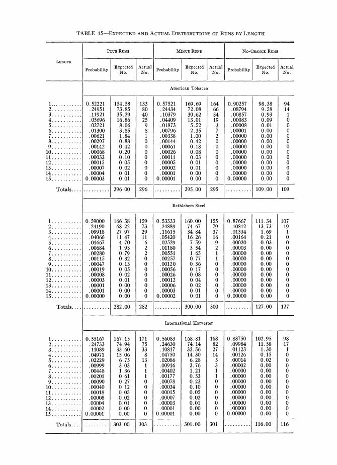
T A B L E 15-EXPECTED OF RUNSBY LENGTHAND ACTUALDISTRIBUTIONS
I I I
LENGTH Probability Expected Actual Probability Expected Actual Probability Expected Actual1 1 1 1 1No . No . N o No . No . No.
I American Tobacco
T o t a l s . . . . I . . / 29600 / 296 1 . . . ./ 295.00 1 295 . . . . . . . . ./ 109.00 1 109
I Bethlehem Steel
T o t a l s.
International Harvester
. .
.Totals ... . /. . . . . . .I 303.00 1 303 1 . . . . . . . . .I 301 00 I 301 I . . . . . . . . . ./ 116.00 1 116

83 BEHAVIOR OF STOCK-MARKET PRICES
and 111, however, Alexander goes on to test various other mechanical trading techniques, one of which involved a sim- plified form of the Dow theory. It turns out that most of these other techniques provide better profits than his filter tech- nique, and indeed better profits than buy-and-hold. This again led him to con- clude that the independence assumption of the random-walk model had been overturned.
Unfortunately a serious error remains, even in Alexander's latest computations. The error arises from the fact that he neglects dividends in computing profits for all of his mechanical trading rules. This tends to overstate the profitability of these trading rules relative to buy- and-hold. The reasoning is as follows. Under the buy-and-hold method the total profit is the price change for the time period plus any dividends that have been paid. Thus dividends act simply to increase the profitability of holding stock. All of Alexander's more complicated trading rules, however, involve short sales. In a short sale the borrower of the securities is usually required to reimburse the lender for any dividends that are paid while the short position is outstand- ing. Thus taking dividends into consid-eration will always tend to reduce the profitability of a mechanical trading rule relative to buy-and-hold. In fact, since in Alexander's computations the more com- plicated techniques are not substantially better than buy-and-hold, we would sus- pect that in most cases proper adjust- ment for dividends would probably com- pletely turn the tables in favor of the buy-and-hold method.
The above discussion would seem to raise grave doubts concerning the valid- ity of Alexander's most recent empirical results and thus of the conclusions he draws from these results. Because of the
complexities of the issues, however, these doubts cannot be completely or system- atically resolved within the confines of this paper. In a study now in progress various mechanical trading rules will be tested on data for individual securities rather than price indices. We turn now to a discussion of some of the preliminary results of this study.
Alexander's filter technique has been applied to the price series for the indi- vidual securities of the Dow- Jones Indus- trial Average used throughout this re-port. Filters from 0.5 per cent to 50 per cent were used. All profits were comput- ed on the basis of a trading block of 100 shares, taking proper account of divi-dends. That is, if an ex-dividend date occurs during some time period, the amount of the dividend is added to the net profits of a long position open during the period, or subtracted from the net profits of a short position. Profits were also computed gross and net of broker's commissions, where the commis- sions are the exact commissions on lots of 100 shares at the time of transaction. In addition, for purposes of comparison the profits before commissions from buy- ing and holding were computed for each security.
The results are shown in Table 16. Columns (1) and (2) of the table show average profits per filter, gross and net of commissions. Column (3) shows profits from buy-and-hold. Although they must be regarded as very preliminary, the re- sults are nevertheless impressive. We see in column (2) that, when commissions are taken into account, profits per filter are positive for only four securities. Thus, from the point of view of the average in- vestor, the results produced by the filter technique do not seem to invalidate the independence assumption of the random- walk model. In practice the largest prof-
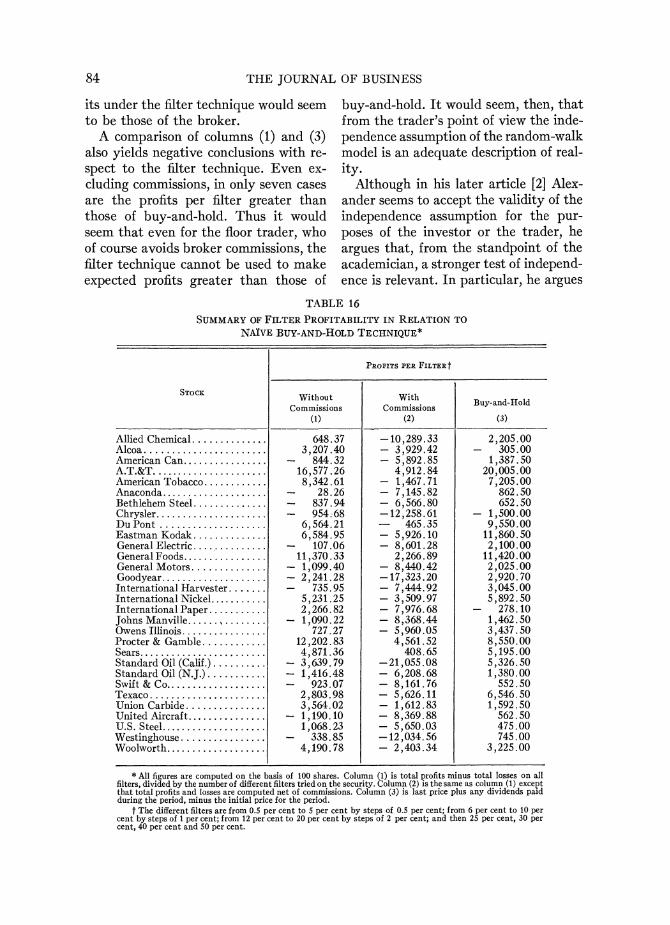
84 THE JOURNAL OF BUSINESS
its under the filter technique would seem buy.and.hold . It would seem, then. that to be those of the broker . from the trader's point of view the inde-
A comparison of columns (1) and (3) pendence assumption of the random-walk also yields negative conclusions with re- model is an adequate description of real- spect to the filter technique . Even ex- ity. cluding commissions. in only seven cases Although in his later article [2] Alex-are the profits per filter greater than ander seems to accept the validity of the those of buy.and.hold . Thus it would independence assumption for the pur- seem that even for the floor trader. who poses of the investor or the trader. he of course avoids broker commissions. the argues that. from the standpoint of the filter technique cannot be used to make academician. a stronger test of independ- expected profits greater than those of ence is relevant . In particular. he argues
TABLE 16 SUMMARYOF FILTERPROFITABILITY TOIN RELATION
N A ~ V E TECHNIQUE*BUY-AND-HOLD
I
Without Wi Commissions Commi
(2) I Allied Chemical . . . . . . . . . . . . . . Alcoa . . . . . . . . . . . . . . . . . . . . . . . American Can . . . . . . . . . . . . . . . . A.T.&T. . . . . . . . . . . . . . . . . . . . . . American Tobacco . . . . . . . . . . . . Anaconda . . . . . . . . . . . . . . . . . . . . Bethlehem Steel . . . . . . . . . . . . . . Chrysler . . . . . . . . . . . . . . . . . . . . . DuPont . . . . . . . . . . . . . . . . . . . . Eastman Kodak . . . . . . . . . . . . . . General Electric . . . . . . . . . . . . . . General Foods . . . . . . . . . . . . . . . . General Motors . . . . . . . . . . . . . . Goodyear . . . . . . . . . . . . . . . . . . . . International Harvester . . . . . . . International Nickel . . . . . . . . . . . International Paper . . . . . . . . . . . Johns Manville . . . . . ., . . . . . . . . Owens Illinois . . . . . . . . . . . . . . . . Procter & Gamble . . . . . . . . . . . . Sears. . . . . . . . . . . . . . . . . . . . . . . . Standard Oil (Calif.). . . . . . . . . .
.Standard Oil (N J.) . . . . . . . . . . . Swift & Co. . . . . . . . . . . . . . . . . . . Texaco . . . . . . . . . . . . . . . . . . . . . . Union Carbide . . . . . . . . . . . . . . . United Aircraft . . . . . . . . . . . . . . . U.S. Steel . . . . . . . . . . . . . . . . . . . . Westinghouse . . . . . . . . . . . . . . . . Woolworth. . . . . . . . . . . . . . . . . . .
"All fiqurcs s rc sumputc~l on tllt b ~ ~ i s I ) is totsl prufits minus tutsl l o s w on .illui 100 .Ilares . Column filters. ~livi;Ic:d 1)) the numberuf difTertnt filters trictlon t l r security .Culumn 2 is th::amc s: c-lumn I chie:;t that tutal prufits snd I ~ s c ssrc: cumpute~l net of sumnlis.ions . Colulnn .3) is lsst price plus any ilividenils p ~ i d during the period. minus the initial price for the period .
1.The different filters are from 0.5 per cent t o 5 per cent by steps of 0.5 per cent; from 6 per cent t o 10 per cent by steps of 1per cent; from 12 per cent to 20 per cent by steps of 2 per cent; and then 25 per cent, 30 per cent. 40 per cent and 50 per cent .

85 BEHAVIOR OF STOCK-MARKET PRICES
that the academic researcher is not in- terested in whether the dependence in series of price changes can be used to in- crease expected profits. Rather, he is primarily concerned with determining whether the independence assumption is an exact description of reality. In essence he proposes that we treat independence as a extreme null hypothesis and test it accordingly.
At this time we will ignore important counterarguments as to whether a strict test of an extreme null hypothesis is like- ly to be meaningful, given that for prac- tical purposes the hypothesis would seem to be a valid approximation to reality for both the statistician and the investor. We simply note that a signs test applied to the profit figures in column (1) of Table 16 would not reject the extreme null hypothesis of independence for any of the standard significance levels. Six- teen of the profit figures in column (1) are positive and fourteen are negative, which is not very far from the even split that would be expected under a pure ran- dom model without trends in the price levels. If we allowed for the long-term upward bias of the market, the results would conform even more closely to the predictions of the strict null hypothesis. Thus the results produced by the filter technique do not seem to overturn the independence assumption of the random- walk model, regardless of how strictly that assumption is interpreted.
Finally, we emphasize again that these results must be regarded as preliminary. Many more complicated analyses of the filter technique are yet to be completed. For example, although average profits per filter do not compare favorably with buy-and-hold, there may be particular filters which are consistently better than buy-and-hold for all securities. We pre- fer, however, to leave such issues to a
later paper. For now suffice it to say that preliminary results seem to indicate that the filter technique does not overturn the independence assumption of the random- walk model.
D. DISTRIBUTION OF SUCCESSORS
TO LARGE VALUES
Mandelbrot 137, pp. 418-191 has sug- gested that one plausible form of de-pendence that could partially account for the long tails of empirical distribu- tions of price changes is the following: Large changes may tend to be followed by large changes, but of random sign, whereas small changes tend to be fol- lowed by small changes.36 The economic rationale for this type of dependence hinges on the nature of the information process in a world of uncertainty. The hypothesis implicitly assumes that when important new information comes into the market, it cannot always be evalu- ated precisely. Sometimes the immediate price change caused by the new informa- tion will be too large, which will set in motion forces to produce a reaction. In other cases the immediate price change will not fully discount the information, and impetus will be created to move the price again in the same direction.
The statistical implication of this hy- pothesis is that the conditional probabil- ity that tomorrow's price change will be large, given that today's change has been large, is higher than the unconditional probability of a large change. To test this, empirical distributions of the imme- diate successors to large price changes have been computed for the daily differ-
Although the existence of this type of price be- havior could not be used by the investor to increase his expected profits, the behavior does fit into the statistical definition of dependence. That is, knowl- edge of today's price change does condition our pre- diction of the size, if not the sign, of tomorrow's change.

86 THE JOURNAL OF BUSINESS
ences of ten stocks. Six of the stocks were quency distributions of all price changes. chosen at random. They include Allied I t shows for each stock the number and Chemical, American Can, Eastman Ko- relative frequency of observations in the dak, Johns Manville, Standard Oil of distribution of successors within given New Jersey, and U.S. Steel. The other ranges of the distribution of all price four were chosen because they showed changes. For example, the number in longer than average tails in the tests of column (1) opposite Allied Chemical in- Sections I11 and IV. A large daily price dicates that there are twenty-seven ob- change was defined as a change in log servations in the distribution of succes-price greater than 0.03 in absolute value. sors to large values that fall within the
The results of the computations are intersextile range of the distribution of shown in Table 17. The table is arranged all price changes for Allied Chemical. to facilitate a direct comparison between The number in column (6) opposite Al- the frequency distributions of successors lied Chemical indicates that twenty-to large daily price changes and the fre- seven observations are 55.1 per cent of
TABLE 17
Intersextile 1 2 Pe r Cent 1 1 Per Cent 1> 1 Per Cent 1 T o t a lStock
(1) (21 (31 4 ( 5 )
Number
Allied Chemical.. . . . 27 46 48 1 49 American Can.. . . . . 13 26 27 5 32 A.T.&T. . . . . . . . . . . . 4 12 14 2 16 Eastman Kodak. . . . 25 35 39 5 44 Goodyear . . . . . . . . . . 40 66 66 4 70 Johns Manville. . . . . 38 62 63 3 66 Sears . . . . . . . . . . . . . . 14 25 28 3 3 1 Standard Oil (N. J.) . . 11 18 18 2 20 United Aircraft. . . . . 49 78 84 4 88 U.S. Steel.. . . . . . . . . 14 2 7 3 1 5 36
Frequency
(6) --
( 7 ) (8) (9) ---- Expected frequency. Allied Chemical.. ...
0.6667 .5510
0.9600 .9388
0.9800 .9796
0.0200 .0204
American Can. . . . . . .4063 .8125 .8438 .I562 A.T.&T. . . . . . . . . . . . .2500 .7500 .8750 .I250 Eastman Kodak. . . . .5682 .7955 .8864 .I136 Goodyear. . . . . . . . . . Johns Manville. . . . .
.5714
.5758 .9429 .9394
.9429
.9545 .0571 .0455
Sears. . . . . . . . . . . . . . .4516 .8065 .9032 .0968 Standard Oil (N. J.). . United Aircraft.. . . .
.5500
.5568 .9000 ,8864
.9000
.9545 .I000 .0455
U.S. Steel.. . . . . . . . . 0.3889 0.7500 0.8611 0.1389
* Number and freouencv of observations in the distributions of successors within given ranges of the distributions oi'all chanacs. The ranges arc defined as folloks: Intersestilt ='o 8; f r d i i -0.1; fractilc: 2 pcr ccnt = 0.98fractilt --0.02fractile; 1 per cent = 0.99fract1lt - 4 . 0 1 fracjilc. The fractiles arc the fractilcs of the distributions of all price changes and not of the distrlbut~ons of successors t o large changes.

87 BEHAVIOR OF STOCK-MARKET PRICES
the total number of successors to large values, whereas the distribution of all price changes contains, by definition, 66.7 per cent of its observations within its intersextile range. Similarly, the num- ber in column (9) opposite Goodyear indicates that in the distribution of suc- cessors 5.7 per cent of the observations fall outside of the 1 per cent range, whereas by definition only 2 per cent of the observations in the distribution of all changes are outside this range.
It is evident from Table 17 that the distributions of successors are flatter and have longer tails than the distributions of all price changes. This is best illus- trated by the relative frequencies. In every case the distribution of successors has less relative frequency within each fractile range than the distribution of all changes, which implies that the distribu- tion of successors has too much relative frequency outside these ranges.
These results can be presented graphi- cally by means of simple scatter dia- grams. This is done for American Tele- phone and Telegraph and Goodyear in Figure 8. The abscissas of the graphs show XI, the value of the large price change. The ordinates show Xz, the price change on the day immediately following a large change. Though it is diEcult to make strong statements from such graphs, as would be expected in light of Table 17, it does seem that the successors do not concentrate around the abscissas of the graphs as much as would be ex- pected if their distributions were the same as the distributions of all changes. Even a casual glance a t the graphs shows, however, that the signs of the successors do indeed seem to be random. Moreover, these statements hold for the graphs of the securities not included in Figure 8.
In sum, there is evidence that large changes tend to be followed by large
changes, but of random sign. However, though there does seem to be more bunching of large values than would be predicted by a purely independent mod- el, the tendency is not very strong. In Table 17 most of the successors to large observations do fall within the intersex- tile range even though more of the suc- cessors fall into the extreme tails than would be expected in a purely random model.
E. SUMMARY
None of the tests in this section give evidence of any important dependence in the first differences of the logs of stock prices. There is some evidence that large changes tend to be followed by large changes of either sign, but the depend- ence from this source does not seem to be too important. There is no evidence at all, however, that there is any depend- ence in the stock-price series that would be regarded as important for investment purposes. That is, the past history of the series cannot be used to increase the investor's expected profits.
It must be emphasized, however, that, while the observed departures from inde- pendence are extremely slight, this does not mean that they are unimportant for every conceivable purpose. For example, the fact that large changes tend to be followed by large changes may not be in- formation which yields profits to chart readers; but it may be very important to the economist seeking to understand the process of price determination in the capital market. The importance of any observed dependence will always depend on the question to be answered.
VI. CONCLUSION
The purpose of this paper has been to test empirically the random-walk model of stock price behavior. The model makes

American Tel. & Tel.
Goodyear
89 BEHAVIOR OF STOC K-MARKET PRICES
two basic assumptions: (1) successive price changes are independent, and (2) the price changes conform to some prob- ability distribution. We begin this sec- tion by summarizing the evidence con- cerning these assumptions. Then the im- plications of the results will be discussed from various points of view.
A. DISTRIBUTION OF PRICE CHANGES
In previous research on the distribu- tion of price changes the emphasis has been on the general shape of the distri- bution, and the conclusion has been that the distribution is approximately Gauss- ian or normal. Recent findings of Benoit Mandelbrot, however, have raised serious doubts concerning the validity of the Gaussian hypothesis. In particular, the Mandelbrot hypothesis states that em-pirical distributions of price changes con- form better to stable Paretian distribu- tions with characteristic exponents less than 2 than to the normal distribution (which is also stable Paretian but with characteristic exponent exactly equal to 2). The conclusion of this paper is that Mandelbrot's hypothesis does seem to be supported by the data. This conclusion was reached only after extensive testing had been carried out. The results of this testing will now be summarized.
If the Mandelbrot hypothesis is cor- rect, the empirical distributions of price changes should have longer tails than does the normal distribution. That is, the empirical distributions should contain more relative frequency in their extreme tails than would be expected under a simple Gaussian hypothesis. In Section I11frequency distributions were comput- ed for the daily changes in log price of each of the thirty stocks in the sample. The results were quite striking. The em- pirical distribution for each stock con-tained more relative frequency in its cen-
tral bell than would be expected under a normality hypothesis. More important, however, in every case the extreme tails of the distributions contained more rela- tive frequency than would be expected under the Gaussian hypothesis. As a further test of departures from normal- ity, a normal probability graph for the price changes of each stock was also ex- hibited in Section 111. As would be ex- pected with long-tailed frequency distri- butions, the graphs generally assumed the shape of an elongated S.
In an effort to explain the departures from normality in the empirical fre-quency distributions, two simple compli- cations of the Gaussian model were dis- cussed and tested in Section 111. One in- volved a variant of the mixture of distri- butions approach and suggested that perhaps weekend and holiday changes come from a normal distribution, but with a higher variance than the distribu- tion of daily changes within the week. The empirical evidence, however, did not support this hypothesis. The second ap- proach, a variant of the non-stationarity hypothesis, suggested that perhaps the leptokurtosis in the empirical frequency distributions is due to changes in the mean of the daily differences across time. The empirical tests demonstrated, how- ever, that the extreme values in the frequency distributions are so large that reasonable shifts in the mean cannot adequately explain them.
Section IV was concerned with testing the property of stability and developing estimates of the characteristic exponent a of the underlying stable Paretian proc- ess. It was emphasized that rigorously established procedures for estimating the parameters of stable Paretian distribu- tions are practically unknown because for most values of the characteristic ex- ponent there are no known, explicit

90 THE JOURNAL OF BUSINESS
expressions for the density functions. As a result there is virtually no sampling theory available. It was concluded that at present the only way to get satisfac- tory estimates of the characteristic ex- ponent is to use more than one estimat- ing procedure. Thus three different techniques for estimating a were dis-cussed, illustrated, and compared. The techniques involved double-log-normal- probability graphing, sequential compu- tation of variance, and range analysis. In a very few cases a seemed to be so close to 2 that it was indistinguishable from 2 in the estimates. In the vast majority of cases, however, the estimated values were less than 2, with some dispersion about an average value close to 1.90. On the basis of these estimates of a and the re- sults produced by the frequency distribu- tions and normal probability graphs, it was concluded that the Mandelbrot hy- pothesis fits the data better than the Gaussian hypothesis.
33. INDEPENDENCE
Section V of this paper was concerned, with testing the validity of the independ- ence assumption of the random-walk model on successive price changes for differencing intervals of one, four, nine, and sixteen days. The main techniques used were a serial correlation model, runs analysis, and -4lexander's filter tech-nique. For all tests and for all differenc- ing intervals the amount of dependence in the data seemed to be either extremely slight or else non-existent. Finally, there was some evidence of bunching of large values in the daily differences, but the degree of bunching seemed to be only slightly greater than would be expected in a purely random model. On the basis of all these tests it was concluded that the independence assumption of the ran- dom-walk model seems to be an adequate description of reality.
C. IMPLICATIONS OF INDEPENDENCE
We saw in Section I1 that a situation where successive price changes are inde- pendent is consistent with the existence of an "efficient" market for securities, that is, a market where, given the available information, actual prices at every point in time represent very good estimates of intrinsic values. We also saw that two factors that could possibly contribute to- ward establishing independence are (1) the existence of many sophisticated chart readers actively competing with each other to take advantage of any depend- encies in series of price changes, and (2) the existence of sophisticated analysts, where sophistication implies an ability both to predict better the occurrence of economic and political events which have a bearing on prices and to evaluate the eventual effects of such events on prices.
If his activities succeed in hdping to establish independence of successive price changes, then the sophisticated chart reader has defeated his own purposes. When successive price changes are inde- pendent, there can be no chart-reading technique which makes the expected profits of the investor greater than they would be under a naive buy-and-hold model. Such dogmatic statements do not apply to superior intrinsic value analysis, however. People who can consistently predict the occurrence of important events and evaluate their effects on prices will usually make larger profits than people who do not have this talent. The fact that the activities of these su- perior analysts help to make successive price changes independent does not imply that their expected profits cannot be greater than those of the investor who follows a buy-and-hold policy.
Of course, in practice, identifying peo- ple who qualify as superior analysts is not an easy task. The simple criterion

91 BEHAVIOR OF STOCK-MARKET PRICES
put forth in Section I1was the following: A superior analyst is one whose gains over many periods of time are consistently greater than those of the market. There are many institutions and individuals that claim to meet this criterion. In a separate paper their claims will be sys- tematically tested. We present here some of the preliminary results for open-end mutual funds.37
In their appeals to the public, mutual funds usually make two basic claims: (1) because it pools the resources of many individuals, a fund can diversify much more effectively than the average small investor; and (2) because of its manage- ment's closeness to the market, the fund is better able to detect "good buys" in individual securities. In most cases the first claim is probably true. The second, however, implies that mutual funds pro- vide returns higher than those earned by the market as a whole. It is this second claim that we now wish to test.
The return earned by the "market" during any time period can be measured in various ways. One possibility has been extensively explored by Fisher and Lorie [16] in a recent issue of this Journal. The basic assumption in all their computa- tions is that a t the beginning of each period studied the investor puts an equal amount of money in each common stock listed a t that time on the New York Stock Exchange. Different rates of return for the period are then computed for different possible tax brackets of the in- vestor, first under the assumption that all dividends are reinvested in the month paid and then under the assumption that dividends are not reinvested. All compu- tations include the relevant brokers' commissions. Following the Lorie-Fisher
37 The preliminary results reported below were prepared as an assigned term paper by one of my students, Gerhard T. Roth. The data source for all the calculations was Wiesenberger [24].
procedure, a tax-exempt investor who initially entered the market at the end of 1950 and reinvested subsequent divi- dends in the securities paying them would have made a compound annual rate of return of 14.7 per cent upon disinvesting his entire portfolio at the end of 1960.
Similar computations have been car-ried out for thirty-nine open-end mutual funds. The funds studied have been chosen on the following basis: (1) the fund was operating during the entire period from the end of 1950 through the end of 1960; and (2) no more than 5 per cent of its total assets were invested in bonds at the end of 1960. It was assumed that the investor put $10,000 into each fund at the end of 1950, reinvested all subsequent dividend distributions, and then cashed in his portfolio a t the end of 1960. It was also assumed, for sim- plicity, that the investor was tax exempt.
For our purposes, two different types of rates of return are of interest, gross and net of any loading charges. Most funds have a loading charge of about 8 per cent on new investment. That is, on a gross investment of $10,000 the inves- tor receives only about $9,200 worth of the fund's shares. The remainng $800 is usually a straight salesman's commis- sion and is not available to the fund's management for investment. From the investor's point of view the relevant rate of return on mutual funds to compare with the "market" rate is the return gross of loading charges, since the gross sum is the amount that the investor allo- cates to the funds. It is also interesting, however, to compute the yield on mutual funds net of any loading changes, since the net sum is the amount actually avail- able to management. Thus the net return is the relevant measure of management's performance in relation to the market.
For the period 1950-60 our mutual- fund investments had a gross return of

92 THE JOURNAI
14.1 per cent which is below the 14.7 per cent earned by the "market," as defined by Fisher and Lorie. The return, net of loading charges, on the mutual funds was 14.9 per cent, slightly but not sig- nificantly above the "market" return. Thus it seems that, at least for the period studied, mutual funds in general did not .do any better than the market.
Although mutual funds taken together do no better than the market, in a world of uncertainty, during any given time period some funds will do better than the market and some will do worse. When a Fund does better than the market during some time period, however, this is not necessarily evidence that the fund's man- agement has knowledge superior to that of the average investor. A good showing during a particular period may merely be a chance result which is, in the long run, balanced by poor showings in other peri- ods. It is only when a fund consistently does better than the market that there is any reason to feel that its higher than average returns may not be the work of lady luck.
In an effort to examine the consistency of the results obtained by different funds across time two separate tests were car- ried out. First, the compound rate of return, net of loading charges, was com- puted for each fund for the entire 1950- 60 period. Second, the return for each fund for each year was computed accord- ing to the formula
where Pit is the price of a share in fund j at the end of year t, pj, t+l is the price at the end of year t + 1, and dj, are the dividends per share paid by the fund during year t + 1. For each year the returns on the different funds were then
OF BUSINESS
ranked in ascending order, and a number from 1 to 39 was assigned to each.
The results are shown in Table 18. The order of the funds in the table is according to the return, net of loading charges, shown by the fund for the period 1950-60. This net return is shown in column (1). Columns (2)-(11) show the relative rankings of the year-by-year returns of each fund.
The most impressive feature of Table 18 is the inconsistency in the rankings of year-by-year returns for any given fund. For example, out of thirty-nine funds, no single fund consistently had returns high enough to place it among the top twenty funds for every year in the time period. On the other hand no single fund had returns low enough to place it among the bottom twenty of each year. Only two funds, Selected American and Equity, failed to have a return among the top ten for some year, and only three funds, Investment Corporation of America, Founders Mutual, and American Mu- tual, do not have a return among the bottom ten for some year. Thus funds in general seem to do no better than the market; in addition, individual funds do not seem to outperform consistently their corn petit or^.^^ Our conclusion, then, must be that so far the sophisticated analyst has escaped detection.
D. IMPLICATIONS OF THE MAN-
DELBROT HYPOTHESIS
The main conclusion of this paper with respect to the distribution of price changes is that a stable Paretian distri- bution with characteristic exponent a less than 2 seems to fit the data better
38 These results seem to be in complete agreement with those of Ira Horowitz 1221 and with the now famous "Study of Mutual Funds," prepared for the Securities and Exchange Commission by the Wharton School, University of Pennsylvania (87th Cong., 2d sess. [Washington, D.C.: Government Printing Office, 19621).

BEHAVIOR OF STOCK-MARKET PRICES 93
than the normal distribution. This con- 2 and a market dominated by a Gaussian clusion has implications from two points process is the following. In a Gaussian of view, economic and statistical, which market, if the sum of a large number of we shall now discuss in turn. price changes across some long time pe-
riod turns out to be very large, chances 1. ECONOMIC IMFLICATIONS are that each individual price change
The important difference between a during the time period is negligible when market dominated by a stable Paretian compared to the total change. In a mar- process with characteristic exponent a < ket that is stable Paretian with a < 2,
TABLE 18
YEAR-BY-YEARRANKING FUNDOF INDIVIDUALRETURNS
Keystone Lower Price. . T Rowe Price Growth. . Dreyfuss . . . . . . . . . . . . . . 18.4 37 37 14 3 7 11 3 2 3 7 Television Electronic.. . 18.4 21 4 9 2 33 20 16 2 4 20 NationalInvestors Corp. 18.0 3 35 4 19 27 4 5 5 8 1 DeVeghMutualFund.. 17.7 32 4 1 8 14 4 8 15 23 36 Growth Industries.. . . . 17.0 7 34 14 17 9 9 20 5 6 11 Massachusetts Investors
Growth . . . . . . . . . . . . .116.91 5 3 6 1 3 1 I 1 1 1 9 / 1 2 3 1 4 1 9 1 4 Franklin Custodian.. . . . 16.5 26 2 4 13 33 20 16 5 9 4 Investment Co. of Ameri-
ca . . . . . . . . . . . . . . . . . . 16.0 21 15 14 11 17 15 23 15 15 15 Chemical Fund, Inc.. . . 15.6 1 39 14 27 3 33 1 27 4 23 Founders Mutual. . . . . . 15.6 21 13 25 8 2 20 16 11 13 28 --- ~~~ ~ - -- ~ - ~
ton . . . . . . . . . . . . . . . . . 15.6 6 3 25 3 14 26 31 20 29 20 American Mutual.. . . . . 15.5 14 13 4 22 14 13 16 25 25 4 Keystone Growth.. . . . . 15.3 29 15 25 1 1 1 39 11 18 38 KeystoneHigh . . . . . . . . 15.2 10 7 3 27 23 36 5 27 25 11 AberdeenFund.. . . . . . . 15.1 32 23 9 25 9 7 10 27 7 30 Massachusetts Investors
Trust. . . . . . . . . . . . . . . Texas Fund, Inc.. . . . . . Eaton & Howard Stock. Guardian Mutual. . . . . . Scudder. Stevens. Clark. 1nvesto;s Stock eund. . . Fidelity Fund, Inc.. . . . . Fundamental Inv.. . . . . Century Shares.. . . . . . . Bullock Fund Ltd. . . . . . Financial Industries. . . . Group Common Stock. . Incorporated Investors. Equity Fund. . . . . . . . . . Selected American
Shares. . . . . . . . . . . . . . Dividend Shares. . . . . . . General Capital Corp.. . Wisconsin Fund. . . . . . . International Resources. Delaware Fund. . . . . . . . Hamilton Fund.. . . . . . . Colonial Energy. . . . . . .

94 THE JOURNAL OF BUSINESS
however, the size of the total will more than likely be the result of a few very large changes that took place during much shorter subperiods. In other words, whereas the path of the price level of a given security in a Gaussian market will be fairly continuous, in a stable Paretian market with a < 2 it will usually be dis- continuous. More simply, in a stable Paretian market with a < 2, the price of a security will often tend to jump up or down by very large amounts during very short time periods.39
When combined with independence of successive price changes, the discontinu- ity of price levels in a stable Paretian market may provide important insights into the nature of the process that gener- ates changes in intrinsic values across time. We saw earlier that independence of successive price changes is consistent with an "efficient" market, that is, a market where prices at every point in time represent best estimates of intrin- sic values. This implies in turn that, when an intrinsic value changes, the ac- tual price will adjust "instantaneously," where instantaneously means, among other things, that the actual price will initially overshoot the new intrinsic value as often as it will undershoot it.
In this light the combination of inde- pendence and a Gaussian distribution for the price changes would imply that in- trinsic values do not very often change by large amounts. On the other hand, the combination of independence and a stable Paretian distribution with a < 2 for the price changes would imply that intrinsic values often change by large amounts during very short periods of time-a situation quite consistent with a dynamic economy in a world of uncer-tainty.
38 For a proof of these statements see Darling 1131 or Anov and Bobnov 141.
The discontinuous nature of a stable Paretian market bas some more practical implications, however. The fact that there are a large number of abrupt changes in a stable Paretian market means that such a market is inherently more risky than a Gaussian market. The variability of a given expected yield is higher in a stable Paretian market than it would be in a Gaussian market, and the probability of large losses is greater.
Moreover, in a stable Paretian market with a < 2 speculators cannot usually protect themselves from large losses by means of such devices as "stop-loss" or-ders. If the price level is going to fall very much, the total decline will prob- ably be accomplished very rapidly, so that it may be impossible to carry out many "stop-loss" orders a t intermediate prices.
Finally, in some cases it may be pos- sible a posteriori to find "causal explana- tions" for specific large price changes in terms of more basic economic variables. If the behavior of these more basic vari- ables is itself largely unpredictable, how- ever, the "causal explanation'' will not be of much help in forecasting the appear- ance of large changes in the future. In addition it must be kept in mind that in the series we have been studying, there are very many large changes and the "explanations" are far from obvious. For example, the two largest changes in the Dow- Jones Industrial Average during the period covered by the data occurred on May 28 and May 29, 1962. Market ana- lysts are still trying to find plausible "ex- planations" for these two days.
2. STATISTICAL IMPLICATIONS
The statistical implications of the Mandelbrot hypothesis follow mostly from the absence of a finite variance for stable Paretian distributions with char-
95 BEHAVIOR OF STOCIK-MARKET PRICES
acteristic exponents less than 2. In prac- tical terms "infinite" variance means that the sample variance and standard deviation of a stable Paretian process with a < 2 will show extremely erratic behavior even for very large samples. That is, for larger and larger sample sizes the variability of the sample variance and standard deviation will not tend to dampen nearly as much as would be ex- pected with a Gaussian process. Because of their extremely erratic behavior, the sample variance and standard deviation are not meaningful measures of the vari- ability inherent in a stable Paretian process with a < 2.
This does not mean, however, that we are helpless in describing the dispersion of such a process. There are other meas- ures of variability, such as interfractile ranges and the mean absolute deviation, which have both finite expectation and much less erratic sampling behavior than the variance and standard deviation.40
Figure 9 presents a striking demon- stration of these statements. It shows the path of the sequential sample standard deviation and the sequential mean abso- lute deviation for four se~urities.~' The upper set of points on each graph repre- sents the path of the standard deviation, while the lower set represents the sample sequential mean absolute deviation. In
40 The mean absolute deviation is defined as
where x is the variable and N is the total sample size.
41 Sequential computation of a parameter means that the ct~mulativesequential sample value of the parameter is recomputed a t fixed intervals subse- quent to the beginning of the sampling period. Each new computation of the parameter in the sequence contains the same values of the random variable as the computation immediately preceding it, plus any new values of the variable that have since been generated.
every case the sequential mean absolute deviation shows less erratic behavior as the sample size is increased than does the sequential standard deviation. Even for very large samples the sequential stand- ard deviation often shows very large dis- crete jumps, which are of course due to the occurrence of extremely large price changes in the data. As the sample size is increased, however, these same large price changes do not have nearly as strong an effect on the sequential mean absolute deviation. This would seem to be strong evidence that for distributions of price changes the mean absolute deviation is a much more reliable estimate of variabil- ity than the standard deviation.
In general, when dealing with stable Paretian distributions with characteristic exponents less than 2, the researcher should avoid the concept of variance both in his empirical work and in any economic models he may construct. For example, from an empirical point of view, when there is good reason to believe that the distribution of residuals has in- finite variance, it is not very appealing to use a regression technique that has as its criterion the minimization of the sum of squared residuals from the regression line, since the expectation of that sum will be infinite.
This does not mean, however, that we are helpless when trying to estimate the parameters of a linear model if the vari- ables of interest are subject to stable Paretian distributions with infinite vari- ances. For example, an alternative tech- nique, absolute-value regression, involves minimizing the sum of the absolute val- ues of the residuals from the regression line. Since the expectation of the absolute value of the residual will be finite as long as the characteristic exponent a of the distribution of residuals is greater than 1, this minimization criterion is meaning-

- - -
--
96 THE JOURNAL OF BUSINESS
ful for a wide variety of stable Paretian p roce~ses .~~
A good example of an economic model which uses the notion of variance in situ- ations where there is good reason to be- lieve that variances are infinite is the classic Markowitz [39]analysis of efficient portfolios. In Markowitz' terms, efficient portfolios are portfolios which have max-
42 For a discussion of the technique of absolute value regression see Wagner [46], [47]. Wise [49]has shown that when the distribution of residuals has characteristic exponent 1 < a < 2, the usual least squares estimators of the parameters of a regression equation are consistent and unbiased. He has further
.085 AMERlCbN CAN
.020 ,
.015:
. ..
..:.''bhc%~-.-.010 :
,005
.ooo. 300 600 900 1860
,025 GEN. MOTORS
.C.20.
.015 .
? \,*A*
,005
. 000 400 800 1200
?..---
imum expected return for given variance of expected return. If yields on securities follow distributions kith infinite vari-ances, however, the expected yield of a diversified portfolio will also follow a
shown, however, that when a < 2, the least squares estimators are not the most efficient linear esti- mators, i.e., there are other techniques for which the sampling distributions of the regression parame- ters have lower dispersion than the sampling distri- butions of the least squares estimates. Of course i t is also possible that some non-linear technique, such as absolute value regression, provides even more efficient estimates than the most efficient linear estimators.
. oes A. T. AND T.
.020
-.015
.010. -.t:
.005 ;..,;$ 'L-.4 .----.w
."O'lj 300 600 900 1200
.095 SEARS
.020.
.015
,--
300 600 900 1200
FIG. 9.-Sequential standard deviations and sequential mean absolute deviations. Horizontal axes show sequential sample sizes; vertical axes show parameter estimates.

97 BEHAVIOR OF STOCK-MARKET PRICES
distribution with an infinite variance. In this situation the mean-variance concept of an efficient portfolio loses its meaning.
This does not mean, however, that diversification is a meaningless concept in a stable Paretian market, or that it is impossible to develop a model for port- folio analysis. In a separate paper [IS] this author has shown that, if concepts of variability other than the variance are used, it is possible to develop a model for portfolio analysis in a stable Paretian market. I t is also possible to define the conditions under which increasing diver- sification has the effect of reducing the dispersion of the distribution of the re- turn on the portfolio, even though the variance of that distribution may be in- finite.
Finally, although the Gaussian or nor- mal distribution does not seem to be an adequate representation of distributions of stock price changes, it is not neces- sarily the case that stable Paretian dis- tributions with infinite variances provide the only alternative. It is possible that there are long-tailed distributions with finite variances that could also be used to describe the data.43 We shall now argue, however, that one is forced to accept many of the conclusions discussed above, regardless of the position taken with re- spect to the finite-versus-infinite-vari-ance argument.
For example, although one may feel that it is nonsense to talk about infinite variances when dealing with real-world variables, one is nevertheless forced to admit that for distributions of stock price changes the sampling behavior of the standard deviation is much more erratic than that of alternative dispersion pa-
43 It is important to note, however, that stable Paretian distributions with characteristic exponents less than 2 are the only long-tailed distributions that have the crucial property of stability or invari- ance under addition.
rameters such as the mean absolute de- viation. For this reason it may be better to use these alternative dispersion pa- rameters in empirical work even though one may feel that in fact all variances are finite.
Similarly, the asymptotic properties of the parameters in a classical least- squares regression analysis are strongly dependent on the assumption of finite variance in the distribution of the resid- uals. Thus, if in some practical situation one feels that this distribution, though long-tailed, has finite variance, in prin- ciple one may feel justified in using the least-squares technique. If, however, one observes that the sampling behavior of the parameter estimates produced by the least-squares technique is much more erratic than that of some alternative technique, one may be forced to conclude that for reasons of efficiency the alterna- tive technique is superior to least squares.
The same sort of argument can be applied to the portfolio-analysis problem. Although one may feel that in principle real-world distributions of returns must have finite variances, it is well known that the usual Markowitz-type efficient set analysis is highly sensitive to the estimates of the variances that are used. Thus, if it is difficult to develop good estimates of variances because of erratic sampling behavior induced by long-tailed distributions of returns, one may feel forced to use an alternative measure of dispersion in portfolio analyses.
Finally, from the point of view of the individual investor, the name that the researcher gives to the probability dis- tribution of the return on a security is irrelevant, as is the argument concerning whether variances are finite or infinite. The investor's sole interest is in the shape of the distribution. That is, the only in- formation he needs concerns the proba-

98 THE JOURNAL OF BUSINESS
bility of gains and losses greater than given amounts. As long as two different hypotheses provide adequate descriptions of the relative frequencies, the investor is indifferent as to whether the researcher tells him that distributions of returns are stable Paretian with characteristic expo- nent a < 2 or just long-tailed but with finite variances.
In essence, all of the above arguments merely say that, given the long-tailed empirical frequency distributions that have been observed, in most cases one's subsequent behavior in light of these results will be the same whether one leans toward the Mandelbrot hypothesis or to- ward some alternative hypothesis involv- ing other long-tailed distributions. For most purposes the implications of the empirical work reported in this paper are independent of any conclusions concern- ing the name of the hypothesis which the data seem to support.
E. POSSIBLE DIRECTIONS FOR
FUTURE RESEARCH
It seems safe to say that this paper has presented strong and voluminous evidence in favor of the random-walk hypothesis. In business and economic re- search, however, one can never claim to have established a hypothesis beyond question. There are always additional tests which would tend either to confirm the validity of the hypothesis or to con- tradict results previously obtained. In the final paragraphs of this paper we wish to suggest some possible directions which future research on the random- walk hypothesis could take.
1. ADDITIONAL POSSIBLE TESTS
OF DEPENDENCE
There are two different approaches to testing for independence. First, one can carry out purely statistical tests. If these
tend to support the assumption of inde- pendence, one may then infer that there are probably no mechanical trading rules based on patterns in the past history of price changes which will make the profits of the investor greater than they would be under a buy-and-hold policy. Second, one can proceed by directly testing dif- ferent mechanical trading rules to see whether or not they do provide profits greater than buy-and-hold. The serial- correlation model and runs tests dis-cussed in Section V are representative of the first approach, while Alexander's fil- ter technique is representative of the second.
Academic research to date has tended to concentrate on the statistical ap-proach. This is true, for example, of the extremely sophisticated work of Granger and Morgenstern [19], Moore [41], Ken-dall[26], and others. Aside from Alexan- der's work [I], [2], there has really been very little effort by academic people to test directly the various chartist theories that are popular in the financial world. Systematic validation or invalidation of these theories would represent a real contribution.
2. POSSIBLE RESEARCH ON THE DISTRI-
BUTION OF PRICE CHANGES
There are two possible courses which future research on the distribution of price changes could take. First, until now most research has been concerned with simply finding statistical distributions that seem to coincide with the empirical distributions of price changes. There has been relatively little effort spent in ex- ploring the more basic processes that give rise to the empirical distributions. In essence, there is as yet no general model of price formation in the stock market which explains price levels and distribu- tions of price changes in terms of the

99 BEHAVIOR OF STOCK-MARKET PRICES
behavior of more basic economic vari- ables. Developing and testing such a model would contribute greatly toward establishing sound theoretical founda-tions in this area.
Second, if distributions of price changes are truly stable Paretian with character- istic exponent a < 2, then it behooves us to develop further the statistical theory of stable Paretian distributions. In par- ticular, the theory would be much ad- vanced by evidence concerning the sam- pling behavior of different estimators of the parameters of these distributions. Unfortunately, rigorous analytical sam- pling theory will be difficult to develop as long as explicit expressions for the density functions of these distributions are not known.
Using Monte Carlo techniques, how- ever, it is possible to develop an ap-proximate sampling theory, even though explicit expressions for the density func-
tions remain unknown. In a study now under way the series-expansion approxi- mation to stable Paretian density func- tions derived by Bergstrom [7] is being used to develop a stable Paretian random numbers generator. With such a random numbers generator it will be possible to examine the behavior of different esti- mators of the parameters of stable Pare- tian distributions in successive random samples and in this way to develop an approximate sampling theory. The same procedure can be used, of course, to develop sampling theory for many dif- ferent types of statistical tools.
In sum, it has been demonstrated that first differences of stock prices seem to follow stable Paretian distributions with characteristic exponent a < 2. An im-portant step which remains to be taken is the development of a broad range of statistical tools for dealing with these distributions.
REFERENCES
1. ALEXANDER,S. S. "Price Movements in Speculative Markets: Trends or Random Walks," Industrial Management Review, I1 (May, 1961), 7-26.
2. -. "Price Movements in Speculative Markets: Trends or Random Walks, No. 2" in PAUL H. COOTNER(ed.) [9], pp. 338-72.
3. ANDERSON,R. L. <'The Distribution of the Serial Correlation Coefficient," Arznals of Mathematical Statistics, XI11 (1942), 1-13.
4. ANOW,D. Z., and BOBNOV, A. A. "The EX- treme Members of Samples and Their Role in the Sum of Independent Variables," Theory of Probability and Its Applications, V (1960), 415-35.
5. BACHELIER,L. J. B. A. Le Jeu, la chance, et le hasard. Paris: E. Flammarion, 1914, chaps. xviii-xix.
6. -. Th&orie de la speculation. Paris:
Transformed Beta-Variables. New York: John Wiley & Sons, 1958.
9. COOTNER, (ed.). The Ra?zdom PAULH. Character of Stock Market Prices. Cam-bridge: M.I.T. Press, 1964. This is an excel- lent compilation of past work on random walks in stock prices. In fact it contains most of the studies listed in these references.
10. -. "Stock Prices: Random vs. Sys-tematic Changes," Industrial Management Review, I11 (Spring, 1962), 25-45.
11. COWLES,A. "A Revision of Previous Con- clusions Regarding Stock Price Behavior, Econometrica, XXVIII (October, 1960), 909-15.
12. COWLES, H. E. "Some AA., and JONES, Posteriori Probabilities in Stock Market Action, Econometrica, V (July, 1937), 280- 94.
DONALD.Gauthier-Villars, 1900. Reprinted in PAUL 13. DARLING, "The Influence of the H. COOTNER(ed.) [9], pp. 17-78.
7. BERGSTROY,H. "On Some Expansions of Stable Distributions," Arkiv for Matematik, I1 (1952), 375-78.
8. BLOY,GUNNAR.Statistical Estimates and
Maximum Term in the Addition of Inde- pendent Variables," Transactions of the American Mathematical Society, LXXIII (1952), 95-107.
14. FAMA,EUGENEF. "Mandelbrot and the

3 T H E J O U R N A L
Stable Paretian Hypothesis," Journal of Business, X X X V I (October, 1963), 420-29. FAMA, EUGENE F. "Portfolio Analysis in a Stable Paretian Market," Management Sci- ence (January, 1965). FISHER,L. and LORIE, J . H. , "Rates o f Re- turn on Investments in Common Stocks," Journal of Business, X X X V I I (January, 1964), 1-21. GNEDENKO, A. N . B . V . , and KOLMOGOROV, Limit Distributions for Sums of Independent Random Variables. Translated from Rus- sian b y K . L . CHUNG. Cambridge, Mass.: Addison-Wesley, 1954. GODPREY, MICHAEL D., GRANGER, CLIVE W . J . , and MORGENSTERN, OSKAR. " T h e Random W a l k Hypothesis o f Stock Market Behavior," Kyklos, X V I I (1964), 1-30. GRANGER, C . W . J., and MORGENSTERN, 0. "Spectral Analysis o f N e w Y o r k Stock Market Prices," K y klos, X V I (1963), 1-27. GUMBEL,E . J . Statistical Theory of Extreme Values and Some Practical Applications. Ap- plied Mathematics Series, No. 33, (Wash- ington, D.C.: National Bureau o f Stand- ards, February 12, 1954). H ~ L D , Statistical Theory with Engi- ANDERS. neering Applications. New Y o r k : John Wi ley & Sons, 1952. HOROWITZ,IRA. " T h e Varying (?) Quality o f Investment Trus t Management," Jour-nal of the American Statistical Association, LVI I I (December, 1963), 1011-32. IBRAGIMOV,I. A., and TCHERNIN, K . E. "On the Unimodality o f Stable Laws," Theory of Probability and Its Applications, IV (Moscow, 1959), 453-56. Investment Companies. New Y o r k : Arthur Wiesenberger & Co., 1961. KENDALL, M . G . The Advanced Theory of Statistics. London: C. Griffin & Co., 1948, p. 412.
. "The Analysis o f Economic Time- Series," Journal of the Royal Statistical So- ciety (Ser. A ) , X C V I (1953), 11-25. K I N G , BENJAMIN F. "The Latent Statistical Structure o f Security Price Changes," un-published Ph.D. dissertation, Graduate School o f Business, University o f Chicago, 1964. LARSON, ARNOLD B. "Measurement o f a Random Process in Futures Prices," Food Research Institute Studies, I (November, 1960), 313-24.
BUSINESS
LEVY, PAUL. Calcul des probabilitibs. Paris: Gauthier-Villars, 1925. L INTNER,JOHN. "Distribution o f Incomes o f Corporations among Dividends, Re-tained Earnings and Taxes," Papers and Proceedings of the American Economic Asso- ciation, X L V I ( M a y , 1956), pp. 97-113. MANDELBROT,BENOIT. " A Class o f Long- tailed Probability Distributions and the Empirical Distribution o f C i t y Sizes," Re-search note, Thomas J . Watson Research Center, Yorktown Heights, N.Y. , M a y 23, 1962.
. " N e w Methods in Statistical Eco- nomics," Journal of Political Economy, L X I (October, 1963), 421-40.
. "Paretian Distributions and In-come Maximization," Quarterly Journal of Economics, L X X V I (February, 1962), 57- 85.
. "The Pareto-LCvy Law and the Distribution o f Income," International Eco- nomic Review, I ( M a y , 1960), 79-106.
. "The Stable Paretian Income Dis- tribution when the Apparent Exponent Is Near Two," International Economic Review, IV (January, 1963), 111-14.
. "Stable Paretian Random Func- tions and the Multiplicative Variation of Income," Econometrics, X X I X (October, 1961), 517-43.
. " T h e Variation o f Certain Specula- tive Prices," Journal of Business, X X X V I (October, 1963), 394-419. MANDELBROT,BENOIT, and ZARNPALLER, FREDERICK. "Five Place Tables o f Cer- tain Stable Distributions," Research note, Thomas J . Watson Research Center, York - town Heights, N . Y . ,December 31, 1959. MARKOWITZ, HARRY. PortfDlio Selection: Eficient Diversification of Investments. New Y o r k : John Wi ley & Sons, 1959. MILLER, MERTON H., and MODIGLIANI, FRANCO. "Dividend Policy, Growth, and the Valuation o f Shares," Journal of Busi- ness, X X X I V (October, 1961), 41 1-33. MOORE, ARNOLD. " A Statistical Analysis o f Common-Stock Prices," unpublished Ph.D. dissertation, Graduate School o f Business, University o f Chicago, 1962. OSBORNE,M . F. M . "Brownian Motion in the Stock Market," Operations Research, V I I (March-April, 1959), 145-73.

101 BEHAVIOR OF STOCK-MARKET PRICES
43. ROBERTS,HARRY V. "Stock Market 'Pat- terns' and Financial Analysis: Methodo- logical Suggestions," Journal of Finance, XIV (March, 1959), 1-10.
44. TIPPET,L. H. C. "On the Extreme Indi- viduals and the Range of Samples Taken from a Normal Population," Biontetrika, XVII (1925), 364-87.
45. TUKEY,J. W. "The Future of Data Analy- sis," Annals of Mathematical Statistics, XXXIII (1962), 14-21.
46. WAGNER,H ~ R V E Y "LinearM. Program-ming Techniques for Regression Analysis," Journal of the A9nerica~z Statistical Associa- tion, LIV (1959), 206-12.
47. -. "Non-Linear Regression with Min- imal Assumptions," Jour~zal ofthe American Statistical Association, LVII (1962), 572-78.
48. WALLIS, W. A., and ROBERTS, H. V. Sta- tistics: A New Approach. Glencoe Ill. :Free Press, 1956.
49. WISE,JOHN. "Linear Estimators for Linear Regression Systems Having Infinite Vari- ances," paper presented a t the Berkeley- Stanford Mathematical Economics Semi- nar, October, 1963.
50. WORKING,H. "A Random Difference Series for Use in the Analysis of Time Series," Journal of tlze American Statistical Associa- tion, XXIX (March, 1934), 11-24.
APPENDIX
STATISTICAL THEORY OF STABLE PARETIAN DISTRIBUTIONS
A. STABLE PARETIAN DISTRIBUTIONS : DEFINITION AND PARAMETERS
The stable Paretian family of distributions is defined by the logarithm of its characteristic function which has the general form
log f ( t ) = log E(eiut)
= i6t - y / t j a[l+ iP(t/ 1 t 1 )w(t, a ) ], ( A l )
where u is the random variable, t is any real number, i is 4-1, and
Stable Paretian distributions have four pa- rameters, a , p, 6, and y. The parameter a is called the characteristic exponent of the distri- bution. I t determines the height of, or total probability contained in, the extreme tails of the distribution and can take any value in the interval 0 < a 5 2. When a = 2, the relevant stable Paretian distribution is the normal dis- tributione44When a is in the interval 0 < a < 2,
44 The logarithm of the characteristic function of a normal distribution is log fj(t) = ipt - (uz/2)t2. This is the log characteristic function of a stable Paretian distribution with parameters a = 2, 6 = M, and -y = us/2. The parameters p and ua are, of course, the mean and variance of the normal distri- bution.
the extreme tails of the stable Paretian distri- butions are higher than those of the normal distribution, and the total probability in the extreme tails is larger the smaller the value of a. The most important consequence of this is that the variance exists (i.e., is finite) only in the limiting case a = 2. The mean, however, exists as long as a >
The parameter fl is an index of skewness which can take any value in the interval -1 5 p 5 1. When /3 = 0, the distribution is sym- metric. When /? > 0, the distribution is skewed right (i.e., has a long tail to the right), and the degree of right skewness is larger the larger the value of 6. Similarly wheu < 0 the distribu- tion is skewed left, and the degree of left skew- ness is larger the smaller the value of P.
The parameter 6 is the location parameter of the stable Paretian distribution. When the characteristic exponent a is greater than 1, 6 is the expected value or mean of the distribu- tion. When a 5 1, however, the mean of the distribution is not defined. In this case 6 will be some other parameter (e.g., the median when p = 0), which will describe the location of the distribution.
Finally, the parameter y defines the scale of a stable Paretian distribution. For example, when a = 2 (the normal distribution), y is one- half the variance. When a < 2, ho~vever, the variance of the stable Paretian distribution is infinite. In this case there will be a finite pa- rameter y which defines the scale of the distri-
For a proof of these statements see Gnedenko and Kolmogorov [17], pp. 179-83,

102 T H E JOURNAL O F BUSlNESS
bution, but i t will not be the variance. For ex- ample, when a = 1,P = 0 (which is the Cauchy infinite. I n this case there will be a finite pa- rameter y which defines the scale of the distri- distribution), y is the semi-interquartile range (i.e., one-half of the 0.75 fractile minus the 0.25 fractile).
B. KEY PROPERTIES OF STABLE
PARETIAN DISTRIBUTIONS
The three most important properties of stable Paretian distributions are (1) the asymp- totically Paretian nature of the extreme tail areas, (2) stability or invariance under addition, and (3) the fact that these distributions are the only possible limiting distributions for sums of independent, identically distributed, random variables.
1. The law of Pareto.-LCvy [29] has shown that the tails of stable Paretian distributions follow a weak or asymptotic form of the law of Pareto. Tha t is,
and
where u is the random variable, and the con- stants U1and U z are defined b ~ 4 ~
From expressions (A3) and (A4) i t is possible to define approximate densities for the extreme tail areas of stable Paretian distributions. If a new function P(u) for the tail probabilities is defined by expressions (A3) and (A4), the den- sity functions for the asymptotic portions of the tails are given by
46The constants U1 and Uz can be regarded as scale parameters for the positive and negative tails of the distribution. The relative size of these two constants determines the value of B and thus the skewness of the distribution. If UZ is large relative to U1, the distribution is skewed left (i.e., P < O), and skewed right when U1 is large relative to Uz
Although i t has been proven that stable Paretian distributions are ~ n i m o d a l , ~ "closed expressions for the densities of the central areas of these distributions are known for only three cases, the Gaussian (a = 2), the Cauchy (a =
1, = 0), and the well-known coin-tossing case (a = 5, P = 1, 6 = 0 and y = 1). At this point this is probably the greatest weakness in the theory. Without density functions it is very difficult to develop sampling theory for the pa- rameters of stable Paretian distributions. The importance of this limitation has been stressed throughout this paper.48
2. Stability or invariance u d e v addition.- By definition, a stable Paretian distribution is any distribution that is stable or invariant under addition. Tha t is, the distribution of sums of independent, identically distributed, stable Paretian variables is itself stable Paretian and has the same form as the distribution of the individual summands. The phrase "has the same form" is, of course, an imprecise verbal expression for a precise mathematical property. A more rigorous definition of stability is given by the logarithm of the characteristic function of sums of independent, identically distributed, stable Paretian variables. The expression for this function is
n l o g f ( t ) = i ( n 6 ) t t
- ( n r ) i t ~ ~ [ l + i ~ ~ w ( t , a)], ( ~ 8
where n is the number of variables in the sum and log f(t) is the logarithm of the characteristic function for the distribution of the individual summands. Expression (A8) is the same as (Al), the expression for logf(t), except that the pa- rameters 6 (location) and y (scale) are multi- plied by n. That is, except for origin and scale,
(i.e., @ > 0). When U1 is zero the distribution has maximal left skewness. When UZ is zero, the distri- bution has maximal right skewness. These two lim- iting cases correspond, of course, to values of P of -1 and 1. When UI = UZ,P = 0, and the distribu- tion is symmetric.
47 Ibraginov and Tchernin [23].
48It should be noted, however, that Bergstrom [7]has developed a series expansion to approximate the densities of stable Paretian distributions. The potential use of the series expansion in developing sampling theory for the parameters by means of Monte Carlo methods is discussed in Section VI of this paper.

103 BEHAVIOR OF STOCK-MARKET PRICES
the distribution of the sums is exactly the same as the distribution of the individual summands. More simply, stability means that the values of the parameters a and 0 remain constant under addition.
The definition of stability is always in terms of independent, identically distributed random variables. It will now be shown, however, that any linear weighted sum of independent, stable Paretian variables with the same characteristic exponent a will be stable Paretian with the same value of a. I n particular, suppose we have n independent, stable Paretian variables, uj, j = 1, . . .,n. Assume further that the distribu- tions of the various ui have the same character- istic exponent a , but possibly different location, scale, and skewness parameters (aj, yj, and pj, j = 1, . . .,n). Let us now form a new variable, V, which is a weighted sum of the uj with con- stant weights pi, j = I,.. . .,n. The log charac- teristic function of V w~ l l then be
log F ( t ) = C l o g j i ( p i t ) 1=1
X l t ~ ~ [ l + i ~ < ~ w ( t ,a)],
where
and log fj(t) is the log characteristic function of uj. Expression (A9) is the log characteristic function of a stable Paretian distribution with characteristic exponent a and with location, scale, and skewness parameters that are weight- ed sums of the location, scale, and skewness parameters of the distributions of the uj.
3. Limiting distributions.-It can be shown that stability or invariance under addition leads to a most important corollary property of stable Paretian distributions; they are the only possible limiting distributions for sums of inde- pendent, identically distributed, random vari- ables.49 I t is well known that if such variables
49 For a proof see Gnedenko and Kolmogorov [Ill, pp. 162-63.
have finite variance the limiting distribution for their sum will be the normal distribution. If the basic variables have infinite variance, however, and if their sums follow a limiting dis- tribution, the limiting distribution must be stable Paretian with 0 < a < 2.
It has been proven independently by Gne- denko and Doeblin that, in order for the limit- ing distribution of sums to be stable Paretian with characteristic exponent a(0 < a < 2), it is necessary and sufficient that50
F ( - U ) -+ss u + m , ( A l l )1 - F ( u ) Cz
and for every constant k > 0,
where F is the cumulative distribution function of the random variable u and C1 and Ct are constants. Expressions (All) and (A12) will henceforth be called the conditions of Doeblin and Gnedenko.
I t is clear that any variable that is asymptot- ically Paretian (regardless of whether it is also stable) will satisfy these conditions. For such a variable, as u -+ a ,
and
and the conditions of Doeblin and Gnedenko are satisfied.
T o the best of my knowledge non-stable, asymptotically Paretian variables with expo- nent a < 2 are the only known variables of in- finite variance that satisfy conditions (All) and (A12). Thus they are the only known non-stable variables whose sums approach stable Paretian limiting distributions with character- istic exponents less than 2.
h0 For a proof see Gnedenko and Kolmogorov [17], pp. 175-80.
104 THE JOURNAL OF BUSINESS
C. PROPERTIES OF RANGES OF SUMS OF STABLE PARETIAN VARIABLES
By the definition of stability, sums of inde- pendent realizations of a stable Paretian vari- able are stable Paretian with the same value of the characteristic exponent a as the distribu- tion of the individual summands. The process of taking sums does, of course, change the scale or unit of measurement of the distribution.
Let us now pose the problem of finding a constant by which to weight each variable in the sum so that the scale parameter of the dis- tribution of sums is the same as that of the dis- tribution of the individual summands. This amounts to finding a constant, a, such that
Solving this expression for a we get
which implies that each of the summands must be divided by nila if the scale, or unit of meas- urement, of the distribution of sums is to be the same as that of the distribution of the indi- vidual summands. The converse proposition, of course, is that the scale of the distribution of unweighted sums is nila times the scale of the distribution of the individual summands. Thus, for example, the intersextile range of the dis- tribution of sums of n independent realizations of a stable Paretian variable will be nila times the intersextile range of the distribution of the individual summands. This property provides the basis of the range analysis approach to esti- mating a discussed in Section IV, C of this paper.51
D. PROPERTIES OF THE SEQUENTIAL VARIANCE
OF A STABLE PARETIAN VARIABLE
Let u be a stable Paretian random variable with characteristic exponent a < 2, and with location, scale, and skewness parameters 6, y, and p. Define a new variable, y = u - 6, whose distribution is exactly the same as that of u,
61 I t is worth noting that although the scale of the distribution of sums expands with n at the rate d l a , the scale parameter y expands directly with lz. Thus y itself represents some more basic scale pa- rameter raised to the power of a. For example, in the normal case (a = 2) y is related to the variance, but the variance is just the square of the standard deviation. The standard deviation, of course, is the more direct measure of the scale of the normal dis- tribution.
except that the location parameter has been set equal to 0.
Suppose now that we are interested in the probability distribution of y2. The positive tail of the distribution of y2 is related to the tails of the distribution of y in the following way:
But since the tails of the distribution of y follow an asymptotic form of the law of Pareto, for very large values of y this is just
Substituting C1 = Ui and C2= U; into ex-pression (A16) and simplifying we get
which is a Paretian expression with exponent a' = aj2 and scale parameter C'1 = C1+ C2.
The tail probabilities for the negative tail of the distribution of y2 are, of course, all identi- cally zero. This is 5quivalent to saying that the scale parameter, C2, in the Paretian expression for the negative tail of the distribution of y2 is zero.
Let us now turn our attention to the distri- bution of sums of independent realizations of the variable y2. Since y2 is asymptotically Pare- tian, it satisfies the conditions of Doeblin and Gnedenko, and thus sums of y2 will approach a stable Paretian distribution with characteristic exponent a' = a/2 and skewness
We know from previous discussions that, if the scale of the distribution of sums is to be the same as that of the distribution of j2, the sums must be scaled by n-lla' = n-2Ia, where n is the number of summands. Thus the distributions of
y 2and n - " Ci=l y 2 ( A 1 9 )
will be identical. This discussion provides us with a way to
analyze the distribution of the sample variance of the stable Paretian variable u. For values

105 BEHAVIOR OF STOCK-MARKET PRICES
of a less than 2, the population variance of the random variable u is infinite. The sample vari- ance of n independent realizations of u is
This can be multiplied by n-z1"+21a = 1with the result
Now we know that the distribution of
is stable Paretian and independent of n. In particular, the median (or any other fractile)
of this distribution has the same value for all n. This is not true, however, for the distribution of S2. The median or any other fractile of the distribution of S2 will grow in proportion to
For example, if ut is an independent, stable Paretian variable generated in time series, then the .ffractile of the distribution of the cumulative sample variance of ut a t time t l , as a function of the .ffractile of the distribu- tion of the sample variance a t time to is given by
where nl is the number of observations in the sample a t time tl, no is the number a t t, and S! and Si are the .f fractiles of the distribu- tions of the cumulative sample variances.
This result provides the basis for the sequen- tial variance approach to estimating a discussed in Section IV, D of this paper.

You have printed the following article:
The Behavior of Stock-Market PricesEugene F. FamaThe Journal of Business, Vol. 38, No. 1. (Jan., 1965), pp. 34-105.Stable URL:
http://links.jstor.org/sici?sici=0021-9398%28196501%2938%3A1%3C34%3ATBOSP%3E2.0.CO%3B2-6
This article references the following linked citations. If you are trying to access articles from anoff-campus location, you may be required to first logon via your library web site to access JSTOR. Pleasevisit your library's website or contact a librarian to learn about options for remote access to JSTOR.
[Footnotes]
5 Dividend Policy, Growth, and the Valuation of SharesMerton H. Miller; Franco ModiglianiThe Journal of Business, Vol. 34, No. 4. (Oct., 1961), pp. 411-433.Stable URL:
http://links.jstor.org/sici?sici=0021-9398%28196110%2934%3A4%3C411%3ADPGATV%3E2.0.CO%3B2-A
9 The Variation of Certain Speculative PricesBenoit MandelbrotThe Journal of Business, Vol. 36, No. 4. (Oct., 1963), pp. 394-419.Stable URL:
http://links.jstor.org/sici?sici=0021-9398%28196310%2936%3A4%3C394%3ATVOCSP%3E2.0.CO%3B2-L
10 The Future of Data AnalysisJohn W. TukeyThe Annals of Mathematical Statistics, Vol. 33, No. 1. (Mar., 1962), pp. 1-67.Stable URL:
http://links.jstor.org/sici?sici=0003-4851%28196203%2933%3A1%3C1%3ATFODA%3E2.0.CO%3B2-C
11 The Variation of Certain Speculative PricesBenoit MandelbrotThe Journal of Business, Vol. 36, No. 4. (Oct., 1963), pp. 394-419.Stable URL:
http://links.jstor.org/sici?sici=0021-9398%28196310%2936%3A4%3C394%3ATVOCSP%3E2.0.CO%3B2-L
http://www.jstor.org
LINKED CITATIONS- Page 1 of 6 -
NOTE: The reference numbering from the original has been maintained in this citation list.
15 The Variation of Certain Speculative PricesBenoit MandelbrotThe Journal of Business, Vol. 36, No. 4. (Oct., 1963), pp. 394-419.Stable URL:
http://links.jstor.org/sici?sici=0021-9398%28196310%2936%3A4%3C394%3ATVOCSP%3E2.0.CO%3B2-L
27 The Stable Paretian Income Distribution when the Apparent Exponent is Near TwoBenoit MandelbrotInternational Economic Review, Vol. 4, No. 1. (Jan., 1963), pp. 111-115.Stable URL:
http://links.jstor.org/sici?sici=0020-6598%28196301%294%3A1%3C111%3ATSPIDW%3E2.0.CO%3B2-X
28 The Variation of Certain Speculative PricesBenoit MandelbrotThe Journal of Business, Vol. 36, No. 4. (Oct., 1963), pp. 394-419.Stable URL:
http://links.jstor.org/sici?sici=0021-9398%28196310%2936%3A4%3C394%3ATVOCSP%3E2.0.CO%3B2-L
38 The Varying (?) Quality of Investment Trust ManagementIra HorowitzJournal of the American Statistical Association, Vol. 58, No. 304. (Dec., 1963), pp. 1011-1032.Stable URL:
http://links.jstor.org/sici?sici=0162-1459%28196312%2958%3A304%3C1011%3ATV%28QOI%3E2.0.CO%3B2-X
39 The Influence of the Maximum Term in the Addition of Independent Random VariablesD. A. DarlingTransactions of the American Mathematical Society, Vol. 73, No. 1. (Jul., 1952), pp. 95-107.Stable URL:
http://links.jstor.org/sici?sici=0002-9947%28195207%2973%3A1%3C95%3ATIOTMT%3E2.0.CO%3B2-I
42 Linear Programming Techniques for Regression AnalysisHarvey M. WagnerJournal of the American Statistical Association, Vol. 54, No. 285. (Mar., 1959), pp. 206-212.Stable URL:
http://links.jstor.org/sici?sici=0162-1459%28195903%2954%3A285%3C206%3ALPTFRA%3E2.0.CO%3B2-%23
http://www.jstor.org
LINKED CITATIONS- Page 2 of 6 -
NOTE: The reference numbering from the original has been maintained in this citation list.

42 Non-Linear Regression with Minimal AssumptionsHarvey M. WagnerJournal of the American Statistical Association, Vol. 57, No. 299. (Sep., 1962), pp. 572-578.Stable URL:
http://links.jstor.org/sici?sici=0162-1459%28196209%2957%3A299%3C572%3ANRWMA%3E2.0.CO%3B2-M
References
3 Distribution of the Serial Correlation CoefficientR. L. AndersonThe Annals of Mathematical Statistics, Vol. 13, No. 1. (Mar., 1942), pp. 1-13.Stable URL:
http://links.jstor.org/sici?sici=0003-4851%28194203%2913%3A1%3C1%3ADOTSCC%3E2.0.CO%3B2-G
11 A Revision of Previous Conclusions Regarding Stock Price BehaviorAlfred CowlesEconometrica, Vol. 28, No. 4. (Oct., 1960), pp. 909-915.Stable URL:
http://links.jstor.org/sici?sici=0012-9682%28196010%2928%3A4%3C909%3AAROPCR%3E2.0.CO%3B2-G
13 The Influence of the Maximum Term in the Addition of Independent Random VariablesD. A. DarlingTransactions of the American Mathematical Society, Vol. 73, No. 1. (Jul., 1952), pp. 95-107.Stable URL:
http://links.jstor.org/sici?sici=0002-9947%28195207%2973%3A1%3C95%3ATIOTMT%3E2.0.CO%3B2-I
14 Mandelbrot and the Stable Paretian HypothesisEugene F. FamaThe Journal of Business, Vol. 36, No. 4. (Oct., 1963), pp. 420-429.Stable URL:
http://links.jstor.org/sici?sici=0021-9398%28196310%2936%3A4%3C420%3AMATSPH%3E2.0.CO%3B2-F
http://www.jstor.org
LINKED CITATIONS- Page 3 of 6 -
NOTE: The reference numbering from the original has been maintained in this citation list.

15 Portfolio Analysis in a Stable Paretian MarketEugene F. FamaManagement Science, Vol. 11, No. 3, Series A, Sciences. (Jan., 1965), pp. 404-419.Stable URL:
http://links.jstor.org/sici?sici=0025-1909%28196501%2911%3A3%3C404%3APAIASP%3E2.0.CO%3B2-E
16 Rates of Return on Investments in Common StocksL. Fisher; J. H. LorieThe Journal of Business, Vol. 37, No. 1. (Jan., 1964), pp. 1-21.Stable URL:
http://links.jstor.org/sici?sici=0021-9398%28196401%2937%3A1%3C1%3AROROII%3E2.0.CO%3B2-T
22 The Varying (?) Quality of Investment Trust ManagementIra HorowitzJournal of the American Statistical Association, Vol. 58, No. 304. (Dec., 1963), pp. 1011-1032.Stable URL:
http://links.jstor.org/sici?sici=0162-1459%28196312%2958%3A304%3C1011%3ATV%28QOI%3E2.0.CO%3B2-X
32 New Methods in Statistical EconomicsBenoit MandelbrotThe Journal of Political Economy, Vol. 71, No. 5. (Oct., 1963), pp. 421-440.Stable URL:
http://links.jstor.org/sici?sici=0022-3808%28196310%2971%3A5%3C421%3ANMISE%3E2.0.CO%3B2-6
33 Paretian Distributions and Income MaximizationBenoit MandelbrotThe Quarterly Journal of Economics, Vol. 76, No. 1. (Feb., 1962), pp. 57-85.Stable URL:
http://links.jstor.org/sici?sici=0033-5533%28196202%2976%3A1%3C57%3APDAIM%3E2.0.CO%3B2-E
34 The Pareto-Lévy Law and the Distribution of IncomeBenoit MandelbrotInternational Economic Review, Vol. 1, No. 2. (May, 1960), pp. 79-106.Stable URL:
http://links.jstor.org/sici?sici=0020-6598%28196005%291%3A2%3C79%3ATPLATD%3E2.0.CO%3B2-O
http://www.jstor.org
LINKED CITATIONS- Page 4 of 6 -
NOTE: The reference numbering from the original has been maintained in this citation list.
35 The Stable Paretian Income Distribution when the Apparent Exponent is Near TwoBenoit MandelbrotInternational Economic Review, Vol. 4, No. 1. (Jan., 1963), pp. 111-115.Stable URL:
http://links.jstor.org/sici?sici=0020-6598%28196301%294%3A1%3C111%3ATSPIDW%3E2.0.CO%3B2-X
36 Stable Paretian Random Functions and the Multiplicative Variation of IncomeBenoit MandelbrotEconometrica, Vol. 29, No. 4. (Oct., 1961), pp. 517-543.Stable URL:
http://links.jstor.org/sici?sici=0012-9682%28196110%2929%3A4%3C517%3ASPRFAT%3E2.0.CO%3B2-Q
37 The Variation of Certain Speculative PricesBenoit MandelbrotThe Journal of Business, Vol. 36, No. 4. (Oct., 1963), pp. 394-419.Stable URL:
http://links.jstor.org/sici?sici=0021-9398%28196310%2936%3A4%3C394%3ATVOCSP%3E2.0.CO%3B2-L
40 Dividend Policy, Growth, and the Valuation of SharesMerton H. Miller; Franco ModiglianiThe Journal of Business, Vol. 34, No. 4. (Oct., 1961), pp. 411-433.Stable URL:
http://links.jstor.org/sici?sici=0021-9398%28196110%2934%3A4%3C411%3ADPGATV%3E2.0.CO%3B2-A
42 Brownian Motion in the Stock MarketM. F. M. OsborneOperations Research, Vol. 7, No. 2. (Mar. - Apr., 1959), pp. 145-173.Stable URL:
http://links.jstor.org/sici?sici=0030-364X%28195903%2F04%297%3A2%3C145%3ABMITSM%3E2.0.CO%3B2-0
43 Stock-Market "Patterns" and Financial Analysis: Methodological SuggestionsHarry V. RobertsThe Journal of Finance, Vol. 14, No. 1. (Mar., 1959), pp. 1-10.Stable URL:
http://links.jstor.org/sici?sici=0022-1082%28195903%2914%3A1%3C1%3AS%22AFAM%3E2.0.CO%3B2-H
http://www.jstor.org
LINKED CITATIONS- Page 5 of 6 -
NOTE: The reference numbering from the original has been maintained in this citation list.

45 The Future of Data AnalysisJohn W. TukeyThe Annals of Mathematical Statistics, Vol. 33, No. 1. (Mar., 1962), pp. 1-67.Stable URL:
http://links.jstor.org/sici?sici=0003-4851%28196203%2933%3A1%3C1%3ATFODA%3E2.0.CO%3B2-C
46 Linear Programming Techniques for Regression AnalysisHarvey M. WagnerJournal of the American Statistical Association, Vol. 54, No. 285. (Mar., 1959), pp. 206-212.Stable URL:
http://links.jstor.org/sici?sici=0162-1459%28195903%2954%3A285%3C206%3ALPTFRA%3E2.0.CO%3B2-%23
47 Non-Linear Regression with Minimal AssumptionsHarvey M. WagnerJournal of the American Statistical Association, Vol. 57, No. 299. (Sep., 1962), pp. 572-578.Stable URL:
http://links.jstor.org/sici?sici=0162-1459%28196209%2957%3A299%3C572%3ANRWMA%3E2.0.CO%3B2-M
50 A Random-Difference Series for Use in the Analysis of Time SeriesHolbrook WorkingJournal of the American Statistical Association, Vol. 29, No. 185. (Mar., 1934), pp. 11-24.Stable URL:
http://links.jstor.org/sici?sici=0162-1459%28193403%2929%3A185%3C11%3AARSFUI%3E2.0.CO%3B2-X
http://www.jstor.org
LINKED CITATIONS- Page 6 of 6 -
NOTE: The reference numbering from the original has been maintained in this citation list.