the bilateral and multilateral trade eﬀects of road … · even an increase of the joint railway...

The Bilateral and Multilateral Trade Effects of Road

and Railway Transport Infrastructure⋆

Peter Egger1 and Mario Larch2

1 Affiliation: Ifo Institute for Economic Research, Ludwig-Maximilian University of Munich, CESifo, and Centre

for Globalization and Economic Policy, University of Nottingham. Address: Ifo Institute for Economic

Research, Poschingerstrasse 5, 81679 Munich, Germany. E-mail: [email protected]

2 Affiliation: Ifo Institute for Economic Research and CESifo. Address: Ifo Institute for Economic Research,

Poschingerstrasse 5, 81679 Munich, Germany. E-mail: [email protected]

Abstract. Recent work by Anderson and van Wincoop (2003) emphasizes two insights innew-trade-theory-grounded empirical modeling of bilateral trade flows. First, the deter-minants of trade flows exert direct (first-order) bilateral as well as indirect (second-order)multilateral effects. The latter are referred to as ones of multilateral resistance. Second,full account of the impact of these determinants on bilateral trade can only be taken ina structural modeling approach. This paper analyzes the role of transport infrastructureendowments for bilateral trade along these lines. In particular, it pays attention to thepossible impact of the size of two countries’ road and railway infrastructure networks ontheir bilateral trade. We estimate a positive impact of these variables which varies acrosscountries due to the inherent non-linearity of the structural model. International tradeseems to respond to small expansions of the railway network more sensitively than to oneof the road network. However, marginal changes in transport infrastructure exert smalleffects on trade. Even an increase of the joint railway and road network size by ten percentraises intra-continental trade by less than one percent in the average country-pair.

Key words: Gravity model; Multilateral resistance; Transport infrastructure

JEL classification: F14; F15

⋆ Acknowledgements: To be added.

The Bilateral and Multilateral Trade Effects of Road and Railway Transport Infrastructure 1

1 Introduction

With interdependent countries, trade barriers and their alleviations exert direct effects

on bilateral trade as well as indirect ones on multilateral trade. Recently, Anderson and

van Wincoop (2003) establish a new-trade-theory-based empirical framework to account

for both of these effects in a structural modeling approach. The contribution of our paper

is the adoption of that framework for assessing whether and where, which and to what

extent transport infrastructure investments reduce trade costs and generate trade and

income effects. Paying particular attention to the size of two countries’ road and railway

infrastructure networks, we estimate their non-linear, dyad-specific impact on bilateral

and multilateral trade.

There is vast evidence on the broad interest of politicians on the matter. This interest

is shared by policy makers at the level of supranational organizations such as the World

Trade Organization (WTO), the Organization for Economic Cooperation and Develop-

ment (OECD), or the European Union (EU), but also at the level of national governments

in both the developed and the less developed part of the world. In comparison to the broad

political interest in the subject, the body of related academic research – and, in particu-

lar, of work in international economics – seems rather small. Trade economists conducted

transport-infrastructure-related work along two lines: establishing a theoretical and/or

empirical nexus between trade costs and transport infrastructure; and quantifying the

trade effects of (mostly transport) infrastructure on trade flows.

Theoretical work on the nexus between transport infrastructure and trade costs may

motivate the hypothesis about a negative relationship between the stock of transport

infrastructure and international trade costs (see Bougheas, Demetriades, and Morgenroth,

1999). However, multi-country models of trade suggest that direct positive effects may be

magnified but also offset through interdependence (see Bond, 2006, p. 484) since ”part of

the cost reductions due to transport investments will be passed on to the rest of the world


through changes in world prices.” Empirical evidence on that issue supports the view that

infrastructure investments reduce trade costs (Wilson, Mann, and Otsuki, 2004), but the

quantitative relationship seems to depend on other trade frictions – e.g., ones that are

geographical in nature (see Limao and Venables, 2001).

As long as transport infrastructure investments reduce trade costs, most trade models

predict that they increase trade. Evidence on trade enhancing effects of (broad or only

transport) infrastructure investments have been provided by Bougheas, Demetriades, and

Morgenroth (1999), Nordas and Piermartini (2004), Fujimura and Edmonds (2006), and

Francois and Manchin (2007).3 However, with many countries and heterogeneous bilat-

eral trade barriers even homogeneous changes in infrastructure investments will trigger

heterogeneous effects on bilateral trade in general equilibrium (see Anderson and van Win-

coop, 2003). Moreover, the effects of infrastructure will neither be linear nor log-linear.

And a simultaneous expansion in infrastructure network size may induce detrimental ef-

fects abroad (see Bond, 2006). These issues have not been taken into account in previous

empirical work.

It is this paper’s purpose to conduct a large-sample empirical analysis of the road and

railway network size effects on bilateral international trade flows. Unlike previous work,

we follow Anderson and van Wincoop’s (2003) seminal approach of modeling bilateral

trade flows by obeying structural interdependence of these flows via countries’ income con-

3 Bougheas, Demetriades, and Morgenroth (1999) estimate a gravity model of bilateral trade flows in a cross-

section of pairings of 9 European countries and find that, for instance, the length of the motor-way network has

a positive impact on the bilateral volume of trade. Nordas and Piermartini (2004) find a positive impact of al-

ternative transport and communication infrastructure indicators on bilateral trade in a cross-section of bilateral

trade flows among 138 countries. Fujimura and Edmonds (2006) estimate a significantly positive effect of road

infrastructure in a small panel of bilateral exports among seven members of the Mekong region (Cambodia,

Lao, Myanmar, Thailand, Vietnam, and two southern provinces of China) over the period 1981-2003. Pooling

cross-section data for pairings of 104 economies over 15 years from 1988 onwards, Francois and Manchin (2007)

estimate a positive significant impact of broad infrastructure (communications and transportation) on exports

which varies with per-capita income.


straints. This approach allows us to investigate not only the direct effects of infrastructure

investments, as is done in previous work, but also the indirect effects via explicit considera-

tion of countries’ interdependence. As we will show, associating the effects of infrastructure

investments only with their direct effects can lead to very misleading conclusions.

Since the bilateral world trade matrix contains numerous zero entries, we integrate the

approach of Anderson and van Wincoop (2003) in a pseudo-maximum likelihood Poisson

model as suggested by Santos Silva and Tenreyro (2006). Using the largest possible cross-

sectional data-set for which railway and road network size data are available – i.e., more

than 32, 000 country-pair dyads – we illustrate how country-pair-wise and also continent-

wise changes in road and railway transport infrastructure trigger heterogeneous effects on

trade across dyads and continents due to multilateral trade resistance. In particular, we

illustrate how identical percentage changes in road versus railway transport network size

affect bilateral trade flows differently. In this unified framework we may provide answers

about the whether and where, the which and to what extent moderate changes in transport

infrastructure affect bilateral trade.

The remainder of the paper is organized as follows. The next section briefly introduces

the estimation framework, closely following Anderson and van Wincoop (2003). Section

3 summarizes the testable hypotheses. Section 4 provides information about the sources

and features of the data and summarizes the estimation results. A quantification of the

impact of transport infrastructure on trade and welfare is provided in Section 5, and the

last section concludes with a summary of the major findings.


2 A gravity model with multilateral resistance and zero entries

in the bilateral trade matrix

We follow the theoretical approach of bilateral trade in an N -country, one-sector world

as in Anderson and van Wincoop (2003). Aggregate bilateral exports from country

i to country j (Xij) are described by a demand equation derived from a constant-

elasticity-of-substitution utility function. Anderson and van Wincoop use labels Yi, Yj,

and YW for exporter, importer, and world GDP, respectively. Additionally, they close the

model by ensuring that bilateral exports (including intra-national ones) add up to GDP

(∑N

j=1 Xij = Yi) and countries’ GDPs add up to world GDP (∑N

i=1 Yi =∑N

j=1 Yj = YW ).

Collecting k = 1, ..., K trade barrier variables into a product which weights these variables

by a corresponding set of (unknown) parameters (βk) and introducing two ’multilateral’

resistance (or consumer price) terms to be defined below, the multi-country new trade

theory model may be formulated as follows:

Xij =YiYj

YW

∏K

k=1 eβkDkij

P 1−σi P 1−σ

j

, (1)

where σ denotes the elasticity of substitution among different product varieties, Dkij is

the kth trade friction variable included in the model.4 P 1−σi and P 1−σ

j are referred to as

multilateral resistance terms, since they take the multilateral interdependence of trade

flows through country size and trade barriers into account. Anderson and van Wincoop

(2003) assume that trade frictions are symmetric in the sense that Dkij = Dkji for all

k = 1, ..., K, i, j = 1, ..., N . Then, they derive P 1−σi as a solution to the system of equations

P 1−σi =

N∑

j

[P σ−1

j θj

K∏

k=1

eβkDkji

]∀i, (2)

where θj = Yj/YW is country j’s fraction in world GDP. With positive bilateral exports

throughout, we may take the log of the dependent variable and formulate exports as a

4 One such variable is log bilateral distance between countries i and j. Other examples are indicator variables

such as common border or common official language between countries i and j. A complete list of all K trade

friction variables will be given in Section 4.1.


log-linear function of the determinants in (1) plus an error term. There, we may simply

enforce unitary GDP coefficients by subtracting (lnYi + ln Yj) from both sides of the

model. It is customary to replace YW by a constant.

However, with zero-inflated export data, taking logs leads to an excessive loss of obser-

vations. While this can be avoided in various ways, we follow Santos Silva and Tenreyro

(2006) by using the pseudo-maximum likelihood estimation method (PMLE). In par-

ticular, we will employ the Poisson PMLE and, alternatively, other generalized linear

models.5 Let us define the 1 × (K + L) vector of determinants in (1) in logs including

L fixed country effects for a country-pair ij as Zij. For all n observations, we have an

n × (K + L) matrix which we may refer to as Z. Furthermore, let the corresponding

(K + L) × 1 parameter vector be γ, and let us define the conditional mean of bilateral

exports as E[Xij|Zij] = g(Zγ). g(·) is a function which depends on the form of the chosen

distribution. We may use gij(Zijγ) or simply gij(·) with the element of g(·) for a single

country-pair. We can then specify the first-order conditions of a GLM version of the grav-

ity model in (1) as (see McCullagh and Nelder, 1989; Cameron and Trivedi, 1998, 2005;

Winkelmann, 2003):

N∑

i=1

N∑

j=1

[Xij − gij(·)]Zij = 0. (3)

With the Poisson PMLE model, gij(·) = exp(Zijγ) so that the first-order-conditions may

be expressed as

N∑

i=1

N∑

j=1

[Xij − exp(Zijγ)]Zij = 0. (4)

5 Generalized linear models (GLMs) are based on a distribution function of the linearized exponential family

which includes, for instance, the Gaussian, Poisson, negative binomial, or Gamma distributions. Note that (1)

can be estimated as a standard GLM as long as the assumed distribution function belongs to that family and

the multilateral resistance terms (5) are replaced by fixed exporter and importer effects (otherwise, the right-

hand-side of the model would be non-linear in the parameters). Given parameters based on GLM estimation

cum fixed effects, we can then solve for the multilateral resistance terms.


Given that the errors will be heteroskedastic with zero-inflated data, we should rely on

the Eicker-White sandwich estimator of the variance-covariance matrix for testing (see

Cameron and Trivedi, 2005).

Of course, zero trade flows need not only be accounted for with the dependent variable

but also with the design of the multilateral resistance terms. To illustrate this issue, let

us define an indicator variable I(Xji>0) which is unity if Xji > 0 and zero else. If Xij is

defined as in (1) with I(Xij>0) and zero else, it can easily be verified that (2) needs to be

modified to

P 1−σi =

N∑

j

[I(Xji>0)P

σ−1j θj

K∏

k=1

eβkDkji

]∀i. (5)

Hence, multilateral resistance only matters with non-zero bilateral trade flows.

3 Hypotheses

In terms of the empirical model of Section 2, infrastructure network size will affect trade

frictions and, accordingly, they will trigger direct and indirect effects on trade flows. From

a theoretical point of view, overland transport infrastructure such as the railway and road

network should increase international trade (Bougheas, Demetriades, and Morgenroth,

1999), especially trade among non-distant countries (Bond, 2006). The reason is that rail-

way and road transport infrastructure should primarily facilitate and lower the costs of

international goods transactions at reasonable distances (see also Limao and Venables,

2001).6 Accordingly, an empirical implementation of the model in equation (1) should ob-

tain positive parameter estimates for transport infrastructure variables, especially within

continents where goods can actually be transported across borders on railways or roads.

6 Bond (1997, p. 2) argues that road and railway networks will lower trade costs mainly between adjacent

countries ”but have little impact on transport costs with the rest of the world.”


The overall impact of road and railway network size on bilateral trade is composed of two

effects. The first one – a direct or first-order effect – is captured by the product∏

k eβkDkij

of trade friction variable effects in the nominator of equation (1). In case of a positive

impact of transport infrastructure on bilateral exports, the corresponding parameters βk

would be larger than zero. The second effect – an indirect or second-order effect – is

brought about by the multilateral resistance terms in the denominator of equation (1).

As can be see from the definition of these terms in equation (5), the indirect effect of a

variable Dkij (in our example, a transport infrastructure variable) will always be negative if

βk > 0. Hence, if several countries expand their railway and road infrastructure networks,

the impact on a given economy will be negative, if the indirect effects are larger than the

direct effect.

4 Empirical analysis

4.1 Data sources, features, and variable construction

Data on road and railway network size (which we refer to as transport infrastructure) are

available from the World Bank’s World Development Indicators 2005. Although there are

several years available from the late 1990s onwards, the time series for the infrastructure

variables contain missing values across periods for most of the countries, and the available

observations are unequally spaced over time. With multilateral resistance terms, even

randomly missing data on the right-hand-side of the model render exploitation of the time-

series variation in the data and the application of panel econometric methods infeasible.

However, the time variation in transport infrastructure data is relatively small, anyway.

Therefore, we compute averages over the years 1999-2003 for all variables and rely on

cross-section estimation throughout.


Nominal bilateral export flows in U.S. dollars are taken from the United Nation’s World

Trade Database. Nominal GDP in U.S. dollars is from the World Bank’s World Develop-

ment Indicators 2005. Other variables such as bilateral distance between two countries’

capitals7 and a set of indicator variables are based on information available from the

Centre d’Etudes Prospectives et d’Informations Internationales (CEPII; in particular, the

files geo cepii.xls and dist cepii.xls) and the World Trade Organization (WTO). The in-

dicator variables are the following: exporter/importer share a common official language,

exporter/importer have a common colonial relationship, exporter/importer have a recent

colonial relationship (for colonies after 1945), exporter/importer belong to the same coun-

try, exporter/importer are both landlocked, and exporter/importer are members of the

same regional trade agreement (customs unions, free trade areas, and other preferential

trade agreements as notified to the WTO).

The largest possible data-set for which the required information on the control variables is

available covers 180 economies, spanning a matrix of 180(180− 1) = 32, 220 international

bilateral relationships. Of those, 16, 854 (i.e., about 53 percent) have zero bilateral exports.

− Tables 1 and 2 −

Tables 1 and 2 provide further information about features of the data for the 32, 220

observations. For instance, average road network size is larger than average rail network

size by a factor of more than 24. In 15 percent of the international relationships the

exporter shares a common language with the importer. Only eight percent of the dyads

have (or form part of) a preferential trade agreement with preferential tariff liberalization

of the exporter against the importer and vice versa. With three percent of the pairs

both the exporter and the importer are landlocked. A minority of dyads had colonial

ties or needs to be classified as an intra-national relationship. According to Table 2 the

Americas have the largest transport infrastructure network across all continents. Europe

7 We use the great circle distance based on longitudes and latitudes of countries’ capitals.


is particularly well endowed with transport infrastructure, given its small geographical

extension.

Before turning to the econometric analysis of the impact of these variables on bilateral

(and multilateral) exports, we need to talk about variable construction. Most importantly,

we need to introduce the trade barrier variables collected in∏

k eβkDkij . In our model, each

of the six aforementioned indicator variables will enter in exponential form and represent

one trade friction variable Dkij. For instance, regional trade agreements would be captured

by eβRTA·RTAij . Also, the log of bilateral distance will enter as one such element in the form

eβDIST ·ln DISTij . Most importantly, we include joint road network size for an exporter and

an importer (as with bilateral distance, we use the functional form eβROAD·ln ROADij), and

similarly with joint rail network size. Finally, we include the number of ports and that

of airports to control for infrastructure effects associated with long-distance transport.

Hence, Dkij consists of eleven variables so that k = 1, ..., 11. However, it seems highly

implausible to assume that the joint road network matters for countries such as the United

States and Australia or Hungary and Japan (see Bond, 2006, for theoretical arguments).

Most of overall goods trade and even more so the one transported on roads and rails does

not cross continental borders. Accordingly, we assume that railway and road network size

only matters for intra-continental trade. Furthermore, we focus on effects of transport

infrastructure among countries excluding islands.

A first glance at the data suggests that there is a high correlation between the size of two

countries’ road and railway networks expressed in natural logarithms and log bilateral

exports. The partial correlation coefficient between exports and road network size is about

0.49 and that between exports and rail network size is about 0.37. Vast evidence on the role

of geographical proximity for bilateral trade points to a robust negative effect of distance

with an elasticity of about minus one. Given that, these simple correlation coefficients

indicate that transport infrastructure networks might mitigate the detrimental distance


effect on trade to a non-trivial extent. Of course, evidence based on partial correlation

coefficients is only preliminary (due to omitted variables and misspecified functional form

of infrastructure effects on trade), but the direction and possible size of the impact of

transport network size on bilateral trade calls for a structural investigation by means of

econometric analysis.

4.2 Estimation results

As indicated before, the data-set at hand contains a large amount of zeros which demands

for appropriate econometric methods such as the PMLE methods advocated by Santos

Silva and Tenreyro (2006) for gravity model estimation. We estimate all models with

exporter and importer fixed effects and subsequently solve for the multilateral resistance

terms which are consistent with the model parameter estimates. In Table 3, we summarize

the findings from three alternative estimation procedures. First, we estimate models along

the lines of Anderson and van Wincoop (2003) where we take the log of both sides of

equation (1) and include exporter and importer specific effects. Of course, this leads to a

loss of more than 50 percent of the observations and assumes that information of zero trade

flows is not informative. Second, we estimate a Poisson PMLE model based on the first-

order conditions in (4). Each of the procedures is estimated three times: (i) without any

infrastructure variables, (ii) including the road and railway infrastructure variables, and

(iii) including airports and ports in addition to road and railway infrastructure variables.8

8 In the Appendix, we report results for three alternative functional forms of the generalized linear model:

Gaussian PMLE, Gamma PMLE, and negative binomial PMLE. Gaussian PMLE is equivalent to an OLS

model with the right-hand-side variables in logs and the left-hand-side based on the level of exports. Gamma

PMLE is based on first-order conditions of the formPn

ij=1[Xij − exp(Zij γ)]exp(−Zij γ)Zij = 0 rather than

the ones given in (4), see Manning and Mullahy (2001). The negative binomial model is particularly suited

for cases with an over-dispersed Poisson distribution (see Cameron and Trivedi, 1998, or Winkelmann, 2003).

However, these models obviously perform poorly with the underlying data as compared to Poisson PMLE.


The results may be summarized in the following way. First, there is a dramatic difference

between the standard model in logs and the PMLE procedures. This indicates how harmful

it can be to ignore information contained in zeros in trade matrices. Most noteworthy,

road network size is significantly negative in the standard log-exports-based model but

significantly positive under PMLE. Also, the importance of both bilateral distance and

colonial relationships is overestimated with the standard approach. Regarding the model

characteristics, the explanatory power seems quite high across the board and the PMLE

models obviously work very well also in that regard.9

− Table 3 −

For estimation of the impact of a discrete change in road and railway network size, we

need to determine the multilateral resistance terms which are consistent with (5). With

the Poisson PMLE model, P 1−σi varies substantially across countries. Its mean is about

0.110, while its minimum and maximum values amount to 0.021 and 0.554, respectively.

5 Quantification of the role of rail and road transport

infrastructure networks for bilateral trade

To quantify the estimated effects, we increase road and railway network size (roads, rail-

ways, roads and railways) by ten percent for intra-continental dyads and compute the

trade effects associated with this change. Throughout, we base our simulations on the

Poisson PMLE Model 5 in Table 3. We provide a quantification of the impact of road and

railway network size in two regards. In a first experiment, we change transport network

9 Note that the R2s are not easily comparable with the pseudo R2s under PMLE for two reasons. First, the

number of observations is not identical and, second, the model R2s are based on sums of squares whereas the

standard pseudo R2s are based on ratios of log-likelihoods (see Wooldridge, 2002, Greene, 2003, or Cameron

and Trivedi, 2005).


size for each dyad on a continent, separately (excluding islands and, hence, the whole

continent of Oceania). Also, we compute the reduction in bilateral distance in kilometers

equivalent to this ten-percent rise in infrastructure network size. In a second experiment,

we increase the corresponding network size for country-pairs on a particular continent

simultaneously. This illustrates to which extent positive effects for specific country-pairs

may be offset if all pairs on a continent increase their networks together.

In any case, we have to solve the system of multilateral resistance terms as in (5) under

the counterfactual road and railway network sizes. Since this involves knowledge of the

unknown elasticity of substitution, we assume a value of σ = 5 as in Anderson and van

Wincoop (2003).10

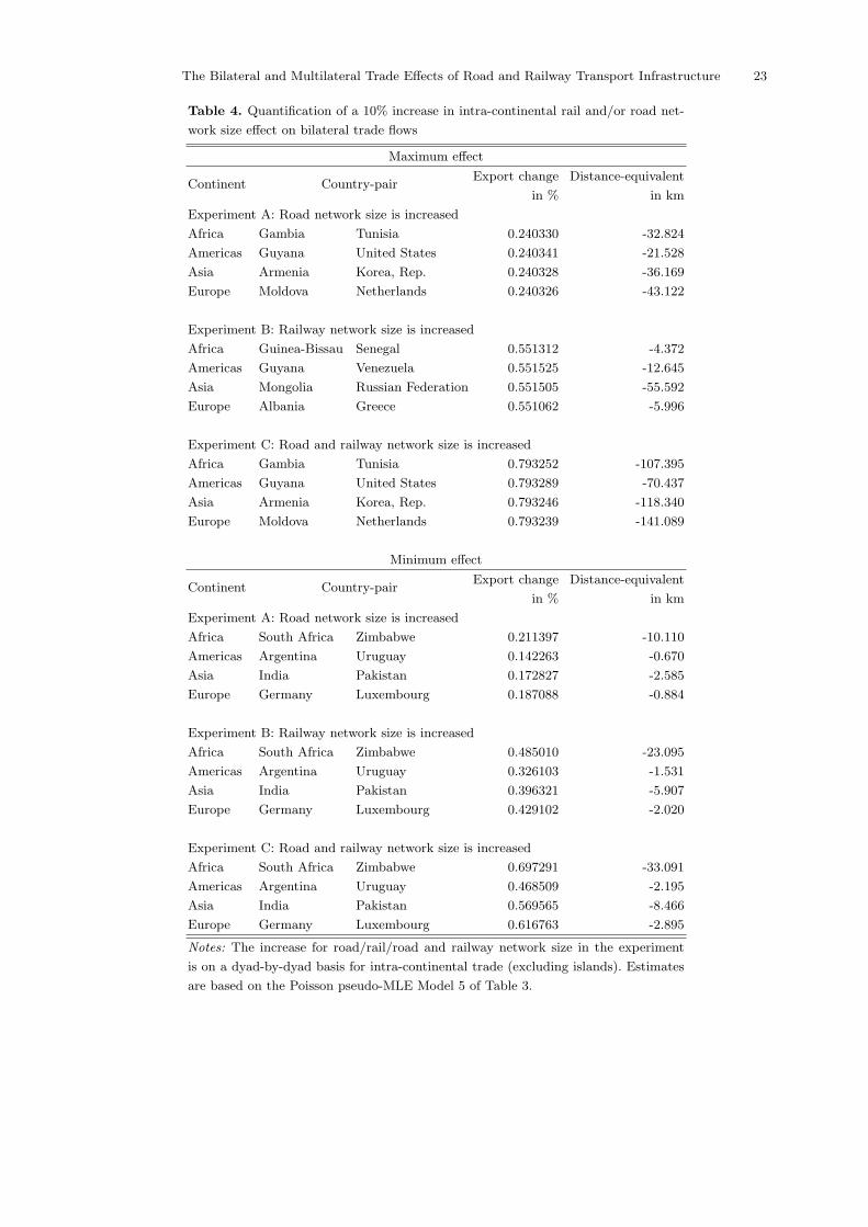
Table 4 summarizes the results regarding the range of export effects associated with dyad-

specific increases in rail and/or road networks by ten percent. The following insights can

be gained from this analysis. First, the maximum effects are very similar across continents,

irrespective of whether we change railway and road networks jointly or separately. This

indicates that the maximum change is hardly influenced by the indirect effects captured

by the multilateral resistance terms. To see this, compare the change reported in the bloc

of results on the top of Table 4 to the corresponding coefficients in Table 3 (multiplying

them by ten). Second, the minimum effects vary a lot more across continents than the

maximum ones. Hence, there are non-linearities brought about by multilateral resistance

which lead to a relatively large spread of ’marginal’ effects on some of the continents.11

In particular, the corresponding spread is large in the Americas, in Asia, and in Europe

(see the difference between the maximum and the minimum effects on these continents).

10 They use alternative values of σ, suggesting ones between 3 and 10. However, it turns out that the estimated

trade friction effects are fairly insensitive to the choice of σ in that range.11 Bougheas, Demetriades, and Morgenroth (2000) estimate output (GDP per capita growth) effects of infrastruc-

ture investments by means of extreme bounds analysis. They identify a fairly large variance in the elasticity

across countries, which is consistent with the variance of the effect of infrastructure we identify by means of

structural model estimation.


Third, a ten-percent change in railway networks leads to about twice as big of a change

in bilateral exports as a similar change of the road network.12 Fourth, the joint increase

in rail and road networks causes an effect which is about as large as the sum of the

independent changes.

− Table 4 −

Furthermore, the table provides information about the maximum and minimum distance-

equivalent of the ten-percent expansion in transport infrastructure network sizes. The

distance-equivalent effect (DE) in percent can be approximated by13

DE = 100 ∗

{exp

[ln

(∆Xij

100+ 1

)1

βDIST

]− 1

}, (6)

where Xij are the estimated infrastructure-induced trade effects as reported in Table 4,

and βDIST is the estimated distance coefficient, corresponding to −0.456. With the cor-

responding bilateral distance at hand, we may then compute the distance-equivalent of

a ten-percent increase in bilateral transport infrastructure networks. The distance coef-

ficient is negative and the estimated dyad-specific trade effects are positive throughout.

Accordingly, the ten-percent increase in transport infrastructure is equivalent to a reduc-

tion in bilateral distance for these country-pairs. For a joint increase in rail and road

networks, the trade effects correspond to a reduction in bilateral distance in the range

of about 2 kilometers (in the Americas: between Argentina and Uruguay) and about 141

kilometers (in Europe: between Moldova and the Netherlands).

12 With this, it is interesting to recall that the railway network size is much smaller on average than the road

network size, according to Table 2.13 This corresponds to direct distance effects only, ignoring any feedback through multilateral resistance. Account-

ing for the latter would preclude any analytical treatment of this issue.


In Table 5, we compute the impact of a ten-percent change in transport network in-

frastructure (roads, railways, roads and railways) for all intra-continental dyads on intra-

continental trade.14

− Table 5 −

These intra-continental trade effects are based on two sources: direct effects associated

with average dyad-specific changes in road and/or railway network size – i.e., the effect

in the nominator of (1) – and indirect effects brought about by changes in the average

multilateral resistance terms due to changes in transport infrastructure network size in

this and other dyads. The trade effects may be summarized as follows.

A simultaneous expansion of transport network size across dyads triggers trade effects of

less than one percent per dyad throughout. While a larger railway network raises intra-

continental trade for all continents except Europe, a larger road network may lead to

negative indirect (multilateral resistance) effects which outweigh the positive direct ones

for all continents except Africa. This indicates that a joint increase in transport infrastruc-

ture networks offsets the direct positive effects identified in Table 4, which supports Bond’s

(2006) hypothesis about the potential detrimental effects of transport infrastructure on

other countries through the terms of trade. Note again that the elasticity of bilateral ex-

ports with respect to joint road network size is about 0.025 according to Table 3. Hence,

a ten-percent increase in road network size should raise bilateral exports by about 0.25

percent. This direct effect is more than offset in the Americas, Asia, and Europe by the

negative indirect effects induced by multilateral trade resistance there. Even a joint in-

crease in road and railway network size leads to a decline in intra-continental trade of

Europe.

14 Whether we expand the network size only at one continent at a time or at all continents simultaneously does not

change the effects on intra-continental trade. However, the trade diverting effects for other continents are much

smaller if we change the network size at one continent at a time only. We know this from a set of experiments

which we suppress here for the sake of brevity.


Since the changes in transport infrastructure network size induce trade effects that are

smaller due to multilateral trade resistance than the dyad-specific ones in Table 4, also

the distance-equivalents are. For instance, intra-continental trade in the Americas rises by

0.003 percent if both road and railway infrastructure increase by ten percent. The distance-

equivalent effect in percent of an increase in transport network size in the Americas is then

100{exp

[ln(

0.026100

+ 1)

1−0.456

]− 1}

≃ −0.008%. Given that the average bilateral intra-

continental distance in the Americas is about 3, 067 kilometers, the distance equivalent to

a ten-percent increase in road and railway network size amounts to less than 0.3 kilometers

for the average country-pair on that continent. This is less than the minimum effect of a

dyad-specific change on that continent, and about 300 times smaller than the maximum

dyad-specific change on that continent, according to Table 4. A similar relative increase

of road and railway networks in Africa (Asia) would be equivalent to a reduction in

average bilateral distance on the continent by about 24 (1.4) kilometers. A ten-percent

increase in Europe’s intra-continental transport network leads to less international (and

more intra-national) trade, there. However, the distance-equivalent of this effect is about

4 kilometers.

Overall, the second experiment provides strong support for Eric Bond’s (2006) hypothesis

that uncoordinated transport infrastructure investments may exert detrimental conse-

quences on trade and welfare abroad through spillover effects on other countries’ terms of

trade. The latter supports arguments in favor of infrastructure policy coordination, since

”[i]nfrastructure agreements can be used to internalize these effects, leading to an efficient

choice of infrastructure” (see Bond, 2006, p. 485).

6 Conclusions

This paper analyzes the role of railway versus road transport infrastructure network size

for bilateral trade flows in the world economy. The empirical model integrates two impor-


tant features: that country-pairs depend on each other through their impact on their own

and others’ terms of trade; and that many of the possible bilateral trade flows are zero.

This brings about two sources of non-linearity: one related to the impact of dyad-specific

trade frictions (in our case, their relaxation through transport infrastructure) through

their impact on aggregate income on other countries’ consumer prices; and a second one

through the requirement of non-(log-)linear model estimation to respect numerous zeros

in the world trade flow matrix.

The non-linear modeling leads to heterogeneous effects of the considered (land) transport

infrastructure networks at the level of both country-pairs and continents. We undertake

two experiments to answer a set of questions that should be interesting to policy makers.

First, we change railway and/or road network size for each dyad. This allows us to answer

two questions: How big is the impact of railway versus road networks on international

trade, given that a a single country-pair changes its network size? For which countries’

international trade does a homogeneous increase of ten percent in network size produce

the largest versus the smallest effects? There, it turns out that a ten percent expansion

of railway networks is about twice as ’productive’ for international trade as one of road

networks across all continents. However, trade responds by less than a percent to such a

change. Country-pairs in the Americas are among the least responsive ones to changes in

railway and road transport network sizes.

Furthermore, we compute the corresponding trade effects if such a change occurs simul-

taneously for the other country-pairs on a continent. It turns out that this is harmful

from the average country-pair’s perspective on a continent. The simultaneous expansion

of other countries’ infrastructure networks partly (and on some continents more than

fully) offsets the positive direct effects on bilateral trade. In particular, this is the case

for road infrastructure networks. We conclude that this does not mean that countries are

better off by not investing in transport infrastructure if others do. By way of contrast,


the general trend in infrastructure network expansion abroad creates strong incentives for

individual countries to invest in their networks. Otherwise, they would suffer the negative

effects associated with the redirection of trade through the transport infrastructure net-

work expansion abroad. However, the negative spillover effects to other economies suggest

that infrastructure policy coordination should be particularly important to minimize the

possible detrimental cross-border effects of uncoordinated investments. Overall, we find

that – given the existence of road and railway networks – small to moderate changes in

today’s infrastructure networks are expected to exert tiny effects on trade flows, GDP,

and welfare.

A Country coverage (180 economies)

Afghanistan, Albania, Algeria, Angola, Antigua and Barbuda, Argentina, Armenia,

Aruba, Australia, Austria, Azerbaijan, Bahamas, Bahrain, Bangladesh, Barbados, Be-

larus, Belgium, Belize, Benin, Bermuda, Bolivia, Bosnia and Herzegovina, Brazil, Brunei,

Bulgaria, Burkina Faso, Burundi, Cambodia, Cameroon, Canada, Cape Verde, Central

African Republic, Chad, Chile, China, Colombia, Comoros, Congo (Dem. Rep.), Congo

(Rep.), Costa Rica, Cote d’Ivoire, Croatia, Cyprus, Czech Republic, Denmark, Djibouti,

Dominica, Dominican Republic, Ecuador, Egypt, El Salvador, Equatorial Guinea, Esto-

nia, Ethiopia, Fiji, Finland, France, French Polynesia, Gabon, Gambia, Georgia, Germany,

Ghana, Greece, Greenland, Grenada, Guatemala, Guinea, Guinea-Bissau, Guyana, Haiti,

Honduras, Hong Kong, Hungary, Iceland, India, Indonesia, Iran, Iraq, Ireland, Israel, Italy,

Jamaica, Japan, Jordan, Kazakhstan, Kenya, Kiribati, Korea (Rep.), Kuwait, Kyrgyz

Republic, Lao PDR, Latvia, Lebanon, Libya, Lithuania, Luxembourg, Macao, Macedo-

nia (FYR), Madagascar, Malawi, Malaysia, Maldives, Mali, Malta, Mauritania, Mauri-

tius, Mexico, Moldova, Mongolia, Morocco, Mozambique, Myanmar, Nepal, Netherlands,

Netherlands Antilles, New Caledonia, New Zealand, Nicaragua, Niger, Nigeria, Norway,


Oman, Pakistan, Panama, Papua New Guinea, Paraguay, Peru, Philippines, Poland, Por-

tugal, Qatar, Romania, Russian Federation, Rwanda, Samoa, Sao Tome and Principe,

Saudi Arabia, Senegal, Serbia and Montenegro, Seychelles, Sierra Leone, Singapore, Slo-

vak Republic, Slovenia, Solomon Islands, Somalia, South Africa, Spain, Sri Lanka, St. Kitts

and Nevis, St. Lucia, Vincent and the Grenadines, Sudan, Suriname, Sweden, Switzerland,

Syrian Arab Republic, Tajikistan, Tanzania, Thailand, Togo, Tonga, Trinidad and Tobago,

Tunisia, Turkey, Turkmenistan, Uganda, Ukraine, United Arab Emirates, United King-

dom, United States, Uruguay, Uzbekistan, Vanuatu, Venezuela (RB), Vietnam, Yemen

(Rep.), Zambia, Zimbabwe.

B Gaussian, Gamma, and negative binomial PMLE

In Table A1, we summarize the results from three alternative generalized linear models:

one based on Gaussian PMLE, another one based on Gamma PMLE, and a third one

based on negative binomial PMLE. Assuming normally distributed residuals, Gaussian

PMLE corresponds to OLS of bilateral exports in levels on the right-hand-side variables

in logs. Gamma PMLE is suited for data with non-negative values.

− Table A1 −

According to the pseudo R2s, none of the models summarized in Table A1 is preferred

against the Poisson PMLE for the data at hand. See also Santos Silva and Tenreyro (2006)

for a smorgasbord of advantages of Poisson PMLE over other models.

References

Anderson, James E. and Eric van Wincoop (2003), Gravity with gravitas: A solution to

the border puzzle, American Economic Review 93, 170-192.


Bond, Eric W. (1997), Transportation infrastructure investments and regional trade lib-

eralization, Working Paper no. WPS 1851, The World Bank (a revised version of the

paper has been published under the same title in 2006; see below).

Bond, Eric W. (2006), Transportation infrastructure investments and trade liberalization,

Japanese Economic Review 57, 483-500.

Bougheas, Spiros, Panicos O. Demetriades, and Edgar L.W. Morgenroth (1999), In-

frastructure, transport costs and trade, Journal of International Economics 47, 169-

189.

Bougheas, Spiros, Panicos O. Demetriades, and Edgar L.W. Morgenroth (2000), In-

frastructure, specialization, and economic growth, Canadian Journal of Economics

33, 506-522.

Cameron, Colin A. and Pravin K. Trivedi (1998), Regression Analysis for Count Data,

Econometric Society Monograph No. 30, University Press, Cambridge, UK.

Cameron, Colin A. and Pravin K. Trivedi (2005), Microeconometrics: Methods and Ap-

plications, Cambridge University Press, New York, NY.

Francois, Joseph and Miriam Manchin (2007), Institutions, infrastructure, and trade,

Policy Research Working Paper no. WPS 4152, The World Bank.

Fujimura, Manabu and Christopher Edmonds (2006), Impact of cross-border transport

infrastructure on trade and investment in the GMS, Discussion Paper no. 48, Asian

Development Bank.

Greene, William H. (2003), Econometric Analysis, 5th edition, Prentice Hall, New Jersey.

Limao, Nuno and Anthony J. Venables (2001), Infrastructure, geographical disadvantage,

transport costs and trade, World Bank Economic Review 15, 451-479.


Manning, Willard G. and John Mullahy (2001), Estimating log models: to transform or

not to transform?, Journal of Health Economics 20, 461-494.

McCullagh, Peter and John A. Nelder (1989), Generalized Linear Models, 2ed edition,

Chapman and Hall, London.

Nordas, Hildegunn K. and Roberta Piermartini (2004), Infrastructure and trade, Eco-

nomic Research and Statistics Division Staff Working Paper no. 2004-04, World Trade

Organization.

Santos Silva, Joao M.C. and Silvana Tenreyro (2006), The log of gravity, Review of

Economics and Statistics, 88, 641-658.

Wilson, John S., Catherine L. Mann, and Tsunehiro Otsuki (2004), Assessing the poten-

tial benefit of trade facilitation: A global perspective, Policy Research Working Paper

no. 3224, The World Bank.

Winkelmann, Rainer (2003), Econometric Analysis of Count Data, 4th edition, Springer

Verlag, Berlin.

Wooldridge, Jeffrey M. (2002), Econometric Analysis of Cross Section and Panel Data,

MIT Press, Cambridge, Massachusetts.


Table 1. Descriptive statistics A

Variable Mean Std. dev.

Bilateral exports 143.90 1970.08

Exporter (importer) road network size (km) 151312.50 548823.10

Exporter (importer) railway network size (km) 6296.01 20512.78

Exporter (importer) number of airports 249.07 1167.54

Exporter (importer) number of ports 10.04 21.25

Exporter (importer) GDP 165248.50 715643.10

Exporter-to-importer bilateral distance 7906.94 4541.45

Exporter/importer common official language indicator 0.15 0.35

Exporter/importer common colonial relationship indicator 0.01 0.11

Exporter/importer recent colonial relationship indicator 0.01 0.08

Exporter/importer same country indicator 0.01 0.09

Exporter/importer both landlocked indicator 0.03 0.17

Exporter/importer regional trade agreement indicator 0.08 0.28

Notes: All variables are in levels rather than logs. There are 32,220 observations. Road and

railway network size are measured in kilometres (km).

Table 2. Descriptive statistics B

Continent Railways Roads

Africa 1685.15 39080.31

America (North and South) 9953.45 286307.61

Asia 7440.73 168346.84

Europe 7398.82 151373.36

Oceania 4769.36 94602.36

Average 6296.01 151312.50

Notes: There are 7,140 intra-continental relationships.

The

Bila

teraland

Multila

teralTra

de

Effects

ofR

oad

and

Railw

ayTra

nsp

ort

Infra

structu

re22

Table 3. Regression results for Anderson and van Wincoop-type models with and without infrastructure variables

Log-linear Poisson pseudo-MLE

Model 1 Model 2 Model 3 Model 4 Model 5 Model 6

Log exporter plus importer - -0.022 -0.023 - 0.025 0.025

road network size - (0.004) (0.004) - (0.006) (0.006)

Log exporter plus importer - 0.061 0.062 - 0.058 0.057

railway network size - (0.011) (0.011) - (0.007) (0.050)

Exporter plus importer - - 1.045 - - 1.319

number of airports - - (0.052) - - (0.050)

Exporter plus importer - - 2.849 - - 6.723

number of ports - - (0.908) - - (0.917)

Log exporter-to-importer -1.533 -1.601 -1.600 -0.670 -0.456 -0.453

bilateral distance (0.026) (0.036) (0.036) (0.032) (0.041) (0.041)

Exporter/importer common 0.455 0.466 0.466 0.481 0.360 0.344

official language indicator (0.059) (0.059) (0.059) (0.072) (0.066) (0.064)

Exporter/importer common 0.817 0.822 0.822 -0.215 0.016 0.030

colonial relationship indicator (0.079) (0.079) (0.079) (0.181) (0.150) (0.149)

Exporter/importer recent 1.865 1.793 1.789 0.458 0.469 0.480

colonial relationship indicator (0.130) (0.131) (0.131) (0.201) (0.184) (0.182)

Exporter/importer same 0.810 0.584 0.570 0.874 0.710 0.700

country indicator (0.153) (0.158) (0.158) (0.227) (0.172) (0.173)

Exporter/importer both 0.771 0.740 0.657 0.371 0.495 0.127

landlocked indicator (0.126) (0.126) (0.130) (0.216) (0.189) (0.188)

Exporter/importer regional 0.477 0.486 0.486 0.681 0.477 0.490

trade agreement indicator (0.057) (0.057) (0.057) (0.075) (0.080) (0.079)

Dependent variable ln Xij ln Xij ln Xij Xij Xij Xij

Observations 15,366 15,366 15,366 32,220 32,220 32,220

Countries 180 180 180 180 180 180

R2 and pseudo R2 0.719 0.720 0.720 0.947 0.950 0.951

Log pseudo-likelihood - - - -980,866 -912,105 -902,637

Log pseudo-likelihood constant only - - - -18,342,021 -18,342,021 -18,342,021

Notes: Fixed country effects are not reported. The standard errors are given in parentheses and are based

on Eicker-White corrections of the variance-covariance matrix.


Table 4. Quantification of a 10% increase in intra-continental rail and/or road net-

work size effect on bilateral trade flows

Maximum effect

Export change Distance-equivalentContinent Country-pair

in % in km

Experiment A: Road network size is increased

Africa Gambia Tunisia 0.240330 -32.824

Americas Guyana United States 0.240341 -21.528

Asia Armenia Korea, Rep. 0.240328 -36.169

Europe Moldova Netherlands 0.240326 -43.122

Experiment B: Railway network size is increased

Africa Guinea-Bissau Senegal 0.551312 -4.372

Americas Guyana Venezuela 0.551525 -12.645

Asia Mongolia Russian Federation 0.551505 -55.592

Europe Albania Greece 0.551062 -5.996

Experiment C: Road and railway network size is increased

Africa Gambia Tunisia 0.793252 -107.395

Americas Guyana United States 0.793289 -70.437

Asia Armenia Korea, Rep. 0.793246 -118.340

Europe Moldova Netherlands 0.793239 -141.089

Minimum effect

Export change Distance-equivalentContinent Country-pair

in % in km

Experiment A: Road network size is increased

Africa South Africa Zimbabwe 0.211397 -10.110

Americas Argentina Uruguay 0.142263 -0.670

Asia India Pakistan 0.172827 -2.585

Europe Germany Luxembourg 0.187088 -0.884

Experiment B: Railway network size is increased





Experiment C: Road and railway network size is increased





Notes: The increase for road/rail/road and railway network size in the experiment

is on a dyad-by-dyad basis for intra-continental trade (excluding islands). Estimates

are based on the Poisson pseudo-MLE Model 5 of Table 3.


Table 5. Quantification of the intra-continental trade effect of a 10% increase in intra-

continental rail and/or road network size

Africa Americas Asia Europe

Roads

Total effect on intra-continental trade 0.158 -0.073 -0.044 -0.111

Intra-continental distance-equivalent effect in km -12.312 4.942 3.810 3.456

Railways

Total effect on intra-continental trade 0.143 0.077 0.060 -0.026

Intra-continental distance-equivalent effect in km -11.139 -5.170 -5.158 0.814

Roads and Railways

Total effect on intra-continental trade 0.301 0.003 0.016 -0.137

Intra-continental distance-equivalent effect in km -23.402 -0.232 -1.337 4.271

Average bilateral intra-continental distance in km 3553.32 3067.00 3914.43 1417.36

Notes: Estimates are based on the Poisson pseudo-MLE Model 5 of Table 3.

The

Bila

teraland

Multila

teralTra

de

Effects

ofR

oad

and

Railw

ayTra

nsp

ort

Infra

structu

re25

Table A1. Regression results for Gaussian, Gamma, and Negative binomial PMLE models

Gaussian pseudo-MLE Gamma pseudo-MLE Negative binomial

pseudo-MLE

Model 7 Model 8 Model 9 Model 10 Model 11 Model 12

Log exporter plus importer road network size - 4.573 - -0.0002 - 0.0189

- (3.502) - (0.000) - (0.004)

Log exporter plus importer railway network size - 290.753 - 0.0000 - 0.0972

- (75.937) - (0.000) - (0.012)

Exporter plus importer number of airports - 121.189 - -0.0095 - 1.5810

- (98.505) - (0.001) - (0.047)

Exporter plus importer number of ports - 15781.750 - 0.0060 - 2.9302

- (2633.071) - (0.004) - (0.803)

Log exporter-to-importer bilateral distance -226.851 -72.386 0.0003 0.0002 -1.5239 -1.5384

(39.991) (31.910) (0.000) (0.000) (0.025) (0.033)

Exporter/importer common official language indicator -5.389 -40.985 -0.0003 -0.0008 0.4345 0.4315

(40.937) (39.692) (0.000) (0.001) (0.056) (0.054)

Exporter/importer common colonial relationship indicator 10.908 29.905 0.0002 -0.0022 0.8138 0.8292

(35.211) (35.042) (0.000) (0.001) (0.069) (0.069)

Exporter/importer recent colonial relationship indicator -350.195 -507.916 -0.0006 -0.0030 1.9967 1.9659

(229.997) (236.179) (0.000) (0.004) (0.134) (0.134)

Exporter/importer same country indicator -143.761 -894.920 0.0001 -0.0009 1.1738 0.9194

(297.956) (388.265) (0.001) (0.005) (0.142) (0.145)

Exporter/importer both landlocked indicator 43.827 -262.813 -0.0017 -0.0052 0.8206 0.7504

(20.422) (56.198) (0.000) (0.002) (0.119) (0.122)

Exporter/importer regional trade agreement indicator 578.088 437.590 0.0000 -0.0004 0.4176 0.4030

(106.922) (76.925) (0.000) (0.000) (0.054) (0.053)

Observations 32,220 32,220 32,220 32,220 32,220 32,220

Countries 180 180 180 180 180 180

Pseudo R2 0.006 0.008 0.000 0.000 0.689 0.690

Log pseudo-likelihood -288,308 -287,898 -1.62E+14 -1.69E+14 -59,831 -59,664

Log pseudo-likelihood constant only -290,133 -290,133 -1.62E+14 -1.69E+14 -192,438 -192,438

Notes: In all models, the dependent variable is Xij . Fixed country effects are not reported. The stanard errors reported in parantheses

are based on Eicker-White corrections of the variance-covariance matrix.

the bilateral and multilateral trade eﬀects of road … · even an increase of the joint railway...

Documents