THE BILATERAL J-CURVE OF TURKEY FOR CONSUMPTION, CAPITAL

AND INTERMEDIATE GOODS

A THESIS SUBMITTED TO

THE GRADUATE SCHOOL OF SOCIAL SCIENCES

OF

MIDDLE EAST TECHNICAL UNIVERSITY

BY

GĠZEM KESKĠN

IN PARTIAL FULFILLMENT OF THE REQUIREMENTS

FOR

THE DEGREE OF MASTER OF SCIENCE

IN

THE DEPARTMENT OF ECONOMICS

JULY 2008

Approval of the Graduate School of Social Sciences

Prof. Dr. Sencer Ayata

Director

I certify that this thesis satisfies all the requirements as a thesis for the degree of

Master of Science.

Prof. Dr. Haluk Erlat

Head of the Department

This is to certify that we have read this thesis and that in our opinion it is fully

adequate, in scope and quality, as a thesis for the degree of Master of Science.

Assoc. Prof. Dr. Elif Akbostancı

Supervisor

Examining Committee Members:

Prof. Dr. Erdal Özmen (METU, ECON) __________________

Assoc. Prof. Dr. Elif Akbostancı (METU, ECON) __________________

Assoc. Prof. Dr. Uğur Soytaş (METU, BA) __________________

iii

I hereby declare that all information in this document has been obtained and

presented in accordance with academic rules and ethical conduct. I also

declare that, as required by these rules and conduct, I have fully cited and

referenced all material and results that are not original to this work.

Name, Last Name: Gizem KESKİN

Signature :

iv

ABSTRACT

THE BILATERAL J-CURVE OF TURKEY FOR CONSUMPTION, CAPITAL

AND INTERMEDIATE GOODS

Keskin, Gizem

MS., Department of Economics

Supervisor: Assoc. Prof. Dr. Elif Akbostancı

June 2008, 69 pages

This study analyzes the J-curve effect for Turkey‟s bilateral trade with her three

main trading partners; Germany, USA and Italy, for consumption, capital and

intermediate goods. The bounds test is used to test for cointegration among the

trade balance, the real bilateral exchange rate, the real domestic income and the

real foreign income. The results show that the real exchange rate is not a

significant determinant of trade in the short run. In the long run, it is significant

only for trade with USA in consumption goods. Moreover, J-curve does not exist

for Turkey‟s bilateral trade with Germany, USA, and Italy in consumption, capital

and intermediate goods. The results support existence of a link between the

bilateral trade balances and the real domestic income both in the short run and the

long run.

Keywords: J-curve, Bounds test approach, Bilateral trade, BEC definition,Turkey

v

ÖZ

TÜRKĠYENĠN TÜKETĠM, YATIRIM VE ARAMALI TĠCARET

DENGESĠNDE ĠKĠ TARAFLI J-EĞRĠSĠ ETKĠSĠ

Keskin, Gizem

Yüksek Lisans, Ġktisat Bölümü

Tez Yöneticisi: Doç. Dr. Elif Akbostancı

Temmuz 2008, 69 sayfa

Bu çalışma Türkiye‟nin Almanya, A.B.D. ve Ġtalya ile ikitaraflı tüketim, yatırım

ve aramalı ticaretindeki J-eğrisi etkisini incelemektedir. Ticaret dengesi, reel

döviz kuru, yurtiçi reel gelir ve yabancı reel gelir arasındaki eşbütünleşme sınır

testi yöntemiyle incelenmiştir. Sonuçlar döviz kurunun kısa dönemde ticaretin

belirleyicilerinden biri olmadığını göstermektedir. Uzun dönemde ise döviz kuru

yalnızca A.B.D. ile tüketim malları ticaretinde etkilidir. Ayrıca Türkiye‟nin

Almanya, A.B.D. ve Ġtalya ile ikitaraflı tüketim, yatırım ve aramalı ticaretinde J-

eğrisi etkisi bulunmamaktadır. Sonuçlar hem kısa dönemde, hem de uzun

dönemde ikitaraflı ticaret dengesi ve yurtiçi reel gelir arasında bir ilişki olduğunu

desteklemektedir.

Anahtar Sözcükler: J-eğrisi, Sınır testi yaklaşımı, Ġkitaraflı ticaret, BEC tanımı,

Türkiye

vi

To my family

vii

ACKNOWLEDGMENTS

I want to thank my thesis supervisor, Assoc. Prof. Dr. Elif Akbostancı, for her

close supervision, contributions, and academic support throughout this study. I am

especially grateful to her because this study would not have been completed

without her encouragement and motivation. I am grateful to the examining

committee members, Prof. Dr. Erdal Özmen and Assoc. Prof. Dr. Uğur Soytaş, for

their precious contributions and criticisms; to Assist. Prof. Dr. Engin Küçükkaya

for his careful review and valuable suggestions, and to Assoc. Prof. Dr. Ramazan

Sarı for his guidance for coping with the econometric technique used in this study.

I would like to thank the Scientific and Technological Research Council of

Turkey (TÜBĠTAK) for their scholarship.

I thank my colleagues from department of Business Administration; Ufuk Kara,

especially for his academic and technical support, Ayça Güler-Edwards and

Mesrur Börü for their friendship, patience, and encouragement; and my friends

from department of Economics; Nutiye Seçkin, for her friendship, motivation and

moral support, and Eda Gülşen for her technical help throughout this study.

I express my deepest gratitude to my parents, Nurten and Ali Osman Keskin, for

teaching me everything that makes me who I am today. I am indebted to my

sister, Sinem Keskin, for being my best friend and being by my side anytime and

anywhere. I am sure that nothing will change in the future. Last of all, I want to

thank my aunt, Gülten Pamir, for her caring attitude and constant support

throughout my life.

viii

TABLE OF CONTENTS

PLAGIARISM ....................................................................................................... iii

ABSTRACT ........................................................................................................... iv

ÖZ............................................................................................................................ v

ACKNOWLEDGMENTS ..................................................................................... vii

TABLE OF CONTENTS ..................................................................................... viii

LIST OF TABLES .................................................................................................. x

LIST OF FIGURES ................................................................................................ xi

CHAPTER

1.INTRODUCTION: THE J-CURVE .................................................................... 1

2.LITERATURE REVIEW: THEORY AND EVIDENCE .................................... 5

2.1. A Theoretical Background ............................................................................ 5

2.2. Empirical Studies .......................................................................................... 9

2.2.1. Studies at Aggregate Level .................................................................... 11

2.2.1.1. Multi-Country Studies ..................................................................... 11

2.2.1.2 Single Country Studies: .................................................................... 13

2.2.2. Studies at Bilateral Level ....................................................................... 15

ix

2.2.3 Studies at Industry or Product Level ...................................................... 17

2.2.4. Emprical Findings for Turkey: .............................................................. 19

3.THE MODEL AND THE DATA ...................................................................... 22

3.1. Introduction of the Model and the Data Sources ......................................... 22

3.2. A General Look into the Raw Data ............................................................. 26

3.3. Unit Root Tests ............................................................................................ 39

4.THE EMPRICAL ANALYSIS .......................................................................... 43

5. CONCLUSIONS ............................................................................................... 57

REFERENCES ...................................................................................................... 63

APPENDICES

APPENDIX A: Abbreviations Used for Variables ............................................... 67

APPENDIX B: Shares of Trade Volumes for Each Trading Partner .................... 64

APPENDIX C: Lag Lengths Suggested By Information Criteria ........................ 69

x

LIST OF TABLES

Table 3.1: ADF test results for levels of variables for USA...……………...……40

Table 3.2: ADF test results for first differences of variables for USA...…...……41

Table 3.3: ADF test results for levels of variables for Germany…………...……41

Table 3.4: ADF test results for first differences of variables for Germany…...…41

Table 3.5: ADF test results for levels of variables for Italy………………...……42

Table 3.6 : ADF test results for first differences of variables for Italy…...……...42

Table 4.1: The calculated F-statistics relevant for bounds test for different

lag lengths of the first differenced variables………….……………….….…47

Table 4.2: Summary of the results of the bounds test for cointegration……...….48

Table 4.3: The results of the bounds test for different dependent variables……..49

Table 4.4: The long run estimates of the relationship between the levels…….....50

Table 4.5: Estimated short run coefficients of the variables ………………….…54

Table 4.5 (cont‟d): Estimated short run coefficients of the variables …………...55

Table A.1: Lag lengths suggested by AIC and SC based on an unrestricted

VAR model…………………………………………..……………………...64

xi

LIST OF FIGURES

Figure 3.1: Trade balance with USA in consumption goods (ltbcon_usa) and

real exchange rate between YTL and USD (lrer)…..……………..………....27

Figure 3.2: Trade balance with USA in capital goods (ltbcap_usa) and

real exchange rate between YTL and USD (lrerp) .........................................28

Figure 3.3: Trade balance with USA in intermediate goods (ltbint_usa) and

real exchange rate between YTL and USD (lrerp)……….………….........…28

Figure 3.4: Trade balance with USA in consumption, capital and

intermediate goods ………………….......................…………….…..…...…29

Figure 3.5: Trade balance with Germany in consumption goods (ltbcon_germ)

and the real exchange rate between YTL and DM (lrer)……........…………31

Figure 3.6: Trade balance with Germany in capital goods (ltbcap_germ)

and the real exchange rate between YTL and DM (lrerp)……….…...……...32

Figure 3.7: Trade balance with Germany in intermediate goods (ltbint_germ)

and the real exchange rate between YTL and DM (lrerp)…..........................32

Figure 3.8: Trade balance with Germany in consumption, capital and

intermediate goods…….............................................................................….33

Figure 3.9: Trade balance with Italy in consumption goods (ltbcon_ital) and

the real exchange rate between YTL and ITL (lrer)……...………......……..33

xii

Figure 3.10: Trade balance with Italy in capital goods (ltbcap_ital) and the

real exchange rate between YTL and ITL (lrerp)……….…...……….…......34

Figure 3.11: Trade balance with Italy in intermediate goods (ltbint_ital) and

the real exchange rate between YTL and ITL (lrerp)…………….………....35

Figure 3.12: Trade balance with Italy in consumption, capital and

intermediate goods………………………...……………………………..….36

Figure 3.13: Trade balance in consumption goods with USA, Italy

and Germany…………………………………..…………………………….37

Figure 3.14: Trade balance in capital goods with USA, Italy and Germany….....38

Figure 3.15: Trade balance in intermediate goods with USA, Germany and

Italy …………………..……………………………………………………..38

1

CHAPTER 1

INTRODUCTION: THE J-CURVE

The exchange rate is an easily observable variable giving clues about the current

state of a country‟s economy, as Mishkin (1999) states. Besides being a crucial

determinant of international competitiveness, Mishkin (1999) mentions its role as

a monetary policy tool for controlling inflation and maintaining stability of the

economy through exchange rate targeting, used for a long period of time.

However, increasing capital mobility around the world and developing financial

instruments to bypass existing capital controls, have made it difficult and painful

for the countries to maintain their control over the exchange rate. Consequently,

economies shift to floating rate regimes and accept other monetary policy

regimes, such as inflation targeting, to ensure price stability, and this is the case

for Turkey as well. Nevertheless, despite these developments, the exchange rate is

still a significant monetary variable. In fact, these trends have made the exchange

rate more volatile, more unpredictable and more prone to global shocks.

Moreover, as Domaç and Mendoza (2004) explain, even under inflation targeting

where the exchange rate needs to float, policymakers in emerging markets should

have an eye on its movements. Last of all, despite decreased control over the

exchange rates, belief in its significance for determining international

competitiveness is still widespread. The ongoing debate about insistence of Asian

countries to prevent their currencies from appreciating in order to protect their

export-led growth strategies is a strong evidence for belief in that linkage.

2

Undervalued currencies are seen as keys for success stories of trade surpluses

whereas overvalued ones are seen as the drivers for deficits. As a result, the

relationship between the trade balance and the exchange rate is worth examining.

In the broadest sense, the direction of the long run relationship between the

exchange rate (defined as home currency price of one unit of foreign currency)

and the trade balance is expected to be positive, assuming that Marshall-Lerner

condition holds. In other words, increases in exchange rate, that is deprecation of

domestic currency, is expected to make exports cheaper and imports more

expensive. As a result, the trade balance is anticipated to improve. Similarly,

appreciation of the domestic currency is expected to deteriorate the trade balance.

However, as first raised by Magee (1973), the adjustments may not be immediate.

As he mentions, the movement in the trade balance depends on the currency

denomination of the export and import contracts, on the extent of the pass-through

from the exchange rate to the prices of exports and imports, and on the volume

adjustments. As a result, he suggests that following devaluation, the trade balance

may continue to worsen in the short run before it starts to improve, evolving in a

J-like path, named as „J-curve effect‟. Therefore, devaluation used as a policy to

boost exports may result in an immediate adverse movement in the trade balance

instead. In the short run, this may conceal the long run positive effects of

devaluation (or depreciation) on the trade balance. Analysis of J-curve effect may

be helpful to prevent distorted judgments about the effect of weakening domestic

currency in the long run. Moreover, in order to take appropriate actions, whether

the deterioration is temporary resulting from a J-curve effect or permanent

resulting from other factors (such as low price elasticities, low product qualities,

or income related factors instead of price related ones) should be clarified. This

also underlines the importance of empirical investigation of the J-curve effect.

Shortly after the introduction of the J-curve concept by Magee (1973), researchers

tested whether the data for different countries and sample periods support the

3

theory empirically. Some of these empirical studies analyzed trade balance of a

country with all its trading partners aggregated together1. However, they were

criticized for suffering from aggregation problems, stated first by Rose and Yellen

(1989). This contribution led to a new trend of bilateral analysis in the literature2.

While bilateral analysis disaggregated the data with respect to the trading partners,

some disaggregated it with respect to the industry or to the product3.

The studies analyzing the Turkish J-curve, present mixed results about the long

run and short run relationship between the trade balance and the exchange rate4.

However, none of these studies presents evidence for J-curve effect. Except

Halıcıoğlu (2007), all the studies are carried at aggregate level. Therefore, this

study aims to analyze the J-curve for Turkey by clearing doubts about aggregation

bias mentioned by Rose and Yellen (1989) through disaggregating the trade

balance data with respect to two dimensions; the trading partner and the nature of

the product traded according to Broad Economic Categories (BEC) definition of

United Nations. The BEC definition groups the tradable goods into three main

categories according to their end use, consumption, capital and intermediate

goods. Examination of trade on these goods separately is expected to prevent

opposite movements of trade balances on these different types of goods from

offsetting each other. In addition, it aims to shed light on the different ways the

trade on each group responds to the movement in the exchange rate. Moreover,

the analysis is expected to differentiate the response of the production side of the

1 Miles (1979), Bahmani-Oskooee (1985), Felmingham (1988), Himarios (1989), Rose (1990),

Gupta-Kapoor and Ramakrishnan (1999), Narayan and Narayan (2004).

2 Rose and Yellen (1989), Wilson and Tat (2001), Bahmani-Oskooee and Goswami (2003),

Bahmani-Oskooee, Economidou, and Goswami (2006), Bahmani-Oskooee, Goswami, and

Talukdar (2008)

3 Carter and Pick (1989), Doroodian, Jung, and Boyd (1999), Bahmani-Oskooee and Ardalani

(2006), Baek (2006)

4 Rose (1990), Brada, Kutan, and Zhou (1997), Akbostancı (2004), Halıcıoğlu (2007), Bahmani-

Oskooee, Goswami, and Talukdar (2008)

4

economy from the demand side. The trade balance in capital and intermediate

goods are expected to follow the production side of the economy and the

economic growth closely. The trade balance in consumption goods is anticipated

to be affected more by demand side factors whereas the trade balances in capital

and intermediate goods are expected to be driven by supply side factors.

For analysis of bilateral J-curve on these goods, bounds testing approach of

Pesaran, Shin and Smith (2001) and ARDL approach of Pesaran and Shin (1999)

are used. Bounds testing is preferred for testing the existence of cointegration

among the variables, as it allows the variables to be stationary, integrated of order

one, or a combination of both. It is a simple joint significance test of the one

period lagged levels of the variables in the ARDL model. However, two sets of

nonstandard critical values are developed by Pesaran et al.. (2001) to compare the

calculated F-statistic for each significance level. If the calculated statistic exceeds

the upper bound critical value, the null hypothesis of no cointegration is rejected.

If, on the other hand, it falls below the lower bound, then no cointegration is not

rejected. The results are inconclusive if the calculated statistic lies between the

upper and the lower bounds. Following Pesaran et al. (2001), the analysis

continues with ARDL approach of Pesaran (1999) after the cointegration test. The

ARDL approach enables the examination of both the short run and the long run

dynamics, presenting all the information needed for complete J-curve analysis.

The rest of the study proceeds as follows: Chapter 2 presents a review of the

literature by both referring to the theoretical background and the empirical results

so far for different countries at different levels. Chapter 3 introduces the model,

presents the sources of the data and provides a general look into raw data

characteristics. Chapter 4 gives an explanation of the econometric technique used

and presents the empirical results. Chapter 5 provides a review of the findings and

restates important conclusions.

5

CHAPTER2

LITERATURE REVIEW: THEORY AND EVIDENCE

2.1. A Theoretical Background:

Before looking at the empirical findings about the relationship between the real

exchange rate and the trade balance, a reexamination of the underlying theory may

be useful. In most of the emprical studies, it is implicitly assumed that export

contracts are denominated in domestic currency whereas import contracts are

denominated in foreign currency. Moreover, the exchange rate pass-through to

export and import prices is assumed to be perfect. These implicit assumptions

provide some necessary underlying conditions for a J-curve to be observed. In

other words, unless some conditions are met, discussions of the J-curve concept

may be totally meaningles, or, no emprical evidence for J-curve may be a result of

failure to meet those prerequisites. For instance, as stated by Magee (1973),

Arndt and Dorrance (1987), and Carter and Pick (1989), if the trade balance is

calculated in foreign currency, and the export and import prices are also quoted in

foreign currency and are unaffected by depreciation, the trade balance figure will

not respond to any change in the real exchange rate for sure. As a result, in this

case, it would be meaningless to talk about the J-curve effect.

An analytical examination of the underlying conditions for a J-curve to be

observed is presented by Magee (1973). He explores the situations where an

6

exchange rate movement can or can not have an impact on the trade balance. He

mentions that even in the earlier periods of devaluation, when no quantity

adjustment takes place yet; the movement of the trade balance depends on the

currency denominations of contracts and the elasticities of import and export

demand and supply. Magee (1973) defines two different time periods before the

volume adjustments start: “the currency contract period” (p.305) and “the pass-

through period” (p.305).

“Currency contract period” refers to the time period when the devaluation occurs

but the contracts are already made and can not be changed. In other words, both

the quantity of the traded goods and the agreed on price (which may be in

domestic or foreign currency) stay the same. However, the value of the imports

and exports may be affected, depending on the currency denomination of exports,

imports and the trade balance. Analysis of “currency-contract period” (p.305) by

Magee (1973) reveals that the deterioration in the trade balance compared to the

pre-devaluation period may be possible if:

The trade balance is already in deficit and is expressed in terms of the

domestic currency while both export and import contracts are denomianted

in foreign currency.

The trade balance is already in surplus and is expressed in terms of the

foreign currency while both export and import contracts are denominated

in domestic currency.

Regardless of the type of currency denomination of the trade balance,

exports contracts are denominated in domestic currency while import

contracts are in foreign currency.

7

After the time period for already signed contracts has expired, in other words, the

currency contract period is over, the price adjustment sets in before quantities

adjust. Theoretically, the trade balance may move in any direction depending on

the changes in the price of the exports and the imports. In discussions of the J-

curve, it is implicitly assumed that the foreign currency price of imports stays the

same so that imports cost more domestic currency to the devaluing country. In the

same manner, the domestic currency price of the exports do not change so that

exports to the trade partners cost less in terms of that importing country‟s

currency. In other words, export prices are sticky in terms of the exporter

countries‟ currencies (Arndt and Dorrance 1987, Rose and Yellen 1989). As a

result, before volume effect comes in, decreased export revenue in foreign

currency and increased import expenditure in domestic currency will result in an

inevitable deterioration in the trade balance, denominated in any currency. This is

named as perfect pass-through.

However, Magee (1973) questions the perfect pass-through assumptions and

instead analyzes which way the trade balance may move depending on the

demand and supply elasticities of both exports and imports, for the period he

names as the “pass-through period”(p.305). He concludes that if there is perfect

pass-through on export and import side, then the trade balance is expected to

improve in the long run. However, before the volume adjustments, perfect pass-

through causes the trade balance to deteriorate in the short run, regardless of the

currency denomination.

According to Magee (1973), after the pass-through period, volume adjustments

take place depending on the elasticities of demand and supply. As a combination

of the “currency-contract period” (p.305), “pass-through period” (p.305) and the

quantity adjustments, final impact on the movement of the trade balance is

determined.

8

Junz and Rhomberg (1973) underline five types of lags to account for the late

response of the trade balance to fluctuations in the exchange rate. Recognition lag

exists because it takes some time for agents to recognize the change. Decision lag

refers to the time elapsing before agents make up their minds about new

purchases. Delivery lag is the gap between the ordering time and delivery time.

Replacement lag is the time that passes before new inventories become available.

Production lag is the time gap before producers realize the new market conditions

and shift resources accordingly.

Arndt and Dorrance (1987) bring a new theoretical perspective and claim that the

deterioration of the trade balance is important only if it causes a deficit in terms of

the foreign currency which should be financed by cutting domestic expenditure.

Since decrease in the domestic currency value of the trade balance does not signal

more foreign currency outflows, according to Arndt and Dorrance (1987), it

should be irrelevant to the discussion of the real effects of devaluation. So they

claim that the J-curve phenomenon should only be discussed whenever the trade

balance is denominated in foreign currency. Similar to “currency contract period”

(p.305) Magee (1973) mentions, they attribute existence of a J-curve mainly to the

stickiness in domestic currency prices of exports, causing export revenues to fall

in foreign currency. They also claim irrelevance of J-curve for small countries as

they are unable to affect foreign currency price of their tradables and accordingly

foreign currency value of their trade balance.

Wilson and Tat (2001) agree with Arndt and Dorrance (1987) on the irrelevance

of a J-curve discussion for small countries as they have no power in affecting

foreign currency price of their tradables. However, they also illustrate an

elasticities approach to show that J-curve may be observed even for small

countries with trade deficits that have low market power.

9

Turkey belongs to the category of „small countries‟ defined by Arndt and

Dorrance (1987) and Wilson and Tat (2001), because it does not invoice its

exports in domestic currency, as Berument and Dincer (2005) state.Instead,

exports are mostly denominated in Euros and imports are mostly denominated in

US dollars (USD). Therefore, the foreign currency value of the trade balance may

be unresponsive to the exchange rate movements. In order to neutralize the impact

of currency denomination of the trade balance in this study, following Brada et al.

(1997), the trade balance is made unit-free and defined as exports over imports.

Moreover, in this study, partial reduced form of the trade balance presented by

Rose and Yellen (1989) is used. As Doroodian, Jung, and Boyd (1999) state, this

model analyzes the movement in the trade balance directly and accounts for both

the pass-through and the quantity adjustment effects simultaneously.

2.2. Empirical Studies

The empirical findings regarding the significance of exchange rate movements in

determining trade balance vary across studies. A general conclusion is hard to

draw. Most of the studies use the partial reduced form of the trade balance,

presented by Rose and Yellen (1989)5. Instead of analyzing the export and import

demand functions seperately, Rose and Yellen (1989) solve those simultaneously

to end up with a model determining the trade balance. The model explains the

trade balance with the exchange rate, the domestic income and the foreign

income. Some studies modify the variables used. For instance, Felmingham

(1988) substitues the real exchange rate with the terms of trade. Gupta-Kapoor

and Ramakrishnan (1999) prefer to use nominal values of all the variables

asserting that J-curve is a totally nominal concept. Singh (2004) augments the

model with a variable representing the exchange rate volatility. Despite these

5 Rose (1990), Brada et al. (1997), Wilson and Tat (2001),Bahmani-Oskooee and Goswami

(2003), Akbostancı (2004), Narayan and Narayan (2004), Singh (2004), Bahmani-Oskooee et al.

(2006), Baek (2006), Halıcıoğlu (2007), Bahmani-Oskooee,Goswami and Talukdar (2008),

Bahmani-Oskooee and Kutan (2008)

10

minor differences, the majority of the literature on J-curve follows Rose and

Yellen (1989).

On the other hand, some studies aim to account for some factors Rose and Yellen

(1989) do not consider and thus use some additional variables. For instance, Miles

(1979) criticizes the previous studies for overlooking the effects of the fiscal and

monetary policy at the time of devaluation. To account for these effects, he

includes additional variables representing the monetary and fiscal policies of the

home country and the trading partners such as growth rates of the GDPs, domestic

portion of the high powered money and the government expenditures, all of which

are in nominal terms. Bahmani-Oskooee (1985) adds only the effect of money by

including domestic and foreign money variables. Himarios (1989) wants to

account for the monetary and fiscal policy effects altogether. Hence, he includes

domestic and foreign real government expenditures, domestic and foreign real

money balances, domestic and foreign interest rates in his model. Moreover, he

also accounts for the effects of anticipated devaluation.

Besides the models chosen, the nature of the analysis differs across studies. Early

studies analyze the trade balance at aggregate level, that is the trade with all

partners is summed together, proxies are used representing the weighted avarage

of the incomes of all those partners and effective exchange rate measures are

employed. However, empirical evidence fails to support the J-curve concept in

most of these studies. That failure is attributed to the problems brought about by

aggregate data (Rose and Yellen, 1989). The view that a J-like movement with

respect to one trading partner may be offset with an opposite movement with

respect to another country gains popularity. In order to overcome these problems,

later studies examine the trade balances at bilateral level. In some papers, the trade

balance is analyzed even at industry level or at product level. Next in this chapter,

a brief review of the results of all these studies at different levels are presented in

historical order.

11

2.2.1. Studies at Aggregate Level

2.2.1.1. Multi-Country Studies

Junz and Rhomberg (1973) examine manufactured goods‟ flows from 13

industrial countries. They find that the response of the flows of manufactured

goods to the changes in relative prices (including changes resulting from

fluctuations in exchange rates) is materialized in a period of four to five years

following the change. However, they do not observe a special path that the trade

balance follows.

Miles (1979) examines trade balance-devaluation relationship in 14 countries for

the period of 1956-1972. He accounts for effects of monetary and fiscal policies

on the movement of the trade balance. Consequently, he explains the change in

the trade balance with the difference between the income growth rates, difference

between the money supplies, difference between the government expenditures of

the home country and its trading partner as well as the exchange rate. All the

variables chosen are in nominal terms. Two methods are used, one is the residuals

test and the other is a direct test of the significance of the exchange rate in the

model. The results of the residuals test suggest that devaluation causes the trade

balance to deteriorate in 10 cases. Testing the significance of the exchange rate

directly, devaluation is found to improve the trade balance of France, Finland and

New Zealand and to deteriorate the trade balance of United Kingdom and Guyana.

The empirical findings do not even support a positive relationship between

exchange rate and the trade balance in majority of the cases, leaving aside the J-

curve effect.

Himarios (1989) explains the trade balance with a model including domestic and

foreign real incomes, domestic and foreign real government expenditures,

domestic and foreign real money balances, domestic and foreign interest rates,

expected devaluation and the real exchange rate. Data for two different sample

12

periods cover different sets of countries. For the period of 1953-1973, 15

countries are examined. The results support that for 80% of the cases, devaluation

causes an improvement in the trade balance while a J-pattern is observed only for

the UK. The other sample examines another set of 15 countries for the period of

1975-1984. Similarly, the results support a positive relationship between real

exchange rate and trade balance for 80% of the cases. Moreover, a J-curve pattern

is observed only for Ecuador, France, Greece and Zambia.

Rose (1990) analyzes the real trade balance at aggregate level for 30 countries

including Turkey. The real trade balance is explained with the real effective

exchange rate, the real domestic and foreign income. Annual data shows that only

for Tanzania and Thailand, the coefficients of the different lags of the real

exchange rate variable are jointly significant. Only for Thailand, devaluation is

found to improve the trade balance. Quarterly data supports joint significance of

the lagged exchange rate variables for six countries. However, in this case,

cumulative significant and positive effect of devaluation is not found in any of the

30 countries. Therefore, the exchange rate is concluded not to be a significant

variable in explaining the trade balance both in the long run and the short run.

Bahmani-Oskooee and Kutan (2008) try to explain the real trade balance with real

domestic income, real world income and the real effective exchange rate for 11

countries, which are a combination of new members and candidates of the

European Union.They find support for short run effect of the exchange rate on the

trade balance in 8 of the countries. The bounds testing results support

cointegration for some of the countries while the error correction model based

cointegration test support it for all of the 11 countries. Following J-curve

definition of Rose and Yellen (1989), stated as existence of negative short run

effect together with positive long run effect, Bahmani-Oskoee and Kutan (2008)

find evidence for J-curve effect in Bulgaria, Croatia and Russia.

13

2.2.1.2 Single Country Studies:

While the studies mentioned above concern a couple of countries, Felmingham

(1988) examines the J curve phenomenon for a single country, Australia. The

trade balance is explained by the terms of trade, expressed as a ratio of price of

exports to price of imports, domestic income and foreign income. The data is

examined in 3 different sample periods: 1965-1974 covers the period of fixed

exchange rate, 1974-1983 covers the period of managed floating and 1974-1985

includes years of free floating additionally. For the fixed exchange rate period,

weak evidence for J-curve is found and the improvement in the trade balance is

seen in 9 quarters. However, in the managed floating period, no evidence for J-

curve is found. Moreover, devaluation is not found to improve the trade balance in

the long run for this period. The Chow test reveals no structural change in the

third sample period, so the results for the managed floating period are valid for the

years of free floating as well. Felmigham (1988) concludes exchange rate not to

be a significant determinant of the trade balance. He attributes this

unresponsiveness of trade balance to devaluation, mainly to the low

substitutability of imports with domestic goods and with high competition from

third world exporters on Australian exports.

Gupta-Kapoor and Ramakrishnan (1999) examine Japanese quarterly data for the

period covering 1975-1996. The paper is differentiated from the rest of the

literature by claiming that the J-curve phenomenon is a nominal concept and by

examining the effects of appreciation rather than depreciation. They explain the

nominal trade balance with nominal effective exchange rate, nominal domestic

income and weighted average of the nominal incomes of Japan‟s main trading

partners. Gupta-Kapoor and Ramakrishnan (1999) find evidence supporting the

long-run relationship between the chosen variables. The impulse response analysis

reveals that following an appreciation, the ratio of imports to exports (M/X)

decreases for four quarters and then recovers in the following two quarters. When

14

real variables are used, the results do not change much except that the recovery

takes five quarters instead of six, in this case. So, they find evidence towards

existence of a J-curve for Japan.

Narayan and Narayan (2004) examine the J-curve for Fiji for the period of 1970-

2002. They define the Fijian trade balance as the ratio of imports to exports and

the explanatory variables as the real effective exchange rate, the weighted average

real foreign income and the real domestic income. The coefficient of the real

effective exchange rate is expected to be negative in the long run, since a

devaluation is supposed to decrease import expenditure and decrease the ratio of

imports to exports. The bounds testing approach for cointegration supports the

long run relationship between the variables. The results reveal that in the long run

the real exchange rate improves the trade balance, that is, the coefficient of the

real exchange rate is negative. However, it is significant only at 10% significance

level. Analysis of the short run dynamics supports existence of the J-curve.

Similarly, impulse response analysis proves that following devaluation, it takes

two years before the trade balance starts to improve. In other words, Fijian data

supports J-like movement in the trade balance, where the deterioration lasts for 2

years.

Singh (2004) analyzes Indian trade balance by using the real exchange rate, the

real domestic income and the real foreign income. He finds that depreciation leads

to an improvement in the long run. However, the exchange rate is found to be

insignificant in the short run and the trade balance is not found to follow a J-path.

As another contribution, he augments the model with a variable representing

exchange rate volatility. However, exchange rate volatility is not found to be a

significant variable in explaining the trade balance, either.

15

2.2.2. Studies at Bilateral Level:

All the studies mentioned above use aggregate data. However, Rose and Yellen

(1989) underline the drawbacks of using aggregate data such as the difficulty of

calculating a proxy for the aggregated foreign income or the failure to account for

differences resulting from the nature of the tradables in different countries‟

bilateral trade basket. Therefore, Rose and Yellen (1989) present analysis of US

trade balance both at aggregate level and at bilateral level with UK, France,

Canada, Germany, Italy and Japan. The real trade balance is explained by the real

domestic income, the real foreign income and the real bilateral exchange rate.

The results support the relationship between the real trade balance and the real

exchange rate only for Germany and Italy, but still the J-curve effect is not

evident. As the results are contrary to the existing theoretical explanations, Rose

and Yellen (1989) try to figure out whether the results are distorted by the

estimation methods, the choice of the variables or any other factor under the

control of the researchers. Changing to different estimation techniques, regressing

components of trade balance one by one, changing the sample period, replacing

real exchange rate with the real effective rate, and many other remedies fail to

fulfill the expectation towards a significant relationship between the exchange rate

and the trade balance. The results for the aggregate data are also confusing. OLS

estimation results support J-curve effect while instrumental variables technique

does not. Attributing the findings to the problem of simultaneity and

nonstationarity, Rose and Yellen (1989) conclude that the trade balance do not

respond favorably to devaluation in the long run and do not show a J-like

movement in the short run, either, both at bilateral and aggregate level.

Wilson and Tat (2001) examine the trade balance between Singapore and its main

trading partner, USA, with an ARDL approach. They regress the real trade

balance on the real domestic and foreign income and the real exchange rate. They

do not find evidence for cointegration in the long run. Moreover, similar to Rose

16

(1990), the lags of first differenced exchange rates are found to be jointly

insignificant indicating the real exchange rate is not a significant variable in the

short run. Moreover, a J-curve is not observable; the trade balance follows a

cyclical pattern instead.

Bahmani-Oskooee and Goswami (2003) present the analysis of Japanese data at

both aggregate level and bilateral level in order to provide opportunity for

comparison. They explain the trade balance with the real exchange rate, the real

domestic income and the real foreign income using bounds testing approach. The

long run coefficient of the real exchange rate is found to be insignificant in the

long run and no J-like movement is observed in the short run. However, bilateral

data suggests that the trade balance between Japan and Canada, UK and US is

positively affected by a depreciation in the long run. The short run dynamics

indicate evidence of J-curve in the cases of Germany and Italy.

Bahmani-Oskooee, Economidou, and Goswami (2006) search for the existence

and the nature of the relationship between the real exchange rate and the real trade

balance for UK and its 20 trading partners. They explain the real trade balance,

defined as exports over imports, by the real exchange rate and the domestic and

foreign real income variables using bounds testing approach. The results from

error correction model (ECM) support J-curve weakly only for Canada and the

US. For Ireland, Norway and Switzerland the movement in the trade balance

resembled a W. Only for Australia, Austria, Greece, South Africa, Singapore and

Spain, a positive and significant effect of the real exchange rate on the trade

balance is found in the long run.

Bahmani-Oskooee, Goswami and Talukdar (2008) examine bilateral trade data for

Canada and her 20 trading partners throughout 1973-2001. The variables chosen

are the trade balance (defined as the ratio of exports to imports), the domestic real

income, the foreign real income and the real exchange rate. According to ECM

17

results, only for Norway and UK, the exchange rate with lower lags have positive

coefficients while for higher lags the coefficient is negative, meaning a J-like

movement. Bahmani-Oskooee et al. (2008) follow the definition of Rose and

Yellen (1989) and regard negative short run coefficients accompanied by positive

long run coefficients of the exchange rate as evidence for J-curve. Relying on this

definiton, evidence for J-curve is found in 11 cases.

2.2.3 Studies at Industry or Product Level:

Although they are few in number, some studies are conducted at industry or

product level. They try to account for different movements in the trade balance

resulting from the difference between nature of the products included in the trade

basket. While some use a broader perspective and look at industry data, some take

a closer look and analyze the products.

Carter and Pick (1989) analyze the J-curve concept with respect to the US trade

balance on agricultural products for the period of 1973-1985 using quarterly data.

Instead of analyzing the trade balance empirically, they derive mathematical

expressions for the final impact of movement in the effective exchange rate on

export and import prices. In other words, they formulate the extent of the pass-

through. They use variables representing several factors such as the cost of

production, the price offered by competitors for goods US exports, the effective

exchange rate, the foreign income, the price of US imports charged by other

suppliers of US imports. Their empirical findings suggest that 87% of the

depreciation is passed over to the import prices while only 32% is reflected to

export prices. The trade balance deteriorates for three quarters and then start to

increase, supporting the evidence of J-curve with respect to agricultural products.

Doroodian, Jung, and Boyd (1999) assert that the delivery and the production lags

suggested by Junz and Rhomberg (1973) are relevant especially for the

18

agricultural sector. They attribute nonexistence of the J-curve in the previous

empirical studies both to the mistake of aggregating the agricultural sector with

manufacturing sector and to the heavy weight of the manufactured goods in the

trade basket of the analyzed countries. Therefore, they analyze the agricultural

trade and the industrial trade separately for USA. Doroodian et al. (1999) use a

model similar to Miles (1979), and explain the real trade balance with the

difference between the real incomes of the trading countries, difference between

their monetary bases, difference between their budget deficits and the real

exchange rate. The results support their arguments, evidence for J-curve is found

for trade on agricultural products whereas it is not observed for manufactured

products.

Baek (2006) examines the bilateral trade balance between US and Canada on

forest products in 5 categories which are softwood lumber, hardwood lumber,

panel/plywood products, logs and chips, and other wood products. By

disaggregating the data with respect to the products, he conducts one of the most

specialized version of the J-curve analysis. The real trade balance, defined as

imports over exports, is regressed on the real incomes of US and Canada (the real

GDP indices), and the real bilateral exchange rate. The bounds testing (Pesaran et

al. 2001) results find cointegration for all 5 categories of forest products. Except

for chips and logs, the depreciation is found to improve the trade balance in the

long run. However, short run effects of the real exchange rate are insignificant in

most of the cases, leaving no room for the existence of a J-curve.

To the best of knowledge, Bahmani-Oskooee and Ardalani (2006) present the

most disaggregated analysis of US trade as they analyze import and export

demand for 66 commodity groups according to Standard International Trade

Classification (SITC) grouping. Contrary to most of the literature, they examine

export and import data separately, instead of examining the trade balance figures.

They explain the export demand with real foreign income and the real exchange

19

rate; and the import demand with the real domestic income and the real exchange

rate. The results of the ECM support cointegration in most of the product groups.

In the long run, for export demand, exchange rate is a significant variable for

many of the product groups and a devaluation causes exports to increase

expectedly. However, for imports, only for a few product groups, exchange rate is

significant, in the short run. Nevertheless, no evidence for J-curve is found in any

of the 66 product groups.

2.2.4. Emprical Findings For Turkey:

The Turkish data is examined in the articles of Brada, Kutan and Zhou (1997),

Akbostancı (2004), Halıcıoğlu (2007) and Bahmani-Oskooee and Kutan (2008).

In all four articles, the trade balance, the domestic and foreign (or world) real

incomes and the real exchange rate are used. While three of the studies conduct

analysis at aggregate level, Halıcıoğlu (2007) examines the bilateral trade between

Turkey and her 9 major trading partners6 The period spanned in each article

differs from each other7.

Brada et al. (1997) examine the data in two sub-samples, pre and post 1980

period, taking into account the policy shift towards export orşented growth

strategy in 1980. They find no cointegration relationship in the pre-1980 period

while a single cointegration relationship is found for the post-1980 period. For the

post-1980 period, the short run dynamics are examined with ECM and the net

effect of devaluation on trade balance is found to be positive, however an exact J-

curve movement is not supported. Moreover, it is worthwhile to mention that in

6 These partners are Austria, Belgium, France, Germany, Holland, Italy, Switzerland, UK and

USA.

7 Brada et al. (1997) and Akbostancı (2004) use quarterly data of the period 1969-1993 and 1987-

2000 respectively, while Halıcıoğlu (2007) chooses to use annual data for 1960-2000 and

Bahmani-Oskooee and Kutan (2008) employs monthly data of 1990-2005.

20

the long-run, increase in domestic income improves the trade balance; indicating

dominance of the supply side factors, while an increase in foreign income

deteriorates it.

Similar to Brada et al. (1997), Akbostancı (2004) finds a single cointegration

relationship using Johansen cointegration technique. In the long run, only the real

exchange rate is found to be significant and devaluation is found to improve the

trade balance. In the short run, the foreign income is found to be insignificant

whereas the domestic real income is significant and affects the trade balance

adversely. The data suggests that the short-run dynamics of the model follow a

more complex behaviour instead of a simple J shape. There is feedback between

trade balance and the real exchange rate, so devaluation first improves the trade

balance; this in turn appreciates the real exchange rate followed by deterioration

in the trade balance. Therefore, in the short-run a cyclical pattern is observed

rather than a J-shape. The finding is also supported by impulse response analysis.

Turkey is one of the 11 countries Bahmani-Oskooee and Kutan (2008) analyzes

monthly for 1990-2005. The coefficient of the error correction term is negative

and highly significant suggesting cointegration for all the countries considered.

However, the bounds testing approach does not find similar evidence. Moreover,

the long run coefficient of the real exchange rate is found to be positive but

insignificant. As a result, among 11 countries examined Turkey fails to provide

important evidence about the existence of a significant relationship between the

real exchange rate and the trade balance.

In all of the studies mentioned above, the trade balance is examined at the

aggregate level. An analysis regarding bilateral trade balance of Turkey and its 9

trading partners as well as an aggregate analysis is conducted by Halıcıoğlu

(2007). According to the findings, devaluation improves the trade balance at the

aggregate level. In addition, the bilateral trade balance between Turkey and the

21

individual countries Germany, Holland, Italy, Switzerland and the USA also

improve with devaluation although the magnitude of the effect is too small. The

impulse response analysis does not suggest a general pattern for the trade balance

following devaluation. For some countries an initial improvement followed by

deterioration is observed while the situation is the reverse for some others.

Therefore, following devaluation, while a long run improvement in the trade

balance is observed for the countries mentioned above, the movement in the trade

balance is difficult to picture as a standard shape, including a J-shape.

22

CHAPTER 3

THE MODEL AND THE DATA

3.1. Introduction of the Model and the Data Sources

As presented in the introduction chapter, this study analyzes the Turkish trade

balance disaggregated with respect to the trading partner and the nature of the

product traded according to BEC (Broad Economic Categories) definition of

United Nations. For analysis, three main trading partners of Turkey; USA,

Germany and Italy are chosen, as they compose 25% of total trade volume of

Turkey8. Accordingly, the trade balance with USA, Germany and Italy in

consumption, capital and intermediate goods are analyzed separately. In order to

model the trade balance on these goods with these trading partners, the bilateral

exchange rate between Turkey and the trading partner in question and the income

proxies for both countries are used. In short, following Rose and Yellen (1989)

and other studies that follow them (Rose 1990, Brada et al. 1997, Gupta-Kapoor

and Ramakrishnan 1999, Wilson and Tat 2001, Bahmani-Oskooee and Goswami

2003, Akbostanci 2004, Singh 2004, Narayan and Narayan 2004, Halıcıoğlu

2007, Bahmani-Oskooee et al. 2006, Baek 2006, Bahmani-Oskooee et al. 2008,

Bahmani-Oskooee and Kutan 2008) the model used will be as follows:

8 The shares of Germany, USA, and Italy among Turkey‟s total trade volume are given in the

Appendix B.

23

1 2 3_ ( ) T j

t o t t t tLTBi j a a LRER P a LY a LY u (1)

Here, in order to free the model from the scale effects and interpret the

coefficients as elasticities, all the variables are used in logarithms, which is

indicated by the letter „L‟ in front of them. The letter i refers to the type of the

good which are used as CON for consumption goods, CAP for capital goods and

INT for intermediate goods. The letter j refers to the name of the trading partner

analyzed, and the shorthands used for the trading partners are „usa‟, „germ‟ and

„ital‟. LRER(P) refers to the logarithm of the real bilateral exchange rate between

Turkey and the trading partner j.LYT refers to the income of Turkey and LY

j

refers to the income of the trading partner j. All the variables are quarterly

spanning the period of 1987Q1-2005Q4, for a total of 76 observations.

Similar to Rose and Yellen (1989), Rose (1990), Brada et al. (1997), Wilson and

Tat (2001), Bahmani-Oskooee and Goswami (2003), Akbostancı (2004), Narayan

and Narayan (2004), Singh (2004), Bahmani-Oskooee et al. (2006), Baek (2006),

Halıcıoğlu (2007), Bahmani-Oskooee et al. (2008), and Bahmani-Oskooee and

Kutan (2008), all the variables chosen are in real terms. In the light of the

discussion in Magee (1973), the units of measurement may play a significant role

in leading to a J-effect. Therefore, following Bahmani-Oskooee and Goswami

(2003) and Halıcıoğlu (2007), the trade balance figure is made unit-free by being

defined as the ratio of exports to imports (X/M). This adjustment eliminates the

need to deflate nominal export and import figures with price indices to bring them

into real values. Whenever the logarithm of the trade balance (LTBi_j) exceeds

zero, it means that X/M ratio exceeds unity, and hence the trade balance in

question is in surplus.

24

Himarios (1989), Rose and Yellen (1989), Bahmani-Oskooee and Goswami

(2003), Halıcıoğlu (2007), Bahmani-Oskooee et al. (2008) calculate the bilateral

real exchange (LRER) by adjusting the bilateral nominal exchange rate (NER)

with consumer price indices (CPI) of both countries. However, the economic

factors affecting buyers of consumption goods and buyers of capital and

intermediate goods are quite different. As a contribution of this study, in order to

account for the differences in the purchasing power of these different consumer

groups, alternative measures of real exchange rate are used. For trade balance in

consumption goods, the real bilateral exchange rate is calculated using CPIs; for

trade balance in capital and intermediate goods, the real bilateral exchange rate is

calculated using PPIs, and named as LRERP. Expressed mathematically:

*

j

j t

t t T

t

CPILRER NER

CPI (2)

*j

j tt t T

t

PPILRERP NER

PPI (3)

The real exchange rate is defined as units of domestic currency per unit of foreign

currency. As a result, an increase in LRER or LRERP means depreciation of the

domestic currency (YTL) and appreciation of currency of the trading partner j.

The abbreviations YTL, USD, DM and ITL are used for New Turkish Lira, US

Dollars, German Mark and Italian Lira respectively.

Assuming that the Marshall-Lerner condition holds, in equation (1), the long run

coefficient a1 is expected to be positive, meaning that depreciation will lead to an

improvement in the long run. However, expectations about the sign of the foreign

and domestic income are debatable. Some of the studies (Bahmani-Oskoee 1985,

Felmingham 1988, Bahmani-Oskooee and Goswami 2003, Bahmani-Oskooee et

al. 2006, Baek 2006, Bahmani-Oskooee et al. 2008) expect increases in domestic

25

income to trigger imports and cause trade balance to deteriorate. They also expect

increases in foreign income to cause increase in demand for imports from home

country, which means rise in domestic exports and improvement in the trade

balance accordingly. However, following Himarios (1989), Brada et al. (1997),

Narayan and Narayan (2004), Halıcıoğlu (2007), Bahmani-Oskooee and Kutan

(2008); the direction of the relationship between domestic income and the trade

balance and foreign income and the trade balance is hard to predict. As stated in

these studies, increase in domestic income may be a sign of economic growth and

may result in increased production of exportables as well, leading to an

improvement in the trade balance. With the same rationale, the increase in foreign

income also means increase in exportables of that country to Turkey, causing

Turkish trade balance to deteriorate. Therefore, in this study, no expectations are

formed regarding the coefficients of the domestic income and the foreign income.

The data on exports and imports in consumption, capital and intermediate goods

are taken from „Foreign Trade by country and BEC classification‟ database under

the section Foreign Trade Statistics of Turkish Statistical Institute. The nominal

bilateral exchange rates are retrieved from electronic database of the Central Bank

of Republic of Turkey (CBRT)9. For domestic and foreign real income, the GDP

volume index (2000=100) of each country taken from International Financial

Statistics Online (IFS-Online) database of International Monetary Fund (IMF) is

used. To calculate the real exchange rates (LRER and LRERP), the required price

indices (CPI, PPI) are also taken form IMF‟s IFS-Online database as well.

9As a result of introduction of Euro, the data for German Mark (DM) -New Turkish Lira (YTL)

and Italian Lira (ITL)-New Turkish Lira (YTL) exchange rates are available until 2002Q2.

Thereafter, Euro (EUR)-New Turkish Lira (YTL) exchange rate is converted into required

exchange rates by using conversion factors accepted by EU Council on January 1, 1999.

26

3.2. A General Look into the Raw Data

In this section to develop an understanding of the data set, a descriptive analysis

of the variables will be presented. Graph of trade balance on type i good for

country j with relevant bilateral real exchange rate (LRER for trade balance in

consumption goods and LRERP for trade balance in capital or intermediate

goods) are given in the figures below10

.

When figure 3.1 is examined, until 1988Q4, depreciation of the real exchange rate

(LRER) improves the trade balance in consumption goods (LTBCON) with USA

and appreciation worsens, in line with predictions of the theory. During the period

1988Q4-1990Q4, continuous appreciation of YTL is seen, but no special pattern

about the movement in the LTBCON is observed. With the economic crisis of

April 1994, a sharp increase in the LRER is seen causing a peak in LTBCON with

USA. After 1995Q4, the movement of LTBCON seems more stable. For 1995Q4-

1997Q3 a period of little depreciation is evident again, but a certain movement in

LTBCON is hardly seen. YTL depreciates sharply in 2000Q4-2001Q3; however it

does not cause a major movement in LTBCON. From 2002Q3 onwards, there is a

continuous real appreciation of YTL, however, LTBCON does not seem to

respond.

As figure 3.2 illustrates, until 1988Q4, the trade balance with USA in capital

goods (LTBCAP) seems to follow the movement in the real exchange rate

(LRERP). Thereafter, the graph does not suggest a relationship between the

movements in the LTBCAP and LRERP, up to 1994Q4. In 1994Q2, while

LRERP makes a peak, that movement is not reflected to LTBCAP immediately.

So, contrary to LTBCON, that sharp depreciation affects LTBCAP with a lag, two

10

In order to save space, some abbreviations are used for the variables in the rest of the study. A

list of abbreviations used is given in Appendix A.

27

periods after in 1994Q4. After 2002Q3, continuous appreciation of YTL is

evident, but LTBCAP seems to be unresponsive.

Examination of figure 3.3 shows that for 1988Q1-1989Q1, the trade balance with

USA in intermediate goods (LTBINT) moves parallel to the real exchange rate

(LRERP). Thereafter, the co-movement is not observed any more. Sharp

depreciation in 1994Q2 is followed by a sharp rise in LTBINT in the following

quarter. During 1995Q2-2001Q3, both LTBINT and LRERP move around an

upward trend. LTBINT decreases when YTL depreciated sharply in economic

crisis of 2001. After the economic crisis, the two series move in opposite

directions.

-2

-1.5

-1

-0.5

0

0.5

1

1.5

2

2.5

1987Q

1

1988Q

1

1989Q

1

1990Q

1

1991Q

1

1992Q

1

1993Q

1

1994Q

1

1995Q

1

1996Q

1

1997Q

1

1998Q

1

1999Q

1

2000Q

1

2001Q

1

2002Q

1

2003Q

1

2004Q

1

2005Q

1

ltbcon_usa

-0.9

-0.8

-0.7

-0.6

-0.5

-0.4

-0.3

-0.2

-0.1

0

lrer

ltbcon_usa lrer_usd

Figure 3.1: Trade balance with USA in consumption goods (ltbcon_usa) and real

exchange rate between YTL and USD (lrer)

28

-10

-8

-6

-4

-2

0

2

1987Q

1

1988Q

1

1989Q

1

1990Q

1

1991Q

1

1992Q

1

1993Q

1

1994Q

1

1995Q

1

1996Q

1

1997Q

1

1998Q

1

1999Q

1

2000Q

1

2001Q

1

2002Q

1

2003Q

1

2004Q

1

2005Q

1

ltbcap_usa

-0.9

-0.8

-0.7

-0.6

-0.5

-0.4

-0.3

-0.2

-0.1

0

lrerp

ltbcap_usa lrerp_usd

Figure 3.2: Trade balance with USA in capital goods (ltbcap_usa) and real

exchange rate between YTL and USD (lrerp)

-3

-2.5

-2

-1.5

-1

-0.5

0

0.5

1987Q

1

1988Q

1

1989Q

1

1990Q

1

1991Q

1

1992Q

1

1993Q

1

1994Q

1

1995Q

1

1996Q

1

1997Q

1

1998Q

1

1999Q

1

2000Q

1

2001Q

1

2002Q

1

2003Q

1

2004Q

1

2005Q

1

ltbint_usa

-0.9

-0.8

-0.7

-0.6

-0.5

-0.4

-0.3

-0.2

-0.1

0

lrerp

ltbint_usa lrerp_usd

Figure 3.3: Trade balance with USA in intermediate goods (ltbint_usa) and real

exchange rate between YTL and USD (lrerp)

29

-10

-8

-6

-4

-2

0

2

4

1987Q

1

1988Q

1

1989Q

1

1990Q

1

1991Q

1

1992Q

1

1993Q

1

1994Q

1

1995Q

1

1996Q

1

1997Q

1

1998Q

1

1999Q

1

2000Q

1

2001Q

1

2002Q

1

2003Q

1

2004Q

1

2005Q

1

ltbcon_usa ltbcap_usa ltbint_usa

Figure 3.4: Trade balance with USA in consumption, capital and intermediate

goods

As seen from figure 3.4, until 1995Q1, it is difficult to make a conclusion about

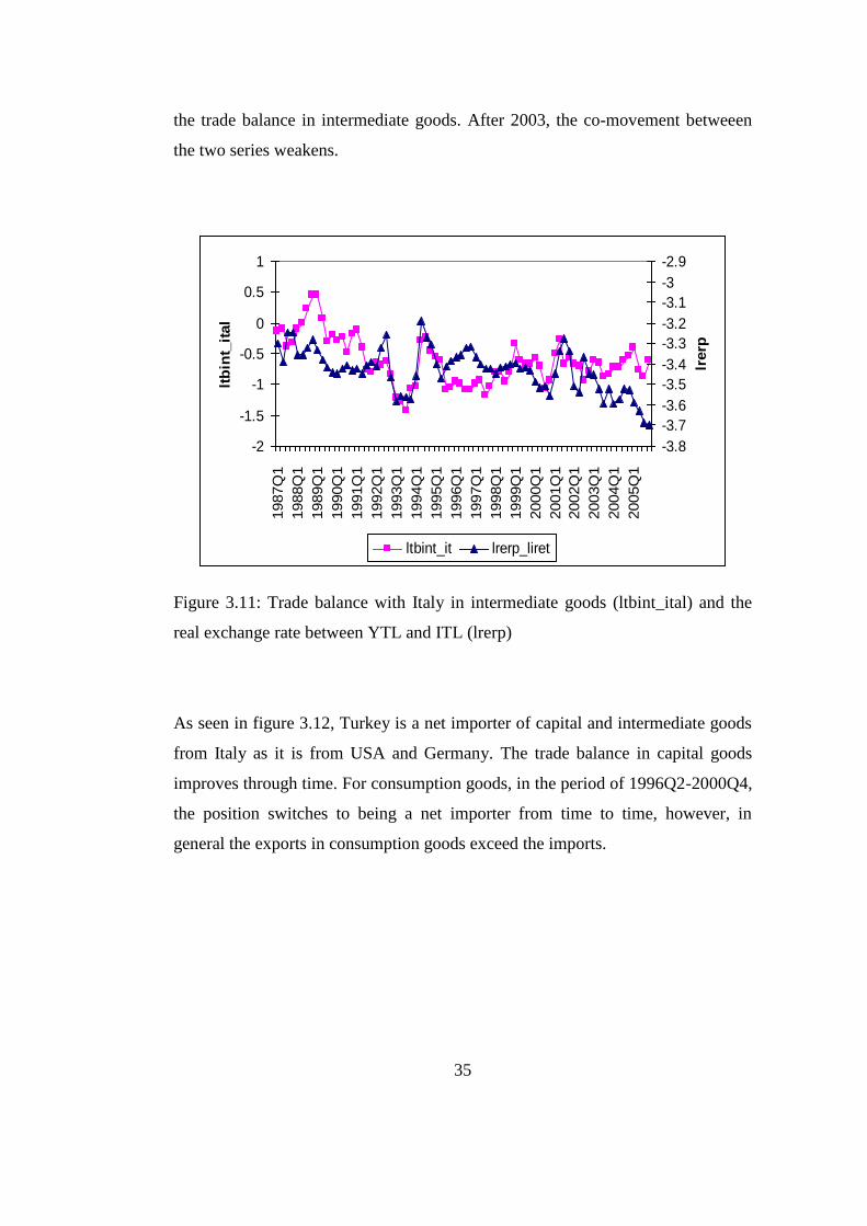
Turkey‟s position as a net exporter or importer of consumption goods. However, it

becomes a net exporter thereafter. As easily observed from figure 2.4, Turkey is a

net importer of capital and intermediate goods from USA throughout the period,

whereas both the trade balances improve through time. Therefore, the production

side of the economy continues to depend on imports of capital and intermediate

goods from US.

Figure 3.5 shows that between 1987Q4-1990Q2, the trade balance with Germany

in consumption goods (LTBCON) follows the movement in the real exchange rate

(LRER). The sharp depreciation in 1994Q4 is followed by a peak in LTBCON in

the following quarter. After the crisis of 1994, the two series broadly move

together. During the period of depreciation in 2001, the contraction in domestic

demand cuts on demand for both domestic products and the imports. As a result,

both the imports fall and the exports rise, leading to improvement of LTBCON.

30

The movement of the trade balance with Germany in capital goods and the real

exchange rate is presented in figure 3.6. It is seen that up to 1989Q3, the trade

balance with Germany in capital goods (LTBCAP) moves in opposite directions

with the real exchange rate (LRERP). Between 1989Q3 and 1994Q1, the two

series seem to be parallel. The sharp depreciation in 1994Q2 causes a peak in

LTBCAP in the next quarter. After 1994Q2, a general appreciation trend is

observed for YTL against DM with the exception of 2000-2001 period. The trade

balance in capital goods, on the other hand, fluctuates around a rising trend.

During the year 2001, the imports of capital goods from Germany falls on

average, as the production side of the economy suffers from a large contraction in

the 2001 crisis. This can be seen in figure 2.6 as the upward movement in

LTBCAP during the year 2001.

Figure 3.7 illustrates that up to 1994Q4, there seems to be a co-movement

between the trade balance with Germany in intermediate goods (LTBINT) and the

real exchange rate (LRERP), although the volatility of LTBINT exceeds the

volatility of LRERP by a considerable amount. During 1994Q2-2000Q4, a

continuous appreciation of YTL against DM is observed; however, LTBINT

fluctuates in different directions. Similar to LTBCAP, depreciation during 2001 is

accompanied by increase in LTBINT, as the production falls due to the economic

crisis. After crisis of 2001, LTBINT and LRERP move in the same direction.

Figure 3.8 reveals that during the sample period Turkey is a net exporter of

consumption goods to Germany and confirms Turkey‟s position as a net importer

of capital and intermediate goods from Germany as well. While the trade balance

in intermediate goods is somewhat stable, the trade balance in capital goods

improves through time and the trade balance in consumption goods decreases.

From figure 3.9, no evidence of a co-movement is seen between the trade balance

with Italy in consumption goods (LTBCON) and the real exchange rate (LRER)

31

up until 1993. During 1993, appreciation of YTL deteriorates LTBCON.

Throughout the period of appreciation of YTL between 1994 and 2000, LTBCON

follows a decreasing trend first, and then fluctuates. During the crisis in 2001,

contraction in domestic demand for both domestic and foreign consumption goods

leads domestic producers to export their products to German market more. On the

other hand, domestic consumers demand less of German consumption goods,

resulting in fall in imports. Consequently, similar to LTBCON with Germany,

LTBCON with Italy improves in 2001. After the crisis, LTBCON and LRER

broadly move in opposite directions.

0.0

0.5

1.0

1.5

2.0

2.5

3.0

3.5

1987Q

1

1988Q

1

1989Q

1

1990Q

1

1991Q

1

1992Q

1

1993Q

1

1994Q

1

1995Q

1

1996Q

1

1997Q

1

1998Q

1

1999Q

1

2000Q

1

2001Q

1

2002Q

1

2003Q

1

2004Q

1

2005Q

1

ltbcon_germ

-1.6

-1.4

-1.2

-1

-0.8

-0.6

-0.4

-0.2

0

lrer

ltbcon_germ lrer_dm

Figure 3.5: Trade balance with Germany in consumption goods (ltbcon_germ)

and the real exchange rate between YTL and DM (lrer)

32

-6

-5

-4

-3

-2

-1

0

1987Q

1

1988Q

1

1989Q

1

1990Q

1

1991Q

1

1992Q

1

1993Q

1

1994Q

1

1995Q

1

1996Q

1

1997Q

1

1998Q

1

1999Q

1

2000Q

1

2001Q

1

2002Q

1

2003Q

1

2004Q

1

2005Q

1

ltbcap_germ

-1.6

-1.4

-1.2

-1

-0.8

-0.6

-0.4

-0.2

0

lrerp

ltbcap_germ lrerp_dm

Figure 3.6: Trade balance with Germany in capital goods (ltbcap_germ) and the

real exchange rate between YTL and DM (lrerp)

-2

-1.6

-1.2

-0.8

-0.4

0

1987Q

1

1988Q

1

1989Q

1

1990Q

1

1991Q

1

1992Q

1

1993Q

1

1994Q

1

1995Q

1

1996Q

1

1997Q

1

1998Q

1

1999Q

1

2000Q

1

2001Q

1

2002Q

1

2003Q

1

2004Q

1

2005Q

1

ltbint_germ

-1.6

-1.4

-1.2

-1

-0.8

-0.6

-0.4

-0.2

0

lrerp

ltbint_germ lrerp_dm

Figure 3.7: Trade balance with Germany in intermediate goods (ltbint_germ) and

the real exchange rate between YTL and DM (lrerp)

33

-6

-4

-2

0

2

4

1987Q

1

1988Q

1

1989Q

1

1990Q

1

1991Q

1

1992Q

1

1993Q

1

1994Q

1

1995Q

1

1996Q

1

1997Q

1

1998Q

1

1999Q

1

2000Q

1

2001Q

1

2002Q

1

2003Q

1

2004Q

1

2005Q

1

ltbcon_germ ltbcap_germ ltbint_germ

Figure 3.8: Trade balance with Germany in consumption, capital and intermediate

goods

-1

-0.5

0

0.5

1

1.5

2

2.5

1987Q

1

1988Q

1

1989Q

1

1990Q

1

1991Q

1

1992Q

1

1993Q

1

1994Q

1

1995Q

1

1996Q

1

1997Q

1

1998Q

1

1999Q

1

2000Q

1

2001Q

1

2002Q

1

2003Q

1

2004Q

1

2005Q

1

ltb

co

n_it

al

-4

-3.5

-3

-2.5

-2

-1.5

-1

-0.5

0

lrer

ltbcon_ital lrer_liret

Figure 3.9: Trade balance with Italy in consumption goods (ltbcon_ital) and the

real exchange rate between YTL and ITL (lrer)

34

Figure 3.10 illustrates that until 1991Q1 the trade balance with Italy in capital

goods (LTBCAP) moves in the opposite direction to the real exchange rate

(LRERP). As the exchange rate appreciates between 1994 and 2001, LTBCAP

improves. During 2001, the economic crisis causes production sector of Turkey to

contract, resulting in a decrease in imports of capital goods, and an improvement

in LTBCAP with Italy similar to the behaviour of LTBCAP with Germany.

However, after 2001, the exchange rate continues to appreciate while LTBCAP

stagnates.

-5

-4.5

-4-3.5

-3

-2.5

-2

-1.5-1

-0.5

0

1987Q

1

1988Q

1

1989Q

1

1990Q

1

1991Q

1

1992Q

1

1993Q

1

1994Q

1

1995Q

1

1996Q

1

1997Q

1

1998Q

1

1999Q

1

2000Q

1

2001Q

1

2002Q

1

2003Q

1

2004Q

1

2005Q

1

ltb

cap

_it

al

-3.8

-3.7

-3.6

-3.5

-3.4

-3.3

-3.2

-3.1

-3

-2.9

lrerp

ltbcap_ital lrerp_liret

Figure 3.10: Trade balance with Italy in capital goods (ltbcap_ital) and the real

exchange rate between YTL and ITL (lrerp)

Figure 3.11 indicates that there is a co-movement between the trade balance with

Italy in intermediate goods (LTBINT) and the real exchange rate (LRERP) during

1988Q2-2002Q3. Similar to LTBINT with Germany, the crisis periods reduces

the imports of intermediate goods as the domestic production falls, and improves

35

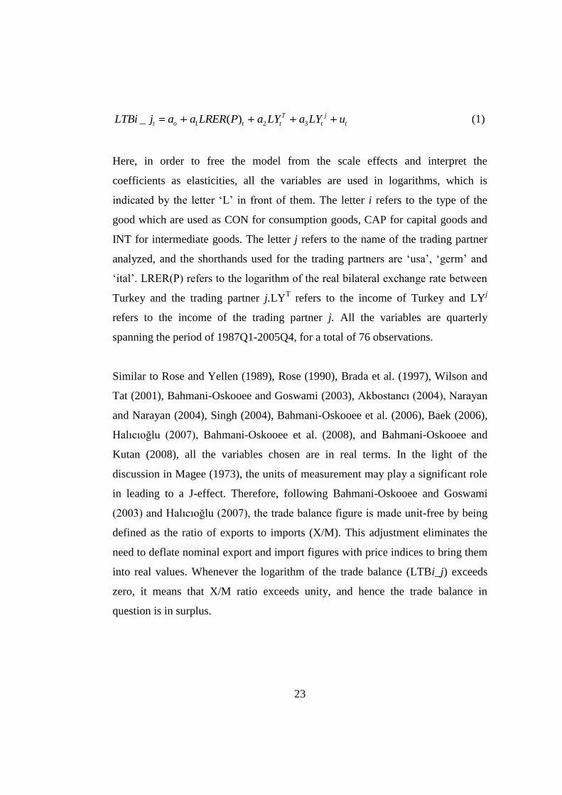
the trade balance in intermediate goods. After 2003, the co-movement betweeen

the two series weakens.

-2

-1.5

-1

-0.5

0

0.5

11987Q

1

1988Q

1

1989Q

1

1990Q

1

1991Q

1

1992Q

1

1993Q

1

1994Q

1

1995Q

1

1996Q

1

1997Q

1

1998Q

1

1999Q

1

2000Q

1

2001Q

1

2002Q

1

2003Q

1

2004Q

1

2005Q

1

ltb

int_

ital

-3.8

-3.7

-3.6

-3.5

-3.4

-3.3

-3.2

-3.1

-3

-2.9

lrerp

ltbint_it lrerp_liret

Figure 3.11: Trade balance with Italy in intermediate goods (ltbint_ital) and the

real exchange rate between YTL and ITL (lrerp)

As seen in figure 3.12, Turkey is a net importer of capital and intermediate goods

from Italy as it is from USA and Germany. The trade balance in capital goods

improves through time. For consumption goods, in the period of 1996Q2-2000Q4,

the position switches to being a net importer from time to time, however, in

general the exports in consumption goods exceed the imports.

36

-5

-4

-3

-2

-1

0

1

2

3

1987Q

1

1988Q

1

1989Q

1

1990Q

1

1991Q

1

1992Q

1

1993Q

1

1994Q

1

1995Q

1

1996Q

1

1997Q

1

1998Q

1

1999Q

1

2000Q

1

2001Q

1

2002Q

1

2003Q

1

2004Q

1

2005Q

1

ltbcon_ital ltbcap_ital ltbint_it

Figure 3.12: Trade balance with Italy in consumption, capital and intermediate

goods

In figures 3.13, 3.14, and 3.15, the sizes of the trade with different trading partners

on each good are compared. As seen from figure 3.13, except for the beginning of

the sample period for USA, Turkey is a net exporter of consumption goods to all

three trading partners. Trade balances of all three countries make a peak during

the crisis of 1994, as domestic demand gets smaller. As Utkulu and Seymen

(2004) explain, with the implementation of Customs Union (CU) from January

1996 onwards, the imports of consumption goods from European countries rise

more than the exports to those countries. The main reason for the greater impact

on imports rather than exports was, as Utkulu and Seymen (2004) mention, was

the parties‟ signature of Additional Protocol on September 1, 1971, before

Customs Union came into effect. This protocol freed exports of some of the

industrial products from Turkey into European market from tariffs starting from

1971. Hence, the CU did not boost exports sharply (Utkulu and Seymen 2004).

Instead, its effect on imports of consumption goods was more evident. The effect

37

is seen from figure 3.13 as well. Up to 1996Q1, Turkey‟s trade in consumption

goods with Germany exceeds the other two countries. However from 1996Q1

onwards, trade with USA catches up with Germany. The trade balance in

consumption goods with Italy deteriorates during 1996-1997, as well.

-2

-1

0

1

2

3

4

1987Q

1

1988Q

1

1989Q

1

1990Q

1

1991Q

1

1992Q

1

1993Q

1

1994Q

1

1995Q

1

1996Q

1

1997Q

1

1998Q

1

1999Q

1

2000Q

1

2001Q

1

2002Q

1

2003Q

1

2004Q

1

2005Q

1

ltbcon_usa ltbcon_germ ltbcon_ital

Figure 3.13: Trade balance in consumption goods with USA, Italy and Germany

Figure 3.14 shows that the trade balance in capital goods moves from a deep

deficit to a smaller one for all the trading partners. This may be due to less

reliance on imports for capital goods or substituting new trading partners in order

to meet the need for capital goods. The size of the trade deficit is greater for USA

at the beginning but it seems to be equalized for all three trading partners through

time. The implementation of CU from January 1996 onwards did not cause a

major impact on LTBCAP with Germany and Italy.

38

-10

-8

-6

-4

-2

0

2

1987Q

1

1988Q

1

1989Q

1

1990Q

1

1991Q

1

1992Q

1

1993Q

1

1994Q

1

1995Q

1

1996Q

1

1997Q

1

1998Q

1

1999Q

1

2000Q

1

2001Q

1

2002Q

1

2003Q

1

2004Q

1

2005Q

1

ltbcap_usa ltbcap_germ ltbcap_ital

Figure 3.14: Trade balance in capital goods with USA, Italy and Germany

-3

-2.5

-2

-1.5

-1

-0.5

0

0.5

1

1987Q

1

1988Q

1

1989Q

1

1990Q

1

1991Q

1

1992Q

1

1993Q

1

1994Q

1

1995Q

1

1996Q

1

1997Q

1

1998Q

1

1999Q

1

2000Q

1

2001Q

1

2002Q

1

2003Q

1

2004Q

1

2005Q

1

ltbint_usa ltbint_germ ltbint_it

Figure 3.15: Trade balance in intermediate goods with USA, Germany and Italy

39

The trade balance in intermediate goods is in deficit with USA, Germany and Italy

as seen in figure 3.15. However, surprisingly, all three balances have a tendency

to improve through the sample period, although the dependency of Turkish

producer on imports of intermediate goods does not change much. This

improvement may be due to increasing share of other trading partners in the total

imports of intermediate goods, such as Russia and China. The trade balance in

intermediate goods becomes relatively stable for all three countries after 1995Q4.

Still, Turkey is a net importer of the intermediate goods from USA, Germany and

Italy.

3.3. Unit Root Tests

The bounds testing approach of Pesaran et al. (2001) allows the variables to be

either stationary or integrated of order one. However, bounds testing can not be

applied if the variables‟ order of integration is either two or higher. To determine

the order of integration, Augmented Dickey Fuller (ADF) tests are applied to the

levels and the first differences. The letter „D‟ indicates that the variable is

differenced once. The results are given in tables 3.1, 3.2, 3.3, 3.4, 3.5, and 3.611

:

As seen from table 3.1, the results support that LTBCAP is stationary and

LTBINT is trend-stationary. Table 3.2 supports that all the variables for US are

stationary when they are differenced once. Since none of the variables is found to

be integrated of order two, bounds testing can be used to test cointegration for

trade balance with USA on all types of goods.

Table 3.3 shows that, when trend is included, hypothesis of having a unit root is

strongly rejected (at 99%) for LTB_CAP while it can not be rejected when it is

excluded. Therefore, LTB_CAP seems to be trend-stationary. Having a unit root

is rejected for LTB_INT for 99% confidence level, so LTB_INT is stationary.

11

The critical values for ADF tests are taken from Greene (2003), Econometric Analysis, New:

Jersey: Pearson Education, p.638

40

Therefore except for LTB_CAP and LTB_INT, the other variables are found to be

I(1) as illustrated by Table 3.4.

Since having a unit root is rejected at 99% confidence level for LTB_CAP, LRER

and LRERP when trend term is included, LTB_CAP, LRER and LRERP are

concluded to be trend-stationary for Italy according to the results in Table 3.5.

When Table 3.6 is examined, all variables are found to be stationary when their

first differences are taken. Therefore, similar to US and German variables, the

variables of Italy are appropriate to conduct a bounds test for cointegration

Table 3.1: ADF test results for levels of variables for USA

With trend and intercept With intercept only

Variables Lags Calculated ADF Lags Calculated ADF

LTB_CON 4 -2.300 4 -1.727

LTB_CAP 0 -5.856*** 0 -3.397*

LTB_INT 4 -3.622** 3 -0.918

LRER 1 -2.571 1 -2.274

LRERP 1 -2.271 1 -2.343

LY 2 -2.357 2 -0.222

Note: The critical values for the models with trend and intercept are -4.04, -3.45, and -

3.15 for confidence levels of 99%, 95% and 90% respectively. The critical values with

intercept only are -3.50, -2.90, and 2.58 for confidence levels of 99%, 95% and 90%

respectively. Rejection of null hypothesis is shown with * for 90%, ** for 95% and ***

for 99% confidence levels.

41

Table 3.2: ADF test results for first differences of variables for USA

With intercept only Without intercept and trend

Variables Lags Calculated ADF Lags Calculated ADF

DLTB_CON 3 -4.723*** 3 -4.676***

DLTB_CAP 1 -10.622*** 0 -10.563***

DLTB_INT 2 -13.637*** 2 -13.692***

DLRER 1 -7.100*** 1 -7.043***

DLRERP 0 -6.999*** 0 -7.041***

DLY 1 -3.700*** 1 -1.787*

Note: The critical values for the models with intercept only are -3.50, -2.90, and 2.58 for

confidence levels of 99%, 95% and 90% respectively. The critical values without an

intercept and trend are -2.60, -1.95, and -1.61 for confidence levels of 99%, 95% and

90% respectively. Rejection of null hypothesis is shown with * for 90%, ** for 95% and

*** for 99% confidence levels.

Table 3.3: ADF test results for levels of variables for Germany

With trend and intercept With intercept only

Variables Lags Calculated ADF Lags Calculated ADF

LTB_CON 5 -3.282* 5 -0.973

LTB_CAP 0 -7.465*** 1 -1.699

LTB_INT 0 -4.418*** 0 -4.323***

LRER 0 -2.100 0 -1.171

LRERP 0 -2.033 0 -1.684

LY 0 -1.770 0 -3.065**

Note: The critical values for the models with trend and intercept are -4.04, -3.45, and -

3.15 for confidence levels of 99%, 95% and 90% respectively. The critical values with

intercept only are -3.50, -2.90, -2.58 for confidence levels of 99%, 95% and 90%

respectively. Rejection of null hypothesis is shown with * for 90%, ** for 95% and ***

for 99% confidence levels.

Table 3.4: ADF test results for first differences of variables for Germany

With intercept only Without intercept and trend

Variables Lags Calculated ADF Lags Calculated ADF

DLTB_CON 4 -5.829*** 4 -5.816***

DLTB_CAP 0 -14.519*** 0 -14.574***

DLTB_INT 6 -5.379*** 6 -5.408***

DLRER 0 -7.255*** 0 -7.222***

DLRERP 0 -7.615*** 0 -7.639***

DLY 0 -8.221*** 0 -7.126***

Note: The critical values for the models with intercept only are -3.50, -2.90, and 2.58 for

confidence levels of 99%, 95% and 90% respectively. The critical values without an

intercept and trend are -2.60, -1.95, and -1.61 for confidence levels of 99%, 95% and

90% respectively. Rejection of null hypothesis is shown with * for 90%, ** for 95% and

*** for 99% confidence levels.

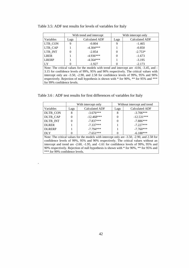
42

Table 3.5: ADF test results for levels of variables for Italy

With trend and intercept With intercept only

Variables Lags Calculated ADF Lags Calculated ADF

LTB_CON 9 -0.804 9 -1.465

LTB_CAP 1 -4.304*** 1 -0.850

LTB_INT 0 -2.854 0 -2.753*

LRER 1 -4.936*** 0 -1.673

LRERP 1 -4.564*** 1 -3.195

LY 0 -1.927 0 -2.173

Note: The critical values for the models with trend and intercept are -4.04, -3.45, and -

3.15 for confidence levels of 99%, 95% and 90% respectively. The critical values with

intercept only are -3.50, -2.90, and 2.58 for confidence levels of 99%, 95% and 90%

respectively. Rejection of null hypothesis is shown with * for 90%, ** for 95% and ***

for 99% confidence levels.

Table 3.6 : ADF test results for first differences of variables for Italy

With intercept only Without intercept and trend

Variables Lags Calculated ADF Lags Calculated ADF

DLTB_CON 8 -3.676*** 8 -3.706***

DLTB_CAP 0 -12.468*** 0 -12.531***

DLTB_INT 0 -7.837*** 0 -7.886***

DLRER 1 -7.337*** 1 -7.227***

DLRERP 1 -7.794*** 1 -7.760***

DLY 0 -7.651*** 0 -6.188***

Note: The critical values for the models with intercept only are -3.50, -2.90, and 2.58 for

confidence levels of 99%, 95% and 90% respectively. The critical values without an

intercept and trend are -2.60, -1.95, and -1.61 for confidence levels of 99%, 95% and

90% respectively. Rejection of null hypothesis is shown with * for 90%, ** for 95% and

*** for 99% confidence levels.

.

43

CHAPTER 4

THE EMPIRICAL ANALYSIS

As explained in Chapter 2, the analysis of J-curve requires examination of both

the long run and the short run dynamics between the real exchange rate and the

trade balance. The main concern of the analysis in this chapter is finding answers

to some questions summarized below:

Is there a cointegration among the variables chosen?

Is there a significant long run relationship between the trade balance with

country j in good type i (LTBi_j) and the real exchange rate (LRER(P))

Is there a significant short run relationship between the LTBi_j and

LRER(P).

If the answers to the questions above are affirmative, is the direction of the

effect negative for short run and positive for long run, resulting in a J-

shape?

To answer all the questions above, bounds testing approach for cointegration

developed by Pesaran et al. (2001) is used. Preferring bounds testing approach

(Pesaran et al. 2001) for this study mainly depends on two reasons: First of all, it

allows the variables to be stationary, integrated of order one or a mixture of both,

44

which is the characteristics of the data used. Second, as illustrated by Pesaran et

al. (2001), bounds testing for cointegration is proceeded with analysis of an

autoregressive distributed lag model (ARDL) based on Pesaran and Shin (1999).

As a result, the long run and the short run dynamics can be examined as well,

fulfilling the main requirement for a J-curve analysis.

The bounds testing approach (Pesaran et al. 2001) tests the null hypothesis of no

cointegration. In fact, it is mainly a joint significance test of the one period lagged

values of the levels in an unrestricted error correction model (UECM) expressed

as follows:

1 0 0 0

1 1 1 1

_ _ ( )

_ ( )

p p p pT j

t k t k k t k k t k k

k k k k

T j

t t t t t

LTBi j LTBi j LRER P LY LY

LTBi j LRER P LY LY u

(4)

In other words, the first step is to test H0: δ1=δ2=δ3=δ4=0 (the hypothesis of no

cointegration) against the alternative H1: δ1≠0, δ2≠0, δ3≠0, δ4≠0. The calculated

F-statistics has a nonstandard distribution such that for each confidence level, two

critical value bounds are developed: one assuming that all the variables are

stationary and another assuming that all the variables are integrated of order one.

These critical values provide upper and lower bounds to compare the calculated F-

statistic. If the calculated statistics lies above the upper bound, the null hypothesis

of no cointegration is rejected. If the calculated statistic lies below the lower

bound, the null hypothesis can not be rejected. If the calculated F-statistic falls

between the lower and upper bounds, then a conclusion can not be drawn, the

analysis can be carried further into the ECM.

If cointegration is found or at least the results are inconclusive, it becomes

meaningful to analyze the ECM and the short run and the long run dynamics

associated with it. Therefore ARDL approach of Pesaran and Shin (1999) is

45

conducted next and the relationship between the levels are examined with the

ECM derived from that specific ARDL (q,r,s,t).

As first illustrated by Pesaran et al. (2001), the results of the bounds testing

approach are sensitive to the lag length chosen for the first differenced variables.

In order to verify this, the calculated F-statistics for different lags chosen for the

first differences of the variables are given in Table 4.1. Following Pesaran and

Pesaran (1997), the current values of the first differenced explanatory variables

are not included at this stage, as it can not be inferred that those variables are

totally „explanatory‟ rather than being „dependent‟. In other words, calculated F-

statistics presented below are namely F(LTBi | LRER(P), LYT, LY

j) for now. To

present the full picture, the lag lengths are chosen as many as possible, here as 13,

which is the greatest lag length the sample size allows, leaving enough number of

observations in order to carry out a bounds test.

As seen from Table 4.1, the hypothesis of no cointegration between the trade

balance with USA in consumption goods, the real exchange rate, real domestic

income and real foreign income is rejected at different significance levels for lag

orders of 1, 2, 10 and 13.The results are inconclusive for lag orders of 7 and 11.

The hypothesis of no cointegration between the trade balance with USA in capital

goods, the real exchange rate, real domestic income and real foreign income is

rejected at different significance levels for lag orders of 1, 2, 13 while no

conclusion can be drawn for lag orders of 3, 4, 5 and 10. Last of all no

cointegration between the trade balance with USA in intermediate goods, the real

exchange rate, real domestic income and real foreign income is rejected at

different significance levels for lag orders of 1, 2, 9 and 10 while the results are

inconclusive for lag orders of 3, 6, 7 and 11.

Failure to reject the null hypothesis of no cointegration is rarer in the case of

Germany. The results either reject no cointegration or at least remain

46

inconclusive, leaving room to carry the analysis further into error correction

model. For lag orders of 2, 4, 5, 6, 7 and 13, no cointegration is rejected for trade

balance in consumption goods, and for 3, 8 and 10 lags, results are inconclusive.

For lag orders of 1, 3, 4 and 8, no cointegration is rejected for trade balance in

capital goods while the calculated statistics fall into the inconclusive region for

lag orders of 2, 5, 6, 7, 9 and 12. Last of all, the trade balance in intermediate

goods supports cointegration for lags of 1, 2, 3, 4, 8, 10 and 11. The inconclusive

region is seen for lag orders of 5, 7 and 13.

Contrary to Germany, the data for Italy does not reject the null hypothesis of no

cointegration for most of the cases. Only for lag order of 1, for capital goods; and

lag order of 1 and 2 for intermediate goods, no cointegration is rejected. For lag

orders of 2 and 10 for consumption and capital goods and 12 for intermediate

goods, the results of the bounds test are inconclusive.

Following Pesaran et al. (2001), and also illustrated by Islam (2004), the lag

length used for bounds testing is decided by an unrestricted VAR model referring

to the different information criteria, which are Akaike‟s Information Criteria

(AIC) and Schwarz Information Criteria (SC). The suggested lag lengths by AIC

and SC criteria of the unrestricted VAR model are given in table A.1 in Appendix

C. As seen from the table, AIC and SC do not agree on the optimum number of

lags to be included12

. AIC criterion which suggests more lags to be included is

taken into consideration for the rest of the study, as the main focus here is to

analyze short run effects of the real exchange rate to the possible extent.

Therefore, number of lags included for the levels are 8 for LTBCON and

LTBCAP; 5 for LTBINT for USA; 6 for LTBCON, 5 for LTBCAP, and 8 for

LTBINT for Germany; 5 for LTBCON and LTBCAP, 7 for LTBINT for Italy to

carry a bounds test for cointegration.

12

Except for the case of Italy in capital goods.

47

Table 4.1: The calculated F-statistics relevant for bounds test for different lag lengths of the first differenced variables.

USA GERMANY ITALY

Lag Length LTBCON LTBCAP LTBINT LTBCON LTBCAP LTBINT LTBCON LTBCAP LTBINT

1 10.788*** 10.1996*** 8.8238*** 1.9974 5.9659*** 8.2484*** 2.2846 4.5281** 8.1059***

2 4.1771* 3.8625* 9.286*** 11.218*** 3.4601i 6.6171*** 2.9136i 3.3577i 4.9131**

3 1.2673 2.7486i 3.2796i 3.7332i 4.1802* 4.2232* 1.8225 1.5177 1.9547

4 1.3679 3.3699i 2.0955 4.0228* 3.7719* 5.025** 0.74892 1.3207 1.4203

5 1.6831 2.7547i 1.8126 4.4881** 3.1874i 3.3388i 0.89389 1.0129 1.0696

6 1.1319 2.5683 3.4285i 5.166** 3.0609i 2.6971 0.49136 0.54376 1.7535

7 3.1662i 2.5082 2.8719i 4.0821* 2.9156i 3.3893i 0.65417 0.7243 2.4012

8 2.2147 2.0379 2.6669 3.0248i 5.3184** 7.4139*** 1.2617 1.0461 2.3826

9 2.5585 1.5305 3.9499* 2.459 3.6596i 2.6276 0.79747 1.7422 1.824

10 3.8486* 3.5455i 4.744** 3.5844i 2.226 1.4747 2.742i 3.1134i 1.8412

11 3.3376i 2.4057 3.1756i 2.2841 1.3127 5.5045** 1.824 1.7749 1.5568

12 0.95579 1.5973 1.7828 1.497 2.7217i 7.6038*** 1.408 0.91452 3.2354i

13 5.3869** 3.8148* 1.5081 3.7985* 1.717 3.0078i 0.46413 0.36901 1.7269

The critical value bounds to test the null hypothesis of no cointegration are 2.72 and 3.77 for 90%, 3.23 and 4.35 for 95%, 4.29 and 5.61 for 99%

confidence levels (Pesaran et al. 2001, Table CI(iii) Case III). Rejection of null hypothesis is indicated with * for 90%, ** for 95%, and *** for

99% confidence levels, and i denotes inconclusiveness for 90%. Lag length refers to the lags of the first differenced variables.

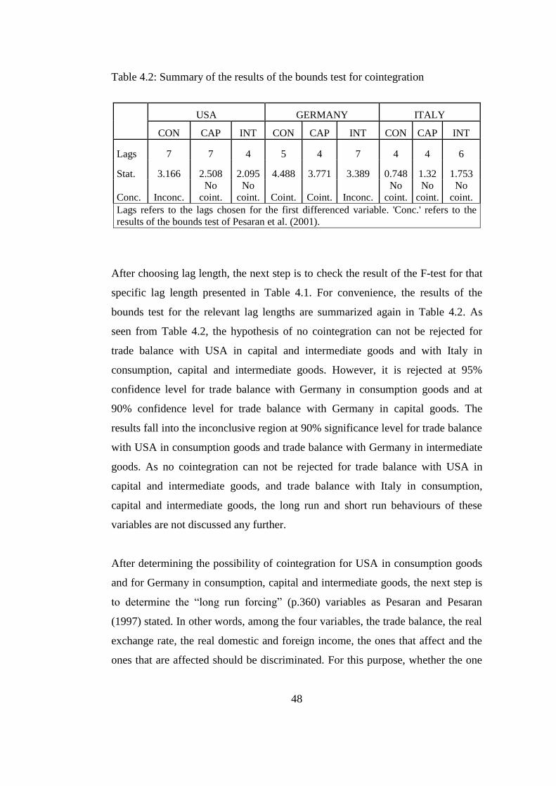
48

Table 4.2: Summary of the results of the bounds test for cointegration

USA GERMANY ITALY

CON CAP INT CON CAP INT CON CAP INT

Lags 7 7 4 5 4 7 4 4 6

Stat. 3.166 2.508 2.095 4.488 3.771 3.389 0.748 1.32 1.753

Conc. Inconc.

No

coint.

No

coint. Coint. Coint. Inconc.

No

coint.

No

coint.

No

coint.

Lags refers to the lags chosen for the first differenced variable. 'Conc.' refers to the

results of the bounds test of Pesaran et al. (2001).

After choosing lag length, the next step is to check the result of the F-test for that

specific lag length presented in Table 4.1. For convenience, the results of the

bounds test for the relevant lag lengths are summarized again in Table 4.2. As

seen from Table 4.2, the hypothesis of no cointegration can not be rejected for

trade balance with USA in capital and intermediate goods and with Italy in

consumption, capital and intermediate goods. However, it is rejected at 95%

confidence level for trade balance with Germany in consumption goods and at

90% confidence level for trade balance with Germany in capital goods. The

results fall into the inconclusive region at 90% significance level for trade balance

with USA in consumption goods and trade balance with Germany in intermediate

goods. As no cointegration can not be rejected for trade balance with USA in

capital and intermediate goods, and trade balance with Italy in consumption,

capital and intermediate goods, the long run and short run behaviours of these

variables are not discussed any further.

After determining the possibility of cointegration for USA in consumption goods

and for Germany in consumption, capital and intermediate goods, the next step is

to determine the “long run forcing” (p.360) variables as Pesaran and Pesaran

(1997) stated. In other words, among the four variables, the trade balance, the real

exchange rate, the real domestic and foreign income, the ones that affect and the

ones that are affected should be discriminated. For this purpose, whether the one

49

period lagged level variables are jointly significant in explaining the real exchange

rate, the real domestic income and the real foreign income is tested separately

using bounds testing approach at lag levels determined above. In other words,

LRER(P), LYT and LY

j are chosen as the dependent variable in equation (4), and

the bounds test is conducted for each separately. The results are given below:

Table 4.3: The results of the bounds test for different dependent variables

USA GERMANY ITALY

Calculated F-stat CON CAP INT CON CAP INT CON CAP INT

LRER|LTBi,LYT,LY

j 1.92 1.09 0.77 1.38 1.36 2.78i 4.10* 2.34 2.63

LYT |LTBi,LRER,LY

j 0.16 0.60 1.65 0.22 2.21 0.35 5.25** 2.09 1.00

LYj |LTBi,LRER,LY

T 2.54 2.41 1.98 2.61 1.78 1.44 1.33 0.85 1.58

The critical value bounds to test the null hypothesis of no cointegration are 2.72 and

3.77 for 90%, 3.23 and 4.35 for 95%, 4.29 and 5.61 for 99% confidence levels

(Pesaran et al. 2001, Table CI(iii) Case III). Rejection of null hypothesis is indicated

with * for 90%, ** for 95%, and *** for 99% confidence levels, and i denotes

inconclusiveness for 90%.

As seen in Table 4.3, the results support that if cointegration is found, that is a

long-run relationship is supported, then among the four variables, it is the trade

balance that is „explained‟ by the other 3 variables. In other words, the real trade

balance is dependent and the real exchange rate, the real foreign income and the

real domestic income are the explanatory ones13

.

In the light of Pesaran et al. (2001), for the cases where the results either reject no

cointegration or at least fall into the inconclusive region, an ARDL(q,r,s,t)

following Pesaran and Shin (1999) is built and the estimates of the relationship

13

The only exception is for Italy in consumption goods. However, as no cointegration is found for

Italy, this result does not have a role on the rest of the study.

50

between levels is examined. Accordingly, in this study the long run relationship is

examined next and the results are presented in Table 4.4.

Table 4.4: The long run estimates of the relationship between the levels

USA GERMANY

LTBCON LTBCON LTBCAP LTBINT

Reg. Coef. Prob. Coef. Prob. Coef. Prob. Coef. Prob.

Intercept -14.59*** 0.000 10.63*** 0.001 -16.95*** 0.000 -3.81** 0.026

LRER(P) 1.91*** 0.002 0.02 0.964 -0.18 0.802 -0.38 0.252

LYT 5.93** 0.016 -2.47*** 0.009 2.63** 0.045 0.44 0.307

LYj -2.19 0.415 1.13 0.719 1.36 0.752 0.11 0.946

„Reg.‟ refers to the name of the regressors. Significance at 90%, 95%, and 99% is

denoted by *,**,and*** respectively.

The results show that foreign real income is not a significant variable for affecting

trade balance on any type of good in the long run. The trade balance seems not to

depend on demand or supply side factors from other countries, but instead is

mainly determined domestic demand and domestic supply factors.

The real exchange rate (LRER) is only significant for explaining the trade balance

in consumption goods (LTBCON) with USA. The behaviour is in line with the

expectations of the theory: increase in LRER, i.e. depreciation of YTL, improves

the LTBCON with USA in the long run.

The significance of the LYT varies across different types of tradables. For

consumption goods for both USA and Germany, the LYT is significant. However,

the direction of its effect differs. For LTBCON with USA, the supply side factors

seem to dominate in the long run, that is, as domestic income rises, supply of

exports of consumption goods increases by more than the demand for imports of

consumption goods, and trade balance improves accordingly. However, for

51

Germany, demand side factors seem to dominate, as the increase in LYT is

accompanied by deterioration of LTBCON.

The results are surprising, when trade balance with Germany in capital and

intermediate goods are examined. Rise in LYT triggers increases in the supply of

exportable capital goods by more than increases in demand for imports of capital

goods. Contrary to expectations, the growth in the economy does not seem to

force producers to import more capital goods. Instead, the economic growth

causes exports of capital goods to increase. However, the trade balance in

intermediate goods with Germany does not depend on domestic real income in the

long run.

After examination of the levels relationship, the ECMs derived from the

underlying ARDL (q,r,s,t) model given in equation (5) are analyzed for short run

dynamics. The variables included and their coefficients are presented in Table.4.5.

1 0 0 0

_ _ ( )q r s t

T j

t k t k k t k k t k k

k k k k

LTBi j LTBi j LRER P LY LY (5)

As the results of the ARDL based ECMs show, the error correction term (ECT) is

negative and highly significant in all 4 cases, which means deviations from long

run equilibrium is corrected through time. Therefore, ECM supports the results of

the bounds test for existence of cointegration for the 4 cases above. However, the

real exchange rate is insignificant with all its lags in all of the cases considered.

In the short run, trade balance in consumption goods with USA mainly depends

on DLYT. As seen above the DLY

T and its values for lag levels of 1,2, 5 and 7

are highly significant and all have a negative coefficient. In other words, contrary

to the long run impact, an increase in domestic income worsens the trade balance

with USA in consumption goods in the short run. The difference in the direction

of the response of the trade balance in consumption goods may be explained with

52

the different supply elasticities in the short run and the long run. The increase in

domestic income in the short run causes domestic demand for consumption goods

to rise. As expected, the supply of goods is more inflexible in the short run, as a

result, this excess demand can not be met immediately with domestic resources.

Instead, the imports of consumption goods rises, leading to a deterioration in the

trade balance in consumption goods. However, in the long run, the passage of

time allows the producers to make the necessary preparations to meet this excess

demand and to shift more resources to increase production of consumption goods.

With this expansion in production, supply of exportable consumption goods

increases as well, leading to an improvement in the trade balance in the long run.

The trade balance in consumption goods with USA also depends on 2 and 7

period lagged values of the DLYj. In other words, increase in US income causes

LTBCON to increase with a lag of 2 or 7 periods that is 0.5 to 1.5 years

approximately. The reasoning may be similar to the case of increased domestic

income. As the US income rises, US demand increases. In the short run, it may be

impossible to meet this excess demand with home-country resources, so imports

from Turkey rises, contributing to the improvement of the Turkish trade balance

in consumption goods. However, in the long run, the domestic resources may be

adjusted properly to meet increased domestic demand in the US. As a result, in the

long run, the movements in the foreign income becomes irrelevant for Turkey‟s

trade balance.

Last of all, the 4 period lagged value of DLTBCON is also a significant variable

in the short run. Increases in the difference between current and the previous

period‟s LTBCON affects LTBCON positively in the following fourth period.

The results are more disappointing for LTBCON with Germany. The variables

chosen are cointegrated, so there exists a long run relationship between these

variables. However, in the short run, neither of these variables seem to have a

significant effect on the LTBCON, except for DLYT(t-3). As seen above, only

53

DLYT(t-3) is significant and it is negative. So, three quarters after the increase in

domestic income, LTBCON deteriorates, similar to its long run response. For

trade in consumption goods with Germany, demand side effects dominate both in

the short run and the long run. Domestic income growth triggers imports instead

of increasing the supply of exports.

For LTBCAP with Germany, the domestic income variable is significant with all

of its lags in the short run as it is in the long run. However, while the long run

coefficient is positive, the coefficients of all its lags are negative in the short run.

Increases in domestic income necessitate increases in production for some sectors.

However, this expansion requires more capital goods to be imported in the short

run, rationalizing the negative coefficients in front of the domestic income figures.

However, in the long run, Turkey seems to increase its production of exportable

capital goods to Germany. As a result, the trade balance in capital goods

improves. The change in foreign income is significant at its 1 and 2 period lagged

values. The one period lagged DLYj deteriorates the LTBCAP while the 2 period

lagged DLYj improves it.

While the domestic income is insignificant in the long run in explaining LTBINT

with Germany, all its lags are found to be significant in the short run. Similar to

LTBCAP with Germany, increases in domestic income requires expansion in the

production, causing imports of intermediate goods to rise and LTBINT to

deteriorate. However, in the long run, fluctuations in domestic income are

irrelevant to the movements in the LTBINT. The other variables, the real

exchange rate and the foreign income, are found to be insignificant in the short

run as they are in the long run.

54

Table 4.5: Estimated short run coefficients of the variables

USA GERMANY

LTBCON LTBCON LTBCAP LTBINT

ARDL (5,1,8,8) ARDL (4,2,4,0) ARDL (2,0,4,3) ARDL (1,1,5,0)

Regressors Coef. Prob. Coef. Prob. Coef. Prob. Coef. Prob.

DLTBi(t-1) -0.064 0.727 0.11 0.421 -0.164 0.166

DLTBi(t-2) -0.016 0.921 0.222 0.101

DLTBi(t-3) -0.174 0.233 -0.173 0.155

DLTBi(t-4) 0.26014** 0.029

DLRER(P)(t) 0.371 0.689 0.646 0.126 -0.102 0.804 0.500 0.167

DLRER(P)(t-1) 0.528 0.205

DLYT (t) -3.836** 0.028 -1.076 0.129 -2.039** 0.015 -0.961* 0.055

DLYT (t-1) -5.160** 0.016 -1.008 0.225 -3.471*** 0.000 -1.736*** 0.001

DLYT (t-2) -6.488** 0.001 -0.435 0.575 -2.470*** 0.004 -1.505*** 0.002

DLYT (t-3) -1.797 0.319 -1.441** 0.042 -2.284*** 0.005 -1.608*** 0.001

DLYT (t-4) -2.890 0.102 -0.753 0.135

DLYT (t-5) -5.039*** 0.003

DLYT (t-6) -2.976* 0.052

DLYT (t-7) -5.964*** 0.000

Significance of the variables are indicated with * for 90%, ** for 95%, and *** for 99% confidence levels.

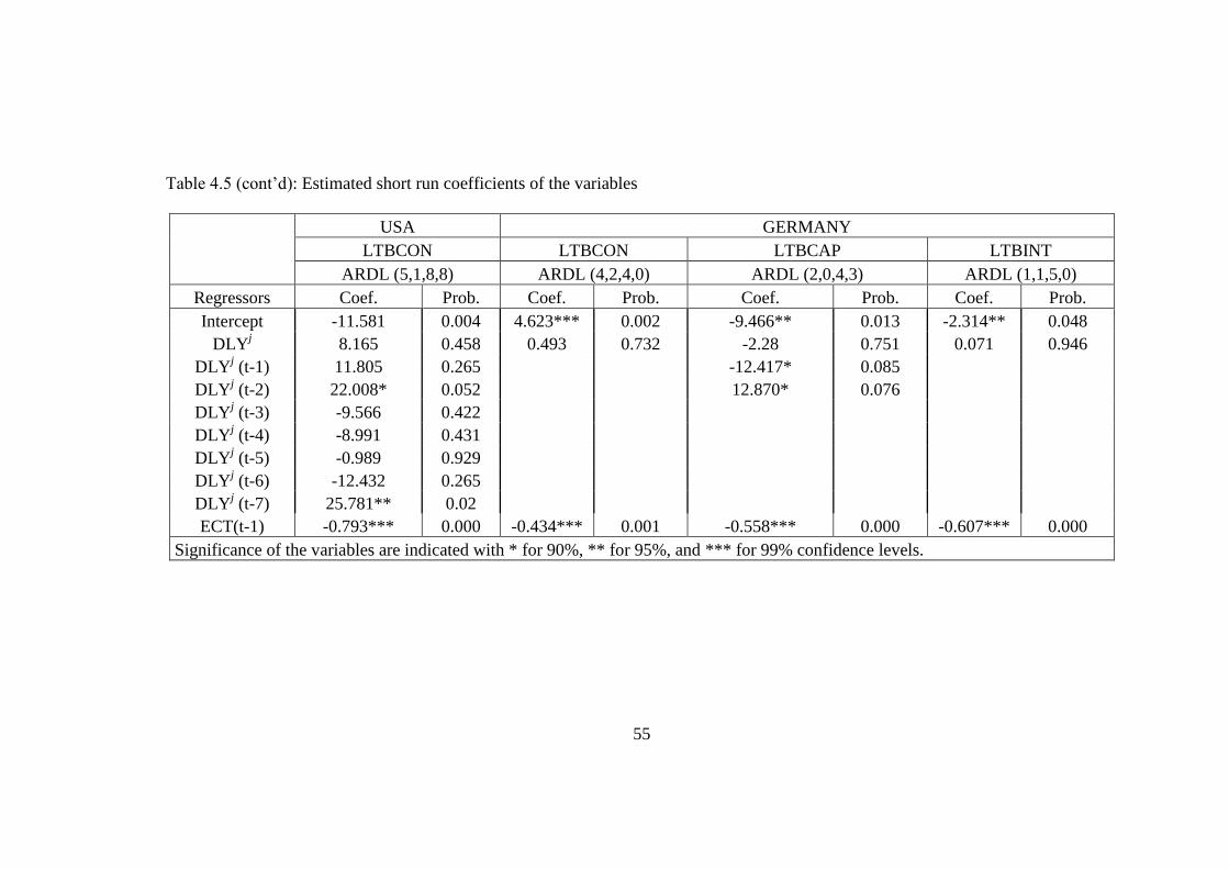
55

Table 4.5 (cont‟d): Estimated short run coefficients of the variables

USA GERMANY

LTBCON LTBCON LTBCAP LTBINT

ARDL (5,1,8,8) ARDL (4,2,4,0) ARDL (2,0,4,3) ARDL (1,1,5,0)

Regressors Coef. Prob. Coef. Prob. Coef. Prob. Coef. Prob.

Intercept -11.581 0.004 4.623*** 0.002 -9.466** 0.013 -2.314** 0.048

DLYj 8.165 0.458 0.493 0.732 -2.28 0.751 0.071 0.946

DLYj (t-1) 11.805 0.265 -12.417* 0.085

DLYj (t-2) 22.008* 0.052 12.870* 0.076

DLYj (t-3) -9.566 0.422

DLYj (t-4) -8.991 0.431

DLYj (t-5) -0.989 0.929

DLYj (t-6) -12.432 0.265

DLYj (t-7) 25.781** 0.02

ECT(t-1) -0.793*** 0.000 -0.434*** 0.001 -0.558*** 0.000 -0.607*** 0.000

Significance of the variables are indicated with * for 90%, ** for 95%, and *** for 99% confidence levels.

56

As explained above, depreciation of the real exchange rate causes an improvement

only in trade balance with USA in consumption goods. In the short run, the real

exchange rate is not found to be a significant factor in any of the four cases

considered. Thus, contrary to expectations, the real exchange rate has no role in

the short run on trade balance with USA in consumption goods, and trade balance

with Germany in consumption, capital and intermediate goods. Hence, discussion

of different responses of the trade balance to the movement in the real exchange

rate in the short and the long run is totally meaningless. The trade balance with

USA in consumption goods and with Germany in consumption, capital and

intermediate goods do not support the J-curve. The trade balances even stay

unresponsive to fluctuations in the real exchange rate both in the short run and in

the long run14

.

14

Except for the trade balance with USA in consumption goods.

57

CHAPTER 5

CONCLUSIONS

The exchange rate is one of the easiest ways to make quick overall assessments

about the country‟s position with respect to international competitiveness.

Through its effect on relative prices, it is expected to be one of the most important

determinants of trade balance in an open economy. While increases in capital

mobility, development of new financial instruments against capital controls, and

shifts to other price stabilization policies such as inflation targeting from

exchange rate targeting reduce countries‟ control on the value of their currencies,

the exchange rate is expected to have a significant role on the trade balances. The

fact that domestic currencies of developing countries are more susceptible to

global risks and more unpredictable throughout the world is another motivator

behind this study which aims to build an empirical link between the real exchange

rate and the trade balance.

Besides the significance of the movements of the real exchange rate on the

movements of the trade balance, the different responses of the trade balance in the

short run and the long run is the main concern of this study. Assuming that the

Marshall-Lerner condition holds, weakening domestic currency against trading

partners‟ currencies is expected to boost exports and discourage imports, leading

to an improvement. However, as Magee (1973) suggests, the immediate short run

response of the trade balance may be to deteriorate due to already signed contracts

or low pass-through from exchange rate to the tradable prices. Hence, as he

58

mentions, the trade balance may follow a path resembling the letter „J‟, named as

J-curve effect. Knowing whether the deterioration is temporary or not, is

important for both diagnosis and the remedies of the problem.

Going through the literature in this area, there seems to be a gap in terms of

bilateral analysis for Turkey. To the best of knowledge, Halıcıoğlu (2007) is the

only study at bilateral level. Hence, this study analyzes the bilateral trade data of

Turkey with her three major trading partners; USA, Germany and Italy. Moreover,

in order to eliminate problems associated with using aggregate data, the trade

balance in different types of goods according to BEC definition of United

Nations. This definition classifies the tradables according to their main end use as

consumption, capital and intermediate goods. This disaggregation is expected to

prevent movements in each group in different directions to offset each other.

Moreover, this disaggregation provides a chance to compare the impact of supply

side factors and demand side factors as the trade balance in capital and

intermediate goods are expected to reflect the production side whereas trade

balance in consumption goods is expected to reflect the demand side of the

economy.

In the empirical analysis, quarterly data is used covering the trade balance in

consumption, capital and intermediate goods with USA, Germany and Italy and

spans the period of 1987-2003 for a total of 76 observations. Following Rose and

Yellen (1989), which is followed by majority of the literature, the trade balance is

regressed on the real bilateral exchange rate, the real domestic income and the real

foreign income. Increases in the exchange rate (defined as domestic currency

price of the one unit of foreign currency) are expected to improve the trade

balance in the long run. However, no expectations are assigned to the signs of the

coefficients of the income variables in advance, as the direction of their effects

would depend on the dominance of the demand or supply side factors.

59

Considering that the variables used are either stationary or integrated of order one,

the bounds testing approach developed by Pesaran, Shin and Smith (2001) is used.

Morover, following Pesaran et al. (2001), the analysis continues with ARDL

approach of Pesaran and Shin (1999), which gives both the short run and long run

dynamics of the variables. This enables a complete J-curve analysis, as both the

short run and the long run response of the trade balance is investigated.

The results of the bounds test (Pesaran et al. 2001), supported cointegration

among all the variables included in the model for trade balance with Germany in

consumption and capital goods. The results are inconclusive for trade balance

with USA in consumption goods and trade balance with Germany in intermediate

goods. The case of USA in capital and intermediate goods and Italy in

consumption, capital and intermediate goods do not support cointegration among

the variables in the model. However, J-curve analysis requires examination of

both the short run and the long run dynamics. As the results of the bounds test do

not suggest long run relationship among the variables, the short run dynamics are

not analyzed any further for the cases mentioned above. The direction of the

cointegration is searched next. Following Pesaran and Pesaran (1997), the “long

run forcing” variables (p.360) are found to be the real exchange rate, the domestic

real income and the foreign real income.

Next, the long run and the short run dynamics are analyzed. The real exchange

rate is found to be a significant variable only in explaining the trade balance with

USA in consumption goods. As expected, depreciation is found to improve the

trade balance in consumption goods. The foreign real income is found to be

insignificant in all the four cases. The domestic real income is found to be

significant for trade balance with USA in consumption goods, trade balance with

Germany in consumption and capital goods; and insignificant for trade balance

with Germany in intermediate goods. Increases in domestic income cause demand

side factors to dominate for trade balance with USA in consumption goods and

the trade balance with Germany in capital goods. In other words, increases in

60

domestic income improve the trade balances mentioned. However, increases in

domestic income deteriorate the trade balance with Germany in consumption

goods.

The real exchange rate is totally insignificant with all its lags in the short run for

all the four cases analyzed. For trade balance with USA in consumption goods,

nearly all the lags of the domestic real income is significant and negative,

indicating that income growth causes trade balance with USA in consumption

goods to deteriorate in the short run. The two lags of the foreign real income are

significant and carry negative signs.

The only significant factor in the short run for trade balance with Germany in

consumption goods is three period lagged value of the first differenced real

domestic income. Increases in income cause the trade balance with Germany in

consumption goods to deteriorate, similar to its long run effect.

Increases in real domestic income are found to worsen the trade balance with

Germany in capital goods. Two of the lagged values of the first differences of the

real foreign income are significant; however, they affect the trade balance in

different ways.

Increases in real domestic income are found to deteriorate the trade balance with

Germany in intermediate goods, as expected. No other variable has a short run

effect on the trade balance with Germany in intermediate goods.

The empirical analysis suggests that contrary to expectations, the real exchange

rate is not a significant variable either in the long run, except for the trade balance

with USA in consumption goods, or in the short run. Therefore, J-curve effect is

not evident for Turkey‟s bilateral trade with USA, Germany and Italy in

consumption, capital and intermediate goods. This finding implies that the real

exchange rate shocks are not reflected to the bilateral trade balances. Another

61

explanation is that exchange rate pass-through to import and export prices are low

so that exports and imports are not responsive to the exchange rate fluctuations.

However, this explanation rationalizes results of the short run analysis. In the long

run, pass-through is expected to be realized more.

One more reason may be that the period considered (1987-2005) includes several

macroeconomic crises and structural shocks that might cause different behaviours

of the trade balance in different subperiods. For instance, two serious economic

crises of 1994 and 2001, and the earthquake of 1999 caused production to slow

down and the economy to contract. Moreover, the introduction of euro in 1999

affected currency denomination of imports. As seen in Chapter 3, the trade

balances and the real exchange rates act in different ways for those different

subsample periods. For instance, for trade balance with Germany in capital goods

and the real exchange rate, the two series move in opposite directions after the

crisis of 1994, while co-movement is observed for the period of 1990-1994. Or for

the case of Germany in intermediate goods, no pattern can be observed for the

period of 1994-2000, while after 2001 crisis, the two series broadly move

together. In short, observing sub-sample periods separately may suggest a more

important role for the real exchange rate in affecting the trade balance. Further

research in this area may try looking at the trade balance-exchange rate

relationship in for pre and post crises periods and for the period of transition to

euro.

The insignificance of the bilateral real exchange rate may be due to the fact that

Turkey exports mostly in euros and imports mostly in dollars, as Berument and

Dinçer (2005) explain. Therefore, following their study, the euro-dollar parity

may be the significant factor in explaining the trade balances rather than the

bilateral exchange rates. On the other hand, the euro-dollar parity may reflect the

competition between the largest import suppliers of Turkey; Germany , USA and

Italy. Therefore rather than substituting the bilateral exchange rate with the euro-

62

dollar parity, that rate may be incluede in the model along with the bilateral rates

to account for the third country effects as Rose and Yellen (1989) mention.

In short, the results of this study suggest that the real exchange rate is not a

significant variable in explaining the behaviour of bilateral trade balance of

Turkey in consumption, capital and intermediate goods, both in the long run and

the short run. Instead, the only variable that has both the short run and the long

run role is the real domestic income. Thus, instead of attributing persistent trade

deficit of Turkey to overvalued domestic currency, the structural factors behind

the deficit should be examined. As the data illustrates, Turkey is a net exporter of

only consumption goods among the three types of goods examined. In order to

finance its net importer position with respect to the capital and intermediate

goods, it should take actions to improve its trade surplus in consumption goods

such as improving product quality. However, as expanding production of

exportable consumption goods would require increased imports of capital and

intermediate goods, improvement in the trade balance in consumption goods can

only be achieved at the expense of further deterioration in the trade balances in

capital and intermediate goods. In other words, as Turkey is dependent on imports

for intermediate and capital goods, most of the exporting sectors of the

consumption goods are doubted to be net importers when the volume of the

imports of capital and intermediate goods needed are considered. In order to

prevent this, the exporter sectors should become more self-sufficient through

appropriate industry reforms. Rather than focusing on the production of the end-

product only, the sectors should be considered as clusters with all its backward

and forward linkages which might solve the problem of dependency on imported

capital and intermediate goods of the Turkish economy.

63

REFERENCES

Akbostancı, E. (2004). Dynamics of the Trade Balance The Turkish J-Curve.

Emerging Markets Finance and Trade, 40, no.5, 57-73.

Arndt, H.W., Dorrance G. (1987). The J-Curve. The Australian Economic Review,

11, no.1, 9-19.

Bahmani-Oskooee, M. (1985). Devaluation and the J-curve: Some Evidence from

LDCs. The Review of Economics and Statistics, 67, no.2, 500-504.

Bahmani-Oskooee, M., Goswami, G.G. (2003). A Disaggregated Approach to

Test the J-Curve Phenomenon: Japan versus Her Major Trading Partners.

Journal of Economics and Finance, 27, no.1, 102-113.

Bahmani-Oskoee, M., Ardalani, Z. (2006). Exchange Rate Sensitivity of U.S.

Trade Flows: Evidence from Industry Data. Southern Economic Journal,

72, no.3, 542-559.

Bahmani-Oskooee, M., Economidou, C., Goswami G. G. (2006). Bilateral J-

Curve between the UK vis-à-vis Her Major Trading Partners. Applied

Economics, 38, no.8, 879-888.

Bahmani-Oskooee, M., Kutan, A. M. (2008). The J-Curve in Emerging

Economies of Eastern Europe. Applied Economics,

DOI:10.1080/00036840701235696, 1-10.

Bahmani-Oskooee, M., Goswami, G.G., Talukdar, B. M. (2008). The Bilateral J-

Curve: Canada versus her 20 Trading Partners. International Review of

Applied Economics, 22, no.1, 93-104.

Berument, H., Dinçer, N., (2005). Denomination composition of trade and trade

balance: evidence from Turkey. Applied Economics, 37, 1177-1191.

64

Brada, J.C., Kutan, A.M., Zhou, S. (1997). The Exchange Rate and the Balance of

Trade: The Turkish Experience, The Journal of Development Studies, 33

no.5, 675-692.

Baek, J. (2006). The J-Curve Effect and the US-Canada Forest Products Trade.

Journal of Forest Economics, 13, 245-258.

Carter, C.A., Pick, D.H. (1989). The J-Curve Effect and the US Agricultural

Trade Policy. American Journal of Agricultural Economics, 71, 712-720.

Domaç, I., Mendoza, A. (April 2004). Is There Room for Foreign Exchange

Interventions under an Inflation Targeting Framework? Evidence from

Mexico and Turkey. World Bank Policy Research Working Paper, 3288.

Doroodian, K., Jung, C., Boyd, R. (1999). The J-Curve Effect and US

Agricultural and Industrial Trade. Applied Economics, 31, no.6, 687-695.

Felmingham, B.S. (1988). Where is The Australian J-curve? Bulletin of Economic

Research, 40, no.1, 43-56.

Greene, W.H. (2003). Econometric Analysis, New Jersey:Pearson Education Inc.

Gupta-Kapoor, A., Ramakrishnan, U. (1999). Is There a J-Curve? A New

Estimation For Japan. International Economic Journal, 13, no.4, 71-79.

Halıcıoğlu, F. (2007). The J-Curve Dynamics of Turkish Bilateral Trade: A

Cointegration Approach. Journal of Economic Studies, 34, no.2, 103-119.

Himarios, D. (1989). Do Devaluations Improve the Trade Balance? The Evidence

Revisited. Economic Inquiry, 27, no.1, 143-168

Islam, M.Q. (2004). The Long Run Relationship Between Openness and

Government Size: Evidence from Bounds Test. Applied Economics, 36,

995-1000.

Junz, H.B., Rhomberg, R.R. (1973). Price Competitiveness in Export Trade

Among Industrial Countries. American Economic Review, 63, 412-418.

65

Magee, S.P. (1973). Currency Contracts, Pass-through and Devaluations.

Brookings Paper on Economic Activity 1, 303-323.

Miles, M.A. (1979). The Effects of Devaluation on the Trade Balance and The

Balance of Payments: Some New Results. The Journal of Political

Economy, 87, no.3, 600-620.

Mishkin, F.S. (1999). International Excperiences with Different Monetary Policy

Regimes. Journal of Monetary Economics, 43, 579-605.

Narayan, P.K., Narayan, S. (2004). The J-Curve : Evidence Form Fiji.

International Review of Applied Economics, 18, no.3, 369-380.

Pesaran, M.H., Pesaran, B. (1997). Working with Microfit 4.0: Interactive

Econometric Analysis, Oxford: Oxford University Press.

Pesaran, M.H., Shin Y. (1999). An Autoregressive Distributed Lag Modelling

Approach to Cointegration Analysis, Chapter 11 in Econometrics and

Economics Theory in the 20th

Century: The Ragnar Frisch Centennial

Symposium, Strom S. (ed.) Cambridge: Cambridge University Press.

Pesaran, M.H., Shin, Y., Smith, R.J. (2001). Bounds Testing Approach to the

Analysis of Levels Relationships. Journal of Applied Econometrics, 16,

no.3, 289-326.

Rose, A.K., Yellen, J.L. (1989). Is There A J-curve?, Journal of Monetary

Economics, 24, no.1, 53-58.

Rose, A.K. (1990). Exchange Rates and the Trade Balance Some Evidence From

Developing Countries. Economic Letters, 34, 271-27.

Singh, T. (2004). Testing J-curve Hypothesis and Analysing the Effect of

Exchange Rate Volatility on the Balance of Trade in India. Empirical

Economics, 29, 227-245.

Utkulu, U., Seymen, D. (April 2004). Trade and competitiveness Between turkey

and the EU: Time Series Evidence. Turkish Economic Association

Discussion Paper, 2004/8.

66

Wilson, P., Tat, K.C. (2001). Exchange Rates and the Trade Balance: the Case of

Singapore 1970 to 1996. Journal of Asian Economics, 12, 47-63.

67

APPENDICES

APPENDIX A: ABBREVIATIONS USED FOR VARIABLES

LTBCON: logarithm of the trade balance in consumption goods between Turkey

and the relevant trading partner

LTBCAP: logarithm of the trade balance in capital goods between Turkey and the

relevant trading partner

LTBINT: logarithm of the trade balance in intermediate goods between Turkey

and the relevant trading partner

LRER: Logarithm of the bilateral real exchange rate calculated by adjusting the

bilateral nominal exchange rate with CPIs

LRERP: Logarithm of the bilateral real exchange rate calculated by adjusting the

bilateral nominal exchange rate with PPIs

LYT: Logarithm of the real income of Turkey

LYj: Logarithm of the real income of trading partner j

68

APPENDIX B: SHARES OF TRADE VOLUMES OF EACH TRADING

PARTNER

Table A.1: Share of trade with Germany, USA, and Italy among total trade

volume of Turkey

Years GERMANY (%) USA (%) ITALY (%) TOTAL (%)

1986 17.28 9.30 7.79 34.37

1987 17.63 8.55 7.91 34.09

1988 16.17 8.77 7.54 32.48

1989 15.97 11.18 7.47 34.63

1990 18.61 9.21 8.04 35.86

1991 19.18 9.15 8.13 36.46

1992 19.73 9.22 9.43 38.38

1993 18.29 9.69 9.69 37.66

1994 18.32 9.55 9.55 37.41

1995 18.46 9.13 9.13 36.72

1996 19.45 7.71 8.57 35.73

1997 17.74 8.50 7.82 34.06

1998 17.53 8.62 7.93 34.08

1999 16.88 8.20 7.25 32.33

2000 15.04 8.56 7.44 31.05

2001 14.71 8.78 8.01 31.51

2002 14.74 7.37 7.39 29.49

2003 14.53 6.22 7.43 28.18

2004 13.23 5.98 7.16 26.37

2005 12.14 5.41 6.93 24.47

Source:Own calculations based on data from Turkish Statistical Institute

69

APPENDIX C: LAG LENGTHS SUGGESTED BY INFORMATION CRITERIA

Table A.2: Lag lengths suggested by AIC and SC based on an unrestricted VAR model

USA GERMANY ITALY

LTBCON LTBCAP LTBINT LTBCON LTBCAP LTBINT LTBCON LTBCAP LTBINT

Lag AIC SC AIC SC AIC SC AIC SC AIC SC AIC SC AIC SC AIC SC AIC SC

0 -0.8 -0.7 -0.1 0.1 -1.2 -1.1 -3.8 -3.7 -4.0 -3.9 -5.6 -5.4 -2.6 -2.5 -2.8 -2.7 -4.0 -3.9

1 -8.8 -8.1 -8.2 -7.6 -9.5 -8.8 -9.7 -9.0 -9.5 -8.8 -11.4 -10.7 -9.4 -8.7 -8.9 -8.2 -10.5 -9.9

2 -10.3 -9.2 -9.5 -8.3 -11.0 -9.8 -10.8 -9.6 -10.2 -9.1 -12.2 -11.0 -10.3 -9.1 -10.0 -8.8 -11.9 -10.7

3 -10.4 -8.7 -9.5 -7.8 -11.2 -9.5 -11.7 -10.0 -10.4 -8.7 -12.3 -10.6 -10.2 -8.5 -9.9 -8.2 -11.9 -10.2

4 -11.8 -9.5* -11.1 -8.8* -12.7 -10.5* -13.0 -10.7* -12.0 -9.8* -14.5 -12.2* -12.8 -10.6* -11.8 -9.6 -13.8 -11.6*

5 -12.1 -9.3 -11.3 -8.5 -12.9* -10.1 -13.3 -10.2 -12.5* -9.8 -14.8 -12.1 -12.9* -10.1 -12.6* -9.8* -14.2 -11.4

6 -12.0 -8.8 -11.3 -8.1 -12.8 -9.5 -13.4* -10.3 -12.3 -9.1 -14.7 -11.5 -12.7 -9.4 -12.4 -9.2 -14.1 -10.8

7 -12.2 -8.4 -11.2 -7.4 -12.9 -9.1 -13.3 -9.5 -12.1 -8.3 -14.6 -10.8 -12.5 -8.8 -12.2 -8.5 -14.2* -10.5

8 -12.6* -8.3 -11.5* -7.2 -12.8 -8.5 -13.3 -9.0 -12.1 -7.8 -14.9* -10.6 -12.6 -8.3 -12.4 -8.1 -14.1 -9.8

Lag length refers to the lags of the levels. AIC refers to the Akaike‟s Information Criteria and SC refers to the Schwarz Information Criteria.* indicates the lag

length suggested by the relevant information criteria.

70