the century of education morrisson & murtin 2009
DESCRIPTION
Christian Morrisson and Fabrice Murtin construct an original database on education pertaining to 74 countries since 1870, using data on total enrolment in primary and secondary schooling and at university to estimate average years of schooling using perpetual inventory methods.TRANSCRIPT

WORKING PAPER N° 2008 - 22
The century of education
Christian Morrisson
Fabrice Murtin
JEL Codes: D31, E27, F02, N00, O40 Keywords: Education, economic history, database
PARIS-JOURDAN SCIENCES ECONOMIQUES
LABORATOIRE D’ECONOMIE APPLIQUÉE - INRA
48, BD JOURDAN – E.N.S. – 75014 PARIS TÉL. : 33(0) 1 43 13 63 00 – FAX : 33 (0) 1 43 13 63 10
www.pse.ens.fr
CENTRE NATIONAL DE LA RECHERCHE SCIENTIFIQUE – ÉCOLE DES HAUTES ÉTUDES EN SCIENCES SOCIALES ÉCOLE NATIONALE DES PONTS ET CHAUSSÉES – ÉCOLE NORMALE SUPÉRIEURE
The Century of Education∗
Christian Morrisson - Fabrice Murtin†
Abstract
This paper presents a historical database on educational attainment in 74 coun-tries for the period 1870-2010, using perpetual inventory methods before 1960 andthen the Cohen and Soto (2007) database. The correlation between the two sets ofaverage years of schooling in 1960 is equal to 0.96. We use a measurement errorframework to merge the two databases, while correcting for a systematic measure-ment bias in Cohen and Soto (2007) linked to differential mortality across educa-tional groups. Descriptive statistics show a continuous spread of education that hasaccelerated in the second half of the twentieth century. We find evidence of fastconvergence in years of schooling for a sub-sample of advanced countries duringthe 1870-1914 globalization period, and of modest convergence since 1980. Lessadvanced countries have been excluded from the convergence club in both cases.
∗We would like to acknowledge Daniel Cohen and Marcelo Soto for their data and their insights. Weare grateful for comments by Philippe Aghion, Tony Atkinson, Robert J. Barro, Francois Bourguignon,Matthias Doepke, Oded Galor, Avner Greif, Marc Gurgand, Pierre-Cyrille Hautcoeur, Francis Kramarz,Steve Machin, Steve Pischke, Hugh Rockoff, Halsey Rogers, John Van Reenen, Romain Wacziarg, DavidWeil, Gavin Wright, as well as seminar participants at CREST, London School of Economics, Paris Schoolof Economics, Rutgers university, Stanford university, Berlin Ecineq conference and Vienna EEA-ESEMconference. Murtin acknowledges financial support from the Mellon Foundation when he was hosted atthe Stanford Centre for the Study of Poverty and Inequality, as well as the EU Marie Curie RTN when hewas hosted by the Centre for the Economics of Education (CEE), London School of Economics. The datadescribed in this paper is downloadable from the following address: http://www.pse.ens.fr/data/
†Morrisson: OECD, Universite Paris I ; email: [email protected]; Murtin (correspondingauthor): OECD, CREST (INSEE), and CEE; e-mail: [email protected]; the findings, interpretations,and conclusions expressed in this paper are entirely those of the authors and do not necessarily represent theviews of the OECD.
1

1 Introduction
Global economic transformations have never been as dramatic as in the twentieth cen-
tury. Most countries have experienced radical changes in the standards of income per
capita, technology, fertility, mortality, income inequality and the extent of democracy
in the course of the past century. It is the goal of many disciplines - economics, history,
demography, sociology, political science - to comment these transformations, assess
their causes and describe their consequences. But one major obstacle hinders the anal-
ysis of such long term processes: the lack of data. In particular, there does not exist
any data spanning over the whole century that describes one fundamental aspect of
economic development: education, the knowledge of nations.
In this paper, we make a contribution by building consistent series of average years
of schooling in 74 countries for the period 1870-2010. This has never been achieved
before probably because of the huge amount of data that needed to be treated ade-
quately to ensure comparability across countries and time. This involves about 30 000
figures.
Our series derive from two data sets. The first one spans over 1870-1960 and is
original, the second describes the period 1960-2010 and has been constructed by Co-
hen and Soto (2007), quoted hereafter as Cohen-Soto. This source has been chosen
because it provides the most reliable estimates of average years of schooling as they
take into account differential mortality across age groups, and as most of their figures
rely on national censuses. For the pre-1960 period, the main source is Mitchell (2003
a-b-c), who provides, among much other information, long series of total enrolment in
primary, secondary and higher education as well as age pyramids. These two sets of
variables are combined to derive an estimate of average years of schooling for each co-
hort of age from 1870. This perpetual inventory method enables us to estimate average
schooling in the population aged 15-64 years or that older than 15 years. As average
years of schooling depend on past enrolment in school, one needs series of enrolment
2
going back as far as the eve of the nineteenth century in order to start our series in 1870.
Early enrolment data were taken from Lindert (2004) for many European countries.
Several assumptions were needed to complete a consistent data set describing ed-
ucational attainment over such a long period. Thus, it is important to gauge to what
extent our series are influenced by these assumptions. A large part of this paper is de-
voted to a discussion of this issue. In particular, we find that missing data can generate
sizeable measurement errors at the beginning of the period, especially for less advanced
countries. We show that in most European countries schooling is estimated accurately
as soon as 1870, and that 1900 constitutes a good start date for other countries. Also,
comparing our figures with Cohen-Soto in 1960, we find a high correlation of 0.96. As
the two methodologies are completely different, one relying on perpetual inventory of
enrolment at school, the other mainly on surveys, this proves to be an excellent result.
Besides, the comparison between the two databases in 1960 motivates a statistical
framework that corrects time-persistent measurement errors in our historical data set,
as well as systematic ones in Cohen-Soto. Indeed, a third of their data relies on surveys
conducted in the 1990s, which were used to infer average schooling in 1960. However,
the latter authors neglected differential mortality across educational groups. As a re-
sult, they overestimated average schooling in 1960, or equivalently, underestimated the
growth of schooling between 1960 and 1970.
As a result, the data reflects an unprecedented global development of education that
has accelerated after the Second World War. From that perspective, the twentieth cen-
tury has clearly been the “Century of Education”. Importantly, we show that our global
distribution of years of schooling has widened since 1870. We also find that the two
globalization periods have witnessed a convergence in average years of schooling for
all countries with average schooling above a minimal threshold of 2 years - about 30%
of literate people. This convergence has been rapid during the former globalization era
and much more modest since 1980.
3

Section 2 explains the building of the historical database, while section 3 describes
the data. A robustness analysis follows, then we explain how we merged the two data
sets in section 5. Section 6 provides elementary descriptive results and the last section
concludes.
2 The Building of a Historical Data Set 1870-1960
In this section, we explain why we focus on average schooling rather than on enrolment
rates. This is because the data we observe offers robust estimates of the former, but
none of the latter. Then we expose the assumptions used in the perpetual inventory
procedure.
2.1 A Statistical Trade-off Between Quantity and Quality of Pupils
The fundamental challenge is the following. One is interested into the knowledge of
the distribution of education, namely a vector
n = (n0, n1, ..., nP , ..., nS , ..., nH) (1)
describing the number of people in the population having completed respectively
e = (0, 1, ...P, ...S, ...H) (2)
years of schooling, where P represents the last year of primary schooling, S the last
year of secondary and H that of higher education. Often the available data sum up this
information into a reduced number of educational groups: for instance, Cohen-Soto
consider 7 groups, people without schooling, people with incomplete and completed
primary schooling, and similarly for secondary and tertiary. In Mitchell’s data, we have
access to a vector of total enrolments in the three stages of education, but not to their
4
distribution within each stage. For instance, we observe the total number of pupils
in primary n1 + ... + nP , but not their distribution (n1, ..., nP ). The fundamental
challenge stems from the impossibility of infering the share of pupils that have given
up school at some point, in other words, to derive the distributional vector n. If one
had some historical information on the durations P , S and H as well as on the dropout
rates in any country, then it would be possible to recover the latter distribution. Such
information is obviously not available on the long term.
However, there exists a way to exploit the information given by Mitchell’s data. If
the distribution of schooling cannot be identified, stocks of schooling can. The intuition
is as follows: there is a trade-off between average duration at school and enrolment in
the first year of schooling, given total observed enrolment. The lower the average
duration the higher the initial enrolment rate, given that a total number of pupils has to
be matched in the data. In particular, two unknown factors affect average duration at
school: the maximal durations P , S and H , as well as the dropout rates. When these
factors vary, average duration and initial enrolment rate vary inversely to each other.
Their product, roughly equal to the stock of average years of schooling, is likely to vary
little with maximal duration and the dropout rate. At least, this is an empirical question
that can be adressed.
2.2 Are Average Years of Schooling a Robust Statistics?
The computations of stocks of schooling are similar to those completed in Cohen-Soto.
We take here the example of primary schooling. Let Pi, t be the population of age i at
time t, Nt be the number of intakes - those attending their first year of school in year
t. Given a cohort of age i at time t, the probability to have been an intake at the age of
6 is simply
pr =Nt−i+6
P6, t−i+6(3)
5

Similarly to Cohen-Soto, a pupil can repeat a maximum of three years during primary
schooling, which lasts P years. Let d and r be the dropout and repeating rates, and
g the growth rate of intakes. The expression linking total enrollment Et to first-year
enrollment Nt and a factor capturing the relative proportion of intakes1 µ (d, r, g, P ) is
Et = Nt µ (d, r, g, P ) (4)
This formula simply decomposes each grade at school between students who have
repeated 0, 1, 2 or 3 times before. Besides, a cohort i at time t has an average number
of years of schooling equal to
Hi, t =Nt−i+6
P6, t−i+6λ (d, P ) (5)
In this equation λ (d, P ) is the mean duration of primary2, held constant over time, and
not taking into account repeated years. From (4) and (5), the average stock of years of
schooling Hi, t for cohort i at time t is given by
Hi, t =Et−i+6
P6, t−i+6
λ (d, P )µ (d, r, g, P )
(6)
In the case where d = r = g = 0, one simply has Hi, t = Et−i+6/P6, t−i+6 since
λ (d, P ) = µ (d, r, g, P ) = P. In that case, the stock of schooling does not depend on
P , and there is a perfect trade-off between average duration (λ) and initial enrolment
rates (E/µ) given the observed total number of pupils E.
In other cases, stocks will have to be adjusted by the factor λ/µ that depends on
the underlying parameters (d, r, g, P ). Figure (1) displays the value of the adjustment
factor λ/µ for g = 0, as well as g = 7% corresponding to a doubling of enrolment
1as in Cohen-Soto one has formally:
µ (d, r, g, P ) =∑P−1
j=0 (1− d− r)j [ 1(1+g)j +
r(
j+11
)(1+g)j+1 +
r2(
j+12
)(1+g)j+2 +
r3(
j+13
)(1+g)j+3 ]
2equal to∑P−1
j=1 j (1− d)j .d + P (1− d)P
6
rate every 10 years - the most rapid growth historically observed. It calculates the ratio
λ/µ for different values of r and for P = 6 - it has been checked that other values
of P were changing results only marginally. As expected, over periods of constant
flows of intakes - upper graph -, the dropout and repeating rates have a reasonably
low influence on stocks of schooling. Let us stress that an annual dropout rate of 20%
is enormous: it means that only 25% of enrolled pupils have completed 6 years of
primary schooling, a situation only experienced by some African countries according
to Cohen-Soto statistics in 19603. As an illustration, a dropout rate around 3% could
suit to Western countries, meaning that about 83% of a cohort will complete 6 years of
primary school, while intermediate countries might be around 5-7.5%. In those cases,
the estimated stocks of average years of schooling will not differ by more than 10%
as shown by Figure (1). During phases of fast enrolment growth - lower graph -, the
adjustment factor is smaller than one as intake cohorts are relatively more numerous to
a situation without growth in intakes. Overall, stocks of average schooling do not vary
by more than 15% when the dropout rate varies from 0 to 0.10. In contrast, average
enrolment rates will be dramatically affected by the dropout rate. For instance, a 10%
(respectively 0.15) annual dropout rate during 6 years will have the average enrolment
rate established at 70% (resp. 59%) of its initial value.
As a sum, Mitchell’s data offers access to the quantity of years of schooling, a
statistics in which economists have been much interested in. However, the distribution
of schooling itself remains unidentified. The use of other data such as illiteracy rates
could partly alleviate this constraint, but this is beyond the scope of this paper. We
explain hereafter how we derived statistics of average schooling for the whole popula-
tion.3According to Unesco (2007), the minimal world survival rate in primary has been around 60% in 2000.
7

2.3 A Perpetual Inventory Method
First, we derived stocks of schooling for each cohort of age in each country at each
point in time since 1870. Dropout and repetition rates were chosen from Unesco data
(2007). The annual repeating rate was comprised between 2% and 5% in Europe and
North America all over the period, and between 5% and 10% elsewhere. The annual
dropout rate was calibrated so that the share of pupils completing primary school was
equal to 90% in most advanced Western countries, was comprised between 70% and
85% in less advanced Western, South American and Asian countries, and 50% in the
least advanced countries4. As underlined above, these figures do not entail a distribu-
tion of schooling that can be trusted, but do entail stocks of schooling in which one can
have confidence.
Then, we average all stocks of schooling across the relevant cohorts of age at each
point in time. This provides us with average years of schooling among the people aged
between 15 and 64 since 1870 and among people older than 15. One can also split
the latter statistics across stages of education, and derive the average years of primary,
secondary and tertiary schooling among the population older than 15, given by
Ht =∑
i Hi,tPi,t∑i Pi,t
(7)
As the stock of education depends on previous enrolment rates in the population, some
problems are likely to arise from this perpetual inventory method. In particular, the
population structure in year t is not necessarily the outcome of year t − T given a
mortality rule between those two periods, because migrations can affect a substantial
proportion of the population. Between the 19th and the 20th century, countries from the
Commonwealth, Latin America, North-America, and some of Europe have had intense
periods of migrations. Depending on the relative amount of human capital of migrants
and natives, the net impact of migration can be positive or negative. In particular, the
4Detailed assumptions for each country are available in a separate appendix.
8

US have absorbed about 60% of total migrations from Europe to the Americas between
1820 and 1920. The impact of mass migrations on US average schooling is examined
in Murtin and Viarengo (2009), and we retain their original series in the historical
database.
3 Data Description
We present hereafter the data available in Mitchell: series of total enrolment from
which enrolment rates can be derived for illustrative purposes, as well as age pyramids.
We introduce the problem of missing data for those two sets of variables.
3.1 Implicit Series of Enrolment Rates
A difficulty arises with the definition of primary and secondary schooling in Mitchell’s
data. It is not clear which grades primary and secondary respectively encompass, and
occasionally some breaks in the series have been mentioned with the report of some
secondary schools to primary and vice-versa5. Similarly, definition for primary may
vary across countries. In order to ensure comparability across countries and across
time, it is necessary to provide a unique definition for primary schooling: let it be the
stage of education composed of the first six years of schooling. Hence, statistics from
a country displaying 8 years of primary schooling have to be adapted to this definition,
and the last two years of primary in this country are reclassified as secondary schooling.
In the data, the number of grades that primary and secondary encompass in each
country is unknown, and can hardly be recovered from other sources. Even if it could,
it would not reveal what definition Mitchell has adopted when building his series. So
we have to guess from the data itself the number of years of schooling that primary
schooling encompasses in Mitchell’s statistics. This can be done relatively easily for
5Most of the time those reports have been corrected in our final sample in order to preserve homogeneityof data - see Annex on enrolment series.
9
the most advanced countries. Indeed, for countries that have reached full enrolment in
primary school before 1960, the enrolment rate profile flattens at some point in time
and remains constant. This constant is logically equal to one when full enrolment is
completed in the country. Hence, for each country we test several assumptions on the
maximal duration of primary and select those ensuring an enrolment close to one at the
end of the period6.
For less developed countries, this procedure is limited since enrolment rates never
reach 100%. So we had to make ad-hoc assumptions, typically that primary was lasting
6, 7 or 8 years in those countries. As stressed above, enrolment rates are sensitive to
the latter assumptions, so that those enrolment profiles might not be taken at their face
value for those countries. In contrast, average schooling is only marginaly modified
by assumptions made on maximal duration of primary - see below. These series of
enrolment also have the advantage of revealing for each country and for each stage
of education the relative proportion of observed and interpolated data. They make
transparent the treatment of series linked to border changes7.
3.2 Missing Data on Schooling Enrolment
A major difficulty is missing data on total enrolment. Series start often but not sys-
tematically before 1870 for European countries, US, Canada and Australia. In Latin
America, Eastern Europe and in some Asian countries, series often begin around 1870
or 1880. Moreover, for African countries and other Asian countries, Mitchell gives no
data before 1930 or even 1950.
In order to treat this problem, we used data given by Lindert (2004) on total enrol-
ments in primary and secondary for most advanced countries before 1850. The latter
6More precisely, notice EPt total enrolment in primary, P its unknown duration that has to be guessed,
and P[6,6+P ] the size of the cohort aged between 6 and 6 + P . Then we make P vary and select the valuefor which the ratio EP
t /P[6,6+P ] will flatten around 1 at some point.7It is also important to stress that enrolment rates can differ from those depicted in the literature because
of a comparability issue: the literature has usually reported enrolment rates relative to cohorts of pupils agedbetween 5 and 14 (see Lindert (2004)), which is a larger reference population than ours.
10
author uses specific historical studies and has also corrected unplausible series of to-
tal enrolment in Mitchell (2003a-b-c), most notably that of England and Wales. For
other countries, we assumed ad-hoc and very low values for enrolment rates in pri-
mary schools in 1820 - 0.01% in Asia, South America, Africa - and a constant rate
of increase between 1820 and the first observed year in Mitchell’s series. As the first
observed enrolment rate is typically low, the entailed measurement error is expected to
be low. Figure 2 plots the first observed average years of schooling in primary by year
of first observation. Countries with initial average schooling greater than 4 years are
the most problematic because unobserved enrolment of some cohorts can be very high,
potentially entailing large measurement errors in the data. This will be investigated in
the robustness analysis section.
3.3 Age Pyramids
The demographic data depict the structure of the population by age group. The num-
ber of countries for which age pyramids are available in 1820 is scarce. For other
countries, we postulate that the distribution of mortality F is Weibull (a, b) , with pa-
rameters calibrated on life expectancy of the corresponding population - available from
Bourguignon-Morrisson (2002) - and on the survival rate after 60 taken equal to 10%
in 1820. Life expectancy is corrected for child mortality, taken equal to m0 = 20% at
birth and to m1 = 7% the following 4 years. Formally, life expectancy LE is given by
LE = m0 + m1(2 + 3 + 4 + 5) + (1−m0)(1−m1)4∑k≥6
pkk, pk Weibull (a, b)
= ν (m0,m1, a, b) (8)
11

Once calibrated, the survival function 1−F provides the relative weight of each cohort
of age inside each age group
p(Age = i)p(Age = j)
=1− F (Death ≤ i)1− F (Death ≤ j)
(9)
For early years, age pyramids are interpolated with the first observation for the country.
Also, for a significant proportion of countries - 20 in total - no age pyramid was reported
in Mitchell. These countries were imputed a rescaled age pyramid derived from a
neighbour country. In the robustness analysis section, we show that this imputation has
little impact. The reason is simple: age pyramids have not been very different across
countries over that period, at least in comparison to how different they are by now.
Let us give a quick overview of the data on age pyramids over the last two centuries.
In order to illustrate the demographic transition, we computed the share of population
aged 6-20 in total population for each available age pyramid. Figure 3 reports the
distribution of these shares by continent8. It is striking to see that except for Europe,
all median shares of young people are close to 0.35 at any date in any continent. Europe
is an exception but age pyramids are available very early for all European countries.
Some historical facts on the world demographic transition are summarized in the
companion appendix. They shed light upon the variations of the latter distributions.
Shares of 6-20 years-old remain approximatively constant until 1870 in Europe, in-
crease until 1900 due to a generalized fall in infant mortality, then experience a dra-
matic decrease with fertility reduction. The group “Americas and Oceania” gathers
quite heterogeneous countries. The fall in the median shares between 1810 and 1870
mainly picks up the US fertility decrease. The decrease in the lower quartile from
1890 still corresponds to the fall in fertility in the US, Canada, Australia and New-
Zealand. The median shares stay quite constant, then increase around 1920-1960. This
reflects partly compositional effects as statistics become available for Latin and South-8Boxes have lines at the lower quartile, median, and upper quartile values. The whiskers are lines extend-
ing from each end of the boxes to show the extent of the rest of the data.
12

ern America, but also the same phenomenom taking place in Europe 50 years before:
the peak in the natural increase of population, which is the difference between death
and birth rates9.
4 Robustness Analysis
In this section we test whether missing data and unobserved distributions of schooling
can affect substantially the schooling estimates.
4.1 Missing Data on Schooling Enrolment
Assumptions made to supplement missing enrolment data might bias schooling esti-
mates in early years. In order to gauge this measurement problem, we run the following
counterfactual experiment: in one simulation, all past unobserved enrolment rates are
equal to the first observed enrolment rates in primary, secondary and higher education
- this clearly overestimates the actual stocks of schooling since an increase in average
enrolment has been a common rule for all countries at any time with only a few excep-
tions occurring during World Wars and the Great Depression. In a second simulation,
past enrolment rates are reconstructed backward by assuming a fast enrolment process
starting in the immediate past of the first observation. The pace of such a process is cal-
ibrated as an increase in 20% percentage points of enrolment every 10 years before the
first observation. For primary schooling, this has been observed historically in only a
few countries such as Finland after its 1917 independance or African countries after the
Second World War. This scenario is clearly an underestimation of stocks of schooling,
as older generations receive less education than they might have had in reality.
The two latter simulations provide us with upper and lower bounds for average
9In order to give an approximate perspective, this peak has been observed in Europe between 1870 and1920 - excluding the Baby-Boom variations -, and in Latin and South America between 1940 and 1970. Thesame phenomenom was at stake in Asia, and had barely started in Africa at that time. The fall in medianshares in the early twentieth century corresponds to that happening in Algeria and Egypt.
13
years of schooling. We are almost certain that for any country at any time, the true
value of schooling lies within this interval. Hence, we can build a dispersion statistics,
a pseudo-standard error equal to the width of this interval divided by (2x1.96). This
echoes the well-known fact that regression estimates have an asymptotic normal distri-
bution with a confidence interval width equal to (2x1.96) times the standard error. As
we will see below, assuming a normal distribution for the measurement error affecting
average schooling is empirically supported.
The distribution of this pseudo-standard error is reported on Figure 4 for 1870,
1900, 1930 and 1960. In 1870, missing data can generate sizeable but still reasonable
measurement errors, as the average pseudo-standard error equals 0.23. This is equiva-
lent to 4 percentage points of enrolment rate in primary assuming 6 completed years.
There are twelve outliers for which this standard error is over 0.510. Thirty years later,
pseudo-standard errors have been reduced. Their average value is 0.14, or 2.3 percent-
age points of enrolment rate. There are only seven countries above 0.511. In 1930, the
measurement error linked to missing initial data has almost completely shrinked as it
averages 0.06 - 1 percentage point of enrolment rate - and is greater than 0.5 only in
Czechoslovaquia and Poland with identical value 0.6.
A complementary analysis focuses on the relative size of measurement error and
schooling attainment. In less developed countries, it could be that even small measure-
ment errors are comparable in size with average schooling. In fact, it is the case for a
large number of countries in 1870. Figure 5 depicts a pseudo-coefficient of variation -
the pseudo-standard error divided by the estimated level of schooling - with respect to
average years of schooling. Exactly half of the countries have a coefficient of variation
greater than 0.5, which means that “true” average schooling is comprised between 0
10These countries and the corresponding standard error into parenthesis are respectively: Honduras (0.50),Costa-Rica (0.56), Panama (0.62), Lebanon (0.70), Canada (0.72), Sweden (0.72), Greece (0.78), Bulgaria(0.79), New-Zeland (0.82), Poland (1.09), Czechoslovaquia (1.44), Denmark (1.46). Not surprisingly, thesecountries constitute the “external envelop” of countries scattered by average schooling and by year of firstobservation on Figure 2.
11Lebanon (0.69), Bulgaria (0.54), Denmark (0.66), Greece (0.64), Czechoslovaquia (1.30), Poland (1.17),Panama (0.60).
14
and twice the estimated value. All of these countries are obviously among the less de-
veloped ones, with average schooling smaller than 2 years. However, only 4 countries
fall in this category in 1900: Cambodia, Benin, Ethiopia and Senegal. The average
coefficient of variation has been dramatically reduced from 0.48 in 1870 to 0.22 in
1900.
Summing up, missing data generate measurement errors that are significant in 1870,
both in absolute and relative terms. In particular cross-country comparisons are not
appropriate for less developed countries at the beginning of the period as measurement
errors are large compared to estimates. However, 1900 appears to be a satisfying start
date for the whole sample.
4.2 Dropouts
The second robustness experiment addresses the sensitivity of data with respect to the
underlying distribution, in other words, to the unobserved dropout rate. We adopt the
same strategy as before and compute average schooling for two opposite counterfactu-
als: one stating that the dropout rate is equal to 0 in any country at any time, while the
other assumes that only half of initially enrolled children complete 6 years of primary
schooling. Although the latter scenario might well be realistic in some African and
Asian countries - unfortunately even today -, it clearly constitutes a lower bound of
achievement in other countries. The pseudo-standard error is reported in Figure 6. It
turns out that the underlying distribution has a negligeable impact on average schooling
in 1870. However, its influence increases with educational development. The average
pseudo-standard error amounts to 0.09 in 1960 - 1.5 percentage points of enrolment
rate with the former convention. This remains a somewhat modest influence, that will
anyhow be tackled by the comparison with survey-based figures in a subsequent sec-
tion.
15

4.3 Maximal Duration of Primary and Unknown Age Pyramids
A further source of mis-measurement is the maximal duration12 of primary schooling
that had to be chosen on an ad-hoc basis for developing countries, in which the enrol-
ment rate never attained 100% before 1960. We simulate average years of schooling
while selecting either P = 6 or 8 and compute the corresponding pseudo-standard
error. For the sake of caution, we include all countries in this experiment. As before
a pseudo-standard error is computed and reported in Figure 7. Measurement errors
linked to unknown duration turn out to be negligeable for any country at any date.
Last, we tackle the issue of age pyramids, which were unobserved for 33 countries.
We consider the following two extreme age pyramids: the United States in 1950 and
Kenya at the same date. The shares of people aged 6-20 years in total population
are respectively 0.27 and 0.39. The former is ranked among the smallest share ever
observed over the period 1870-1960 - excluding developed European countries -, the
latter is the highest share ever measured in Africa before 1960. It is almost certain that
shares of young people in any country will be comprised between those two bounds.
Then we make the radical assumption that age pyramids are constant over time in the
two counterfactual simulations in order to keep a constant “confidence interval”. We
rule out most advanced countries13 from the analysis as we have a good knowledge
of age pyramids for all of these countries in the nineteenth century. Figure 8 reports
the distribution of pseudo-standard errors, which are found to be low in 1900 with
an average of 0.06, or about 1 percentage points of enrolment rate in primary school.
Measurement errors increase with educational development to reach an average of 0.24
in 1960, or 4 percentage points14. But mismeasurements at the end of the period are
12Another issue related to duration is the possible extension of the schooling term of an academic year.No data is available on this issue except for a few countries.
13European countries plus Argentina, Australia, Canada, Japan, New-Zeland, the United States andUruguay which were mainly populated by Europeans.
14This is still reasonnable, even if we have to bear in mind that a handful of countries can be significativelyaffected in 1960: these are Costa-Rica, Cuba, Guyana, Jamaica, Lebanon, Paraguay, for which the pseudo-standard error exceeds 0.5.
16

unlikely to be large because age pyramids have been often available for decades prior
to 1960.
Overall, this counterfactual simulation shows that unknown age pyramids are not
likely to affect our estimates in a significant way. The main reason for this is that
observed age pyramids were much more similar from one country to another than they
are now. In 2000 the share of the 5-19 population was still around 0.39 in Kenya, but
it was equal to 0.15 in Italy and it fell to 0.22 in the United States (US Census online
statistics). So differences are much sharper today than they used to be before 1960.
As a sum, missing data on initial enrolment affect schooling estimates at the be-
ginning of the period, while unknown distribution of dropouts within each degree, as
well as unknown age pyramids, may have an impact around 1960. All effects remain
somewhat modest in absolute terms. In relative terms, they can definitely be viewed as
large for less developed countries. Typically, estimates of schooling below 2 average
years might be subject to much caution when used for comparative purposes.
5 A Unified Database 1870-2010
In this section, we explain how we merged the former historical data set with Cohen-
Soto data in order to build unified series for the period 1870-2010. Once again, we
relied on Cohen-Soto rather than extending our permanent-inventory methods beyond
1960 because we believe that Cohen-Soto data set, drawing heavily on surveys, does
perform a better job than any inventory procedure weakened for instance by migration
phenomenoms that have prevailed from 1960.
5.1 Comparison with Cohen-Soto in 1960
We consider average years of schooling among the population aged between 15 and
64, as well as among the population older than 15. The latter stock can be decomposed
by degree: Cohen-Soto also provide average years of primary, secondary and tertiary
17

schooling among the population older than 15, which also includes pupils15. So far,
this leaves us with 5 series for 82 countries common to our data set and Cohen-Soto.
The comparison is meaningful because the way the data were constructed was fun-
damentally different. As depicted above, our figures are built with an inventory method,
while Cohen-Soto base a large majority of their data upon surveys. In fact, they use
surveys for 62 countries over 82 and similar inventory methods for the remaining 20.
Figures (9) to (12) scatter each set of data for those 82 countries versus the corre-
sponding one in Cohen-Soto. It turns out that total stock of average years of schooling
are remarkably well correlated. For instance, including (resp. excluding) countries
built with inventory methods in Cohen-Soto, the correlation amounts to 0.961 (resp.
0.956) for the 15-64 population. Stocks of schooling by grades in the population aged
over 15 turn out to be somewhat noisier: for primary schooling, the correlation equals
to 0.954 (resp. 0.945) when the 20 non-surveyed countries are included (resp. ex-
cluded); for secondary, to 0.838 (resp. 0.827); for higher education, to 0.853 (resp.
0.837).
Although most countries have comparable stocks of schooling, some of them are
outliers. We temporarily exclude 5 countries that are clear outliers in Figures (9) to
(12): France, Switzerland, Australia, Canada, New-Zealand. As mentioned before, the
United States is a particular case treated in detail in Murtin-Viarengo (2009). Also, we
excluded definitively Singapore and the following 7 less advanced countries for which
the gap was much too high: Bolivia, Colombia, Ecuador, Korea, Romania, Tanzania
and Zambia.
As a sum, our final sample has 82-7-1=74 countries; among those, we have a sam-
ple of 74−5−1 = 68 countries for which inventory methods ran throughout the XXth
15In order to maintain comparability with our data set, we had to redefine “primary” and “secondary”schooling in Cohen-Soto accordingly to our own definition, which is the first six years of schooling for theformer and the following years for the latter. In practice, some years of primary schooling were attributedto secondary when primary duration exceeded 6 years, and vice-versa when primary duration was strictlysmaller than 6 years. For instance, Germany has only 4 years of primary schooling. Then 6-4=2 yearsof schooling must be counted as primary schooling and not as secondary schooling for individuals withincomplete or completed secondary or tertiary education.
18

century and surveys have lead to close results in 1960. However, canonical correlations
can sometimes hide important structural differences in the data. For instance, Cohen-
Soto (2007) data are highly correlated with those of De la Fuente-Domenech (2001)
and Barro-Lee (2001) when data are taken in levels, but much less when they are taken
in differences. So there is a need for a closer investigation of the differences between
both samples, in order to see whether systematic - though modest in magnitude - dif-
ferences emerge in one or another data set. This is the purpose of what follows.
5.2 A Measurement Problem: Differential Mortality Across Edu-
cational Groups
Sources of mistakes are likely to differ across the two samples, and we aim at exploiting
this difference16.
What are the problems likely to occur with the Cohen-Soto data set? Among the 68
remaining countries, 11 were surveyed in the 60s, 10 in the 70s, 7 in the 80s, 22 in the
90s and inventory methods were used for the remaining 18. As an example, Germany
was surveyed in 1991; the percentage of German people with primary schooling aged
between 60 and 65 in 1960 is estimated as the percentage of German people with
primary schooling aged between 60+31=91 and 96 in 1991, and similarly for secondary
and tertiary Education. A large majority of the data uses this backward computation.
Two problems are likely to happen: one is linked to migrations. Whether low-
skilled or high-skilled migrants have entered or left Germany between 1960 and 1991,
the 1991 figure will imperfectly reflect the 1960 reality. The magnitude of the bias
will depend on both the intensity of migration flows and the skill composition of these
flows17.16For a use of a comparable measurement-error framework that corrects educational statistics, see Portela
et al. (2004).17Distortions due to migrations are likely to affect high-immigration OECD countries; in fact, it turns out
that OECD countries that have a foreign-born population exceeding 15% of the total population are Australia,Canada, New-Zealand and Switzerland, which have been excluded from the sample and will be examinedindividually in a subsequent subsection.
19
The second problem is linked to differential mortality across educational groups.
If education has an effect on life expectancy, then the education distributions in 1960
and 1991 will not be similar because highly educated people will have a higher proba-
bility of survival than people with lower education over the 1960-1991 period. If this
differential effect is not likely to be sizeable over a 10 year time span, it could be sig-
nificant over a 30 year time span. We expect that educational attainment in 1960 will
be overestimated when inferred from 1990s surveys.
A simple model rationalizes that. Without loss of generality consider two groups of
population, one with education level h in proportion λ, the other with zero education.
At initial time, the first group has a survival function Sh(t) that determines the proba-
bility that its members survive t years. The second group has survival function S0(t).
Then the average education in the population is initially h(0) = hλ. After t years, it
becomes
h(t) =hλSh(t)
λSh(t) + (1− λ)S0(t)
= h(0) + hλ(1− λ)Sh(t)− S0(t)
λSh(t) + (1− λ)S0(t)︸ ︷︷ ︸α(t)
(10)
It is easy to show that for α(t) to be increasing with time, the hazard rate of the ed-
ucated population must be smaller that that of the non-educated population18. This
overestimation of educational attainment has to be taken into account in Cohen-Soto
data.
Regarding the historical data set, the former robustness analysis section mentions
several sources of bias: missing enrolment data, unobserved dropouts, and unknown
age pyramids. They turned out to be of modest magnitude, albeit not negligeable.
Importantly, we tend to think that measurement errors in a given country are highly
correlated across time. This is because of the nature of data we are examining, stocks.
18i.e. - S′h(t)
Sh(t)< −S′
0(t)
S0(t)
20
As data spans over 10-year intervals, the population at stake in two subsequent obser-
vations will likely be the same to a large extent: the population aged over 15 in 1900
will be that over 25 in 1910, that over 35 in 1920 and so on. If measurement errors
affect the estimation in 1900, they will automatically contaminate the estimates for
subsequent years. This serial correlation is likely to be very high and has to be taken
into account.
5.3 A Measurement Error Framework
Denote by hcsi , the estimate of years of schooling for country i in 1960 taken from
Cohen-Soto, hmmi that deriving from the historical data set, and h0
i the true value.
From what precedes a natural measurement error framework arises:
hcsi = h0
i + αi(t)
hmmi =
1γ
h0i + µ + εi (11)
where αi(t) are dummies for the time period t in which the survey was conducted in
country i, γ and µ two constant terms capturing systematic structural biases in the
historical data set and εi idiosyncratic measurement errors with zero-mean. Three time
dummies capture the fact that in Cohen-Soto database, surveys have been run between
1970 and 1979, 1980 and 1989, or after 1990. The coefficient in front of these time
dummies are expected to be positive and increasing with the time period as described
in the former subsection. We introduced two constant terms γ and µ as there could be
systematic measurement errors in our historical data. In constrast, Cohen-Soto data are
assumed to be exact estimates of the true data once taken into account the differential
mortality effect. Then one has
hcsi = γhmm
i + αi(t) − γµ− γεi (12)
21
This equation is estimated for the following variables: average schooling among 15-64
and among 15+; average primary, secondary and tertiary schooling among 15+. It pro-
vides us with the bias in Cohen-Soto linked to differential mortality, with measurement
errors in the historical sample due to data construction, as well as with a direct test of
whether the two data sets are consistent through testing the null hypothesis γ = 1 and
µ = 019.
Table 1 presents the results for total years of schooling among 15-64 and 15+. Two
major conclusions arise: historical data and Cohen-Soto are most of the time consistent
with each other; the differential mortality effect is significant for countries surveyed
after 1990, but not for those surveyed before. The first conclusion comes from the fact
that after including all regressors in the equations (columns II), the estimated coefficient
γ is very close to 1 and the intercept is not significant. In other words, no systematic
distortion affects the historical sample, although the intercept is significant in column I
for the population 15+.
On the other hand, in all cases we find that the dummy for countries surveyed after
1990 has a large and significant coefficient roughly equal to 0.5. The following simpli-
fied example shows that the order of magnitude is reasonnable: indeed, take a country
- approximatively the UK in 1960 - where half of the population has some primary
schooling (5 years) and the other half has secondary schooling (10 years). Then aver-
age years of schooling is 0.5x5+0.5x10=7.5 years. Three decades later, it is realistic
to assume that 50% of the population with primary schooling has passed away, ver-
sus 20% for the population with secondary schooling. This is equivalent to assuming
that 5 extra years of schooling decreases the mortality rate by 50-20=30% percentage
points over 3 decades, or equivalently that one additional year of schooling decrease
the mortality rate by 2% per decade. This is realistic because Lleras-Muney (2005)
assesses this effect of education on decennial mortality and finds OLS estimates equal
19Empirically, other models have been tested. We have tested models with multiplicative measurementerrors, which did not provide any robust finding and had a smaller explanatory power. We also introducedsome interactions between survey dummies and hmm, and found them to be not significant.
22

to 1.7% and IV estimates of 3.6% in the US. Hence, three decades later, the population
is composed of 0.5x0.5/(0.5*0.5+0.8*0.5)=40% of people with primary schooling and
60% with secondary schooling. This translates into average years of schooling equal
to 0.4x5+0.6x10=8 years of schooling in 1990, namely an over-estimation of 0.5 years
of schooling. This is exactly what Table 1 suggests.
Of course, one could not assess the validity of the former measurement-error frame-
work simply on the basis of the two variables that this framework is intended to link,
as several different framework structures could lead to the same equation (12). So we
need to rely on an external source of information to ensure identification of the lat-
ter framework. We use another suggestive evidence, independant from our data, that
supports our view. Unesco (1957) reports worldwide illiteracy rates in the first half of
the twentieth century, and most particularly in 1950. Similarly Cohen-Soto reports the
percentage of individuals who have not attended school in 1960. There is no equiva-
lence between being illiterate and not attending school, as literacy could be acquired
outside school and pupils with few years of schooling could be classified as illiterate.
However, there is plausibly a high correlation between those two variables, even with
a 10-year time span. Regressing Illcs the percentage of individuals without schooling
given by Cohen-Soto on Unesco illiteracy rates Ill0 and dummies for dates of surveys
in 51 countries,20 one has
Illcs = 0.07(0.04)
+ 0.89(0.05)
∗∗Ill0 − 0.11(0.04)
∗∗αi(1990) − 0.09(0.04)
∗∗αi(1980) − 0.05(0.03)
αi(1970) + ui
The significant and negative coefficient in front of the 1990s survey dummy suggests
the same conclusion: differential mortality has lead to an under-estimation of true illit-
eracy levels in 1960 in the Cohen-Soto data set, conversely, to an overestimation21 of
20Countries having achieved mass education for a long time (illiteracy rates smaller than 5%) are excludedfrom the sample - hence, we avoid the oversampling of low illiteracy levels. The sample of illiteracy rateshas therefore 5% as a mimimum, 99% as a maximum, and 62% as an average. 39% (respectively 9% and13%) of included countries are surveyed in the 1990s (resp. the 1980s and the 1970s).
21This also means that computing reliability ratios between our historical schooling variable and the onefrom Cohen-Soto in 1960 would not make sense, as the above results show that measurement-errors affecting
23

average schooling in 196022.
One step beyond, we decompose total years of schooling into years of primary,
secondary and tertiary schooling. Columns II of Table 2 show that the differential mor-
tality effect can be further decomposed: the stock of primary years of schooling appear
to be the most overestimated, probably because of lower mortality among people with
secondary and tertiary education relatively to those with only primary schooling. A
further effect takes place within the tertiary group, plausibly reflecting disparities of
educational attainment within this group. Moreover, the historical data turn out to be
sometimes biased at this disaggregated level: there is a systematic mean difference of
0.22 for primary (column II), and some over-estimation of tertiary schooling for most
developed countries as reflected by γ = 0.77 on column II. However, tertiary schooling
plays a negligeable role in total stocks of education as shown, for instance, by Figure
12. So we will neglect this anomaly in the building of series23.
5.4 Building Long Term Series
The last step consists in merging the two data sets while taking into account the former
problems. We impose a coefficient equal to 1 for hmm in all regressions of Tables 1
and 2. Then, we make the following two assumptions: first, Cohen-Soto provide exact
estimates from 1970; second, the measurement error affecting our sample in 1960 has
been the same before that date. The first assumption stems directly from the estimates
of Tables 1 and 2, as none of the dummies for 1970-1979 and 1980-1989 surveys are
significant. The second assumption is a simplifying one.
In order to formalize this clearly, we notice hcsi,t and hmm
i,t the average years of
schooling in country i at time t given respectively by Cohen-Soto and the historical
Cohen-Soto data are not idiosyncratic, hampering the validity of reliability ratios computation.22Lutz et al. (2007) construct a database on education 1970-2000 with backward projection methods. They
do take into account differential mortality across educational groups and find that this effect is significant.However, they do not use all of the information available in postwar surveys as Cohen-Soto do, whichpotentially magnifies measurement errors affecting their base-year survey (2000).
23As explained above 18 countries use constructed data in Cohen-Soto sample. Whether we include orexclude them from the analysis the estimates of γ remain almost the same.
24
sample after the statistical corrections described above have been applied. They con-
stitute the final data set. Modifications are thus the following
hcsi,1960 = hcs
i,1960 − αi(1990)
hcsi,t = hcs
i,t for t ≥ 1970
hmmi,t = hmm
i,t − µ− εi for t ≤ 1960 (13)
where αi(1990) are the estimated coefficients of 1990 surveys dummies, µ and εi respec-
tively the significant intercepts and error terms in columns (IV) of above regressions.
Hence, by construction hmmi,1960 = hcs
i,1960 = h0i,1960, so that the corrected samples
match in 1960.
We applied this procedure using the constrained estimation (IV) in Table 1 for pop-
ulation aged 15-64, and the constrained estimations in columns (IV) of Table 2 for
primary, secondary and tertiary schooling of population older than 15. The largest
modification concerns Cohen-Soto OECD countries in 1960, in which primary school-
ing has been lowered by 0.36 average years - about 6 percentage points of average
enrolment rate24.
It is interesting to look at the distribution of measurement errors, as Krueger-
Lindhal (2001) have identified them as a cause of non-significance of education in
growth equations. We consider for instance total years of schooling among 15-64 and
we report a qq-plot of the measuremment error distribution against normal quantiles.
It turns out that the measurement error is well approximated by a normal distribution
in Figure 13. The standard error of measurement errors amounts to 0.51, while 80%
of the observations (54 countries out of 68) lie in the interval [−0.6, 0.6]. A maximum
24The historical data have been corrected backwards. In order to avoid some negative stocks of schoolingat some point in time due to the statistical correction, we imposed minimum levels of stocks: 0.02, 0.01 and0.01 for respectively primary, secondary and tertiary years of schooling, which all correspond to a 0.25%enrolment rate in a 8-4-4 system. A small proportion of the total observations, around 6.5%, were conse-quently left-censored at these thresholds. These countries are India until 1900, Iraq until 1940, Myanmaruntil 1880, Paraguay until 1890, Philippines until 1910, Thailand until 1890, Tunisia until 1910, Turkey in1870, Zimbabwe until 1920.
25

gap of 0.6 represents 10% of enrolment rate in primary.
Those latter 54 countries constitute the “core” data set, the final sample for which
we have a reasonnably high level of confidence in the series at any date. Other countries
are called the “outliers” and are treated individually - see below. For the core sample,
the measurement error has a standard error of 0.32, which represents 5 percentage
points of enrolment rate in primary on a 6 years basis. This ensures high accuracy in
usual OLS estimates. Indeed, given that in 1960 the standard error of average years
of schooling is equal to 2.66 for this sample, this can potentially lead to an underesti-
mation of the schooling impact on growth by a factor equal to 1/(1 + 0.322/2.662) =
0.986. In other words, measurement errors may not have any sizeable influence in
this sample, and growth regressions derived from this unified sample are likely to offer
robust estimates.
5.5 Treating the Outliers
Among the final sample of 74 countries, there are 74-54=20 countries excluded from
the core sample that we would like to discuss briefly. Details of the manipulations are
given in the appendix. The first and most important case is the United States, taken
from Murtin-Viarengo (2009). US schooling estimates rely on IPUMS census surveys
after 1940. For the 1870-1930 period, they estimate average years of schooling of US
natives and US immigrants, using both our historical data on education in European
countries, and a perpetual inventory of US immigrants by age and by country of origin.
Their serie for 1870-1930 is perfectly consistent with the first national estimate in 1940.
The US can then integrate the core sample, which brings its size to a final sample of 55
countries.
Then, France is the only country for which our estimate (8.61 average years in
1960) is more reliable than that of Cohen-Soto (6.73). This fact is confirmed by the ex-
amination of other data sources. Perhaps the latter authors have not taken into account
26

the fact that primary schooling was lasting 8 years and not 5 until the 1960s. So we
keep our estimate for 1960 and use different sources for 1960-2010 - see appendix.
Four advanced countries were excluded from the statistical framework because they
were clearly outliers: these are Australia, Canada, New-Zealand and Switzerland. For
those countries, the discrepancy in 1960 comes from an ill-measured enrolment in
secondary schools. It is well known that the “high school movement” happened in the
1920s in the most advanced country, the United States. So we make the assumption
that estimates taken from the historical data set are all correct until 193025. Then,
we interpolate26 to reach the 1960 levels of Cohen-Soto, corrected for the differential
mortality bias. This is a tentative solution and one recommends to pay some caution
when using these four series.
Fourteen countries have been excluded from the core sample because they had a
measurement error larger than 0.6 in absolute value. These countries and the corre-
sponding measurement error are: Belgium (-0.61), Bulgaria (+0.83), Denmark (-0.71),
Finland (+0.89), Greece (-1.17), Hungary (+1.16), Ireland (-1.19), Italy (+1.18), Nor-
way (-1.00), Costa Rica (-0.71), Egypt (-1.18), Paraguay (-1.12), Philippines (-0.71)
and Sudan (+0.61). Nine of these countries are European, so that the bulk of the 1960
statistical error may again come from mis-measurement of average years of secondary
schooling. Hence, we apply the same rule and select the figures from the historical data
set until 1930 and interpolate between 1930 and 1960. This procedure avoids unplausi-
ble results for 1870 figures if large measurement errors were applied to the 1870-1960
series, leading to sizeable over-estimation or under-estimation of initial levels. Simi-
larly, we tend to think that measurement errors affecting the remaining 5 developing
countries may have occurred in the immediate postwar period, when schooling enrol-
ment accelerates. So we keep the historical series until 194027 and interpolate them
25until 1910 for Canada, as the end of the first globalization period marks the end of fast educationalexpansion in this country.
26The interpolation started from 1920 in Canada and New-Zealand. Interpolation was not assumed to belinear as postwar growth has been more intense - see appendix.
27Until 1930 for Egypt.
27

with the corrected figures of Cohen-Soto in 1960.
6 Results
6.1 A Global Overview
In this section we describe the global evolution of education since 1870. For the sake of
completeness, we have added two large countries in our sample, China and Russia. Al-
though there does not exist any satisfactory historical statistics for the latter countries,
we have relied on historical studies. However the data for the latter two countries serves
only an illustrative purpose specific to this section and shall be taken with caution.
Figure 14 provides an overview of education in 9 large geographical areas28 cov-
ering between 80 and 87% of the world population all over the period. It is the first
comprehensive overview over 130 years, as the attempt by Baier et al. (2006) to esti-
mate similar curves spans over a much shorter period: for several regions information
is provided only from 1940 or later.
In 1870, world education seems to be a quasi-monopoly of high-income countries
in which educational attainment reaches more than 4.5 years, versus 2 years or less in
all other regions. However, there is a significant gap between South-East Asia, India,
MENA and Sub-Saharan Africa with less than 0.5 years on the one hand, and on the
other hand Southern Europe, Latin America, Japan and China29 where average years
of schooling vary between 1 and 2. In Southern European countries as well as in Latin
America, this is because a minority of persons was educated as in Western Europe. In
China and Japan, the context for literacy is different as reading requires the knowledge
28Western countries (Western Europe, Australia, Canada, New-Zealand and US), Southern-Europe (Italy,Portugal, Spain plus Chile and Argentina of which population had Spanish and Italian origins and similareducational attainments as in these countries), Latin America, Russia, India, Japan, Eastern Asia (China,Indonesia, Malaysia, Myanmar, Philippines, Thailand), MENA (Algeria, Egypt, Iran, Iraq, Morocco, Syria,Tunisia, Turkey) and Sub-Saharan Africa.
29In 1870 China had an edge over South-East Asia. The educational gap between the two areas closedaround 1950 and remained close to 0 afterwards. This is why we have gathered them in the group of EasternAsia.
28
of thousands of characters. In order to read or write a simple text, people must know
around 2000-3000 characters. In those two countries, historians estimate that in 1870
more than 40% of men and more than 10% of women had reached this level after 3 or
4 years of schooling.
Educational attainment rapidly increased in Western countries until the First World
War, but slightly slowed down in the interwar period, and dramatically accelerated in
the postwar period as a consequence of the Baby-Boom and mass enrolment in sec-
ondary schooling and at university to a lesser extent. In 2000, Western countries re-
mained on top of the world education distribution. But the situation of other countries
has changed dramatically: Japan has caught up with Western countries with average
schooling exceeding 12 years; in many Southern European countries as well as in Rus-
sia, schooling has reached 10 years; in all other regions, average education exceeds 6
years, except in India and in Sub-Saharan Africa, which are characterized by an impor-
tant gap with the rest of the world as schooling is around 4 years on average.
The performances of Russia - Eastern Europe in general - are partially linked to the
progress of education during the communist era. Until 1920, education has increased
slowly in Russia and was equal to 2 years, whereas it was about 3 or 4 years in Italy and
Spain. But thanks to a steady growth after 1920, Russia is slightly ahead of Southern
Europe (comprising Chile and Argentina) in 2000.
It is clear that the most successful story has been that of Japan, a consequence of the
priority granted to education since the Meiji revolution. But the performances of other
East Asia countries are also satisfactory. In South-East Asia (Indonesia, Malaysia,
Philippines and Thailand), schooling has exceeded 7 years in 2000 whereas these coun-
tries were ranked at the bottom of the distribution in 1870. China is slightly below this
level at the same date. MENA is also a success story. This region was ranked at the bot-
tom distribution in 1870 and little progress has been made until 1960, but then average
education has been multiplied by 6.
29

As a sum, only Sub-Saharan Africa and India are now lagging behind other coun-
tries, a result which is partly linked to the discrimination against women in these soci-
eties, and to the large gap between enrolment rates of boys and girls in primary schools.
On the contrary, the educational take-off within other Asian and African countries has
closed the gender gap, with some notable exceptions.
Finally, it is clear from Figure 14 that the polarization of education between West-
ern countries and the rest of the world has been largely reduced since 1870. But it is
also worth stressing that the absolute differences in years of education between the most
and the least educated countries increased over the last 130 years. We let the reader
refer to Morrisson-Murtin (2008), who use a preliminar version of this database, for a
full description of global education inequality.
With some more detailed information given by country-level statistics, we can com-
plement the former overview. As it will be assessed in the next section, there is a
convergence process taking place among Western countries since 1870, making this
group much more homogeneous by now. In 1870, differences among the latter group
of countries were relatively large: average education equalled only 2.1 years in Aus-
tralia, 4.2 years in Belgium and in France, 6.2 years in Switzerland and 5.7 years in
Norway. These differences were linked to heterogeneous educational policies since
the 18th century, with a school set up in each village of most advanced countries at
that time, whereas in other countries this obligation appeared much later, as in France
around 1840. But we observe that the United States, Canada and Switzerland took
rapidly the lead among Western countries.
As for South America in 1900, Argentina and Chile are more comparable with
Southern European countries. There is a large gap between these two countries and the
other Latin American countries: in 1930 as in 1960, average schooling in Argentina or
Chile was double of that in Brazil and Mexico. The evolution of the latter two large
countries was comparable but a few other countries such as Guatemala or Nicaragua
30

were far below.
Among MENA countries, only Morocco is clearly lagging behind others with 3.6
average years of schooling in 2000 instead of 6 on average. This is a consequence
of a very low enrolment rate for girls in rural zones before 1980-1990. At last, in
Sub-Saharan Africa, we observe some contrast stemming from the two main colo-
nial policies of UK and France, which explain the gap between French-speaking and
English-speaking countries. In 1960, average years of schooling were much higher in
Ghana and Kenya than in Cote-d’Ivoire and Senegal (1.9 versus 0.4 years) and in 2000
they are twice as large. Among French-speaking countries, Cameroon is the only rel-
atively advanced country (1.3 years in 1960), as it was a German colony before 1918.
Differences in educational policies account for these results: in English or German
colonies, primary school was often taken over by Christian missionaries, whereas in
French colonies preference was given to state schools which displayed a much higher
financial burden for the ruling power.
6.2 On Convergence in Education
Let us now focus on countries rather than on geographical areas, and look at particular
sub-periods. It makes sense to investigate whether countries have converged or di-
verged in terms of average education. Indeed, convergence in education might trigger
that of income as education enters directly the production function via labor, and pos-
sibly indirectly via the growth rate of technological change, the demographic structure
of the labor force, the participation rate of females and so on.
Figure 15 depicts the variation in average schooling among the 15-64 population
with respect to initial schooling over two periods: 1870-1910 and 1910-1960. One is
a period of marked integration of goods, financial and labor markets, while the other
has witnessed two world wars and a dramatic “deglobalization” process. The evidence
is striking: there is a convergence process at work during the globalization of the late
31

nineteenth century, but only for the most advanced countries; there is no particular
trend during the following period.
The convergence in schooling during the globalization period concerns all devel-
oped countries with average years of schooling roughly greater than 2 in 187030, in
other words, the group of Western countries. Among those, the less advanced coun-
tries in 1870 such as Australia, Ireland or New-Zealand have clearly caught up with
others. The average increase in schooling in this convergence club has been of 2.2
years of schooling. This contrasts with countries with initial years of schooling lower
than 2, which acknowledged marginal increases in schooling of 0.5 years on average.
On the other hand, the following “deglobalization” period has not witnessed any
particular trend. Except maybe for the less advanced countries, the increase in edu-
cation between 1910 and 1960 was seemingly unrelated to the initial level in 1910.
Indeed, for countries initially between 1 and 3 years (respectively 3 and 6 years and
above 6 years), the average increase in schooling was 2.1 years (respectively 2.3 and
1.9 years). Countries below 1 year in 1910 had an average increase of 0.9 years. Hence,
education was increasing overall, but without any specific pattern.
Figure 16 focuses on the contemporary period 1960-2000 and the recent period of
intense globalization (1980-2010). At first sight, it is not clear whether an absolute
convergence process holds for countries with initial schooling above 2 years in 1960
or in 1980. If it does, it is certainly moderate. Indeed, countries initially comprised
between 2 and 6 years of schooling in 1960 reduced the gap with countries initially
above 6 years by a modest 0.5 years; over the period 1980-2010, the reduction of the
latter gap is equal to one year.
Table 3 presents simple OLS estimations of absolute convergence: the difference
in average schooling is regressed on initial schooling and a constant, and the implied
annual convergence rate31 is calculated. This confirms former graphical evidences: in
30Australia, Belgium, Canada, Denmark, France, Germany, Ireland, Netherlands, New-Zealand, Norway,Spain, Sweden, Switzerland, United Kingdom and the United States.
31equal to − 1T
log(1 + ρ) where ρ is the estimated coefficient.
32

any period the group of low-education countries follows a divergence process where
education grows proportionally to its initial level. On the other hand, middle-education
countries - initially more than two years of schooling - have acknowledged a conver-
gence process during the former globalization era with a high annual convergence rate
of 3.7%. This process has vanished during the following deglobalization period, and
has barely started to regain strength after 1980 as shown by the low 0.7% annual con-
vergence rate over that period.
Certainly, these descriptive evidences have to be refined with the help of an ex-
tended database comprising other determinants of educational attainment. Conditional
convergence has to be tested. It might well be the case that conditional convergence in
education has been intense after 1960 for those countries displaying similar character-
istics. Also, panel data should be used rather than cross-section regressions32.
What are the historical and current determinants triggering convergence in school-
ing? Is globalization an important driver of educational investments and a major force
acting for the catch-up with more advanced countries? Why are some countries left
aside in the process? These issues are complicated as education is the outcome of
many forces: economic factors such as the net return to education, institutional fac-
tors such as the constraint of attending compulsory years of schooling, the existence
of church schools or pro-literacy political ideology. Disentangling these factors is dif-
ficult. It is the task of economic history to address the facts and historical motives
sustaining the development of education, and in the appendix we review briefly those
facts for a handful of countries. In a more quantitative way, Murtin-Viarengo (2008)
show that one particular determinant of education - compulsory years of schooling -
has been converging in fifteen Western European countries over the postwar period.
They argue that decreasing returns to education at the aggregate level can explain this
convergence process. They also find that openness is a significant determinant of com-
32With panel data the dependent variable should be a flow variable such as average schooling of the 20-30years old rather than a stock variable as it is here. A stock variable creates mechanical correlation acrosstime that contaminates the estimation of the economic phenomenon at stake.
33
pulsory schooling. Hence, these results are consistent with the view that globalization
has fostered investments in education but that decreasing aggregate returns to education
have limited its expansion33.
6.3 Education, Inequality, Demography and Democracy Across the
XXth Century
Beyond the issue of explaining the dynamics of education, we believe that this database
will make many empirical investigations possible. One is the relation between income
and education. Cohen-Soto (2007), among others, provide a very clear proof of the
relevance of data quality for growth regressions. Cohen-Soto show that significant
results for education are obtained with their data, whereas regressions using other data
sets provide non-significant results. However their regressions start only in 1960. With
our data set, growth regressions could be estimated for the first time over the whole
twentieth century, provided that data on physical capital become available.
Second, economic historians have analyzed in detail how education has allowed
technological accumulation in a few countries. This process is critical for growth as
it has a positive impact on total factor productivity and on exports of manufactured
goods. With a large education database, scholars can now compare and explain suc-
cesses and failures of many countries in such a process. The relative advance in years
of education of some Asian countries in 1870 and the lag of Sub-Saharan Africa at
the same date is interesting from that perspective. This database will certainly allow
a revised and enlarged analysis of the relationships between education, technological
diffusion/innovation and growth.
A third issue would be the link between education and the demographic transition.
At first glance, one observes that fertility started decreasing a century ago only in some
33However, more research is certainly needed, as the latter authors consider a limited sample and sub-period. Other determinants such as the political regime, the demographic structure, ethnic fractionalizationor religion may interfere. Besides, the relationships between actual and compulsory schooling has to beinvestigated, as the direction of the causality between them is not necessarily identical across countries.
34

Western European countries where illiteracy had nearly disappeared. Today, we ob-
serve high fertility rates in Sub-Saharan Africa and Southern Asia, the only regions in
the world where the number of years of education is still low, and where strong discrim-
ination prevails against women who often have no access to primary school (Morrisson
and Jutting, 2005). Over the long run, a rich literature has sought to explain the global
observed decrease in fertility in the course of economic development, and competing
theories have emphasized for instance the role of the demand for human capital, the
effects of child and adult mortality, or the impact of income standards. In practice, this
education database, which starts in 1870 and pertains to a large sample of countries,
allows for an empirical test of the latter theories. In that respect, Murtin (2009) reveals
that the most robust explanation for the global decline in fertility is the rise in educa-
tion34. Other potential determinants, such as income, infant mortality or total mortality,
lack of statistical robustness across the various econometric procedures (pooled OLS
regressions, panel fixed-effects, SYS-GMM.). In contrast, even after controling for
persistence in fertility across time and including lagged fertility in the right-hand side
of the regression, average schooling appears to be highly significant and its coefficient
unchanged.
Fourth, this database can shed light on the interactions between education and in-
equality. Education certainly plays a direct role in the variations in income inequality,
which is partially determined by inequality in human capital (as defined by the Mince-
rian approach). Futhermore, education entails externalities which could reduce income
inequality. Indeed, Bourguignon-Verdier (2001) suggests that political participation of
poor people increases with their educational level and that consequently redistributive
policies arise with educational development. In practice, Morrisson-Murtin (2008) use
Bourguignon-Morrisson (2002) global data on income distributions and find that mass
education has indeed triggered a dramatic decline in income inequality from 1870,
34Similarly, Ehrlich-Kim (2007) and Murtin (2009) suggest that inequality in fertility within countries isdirectly linked to the distribution of human capital.
35

aside from any variations linked to GDP per capita or human capital inequality.
Fifth, education is likely to interact with institutions, which are a key factor of long-
term growth. For instance, there is an abundant literature on the interaction between
economic development and the extent of democracy. This literature is dominated by
the “modernization hypothesis”, which has been originally developed by Lipset (1960)
and has attracted some attention in the recent literature. Examining the empirical evi-
dence over the XXth century, Murtin-Wacziarg (2009) reveal that schooling, and more
precisely primary education, has been a significant and robust determinant of democ-
racy over the long run. Again, this finding is robust to econometric methods, as well
as to the inclusion of lagged GDP per capita in the set of explanatory variables. It
holds for any time period starting from 1870, even if the evidence is more fragile over
the contemporary period as many countries have already achieved high standards of
democracy in 1960, and therefore make less progress relatively to former periods.
To sum up, recent evidence tend to show that education is key to economic devel-
opment, as it has triggered a decline in fertility, a rise in democracy, and most likely an
associated decline in income inequality. There are several other economic relationships
that this database could enlight. We truly hope it will help building original answers to
pervasive and crucial issues of social sciences.
7 Conclusion
This paper has presented a new database on average years of schooling in 74 countries
over the period 1870-2010. We have assessed measurement errors potentially due to
missing data on total enrolment, age pyramids, dropout rates or duration of primary
schooling. Simulations indicate that the quality of estimates reaches a satisfactory
level for all countries around 1900. Besides, a comparison with Cohen-Soto database
in 1960 enabled us to infer those measurement errors explicitely, and to correct simulta-
neously Cohen-Soto data from a bias linked to differential mortality across educational
36
groups. We have derived a core group of 54 countries for which the standard error of
measurement errors equals 0.32, or 5 percentage points of enrolment in primary. Basic
descriptive results suggest that global achievements in education have accelerated in
the 1960s, but that our global distribution of schooling has widened since 1870. For
a sub-sample of countries, we find evidence of fast absolute convergence in years of
schooling during the former globalization period and of modest convergence during
the current one. In each case less advanced countries have been excluded from the
convergence club.
37
References
[1] Baier, Scott L., Dwyer, Gerald P., and Robert Tamura. 2006. “How important are
capital and total factor productivity for economic growth?”. Econ. Inquiry 44:23-
49.
[2] Barro, Robert J., and Jongwha Lee. 2001. “International Comparisons of Educa-
tional Attainment: Updates and Implications”. Oxford Econ. Papers 3:541-563.
[3] Bourguignon, Francois, and Christian Morrisson. 2002. “Inequality among world
citizens: 1820-1992”. A.E.R 92:727-744.
[4] Bourguignon, Francois, and Thierry Verdier. 2001. “Oligarchy, Democracy, In-
equality and Growth”. J. Development Econ. 62:285-313 .
[5] Blundell, Richard, and Steve R. Bond. 1998. “Initial Conditions and Moment
Restrictions in Dynamic Panel Data Models”. J. Econometrics 87:115-43.
[6] Chesnais, Jean-Claude. 1986. La Transition Demographique. Paris: PUF.
[7] Cohen, Daniel, and Marcello Soto. 2007. “Growth and Human Capital: Good
Data, Good Results”. J. Econ. Growth 12:51-76.
[8] De La Fuente, Angel, and Rafael Domenech. 2006. “Human Capital in Growth
Regressions: How Much Difference Does Data Quality Make?”. J. of the Euro-
pean Econ. Association 4:1-36.
[9] Ehrlich, Isaac, and Jinyoung Kim. 2007. “The Evolution of Income and Fertil-
ity Inequalities over the Course of Economic Development: A Human Capital
Perspective”. J. Human Capital 1:137-174.
[10] Krueger, Alan B., and Mikael Lindahl. 2001. “Education for Growth: Why and
for Whom?”. J. Econ. Literature 39:1101-1136.
38

[11] Lindert, Peter. 2004. Growing Public. Cambridge: U.P. Cambridge.
[12] Lipset, Seymour M. 1960. Political Man: The Social Bases of Politics. Garden
City: Doubleday.
[13] Lleras-Muney, Adriana. 2005. “The Relationship Between Education and Adult
Mortality in the US”. Rev. Econ. Studies 72:189-221.
[14] Lutz, W., Goujon, A., Samir, K.C., Sanderson, W., 2007. “Reconstruction of Pop-
ulation by Age, Sex and Level of Educational Attainment of 120 Countries for
1970-2000”. Vienna Yearbook of Pop. Research 2007:193-235.
[15] Mitchell, Brian R. 2003a. International Historical Statistics: the Americas 1750-
1993. New-York: M.Stockton Press.
[16] Mitchell, Brian R. 2003b. International Historical Statistics: Europe 1750-1993.
New-York: M.Stockton Press.
[17] Mitchell, Brian R. 2003c. International Historical Statistics: Africa, Asia and
Oceania 1750-1993. New-York: M.Stockton Press.
[18] Morrisson, Christian, and Johannes P. Jutting. 2005. “Women’s Discrimination in
Developing Countries: a New Data Set for Better Policies”. World Development
7:1065-81.
[19] Morrisson, Christian, and Fabrice Murtin. 2008. “Education Inequalities and the
Kuznets Curves 1870-2000”. Working Paper, Paris School of Economics.
[20] Murtin, Fabrice. 2008. “American Economic Development or the Virtues of Ed-
ucation 1840-2000”. Manuscript, Stanford Centre for the Study of Poverty and
Inequality.
[21] Murtin, Fabrice. 2009. “Assessing the Demographic Transition”. Manuscript,
Paris School of Economics.
39

[22] Murtin, Fabrice and Martina Viarengo. 2008. “Convergence of Compulsory
Schooling in Western Europe: 1950-2000”. Working paper, Paris School of Eco-
nomics.
[23] Murtin, Fabrice and Martina Viarengo. 2009. “American Education in the Age of
Mass Migrations 1870-1930”. Cliometrica forthcoming.
[24] Murtin, Fabrice and Romain Wacziarg. 2009. “The Democratic Transition”.
Working Paper, Paris School of Economics.
[25] Nehru, Vikram, Swanson, Eric and Ashutosh Dubey. 1995. “A New Data Base on
Human Capital Stocks in Developing and Industrial Countries: Sources, Method-
ology and Results”. J. Development Econ. 46:379-401.
[26] Portela, Miguel, Alessie, Rob, and Coen Teulings. 2004. “Measurement Error in
Education and Growth Regressions”. Tinbergen Institute wp. 2004-040/3.
[27] UNESCO. 1957. World Illiteracy at Mid-Century. Paris: Unesco.
[28] UNESCO. 1965, 1970, 1999, 2007. Statistical Yearbook. Paris: Unesco.
40

8 AnnexTable 1 - Average Years of Schooling Among 15-64 and 15+ from Cohen-Soto
Population Aged Between 15 and 64 Population Aged 15 and Over(I) (II) (III) (IV) (I) (II) (III) (IV)
hmm,(1) 1.08(0.03)
∗∗ 1.03(0.03)
∗∗ 1(2) 1(2) 1.06(0.02)
∗∗ 1.01(0.03)
∗∗ 1(2) 1(2)
Survey in 1970-1979 - 0.08(0.20)
0.09(0.20)
- - 0.10(0.18)
0.11(0.18)
-
Survey in 1980-1989 - −0.11(0.23)
−0.07(0.22)
- - −0.01(0.21)
0.01(0.21)
-
Survey post-1990 - 0.49(0.20)
∗∗ 0.59(0.15)
∗∗ 0.59(0.14)
∗∗ - 0.42(0.18)
∗∗ 0.48(0.14)
∗∗ 0.45(0.13)
∗∗
Constant 0.08(0.11)
0.10(0.12)
0.15(0.10)
0.16(0.08)
∗∗ 0.17(0.10)
∗ 0.17(0.11)
0.19(0.09)
∗∗ 0.22(0.07)
∗∗
Adj. R2 0.96 0.97 0.19(3) 0.21(3) 0.97 0.97 0.13(3) 0.15(3)
(1)Average years of schooling taken from historical data for corresponding populations.(2)Constrained.(3) Adjusted R2 of the difference between dependant variable and hmm.
41

Tabl
e2
-Ave
rage
Yea
rsof
Prim
ary,
Seco
ndar
yan
dTe
rtia
rySc
hool
ing
inC
ohen
-Sot
opr
imar
yse
cond
ary
tert
iary
(I)
(II)
(III
)(I
V)
(I)
(II)
(III
)(I
V)
(I)
(II)
(III
)(I
V)
hm
m,(
1)1.
05(0
.04)∗∗
0.98
(0.0
5)∗∗
1(2)
1(2)
0.98
(0.0
6)∗∗
0.94
(0.0
8)∗∗
1(2)
1(2)
1.00
(0.0
9)∗∗
0.77
(0.0
9)∗∗
1(2)
1(2)
Surv
eyin
1970
-197
9-
−0.
02(0
.20)
0.10
(0.2
2)
--
0.13
(0.1
4)
0.13
(0.1
4)
--
0.01
(0.0
1)
0.01
(0.0
1)
-
Surv
eyin
1980
-198
9-
0.12
(0.2
3)
0.10
(0.2
3)
--
−0.
08(0
.17)
−0.
11(0
.16)
--
0.02
(0.0
1)
0.01
(0.0
2)
-
Surv
eypo
st19
90-
0.42
(0.1
9)∗∗
0.37
(0.1
5)∗∗
0.36
(0.1
3)∗∗
-0.
13(0
.14)
0.07
(0.1
1)
0.05
(0.1
0)
-0.
05(0
.01)∗∗
0.04
(0.0
1)∗∗
0.03
(0.0
1)∗∗
Con
stan
t0.
21(0
.11)∗
0.22
(0.1
2)∗
0.20
(0.1
0)∗∗
0.21
(0.0
8)∗∗
0.03
(0.0
6)
0.01
(0.0
7)
−0.
01(0
.07)
0.00
(0.0
6)
0.02
(0.0
1)∗∗
0.01
(0.0
1)
0.00
(0.0
1)
0.00
(0.0
1)
Adj
.R2
0.92
0.93
0.06
(3)
0.09
(3)
0.80
0.81
-0.0
2(3)
-0.0
1(3)
0.66
0.74
0.15
(3)
0.16
(3)
(1)A
vera
geye
ars
ofsc
hool
ing
take
nfr
omhi
stor
ical
data
forc
orre
spon
ding
popu
latio
ns.
(2)C
onst
rain
ed.
(3)
Adj
uste
dR
2of
the
diff
eren
cebe
twee
nde
pend
antv
aria
ble
and
hm
m.
42

Table 3 - OLS Estimation of Absolute Convergence in Average Schooling For Low-Education and Middle-Education Countries
Dependent Variable: Difference in Average Schooling
1870-1910 1910-1960 1960-2000 1980-2010L M L M L M L M
Initial Schooling 0.96∗∗∗(0.13)
−0.77∗∗∗(0.17)
0.89∗∗∗(0.30)
−0.16(0.10)
0.97∗∗(0.40)
−0.09∗(0.40)
0.91∗∗(0.38)
−0.19∗∗∗(0.03)
Convergence ratein percents
-1.7 3.7 -1.3 0.3 -1.7 0.2 -2.2 0.7
N 58 16 46 28 28 46 11 63
R2 0.48 0.56 0.15 0.05 0.15 0.05 0.32 0.33notes: L stands for countries with initial average schooling lower than 2 years, M
for other countries. ∗∗∗ (respectively ∗∗ and ∗) means significant at 1% (resp. 5% and10%)
43

0 0.05 0.1 0.15 0.21
1.1
1.2
1.3
Rat
io fo
r g
= 0
0 0.05 0.1 0.15 0.20.8
0.9
1
1.1
Annual Dropout Rate
Rat
io fo
r g
= 7
%
r = 10 %
r = 0
r = 10%
r = 0
Figure 1: Sensibility Analysis - Adjustment Factor of Average Years of Schooling
1820 1840 1860 1880 1900 1920 1940 19600
1
2
3
4
5
6
Year of First Observation
Ave
rage
Prim
ary
Sch
oolin
g of
Firs
t Obs
erve
d C
ohor
t
Switzerland
US
Czechoslovakia
Poland
Singapore
Lebanon
Canada
New−ZelandDenmark
Netherlands
Figure 2: Average primary Schooling of First Observed Cohort
44

18101830185018701890191019301950
0.2
0.25
0.3
0.35
Sha
re o
f Pop
ulat
ion
6−20
Europe
18101830185018701890191019301950
0.25
0.3
0.35
0.4
Americas and Oceania
18101830185018701890191019301950
0.28
0.3
0.32
0.34
0.36
0.38
Sha
re o
f Pop
ulat
ion
6−20
Asia
181018301850187018901910193019500.28
0.3
0.32
0.34
0.36
0.38
Africa
Figure 3: Share of Population Aged 6-20 in Total Population by Geographical Area
0 0.5 1 1.50
5
10
15
20
Fre
quen
cy
1870
0 0.5 1 1.50
10
20
30
401900
0 0.2 0.4 0.6 0.80
20
40
60
Fre
quen
cy
Pseudo−Standard Error
1930
0 0.1 0.2 0.3 0.40
20
40
60
80
Pseudo−Standard Error
1960
Figure 4: Pseudo-Standard Error of Average Schooling Generated by Missing Data
45
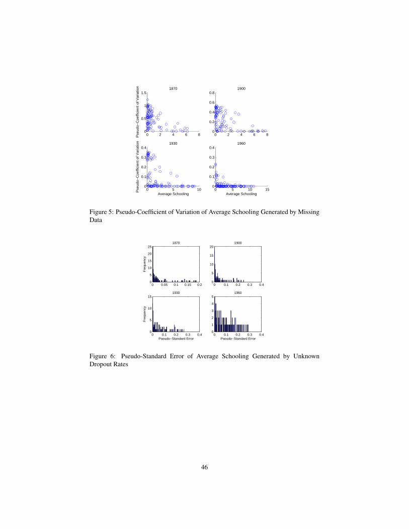
0 2 4 6 80
0.5
1
1.5
Pse
udo−
Coe
ffici
ent o
f Var
iatio
n 1870
0 2 4 6 80
0.2
0.4
0.6
0.81900
0 5 100
0.1
0.2
0.3
0.4
Pse
udo−
Coe
ffici
ent o
f Var
iatio
n
Average Schooling
1930
0 5 10 150
0.1
0.2
0.3
0.41960
Average Schooling
Figure 5: Pseudo-Coefficient of Variation of Average Schooling Generated by MissingData
0 0.05 0.1 0.15 0.20
5
10
15
20
25
Fre
quen
cy
1870
0 0.1 0.2 0.3 0.40
5
10
15
201900
0 0.1 0.2 0.3 0.40
5
10
15
Pseudo−Standard Error
Fre
quen
cy
1930
0 0.1 0.2 0.3 0.40
1
2
3
4
5
Pseudo−Standard Error
1960
Figure 6: Pseudo-Standard Error of Average Schooling Generated by UnknownDropout Rates
46

0 0.1 0.2 0.3 0.40
10
20
301870
Fre
quen
cy
−0.05 0 0.05 0.1 0.150
5
10
151900
−0.05 0 0.05 0.1 0.150
2
4
6
8
10
Pseudo−Standard Error
Fre
quen
cy
1930
−0.05 0 0.05 0.1 0.150
2
4
6
Pseudo−Standard Error
1960
Figure 7: Pseudo-Standard Error of Average Schooling Generated by Unknown Dura-tion of Primary
0 0.05 0.10
5
10
15
Fre
quen
cy
1870
0 0.1 0.2 0.3 0.40
2
4
6
8
101900
0 0.2 0.4 0.6 0.80
2
4
6
8
10
Pseudo−Standard Error
1930
Fre
quen
cy
0 0.5 10
2
4
6
8
Pseudo−Standard Error
1960
Figure 8: Pseudo-Standard Error of Average Schooling Generated by Unknown AgePyramid
47

0 2 4 6 8 10 120
2
4
6
8
10
12
Cohen−Soto
His
toric
al D
ata
Set
France Switzerland
Figure 9: Comparison of Average Years of Schooling in 1960
0 1 2 3 4 5 60
1
2
3
4
5
6
7
Cohen−Soto
His
toric
al D
ata
Set
Figure 10: Comparison of Average Years of Primary Schooling in 1960
48

0 1 2 3 4 50
0.5
1
1.5
2
2.5
3
3.5
4
4.5
5
Cohen−Soto
His
toric
al D
ata
Set
France
Canada
New−Zeland
Australia
Switzerland
US
Figure 11: Comparison of Average Years of Secondary Schooling in 1960
0 0.1 0.2 0.3 0.4 0.5 0.60
0.1
0.2
0.3
0.4
0.5
Cohen−Soto
His
toric
al D
ata
Set
US
Australia
New−Zeland
Canada
Figure 12: Comparison of Average Years of Higher Education in 1960
49

−2.5 −2 −1.5 −1 −0.5 0 0.5 1 1.5 2 2.5−1.5
−1
−0.5
0
0.5
1
1.5
Standard Normal Quantiles
Qua
ntile
s of
Mea
sure
men
t Err
or D
istr
ibut
ion
QQ Plot of Measurement Error versus Standard Normal
Figure 13: Quantiles of Measurement Error versus Quantiles of a Standard NormalDistribution
50

1860 1880 1900 1920 1940 1960 1980 20000
2
4
6
8
10
12
14
Ave
rage
Yea
rs o
f Sch
oolin
g
Western countries
MENA
Eastern Asia
Latin America
Japan
Sub−SaharanAfrica
SouthernEurope
India
Russia
Figure 14: Weighted-Average of Educational Attainment by Geographical Area
51

0 1 2 3 4 5 6 7−2
0
2
4
6
Sch
oolin
g V
aria
tion
1870
−19
10
Schooling 1870
0 1 2 3 4 5 6 7 80
2
4
6
Sch
oolin
g V
aria
tion
1910
−19
60
Schooling 1910
Figure 15: Schooling Variations 1870-1960
0 2 4 6 8 10 120
2
4
6
8
Sch
oolin
g V
aria
tion
1960
−20
00
Schooling 1960
0 2 4 6 8 10 12 140
2
4
6
Sch
oolin
g V
aria
tion
1980
−20
10
Schooling 1980
Figure 16: Schooling Variations 1960-2010
52