the “china shock”, exports and u.s. employment: a global ... · 4 due to trade, but comparing...

The “China Shock”, Exports and U.S. Employment:

A Global Input-Output Analysis*

by

Robert C. Feenstraa University of California, Davis

and NBER

Akira Sasaharab University of Idaho

August 18, 2017

Abstract

We quantify the impact on U.S. employment from imports and exports during 1995-2011, using the World Input-Output Database. We find that the growth in U.S. exports led to increased demand for 2 million jobs in manufacturing, 0.5 million in resource industries, and a remarkable 4.1 million jobs in services, totaling 6.6 million. Two-thirds of those service sectors jobs are due to the export of services themselves, whereas one-third is due to the intermediate demand from manufacturing and resource – or merchandise – exports, so the total labor demand gain due to merchandise exports was 3.7 million jobs. In comparison, U.S. merchandise imports from China led to reduced demand of 1.4 million jobs in manufacturing and 0.6 million in services (with small losses in resource industries), with total job losses of 2.0 million. It follows that the expansion in U.S. merchandise exports relative to imports from China over 1995-2011 created net demand for about 1.7 million jobs. Comparing the growth of U.S. merchandise exports to merchandise imports from all countries, we find a fall in net labor demand due to trade, but comparing the growth of total U.S. exports to total imports from all countries, then there is a rise in net labor demand because of the growth in service exports. Key words: China, exports, employment, services, global input-output table JEL codes: E16, F14, F60, O19

* The authors would like to thank Gordon H. Hanson, Richard Harris, Jeronimo Carballo, Sergey Nigai, and conference participants at the Creative Perspective on International Trade and Foreign Direct Investment: A Celebration to Honor Jim Markusen, held at the University of Colorado, Boulder. a Department of Economics, University of California, Davis, One Shields Avenue, Davis, CA 95616, [email protected] b College of Business and Economics, University of Idaho, Moscow, ID 83844, [email protected]

1

1. Introduction

Arguably among the most significant event in international trade in recent decades has

been the rapid rise in exports from China since its entry into the World Trade Organization

(WTO) in 2001, or the “China shock”. Even before that date China received the low, most-

favored-nation tariffs associated with WTO membership by a vote of the U.S. Congress each

year. But after China’s accession to the WTO, the reduction in the uncertainty associated with

that vote contributed importantly to the surge in exports to the United States. This argument is

made by Pierce and Schott (2016) and by Handley and Limão (2017).1 Pierce and Schott find

that the surge in Chinese exports to the United States coincides with a substantial decline in U.S.

manufacturing employment. Handley and Limão find that the welfare gain for consumers due to

this increase in Chinese imports is of the same order of magnitude as the U.S. gain from new

imported varieties in the preceding decade. These findings highlight the dual roles that Chinese

imports play for the United States: on the one hand, they create import competition and labor-

market dislocation; and on the other hand, they benefit U.S. consumers.2

The first of these roles is pursued in a series of papers by Autor, Dorn, and Hanson (2013,

2014, and with Song, 2015). They analyze the effect of rising Chinese import competition

between 1990 and 2007 on local U.S. labor markets, exploiting the geographic differences in

import exposure arising from initial differences in industry specialization. Rising import

exposure increases unemployment, lowers labor force participation, and reduces wages in local

labor markets. At the aggregate level, a conservative estimate is that the import surge account for

one-quarter of the decline in U.S. manufacturing employment. Most recently, in joint work with

1 See also the confirming empirical evidence in Feng, Li and Swenson (2017). 2 Amiti, Dai, Feenstra and Romalis (2017) argue that the consumer benefits in the United States are due more to China’s reduction in its own tariffs on intermediate inputs, which led to a drop in the price of exports to the U.S., rather than the reduction in the uncertainty of tariffs in the U.S.

2

Acemoglu and Price, these authors find that the import surge from China also contributes to the

unusually slow employment growth in the United States following the financial crisis and the

Great Recession (Acemoglu, Autor, Dorn, Hanson and Price, 2016).

While these papers by Autor, Dorn, Hanson and co-authors have explored the negative

impact of import competition from China on employment in the United States, some recent

articles highlight the role of China as an engine of world economic growth (e.g. Vianna, 2016;

IMF, 2017; World Bank, 2017). These articles speak to the second role played by China, in

bringing consumer benefits as well as benefits to workers in export-oriented industries. Feenstra,

Ma and Xu (2017) have examined the positive employment effects of U.S. exports using

techniques similar to those in Autor, Dorn, and Hanson (2013, 2015). Depending on the

estimation method, they find the employment in manufacturing industries grew by roughly the

same amount due to global exports as the decline in employment due to Chinese imports. This

result is perhaps not surprising given the magnitude of growth in U.S. exports as compared to

total imports and imports from China. Relative to GDP, U.S. exports rose by 10 percentage

points from 1995 to 2011, imports rose by 15 percentage points, and imports from China rose by

4 percentage points from a very low base; see Figure 1. So whether we focus on U.S. exports to

the world or on imports from China, the magnitude of changes over this period has been large

and the potential employments effects are correspondingly large.

In this paper, we quantify the employment impacts of U.S. imports and exports using a

global input-output analysis.3 Specifically, we use the World Input-Output Database (WIOD) of

Timmer et al. (2014, 2015). In section 2 we follow the method of Los, Timmer and de Vries

(2015, 2016), which focuses on the demand side of the labor market, to quantify the positive

3 Wang et al. (2017) extend the regression analysis of Autor, Dorn and Hanson (2013, 2015) by using input-output variables. Feenstra and Sasahara (2017) and Wood (2017) also rely on global input-output analysis.

3

impact from U.S. exports on employment. We find that the growth in exports led to demand for

2 million jobs in manufacturing, 0.5 million in resource industries, and a remarkable 4.1 million

jobs in services over 1995-2011, totaling 6.6 million. Two-thirds of those service sectors jobs are

due to the export of services themselves, whereas one-third is due to the intermediate demand

from the manufacturing and resource – or what we call merchandise – exports, so the total

demand gains from merchandise exports are 3.7 million jobs, with 1.9 million in manufacturing,

0.45 million in natural resource industries, and 1.3 million in services. That 1.9 million jobs in

manufacturing is much the same as the 1.9 million added jobs for an earlier 16 year period,

1991-2007, estimated by Feenstra, Ma and Xu (2017).

In section 3 we consider U.S. imports from China. In that case, we must specify the

added U.S. production that would occur if imports from China had not grown, and we consider

several possible assumptions along these lines. Our preferred estimates give reduced demand due

to U.S. imports from China of 1.4 million jobs in manufacturing, and another 1 million in

services (with small losses in resource industries), over 1995-2011. One-half of those job losses

in services are due to increased U.S. service imports, with the other half due to intermediate

demand from merchandise exports, so the total demand reduction due to merchandise (mainly

manufacturing) imports are 2.0 million jobs. The import estimates are very close to those from

Acemoglu, Autor, Dorn, Hanson and Price (2016), who find about 1.0 million jobs lost directly

in manufacturing and another 1.0 million jobs lost through throughout the economy through

input-output linkages, during the slightly shorter period 1999-2011. It follows that the expansion

in U.S. merchandise exports relative to imports from China over 1995-2011 led to net demand

for about 1.7 million jobs. Extending our analysis to compare the growth of U.S. merchandise

exports to merchandise imports from all countries in section 4, we find a fall in net labor demand

4

due to trade, but comparing the growth of total U.S. exports to total imports from all countries,

then there is a rise in net labor demand because of the growth in service exports.

There are two limitations of the global input-output analysis. First, as we have already

indicated, the employment effects are calculated from the demand side of the labor market,

without consideration of how the labor market will clear. This limitation could be addressed by

incorporating the global input-output tables into a computable model with frictional labor market

clearing (e.g. Caliendo, Dvorkin and Parro, 2015), but we do not attempt that here. Second, the

changes in exports or imports that are held fixed to compute their impact on employment are the

actual changes in these trade flows, and not the exogenous portion of these changes that result

from a specific cause. Autor, Dorn, and Hanson (2013, 2015), for example, use Chinese exports

to eight other countries to instrument for Chinese exports to the U.S. In section 5 we pursue a

similar approach of predicting the change in U.S. merchandise imports from China and total

exports that are due to exogenous factors, including tariff changes and demand shifts. We find

that nearly two-thirds of the employment impacts are explained by these factors. Conclusions are

given in section 6 and additional material is gathered in the Appendixes.

2. U.S. Exports and Employment

2.1 Structure of the Global Input-Output Table

We consider a N-country and S-sector case to match with the WIOD input-output table,

which has N = 41 countries including the rest of the world and S = 35 sectors. Let ( , ),( , )i r j sx

denote the value of intermediate goods produced in sector r of country i and used by sector s of

country j. Final good flows are also described in a similar manner: jrid ),,( indicates the value of

final good produced in sector r of country i and demanded in country j. The gross value of output

5

of sector r of country i, ,i ry , is computed as the sum of sales for intermediate and final use over

all purchasing sectors and countries:

, ( , ),( , ) ( , ),i r i r j s i r js j j

y x d . (1)

By dividing the intermediate good flows by the gross output in the destination sector of the

destination country, we find the input-output coefficients:

( , ),( , ) ( , ),( , ) ,/i r j s i r j s j sa x y ,

which are arranged in the matrix,

(1,1),(1,1) (1,1),(1,2) (1,1),( , )

(1,2),(1,1) (1,2),(1,2) (1,2),( , )

(2,1),(1,1) (2,1),(1,2) (2,1),( , )

( , ),(1,1) ( , ),(1,2) ( , ),( , )

N S

N S

N S

N S N S N S N S

a a a

a a a

a a a

a a a

A

.

With N countries and S sectors, the global input-output matrix A is )()( SNSN , and it

extends the Leontief (1936) matrix to include international linkages between countries.

Denote the final demand of country j buying from country i with the 1S vector ,i jd ,

( ,1),

( ,2),,

1( , ),

i j

i ji jt

Si S j

d

d

d

d

and

1,

2,

( ) 1

,

kk

kk

N S

N kk

d

dD

d

,

where D is the stacked vector of final demands over all countries. Likewise we denote the gross

output from country i as the 1S vector iy , and we stack these in the ( ) 1N S vector Y.

Then equation (1) is written alternatively as

6

1( ) Y I A D ,

where I denotes an identity matrix. The inverse 1)( AI can be expressed as a geometric

series: 10

( ) nn I A D A D . The first term D is the direct output absorbed as final goods,

the second term AD is the intermediate goods used to produce those final goods, including

imported intermediate goods, and the third term 2A D includes the additional intermediate goods

employed to produce the first round of intermediate goods AD , etc.

The ( ) 1N S vector of employment in each country and sector is obtained by

multiplying the gross outputs by the ratio of employment to gross output in each sector, denoted

by ( , )i s , with the )()( SNSN diagonal matrix Λ , to obtain:

1( ) L Λ I A D . (2)

We shall use the global input output table provided by WIOD (Timmer et al., 2014, 2015), which

differs by year, so we henceforth add the subscript t to all variables. It is worth stressing that (2)

holds identically in WIOD in all years, meaning that labor demand (on the right) equal supply

(on the left). In our calculations we will be investigating changes to demand, but without

imposing labor-market clearing.

2.2 Quantifying the Employment Effect of Export Expansion

In this section we employ the technique proposed by Los et al. (2015) to quantify the

employment effect of the growth in U.S. exports to the world. Since the first year of the WIOD

database is 1995, as the baseline the employment effect of export expansion is computed as:

1 1 11995, 1995,( ) ( )EX EX

t t t t t t t L Λ I A D Λ I A D , (3)

where 1995,EX

tD is the hypothetical final demand matrix defined as follows:

7

1,

2,

1995, , ,1995( ) 1

,

ktk

ktk

EXt US US US k

t k USN S

N ktk

d

d

Dd d

d

.

From this definition, exports from the U.S. to the rest of the world are kept at the 1995 level

,1995US i

i USd

while the U.S. domestic purchases from the U.S. final-good producers ,US UStd and

trade in other countries are allowed change over time as they did.

The first term on the right of (3) measures the actual employment, while the latter term is

the employment in a hypothetical world where U.S. exports stayed the same at the 1995 level.

The gap between the two is interpreted as the employment effect of export expansion. A positive

number means job creation while a negative number implies job destruction. Although this

measure takes final good exports in the final demand matrix tD into consideration, it does not

take intermediate good exports in the global input-output matrix tA into account. The next

measure also includes changes in the exports of intermediate goods:

2 1 11995, 1995, 1995,( ) ( )EX EX EX

t t t t t t t L Λ I A D Λ I A D ,

where, 1,1 1, 2 1, 1,

2,1 2, 2 2, 2,

1995, ,1 , 2 , ,1995 1995 1995( ) ( )

,1 , 2 , ,

US Nt t t t

US Nt t t t

EXt US US US US US N

tN S N S

N N N US N Nt t t t

A A A A

A A A A

AA A A A

A A A A

,

denotes the global input-output matrix where each of elements in the matrix is a SS sub-matrix

8

describing intermediate good flows from a country to another:

( ,1),( ,1) ( ,1),( ,2) ( ,1),( , )

( ,2),( ,1) ( ,2),( ,2) ( ,2),( , ),

( , ),( ,1) ( , ),( ,2) ( , ),( , )

i j i j i j St t t

i j i j i j Si j t t tt

S Si S j i S j i S j S

t t t

a a a

a a a

a a a

A

,

which is a matrix of Leontief coefficients ( , ),( , )i r j sta denoting the intermediate good flows from

sector r of country i to sector s of country j in year t. But for the U.S. sub-matrices, ,1995{ }US k

k USA ,

the intermediate good flows from 1995 are employed to find the coefficients.

11995,EX

tL and 21995,EX

tL are both stacked 1)( SN vector of the employment effects over all

sectors and countries, and in either case we are particularly interested in the 1S sub-vector for

the U.S., ,1995,EX US

tL . Using the sectors available in WIOD, we aggregate the U.S. employment

effects into the natural resource sector (i.e. agricultural and mining, WIOD sectors 1-3),

manufacturing (sectors 4-16), and services (sectors 17-35), as follows:4

3,1995, 1995,1

( ) ( )EX US EX,USt ts

L Resource L s

,

16,1995, 1995,4


L Manufacturing L s

, (4)

35,1995, 1995,17


L Services L s

.

The overall employment effect in the U.S. economy is

35,1995, 1995,1


L All sectors L s

(5)

The same aggregation as (4)-(5) applied to the rest of the employment effect measures

presented in this paper.

4 See Appendix A for the list of the WIOD sectors.

9

The results from estimating the employment effect of export expansion are shown in

Table 1. Final good exports added demand for 760 thousand manufacturing jobs over 1995-2011,

which is 4.5% of total manufacturing employment in 1995. By taking intermediate exports into

account, the employment effect of export expansion becomes even greater – export expansion

added demand for 2.0 million manufacturing jobs, and another 0.5 million jobs in resource

industries. These estimates are only slightly larger than found for another 16 year period by

Feenstra, Ma and Xu (2017, note 9), who find gains in manufacturing jobs of 1.9 million due to

rising U.S. exports over 1991-2011. Still, considering that our input-output analysis is purely on

the demand side, whereas Feenstra, Ma and Xu are using equilibrium changes in employment,

and that we have not yet attempted to isolate exogenous changes in exports, there is surprising

similarity between the two sets of estimates. The extent of demand creation due to U.S. exports

is the greatest for the service sector, where final good exports added 0.9 million jobs while

intermediate exports added another extra 3.2 million jobs– 4.1 million in total.

These total estimates for the three sectors are carried over into column (1) of Table 2.

There we separate the direct plus indirect effects of manufacturing and resource exports – or

what we call merchandise exports – from the direct plus indirect effect of service exports. We

see that for the merchandise sectors, nearly the entire added labor demand is due to the exports of

these industries themselves. But for the service sector, comparing columns (2) and (3) of Table 2,

we find one-third of the job gains arise indirectly due to manufacturing and resource exports,

whereas two-thirds of these job gains are explained by exports of final or intermediate services

themselves. Our focus in this paper shall be on the exports of manufacturing and resource

industries, including its intermediate demand for service jobs. From column (2), then, we see that

U.S. exports led to increased demand of about 1.9 million manufacturing jobs, 0.45 resource

10

industry jobs and 1.3 service sector jobs, or 3.7 million jobs in total during 1995-2011. These

results show that U.S. labor demand has grown substantially from export opportunities.

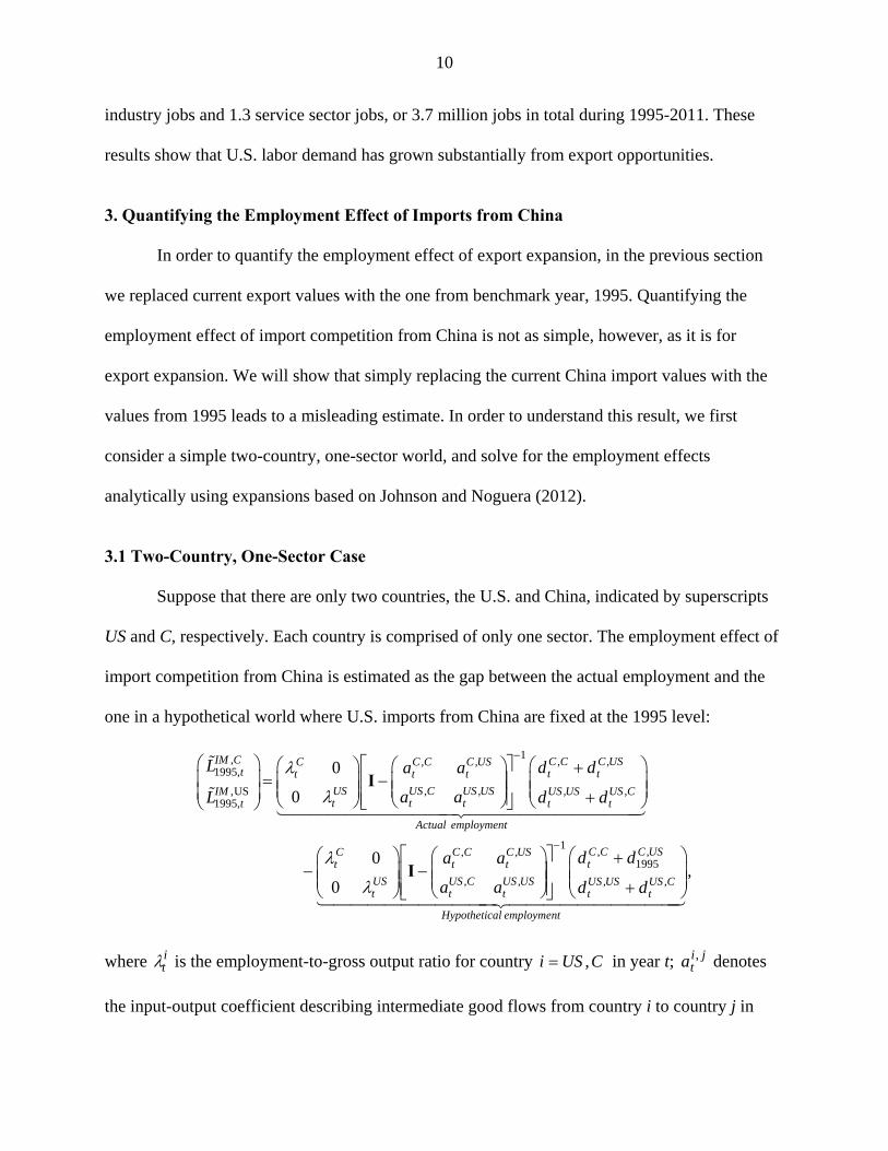
3. Quantifying the Employment Effect of Imports from China

In order to quantify the employment effect of export expansion, in the previous section

we replaced current export values with the one from benchmark year, 1995. Quantifying the

employment effect of import competition from China is not as simple, however, as it is for

export expansion. We will show that simply replacing the current China import values with the

values from 1995 leads to a misleading estimate. In order to understand this result, we first

consider a simple two-country, one-sector world, and solve for the employment effects

analytically using expansions based on Johnson and Noguera (2012).

3.1 Two-Country, One-Sector Case

Suppose that there are only two countries, the U.S. and China, indicated by superscripts

US and C, respectively. Each country is comprised of only one sector. The employment effect of

import competition from China is estimated as the gap between the actual employment and the

one in a hypothetical world where U.S. imports from China are fixed at the 1995 level:

1, , ,, ,1995,

, ,,US , ,1995,

, ,

0

0

0

0

IM C C C C USC C C C USt t tt t t

US US C US USIM US US US Ct t tt t t

Actual employment

C C C C USt t t

USt

L d da a

a aL d d

a a

a

I

I

1, ,

1995

, , , ,,

C C C USt

US C US US US US US Ct t t t

Hypothetical employment

d d

a d d

where it is the employment-to-gross output ratio for country CUSi , in year t; ,i j

ta denotes

the input-output coefficient describing intermediate good flows from country i to country j in

11

year t; and ,i jtd denotes final good flows from country i to country j in year t.

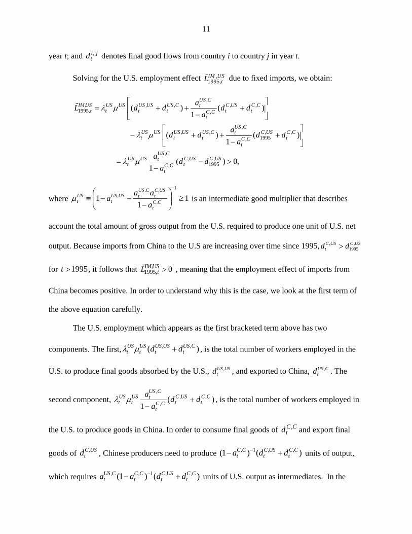
Solving for the U.S. employment effect ,1995,IM US

tL due to fixed imports, we obtain:

,, , , ,

1995, ,

,, , , ,

1995,

,, ,

1995,

( ) ( )1

( ) ( )1

( ) 0,1

US CIM,US US US US US US C C US C Ct

t t t t t tC Ct

US CUS US US US US C C US C Ctt t t tC C

t

US CUS US C US C UStt tC C

t

aL d d d d

a

ad d d d

a

ad d

a

where 11

1

1

,

,,,

CCt

USCt

CUStUSUS

tUSt a

aaa is an intermediate good multiplier that describes

account the total amount of gross output from the U.S. required to produce one unit of U.S. net

output. Because imports from China to the U.S are increasing over time since 1995, USCUSCt dd ,

1995,

for 1995t , it follows that 1995, 0IM,UStL , meaning that the employment effect of imports from

China becomes positive. In order to understand why this is the case, we look at the first term of

the above equation carefully.

The U.S. employment which appears as the first bracketed term above has two

components. The first, , ,( )US US US US US Ct t t td d , is the total number of workers employed in the

U.S. to produce final goods absorbed by the U.S., USUStd , , and exported to China, CUS

td , . The

second component, ,

, ,,

( )1

US CUS US C US C Ctt t t tC C

t

ad d

a

, is the total number of workers employed in

the U.S. to produce goods in China. In order to consume final goods of ,C Ctd and export final

goods of ,C UStd , Chinese producers need to produce , 1 , ,(1 ) ( )C C C US C C

t t ta d d units of output,

which requires , , 1 , ,(1 ) ( )US C C C C US C Ct t t ta a d d units of U.S. output as intermediates. In the

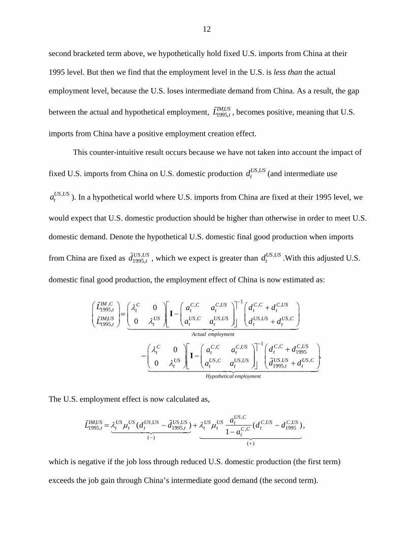
12

second bracketed term above, we hypothetically hold fixed U.S. imports from China at their

1995 level. But then we find that the employment level in the U.S. is less than the actual

employment level, because the U.S. loses intermediate demand from China. As a result, the gap

between the actual and hypothetical employment, 1995,IM,US

tL , becomes positive, meaning that U.S.

imports from China have a positive employment creation effect.

This counter-intuitive result occurs because we have not taken into account the impact of

fixed U.S. imports from China on U.S. domestic production ,US UStd (and intermediate use

,US USta ). In a hypothetical world where U.S. imports from China are fixed at their 1995 level, we

would expect that U.S. domestic production should be higher than otherwise in order to meet U.S.

domestic demand. Denote the hypothetical U.S. domestic final good production when imports

from China are fixed as ,1995,US US

td , which we expect is greater than ,US UStd .With this adjusted U.S.

domestic final good production, the employment effect of China is now estimated as:

1, , ,, ,1995,

, , , ,1995,

, ,

0

0

0

0

IM C C C C USC C C C USt t tt t t

US US C US USIM,US US US US Ct t tt t t

Actual employment

C C C C USt t t

USt

L d da a

a aL d d

a a

a

I

I

1 , ,1995

, ,, ,1995,

.C C C USt

US US US CUS C US USt tt t

Hypothetical employment

d d

d da

The U.S. employment effect is now calculated as,

,, , , ,

1995, 1995, 1995,

( )( )

( ) ( ) ,1

US CIM,US US US US US US US US US C US C USt

t t t t t t t tC Ct

aL d d d d

a

which is negative if the job loss through reduced U.S. domestic production (the first term)

exceeds the job gain through China’s intermediate good demand (the second term).

13

This simple two-country and one-sector example shows that simply replacing imports

from China to the U.S. with the one from benchmark year does not lead to a reasonable result,

because U.S. domestic production also needs to be adjusted. In Appendix B, we confirm that this

counter-intuitive result holds quantitatively in the multi-country, multi-sector WIOD model. In

the following section, we consider the general case and propose ways to find hypothetical U.S.

domestic production when imports from China stay at the benchmark year level.

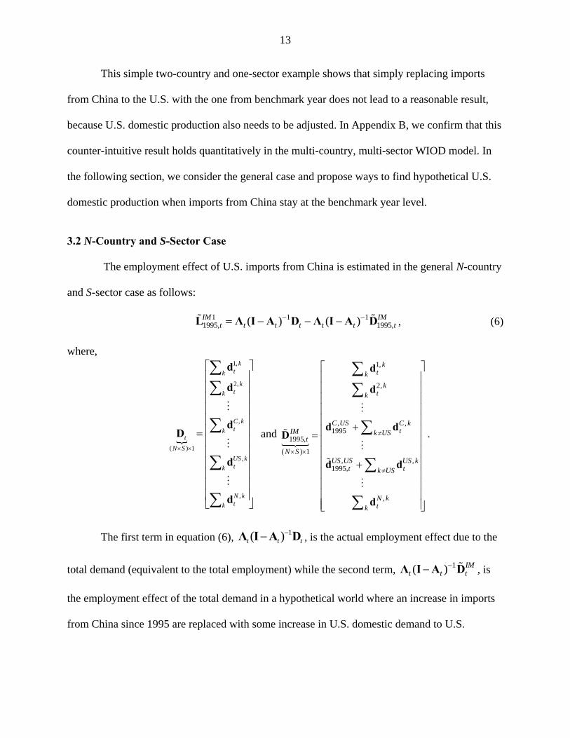
3.2 N-Country and S-Sector Case

The employment effect of U.S. imports from China is estimated in the general N-country

and S-sector case as follows:

1 1 11995, 1995,( ) ( )IM IM


where,

k

kNt

k

kUSt

k

kCt

k

kt

k

kt

SN

t

,

,

,

,2

,1

1)(

d

d

d

d

d

D

and

1,

2,

, ,1995

1995,

( ) 1, ,

1995,

,

ktk

ktk

C US C ktIM k US

t

N SUS US US k

t tk US

N ktk

d

d

d dD

d d

d

.

The first term in equation (6), ttt DAIΛ 1)( , is the actual employment effect due to the

total demand (equivalent to the total employment) while the second term, 1( ) IMt t t

Λ I A D , is

the employment effect of the total demand in a hypothetical world where an increase in imports

from China since 1995 are replaced with some increase in U.S. domestic demand to U.S.

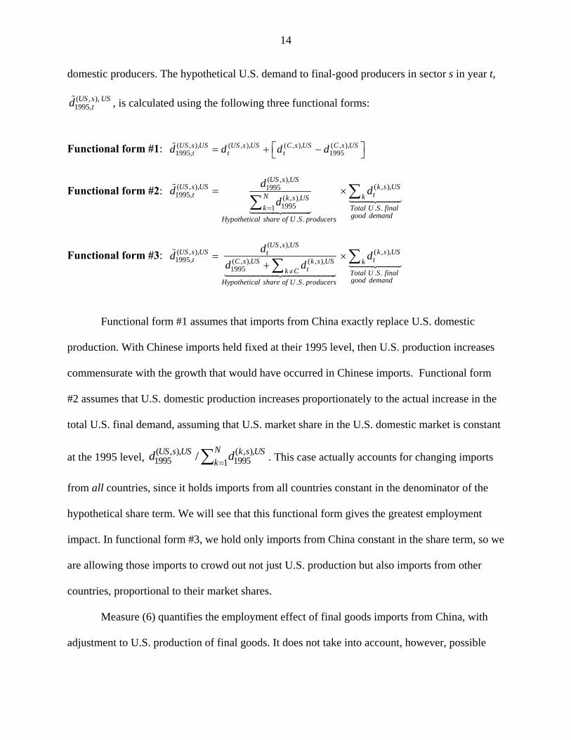
14

domestic producers. The hypothetical U.S. demand to final-good producers in sector s in year t,

( , ),1995,

US s UStd , is calculated using the following three functional forms:

Functional form #1: ( , ), ( , ), ( , ), ( , ),1995, 1995

US s US US s US C s US C s USt t td d d d

Functional form #2: ( , ),

( , ), ( , ),19951995, ( , ),

19951 . .

. .

US s USUS s US k s US

t tN kk s USk Total U S final

good demandHypothetical share of U S producers

dd d

d

Functional form #3: ( , ),

( , ), ( , ),1995, ( , ), ( , ),

1995 . .. .

US s USUS s US k s USt

t tC s US k s US ktk C Total U S final


dd d

d d

Functional form #1 assumes that imports from China exactly replace U.S. domestic

production. With Chinese imports held fixed at their 1995 level, then U.S. production increases

commensurate with the growth that would have occurred in Chinese imports. Functional form

#2 assumes that U.S. domestic production increases proportionately to the actual increase in the

total U.S. final demand, assuming that U.S. market share in the U.S. domestic market is constant

at the 1995 level, ( , ), ( , ),1995 19951

/NUS s US k s USk

d d . This case actually accounts for changing imports

from all countries, since it holds imports from all countries constant in the denominator of the

hypothetical share term. We will see that this functional form gives the greatest employment

impact. In functional form #3, we hold only imports from China constant in the share term, so we

are allowing those imports to crowd out not just U.S. production but also imports from other

countries, proportional to their market shares.

Measure (6) quantifies the employment effect of final goods imports from China, with

adjustment to U.S. production of final goods. It does not take into account, however, possible

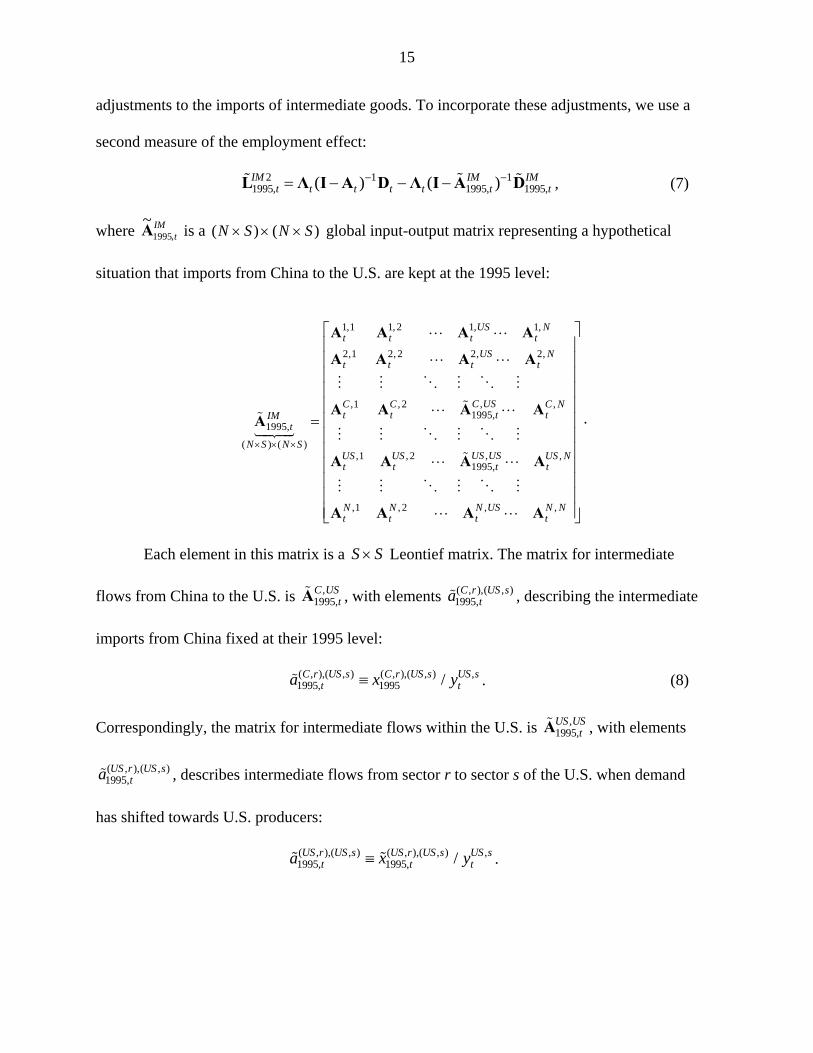
15

adjustments to the imports of intermediate goods. To incorporate these adjustments, we use a

second measure of the employment effect:

2 1 11995, 1995, 1995,( ) ( )IM IM IM


where IMt,1995

~A is a )()( SNSN global input-output matrix representing a hypothetical

situation that imports from China to the U.S. are kept at the 1995 level:

1,1 1, 2 1, 1,

2,1 2, 2 2, 2,

,,1 , 2 ,1995,

1995,

( ) ( ),,1 , 2 ,

1995,

,1 , 2 , ,

US Nt t t t

US Nt t t t

C USC C C Nt t t tIM

t

N S N SUS USUS US US N

t t t t

N N N US N Nt t t t

A A A A

A A A A

A A A AA

A A A A

A A A A

.

Each element in this matrix is a SS Leontief matrix. The matrix for intermediate

flows from China to the U.S. is ,1995,C US

tA , with elements ( , ),( , )1995,

C r US sta , describing the intermediate

imports from China fixed at their 1995 level:

( , ),( , ) ( , ),( , ) ,1995, 1995 /C r US s C r US s US s

t ta x y . (8)

Correspondingly, the matrix for intermediate flows within the U.S. is ,1995,US US

tA , with elements

( , ),( , )1995,US r US s

ta , describes intermediate flows from sector r to sector s of the U.S. when demand

has shifted towards U.S. producers:

( , ),( , ) ( , ),( , ) ,1995, 1995, /US r US s US r US s US s

t t ta x y .

16

The intermediates value ( , ),( , )1995,US r US s

tx sold from sector r to sector s of the U.S. are calculated

using the same three functional forms as used for final goods:

Functional form #1: ( , ),( , ) ( , ),( , ) ( , ),( , ) ( , ),( , )1995, 1995US r US s US r US s C r US s US r US s

t t tx x x x

Functional form #2: ( , ),( , )

( , ),( , ) ( , ),( , )19951995, ( , ),( , )

19951 . .

. .

US r US sUS r US s k r US s

t tN kk r US sk Total U S intermediate


xx x

x

Functional form #3: ( , ),( , )

( , ),( , ) ( , ),( , )1995, ( , ),( , ) ( , ),( , )

1995. .

. .

US r US sUS r US s k r US st

t tC r US s k r US s ktk C Total U S intermediate


xx x

x x

Table 3 summarizes the employment effect of imports from China estimated by adjusting

the U.S. domestic production using the three functional forms above. Panels A through C show

the result from using functional forms #1 through #3, respectively. Panel A shows that final good

imports from China led to reduced labor demand of 0.8 million jobs in manufacturing, 40

thousand jobs in resource industries, and 350 thousand service sector jobs, or 1.2 million jobs in

total. Together with intermediate goods imports from China, reduced U.S. labor demand become

1.4 million, 60 thousand, and 960 thousand in the manufacturing, resource, and the service sector,

respectively, or 2.4 million jobs in total.

Panel B reports the result from using functional form #2. It predicts a greater negative

employment impact in the manufacturing and the resource sectors. Final good and intermediate

imports from China reduce demand for manufacturing jobs by 2.9 million and resource jobs by

0.5 million. Together with 2.5 million service sector jobs lost, the overall job losses add up to 5.9

million. Functional form #3 leads to the smallest demand reduction as shown in Panel C. Imports

of final goods and intermediate goods from China led to 0.7 million job losses in manufacturing,

17

40 thousand job losses in resource industries, and another 0.7 million job losses in services, for

overall reduced demand of 1.4 million jobs.

Our results are evidently sensitive to the assumed functional form for the implied U.S.

domestic production. In the next section, we utilize the actual data to relate the market share of

U.S. domestic producers to imports from China in regression framework, and propose a fourth

estimate of the employment effect of these imports.

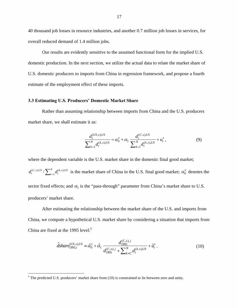
3.3 Estimating U.S. Producers’ Domestic Market Share

Rather than assuming relationship between imports from China and the U.S. producers

market share, we shall estimate it as:

( , ), ( , ),

0 1( , ), ( , ),1 1

US s US C s USs st t

tN Nk s US k s USt tk k

d du

d d

, (9)

where the dependent variable is the U.S. market share in the domestic final good market;

N

k

USskt

USsCt dd

1

),,(),,( / is the market share of China in the U.S. final good market; 0s denotes the

sector fixed effects; and 1 is the “pass-through” parameter from China’s market share to U.S.

producers’ market share.

After estimating the relationship between the market share of the U.S. and imports from

China, we compute a hypothetical U.S. market share by considering a situation that imports from

China are fixed at the 1995 level:5

( , ),( , ), 19951995, 0 1 ( , ), ( , ),

1995

ˆ ˆ ˆ ˆC s j

US s US s st tNC s j k s US

tk C

ddshare u

d d

. (10)

5 The predicted U.S. producers’ market share from (10) is constrained to lie between zero and unity.

18

Using this estimated U.S. share and the actual total U.S. final good demand

N

k

USsktd

1

),,( , we

compute the hypothetical U.S. domestic production as:

( , ), ( , ), ( , ),1995, 1995, 1

ˆ ˆ NUS s US US s US k s USt t tk

d dshare d

. (11)

Similarly, in order to find a relationship between U.S. producers’ market share in the U.S.

domestic intermediate good market and intermediate imports from China, we estimate:

( , ),( , ) ( , ),( , ), ,

0 1( , ),( , ) ( , ),( , )1 1

US r US s C r US sr s s r st t

tN Nk r US s k r US st tk k

x xu

x x

, (12)

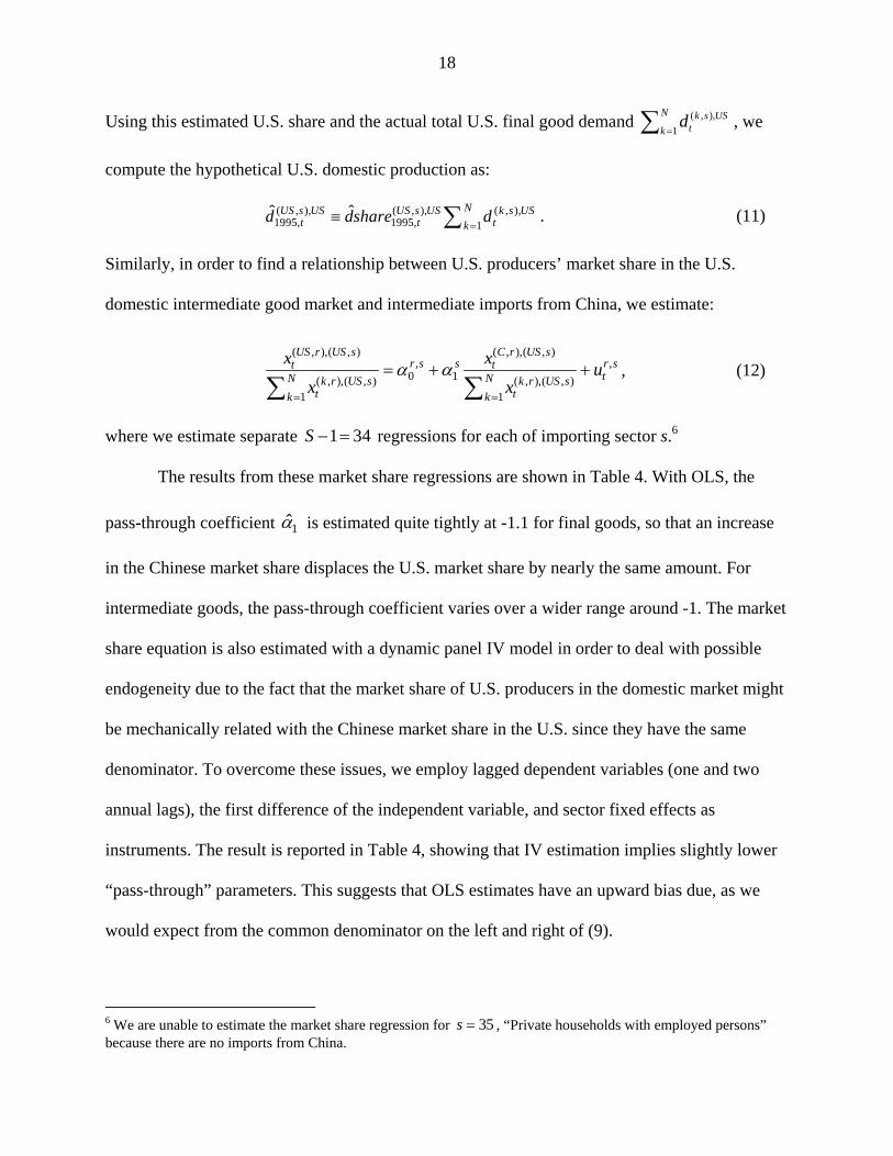
where we estimate separate 341S regressions for each of importing sector s.6

The results from these market share regressions are shown in Table 4. With OLS, the

pass-through coefficient 1̂ is estimated quite tightly at -1.1 for final goods, so that an increase

in the Chinese market share displaces the U.S. market share by nearly the same amount. For

intermediate goods, the pass-through coefficient varies over a wider range around -1. The market

share equation is also estimated with a dynamic panel IV model in order to deal with possible

endogeneity due to the fact that the market share of U.S. producers in the domestic market might

be mechanically related with the Chinese market share in the U.S. since they have the same

denominator. To overcome these issues, we employ lagged dependent variables (one and two

annual lags), the first difference of the independent variable, and sector fixed effects as

instruments. The result is reported in Table 4, showing that IV estimation implies slightly lower

“pass-through” parameters. This suggests that OLS estimates have an upward bias due, as we

would expect from the common denominator on the left and right of (9).

6 We are unable to estimate the market share regression for 35s , “Private households with employed persons” because there are no imports from China.

19

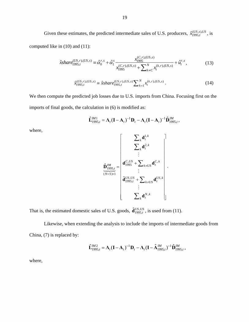
Given these estimates, the predicted intermediate sales of U.S. producers, ( , ),1995,ˆ US s US

tx , is

computed like in (10) and (11):

( , ),( , )( , ),( , ) , ,19951995, 0 1 ( , ),( , ) ( , ),( , )

1995

ˆ ˆˆ ˆC r US s

US r US s r s s r st tNC r US s k r US s

tk C

xxshare u

x x

, (13)

( , ),( , ) ( , ),( , ) ( , ),( , )1995, 1995, 1

ˆ ˆNUS r US s US r US s k r US s

t t tkx xshare x

. (14)

We then compute the predicted job losses due to U.S. imports from China. Focusing first on the

imports of final goods, the calculation in (6) is modified as:

1 1 11995, 1995,

ˆ ˆ( ) ( )IM IMt t t t t t t

L Λ I A D Λ I A D ,

where, 1,

2,

, ,1995

1995,

( ) 1, ,

1995,

,

ˆ

ˆ

ktk

ktk

C US C ktIM k US

t

N SUS US US k

t tk US

N ktk

d

d

d dD

d d

d

.

That is, the estimated domestic sales of U.S. goods, ,1995,

ˆUS UStd , is used from (11).

Likewise, when extending the analysis to include the imports of intermediate goods from

China, (7) is replaced by:

2 1 11995, 1995, 1995,

ˆˆ ˆ( ) ( )IM IM IMt t t t t t t


where,

20

1,1 1, 2 1, 1,

2,1 2, 2 2, 2,

,,1 , 2 ,1995,

1995,

( ) ( ),,1 , 2 ,

1995,

,1 , 2 , ,

ˆ

US Nt t t t

US Nt t t t

C USC C C Nt t t tIM

t

N S N SUS USUS US US N

t t t t

N N N US N Nt t t t

A A A A

A A A A

A A A AA

A A A A

A A A A

.

The input-output coefficients for China’s sales to the U.S., ,1995,C US

tA , are still calculated by holding

Chinese imports fixed at their 1995 levels, as in (8). But the input-output coefficients for the U.S.

are computed using the predicted U.S. sales,

( , ),( , ) ( , ),( , ) ,1995, 1995,ˆ ˆ /US r US s US r US s US s

t t ta x y .

The results from using predicted U.S. final and intermediate sales based on the OLS

estimates are shown in Table 5a. In column (1), we report the estimated reduction in labor

demand from all final good and intermediate imports from China. These are 1.4 million in

manufacturing, 55 thousand in resource industries, and 1.1 million in services, for a total of 2.6

million. Within the job losses in services, about one-half (560 thousand) are due to input-output

linkages with the merchandise imports (i.e. manufacturing and resource imports), and the other

one-half (500 thousand) are due to competition from direct service imports. The results based on

the IV estimates are summarized in Table 5b. Because the IV estimation leads to slightly smaller

“pass-through” parameters, the implied negative employment effect of China is somewhat

smaller than in Table 5a. It shows that there is reduced demand for 1.25 million manufacturing

jobs, 50 thousand in natural resource sectors, and 900 thousand in services, totaling for 2.2

million job losses are due to import penetration from China in the U.S.

21

Focusing on the merchandise sector and its intermediate demand into services, column

(2) shows overall job losses of 1.8-2.0 million (the former is based on IV while the latter is based

on OLS). This estimate is very close to Acemoglu, Autor, Dorn, Hanson, and Price (2016), who

find that import competition from China led to about 1.0 million job losses in manufacturing and

another 1.0 million job losses through input-output linkages with the rest of the economy, during

the slightly shorter period 1999-2011.

4. Net Employment Effects

We now compare more carefully the positive impact of U.S. exports on labor demand to

the negative effect from imports, reporting the net impact on jobs. Table 6 summarizes our

results for U.S. total exports and imports from China over 1995-2011. Panel A provides the net

employment effect from trade in the merchandise sectors, including their indirect effect on

services, while panel B provides the net effects from trade in all sectors. For merchandise exports

and imports from China, we have found added demand of 3.7 million jobs and reduced demand

of 2.0 million jobs, respectively, giving a net gain of 1.7 million jobs. That number is the final

entry in column (3) of panel A, which uses the estimates from our OLS market share regressions.

Alternatively, for trade in all sectors, we obtain a much larger net gain of 4.0 million jobs, the

final entry in panel B, and that is because of the growth in U.S. service exports. The last column

is based on our IV market share regressions, showing that merchandise trade led to demand for

0.73 million net jobs and trade in all sectors added demand for 4.4 million jobs.

In Table 6 we also include the net employment estimates obtained while using differing

assumptions on the response of U.S. production to imports from China. Functional form #1

assumes that Chinese imports displace U.S. production dollar-for-dollar, and it gives results

similar to the market share regressions, i.e. net job gains of 1.8 million and 4.2 million for

22

merchandise trade and total trade, respectively. Somewhat larger estimates of net gains are

obtained from functional form #3. We do not report in Table 6 the results for functional form #2

because, as we have already noted, that specification really allows for U.S. production to be

responding to the imports of all countries.

In Table 7, we extend our earlier analysis to report results for U.S. total exports net of

imports from all countries over 1995-2011. For merchandise trade, we obtain a net reduction in

labor demand: for the three functional forms for the possible displacement of U.S. production,

we obtain net job losses ranging from -3.3 to -0.5 million at the bottom of panel A.7 We are not

able to implement the market share regressions in this case because, for some trading partners,

that regression is too unstable. So we simply conclude that there is a negative net impact on U.S.

labor demand from merchandise trade, without being more precise about its magnitude. When

we take into account trade in all sectors, however, in panel B, then the net impact on labor

demand becomes positive 0.7 million jobs for functional forms #2 and #3, though it is still

negative for functional form #1. We find the dollar-for-dollar displacement of U.S. producers,

assumed in functional form #1, to be rather implausible and so we have more confidence in the

results from the other two specifications. In these cases, the positive net impact of trade on labor

demand is explained by the growth in U.S. service exports.8

5. Decomposing the Employment Effects

5.1 Decomposing the Employment Effect of Export Expansion

7 In functional form #1, we increase U.S. production dollar-for-dollar for the difference over all countries between their imports each year and in 1995. Similarly, for functional form #3 we hold the U.S. imports from all countries fixed at their 1995 value when calculating the hypothetical share of U.S. producers. 8 See the 2.8 million service sector jobs created by those exports in Table 2.

23

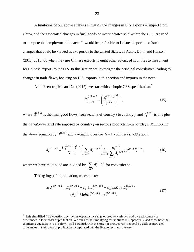
A limitation of our above analysis is that all the changes in U.S. exports or import from

China, and the associated changes in final goods or intermediates sold within the U.S., are used

to compute that employment impacts. It would be preferable to isolate the portion of such

changes that could be viewed as exogenous to the United States, as Autor, Dorn, and Hanson

(2013, 2015) do when they use Chinese exports to eight other advanced countries to instrument

for Chinese exports to the U.S. In this section we investigate the principal contributors leading to

changes in trade flows, focusing on U.S. exports in this section and imports in the next.

As in Feenstra, Ma and Xu (2017), we start with a simple CES specification:9

1( , ), ( , ),

( , ), ( , ),

US s j US s jt t

i s j i s jt t

d

d

, (15)

where jsitd ),,( is the final good flows from sector s of country i to country j, and jsi

t),,( is one plus

the ad valorem tariff rate imposed by country j on sector s products from country i. Multiplying

the above equation by ( , ),i s jtd and averaging over the 1N countries i US yields:

( , ), 1 ( , ),( , ), ( , ), ( , ), 1

( , ),

( )( )

1

US s j i s jUS s j k s j i s jt t

t t tk s jk US i US t

k US

dd d

N d

, (16)

where we have multiplied and divided by ( , ),k s jt

k US

d for convenience.

Taking logs of this equation, we estimate:

( , ),( , ), ( , ), ( , ),1 20

( , ), ( , ),3

ln ln ln

ln ,

US s jUS s j US s j US s jt t t

US s j US s jt t

d MultiD

Multi

(17)

9 This simplified CES equation does not incorporate the range of product varieties sold by each country or differences in their costs of production. We relax these simplifying assumptions in Appendix C, and show how the estimating equation in (16) below is still obtained, with the range of product varieties sold by each country and differences in their costs of production incorporated into the fixed effects and the error.

24

where ( , ),0US s j is a destination-sector fixed effect and the variable ( , ),US s j

tMultiD is a

“multilateral demand” term defined as,

( , ), ( , ),US s j k s jt tk US

MultiD d

, (18)

which is the sum of final good flows from all countries besides the U.S. to country j. The final

variable, jsitMulti ),,( denotes the “multilateral tariffs” applied by country j to trading partners

other than the U.S:

( , ), ( , ), 1( , ),

( , ),

( )i s j i s jt tUS s j i US

t k s jtk US

dMulti

d

, (19)

where is the elasticity of substitution.10 Comparing (16) and (17) we see that the monopolistic

competition model implies that 1 ( 1) , and 2 3 1 .

We treat the variables in (18) and (19) as exogenous to the error term in (17), and use

these variables to predict the trade flows due to each of these instruments. Specifically, after

estimating (17), we compute the hypothetical final good flows from the U.S. to the rest of the

world when the tariff rates imposed on U.S. exporters remain at the 1995 level as:

1995

( , ), ( , ),( , ), ( , ),1 20 1995

( , ), ( , ),3

ˆ ˆ ˆ ˆln ln ln

ˆ ˆln .

US s j US s jUS s j US s jt t

US s j US s jt t

d MultiD

Multi

(20)

Note that the tariff variable used to calculate this predicted demand is replaced with its 1995

value, ( , ),1995US s j , and we include the estimated residual in (20) so that we will be able to

determine what amount of the employment effects are due to this unexplained portion.11 We

10 The estimates we obtain for 1 are as large as -5, implying = 6, and we shall impose that value when

constructing the multilateral tariff term in (19). 11 Note that with the difference between actual and estimated final demand used in (21), including the residual in (20) ensures that only the difference between the 1995 and actual tariffs drives the result.

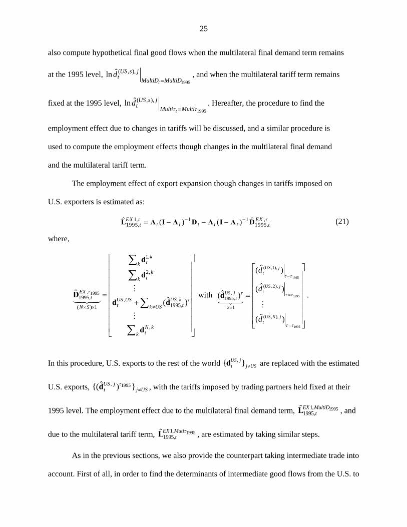
25

also compute hypothetical final good flows when the multilateral final demand term remains

at the 1995 level, 1995

( , ),ˆlnt

US s jt

MultiD MultiDd

, and when the multilateral tariff term remains

fixed at the 1995 level, 1995

( , ),ˆlnt

US s jt

Multi Multid

. Hereafter, the procedure to find the

employment effect due to changes in tariffs will be discussed, and a similar procedure is

used to compute the employment effects though changes in the multilateral final demand

and the multilateral tariff term.

The employment effect of export expansion though changes in tariffs imposed on

U.S. exporters is estimated as:

1, 1 1 ,1995, 1995,

ˆ ˆ( ) ( )EX EXt t t t tt t

L Λ I A D Λ I A D (21)

where,

1995

1,

2,

,1995, ,,

1995,( ) 1

,

ˆˆ( )

ktk

ktk

EXt US kUS US

t tk USN S

N ktk

d

d

Dd d

d

with

1995

1995

1995

)ˆ(

)ˆ(

)ˆ(

)ˆ(

),,(

),2,(

),1,(

1

,,1995

jSUSt

jUSt

jUSt

S

jUSt

d

d

d

d .

In this procedure, U.S. exports to the rest of the world USj

jUSt }{ ,d are replaced with the estimated

U.S. exports, 1995,ˆ{( ) }US jt j US

d , with the tariffs imposed by trading partners held fixed at their

1995 level. The employment effect due to the multilateral final demand term, 19951,1995,

ˆEX MultiDtL , and

due to the multilateral tariff term, 19951,1995,

ˆEX Mutit

L , are estimated by taking similar steps.

As in the previous sections, we also provide the counterpart taking intermediate trade into

account. First of all, in order to find the determinants of intermediate good flows from the U.S. to

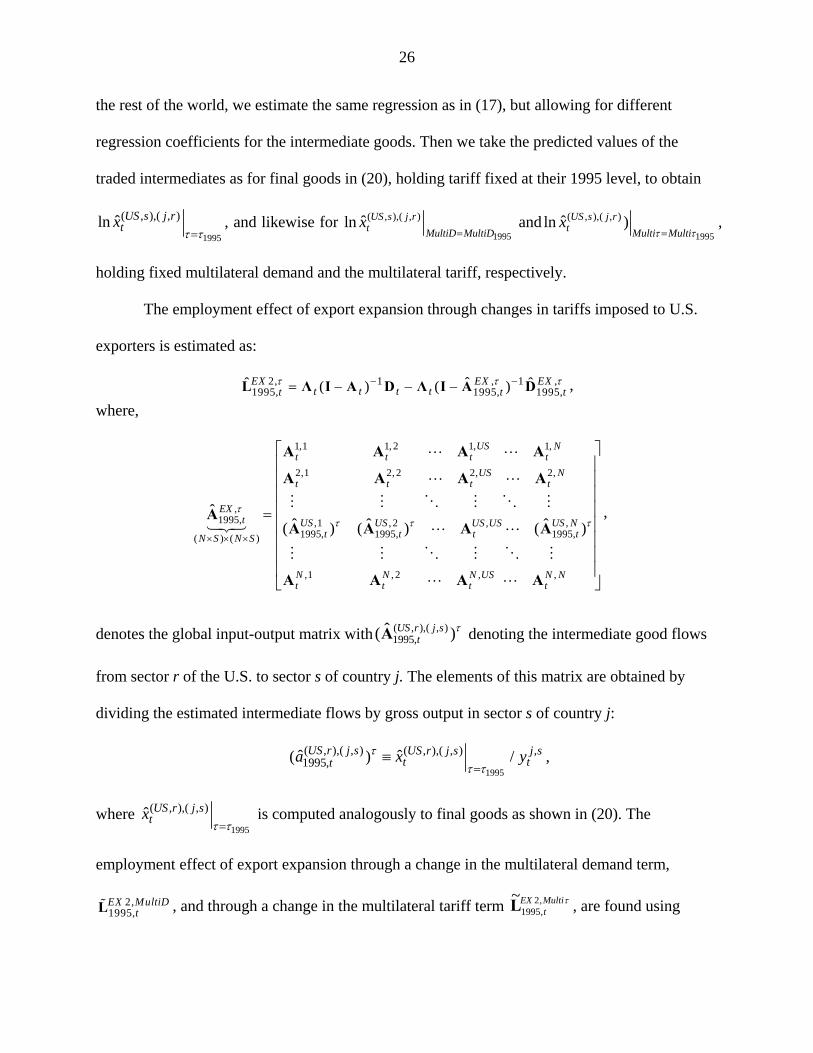
26

the rest of the world, we estimate the same regression as in (17), but allowing for different

regression coefficients for the intermediate goods. Then we take the predicted values of the

traded intermediates as for final goods in (20), holding tariff fixed at their 1995 level, to obtain

1995

( , ),( , )ˆln US s j rtx

, and likewise for

1995

( , ),( , )ˆln US s j rt MultiD MultiD

x

and1995

( , ),( , )ˆln )US s j rt Multi Multi

x

,

holding fixed multilateral demand and the multilateral tariff, respectively.

The employment effect of export expansion through changes in tariffs imposed to U.S.

exporters is estimated as:

2, 1 , 1 ,1995, 1995, 1995,

ˆˆ ˆ( ) ( )EX EX EXt t t tt t t


where,

1,1 1, 2 1, 1,

2,1 2, 2 2, 2,

,1995, ,1 , 2 ,,

1995, 1995, 1995,( ) ( )

,1 , 2 , ,

ˆˆ ˆ ˆ( ) ( ) ( )

US Nt t t t

US Nt t t t

EXt US US US NUS US

t t t tN S N S

N N N US N Nt t t t

A A A A

A A A A

AA A Α A

A A A A

,

denotes the global input-output matrix with ( , ),( , )1995,

ˆ( )US r j st

A denoting the intermediate good flows

from sector r of the U.S. to sector s of country j. The elements of this matrix are obtained by

dividing the estimated intermediate flows by gross output in sector s of country j:

1995

( , ),( , ) ( , ),( , ) ,1995,ˆ ˆ( ) /US r j s US r j s j s

t tta x y

,

where 1995

( , ),( , )ˆ US r j stx

is computed analogously to final goods as shown in (20). The

employment effect of export expansion through a change in the multilateral demand term,

2,1995,EX MultiD

tL , and through a change in the multilateral tariff term MultiEXt

,2,1995

~L , are found using

27

1995

( , ),( , )ˆ US s j rt

MultiD MultiDx

and

1995

( , ),( , )ˆ US s j rt

Multi Multix

, respectively. Before presenting the

export results, we describe the more complex procedure for U.S. imports.

5.2 Decomposing the Employment Effect of Import Competition from China

Previous literature has found that there was policy uncertainty prior to China’s accession

to WTO in 2001, which had a negative effect on Chinese firm entry to the export market to the

U.S. (Pierce and Scott, 2016; Handley and Limao, 2017). Accordingly, we shall introduce

variables taking this policy uncertainty into account. In addition to the three components in the

decomposition exercise for U.S. exports, we introduce two additional components: (1) the policy

uncertainty measured by the difference between the column 2 tariff rate ( , ),2

C s USCol and the MFN

tariff rate ( , ),,

C s USMFN t , times the probability that the U.S. reverts to the column 2 rate; and (2) a

“multilateral uncertainty” term, which incorporates the uncertainty in China’s tariff with the U.S.

when calculating the exports of other countries to the U.S.

The starting point for our estimating equations is a simple CES equation for the relative

exports of China and another country i to the United States in sector s:

1( , ), ( , ),( , ),2 ,

( , ), ( , ),

(1 )C s US C s USC s USCol MFN tt

i s US i s USt t

d

d

, (22)

where ( , ),2

C s USCol and ( , ),

,C s US

MFN t are the column 2 tariff rate and the MFN rates, respectively; is

28

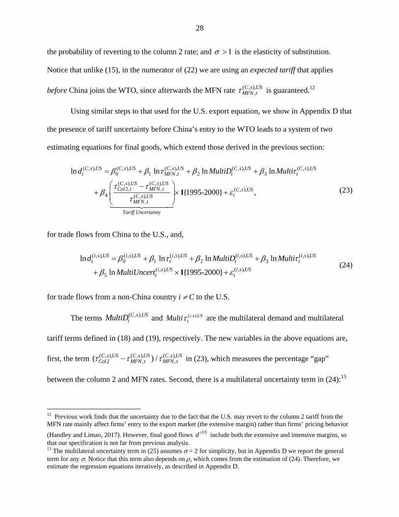
the probability of reverting to the column 2 rate; and 1 is the elasticity of substitution.

Notice that unlike (15), in the numerator of (22) we are using an expected tariff that applies

before China joins the WTO, since afterwards the MFN rate ( , ),,

C s USMFN t is guaranteed.12

Using similar steps to that used for the U.S. export equation, we show in Appendix D that

the presence of tariff uncertainty before China’s entry to the WTO leads to a system of two

estimating equations for final goods, which extend those derived in the previous section:

( , ), ( , ), ( , ), ( , ), ( , ),0 1 , 2 3

( , ), ( , ),2, , ( , ),

4 ( , ),,

ln ln ln ln

{1995-2000} ,

C s US C s US C s US C s US C s USt MFN t t t

C s US C s USCol t MFN t C s US

tC s USMFN t

Tariff Uncertainty

d MultiD Multi

1

(23)

for trade flows from China to the U.S., and,

( , ), ( , ), ( , ), ( , ), ( , ),0 1 2 3

( , ), ( , ),5

ln ln ln ln

ln {1995-2000}

i s US i s US i s US i s US i s USt t t t

i s US i s USt t

d MultiD Multi

MultiUncert

1 (24)

for trade flows from a non-China country i C to the U.S.

The terms ( , ),C s UStMultiD and USsi

tMulti ),,( are the multilateral demand and multilateral

tariff terms defined in (18) and (19), respectively. The new variables in the above equations are,

first, the term ( , ), ( , ), ( , ),, ,2( ) /C s US C s US C s US

MFN t MFN tCol in (23), which measures the percentage “gap”

between the column 2 and MFN rates. Second, there is a multilateral uncertainty term in (24):13

12 Previous work finds that the uncertainty due to the fact that the U.S. may revert to the column 2 tariff from the MFN rate mainly affect firms’ entry to the export market (the extensive margin) rather than firms’ pricing behavior

(Handley and Limao, 2017). However, final good flows ,i USd include both the extensive and intensive margins, so that our specification is not far from previous analysis. 13 The multilateral uncertainty term in (25) assumes = 2 for simplicity, but in Appendix D we report the general term for any . Notice that this term also depends on , which comes from the estimation of (24). Therefore, we estimate the regression equations iteratively, as described in Appendix D.

29

( , ),( , ), ( , ), ( , ),

2 ,, ,1

C s USi s US C s US C s US

t Col MFN ti US i US

k i

dMultiUncert

d

, (25)

which measures the added exports from non-Chinese countries who do not face this tariff

uncertainty. Because the uncertainty was present until 2001, when China joined the WTO, these

uncertainty variables are interacted with the dummy variable {1995-2000}1 which equals unity

between 1995 and 2000. The regression coefficients satisfy 1 ( 1) , 2 3 5 1 ,

and 4 ( 1) from which it follows that is estimated as the ratio 1 4/ .

The hypothetical final good flows from China to the U.S. when tariff levels remain at

the 1995 are found by plugging jsCMFN

),,(1995, into the regression result from (23):

( , ), ( , ), ( , ), ( , ), ( , ),0 1 ,1995 2 3

1995

( , ), ( , ),2, , ( , ),

4 ( , ),,

ˆ ˆ ˆ ˆ ˆln ln ln ln

ˆ ˆ{1995-2000} .

C s US C s US C s US C s US C s USt MFN t t

C s US C s USCol t MFN t C s US

tC s USMFN t

d MultiD Multi

1 (26)

The hypothetical imports from China when each of the other factors were fixed at the 1995 level,

1995

( , ),ln C s USt MultiD MultiD

d

, 1995

( , ),ln C s USt Multi Multi

d

, and 1995

( , ),ln C s USt Uncert Uncert

d

are found by

replacing each of the variables with the one from 1995, and likewise for the U.S. imports from

China of intermediate goods.

With these regression results, we then calculate the employment effect of U.S. imports

from China. For example, the employment effect of imports from China when tariff levels are

fixed at their 1995 level is:

,1, 1 11995, 1995,

ˆ ˆ( ) ( ) IMIMt t t t t t t

L Λ I A D Λ I A D

where,

30

19951995

1995

1,

2,

, ,,

( ) 1, ,

,

ˆ( )ˆ

ˆ( )

ktk

ktk

C US C kt tIM k US

t

N SUS US US kt tk US

N ktk

d

d

d dD

d d

d

is the hypothetical final demand vector when tariff levels imposed by the U.S. were fixed at their

1995 level. Elements of 1995,ˆ( )C USt

d are obtained from (26), and the corresponding estimates of

1995,ˆ( )US USt

d are obtained by using 1995,ˆ( )C USt

d in (10) and (11). The effect through multilateral

final demand 1,1995,

ˆ IM MultiDtL , the multilateral tariff 1,

1995,ˆ IM Multi

tL , and the uncertainty measure

1,1995,

ˆ IM UncerttL are estimated by taking similar steps.

The employment effect of imports of final and intermediate goods from China through a

change in tariffs imposed by the U.S. is estimated as:

, ,2, 1 11995, 1995, 1995,

ˆˆ ˆ( ) ( )IM IMIMt t t t t t t


where the elements of ,1995,

ˆ IMtA for China’s sales to the U.S. use the prediction like in (26), but for

intermediates, to obtain:

1995

( , ),( , ) , ( , ),( , ) ,1995,ˆ ˆ( ) /C r US s IM C s US r US s

t t ta x y

.

Then the input-output coefficients for the U.S. are computed using the predicted value of

Chinese sales 1995

( , ),( , )ˆ C s US rtx

within the market share regressions (13) and (14). The same

computation procedure applies to the effect though the multilateral final demand 2,1995,

ˆ IM MultiDtL , the

31

multilateral tariff 2,1995,

ˆ IM Multit

L , and the uncertainty measure 2,1995,

ˆ IM UncerttL .

5.3 Trade Flow Regression Results

The trade flow regressions are estimated over industries in the merchandise sector.14 The

first two columns in Table 8 report the estimates of (17) for U.S. exports, while the last two

columns estimate (23) and (24) for U.S. imports. Odd number columns use the log of bilateral

final good flows as the dependent variable, while even number columns use the log of bilateral

intermediate flows. All coefficients have the expected signs: the log of tariffs have negative signs,

meaning that tariff cuts have been contributing to increase the U.S. exports as well as U.S.

imports. The multilateral final demand term has positive signs, indicating that final demand of

trading partners increases U.S. exports and final demand of the U.S. also works to increase U.S.

imports. The multilateral tariff term has the expected positive sign, so a reduction of tariffs

imposed by other countries on their trading partners will reduce U.S. exports.

In addition to these three variables, the uncertainty measure and the multilateral

uncertainty term are introduced in predicting U.S. imports. The uncertainty measure interacted

with the dummy variable (taking the value one during 1995-2000) is negative and highly

significant, meaning that U.S. imported less from China less due to policy uncertainty before its

WTO entry. The multilateral uncertainty term has a positive sign, implying that other countries

besides China were able to export to the U.S. more due to the policy uncertainty on Chinese

tariffs in the U.S. After China’s accession to WTO in 2001, the policy uncertainty is eliminated.

14 One of the reasons we do not attempt to model service exports or imports, is that these can reflect the headquarters activities of multinational firms located in a third country, which are explicitly considered in Markusen (1984) and Ekholm, Forslid and Markusen (2007). For example, U.S. firms make earnings by selling a product designed in the U.S. to the rest of the world, which are recorded in the balance of payments as U.S. exports. However, it can be the case that some of the earnings are actually going to a multinational firm located in a third-country, say Ireland. This implies that there is a possibility that a part of our estimates of the service sector job gains include job gains that should be attributed to multinational firms located in a third country.

32

As a result, China’s exports to the U.S. increased and exports from other countries to the U.S.

decreased. As discussed in the previous section, the probability to reverting to the column 2 rate

is estimated as the ratio 1 4ˆ ˆ/ = -0.42/-2.79 = 0.15 for final goods and 1 4

ˆ ˆ/ = -0.64/-2.87 =

0.22 for intermediate good flows. These estimates are close to the probability of the column 2

tariff as estimated by Handley and Limao (2017).

The predicted values from these regressions are used in order to find hypothetical trade

flows in situations that each of these variables are kept at the 1995 level. The regression results

from columns (1) and (2) are used to decompose the employment effect of export expansion,

while the results from columns (3) and (4) are used to decompose the employment effect of

imports from China.

5.4 Results from the Decomposition Exercises

Table 9 reports the decomposition results for the employment effect of export expansion.

Panel A takes in account only final good exports, while the panel B considers both final good

and intermediate exports. Panel A, columns (2) and (3) shows that in the manufacturing industry,

8.7% and 60.3% of the added labor demand from export expansion are due to tariff cuts by

trading partners of the U.S. and their final demand, respectively. The multilateral tariff in column

(4) explains a small negative portion (-2.5%), so in total, two-thirds of the added labor demand is

explained by these exogenous factors. The remaining one-third is unexplained, as shown in

column (5), and is due to the residual in the estimated export equation.

Scanning down column (5) of panel A, we see that somewhat more than one-third of the

employment effect of exports is left unexplained in the natural resource and service sectors, but

in panel B when intermediates are included, this unexplained portion is less than 40%. There are

many other factors that could account for U.S. exports that we have not taken account of: for

33

example, Feenstra, Ma and Xu (2017) include the bilateral exports of the same eight industrial

countries used by Autor, Dorn, and Hanson (2013, 2015), but now to explain U.S. exports, and

they find that this additional instrument makes a difference. Evidently, our “multilateral demand”

variable that we have included in the export equation is not capturing the same information.

More generally, the R2 values on our trade flow regressions in Table 8 are not high enough to

expect these variables to fully account for export flows.

Table 10 report the decomposition results for the fall in labor demand due to U.S. imports

from China based on the IV estimation result of the market share regression.15 The variable in

the import flow regression that accounts for the overwhelming portion of the is the fall in

demand in policy uncertainly associated with China’s WTO accession: eliminating the “gap”

between the column 2 and the MFN tariffs in column (5) accounts for 47-50% of the

manufacturing job losses. These estimates are consistent with previous literature investigating

the impact of elimination of policy uncertainty due to China’s accession to WTO in 2001. For

example, Pierce and Schott (2016) demonstrate that a change in U.S. policy uncertainty related

with the U.S.-China Normal Trade Relation gap has a statistically significant impact on the

decline of manufacturing employment in the U.S. Also, many other work find the sizable impact

of China’s accession to WTO on the growth of China’s exports (Feng, Li, and Swenson, 2017;

Crowley, Song, and Meng, 2016; Handley and Limao, 2017).16 Handley and Limao (2017) show

that the reduction of policy uncertainty can explain 22-30% of China’s export growth to the U.S.

between 2001 and 2005.

15 See Appendix E for the decomposition result based on the OLS estimates. The results are very similar to those based on the IV estimates. 16 Feng, Li, and Swenson (2017) show that at the product level, the reduction in tariff uncertainty due to China’s accession to WTO increased the entry of Chinese firms for export to the U.S. market. Crowley, Song, and Meng (2016) find that 36% of new entrants per year after 2011 are explained by China’s entry into the WTO.

34

Our estimates of the 47-50% contribution of the policy uncertainty reduction on the

decline of manufacturing employment are somewhat greater than Handley and Limao’s finding.

There are at least three reasons for our higher estimates. First, we explain the job losses during

1995-2011 while Handley and Limao (2017) use the data from 2001-2005. As was shown in

Figure 1, there is a sizable increase in Chinese exports to the U.S. after 2005. Therefore, this

difference in the data period is partially responsible for the difference between our estimates and

theirs. Second, Handley and Limao’s estimates are based on a general equilibrium model, which

includes a feedback from the labor market equilibrium. In contrast, we do not attempt to close

the model and only focus on a change in the demand-side of the labor market. Third, we use the

35 sectoral data from the WIOD database while Handley and Limao (2017) use the HS-6 digit

level data from the NBER Harmonized System Imports by Commodity and Country. In other

words, our estimates are based on a more aggregated macro dataset while Handley and Limao

(2017) employ a micro dataset.

The direct reduction in MFN tariffs on China (column 2) accounts for only a small effect,

as does the change in multilateral tariffs (column 4). The multilateral final demand variable

(column 3) explains a significant portion of the job losses only in the natural resource sector.

Overall, from column (6) we see that the unexplained portion of the job losses are somewhat

higher than one-third, but less than 40% when intermediate goods are included in the analysis.

Like we have argued for U.S. exports, there are many other factors that can explain the rise in

merchandise imports from China that we have not included in our trade flow regressions, which

would appear in the unexplained residual.17

17 As mentioned in note 2, Amiti, Dai, Feenstra and Romalis (2017) find that the growth in U.S, imports from China (and the accompany consumer benefits in the United States) are due more to China’s reduction in its own tariffs on intermediate inputs than the reduction in the uncertainty of tariffs in the U.S.

35

6. Conclusions

This paper has examined the employment effect of U.S. exports, imports, and imports

from China on the U.S. labor market by applying an input-output analysis. We find that the

growth in U.S. merchandise exports over 1995-2011 led to demand for 1.9 million jobs in

manufacturing, 0.45 million in resource industries, and 1.3 million jobs in services, totaling 3.7

million. In comparison, U.S. merchandise imports from China over 1995-2011 led to reduced

labor demand of 1.4 million jobs in manufacturing and 0.6 million in services (with small losses

in resource industries), for total job losses of 2.0 million. It follows that the expansion in U.S.

merchandise exports relative to imports from China over 1995-2011 led to the net demand for

about 1.7 million jobs. Comparing the growth of U.S. merchandise exports to merchandise

imports from all countries, we find a fall in net labor demand due to trade, but comparing the

growth of total U.S. exports to total imports from all countries, then there is a rise in net labor

demand because of the growth in service exports.

It is surprising that our estimates of the job impacts of trade are not that different from

existing literature, which uses industry (or commuting zone) regressions to infer the equilibrium

impact on employment. The added demand for 1.9 million jobs in U.S. manufacturing exports

that we have found much the same as the equilibrium increase of 1.9 million jobs for a 12 year

period, 1999-2011, estimated by Feenstra, Ma and Xu (2017). That added demand for

manufacturing jobs explains about one-half of the overall demand increase of 3.7 million jobs

due to merchandise exports. The offsetting reduction in labor demand of 2.0 million jobs due to

imports from China, mainly manufactures, is very close to Acemoglu, Autor, Dorn, Hanson and

Price (2016), who find about 1.0 million manufacturing jobs lost in equilibrium during 1999-

2011, and another 1.0 million jobs lost by intermediate demand throughout the economy.

36

Because the input-output analysis relies exclusively on the demand side of the labor

market, one might have expected to get considerably larger shifts in demand that would then be

offset by upward-sloping labor supply curves to obtain the (smaller) equilibrium changes.

Instead, our findings are that the demand shifts from the input-output analysis are similar to the

equilibrium changes in employment identified by regression analysis. There are two possible

explanations for this result. The first is that there are near-horizontal labor supply curves at the

regional level, reflecting movement in and out of unemployment or labor force participation, or

movement between regions. But that is an unrealistic explanation: generally there is limited

mobility across regions, except for immigrants who do respond to wages difference across

regions (Caneda and Kovak, 2016) . A different explanation for this finding is that regions with

negative employment shocks from imports also have positive shocks from exports, so that the net

shocks in regions are smaller than the gross (export and imports) shocks. That explanation is

explored further in Feenstra, Ma and Xu (2017). Caliendo, Dvorkin and Parro (2015) and Dix-

Carneiro and Kovak (2017) also incorporate careful specifications of the employment decisions

and regional movement of individuals.

While we have not attempted to close our model with labor market equilibrium, we have

begun to address another criticism of input-output analysis, namely, that the changes in the trade

and production values as well as the input-output coefficients are all endogenous since they are

equilibrium values each year. That criticism is of the first-order when using regressions since the

coefficient estimates are then biased, and it is addressed with instrumental variables. We have

attempted here to address the same issue here, within input-output analysis, by breaking up the

total change in the endogenous trade values into exogenous portions due to various causes. In

particular, we have tried to exploit the changes in bilateral tariffs – including the reduction in the

37

uncertainly on U.S. tariffs facing China after it joined the WTO – to predict the changes in trade

flows. We have been only partially successful in this attempt. Using our structural equation for

U.S. exports and imports to identify the exogenous portion of these changes, we explain nearly

two-thirds of the measured employment impacts for both U.S. exports and for imports from

China. It should be recognized that explaining even that amount in an input-output framework is

an achievement: Caliendo, Dvorkin and Parro (2015) also use WIOD, for example, and they rely

on an assumed productivity shock in China rather than the tariff changes to explain the surge in

exports. It can be hoped that the identification of exogenous factors leading to changes in trade

and the associated labor demand, and their incorporation into a general equilibrium framework,

can be improved in future work.

References

Acemoglu, Daron, David Autor, David Dorn, Gordon H. Hanson and Brendan Price, 2016, “Import Competition and the Great U.S. Employment Sag of the 2000s,” Journal of Labor Economics, 34(S1), S141 - S198.

Amiti, Mary, Mi Dai, Robert Feenstra and John Romalis, 2017, “How Did China’s WTO Entry Benefit U.S. Consumers?” NBER Working Paper no. 23487.

Autor, David H., David Dorn, and Gordon H. Hanson, 2013, "The China Syndrome: Local Labor Market Effects of Import Competition in the United States," American Economic Review, 103(6), 2013, 2121-68.

Autor, David H., David Dorn and Gordon H. Hanson, 2015, “Untangling Trade and Technology: Evidence from Local Labor Markets,” Economic Journal, 125(584), May, 621–646.

Autor, David H., David Dorn, Gordon H. Hanson and Jae Song, 2014. "Trade Adjustment: Worker-Level Evidence," Quarterly Journal of Economics, 129(4), 1799-1860.

Caliendo, Lorenzo, Maximiliano Dvorkin and Fernando Parro, 2015, “The Impact of Trade on Labor Market Dynamics,” NBER Working Paper no. 21149.

Caliendo, Lorenzo, Robert Feenstra, John Romalis and Alan M. Taylor, 2016, “Tariff Reductions, Entry, and Welfare: Theory and Evidence for the Last Two Decades,” NBER Working Paper No. 21768.

38

Cadena, Brian C. and Brian Kovak, 2016, “Immigrants Equilibrate Local Labor Markets: Evidence from the Great Recession,” American Economic Journal: Applied Economics, 8(1), 257-290

Crowley, Meredith A., Huasheng Song, and Ning Meng (2016) “Tariff Scares: Trade Policy Uncertainty and Foreign Market Entry by Chinese Firms”, University of Cambridge and Zhejian University.

Dix-Carneiro, Rafael and Brian Kovak, 2017, “Trade Liberalization and Regional Dynamics” American Economic Review, forthcoming.

Ekholm, Karolina, Rikard Forslid, and James R. Markusen (2007) “Export-Platform Foreign Direct Investment,” Journal of European Economic Association, 5 (4), 776-795.

Feenstra, Robert C., Robert Inklaar, and Marcel P. Timmer, 2015, “The Next Generation of the Penn World Table,” American Economic Review, 105 (10), pp. 3150-3182.

Feenstra, Robert C. and Akira Sasahara, 2017, “The ‘China Shock’ in Trade: Consequences for ASEAN and East Asia,” University of California, Davis, and University of Idaho.

Feenstra, Robert C., Hong Ma and Yuan Xu, 2017, “U.S. Exports and Employment,” University of California, Davis and Tsinghua University, Beijing.

Feng, Ling, Zhiyuan Li and Deborah L. Swenson, 2017, “Trade Policy Uncertainty and Exports: Evidence from China's WTO Accession,” Journal of International Economics, 106, 20-36.

Handley, Kyle and Nuno Limão, 2017, “Policy Uncertainty, Trade and Welfare: Theory and Evidence for China and the U.S.,” American Economic Review, forthcoming.

International Monetary Fund, 2017, World Economic Outlook Update: A Shifting Global Economic Landscape, January 2017, Washington D.C.

Johnson, Robert and Guillermo Noguera, 2012, “Accounting for Intermediates: Production Sharing and Trade in Value Added,” Journal of International Economics, 86 (2), 224-236.

Leontief, Wassily W., 1936, “Quantitative Input-Output Relations in the Economic System of the United States,” Review of Economics and Statistics, 18 (3), pp. 105-125.

Los, Bart, Marcel P. Timmer and Gaaitzen J. de Vries, 2015, “How Important are Exports for Job Growth in China? A Demand-side Analysis,” Journal of Comparative Economics, 43(1), 19-32.

Los, Bart, Marcel P. Timmer, Gaaitzen J. de Vries, 2016, “Tracing Value-Added and Double Counting in Gross Exports: Comment,” American Economic Review, 106 (7), 1958-1966.

Markusen, James R. (1984) “Multinationals, Multi-Plant Economies, and the Gains from Trade,” Journal of International Economics, 16 (3-4), 205-226.

39

Pierce, Justin R. and Peter K. Schott, 2016, “The Surprisingly Swift Decline of U.S. Manufacturing Employment,“ American Economic Review, 106(7), 1632-62.

Romalis, John, 2007, “NAFTA's and CUSFTA's Impact on International Trade,” Review of Economics and Statistics, 89(3), August, 416-35.

Timmer, Marcel P., Abdul Azeez Erumban, Bart Los, Robert Stehrer, and Gaaitzen J. de Vries, 2014, “Slicing Up Global Value Chains,” Journal of Economic Perspectives, 28 (2), 99-118.

Timmer, Marcel P., Dietzenbacher, E., Los, B., Stehrer, R. and de Vries, G. J., 2015, “An Illustrated User Guide to the World Input–Output Database: the Case of Global Automotive Production,” Review of International Economics 23, 575–605.

Vianna, Andre C., 2016, “The Impact of Exports to China on Latin American Growth,” Journal of Asian Economics, 47 (1), 58-66.

Wang , Zhi, Shang-Jin Wei, Xinding Yu, and Kunfu Zhu, 2017, “Re-examining the Impact of the China Trade Shock on the US Labor Market: A Value-Chain Perspective,” University of International Business and Economics, Beijing, and Columbia University.

Wood, Adrian, 2017, “The 1990s Trade and Wages Debate in Retrospect,” University of Oxford.

World Bank, 2017, “Where We Work: China Overview”, World Bank, Washington D.C., available at http://www.worldbank.org/en/country/china/overview.

40

Figure 1: Import and Export Shares in the U.S.

Notes: The figure shows the U.S. aggregate export value, the U.S. aggregate import value, and the U.S. import value from China as a share of U.S. GDP. The data on exports and imports are from the WIOD Input-Output Table where both final goods and intermediate goods are included.

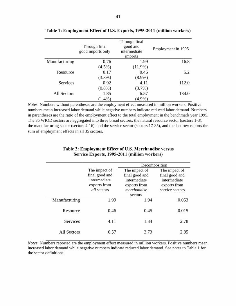
41

Table 1: Employment Effect of U.S. Exports, 1995-2011 (million workers)

Through final good imports only

Through final good and

intermediate imports

Employment in 1995

Manufacturing 0.76 1.99 16.8 (4.5%) (11.9%)

Resource 0.17 0.46 5.2 (3.3%) (8.9%)

Services 0.92 4.11 112.0 (0.8%) (3.7%)

All Sectors 1.85 6.57 134.0 (1.4%) (4.9%)

Notes: Numbers without parentheses are the employment effect measured in million workers. Positive numbers mean increased labor demand while negative numbers indicate reduced labor demand. Numbers in parentheses are the ratio of the employment effect to the total employment in the benchmark year 1995. The 35 WIOD sectors are aggregated into three broad sectors: the natural resource sector (sectors 1-3), the manufacturing sector (sectors 4-16), and the service sector (sectors 17-35), and the last row reports the sum of employment effects in all 35 sectors.

Table 2: Employment Effect of U.S. Merchandise versus Service Exports, 1995-2011 (million workers)

The impact of final good and intermediate exports from

all sectors

Decomposition The impact of final good and intermediate exports from merchandise

sectors

The impact of final good and intermediate exports from

service sectors

Manufacturing 1.99 1.94 0.053

Resource 0.46 0.45 0.015

Services 4.11 1.34 2.78

All Sectors 6.57 3.73 2.85

Notes: Numbers reported are the employment effect measured in million workers. Positive numbers mean increased labor demand while negative numbers indicate reduced labor demand. See notes to Table 1 for the sector definitions.

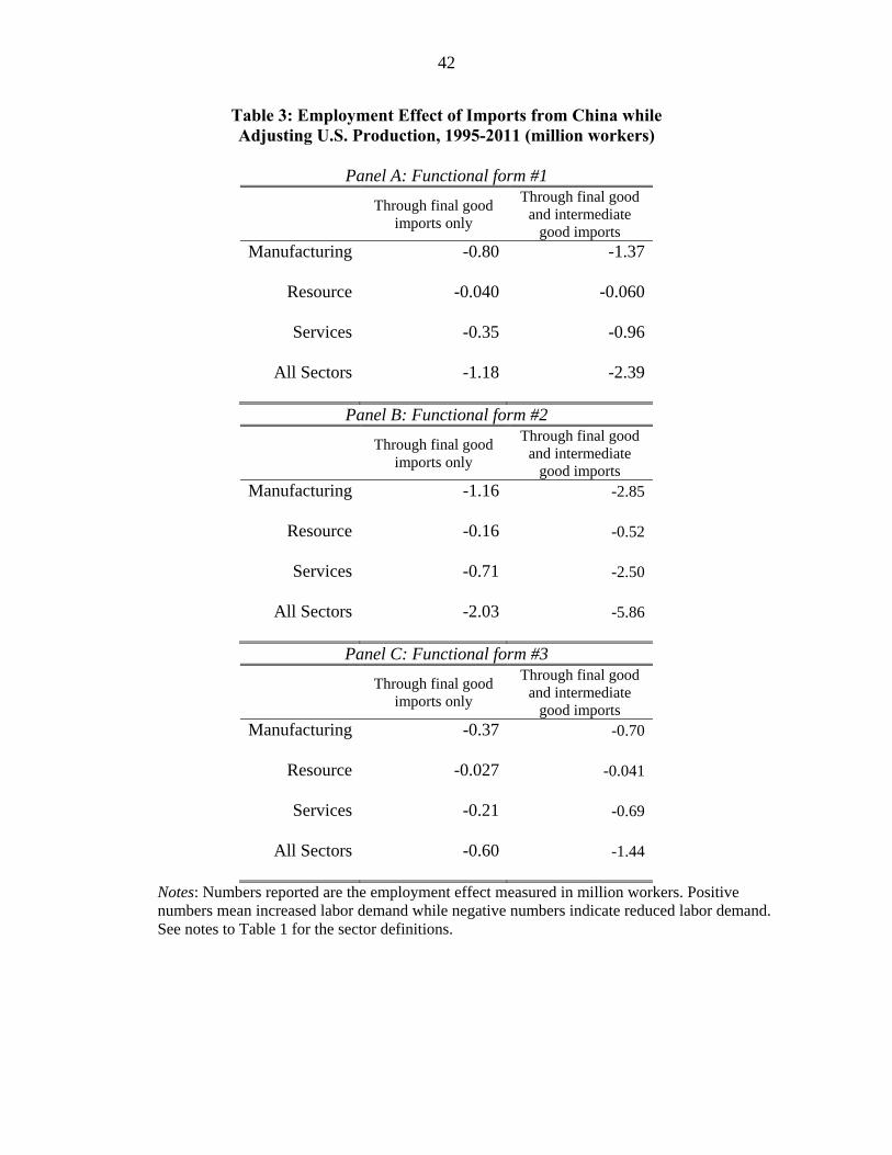
42

Table 3: Employment Effect of Imports from China while Adjusting U.S. Production, 1995-2011 (million workers)

Panel A: Functional form #1


Through final good and intermediate

good imports Manufacturing -0.80 -1.37

Resource -0.040 -0.060

Services -0.35 -0.96

All Sectors -1.18 -2.39

Panel B: Functional form #2




Resource -0.16 -0.52



Panel C: Functional form #3




Resource -0.027 -0.041




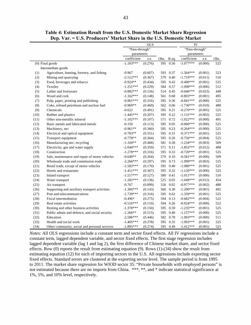
43

Table 4: Estimation Result from the U.S. Domestic Market Share Regression Dep. Var. = U.S. Producers’ Market Share in the U.S. Domestic Market

Notes: All OLS regressions include a constant term and sector fixed effects. All IV regressions include a constant term, lagged dependent variable, and sector fixed effects. The first stage regression includes lagged dependent variable (lag 1 and lag 2), the first difference of Chinese market share, and sector fixed effects. Row (0) reports the result from estimating equation (9). Rows (1)-(34) show the result from estimating equation (12) for each of importing sectors in the U.S. All regressions include exporting sector fixed effects. Standard errors are clustered at the exporting sector level. The sample period is from 1995 to 2011. The market share regression for WIOD sector 35: “Private households with employed persons” is not estimated because there are no imports from China. ***, **, and * indicate statistical significance at 1%, 5%, and 10% level, respectively.

coefficient s.e. coefficient s.e.(0) -1.103*** (0.276) 595 0.56 -1.077*** (0.000) 525

(1) Agriculture, hunting, forestry, and fishing -0.967 (0.607) 593 0.37 -1.564*** (0.001) 523(2) Mining and quarrying -2.512*** (0.367) 579 0.40 -1.719*** (0.011) 510(3) Food, beverages and tobacco -0.924** (0.434) 595 0.42 -0.490*** (0.001) 525(4) Textiles -1.251*** (0.229) 584 0.57 -1.098*** (0.006) 512(5) Lather and footweare -0.882*** (0.156) 514 0.45 -0.646*** (0.023) 448(6) Wood and cork -1.162*** (0.148) 561 0.68 -0.803*** (0.001) 495(7) Pulp, paper, printing and publishing -0.961*** (0.316) 595 0.36 -0.841*** (0.000) 525(8) Coke, refined petroleum and nuclear fuel -0.969** (0.469) 562 0.06 -1.730*** (0.010) 488(9) Chemicals -0.622 (0.491) 595 0.21 -0.270*** (0.005) 525

(10) Rubber and plastics -1.445*** (0.207) 595 0.22 -1.131*** (0.002) 525(11) Other non-metallic mineral -1.102*** (0.107) 571 0.72 -1.022*** (0.000) 495(12) Basic metals and fabricated metals -0.150 (0.113) 595 0.05 -0.060*** (0.000) 525(13) Machinery, nec -0.961** (0.360) 595 0.23 -0.264*** (0.000) 525(14) Electrical and optical equipment -0.783** (0.351) 595 0.31 -0.371*** (0.001) 525(15) Transport equipment -0.778** (0.364) 595 0.26 -0.756*** (0.004) 525(16) Manufacturing nec; recycling -1.104** (0.468) 581 0.28 -1.234*** (0.003) 509(17) Electricity, gas and water supply -2.044*** (0.359) 571 0.11 -1.852*** (0.012) 498(18) Construction -1.278*** (0.316) 595 0.33 -0.720*** (0.001) 525(19) Sale, maintenance and repair of motor vehicles -0.649** (0.264) 579 0.10 -0.581*** (0.000) 509(20) Wholesale trade and commission trade -2.266*** (0.297) 595 0.73 -1.999*** (0.003) 525(21) Retail trade, except of motor vehicles -1.583*** (0.170) 595 0.40 -1.080*** (0.001) 525(22) Hotels and restaurants -1.411*** (0.367) 595 0.32 -1.120*** (0.000) 525(23) Inland transport -1.517*** (0.127) 580 0.41 -1.011*** (0.000) 510(24) Water transport -1.282*** (0.136) 525 0.05 -1.049*** (0.012) 454(25) Air transport -0.767 (0.899) 556 0.02 -0.977*** (0.002) 488(26) Supporting and auxiliary transport activities -1.306*** (0.143) 560 0.30 -1.200*** (0.001) 492(27) Post and telecommunications -1.739*** (0.316) 595 0.62 -1.359*** (0.001) 525(28) Fiscal intermediation -0.496* (0.275) 594 0.13 -0.682*** (0.004) 522(29) Real estate activities -0.516*** (0.110) 594 0.26 -0.924*** (0.000) 522(30) Renting and other business activities -1.378*** (0.150) 595 0.59 -1.235*** (0.001) 525(31) Public admin and defence, and social security -1.266** (0.515) 595 0.40 -1.157*** (0.000) 525(32) Education -2.586*** (0.446) 582 0.78 -1.993*** (0.000) 511(33) Health and social work -1.405*** (0.378) 595 0.35 -1.093*** (0.001) 525(34) Other community, social and personal services -1.895*** (0.274) 595 0.49 -1.412*** (0.001) 525

OLS IV“Pass-through”

parameters

Obs.Obs.Final goodsIntermediate goods

R-sq.

“Pass-through” parameters

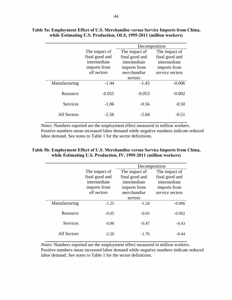
44

Table 5a: Employment Effect of U.S. Merchandise versus Service Imports from China, while Estimating U.S. Production, OLS, 1995-2011 (million workers)

The impact of final good and intermediate imports from

all sectors

Decomposition The impact of final good and intermediate imports from merchandise

sectors


service sectors

Manufacturing -1.44 -1.43 -0.006

Resource -0.055 -0.053 -0.002

Services -1.06 -0.56 -0.50

All Sectors -2.56 -2.04 -0.51


Table 5b: Employment Effect of U.S. Merchandise versus Service Imports from China, while Estimating U.S. Production, IV, 1995-2011 (million workers)


all sectors

Decomposition The impact of final good and intermediate imports from merchandise

sectors


service sectors

Manufacturing -1.25 -1.24 -0.006

Resource -0.05 -0.05 -0.002

Services -0.90 -0.47 -0.43

All Sectors -2.20 -1.76 -0.44


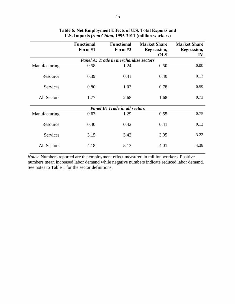
45

Table 6: Net Employment Effects of U.S. Total Exports and U.S. Imports from China, 1995-2011 (million workers)

Functional Form #1

Functional Form #3

Market Share Regression,

OLS

Market Share Regression,

IVPanel A: Trade in merchandise sectors

Manufacturing

0.58 1.24 0.50 0.00

Resource

0.39 0.41 0.40 0.13

Services

0.80 1.03 0.78 0.59

All Sectors

1.77 2.68 1.68 0.73

Panel B: Trade in all sectors Manufacturing

0.63 1.29 0.55 0.75

Resource

0.40 0.42 0.41 0.12

Services

3.15 3.42 3.05 3.22

All Sectors

4.18 5.13 4.01 4.38


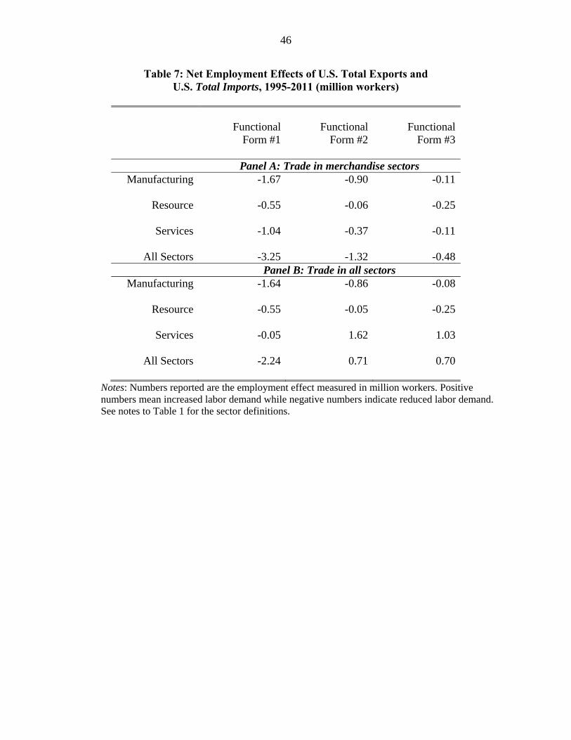
46

Table 7: Net Employment Effects of U.S. Total Exports and U.S. Total Imports, 1995-2011 (million workers)

Functional Form #1

Functional

Form #2Functional

Form #3

Panel A: Trade in merchandise sectors Manufacturing -1.67 -0.90 -0.11

Resource -0.55 -0.06 -0.25

Services -1.04 -0.37 -0.11

All Sectors -3.25 -1.32 -0.48

Panel B: Trade in all sectors Manufacturing -1.64 -0.86 -0.08

Resource -0.55 -0.05 -0.25

Services -0.05 1.62 1.03

All Sectors -2.24 0.71 0.70


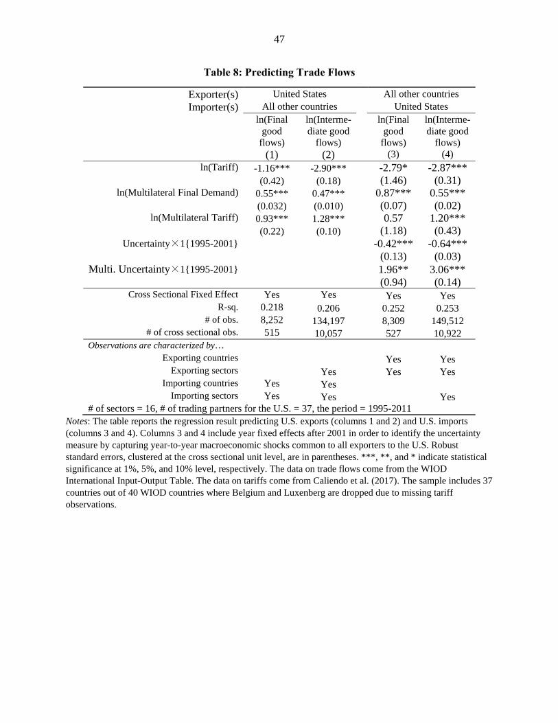
47

Table 8: Predicting Trade Flows

Exporter(s) United States All other countries Importer(s) All other countries United States

ln(Final good

flows)

ln(Interme-diate good

flows)

ln(Final good

flows)

ln(Interme-diate good

flows) (1) (2) (3) (4)

ln(Tariff) -1.16*** -2.90*** -2.79* -2.87*** (0.42) (0.18) (1.46) (0.31)

ln(Multilateral Final Demand) 0.55*** 0.47*** 0.87*** 0.55*** (0.032) (0.010) (0.07) (0.02)

ln(Multilateral Tariff) 0.93*** 1.28*** 0.57 1.20*** (0.22) (0.10) (1.18) (0.43)

Uncertainty×1{1995-2001} -0.42*** -0.64*** (0.13) (0.03)

Multi. Uncertainty×1{1995-2001} 1.96** 3.06*** (0.94) (0.14)

Cross Sectional Fixed Effect Yes Yes Yes Yes R-sq. 0.218 0.206 0.252 0.253

# of obs. 8,252 134,197 8,309 149,512 # of cross sectional obs. 515 10,057 527 10,922

Observations are characterized by… Exporting countries Yes Yes

Exporting sectors Yes Yes Yes Importing countries Yes Yes

Importing sectors Yes Yes Yes # of sectors = 16, # of trading partners for the U.S. = 37, the period = 1995-2011

Notes: The table reports the regression result predicting U.S. exports (columns 1 and 2) and U.S. imports (columns 3 and 4). Columns 3 and 4 include year fixed effects after 2001 in order to identify the uncertainty measure by capturing year-to-year macroeconomic shocks common to all exporters to the U.S. Robust standard errors, clustered at the cross sectional unit level, are in parentheses. ***, **, and * indicate statistical significance at 1%, 5%, and 10% level, respectively. The data on trade flows come from the WIOD International Input-Output Table. The data on tariffs come from Caliendo et al. (2017). The sample includes 37 countries out of 40 WIOD countries where Belgium and Luxenberg are dropped due to missing tariff observations.

48

Table 9: Explaining the Employment Effect of Merchandise Exports, 1995-2011 (million workers)

Decomposition

Tariff Cuts Multilateral

Final Demand Multilateral

Tariff Residuals

The overall

effect of exports

The effect through a

reduction of tariffs imposed

by trading partners on the

U.S.

The effect through an increase in multilateral

demand term

The effect through a decrease of the multilateral tariff

term

The unexplained

part

(1) (2) (3) (4) (5) Panel A: Through final good exports only

Manufacturing 0.753 0.065 0.454 -0.019 0.253 [8.7%] [60.3%] [-2.5%] [33.6%]

Resource 0.169 0.016 0.080 -0.005 0.079 [9.3%] [47.1%] [-2.9%] [46.6%]

Services 0.517 0.040 0.287 -0.012 0.203 [7.7%] [55.5%] [-2.4%] [39.2%]

All Sectors 1.440 0.121 0.821 -0.036 0.535 [8.4%] [57.0%] [-2.5%] [37.1%] Panel B: Through final good and intermediate exports

Manufacturing 1.937 0.293 1.063 -0.062 0.643 [15.2%] [54.9%] [-3.2%] [33.2%]

Resource 0.449 0.092 0.187 -0.006 0.177 [20.4%] [41.7%] [-1.4%] [39.4%]

Services 1.339 0.185 0.670 -0.032 0.516 [13.8%] [50.0%] [-2.4%] [38.5%]

All Sectors 3.725 0.570 1.920 -0.101 1.336 [15.3%] [51.5%] [-2.7%] [35.9%]

Notes: Numbers without brackets are the employment effect measured in million workers. Positive numbers mean increased labor demand while negative numbers indicate reduced labor demand. Numbers in square brackets are the ratio of each component of the employment effect to the overall employment effect. See notes to Table 1 for the sector definitions.

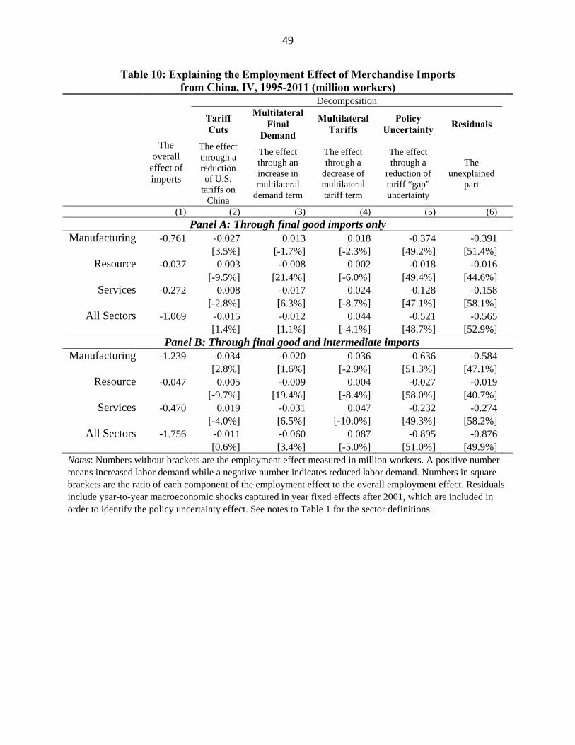
49

Table 10: Explaining the Employment Effect of Merchandise Imports from China, IV, 1995-2011 (million workers)

The overall

effect of imports

Decomposition

Tariff Cuts

Multilateral Final

Demand

Multilateral Tariffs

Policy Uncertainty

Residuals

The effect through a reduction of U.S.

tariffs on China


demand term


decrease of multilateral tariff term


reduction of tariff “gap” uncertainty

The unexplained

part

(1) (2) (3) (4) (5) (6)

Panel A: Through final good imports only Manufacturing -0.761 -0.027 0.013 0.018 -0.374 -0.391

[3.5%] [-1.7%] [-2.3%] [49.2%] [51.4%]Resource -0.037 0.003 -0.008 0.002 -0.018 -0.016

[-9.5%] [21.4%] [-6.0%] [49.4%] [44.6%]Services -0.272 0.008 -0.017 0.024 -0.128 -0.158

[-2.8%] [6.3%] [-8.7%] [47.1%] [58.1%]All Sectors -1.069 -0.015 -0.012 0.044 -0.521 -0.565

[1.4%] [1.1%] [-4.1%] [48.7%] [52.9%] Panel B: Through final good and intermediate imports

Manufacturing -1.239 -0.034 -0.020 0.036 -0.636 -0.584 [2.8%] [1.6%] [-2.9%] [51.3%] [47.1%]

Resource -0.047 0.005 -0.009 0.004 -0.027 -0.019 [-9.7%] [19.4%] [-8.4%] [58.0%] [40.7%]

Services -0.470 0.019 -0.031 0.047 -0.232 -0.274 [-4.0%] [6.5%] [-10.0%] [49.3%] [58.2%]

All Sectors -1.756 -0.011 -0.060 0.087 -0.895 -0.876 [0.6%] [3.4%] [-5.0%] [51.0%] [49.9%]

Notes: Numbers without brackets are the employment effect measured in million workers. A positive number means increased labor demand while a negative number indicates reduced labor demand. Numbers in square brackets are the ratio of each component of the employment effect to the overall employment effect. Residuals include year-to-year macroeconomic shocks captured in year fixed effects after 2001, which are included in order to identify the policy uncertainty effect. See notes to Table 1 for the sector definitions.

50

Appendices

Appendix A: List of WIOD Sectors and Countries

Each country in the WIOD input-output table is comprised of 35 sectors. The list of the sectors is as follows. It also shows the definition of the agriculture, manufacturing and service sectors that we employ to aggregate the sectoral employment effect.

Table A1: List of 35 WIOD Sectors and the Definition of Aggregate Sectors

Notes: The table shows the list of 35 WIOD sectors and the definition of the three aggregate sectors in the main text.

No. WIOD Sector Aggregation1 Agriculture, hunting, forestry, and fishing2 Mining and quarrying3 Food, beverages and tobacco4 Textiles5 Lather and footweare6 Wood and cork7 Pulp, paper, printing and publishing8 Coke, refined petroleum and nuclear fuel9 Chemicals

10 Rubber and plastics11 Other non-metallic mineral12 Basic metals and fabricated metals13 Machinery, nec14 Electrical and optical equipment15 Transport equipment16 Manufacturing nec; recycling17 Electricity, gas and water supply18 Construction19 Sale, maintenance and repair of motor vehicles and motorcycles20 Wholesale trade and commission trade, except of motor vehicles21 Retail trade, except of motor vehicles and motorcycles22 Hotels and restaurants23 Inland transport24 Water transport25 Air transport26 Supporting and auxiliary transport activities; activities of travel agencies27 Post and telecommunications28 Fiscal intermediation29 Real estate activities30 Renting and other business activities31 Public admin and defence, and compulsory social security32 Education33 Health and social work34 Other community, social and personal services35 Private households with employed persons

Services (the tertiary sector)

Agriculture (the primary sector)

Manufacturing (the secondary

sector)

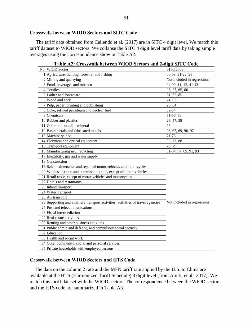
51

Crosswalk between WIOD Sectors and SITC Code

The tariff data obtained from Caliendo et al. (2017) are in SITC 4 digit level. We match this tariff dataset to WIOD sectors. We collapse the SITC 4 digit level tariff data by taking simple averages using the correspondence show in Table A2.

Table A2: Crosswalk between WIOD Sectors and 2-digit SITC Code

Crosswalk between WIOD Sectors and HTS Code

The data on the column 2 rate and the MFN tariff rate applied by the U.S. to China are available at the HTS (Harmonized Tariff Schedule) 8 digit level (from Amiti, et al., 2017). We match this tariff dataset with the WIOD sectors. The correspondence between the WIOD sectors and the HTS code are summarized in Table A3.

No. WIOD Sector SITC code1 Agriculture, hunting, forestry, and fishing 00-03, 21-22, 292 Mining and quarrying Not included in regressions3 Food, beverages and tobacco 04-09, 11, 12, 41-434 Textiles 26, 27, 65, 665 Lather and footweare 61, 62, 856 Wood and cork 24, 637 Pulp, paper, printing and publishing 25, 648 Coke, refined petroleum and nuclear fuel 32-349 Chemicals 51-56, 59

10 Rubber and plastics 23, 57, 5811 Other non-metallic mineral 6812 Basic metals and fabricated metals 28, 67, 69, 96, 9713 Machinery, nec 71-7614 Electrical and optical equipment 35, 77, 8815 Transport equipment 78, 7916 Manufacturing nec; recycling 81-84, 87, 89, 91, 9317 Electricity, gas and water supply18 Construction19 Sale, maintenance and repair of motor vehicles and motorcycles20 Wholesale trade and commission trade, except of motor vehicles21 Retail trade, except of motor vehicles and motorcycles22 Hotels and restaurants23 Inland transport24 Water transport25 Air transport26 Supporting and auxiliary transport activities; activities of travel agencies27 Post and telecommunications28 Fiscal intermediation29 Real estate activities30 Renting and other business activities31 Public admin and defence, and compulsory social security32 Education33 Health and social work34 Other community, social and personal services35 Private households with employed persons

Not included in regressions

52

Table A3: Crosswalk between WIOD Sectors and HTS Code

In the final demand matrix, each of the destination countries consist of five final demand categories, as follows:

1. Final consumption expenditure by households 2. Final consumption expenditure by non-profit organizations serving households (NPISH) 3. Final consumption expenditure by government 4. Gross fixed capital formation 5. Changes in inventories and valuables

In input-output calculation, we compute the sum of these.

No. WIOD Sector HTS code1 Agriculture, hunting, forestry, and fishing 01, 062 Mining and quarrying Not included in regressions3 Food, beverages and tobacco 02-05, 07-254 Textiles 50-675 Lather and footweare 41-436 Wood and cork 44, 457 Pulp, paper, printing and publishing 47-498 Coke, refined petroleum and nuclear fuel 27, 33, 34, 369 Chemicals 28-32, 38

10 Rubber and plastics 39, 40, 4611 Other non-metallic mineral 68-7012 Basic metals and fabricated metals 26, 72-76, 78-81

13 Machinery, nec 8414 Electrical and optical equipment 37, 85, 9015 Transport equipment 86, 87, 88, 8916 Manufacturing nec; recycling 35, 82, 83, 91-9717 Electricity, gas and water supply18 Construction19 Sale, maintenance and repair of motor vehicles and motorcycles20 Wholesale trade and commission trade, except of motor vehicles21 Retail trade, except of motor vehicles and motorcycles22 Hotels and restaurants23 Inland transport24 Water transport25 Air transport26 Supporting and auxiliary transport activities; activities of travel agencies27 Post and telecommunications28 Fiscal intermediation29 Real estate activities30 Renting and other business activities31 Public admin and defence, and compulsory social security32 Education33 Health and social work34 Other community, social and personal services35 Private households with employed persons

Not included in regressions

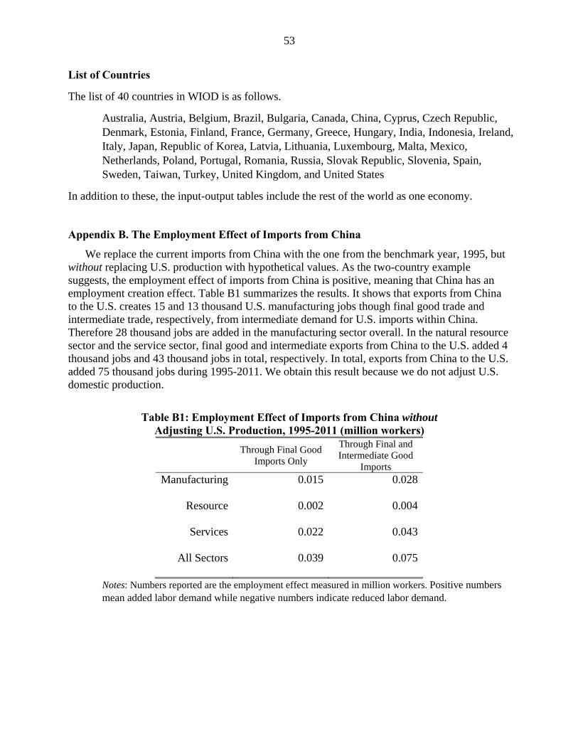
53

List of Countries

The list of 40 countries in WIOD is as follows.

Australia, Austria, Belgium, Brazil, Bulgaria, Canada, China, Cyprus, Czech Republic, Denmark, Estonia, Finland, France, Germany, Greece, Hungary, India, Indonesia, Ireland, Italy, Japan, Republic of Korea, Latvia, Lithuania, Luxembourg, Malta, Mexico, Netherlands, Poland, Portugal, Romania, Russia, Slovak Republic, Slovenia, Spain, Sweden, Taiwan, Turkey, United Kingdom, and United States

In addition to these, the input-output tables include the rest of the world as one economy.

Appendix B. The Employment Effect of Imports from China

We replace the current imports from China with the one from the benchmark year, 1995, but without replacing U.S. production with hypothetical values. As the two-country example suggests, the employment effect of imports from China is positive, meaning that China has an employment creation effect. Table B1 summarizes the results. It shows that exports from China to the U.S. creates 15 and 13 thousand U.S. manufacturing jobs though final good trade and intermediate trade, respectively, from intermediate demand for U.S. imports within China. Therefore 28 thousand jobs are added in the manufacturing sector overall. In the natural resource sector and the service sector, final good and intermediate exports from China to the U.S. added 4 thousand jobs and 43 thousand jobs in total, respectively. In total, exports from China to the U.S. added 75 thousand jobs during 1995-2011. We obtain this result because we do not adjust U.S. domestic production.

Table B1: Employment Effect of Imports from China without Adjusting U.S. Production, 1995-2011 (million workers)

Through Final Good Imports Only

Through Final and Intermediate Good

Imports Manufacturing 0.015 0.028

Resource 0.002 0.004

Services 0.022 0.043

All Sectors 0.039 0.075

Notes: Numbers reported are the employment effect measured in million workers. Positive numbers mean added labor demand while negative numbers indicate reduced labor demand.

54

Appendix C: Theoretical Foundation for the U.S. Export Regression

In (15)-(16) of the main text we provide a simplified derivation of the U.S. export regression that does not incorporate the range of product varieties sold by each country or differences in their costs of production. We improve that derivation here using a homogeneous firm monopolistic competition model. Sector subscripts s and time subscripts t are dropped to simplify notation, but we add the subscript z to denote individual product varieties. We follow Romalis (2007) and use the symmetric CES equation:

1, ,,

, , ,

US US j US jUS jz

i j i i j i jz'

w gd

d w g

,

where ,US jzd and ,i j

z'd are the value of exports of a typical variety from the U.S. and country i to

country j, respectively; the varieties from country i are produced with the marginal cost iw and

face the transport costs of ,i jg and one plus the ad valorem tariff of ,i j ; and 1 is the

elasticity of substitution between varieties. Suppose that there are iM identical product varieties

produced and exported by country i. Moving ,i jz'd to the right of this equation and ,i i jw g to the

left, we can multiply by iM and then take the sum over all countries i US, to obtain:

, , 1 , , 1 , , 1( ) ( ) ( )US j i i i j US US j US j i i j i jz z'

i US i US

d M w g w g M d

.

Multiplying this equation by USM , we note that , ,US j US US jzd M d is the total value of exports

from the U.S. to country j, and likewise for , ,i j i i jz'd M d . We multiply and divide by

,k jk US

d for convenience, to obtain:

, , 1 ,, , , 1

, 1 ,

( )( )

( )

US US US j US j i jUS j k j i j

k k k j k jk US i US

k US k US

M w g dd d

M w g d

.

Taking logs, this is equivalent to the estimating equation (17) by defining the fixed effect:

, , 10 ln ( )US j US US US jM w g ,

and the error term:

, , 1ln ( )US j k k k j

k US

M w g

.

In the main text, equation (17), we add back the time subscript and the sector superscript to the estimating equation.

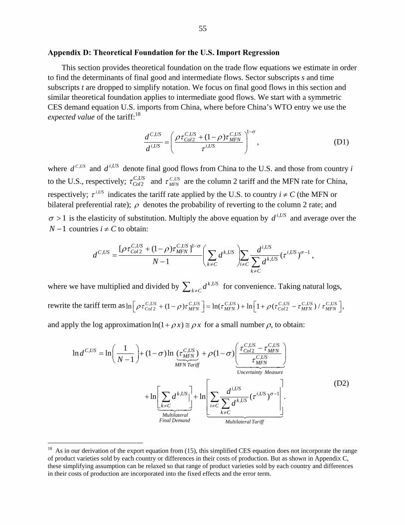
55

Appendix D: Theoretical Foundation for the U.S. Import Regression

This section provides theoretical foundation on the trade flow equations we estimate in order to find the determinants of final good and intermediate flows. Sector subscripts s and time subscripts t are dropped to simplify notation. We focus on final good flows in this section and similar theoretical foundation applies to intermediate good flows. We start with a symmetric CES demand equation U.S. imports from China, where before China’s WTO entry we use the expected value of the tariff:18

1, ,,2

, ,

(1 )C US C USC USCol MFN

i US i US

d

d

, (D1)

where USCd , and ,i USd denote final good flows from China to the U.S. and those from country i

to the U.S., respectively; ,2

C USCol and USC

MFN, are the column 2 tariff and the MFN rate for China,

respectively; USi , indicates the tariff rate applied by the U.S. to country i C (the MFN or bilateral preferential rate); denotes the probability of reverting to the column 2 rate; and

1 is the elasticity of substitution. Multiply the above equation by ,i USd and average over the 1N countries i C to obtain:

, , 1 ,2, , , 1

,

[ (1 ) ]( )

1

C US C US i USCol MFNC US k US i US

k USk C i C

k C

dd d

N d

,

where we have multiplied and divided by ,k USk C

d for convenience. Taking natural logs,

rewrite the tariff term as , , , , , ,2 2ln (1 ) ln( ) ln 1 ( ) / ,C US C US C US C US C US C US

Col MFN MFN Col MFN MFN

and apply the log approximation ln(1 )x x for a small number , to obtain:

, ,, , 2

,

,, , 1

,

1ln ln (1 )ln ( ) (1 )

1

ln ln ( )

C US C USC US C US Col MFN

MFN C USMFNMFN Tariff

Uncertainty Measure

i USk US i US

k USk C i C

k CMultilateralFinal Demand

dN

dd

d

.

Multilateral Tariff

(D2)

18 As in our derivation of the export equation from (15), this simplified CES equation does not incorporate the range of product varieties sold by each country or differences in their costs of production. But as shown in Appendix C, these simplifying assumption can be relaxed so that range of product varieties sold by each country and differences in their costs of production are incorporated into the fixed effects and the error term.

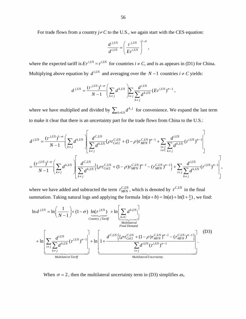
56

For trade flows from a country j C to the U.S., we again start with the CES equation:

1, ,

, ,,

j US j US

i US i US

d

d E

where the expected tariff is ,i USE = ,i US for countries i C, and is as appears in (D1) for China.

Multiplying above equation by ,i USd and averaging over the 1N countries i C yields:

, 1 ,, , , 1

,

( )( )

1

j US i USj US k US i US

k USk j i j

k j

dd d E

N d

,

where we have multiplied and divided by ,k jk US

d for convenience. We expand the last term

to make it clear that there is an uncertainty part for the trade flows from China to the U.S.:

, 1 , ,, , , , 1 , 1

2, ,

, 1 ,, , , 1

2,

( )[ (1 ) ] ( )

1

( )[ (1 ) ] (

1

j US C US i USj US k US C US C US i US

Col MFNk US k USk j i j

i Ck j k j

j US C USk US C US C US

Col MFN MFk USk j

k j

d dd d

N d d

dd

N d

,

, 1 , 1,

) ( ) ,i US

C US i USN k US

i jk j

d

d

where we have added and subtracted the term ,C USMFN , which is denoted by ,C US in the final

summation. Taking natural logs and applying the formula )1ln()ln()ln( ababa , we find:

, , ,

, ,,2, 1

,

1ln ln (1 ) ln( ) ln

1

[ (1 )ln ( ) ln 1

j US j US k US

k CCountry j TariffMultilateral

Final Demand

C US C USi USCol MFi US

k USi j

k j

Multilateral Tariff

d dN

dd

d

, 1 , 1

, , 1

] ( ).

( )

C US C USN MFN

i US i US

i j

MultilateralUncertainty

d

(D3)

When 2 , then the multilateral uncertainty term in (D3) simplifies as,

57

, , , 1 , 1 , , ,2 2

, , 1 , ,

[ (1 ) ] ( )1 1

( ) ( )

C US C US C US C US C US C US C USCol MFN MFN Col MFN

i US i US i US i US

i j i j

d d

d d

.

For convenience, we will use the assumption 2 when we reporting this term in the main text and in the estimating equation (D5), below. When constructing the multilateral tariff term, however, we instead use 6 . We have found that the more complex version of the multilateral uncertainty term, as shown in (D3) for 6 or for other values of , does not perform much differently in the estimation than the simplified version of that term with 2 .

We replace the theoretical coefficients of each variable with regression coefficients to be estimated, including country-pair-sector fixed effects. We also introduce the indicator variable {1995-2000}1 on the uncertainty terms for the years 1995-2000, before China’s WTO entry.

Then from (D2) and (D3) we obtain the equations:

, ( , ), , ,0 1 2

, ,,, 1 2

3 4, ,

ln ln ln

ln ( )

C US C s US C US k USMFN

k CMFN TariffMultilateral

Final Demand

C US C USi USi US Col MFN

k US C USi C MFN

k C

Multilateral Tariff

d d

d

d

{1995-2000},

Uncertainty Measure

1

(D4)

, ( , ), , ,0 1 2

, , ,,, 1 2

3 5,

ln ln ln

( )ln ( ) ln 1

j US j s US j US k US

k jCountry j Tariff

MultilateralFinal Demand

C US C US C USi USi US Col MFN

k USi j

k j

Multilateral Tariff

d d

dd

d

, ,{1995-2000}.

i US i US

i j

MultilateralUncertainty

d

1

(D5)

These two equations are stacked and estimated for merchandise sectors, where we also include traded intermediate goods. In the main text, equations (23) and (24), we add back the time subscript and the sector superscript.

We estimate the probability of reverting to the column 2 rate as the ratio of coefficients for the tariff and the uncertainty measure: from (D2) and (D4), 4 1 4 1/ . In the

first step, is set to one for the multilateral uncertainty term in (D5). In the second step, the

estimated from the first step of (D4) is plugged into the multilateral uncertainty term in (D5),

and we re-estimate the two regressions. We iterate until converges to a certain value, and we

find that only two steps in the iteration leads to convergence.

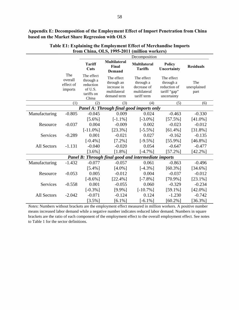
58

Appendix E: Decomposition of the Employment Effect of Import Penetration from China based on the Market Share Regression with OLS

Table E1: Explaining the Employment Effect of Merchandise Imports from China, OLS, 1995-2011 (million workers)

The overall

effect of imports

Decomposition

Tariff Cuts

Multilateral Final

Demand

Multilateral Tariffs

Policy Uncertainty

Residuals

The effect through a reduction of U.S.

tariffs on China


demand term


decrease of multilateral tariff term


reduction of tariff “gap” uncertainty

The unexplained

part

(1) (2) (3) (4) (5) (6)

Panel A: Through final good imports only Manufacturing -0.805 -0.045 0.009 0.024 -0.463 -0.330

[5.6%] [-1.1%] [-3.0%] [57.5%] [41.0%]Resource -0.037 0.004 -0.009 0.002 -0.023 -0.012

[-11.0%] [23.3%] [-5.5%] [61.4%] [31.8%]Services -0.289 0.001 -0.021 0.027 -0.162 -0.135

[-0.4%] [7.2%] [-9.5%] [55.9%] [46.8%]All Sectors -1.131 -0.040 -0.020 0.054 -0.647 -0.477

[3.6%] [1.8%] [-4.7%] [57.2%] [42.2%] Panel B: Through final good and intermediate imports

Manufacturing -1.432 -0.077 -0.057 0.061 -0.863 -0.496 [5.4%] [4.0%] [-4.3%] [60.3%] [34.6%]

Resource -0.053 0.005 -0.012 0.004 -0.037 -0.012 [-8.6%] [22.4%] [-7.8%] [70.9%] [23.1%]

Services -0.558 0.001 -0.055 0.060 -0.329 -0.234 [-0.3%] [9.9%] [-10.7%] [59.1%] [42.0%]

All Sectors -2.042 -0.071 -0.124 0.124 -1.230 -0.742 [3.5%] [6.1%] [-6.1%] [60.2%] [36.3%]

Notes: Numbers without brackets are the employment effect measured in million workers. A positive number means increased labor demand while a negative number indicates reduced labor demand. Numbers in square brackets are the ratio of each component of the employment effect to the overall employment effect. See notes to Table 1 for the sector definitions.

the “china shock”, exports and u.s. employment: a global ... · 4 due to trade, but comparing...

Documents