the circle will now be closed, finally (on the inability...

Journal of Space Operations and Communicator (ISSN 2410-0005)

Volume 12, Issue 2, 2015

The Circle will Now be Closed, Finally

(On the Inability to Adapt Circular Motion to Arbitrary Motions)

E. F. M. Jochim

German Aerospace Centre, Oberpfaffenhofen, Germany

Tel: (+49)-8153-28-2738, Fax: 0-8153-28-1452, e-mail: [email protected]

Summary: The description of the motion of the Sun, Moon, stars, planets and satellites was originally based on a model of circular uniform motion. Improved observational methods re-quired an improved model which was found by superposition of different circles, each trav-ersed by uniform motion. Copernicus seems to have been the first (or at least one of the first) to have recognized that the planets do not move in a circle. The new curve to be adapted to planetary motion was found by Kepler. Based on a general theory of adaptation of any motion as a consequence of the method of the variation of parameters, the present paper shows that the circle is the only curve which is not able to be adapted to any general motion.

Keywords: Circular motion, superposed circular motion, Hansen Ideal coordinates, Hansen system, Leibniz system, Lagrange constraint, method of variation of parameters, general Fre-net formulae, general Darboux vector, system proper motion vector, Fourier expansion

Table of Symbols: Aν Parameters of a curve presented in polar equation form (ν =1,2,3 …– number

of parameter). In the unperturbed case: .A constν ≡

bR, bT, bN acceleration in radial, transversal, normal direction [km/s2]

bRC acceleration [km/s2] of a circular motion

bR0 (radial) acceleration [km/s2] without any physical influence

bRK Keplerian acceleration [km/s2]

qD system proper motion vector of jq -system: jq q jD=D q

G equal area parameter [km2/s]

i inclination [deg]

p semilatus rectum [km]

1



ip Basis vectors of an inertial system (Newton frame) (i=1,2,3)

jq Basis vectors of an ideal system (Hansen frame) (j=1,2,3)

R inertial acceleration vector [km/s2]

,r r state vector: direction vector, absolute velocity vector

0 0 0, ,r q c Basis vectors of co-moving orbit system (Leibniz frame), 0r in radial, 0q in transversal (“transradial”), 0c in normal direction

r radius [km]

t time [s]

u argument of latitude [rad]

V velocity [km/s]

,j jy y Cartesian coordinates in jq -system

δij Kronecker tensor

ζ orbit angle (first Hansen angle) [rad]

η spatial rotation angle (second Hansen angle) [rad]

µ centric gravitational constant [km3/s2]

σ longitude in orbit of ascending node [rad] (related to departure point of Hansen system)

ξ auxiliary angle [rad] for perturbational equations

Ω right ascension (or ecliptical longitude) of ascending node [deg]

1 The Circle as a Model to describe Celestial Motions The idea of the circular motion of the Sun, the Moon and the stars goes back to early Presocra-tian philosophers. Thales of Miletus ( born about 640 BC) assumed a flat Earth disc floating on water and being totally surrounded by water. Therefore the Sun, the Moon and the stars move along an arc which is not specified in detail. However, based on daily observation with respect to the flat surface of the Earth, we may assume that this arc is not necessarily assumed to be a part of a circle, but rather a kind of a highly eccentric ellipse.

Anaximander of Miletus (, ca 610 - 545 BC), a younger contemporary of Tha-les1, is referred to by many as the first philosopher and physicist. His contribution was a scien-tific revolution comparable to the Copernican revolution, possibly being of even greater im-portance. He seems to have been the first to imagine that the Earth, with the shape of a disc, is in suspension in the centre of the universe. Considering this, Anaximander extended the di-mensions of the universe by assuming the diameter to be 56 Earth radii2. The primary matter

1 J. L. E. Dreyer (1953), pp.11-16 2 Other numbers as reported in J. L. E. Dreyer (1953) are not relevant for the topic of the present paper

2



is the “infinite” () which is divided into the four primary elements. These elements are in an eternal battle between the “terrestrial” elements, water and earth, and the “celestial” elements air, and around it, fire. As a consequence, there is a most extensive distance between these groups of elements. Therefore the primary position of fire is like a (circular) wheel at a great distance to the Earth. There are three wheels, one bearing the Sun which is shining through a small opening in the clouds hiding the rest of the wheel, a second wheel inside the Sun bearing the Moon, with a variable opening producing the lunar phases, and inside the Moon a third sphere with a lot of variable openings representing the stars (cf. Figure 1).

0

*

D

RE

E28 R

2/3 RE

Figure 1: Anaximander's view of the universe: the cylindrical Earth body (diameter three times the height) in free suspension, the sphere of the stars (inner circle), the wheel of the Moon (middle), the wheel of the Sun (outer

circle). RE = Radius of Earth = Radius of Earth disc

With this view of the universe, we can conclude that Anaximander introduced the circular motion of the Sun, the Moon and the stars as a physical appearance, and by no means as something that originates in a pseudo-religious superstructure and which would be found in myths.

A more precise modification of Anaximander’s concept was prepared by Pythagoras of Samos (, ca 571 - 497 BC). He assumed the Earth to represent a sphere, which was a very important step forward. He also seems to be the first to introduce the double motion as-tronomy: the daily motion of the stars with respect to the equator, the opposite motion of Sun and Moon with respect to the ecliptic. This is the first further step forward towards the variety of circular motions, the motions in different orbital planes inclined to each other. The deviat-ing motions of the planets were not yet known at that time.

The idea of uniform and circular motion was picked up and continued by Alkmaion of Kroton (, ca 500 BC) a physician who assumed that “all divine beings are always in mo-tion: Moon, Sun, stars, the whole sky”. This is cited by Aristotle3:

3 De anima, A2,405a29pp.

3



Parmenides of Elea ca 515 - 445 BC) assumed that there was a pure celestial air, called “ether”, above which the perfect sphere encloses the finite universe. The stars are af-fixed to this sphere. However, Parmenides assumed that there was no motion of this sphere. There is, of course, no doubt about the circularity of the orbits of the Sun, the Moon and the stars. Platon of Athens BC), deeply influenced by Alkmaion and Par-menides, stressed the term motion in all of his dialogues, especially in the dialogues Timaios and the laws (Nomoi). Platon assumed the motions of the celestial bodies to be of limited life-time (in contrast to Aristotle who assumed eternal life for all these bodies). However, he as-sumed this motion as an image of divine harmony. In contrast to some contemporary assump-tions, Platon required this motion to take place in only one orbit, which is a circle ( ):

„each of them uses the same orbit and not many but always a circle“ 4.

2 The Superposition of Circular Motions N

S

NA

BC

D

e

P8

e

e

Figure 2: left figure: The system of the concentric spheres of Eudoxos of Knidos for the mathematical description of the motion of the planets5: A – Sphere of stars (equatorial system), N = equatorial North pole, S = equatorial

South pole, B – Zodiac (Ecliptical system), e = obliquity of the ecliptic, NE = ecliptical North pole, SE = ecliptical South pole, C and D - spheres to describe the second anomaly of the planetary motion, P = position of a planet (according to the assumed representation of the system of Eudoxos) Right figure: Hippopede (Lemniscate) of

circular geosynchronous satellite orbits in true dimensions: 24h orbit with inclination i = 60°.

4 Nomoi 822a infr. 5 Cf. J. L. E. DREYER (1953), p.90 and F. KRAFFT (1972), p.431

4



Only during the time of Platon was knowledge of the planets propagated in Greece. This new knowledge included the ”anomalous” motion of the planets showing loops and retrograde mo-tions. Although Platon believed this behaviour to be fictitious, he asked the most eminent mathematician of this age, Eudoxos of Knidos (, ca 408 - 355 BC), to describe this motion by mathematical formulation. Eudoxos extended the well known double motion as-tronomy by two additional spheres describing the motion of each of the planets. By this com-bination of two circles on inclined orbital planes traversed with equal velocities, the relative motion with respect to the surface of the Earth will appear as a lemniscate, which was called a “Hippopede” in ancient times. This model still describes the unperturbed motion of a geosyn-chronous satellite moving on an inclined orbital plane at the same speed as the Earth revolves (cf. Figure 2). Here the well known “8” appears, a curve identical with the antique Hippopede. The anomaly described by the model of concentric spheres is known as the “second anomaly”. The “first anomaly”, reflecting the unequal length of the seasons and an eccentric motion of the Sun, was recognized long before Platon. Euktemon (ca 430 BC) observed the periods 93, 90, 90 and 92 days for spring, summer, autumn and winter, respectively. This anomaly was included in Kallippos of Kyzikos' (, ca 330 BC) model of concentric spheres with the assumption of two additional spheres to describe the solar motion. He also introduced an-other two additional spheres for the Moon. Therefore four different spheres, in addition to the spheres related to the equator and the ecliptic, were necessary to describe the motion of the celestial bodies. For the whole solar system he required 33 spheres.

v

3

3

3

3

3

A

S

MaeA

aa

r

Π

O

D

P

d

3

3

MA

A Aσ

3

3

A

S

M

a

ΠO

3

K1

K2

Z

R

3

R3

r

a

D

v3

3

3

R

C

D

PAE

d

rS

A

MAMA

MA

Aσ

Figure 3: Left: Explanation of the eccentric circular motion, S –position of planet, A – apogee, Π - perigee, Md - centre of circular motion, a – radius of eccentric circle, eA – numerical eccentricity, υA – true eccentric anomaly (related to apogee A), MA – mean eccentric anomaly, β - equation of centre (= Prostaphairesis), O – departure

point, P - ascending node of planetary orbit, σ- Longitude of ascending node in orbit, ωA – argument of apogee,

r – Earth-planet distance; Right: explanation of uniform epicyclic motion: R – radius of epicycle = dMD , D – Deferent (=main circle), Z – epicycle, C – centre of epicycle, AE – apogee on epicycle

5



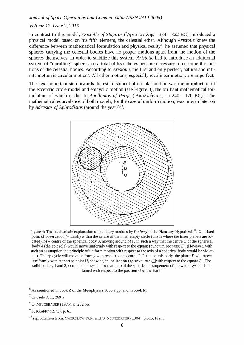
In contrast to this model, Aristotle of Stagiros 384 - 322 BC) introduced a physical model based on his fifth element, the celestial ether. Although Aristotle knew the difference between mathematical formulation and physical reality6, he assumed that physical spheres carrying the celestial bodies have no proper motions apart from the motion of the spheres themselves. In order to stabilize this system, Aristotle had to introduce an additional system of “unrolling” spheres, so a total of 55 spheres became necessary to describe the mo-tions of the celestial bodies. According to Aristotle, the first and only perfect, natural and infi-nite motion is circular motion7. All other motions, especially rectilinear motion, are imperfect.

The next important step towards the establishment of circular motion was the introduction of the eccentric circle model and epicyclic motion (see Figure 3), the brilliant mathematical for-mulation of which is due to Apollonios of Perge (, ca 240 - 170 BC)8. The mathematical equivalence of both models, for the case of uniform motion, was proven later on by Adrastas of Aphrodisias (around the year 0)9.

Figure 4: The mechanistic explanation of planetary motions by Ptolemy in the Planetary Hypothesis10. O – fixed point of observation (= Earth) within the centre of the inner empty circle (this is where the inner planets are lo-cated). M – centre of the spherical body 3, moving around M i , in such a way that the centre C of the spherical body 4 (the epicycle) would move uniformly with respect to the equant (punctum aequans) E . (However, with

such an assumption the principle of uniform motion with respect to the axis of a spherical body would be violat-ed). The epicycle will move uniformly with respect to its centre C. Fixed on this body, the planet P will move uniformly with respect to point H, showing an inclination ( with respect to the equant E . The solid bodies, 1 and 2, complete the system so that in total the spherical arrangement of the whole system is re-

tained with respect to the position O of the Earth.

6 As mentioned in book Z of the Metaphysics 1036 a pp. and in book M 7 de caelo A II, 269 a 8 O. NEUGEBAUER (1975), p. 262 pp. 9 F. KRAFFT (1973), p. 61 10 reproduction from: SWERDLOW, N.M and O. NEUGEBAUER (1984), p.615, Fig. 5

6



Ptolemy (, ca 100 - 178 AD) extended Hipparchos' (130 BC) lunar model by his discovery of the second inequality which, together with the first inequality (the eccentricity of the orbit), is nothing other than a combination of the equation of the centre and the evection. As a new mathematical model to describe this combined motion, Ptolemy used a combination of the eccentric and the epicyclic model. The second of his great discoveries was the introduc-tion of the punctum aequans (the “equant”) as the centre of equal motions: the line connecting the equant with the centre of the epicycle covers equal angles in equal times. Thus the combi-nation of circular motions achieved a new and higher quality. Based on an improvement of the observations (partially prepared by Ptolemy himself), the mathematical description of the ce-lestial motions became increasingly complicated. This was in contradiction to the assumption of Platon that the motion of the celestial bodies were to occur in a very simple manner. Ptol-emy accepted this, thinking that only the mathematical description was complicated, not the physical reality. He wrote11: “It is necessary to always adapt the simplest hypothesis to the motions in the sky. Only if this way is unsuccessful then a more complicated but adaptable hypothesis should be used”. The Almagest, the textbook in Astronomy for about 1500 years, was the first of the great works published by Ptolemy. In the course of his life he tried to im-prove his ideas and published the improvements in astronomy (among them an improved the-ory of the planetary latitudes) in his last work, the “Planetary Hypothesis”. Parts of this work survived but only in its Arabic translation (known by the name kitabal manshurat− ) and was not rediscovered in the west until 196712. In this book, Ptolemy tried to prepare a mechanical model to describe the planetary motions. He assumed that a planetarium could be constructed based on this model (see Figure 4).

3 The End of the Idea of Circular Motion - the End of the Antique Theory of Planetary Motion

There was only little progress in mathematical modelling of orbital motion in the period after Ptolemy. Proclus (AD 412 - 485) derived a mathematical combination of circular and rectilin-ear motion, which was extended by Nasir ad Din at T usi− −

° (died AD 1274), the founder

of the observatory in Maragha in 1259. At T usi−°

’s device improved the theory of plane-

tary latitudes using additional circular motions. He and his students criticized Ptolemy’s phys-ical model with its non-uniform motion of the planets with respect to the Earth and tried to improve the model of planetary motion by introduction of additional epicycles. In this manner, Ibn ash Shatir− (AD 1304 – 1375/76) in Damascus found a model for lunar motion contain-ing a first epicycle representing the equation of the centre and a superposed second epicycle for the evection13. This model, describing lunar motion as a geocentric motion, could be adapted by Copernicus in “de revolutionibus” without any modification. The model of plane-tary motion by Mulaqqad ad Din al Urdi− −' (died AD 1266) and

11 PTOLEMAIOS, Mathematike Syntaxis XIII 2, Teil 2, p.532; included in: Claudii Ptolemaei opera quae exstant omnia, edidit by J. L. HEIBERG, Leipzig 1898-1903; cited in: F. KRAFFT (1973), p.68 12 GOLDSTEIN, B. (1967) 13 ROBERTS, V. (1957)

7



Qutb ad Din ash Shirazi− − (AD 1236-1311) used two epicycles of totally different sizes to describe the motion of the planets. This model was transposed by Copernicus to his heliocen-tric model, erasing one of the epicycles representing the shift from the Earth as the centre, to the Sun as the centre of the motion.

The resulting model was drawn by Copernicus himself in his manuscript de revolutionibus, as shown in Figure 5.

Figure 5: Copy of the facsimile issue of the handwritten original of de revolutionibus (1944), this page including the reference to the non-circularity of the planetary motions and the theory of the (outer) planets based on the

transposition of the planetary model of al Urdi−' and ash Shirazi−

8



The corresponding mathematics is summarized in Figure 6. It shows the coordinates of a planet as presented in an Aphel oriented, planar orbit related, rectangular coordinate system

3 1cos cos cos22 2

1sin sin sin 2 .2

A A A A

A A A A

x r a e a M a e M

y r a M a e M

= = + −

= = −

υ

υ (1)

8

8

8

8

8

M'

F

r1

C1

r2

8

8P

v

A

0

M

M

MM

a

dr

= 0.5 a e

= 1.5 a e

8

8

x

P

P

A

Π

AA

A

A

AyA

rF

Figure 6: The Copernican theory of the motion of the outer planets in their orbital plane: xA, yA – coordinate sys-tem of the orbital plane related to the Aphel PA, PΠ- Perihel, υA = true eccentric anomaly, MA – mean eccentric anomaly, ′Md - centre of the deferent according to al Urdi−' and ash Shirazi− /Copernicus, F – punctum

aequans; motion related to the mean Sun

This is nothing but a Fourier expansion14 of elliptic motion up to the order of accuracy known to Copernicus (about 10 arc minutes or even worse15), therefore a mathematical (and not a

14 KAMLAH, A. (1971); perhaps detected for the first time by G.V. Schiaparelli (see BOCCALETTI, D. AND PUCAC-CO, G. (1996), p.4) 15 Cf. V. BIALAS (1972) and private communication Nov. 2005: the error of Copernicus’s own measurements was in the order of 20 arcminutes, composed by uncertainties in the places of the stars, measurement errors and errors in the mean places of the Sun

9



hypothetical) model of planetary motion based on perfect relevance. The remark of Coperni-cus himself (as shown in Figure 5) seems to be of extreme importance:

“Hinc etiam demonstrabitur, quod sidus hoc motu compositu, non describit circulum perfec-tum iuxta priscorum sententia Mathematicorum, differentia insensibili”

(“in consequence of this composed motion, the star does not describe a perfect circle in ac-cordance to the meaning of previous mathematicians, however, the deviation is negligible”)16.

This sentence includes three interesting statements which must be accepted as recognitions of Copernicus himself:

1. A qualitative statement: the planets do not move in circles. This is the first time in his-tory that, based on mathematical issues, the non-circularity of the orbits of the celestial bodies was accepted. This is also an absolute statement: with mathematical relevance a curve can be a circle or it cannot be a circle (tertium non datur), even if this curve can be represented by superposition of different circles.

2. A quantitative statement: the deviation of the true orbit of the planet’s motion with re-spect to a circular curve is negligible. Lacking accurate measurements, Copernicus had probably no insight into the importance of this statement. It was only three years after Copernicus’ death that an astronomer was born who was able to confirm the consider-ations of Copernicus by means of the incredible accuracy of his naked eye observa-tions of 2 arc minutes and better. Based on these observations, the Fourier expansion (1) had to be extended up to the second order in eccentricity. However, this expansion shows that no more superposed circles could describe the planetary motion.

The author would like to emphasize that the qualitative and the quantitative statements must be regarded independently.

3. A historical statement concerning references to prior mathematicians: Copernicus did not mention any names or origins of these persons. However, we should accept that these people existed and we are quite sure that only (or especially, if among others) the astronomers of Marāgha are meant17.

Based on Tycho Brahe’s (AD 1546 - 1601) excellent observations of the planetary motions, especially of the planet Mars, Johannes Kepler (1571 – 1630) finally stated that no circular motion and also no longer any superposition of circular motions could perfectly describe plan-etary motion. Kepler perceived the ellipse as the curve relevant to all celestial bodies and as-sumed to have found a general law. However, Kepler did not respect precession or any pertur-bations of spherical astronomy, in particular he did not include any mutual influence between the bodies in the solar system, although he supposed a 1/r2 law of force existed between the bodies. I. Newton (1643-1727), who addressed the physical interpretation of the Keplerian motion, was the first to consider the mutual attraction between all celestial bodies based on his law of gravitation. However, only L. Euler (1707-1783) succeeded in establishing a mathe-matical means of solving any problem of motion by his method of the variation of parameters. The basic curve to adapt to any motion is usually a conic section, especially the ellipse in case

16 de revolutionibus 142V10-12. See also SWERDLOW, N. M. und O. NEUGEBAUER (1984), p. 296, n.17. 17 Some scientists will not „believe“ that these astronomers exist. Why should we not believe to that what Coper-nicus himself states?

10



of periodic motions. In 1762, Euler published for the first time the perturbations in elliptic elements, by his method of successive approximation, in his paper „Nouvelle méthode de dé-terminer les dérangemens dans le mouvement des corps célestes, causés par leur action mu-tuelle“18. He described the method of the variation of the parameters in his paper „Considéra-tions sur le Problème des Trois Corps“19, where he also mentioned the orbital elements known today as “Keplerian elements”. It was J. L. Lagrange who derived the general varia-tional equations for the Keplerian elements in case of conservative accelerations, whereas C. F. Gauß extended these equations for the case of non-gravitational accelerations. An im-portant tool to solve these equations was presented by the method of canonical variables by W. R. Hamilton, in the version of H. von Zeipel, and the application by D. Brouwer to solve the main problem of satellite theory.

D

Figure 7: The motion of an equatorial circular body under the influence of J2 only in the pericentre of its osculat-ing ellipse. The right plot shows the values in case of Earth satellites, deviation ∆r[km] versus semi-major axis

a[km]. Geostationary satellites: a0 = 42164.182 km, ∆r = 0.52226 km, oscul. semi-major axis: a = 42166.271 km

In the context of circular motions, a surprising discovery was made by R. H. Lyddane (1963). He was the first to transfer the Brouwer solution from Delaunay elements to a new set of non-singular parameters. In this context, he could show that under the influence of the main zonal effect J2 of a planetocentric gravitational field, a circular orbit of a satellite would be possible only if the satellite were always to be in the pericentre of its orbit, i.e. the argument of pericen-tre and the true anomaly of the orbit are identical (apart from a constant factor) (cf. Figure 7). Let a0, e0, i0 = 0°.0, the Keplerian elements of an unperturbed equatorial orbit, then the oscu-lating radius r of the satellite under the influence of J2 , the semimajor axis a, and the eccen-tricity e will be20

( ) ( )22

2 20 0 2 0 2 0 2 0 2

0 0

1 1 3, , ,2 4 2

E ER Rr r r r J O a B a a r e J O a Ba a

= + ∆ = + + = + ∆ = +

(2)

18 L. EULER collected works, E.398; 8. July 1762 19 L. EULER , Mémoires acad. roy. sci. et belles-lettres 19, 1770, pp.194-220 20 JOCHIM, E. F. AND ECKSTEIN, M. C. (1980)

11



where RE is the mean equatorial radius of the main body and

2

0 0 2 20

3, .2

ERa r B Ja

= =

(3)

Let ω be the argument of pericentre, Ω the longitude (or right ascension) of the ascending node, v the true anomaly, L=v+ω+Ω the true longitude then

( ) ( )22

ddL O Bdt dt

+Ω− =

ω (4)

and, in consequence, the mobile body (Moon, Planet, satellite, orbiter) is moving with the (“unperturbed”) Keplerian mean motion

0 30

naµ

= (5)

staying always in the pericentre of the osculating ellipse with form parameters a and e. For inclined orbits, no circular motion is possible under these conditions. With respect to higher order physical influences, the true orbit will always deviate from circular motion.

4 On a General Theory of Adaptation of any Motion Extending the Eulerian method of the variation of parameters, we come to a more general understanding of the adaptation of any motion, as was first proposed by the antique astrono-mers and more precisely formulated by Ptolemy. Let r be the radius vector of any moving body with respect to a reference point (which is not necessarily a centre of gravitation) and let

0 0 0, ,r q c be the direction vectors of the widely used accompanying trihedron, as was first in-troduced by G. W. Leibniz (1689) into celestial mechanics21, then the variation with respect to time t leads to

0 0 0 0, .r r r= = = +r r r r r r r (6)

Let the value of the variation of the radial unity vector 0r be

0 0 0: , ,ζ ζ= =r r q

(7)

then it can be shown22, that the integral ζ will be the one and only angle of the celestial body related to a Hansen coordinate system. P. A. Hansen (1857 and in previous papers) estab-lished a coordinate system in which “perturbed and unperturbed formulae have identical form”. Hansen called such a system an “ideal” system. In a similar but more generalized sense, he uses the term “ideal” for a behaviour adapting the same form in the perturbed, as well as in the unperturbed, case.

The equations (6) and (7) lead to the orbit normal vector23

21 cf. AITON, E. J. (1960), this system will sometimes be called „orbit system“ in satellite orbital mechanics 22 JOCHIM, E. F. M. (2011/2), theorem 10 and theorem 12 23 The value of the orbit normal vector will be designed with the symbol G according to the corresponding canon-ical element in Ch. Delaunay’s theory and is in this form already widely used in Astrodynamics

12



( )2 20 0 0, 1 .r Gζ= × = = =c r r c c c

(8)

This expression, especially including the general relation

2r Gζ = , (9)

is absolutely independent of any orbital form and corresponds to the initially detected Second Keplerian Law.

Let jq be the basic unit vectors of a Cartesian orbital, plane-related, coordinate system, where q1 is oriented towards a departure point O on the orbit with angular distance ζ to the moving body. Then

( )1 2 0cos sinjjy r rζ ζ= = + =r q q q r (10)

and

.j jj jy y= +r q q (11)

Applying (7), we have

0 ,jjy =q (12)

i.e. the condition for a Hansen system is fulfilled. This system is unvaryingly bound to the (osculating) orbital plane, therefore it is possible to set y3 = 0, so equation (12) leads to

1 2cos sin 0 .ζ + ζ =q q (13)

The system variation vectors jq are usually represented by

j q j= ×q D q (14)

where qD is the system proper motion vector (sometimes misleadingly denoted as “rotational vector”, however, in comparison to the Darboux vector of curvature theory, this vector could also be called “system Darboux vector” or “general Darboux vector” or simply “Darboux vector”). From equations (10) and (13), follow the behaviour of a Hansen system24

q 0× =D r (15)

The consequence is very important: if an integration of the equations of motion takes place in a Hansen system, no proper motion of this system has to be respected because this system is always connected with the motion of the celestial body. An historical dispute between G. W. Leibniz and I. Newton is reflected in this fact: an integration of the equations of motion always has to be executed in a coordinate system whose proper motion vanishes. In his Principia, I. Newton only uses “inertial coordinates”25, i.e. coordinates whose proper motion will be ne-glected. Today, such a system is defined, for example, by the Fundamental Catalogue FK5 and is related to the mean equinox J2000.0. In this context, the equation of motion is

iia= =r R p (16)

24 as found by P. A. Hansen himself in 1857 25 See e.g. in AITON, E. J. (1964): p.32

13



where R is the (inertial) acceleration vector and ai its components with respect to the inertial (=”Fundamental system”) pi (i=1,2,3)26. The correct way to undertake integrations of the mo-tion of planets, and artificial satellites or space probes, is to transform the actual orbital data into this system, perform the integration within this system and afterwards transform the actu-al data back to the true system of date. Based on Leibniz’ co-moving coordinate system with accelerations bR, bT, bN, as used by C. F. Gauß in his perturbation theory, the equation of mo-tion holds

0 0 0 .R T Nb b b= + +r r q c (17)

From equations (6), it follows

0 0 0 02 .r r r rζ ζ ζ= + + +r r q q q

(18)

Introducing the parameters ,ξ η , and because 20 1=q only in the plane perpendicular to q0, the

variational vector

0 0 0: ξ η= +q r c

(19)

will be defined and the acceleration vector becomes

( ) ( )0 0 02 .r r r r rζ ξ ζ ζ ζ η= + + + +r r q c

(20)

Therefore, the transversal acceleration leads to the variational equation for the parameter G based on the transversal acceleration only

TG r b= (21)

and the variational equation for the parameter η based on the normal acceleration only

.Nr bG

η = (22)

According to equation (10), the transversal direction vector in the Hansen coordinate system is written as

0 1 2sin cos= − ζ + ζq q q (23)

and the variation

( )0 1 2 1 2cos sin sin cos .ζ ζ ζ ζ ζ= − + − +q q q q q

(24)

By applying the Hansen property (13), it is known that 1q and 2q are oriented in the identical direction and perpendicular to the plane formed by the basic vectors q1 and q2. Therefore, 1q and 2q have the same direction as 1 2 3 0× = =q q q c . It follows 1 1 0 2 2 0,= =q q c q q c and, including the radial direction vector (10),

( )0 0 1 2 0sin cos .ζ ζ ζ= − − −q r q q c

(25)

Comparison with the variation of the transversal direction vector in equation (19) leads to

26 in Newton’s (et al.) time, the terms force and acceleration were mixed, disregarding Newton’s Second Law of Motion. However, in the era of space flight this should be avoided, also Newton’s Law of Gravitation should not be used as a basis for the equations of motion of a celestial body, e.g. an Earth satellite.

14



0 1 2sin cos .ξ ζ

η ζ ζ= −= − +c q q

(26)

Therefore, equations (17) and (20) lead to the radial acceleration

2Rb r rζ= −

(27)

or the radial acceleration of the moving body

2

3 .RGr br

= + (28)

This equation was found by G.W. Leibniz (1689) in the special case of the Keplerian accelera-tion27

2R RKb brµ

= − (29)

based on the 2-body problem

2 2 2

3 2 3 2 ,G G Grr pr r r

= − = −

µ (30)

where the first notation was derived by Leibniz using the first two Keplerian Laws only, whereas the second notation, including the central gravitational constant µ, includes the 3rd Keplerian Law. Similarly, but independently, I. Newton derived his Law of Gravitation on the basis of the Keplerian Acceleration.

By applying the equations (7) and (19) and the relation 0 0 0= ×c r q , we have 0 0= − ηc q . Therefore. the trihedron 0 0 0, ,r q c will satisfy the system

0 0

0 0 0

0 0 .

ζ

ζ ηη

=

= − += −

r q

q r cc q

(31)

The structure of these equations is comparable to the Frenet formulae of the curvature theory. These formulae similarly represent a co-moving trihedron and could therefore be called “Fre-net formulae of orbital mechanics” (or, particularly, “of Astrodynamics”).

The third equation of system (31) prompts a geometrical interpretation of the parameter η as R. A. Struble performed in 1960: it describes the angular velocity of the rotation of the orbital plane with respect to the instantaneous radius vector (cf. Figure 8). The rotational angle η will be obtained by integration. In fact it is “invisible” because it only becomes visible by its varia-tion. The angle η could be called the „second Hansen angle” if one considers the orbit angle ζ to be called the “first Hansen angle”. However, the variational equation (22) shows a depend-ency of η upon ζ, for which can be derived by applying (9)

27 JOH. KEPLER (1953), Epitome IV, 2, KGW Bd. VII, p.304, also: letter 1. Okt. 1602, KGW XIV,280, line 653-657; see also in HOYER (1976), p.199, U. HOYER (1979), p.71, V. BIALAS (2004) p. 91

15



3

2 .Nd r bd G

=ηζ

(32)

The variation of the rotational angle η is connected with the inclination i, the right ascension of the ascending node Ω, and the longitude σ in the orbital plane by the well-known variation-al equations related to the inertial fundamental system

( ) cos

sin sin ( 0)

cos .i

i u

i u

i

⋅ =

= ≡

=

p

η

Ω η

Ω σ

(33)

8

ζ

c

O

8

8

0

q0

r0

B1B2

r0

SM

Au u+ u∆

i+ i∆i

η

∆η

∆ΩΩ1Ω 2

Figure 8, Left: rotation of the orbital plane around the radius vector with angular velocity η . Right:: detection of the “invisible” angle η in case of normal acceleration of the celestial body at position S

Here u = ζ-σ is the argument of latitude as the node related part of the orbital angle. The an-gle η can be visualized by applying the normal acceleration bN related to an uninfluenced (“unperturbed”) orbital plane with inclination i(0), node Ω(0) and longitude σ(0) of the node. A rotation to the new position of the plane with inclination i(1), node Ω(1) and longitude σ(1) will be according to the spherical triangle e(0), e(1), S with the equations

( ) ( )( ) ( )

( )

(1) (1) (0) (0) (0)

(1) (1) (0) (0)

(1) (0) (0) (0)

cos sin cos sin cos cos sin

sin sin sin sin

cos cos sin sin cos cos .

i i i

i i

i i i

ζ σ ζ σ η η

ζ σ ζ σ

ζ σ η η

− = − +

− = −

= − − +

(34)

Here the parameters i(1), σ(1) are dependent parameters whereas i(0), σ(0) (or Ω(0)) are initial constants related to the uninfluenced orbit. This way, two integrational constants are fixed, the third will be obtained by the integration of equation (21) with respect to the orbital angle ζ

3

,TdG r bd G

=ζ

(35)

The fourth constant will be obtained from the integration of equation (9) in order to get the position of the celestial body against time

16



0

0 2 .Gt t dr

= + ∫ζ

ζ

ζ (36)

The remaining two integrational constants will characterize the curve describing the motion of the celestial body. The polar equation to describe this curve is given by

( ) ( ); ,r r r A= = νζ ζ (37)

where Aν (ν = 1,2,3, … ) are the parameters of this curve. Only two independent parameters are normally needed. With this special curve the real motion should be adopted. This will be treated by selection of a variation of the parameters Aν according to the method of variation of the parameters. If the radial velocity,

dr r r dArdt t A dt

∂ ∂= = +

∂ ∂∑

ν

ν ν

(38)

then for the uninfluenced (“unperturbed”) and the influenced (“perturbed”) motion to coin-cide, the necessary condition will be

.dr rdt t

∂=

∂ (39)

According to P. A. Hansen (1857), this means that the parameters for the adaptation of any motion must be “ideal” parameters. This shows the theory of Hansen in a very interesting new light. Consequently the Lagrange constraint28 holds:

0 or 0 .r dA r dAA dt A d

ν ν

ν νν ν ζ∂ ∂

= =∂ ∂∑ ∑ (40)

If, for example, only two independent parameters have to be considered, then

1 2

1 2

0r dA r dA .A d A d∂ ∂

+ =∂ ∂ζ ζ

(41)

This is the first equation to compute the parameters Aν as a function of the orbital angle ζ (or the time resp.). The second equation will be the (general) Leibniz equation (28)

22

1

.Rdr r r dA G r bd A d r G

ν

ν νζ ζ ζ=

∂ ∂= + = +

∂ ∂∑

(42)

Here, in any case it can be assumed

.r Grζ

∂=

∂

(43)

It remains for the second equation of adaptation

22

1

.Rr dA r b

A d Gν

ν ν ζ=

∂=

∂∑

(44)

28 See e.g. EFROIMSKY, M. (2005)

17



Integration of any orbit using the variational equations above is treated with respect to the Hansen system. In this system the coordinate system proper motion vanishes as in the inertial fundamental system. It is also interesting to see another surprising consequence of the Hansen theory which is that both kinds of orbit integrations take place in a coordinate system with similar properties, even though the basic theoretical structure of these systems is fundamental-ly different.

5 The Inability of the Circle to Adapt any Motion A circle is a curve with the radius as its only parameter. The radius will not vary during a mo-tion on the circle. If A1 = r = const. and A2 = 0 will be set, equation (41) gives

1 1

1

0r dA dAA d d∂

= =∂ ζ ζ

and again, by integration, A1 = r = const. . The Leibniz equation (28) leads to the acceleration of a circular motion 2 3/RCb G r= − whose value is identical to the condition for a uniform rectilinear motion, and so for a circular motion it is 0r = . With mathematical methods there is no chance to escape from the circle. However an escape is possible by physical means. Let bR be any radial acceleration. Related to a circular motion with acceleration bRC, the acceleration “perturbing” the circular motion will be

2

0 3 .R R RC RGb b b br

= − = +

When introduced into the general Leibniz equation (28), the radial acceleration will be

0 ,Rr b=

which ist the acceleration of a motion without any pre-adapted curve. An adaptation based on a circle is not recognizable.

6 Conclusion The theory of the general adaptation of arbitrary motions, which is deducible from Hansen’s coordinate system, has as a necessary consequence the Eulerian method of variation of param-eters in the version of the Lagrange constraint. The unique behaviour of the circle to be una-ble to be adapted to any motion is concluded from this method of adaptation. This shows the uniqueness of the circle among all possible geometrical forms. Adaptation of arbitrary mo-tions using a circle neither helps nor does it harm. Adaptation using a circle is equal to no ad-aptation. If there is no adaptation of any motion it is the same as an adaptation with a circle. Consequently, the circle is worthless in the context of orbital mechanics. (Note: this is a math-ematical issue only, not a physical issue). Therefore the circle is inviolable, it is sacrosanct. An ancient question is answered.

18



Thales of Miletus was not a natural philosopher. As one of the most highly regarded wise men of old, he endeavoured to find simple explanations for the world, however, he knew that „in the simplest things, as the circle, something astonishing and authentic will be contained”29.

Remark: In order to avoid any troubles in reading this paper it should be emphasized that the content is totally restricted to a mathematical representation of the orbits. Of course, by physi-cal-technical means a true circular motion can be controlled, as well as any motion can escape from circular motion. However this physical-technical fact is not subject of the present paper.

7 References AITON, E. J. (1960): 'The Celestial Mechanics of Leibniz', Annals of Science, 16, No. 2, 65–82, (published Au-

gust 1962)

AITON, E. J. (1964): 'The Celestial Mechanics of Leibniz in The Light of Newtonian Criticism', Annals of Sci-ence, 18, 31–41

ARISTOTELES (1983): Vom Himmel, von der Seele, von der Dichtkunst, eingeleitet und neu übertragen von Olof Gigon, Artemis Verlag, Zürich und München

ARISTOTELES (1986): in 23 volumes, Vol. VI On the Heavens, with an English translation by W. K. C. Guthrie, Loeb Classical Library, Cambridge Mass., Harvard University Press, London, William Heinemann Ltd.

ARISTOTELES (1989): in 23 volumes, Vol. XVII Metaphysics I–IX, with an English translation by Hugh Treden-nick, Loeb Classical Library, Cambridge Mass., Harvard University Press, London, William Heinemann Ltd.

BIALAS, V. (1973): 'Die Planetenbeobachtungen des Copernikus. Zur Genauigkeit der Beobachtungen und ihrer Funktion in seinem Weltbild', Philosophia Naturalis. 14, Verlag Anton Hain – Meisenheim/Glan, 1973, Heft 3/4, 328-352

BIALAS, V. (2004): Johannes Kepler, Becksche Reihe Denker, Verlag C. H. Beck oHG, München, ISBN 3 406 51085

BIALAS, V. (2005): Johannes Kepler, private communication

BOCCALETTI, D. AND PUCACCO, G. (1996): Theory of Orbits, Volume 1: Integrable Systems and Non-perturbative Methods, ISBN 3-540-58963-5 Springer Verlag, Berlin Heidelberg NewYork,

BRENSKE, H.-B. (1973): 'Die Entdeckungen des Copernikus, Zur 500. Wiederkehr seines Geburtstages', Sterne u. Weltraum 12, 1973, Heft 2, 36–39

BROUWER, D. AND CLEMENCE, G. M. (1961): Methods of Celestial Mechanics, Academic Press

DICKS, D. R. (1970): Early Greek Astronomy to Aristotle, Cornell University Press, Ithaca, N. Y.

DIELS, N. (1957), Die Fragmente der Vorsokratiker, rowohlts Klassiker Nr.10, Hamburg, pp. 38,39.

DREYER, J. L. E (1953): A History of Astronomy from Thales to Kepler, Dover Publ., New York

EFROIMSKY, M. (2005): 'Gauge Freedom in Orbital Mechanics', Annals of the New York Academy of Sciences, Vol. 1065, New Trends in Astrodynamics and Applications, pp.346-374, Dec. 2005

GOLDSTEIN, B. (1967): 'The Arabic Version of Ptolemy’s Hypothesis', Transactions of the American Philosophi-cal Society. 57, pp. 3-12

HANSEN, P. A. (1857): 'Auseinandersetzung einer zweckmässigen Methode zur Berechnung der absoluten Stö-rungen der Kleinen Planeten, erste Abhandlung', Abhandlungen der mathematisch-physischen Classe der königlich sächsischen Gesellschaft der Wissenschaften, dritter Band, bei S. Hirzel, Leipzig;

29 JAAP MANSFELD (1987), p.42

19


Volume 12, Issue 2, 2015 dritte Abhandlung im fünften Band (1861)

HOYER, U. (1976): 'Über die Unvereinbarkeit der drei Keplerschen Gesetze mit der aristotelischen Mechanik', Centaurus, Vol. 20, 196-209

HOYER, U. (1979): 'Kepler’s Celestial Mechanics', Vistas in Astronomy, Vol. 23, pp. 69-74, Pergamon Press Ltd., Great Britain

JOCHIM, E. F. M. (2011): 'Die Verwendung von Hansen Systemen in Himmelsmechanik und Astrodynamik', German Aerospace Centre, ISRN DLR FB 2011-04

JOCHIM, E. F. M. (2012a) ‘The significance of the Hansen ideal space frame’, Astr. Nachr. / AN 333, No. 8, 774-783 (2012) / DOI 10.1002/asna.202222711

JOCHIM, E. F. M. (2012b): Satellitenbewegung, Band I: Der Bewegungsbegriff [Satellite Motion, Volume I: The Term of Motions], ISSN 1434-8454, ISRN DLR-FB 2012-12, 24. September 2012

JOCHIM, E. F. M. (2012c): Satellitenbewegung, Band II: Bewegung in Raum und Zeit [Satellite Motion, Volume II: Motion in Space and Time], ISSN 1434-8454, ISRN DLR-FB 2012-13, 6. November 2012

JOCHIM, E. F. M. (2013): Satellitenbewegung, Band V: Die Verknüpfung von Bewegung und Beobachtungsgeo-metrie [Satellite Motion, Volume V: The Combination of Motion and Observational Geometry], ISSN 1434-8454, ISRN DLR-FB 2013-12, 26. Juni 2013

JOCHIM, E. F. M. (2014): Satellitenbewegung, Band III: Natürliche und gesteuerte Bewegung [Satellite Motion, Volume III: Natural and Controlled Motion], ISSN 1434-8454, ISRN DLR-FB 2014-36, 28. November 2014

JOCHIM, E. F.; ECKSTEIN, M. C. (1980): 'On the True Circular Orbit of a Satellite'. Celestial Mechanics 21, 1980, pp. 149 – 153

KAMLAH, A. (1971): 'Kepler im Lichte der modernen Wissenschaftstheorie', Philosophia Naturalis. 13, Verlag Anton Hain – Meisenheim/Glan, 1971, 56–73

KEPLER, J. (1953): Epitome Astronomiae Copernicanae, Johannes Kepler, Gesammelte Werke, herausgegeben von Max Caspar, Band VII, C. H. Beck’sche Verlagsbuchhandlung, München, MCMLIII

KOPERNIKUS, N. (1543/1944): Nikolaus Kopernikus Gesamtausgabe, Band 1, Opus de Revolutionibus Coelesti-bus, Manu Propria, Faksimile Wiedergabe, Verlag R. Oldenbourg / München und Berlin

KRAFFT, F. (1971): Geschichte der Naturwissenschaft, Bd. I, ′Die Begründung einer Wissenschaft von der Natur durch die Griechen′, rombach hochschul paperback, Verlag Rombach Freiburg, Verlags Nr. 943

KRAFFT, F. (1972): 'Anaximandros', in: Fassmann, K. (her.), Die Großen der Weltgeschichte, Bd. I, verlegt bei Kindler, Zürich, pp.285-305

LEIBNIZ, G. W. (1689): 'Tentamen de Motuum Coelestium Causis', Acta Eruditorum, Feb 1689, pp. 82-96

LYDDANE, R. H. (1963): 'Small Eccentricities or Inclinations in the Brouwer Theory of the Artificial Satellite', Astronomical Journal 68, 555–558

MANSFELD, J. (1987): Die Vorsokratiker, Griechisch/Deutsch, Auswahl der Fragmente, Übersetzung und Erläute-rungen, Philipp Reclam Jun., Stuttgart

MURRAY, CARL. D. AND DERMOTT, STANLEY, F. (1999): Solar System Dynamics, Cambridge University Press

NEUGEBAUER, O. (1968): 'On the Planetary Theory of Copernicus', Vistas in Astronomy 10, 89–103

NEUGEBAUER, O. (1975): A History of Ancient Mathematical Astronomy, 3 Vol., Springer, Heidelberg

PLATON (1991): Sämtliche Werke, Griechisch und Deutsch, Bände I–X, it 1401–1410, Insel Verlag, Frankfurt am Main und Leipzig

ROBERTS, V. (1957): 'The solar and lunar theory of Ibn ash-Shātīr, a Pre-Copernican Copernican model', Isis 48, 428–432

SALIDA, G. (2004): 'Der schwierige Weg von Ptolemäus zu Kopernikus', Spektrum der Wissenschaft, Sept. 2004, 76-82

SKEMP, J. B. (1942): The Theory of Motion in Plato's Later Dialogues, Cambridge at the University Press

20


Volume 12, Issue 2, 2015 STRUBLE, R. A. (1960): 'The Geometry of the Orbits of Artificial Satellites', North Carolina State College, Ra-

leigh, NC, June 1, 1960; and: Archive for Rational Mechanical Analysis, (1961) 7, 87–104

SWERDLOW, N. M. AND NEUGEBAUER, O. (1984): Mathematical Astronomy in Copernicus's De Revolutionibus, 2 Vol., Studies in the History of Mathematics and Physical Sciences 10, Springer-Verlag, New York, Ber-lin, Heidelberg, Tokyo

The Greek text was written using the TrueType Script Symbol Accentuated by Reinhold Kainhofer (1996)

The Copernicus manuscript was copied thanks to Dr. R. Häfner of the Astronomical Observatory of the Munich Ludwig Maximilian University

Acknowledgments:

The author cordially thanks Mrs. Kerstin Vent, Dr. Burkard Jochim and Mr. Colin Ward for their support in the compilation of this paper.

21

the circle will now be closed, finally (on the inability...

Documents