The Clark Model for Business Cycle Analysiswith Markov Switching Regimes

Master Thesis in Econometrics and Operations Research

31st July 2008

Author: Javier Lopez-de-Lacalle

Supervisor: Siem Jan Koopman

Second supervisor: Soon Yip Wong

– p.1/32

Outline of the presentation

The business cycle. Pioneering works.

The Clark model.

Markov switching models.

The Clark model with Markov switching regimes.

Empirical results.

Conclusions.

– p.2/32

The analysis of the business cycle

Burns & Mitchell (1946)

Business cycles are a type of fluctuation found in the aggregateeconomic activity.

A cycle consists of expansions occurring at about the same time inmany economic activities, followed by [...] recessions, contractions,and revivals.

The duration of the business cycle varies from more than 1 year to10-12 years.

– p.3/32

The analysis of the business cycle

The analysis of the business cycle involves the detection of turningpoints in an economic indicator.

The gross domestic product (GDP) is broadly accepted as ameasure of economic activity.

– p.4/32

The analysis of the business cycle

Beveridge & Nelson (1981)

Devised a procedure for the decomposition of a non-stationary timeseries into a permanent and a transitory component.

Two interpretations of the Beveridge-Nelson (BN) trend:

As an estimate of the trend in an unobserved component model.

As an observed component attached to the definition of anintegrated process.

– p.5/32

The Clark model

Clark (1987)

Upon the framework of structural time series models,

a formal econometric model for the decomposition into a permanentplus a transitory components is specified as:

yt = nt + xt + ut , ut ∼ NID(0, σ2u) ,

nt = gt−1 + nt−1 + vt , vt ∼ NID(0, σ2v) ,

gt = gt−1 + wt , wt ∼ NID(0, σ2w) ,

xt = φ1xt−1 + φ2xt−2 + et , et ∼ NID(0, σ2e) .

– p.6/32

Clark’s model and further stylized facts

In Clark’s model the effect of shocks is symmetric throughout thephases of the cycle.

Further stylized facts observed:

Long and smooth expansion periods alternate with sharp and shortrecession periods.

The amplitude of a recession is correlated with the amplitude of thefollowing expansion.

– p.7/32

Markov switching models

Hamilton (1989) proposed an autoregressive model with switchingmean for the growth rates of the GDP:

yt − µSt=

p∑

l=1

φl(yt−l − µSt−l) + εt , εt ∼ NID(0, σ2) ,

µSt= µ1S1t + µ2S2t ,

where Sjt = 1 if St = j and Sjt = 0 otherwise and St is a first orderMarkov process with transition probabilites:

Pr(St = j|St−1 = i) = pij , i, j = 1, 2 .

– p.8/32

Clark’s model with Markov switching regimes

Asymmetries in the business cycle can be modelled by means of thefollowing variable:

τ = τ0 + τ1St ,

with St = 0 in the first regime and St = 1 in the second regime. St ismodelled as a first order Markov process with transition probabilitiesPr(St = j|St−1 = i) = pij for i, j = 1, 2.

Lam (1990) considers asymmetries in the trend component.

Kim & Nelson (1999) consider asymmetries in the cycle component(Friedman’s plucking model).

– p.9/32

Clark’s model with Markov switching regimes

We implemment a general framework that encompasses previousmodels.

We take a state space representation for Clark’s model.

Asymmetries in the components are modelled as a Markov switchingvariable.

Markov switching parameters are also considered.

The model is estimated by approximate maximum likelihood usingKim’s filtering algorithm.

The general setting is used to explore further versions of the Clarkmodel with Markov switching regimes to address empirical questions inGDP series.

– p.10/32

Empirical results: Switching damping factor

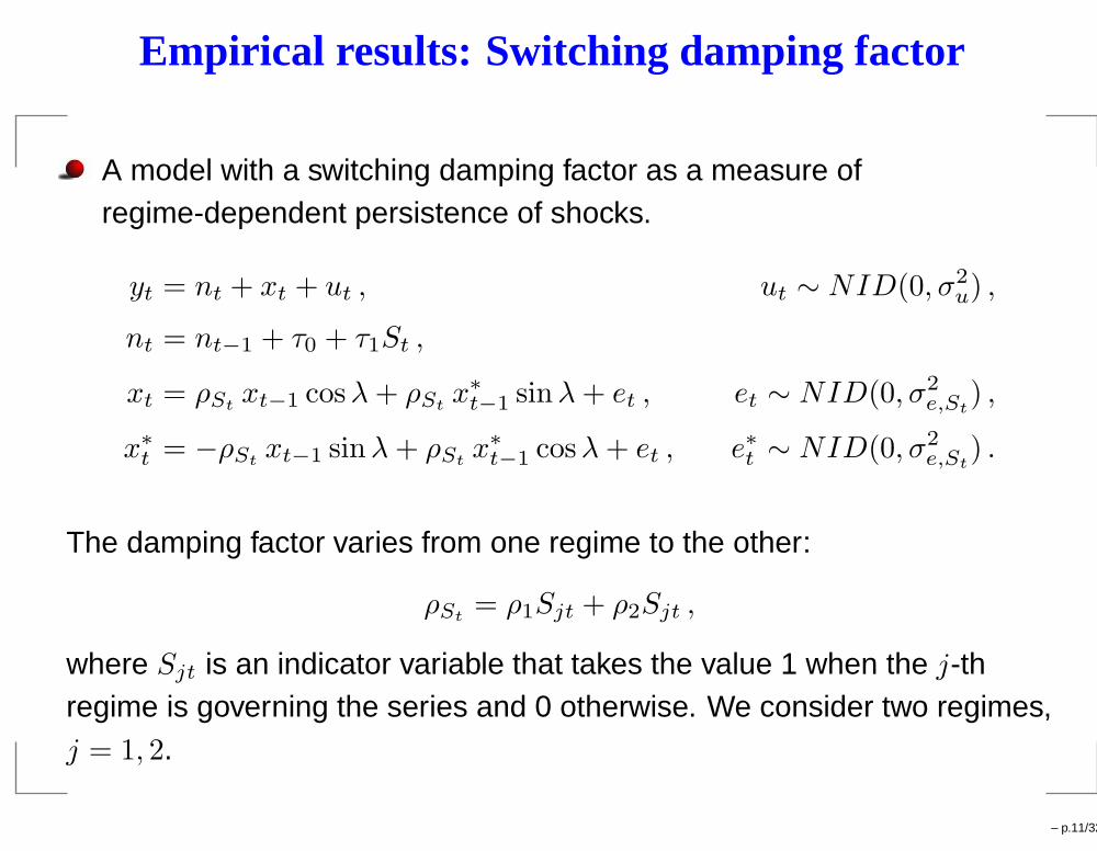
A model with a switching damping factor as a measure ofregime-dependent persistence of shocks.

yt = nt + xt + ut , ut ∼ NID(0, σ2u) ,

nt = nt−1 + τ0 + τ1St ,

xt = ρStxt−1 cosλ + ρSt

x∗

t−1 sinλ + et , et ∼ NID(0, σ2e,St

) ,

x∗

t = −ρStxt−1 sinλ + ρSt

x∗

t−1 cosλ + et , e∗t ∼ NID(0, σ2e,St

) .

The damping factor varies from one regime to the other:

ρSt= ρ1Sjt + ρ2Sjt ,

where Sjt is an indicator variable that takes the value 1 when the j-thregime is governing the series and 0 otherwise. We consider two regimes,j = 1, 2.

– p.11/32

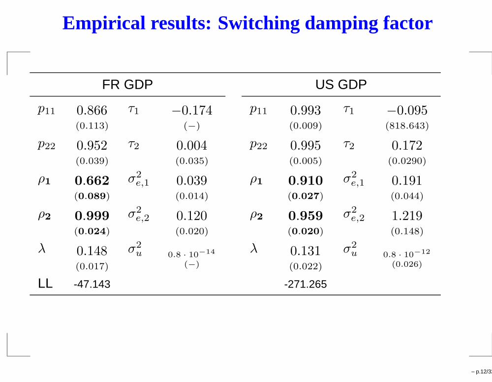
Empirical results: Switching damping factor

FR GDP US GDP

p11 0.866(0.113)

τ1 −0.174(−)

p11 0.993(0.009)

τ1 −0.095(818.643)

p22 0.952(0.039)

τ2 0.004(0.035)

p22 0.995(0.005)

τ2 0.172(0.0290)

ρ1 0.662(0.089)

σ2e,1 0.039

(0.014)

ρ1 0.910(0.027)

σ2e,1 0.191

(0.044)

ρ2 0.999(0.024)

σ2e,2 0.120

(0.020)

ρ2 0.959(0.020)

σ2e,2 1.219

(0.148)

λ 0.148(0.017)

σ2u 0.8 · 10−14

(−)

λ 0.131(0.022)

σ2u 0.8 · 10−12

(0.026)

LL -47.143 -271.265

– p.12/32

Empirical results: Correlated components

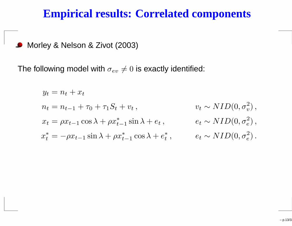
Morley & Nelson & Zivot (2003)

The following model with σev 6= 0 is exactly identified:

yt = nt + xt

nt = nt−1 + τ0 + τ1St + vt , vt ∼ NID(0, σ2v) ,

xt = ρxt−1 cosλ + ρx∗

t−1 sinλ + et , et ∼ NID(0, σ2e) ,

x∗

t = −ρxt−1 sinλ + ρx∗

t−1 cosλ + e∗t , et ∼ NID(0, σ2e) .

– p.13/32

Empirical results: Correlated components

US GDP

p11 0.935(0.030)

p22 0.634(0.120)

τ1 −0.232(−)

τ2 1.789(0.308)

σ2v 3.25 · 10−9

(−)

σ2e 1.454

(1.180)

σev −0.439(0.569)

λ 0.100(0.022)

LL -332.695

– p.14/32

Empirical results: Correlated components

1950 1960 1970 1980 1990 2000

−5

0

5

Inferred cycle

1950 1960 1970 1980 1990 20000.0

0.2

0.4

0.6

0.8

1.0Filtered probabilities of regime 2

– p.15/32

Empirical results: Two transitory components

A model with two transitory components:

yt = nt + xt + ut , ut ∼ NID(0, σ2u) ,

nt = nt−1 + τ0 + τ1St ,

x(1)t = ρ(1)x

(1)t−1 cosλ(1) + ρ(1)x

(1)∗t−1 sinλ(1) + e

(1)t , et ∼ NID(0, σ2 (1)

e ) ,

x(1)∗t = −ρ(1)x

(1)t−1 sin λ(1) + ρ(1)x

(1)∗t−1 cosλ(1) + e

(1)∗t , e

(1)t ∼ NID(0, σ2 (1)

e ) ,

x(2)t = ρ(2)x

(1)t−1 cosλ(2) + ρ(2)x

(2)∗t−1 sinλ(2) + e

(2)t , et ∼ NID(0, σ2 (2)

e ) ,

x(2)∗t = −ρ(2)x

(1)t−1 sin λ(2) + ρ(2)x

(2)∗t−1 cosλ(2) + e

(2)∗t , e

(2)t ∼ NID(0, σ2 (2)

e ) .

– p.16/32

Empirical results: Two transitory components

FR GDP

p11 0.611(0.129)

τ1 −0.423(222.768)

p22 0.913(0.042)

τ2 0.622(0.075)

λ(1)0.298(0.017)

σ(1)e 0.110

(0.030)

λ(2)0.150(0.003)

σ(2)e 0.950 × 10−6

(0.0188)

Log-Lik. 45.406 σu 0.169(0.022)

– p.17/32

Empirical results: Two transitory components

1980 1985 1990 1995 2000 2005

−2

−1

0

1

2

Inferred cycles

1980 1985 1990 1995 2000 20050.0

0.2

0.4

0.6

0.8

1.0Filtered probabilities of regime 1

– p.18/32

Conclusions

In some cases, estimates in a model with changes of regime are inagreement with the understanding of the phases of the business cycle,while in other cases the non-linear model reveals the presence of astructural change or outlier observations.

– p.19/32

Conclusions

The benchmark model discussed in this thesis provides a unifiedframework for the analysis of the business cycle.

The Kim filtering algorithm is shown to be a useful tool for theestimation of a structural model with Markov switching regimes byapproximate maximum likelihood.

– p.20/32

Conclusions

A model with switching damping factor is estimated for the GDP ofFrance and USA. Results for the GDP of France suggest the presenceof lower persistence of shocks in the regime where a lower variance isestimated in the cyclical component.

Correlation between the trend and the cyclical component in a modelwith a switch in the trend is estimated to be negative in the US GDPseries.

The presence of two transitory components is discussed in a modelwith asymmetries in the trend for the GDP of France. A deterministiccycle with periodicity 42 quarters and a stochastic cycle with periodicity21 quarters are detected.

– p.21/32

– p.22/32

Empirical results: Clark’s model

1985 1990 1995 2000 2005−0.03

−0.02

−0.01

0.00

0.01

0.02

Finland

1985 1990 1995 2000 2005

−0.015

−0.010

−0.005

0.000

0.005

0.010

France

1985 1990 1995 2000 2005

−0.002

−0.001

0.000

0.001

0.002

Netherlands

1985 1990 1995 2000 2005

−0.04

−0.02

0.00

0.02

Spain

1960 1970 1980 1990 2000

−0.05

0.00

0.05

United Kingdom

1950 1960 1970 1980 1990 2000

−0.04

−0.02

0.00

0.02

USA

– p.23/32

Empirical results: Markov switching model

UK GDP: AR model with Markov switching variance.

1960 1970 1980 1990 2000 2010

−2

0

2

4

Growth rates

1960 1970 1980 1990 2000 20100.0

0.2

0.4

0.6

0.8

1.0Filtered probability of regime 1

– p.24/32

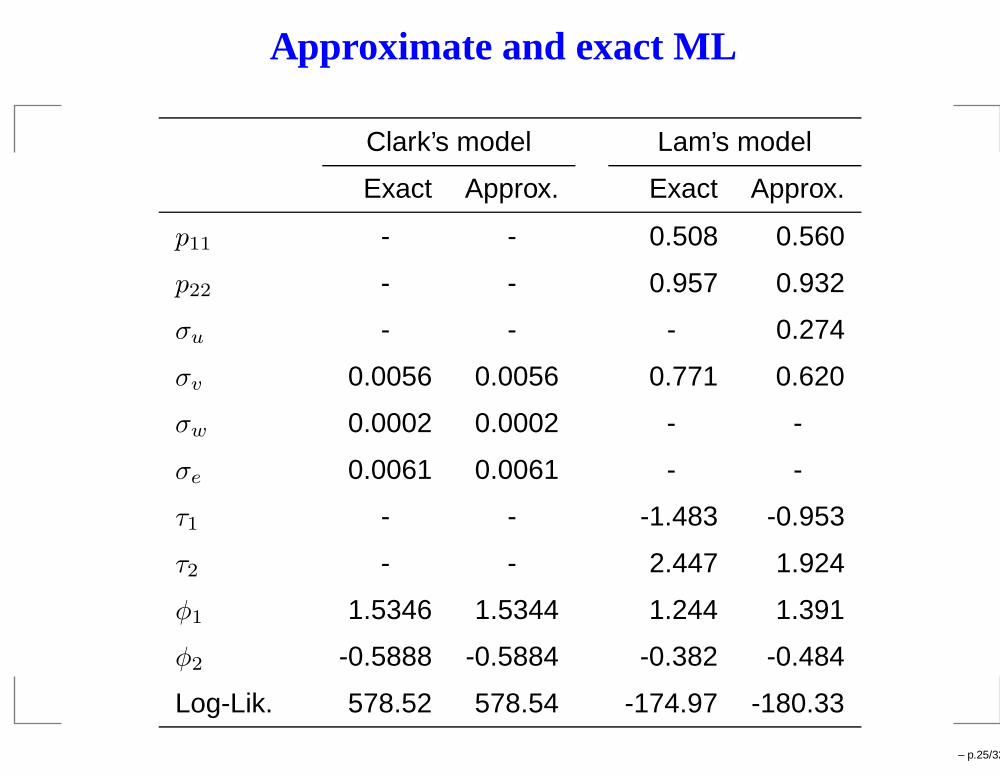
Approximate and exact ML

Clark’s model Lam’s model

Exact Approx. Exact Approx.

p11 - - 0.508 0.560

p22 - - 0.957 0.932

σu - - - 0.274

σv 0.0056 0.0056 0.771 0.620

σw 0.0002 0.0002 - -

σe 0.0061 0.0061 - -

τ1 - - -1.483 -0.953

τ2 - - 2.447 1.924

φ1 1.5346 1.5344 1.244 1.391

φ2 -0.5888 -0.5884 -0.382 -0.484

Log-Lik. 578.52 578.54 -174.97 -180.33

– p.25/32

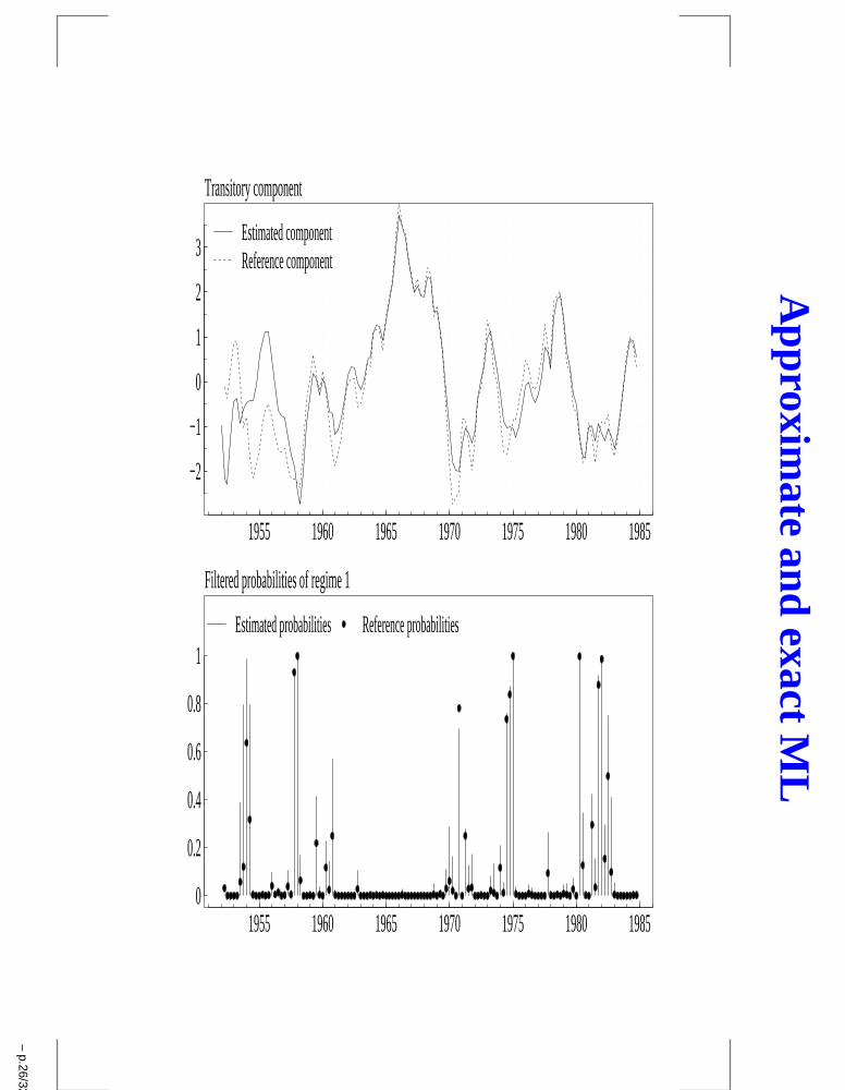
Approxim

ateand

exactM

L

1955 1960 1965 1970 1975 1980 1985

−2

−1

0

1

2

3Estimated componentReference component

Transitory component

1955 1960 1965 1970 1975 1980 19850

0.2

0.4

0.6

0.8

1Estimated probabilities Reference probabilities

Filtered probabilities of regime 1

–p.26/32

State space representation

yt =[

1 0 1 0 · · · 0]

nt

gt

xt

xt−1

...

xt−p+1

+ ut ,

nt

gt

xt

xt−1

...

xt−p+1

=

τSt

0

δSt

0

0

0

+

1 1 0 0 · · · 0

0 1 0 0 · · · 0

0 0 φ1 φ2 · · · φp

0 0 1 0 · · · 0

0 0 0. . . · · · 0

0 0 0 0 1 0

nt−1

gt−1

xt−1

xt−2

...

xt−p

+

vt

wt

et

0...

0

.

– p.27/32

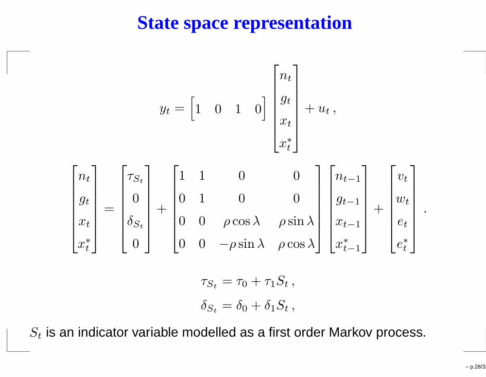
State space representation

yt =[

1 0 1 0]

nt

gt

xt

x∗

t

+ ut ,

nt

gt

xt

x∗

t

=

τSt

0

δSt

0

+

1 1 0 0

0 1 0 0

0 0 ρ cosλ ρ sinλ

0 0 −ρ sinλ ρ cosλ

nt−1

gt−1

xt−1

x∗

t−1

+

vt

wt

et

e∗t

.

τSt= τ0 + τ1St ,

δSt= δ0 + δ1St ,

St is an indicator variable modelled as a first order Markov process.

– p.28/32

ML estimation

1. Run the Kalman filter for all the possible paths of the Markov process in the period t andt− 1, St = j, St−1 = i with i, j = 1, 2, ...,M and M the number of regimes. There areM2 paths to consider leading to M2 state values and variances.

2. Run the Hamilton filter and compute the weighting terms Pr(St, St−1|ψt−1). Thevariable ψt−1 denotes the set of information available up to time t− 1.

3. Collapse the resulting M2 state values and the corresponding variance covariance matrix(for each path St = j, St−1 = i with i, j = 1, 2, ...,M ) into M -vectors according to thefollowing approximations:

α(j)t|t

=

PMi=1 Pr (St = j, St−1 = i|ψt)α

(i,j)t|t

Pr (St = j|ψt),

P(j)t|t

=

PMi=1 Pr (St = j, St−1 = i|ψt)

„

P(i,j)t|t

+“

α(j)t|t

− α(i,j)t|t

” “

α(j)t|t

− α(i,j)t|t

”′«

Pr (St = j|ψt).

– p.29/32

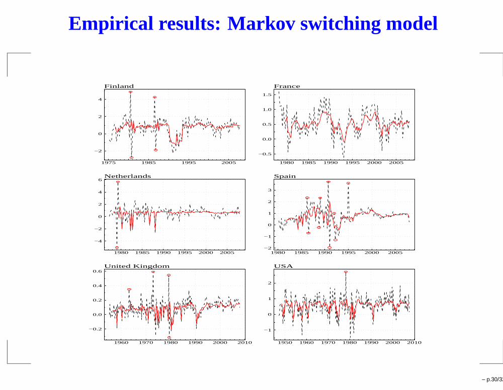
Empirical results: Markov switching model

1975 1985 1995 2005

−2

0

2

4

Finland

1980 1985 1990 1995 2000 2005

−0.5

0.0

0.5

1.0

1.5

France

1980 1985 1990 1995 2000 2005

−4

−2

0

2

4

6Netherlands

1980 1985 1990 1995 2000 2005−2

−1

0

1

2

3

Spain

1960 1970 1980 1990 2000 2010

−0.2

0.0

0.2

0.4

0.6United Kingdom

1950 1960 1970 1980 1990 2000 2010

−1

0

1

2

USA

– p.30/32

Empirical results: Markov switching model

1975 1985 1995 20050.0

0.2

0.4

0.6

0.8

1.0Finland

1980 1985 1990 1995 2000 20050.0

0.2

0.4

0.6

0.8

1.0France

1980 1985 1990 1995 2000 20050.0

0.2

0.4

0.6

0.8

1.0Netherlands

1980 1985 1990 1995 2000 20050.0

0.2

0.4

0.6

0.8

1.0Spain

1960 1970 1980 1990 2000 20100.0

0.2

0.4

0.6

0.8

1.0United Kingdom

1950 1960 1970 1980 1990 2000 20100.0

0.2

0.4

0.6

0.8

1.0USA

– p.31/32

– p.32/32