The College of William and Mary

Honors Thesis

Department of Physics

Investigation of Radiation Detectorswith Silicon Photomultiplier Readout

A thesis submitted in partial fulfillment of the requirements for the degrees of Bachelor

of Science degree in Physics from the College of William and Mary

Author:

Matthew Loftus

Advisor:

Dr. Michael Kordosky

Senior Research Coordinator:

Dr. Henry Krakauer

May 5, 2013

Contents

1 Overview and Background 2

1.1 Purpose . . . . . . . . . . . . . . . . . . . . . . . . . . . . . . . . . . . . 2

1.2 Underlying Mechanisms and Devices: Scintillation and Photo-Detectors 3

1.3 SiPM Performance Studies . . . . . . . . . . . . . . . . . . . . . . . . . . 7

1.4 Physics Motivation: Particle Identification by Time of flight . . . . . . . 9

2 Design and Construction 11

2.1 Test Setup . . . . . . . . . . . . . . . . . . . . . . . . . . . . . . . . . . . 11

3 Performance Studies: Counting Efficiency 15

3.1 Coincidence Rate Measurements . . . . . . . . . . . . . . . . . . . . . . 16

4 The Wavelength Shifter 21

5 Performance Analysis: SiPM/Scintillator Output and Integrated Charge Spectra 28

5.1 Premise . . . . . . . . . . . . . . . . . . . . . . . . . . . . . . . . . . . . 28

5.2 Voltage Traces and Spectra . . . . . . . . . . . . . . . . . . . . . . . . . 29

5.3 Analysis: Taking SiPM Dark Activity(no Scintillator present) into Account 35

6 Radioactive Source Test 37

7 Counter Efficiency: PMT Based Tests 38

7.1 Overview . . . . . . . . . . . . . . . . . . . . . . . . . . . . . . . . . . . 38

7.2 Efficiency: Geometry 1 . . . . . . . . . . . . . . . . . . . . . . . . . . . . 43

7.3 Efficiency: Geometry 2 . . . . . . . . . . . . . . . . . . . . . . . . . . . . 45

7.4 Efficiency: Geometry 3 . . . . . . . . . . . . . . . . . . . . . . . . . . . . 48

8 Conclusions 50

References 53

1

1 Overview and Background

1.1 Purpose

The goal of this project is to investigate how efficiently scintillator radiation detectors

function with silicon photomultiplier(SiPM) based readout. In recent years, faculty and

staff at William and Mary built and assembled the hexagonal scintillator planes and

associated electronics readout for the MINERvA neutrino experiment. The final product

can be seen in figure 1.

Figure 1: MINERvA Scintillator Detector with PMT Readout

The construction of these planes required gluing wavelength shifting fibers into

each piece of scintillator and coupling them individually to a photo-detector know as a

photomultiplier tube(PMT). This process was laborious, and required large input costs.

With our investigation, we sought to determine whether or not this process could be

simplified. More specifically, we wanted to know whether of not we could readout a plas-

tic scintillator directly coupled to an SiPM, without wavelength shifting elements and

complex gluing and coupling procedures. In conducting this study there were many fac-

2

tors we wanted to explore, including what the required size of the SiPM would be, how

efficient were the SiPMs, and how that efficiency would change with the introduction

of wavelength shifting fibers. We also wanted to explore what what role noise played

in SiPM operation, what the single photon sensitivity of the SiPMs was, and how it

depends on the bias voltage.

In addition to their use in large-scale detectors, we also wanted to explore the

viability of using SiPMs to build a application specific detector known as a time of flight

counter. Our primary purpose in building time of flight counters is for particle iden-

tification in low energy test beams(300MeV/c-1000MeV/c). Test beams provide sub

atomic particles of known momentum and identity which are used to calibrate detectors

and detector elements for larger experiments. In characterizing test beams, it is impor-

tant to accurately measure the flux of the different particles that make up the beam.

In other words, experiments must determine what the beam is composed of and how

much of each particle is present. One of the most important performance parameters of

a TOF counter is known as the timing resolution, which is defined by how accurately

the time at which a particle crossed the detector can be determined [9]. With a good

timing resolution, a TOF counter can measure this distribution and give experimen-

talists important data about the performance of their beamline. In many high energy

physics(HEP) experiments, wavelength shifting elements are often used in coupling scin-

tillators to photo-detectors to improve detector performance. As stated before, we would

like to determine how efficient direct coupling is, and whether or not wavelength shifting

elements are necessary in SiPM-Scintillator detectors.

1.2 Underlying Mechanisms and Devices: Scintillation and Photo-Detectors

A typical time of flight counter consists of at least two scintillation devices, each of

which is connected to one or more photo-detectors. Scintillation is a process inherent to

certain organic and inorganic compounds, by which light of a characteristic spectrum

is emitted from the medium following the absorption of radiation. When an energetic

particle travels through the scintillator, it ionizes atoms in the base of the scintillator,

3

freeing electrons. These electrons then excite atoms in the flour component of the

scintillator, causing their electrons to move to a higher energy level. When the electrons

in question return to their original state, the atoms emit photons, and thus particles

passing through the scintillator with enough energy create large amounts of light. The

scintillator we are using was manufactured at Fermilab for the MINOS and MINERvA

experiments, and consists of rectangular extruded polystyrene bars covered in a coating

of titanium dioxide paint, except on the front and back ends. Our scintillator utilized

a polystyrene base, with two flours known as PPO and POPOP, which act to increase

the output light wavelength, shifting it from the ultra-violet to the blue portion of the

electromagnetic spectrum [10].

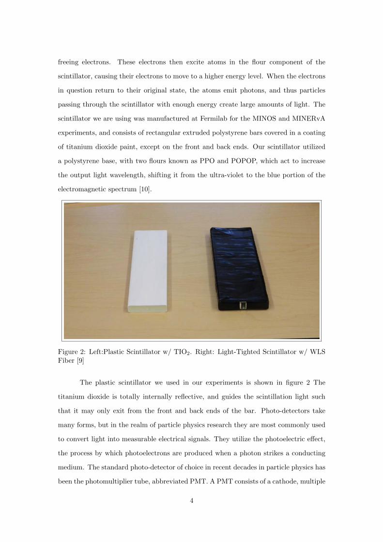
Figure 2: Left:Plastic Scintillator w/ TIO2. Right: Light-Tighted Scintillator w/ WLSFiber [9]

The plastic scintillator we used in our experiments is shown in figure 2 The

titanium dioxide is totally internally reflective, and guides the scintillation light such

that it may only exit from the front and back ends of the bar. Photo-detectors take

many forms, but in the realm of particle physics research they are most commonly used

to convert light into measurable electrical signals. They utilize the photoelectric effect,

the process by which photoelectrons are produced when a photon strikes a conducting

medium. The standard photo-detector of choice in recent decades in particle physics has

been the photomultiplier tube, abbreviated PMT. A PMT consists of a cathode, multiple

4

dynodes, and an anode, all made with conducting materials. A typical PMT-Scintillator

combination is depicted in figure 3.

Figure 3: PMT-Scintillator Detector[5]

A voltage difference is applied between each stage of the PMT, and acts to ac-

celerate electric charges and create an amplification of the electrical signal. When a

photon strikes the photocathode of the PMT, a photoelectron is created, which is accel-

erated through a focusing electrode to the first dynode, where it knocks loose a greater

number of electrons. This amplification process occurs between each dynode until the

signal reaches the anode, contributing to the overall gain of the PMT. The gain of a

photo-detector is the net amplification of the initial input signal. PMTs typically have

a gain of around 106 [9]. From the anode the electrical signal is processed and analyzed,

giving the experimenter valuable information about the original source of radiation. In

detector applications, the cathode of the photo-detector is attached to one of the ends

of the scintillator, so that when energetic particles travel through the scintillator, they

create a light signal that may be recorded by the photo-detector, as shown in figure 3.

In recent years, a new photo-detector, called a silicon photomultiplier(SiPM),

has been introduced with large success. SiPMs have demonstrated an advantage over

PMTs in their size, their required power supplies, in their reaction to magnetic fields,

and in other operational parameters. A SensL 10050 SiPM with a 1mm array and a

5

basic digram showing its parts and operation are shown in figure 4.

Figure 4: Left: SensL SiPM [11]. Right: SiPM Operation Diagram [5]

The mechanisms involved in SiPM operation are slightly different, but the pho-

toelectric effect is still the fundamental element of its operation. SiPMs utilize the

semiconductor silicon, and operate with only one stage of gain. The SiPM array con-

sists of a large number of individual pixels which act in Geiger mode, meaning they are

either on or off. When the light strikes the cathode, which is denoted in figure [5] by ’Si

Resistor’, a photoelectron is released into the silicon substrate. Like the PMT, a voltage

difference is applied between the cathode and the anode, only in this case there are no

dynodes present. At low voltages, the photoelectron will travel from the cathode to the

anode without any amplification. However, when the voltage difference is increased to a

large enough value, known as the breakdown voltage, a process known as avalanche mul-

tiplication occurs. In this process one or more photoelectrons are accelerated to a high

enough velocity that they collide with atoms in the silicon layer, freeing a large number

of electron-hole pairs, which in turn free an even greater number of electron-hole pairs.

Electron-hole pairs refer to a an electron freed from an atomic lattice and the accompa-

nying absence of an electron in the medium. The holes drift toward the cathode where

they are discharged, while the electrons are drawn to the anode, where they provide the

output electrical signal. Silicon is such that one stage of gain provides a comparable

amplification to that of PMTs. Other advantages of SiPMs include their small size, low

operating voltages, and resistance to magnetic fields [5]. For example, the SensL 10050

6

SiPM array we have used for our experiments has a breakdown voltage of 27.5 volts,

while most typical PMTs require 1000 volts or more to function[3]. In detector and

beamline experiments, strong magnetic fields are often present, especially when using

magnetic spectrometers for particle momentum measurements. PMTs’ performance are

greatly impaired by magnetic fields [2], so SiPMs resistance to them provides a very

practical benefit. For these reasons, we chose to investigate SiPMs. This required an

initial analysis of the characteristics of our Sensl SiPMs to familiarize us with their

operation, as all experiments we had previously conducted in light detection utilized

PMTs.

1.3 SiPM Performance Studies

During the summer of 2012, I was able to to perform an in depth study of our SiPM

arrays. We had recently acquired six SiPMs, consisting of three 1mm arrays(10050

model), and three 3mm arrays(30035 model). For our study, we focused on the 1mm

arrays, measuring a number of different parameters. One of the most important param-

eters was the relationship between SiPM gain and the applied bias voltage. To measure

the gain, we had to devise a scheme to determine the overall charge amplification. Not-

ing that the initial charge for a event generated by a single photoelectron is simply that

of an electron, e = 1.6×10−19 Coulombs, we had to find the corresponding charge given

on the scope, and divide it by the elementary charge to get the gain. To do this we

took the integrated charge of the SiPM voltage trace for each oscilloscope trigger, and

recorded the values in a histogram. The voltage traces and the corresponding histogram,

which we will call the integrated charge spectrum, are shown in figure 5.

In the histogram we note the different peaks, which are roughly the integrated

charge values corresponding to single photoelectron events, double photoelectron events,

etc., with the definition of the peaks decreasing as the number of photoelectrons in-

creases. Seeking the charge created by a single photoelectron, we calculated the dif-

ference(V.s) between the 1 P.E. and 2 P.E. peaks, and then divided by the elementary

charge to get the gain. Figure 6 shows our measured relationship between gain and bias

voltage vs. that given by the SiPM datasheet.

7

Figure 5: SiPM Voltage Traces and Integrated Charge Spectra

We note that the datasheet gain relationship is given as a function of the over

voltage, the difference between the current bias voltage and the breakdown voltage. Here

we extrapolated our results to find the bias voltage corresponding to a gain of zero, or

the point at which avalanche breakdown occurs, and found our breakdown voltage to be

27.27 Volts, close to the value of 27.5 Volts given by the datasheet. Another important

note is that our measured gain is approximately two orders of magnitude smaller than

that given by the datasheet. This is indicative of a mistake in our experimental setup

or a real discrepancy between the actual gain of our SiPMs and that given by the

datasheets. We do note, however, that our gain does increase linearly with respect to

our bias voltage, similar to the datasheet behavior.

Further, we studied the following relationships, dark current vs. bias voltage,

dark count rate vs. bias voltage, and dark rate vs. threshold. For all of these studies,

we found for each of the 1mm arrays, their performance agreed with that given by SensL

[11]. With an understanding of the performance of our SiPMs, we determined that they

would be suitable photo-detector candidates for our scintillator radiation detectors. In

8

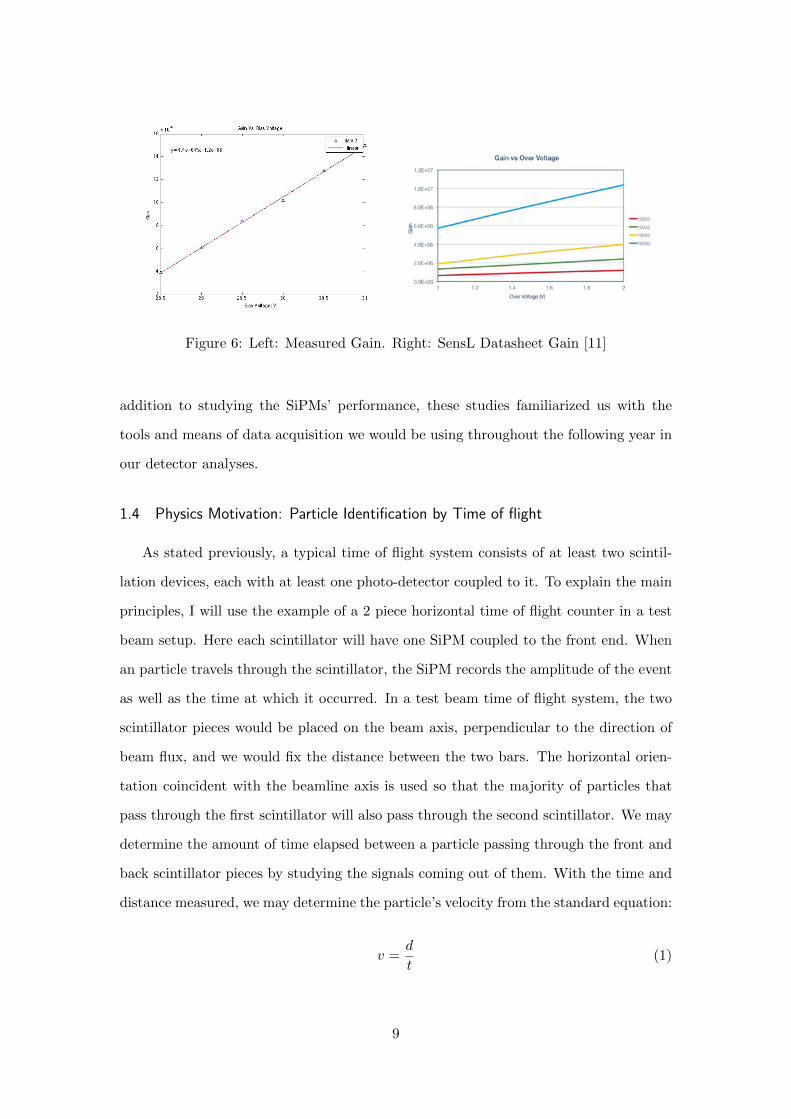
Figure 6: Left: Measured Gain. Right: SensL Datasheet Gain [11]

addition to studying the SiPMs’ performance, these studies familiarized us with the

tools and means of data acquisition we would be using throughout the following year in

our detector analyses.

1.4 Physics Motivation: Particle Identification by Time of flight

As stated previously, a typical time of flight system consists of at least two scintil-

lation devices, each with at least one photo-detector coupled to it. To explain the main

principles, I will use the example of a 2 piece horizontal time of flight counter in a test

beam setup. Here each scintillator will have one SiPM coupled to the front end. When

an particle travels through the scintillator, the SiPM records the amplitude of the event

as well as the time at which it occurred. In a test beam time of flight system, the two

scintillator pieces would be placed on the beam axis, perpendicular to the direction of

beam flux, and we would fix the distance between the two bars. The horizontal orien-

tation coincident with the beamline axis is used so that the majority of particles that

pass through the first scintillator will also pass through the second scintillator. We may

determine the amount of time elapsed between a particle passing through the front and

back scintillator pieces by studying the signals coming out of them. With the time and

distance measured, we may determine the particle’s velocity from the standard equation:

v =d

t(1)

9

In experiments involving test beams, as mentioned above, magnetic spectrome-

ters are utilized independently of TOF counters to measure the momentum of particles in

the beam. The relativistic equation relating the momentum and velocity of fast-moving

particles is:

p = γmv (2)

Where p is the momentum, v the velocity, m the rest mass, and γ the relativistic

constant of the particle in question. Hence with independent measurements of the

momentum and velocity of a particle, we may calculate its rest mass. Noting that

γ = 1√1−( v

c)2

, and plugging equation 1 into equation 2, we come to the following result

m =pt

d√

1− ( dct)

2(3)

Where d is the baseline separation between the two detector elements, c is the

speed of light, and t is the time of flight. The remaining parameters are defined above.

As the masses of most elementary particles are known with reasonable certainty, deter-

mining the rest mass of a particle is the primary means of particle identification. Hence

by measuring the masses of particles in a test beam, we may determine the particle

content.

Figure 7 shows the mass distribution for the test beam used by the MINERvA

neutrino experiment. Here the peaks of the curve correspond to masses of the different

particles present, with the names of the particles listed directly above the x-axis. Here

we see we have a significant flux of pions, kaons, protons, and alpha particles, with pions

and protons accounting for most of the events. A pion is a meson which has a mass

approximately 270 times that of an electron. The width of the peaks is determined by

the timing resolution of the detector elements, with a higher resolution leading to nar-

rower peaks and subsequently more accurate particle distributions. Another plot from

the MINERvA experiment relating particle momentum and time of flight is given in

figure 8 .

Here the different bands correspond to the different particles shown in figure 7.

With a good timing resolution, the bands are narrower and again, knowledge of the

10

Figure 7: Mass Spectrum Example[1]

particle fluxes become more accurate. In our TOF system, the baseline (the separation

between the two detector elements) is always less than half of a meter. Subsequently,

our system is technically a test stand, as it can measure detector performance charac-

teristics but cannot effectively identify particles due to its short baseline and our lack

of an independent system to measure particle momentum. In the following sections, I

will describe the original design of our TOF counter and the subsequent modifications

that took place over the course of the year.

2 Design and Construction

2.1 Test Setup

Figure 9 shows the original schematic for the setup of the detector. When starting

construction, the most important thing to establish was the basic structure of the de-

tector, and to ensure that it had significant flexibility in its design so that modifications

11

Figure 8: Particle Momentum Vs. Time of Flight[1]

could be implemented without needing to alter the major parts of the apparatus. The

most important initial considerations included secure and independent clamping of each

of the elements, the ability to couple and uncouple the scintillator/SiPM without losing

their horizontal and vertical position in relation to each other, and the ability to change

the vertical separation between the two scintillators and lock them in position when

desired. From the initial design in figure 9, we can discuss the structure of the counter.

The original design consists of the two scintillator bars, each coupled to one SiPM/EVB

combination. The EVB is the electrical housing which connects to the anode/cathode of

the SiPM and contains the amplification and voltage biasing circuits. Power is supplied

through a port on the EVB. It also contains the SMA output port which transfers the

SiPM output to an data acquisition system, typically the oscilloscope in our experi-

ments. We note that in the actual experimental setup, there was no air gap between the

end of the scintillator and the face of the SiPM array as is depicted in Figure 9. The

actual experimental apparatus is displayed in figure 10.

12

Fig

ure

9:O

rigi

nal

det

ecto

rd

esig

n

13

Figure 10: First Prototype

For the first build, I constructed the frame using 80-20 stock. I assembled it such

that the two main vertical posts could move back and forth on the two base rails to

ensure precise coupling. Also note the two red handled mechanisms in the foreground

of figure 10, which provided a lockout capability for the two vertical posts when the de-

sired separation was achieved. In addition, the triangular components on inward sides

of the vertical rails, which serve as the detector platforms, had vertical mobility so that

the separation between the two scintillators could be adjusted and locked with relative

ease. Due to the nature of 80-20 and the abundance of compatible accessories, we had

freedom to make changes to the detector, which would prove to be essential in the com-

ing months. Another important aspect of the apparatus is the light tight enclosure our

counter occupancy. This enclosure, referred to as a dark box, serves to prevent ambient

light from reaching the apparatus and adversely affecting the output. When ambient

light hits the array, it creates large amounts of noise and effectively restricts us from

taking any useful data, due to the fact that the SiPM pixels are constantly firing in

14

response to the light.

In assembling the detector, modifications were required, but we were able to

maintain the original structure we had in mind. For this version of the detector, I used

5×1×10cm rectangular polystyrene bars. I attached a highly reflective material to the

back end so that light would reflect towards the SiPM and not escape from the back

end. I used the reflective material on the front end as well, only in this case leaving a

small square of uncoated polystyrene exposed, just large enough cover the face of the

SiPM array. Also, we note the black tape, which in later versions covers the whole

scintillator bar, acting to prevent unwanted light from entering. We currently possess

multiple 1mm and 3mm SiPM arrays, where the dimension corresponds to the length of

the square sides of the silicon/cathode face. However, we also only possess one EVB for

each type of array. This has disadvantages, as the 3mm array has completely different

performance characteristics than the 1mm array, including gain properties and single

photon resolution. Nonetheless, we compensated for these disadvantages in subsequent

experiments by adding an extra stage of amplification to the output of the 3mm SiPM

to match the overall gains of the two detector elements.

3 Performance Studies: Counting Efficiency

To study the performance of our original setup we conducted a measurement of the

coincidence rate between the two scintillator bars. Output voltage studies and inte-

grated charge distributions are very valuable in gauging the efficiency of photo-detector-

scintillator experiments, but at this point our method of coupling was not optimal, so

we did not study these in depth at that stage. With no coupling medium between the

face of the scintillator and that of the SiPM, we experienced significant light loss due

to reflection off of the interface caused by the differences in the indices of refraction of

polystyrene and silicon. Ultimately we acquired Bicron B-600 optical grease, which acts

to match the indices of refraction and minimize light loss, to couple the two components

together. Throughout the rest of the project, we utilized integrated charge spectra and

output voltage amplitudes to determine the effectiveness of our setup. At this stage

15

however, we relied on the coincidence rate measurements for a benchmark of our TOF

counter’s performance.

3.1 Coincidence Rate Measurements

In test beam applications, the two elements of a time of flight counter are often

separated by a distance on the order of meters to gain a useful time differences between

events in the respective scintillators. The minimum separation they can have while still

gaining useful measurements is determined by the timing resolution of the counter. In

our case, however, we kept the distance between the two scintillators less than 20cm.

This was because the size of our light-tight enclosure and 80-20 stock put a low up-

per limit on that separation, but also because coincidence measurements are easier to

perform at a small separation, and yield important information about the efficiency of

the scintillators being used. In calibrating the detector initially, we utilized the abun-

dance of minimum ionizing particles(MIPs) at sea level. MIPs are created in a process

beginning with the reactions of protons and heavier nuclei in the upper atmosphere

as they travel down towards earth. These nuclear interactions create π mesons, which

then decay into muons, particles akin to a heavy electron. While muons have a half life

of 2µs, due to their high velocity and relativistic effects, their lifetime is actually long

compared to other elementary particles. As a result, muons are the primary source of

MIPs at sea level, and a significant proportion of these travel vertically downwards. As

MIPs travel near the speed of light, if they travel through our detector, we expect them

to create events in the two scintillators at essentially the same time, separated by at

most on 1-2 nanoseconds. Also, due to the nature of MIPs, they create large amounts of

scintillation light, hence when an MIP goes through our scintillator we expect multiple

SiPM pixels to be fired, creating a signal with a large amplitude. The thermal electrons

that create the noise are randomly generated in the cathode of a single pixel, hence

the corresponding amplitude has a small amplitude compared to that of MIPs. Thus

we classified coincidences by large amplitude events occurring at nearly the exact same

time. Now for vertical muons of energies greater than 1GeV/c, the intensity at sea level

16

has been experimentally determined to be I = 1muoncm2min2

for horizontal detectors [4]. Thus

taking the vertical cross-sectional area of our scintillator strip and multiplying it by the

intensity given above, we estimate that our scintillator should observe 65 muons/minute,

a rate slightly greater than 1Hz.

To experimentally measure this rate of coincidence in our counter, we used the

NIM electronics units in our lab, which consisted of amplifiers, discriminators, coinci-

dence counters, power supplies, and other DAQ units. Our test setup is shown in figure

11.

Figure 11: Test Setup

In the test setup, we see our dark box located on the left hand side, our oscilloscope

in the center, and our NIM electronics modules on the far right.

In figure 12 we see the NIM electronics setup in greater detail. The individ-

ual modules described above are the rectangular units seen in the figure, with relevant

units places alongside each other for ease and clarity of electrical connections. First,

I connected each of the two SiPMs to to an individual channel on the discriminator

module, which creates a logic pulse of adjustable width each time it receives a signal

above a certain threshold. The thresholds and pulse widths could be set and adjusted

17

Figure 12: NIM Electronics Close-up

for each of the channels on the discriminator, which proves useful for example if one

wanted to set a lower threshold for an input signal which had a lower initial amplifi-

cation compared to other input signals. I then connected the 1mm SiPM to the first

discriminator channel(D1), and the the 3mm SiPM to second discriminator channel(D2).

The two discriminators were then in turn connected to the inputs of a single channel on

the coincidence module. The coincidence module fires a logical pulse each time two

of its inputs are in the logical high state at the same time. Hence if the discriminators

fire at a similar time and their output pulses overlap in the coincidence module, the

coincidence unit will in turn fire a logical pulse. Lastly, I connected the coincidence unit

to an analog counter, which counted the number of coincidences in our scintillators. The

logical elements of our experiment are summarized below.

Based on its logical operations, the coincidence unit can actually measure many

different quantities, including the overall coincidence rate as well as the event rates(Hz)

in each of the scintillators independent of the other. This hinges on the ”and/or” func-

tion of the unit. In the ”and” setting, the unit will only fire a pulse if both inputs go are

low at the same time, so this is what measures the overall coincidence rate. In the ”or”

18

Figure 13: Counting Efficiency: Logical Elements

setting, the unit fires if either one or both of the inputs go low, hence if we disconnect

one of the inputs in this setting, the counter will measure the independent event rate of

the other input.

Each element of the TOF counter will have its own independent event rate,

which means each discriminator output will inevitably be in the ’low’ state for a certain

fraction of each second. The significance of this is that false coincidences will occur,

based on the fact that each element has its own independent rate and the fact that the

NIM units output pulses of nonzero width. To determine these independent rates, let

us take D1, for example. If we multiply the output pulse width of D1 by the event

rate(events per second) coming from D1, we will yield the fraction of each second that

D1 is in the ’low’ state. Now as D1 and D2 both have their own rates, there is a

significant probability that they will both be in the ’low’ state simultaneously, result-

ing in a false coincidence. To measure this quantity I set the NIM unit’s parameters

as follows: Pulse WidthD1= 61.00ns, Pulse WidthD2=64.00ns, ThresholdD1=31.45mV,

ThresholdD2=31.23mV, VBias(1mm)=29.99V, and VBias(3mm)=30.01V. From the above

discussion, we see that we must multiply the fractional time per second one of the dis-

19

criminators is firing times the independent event rate of the other discriminator(and vice

versa), yielding the following formula for the rate of false coincidences per second(in Hz):

Rfc = PWD1 ∗RD1 ∗RD2 (4)

Where Rfc is the false coincidence rate(Hz), PWD1 the width of the output logic pulse

from D1 in seconds, and RD1 , RD2 the independent event rates of D1 and D2, respec-

tively, measured in Hz. Prior to our coincidence test, we measured RD1 , RD2 , finding

RD1 = 6.39 × 104Hz and RD2 = 0.654Hz. Using our false coincidence rate formula, we

calculated the expected value to be Rfc = 2.7 ∗ 10−3Hz. Extrapolating Rfc to find the

expected number of false coincidences in 1 hour yielded a value of 9.72. Extrapolating

our expected rate of muon flux at sea level over the vertical cross-sectional area of our

scintillator(65/min) yielded an expected value of 3900 muons/hour. Subsequently we

performed an overall coincidence measurement over the course of an hour, yielding 10

total coincidences. This indicates a low efficiency. A likely cause was that we may not

have been operating the 3mm SiPM in a sufficiently sensitive way, as indicated by the

extremely low event rate RD2 . After confirming that we were not operating the 3mm

SiPM optimally, we set out to investigate the efficiency in a controlled way. We be-

gan by looking at the photon detection efficiency vs. wavelength characteristics of our

SiPMs. The photon detection efficiency is a measure of how well input light is converted

into an electrical signal, as well as what proportion of that light is detected. Figure

14 shows the photon detection efficiency, for a number of different SensL SiPMs, where

the performance of our 10050 SiPM array is given by the yellow curve. We see from

the figure that the maximum PDE occurs at approximately 500nm, meaning the most

efficient signal amplification occurs when light with λ = 500nm strikes the cathode. At

this value the PDE is slightly greater than 20 percent.

Our polystyrene scintillator’s output characteristics and some related quantities

are shown in figure 15. The 1%PPO+0.03%POPOP transmittance, given by the blue

curve, shows the wavelength of the light created within our scintillator. Note PPO and

POPOP are the dopants used in the polystyrene to create the scintillation mechanism.

The curve shows that most of the scintillator’s output light has a wavelength between

20

Figure 14: SensL SiPM PDE Characteristics [11]

400-420nm. Referring back to figure 5, we see that the 400-420nm region corresponds

to a PDE of 5% or less, much lower than the maximum PDE for the 10050 SiPM.

So the two media are not well matched optically, and much of the scintillator light is

transmitted inefficiently. With a better optical coupling, we would ideally get a much

higher signal amplitude for MIP events in our scintillator, thus allowing us to raise the

thresholds and better discern between noise and actual particle detection events. This

finding led us to our next modification of the detector.

4 The Wavelength Shifter

Our previous results motivated us to construct a device which would shift the wave-

length of our scintillator output to a wavelength more suitable for our SiPMs. In figure

15, we see the red curve corresponding to K27 transmittance. K27 is the dopant found

in the green WLS fibers, which have been utilized in combination with scintillators and

photo-detectors in the MINOS and MINERvA neutrino experiments, as well as other

particle physics experiments. K27 is used to shift scintillator light to a higher wave-

length. As shown in the figure, it primarily emits light with a wavelength between

21

Figure 15: Polystyrene and K27 Dopant Transmittance Characteristics[3]

470-500nm, which corresponds to a much higher PDE in our SiPMs, hence if utilized

properly it would serve as a suitable solution to our optical matching. In our lab, we had

large stock of 1mm and 1.2mm diameter green WLS fibers. Using these fibers, we de-

vised a plan to make a connector between our scintillator and the face of our SiPM array,

thus shifting the wavelength accordingly. Figure 16 below depicts the basic structure

of the wavelength shifter. On the left hand side we have the EVB/SiPM combination.

To the right of that we have a component which connects the face of the SiPM to the

face of the main shifter component. To the right of that, we have the third component,

which couples the main shifter component to the front end of the scintillator, which is

seen on the far right.

22

Fig

ure

16:

Wav

elen

gth

Sh

ifte

rO

verv

iew

23

Figure 17 shows each of the connector components in much greater depth with

accurate dimensions. We note the 9 circular holes in the device on the left hand side.

This is the component of the shifter where the ultra-violet light is absorbed and re-

emitted in the green portion of the EM spectrum, performing the main function of the

connector. Here 9 WLS fibers, each 30mm in length, are strung through the connector

and each one secured in place using epoxy resin. Our fibers were initially over a meter

long, so we had to find an efficient method of cutting them and polishing such that we

would not significantly reduce the transmission. To do this, I initially cut the fibers

with a razor blade, but this created cracks in the fibers, damaging their output and

rendering them useless. To solve this and ensure the fibers maintained their integrity, I

heated the razor blade for approximately 20 seconds with a propane torch, immediately

before cutting. Using the heated blade I was able to cut through the fibers without

creating any cracks. After cutting, I coated each of the fibers in epoxy resin and strung

them them through the connector individually until all 9 were in place. After letting

the epoxy cure for 24 hours, I proceeded to cut the excess fiber ends off of each side of

the connector, again with a heated razor blade. I then polished each end slowly using

a series of fine grit polishing sheets. Using a progressively higher grit each time, I was

able to achieve a smooth finish, where each side had a high degree of transparency and

minimal surface scratching, as viewed through a magnifying lens. The other portions

of figure 17 depict the front-end and back-end parts of the connector, respectively. The

dimensions of these components had to be accurate to a single millimeter for the correct

faces to align and to ensure that the enclosure was still light-tight.

I worked in collaboration with machine shop technicians, and had them fabricate

all of the individual pieces. We had to make a number of changes and iterations of the

initial design based on the precision and types of equipment available for metalworking.

I have summarized the necessary modifications in figures 18 and 19.

24

Fig

ure

17:

Sm

alle

rco

mp

onen

tsin

dep

th

25

Figure 18: Main wavelength shifting component redesign

Ultimately, the final design was significantly different component-wise than the

original, but all of our original specifications and functions were still met. The procedure

of putting the actual connector together involved a slow process of binding each metal

piece together with epoxy, allowing it to cure, then proceeding to bind those components

together and repeating the process until the apparatus was complete. Once the appara-

tus was in one solid piece, I applied RTV caulk to the gaps and locations where different

components met to ensure it was light-tight. In regards to the scintillator, I applied 3

coats of titanium-dioxide paint to the clear surfaces of the polystyrene, leaving exposed

only the roughly 3mm×3mm square meant to mate with the end of the fiber-optic con-

nector. On top of this layer of paint I added an additional layer of the reflective sheet

mentioned previously, to ensure no light escaped from the back end or the non-couple

portion of the front end. To actually join the two surfaces, I applied a thin film of Bicron

BC-630 optical grease to the end of each face(to minimize reflection losses), inserted the

scintillator into the slot lined up with the fiber-optic face, and sealed them with RTV

26

Figure 19: SiPM/Shifter side connector

caulk. For the connector on the opposing end, I used a 4-lead rectangular connector to

extend the leads of the SiPM. I then inserted the SiPM into the connector, such that

its face was flush against the fiber-optic connector, again using the same technique of

applying a thin layer of optical grease at the interface between the two. Lastly I sealed

the front end portion with RTV, and placed the assembled shifter in the braces of the

TOF counter. The final product in its 80-20 mounting apparatus in the dark box is

shown in figure 20.

27

Figure 20: Scintillator/SiPM pair with wavelength shifting connector

5 Performance Analysis: SiPM/Scintillator Output and Integrated Charge

Spectra

5.1 Premise

Following the construction of our wavelength shifter, we needed to develop a method

to study the performance of our different SiPM/Scintillator coupling methods and de-

termine which would yield the best performance in our time of flight counter. The

four cases we had were SiPM with no scintillator, SiPM/scintillator directly coupled

(surface-to-surface), SiPM/scintillator with optical grease at the interface, and lastly

our wavelength shifter coupling. To study each of the methods, we decided to com-

pare them with the output of the SiPM on its own. Observing the voltage traces and

corresponding amplitudes was useful, but as the pulses lasted typically over 100ns, the

amplitude was not completely informative of the SiPMs output. To take this into ac-

count, we also integrated each voltage trace and recorded the values in a histogram to

28

get a spectrum of integrated charges, yielding a more complete understanding of the

events in our detector. We note that here we were studying the performance of a single

counter, as opposed to our coincidence rate tests, which involved the use of a pair of

counters. Hence for each case, we set up one scintillator with the appropriate coupling

method and recorded the results.

5.2 Voltage Traces and Spectra

Using our 1mm 10050 SiPM array, with the voltage bias set to 30.05 Volts, we

took the following traces. In our voltage traces, we set the scope persistence parameter

to 20 seconds, which means the scope displayed all of the traces that had been taken

in the previous 20 seconds, beneath the most recent trace. This setting is valuable

because it allows us to distinguish the peaks corresponding to the the number of incident

photoelectrons and study the general behavior over time, rather than studying each

individual pulse. Significant outliers may not appear in the final scope trace, but their

values are recorded into the integrated charge histogram. Also, we set the scope to

trigger on signals less than or equal to -10mV, on the negative edge of those signals.

Figure 21: SiPM w/out Scintillator Voltage Output

29

In figure 21 we see our 1 P.E., 2 P.E., etc. peaks well defined on the trace, with

blue lines surrounded by a purple background. The different peaks correspond to the

number of photoelectrons generated in the SiPM for a single event. More energetic

events, MIPs for example, can create multiple photoelectron pulses. As a MIP can

create more scintillation light, it may cause a higher number of pixels in the SiPM array

to fire. When multiple pixels fire, we get a larger signal amplitude above the 1 P.E.

level. Here the highest common events appeared to take place at the -80mV level.

Figure 22: SiPM w/out Scintillator Integrated Charge Spectrum

In figure 22 we see the peaks corresponding the number of incident photoelec-

trons, as observed in the voltage traces. These peaks are well defined, with 1 p.e.

∼-2.8nVs, 2 p.e. ∼-2.96nVs, and 3 p.e. ∼-5.18nVs.

30

Figure 23: SiPM/Scintillator Direct Couple Voltage Output

From figure 23 we see the photo electron peaks well-defined. For the most part

the highest common events were again at ≈ -80mV, however we do see some events in

the 100mV range. We note that the persistence setting on the voltage traces causes

them to display all the traces of the previous 20 seconds, and automatically deletes the

traces prior to that. This setting is constantly running on the scope, so we are always

seeing what has occurred in the last 20 seconds. Hence the high amplitudes of some of

the pulses in figure 23 could simply be due to the random occurrence of events and the

particular 20 second time interval the scope was displaying.

31

Figure 24: SiPM/Scintillator Direct Couple Integrated Charge Spectrum

We see from figure 24 the P.E. peaks are less defined, with more events having

integrated charge values between the levels at which the P.E. peaks occur. However, we

note that the scale of this histogram is larger, and thus the bin value as well, than the

previous histogram. Hence the lack of definition is likely due to the fact that we are

viewing a horizontally ’compressed’ version of the histogram in figure 22.

Figure 25: SiPM/Scintillator Optical Grease Voltage Output

32

For the optical grease coupling, the voltage trace results were quite similar to the

those of the first two cases, with the peaks well defined, as shown in figure 25.

Figure 26: SiPM/Scintillator Optical Grease Integrated Charge Spectrum

For the optical grease coupling, the integrated charge spectrum, shown in figure

26 was very similar to that of the direct-couple case, with the P.E. peaks not clearly

defined.

Figure 27: SiPM/Scintillator Wavelength Shifter Voltage Output

33

For the wavelength shifter case, the voltage amplitudes were in a similar range

as those of the first three cases, however the P.E. peaks are not as clearly defined in

the voltage scope trace as in the other cases. Also, there is an extra element of noise

in the voltage traces, causing most of the individual signals the jitter up and down over

the course of each acquisition. This could be due to the wires used to couple the SiPM

to the EVB. We note that in the wavelength shifter, as we connected the SiPM leads

into a rectangular connector, we had to insert two more leads on the opposite side in

order to couple the SiPM to the EVB. The EVB contacts for the SiPM, however, are

thinner than most common single strand wire. As a result of this I was forced to unravel

multi-strand wires, clip off unwanted strands, then recoil them to produce wires with a

diameter small enough to fit the EVB. The termination of these individual strands may

have let to reflections and other deficiencies which contributed to the noise.

Figure 28: SiPM/Scintillator Wavelength Shifter Integrated Charge Spectrum

From figure 28, we see the integrated charge spectrum was similar to that of the

direct-couple and optical grease cases, again with the P.E. peaks not well-defined. From

this analysis of the different coupling methods we were able to see that they all shared

similar voltage output amplitudes, and we were able to discern the different P.E. peak

resolutions from the integrated charge spectra. This visual inspection was useful, but it

did not lead us to applicable results about the different coupling methods.

34

5.3 Analysis: Taking SiPM Dark Activity(no Scintillator present) into Account

To gain useful data about our different coupling methods, we needed a procedure

to separate the data produced by the SiPM independent of the coupling method, from

the data which was actually due to the presence of the scintillator. In other words

we wanted to know how many events were actually caused by the scintillator, and

what those events were like. From the scope, we were able to take the histogram data

(bin location(V.s) and bin population(#events)), and export it to a spreadsheet. Now

as the SiPM produces negative output voltages, the more negative integrated charge

values actually correspond to the more energetic events. What we wanted was a way to

measure the occurrence of high level events in the SiPM benchmark case, and compare

it to that of the other coupling methods. To do this we created a plot where the x-axis

value corresponds to the integrated charge value, whereas the y-axis value corresponds

to the percentage of the total events that had an integrated charge value less than the

current x value. Hence for each integrated charge value, it would show what proportion

of the total events had a higher (absolute) integrated charge than that value. In our

tests we set the voltage bias to 30.58 Volts, and ran the histogram function for 5 minutes

for each of the coupling methods. Also we set the threshold of the oscilloscope trigger

to -20mV up from -10mV. This was out of concern for the effects of noise and low level

events on the operation of the oscilloscope. The scope has an inherent dead time after a

trigger occurs in which it cannot acquire data. Our concern was that at a threshold of

-10mV, we would experience an extremely large quantity of low amplitude events, and

thus more total dead time, hindering our ability to detect the high amplitude events we

were looking for.

The plot of figure 29 gives the percentage relationship described above. We note

the general trend of the plot; that the proportion of total events with a higher magni-

tude decreases as the integrated charge decreases. In this case, we were interested in

using the 1% level as a benchmark. Though the plots detail does not show the precise

location of the 1% mark, our data showed that it occurred at −2.45 ∗ 10−8Vs, and that

there were 94 total events with an integrated charge greater than −2.45 ∗ 10−8Vs. In

the absence of high amplitude noise, if we subtract the number of high level events in

35

Figure 29: SiPM w/out Scintillator Percentage Plot

the SiPM benchmark case from that in one of our scintillator coupling cases, we would

yield the number of true MIP events. Hence taking similar histograms for the three

coupling methods, we yielded the following values. For the direct-couple, we yielded 111

events of magnitude greater than −2.45 ∗ 10−8Vs, which gives us 17 real MIP events.

Now for the other cases, though, we found zero events above the −2.45 ∗ 10−8Vs level.

Taking into account our previously mentioned vertical MIP rate of 65 muons/minute,

we would expect 325 muons to pass through our scintillator in 5 minutes. Now we

know the histogram function has a limit on the percentage of events it can record, so

we would not expect to see all of those events. Even so, the number of high level events

we detected was a surprise, perhaps resulting from our coupling methods, or from our

data acquisition methods and the instruments used, which may not have been optimally

suited to record cosmic events.

We repeated a similar test the following week, extending some of the parameters

to gain a better understanding of the underlying issues. We set the voltage bias to 29.5

Volts, which is the recommended operating voltage given by the SensL data sheet. We

36

also kept the trigger level at -20mV. For this test, we ran each case for 20 min to increase

the number of total events and thus the corresponding error. Also, instead of just using

the 1% level, we looked at events above the 1.1%, 5.3%, 11.2%, 21.6%, and the 47.2%

levels, to see if the behavior we observed in the last test extended to the entire integrated

charge spectrum. We chose those decimal values because of the discrete nature of the

bin location given by the scope, i.e. because we are unable to find the number of events

for an integrated charge value located between two bins. Ultimately, we found for each

coupling method, for each percentage value just mentioned, the number of events was

less than that of the SiPM benchmark case. This showed that in the dark box, with no

additional light source, the integrated charge spectra for each of the different coupling

methods had a smaller magnitude than that of the SiPM benchmark case. This did not

make sense, and led us to seek new means of studying the scintillators responsiveness

to light.

6 Radioactive Source Test

In light of the problems we faced with our different coupling methods and detecting

MIP events, we wanted to test the scintillator with an energetic source of charged

particles to ensure that it was in fact working and that the scintillator was increasing

the output voltages detected by our SiPM. We also wanted to observe whether or not

the counting rate of the SiPM increased with the introduction of a radioactive source.

For this we used a Cobalt-60 radioactive pellet. The Co-60 is a Beta emitter, which

emits photons of 1.173MeV and 1.333MeV [9]. In this test we coupled the scintillator

to the 10050 SiPM with optical grease, set the trigger to -20mV, and ran the histogram

for 20 minutes so that we could compare the integrated charge spectrum to that of the

optical grease coupling case from the previous experiment.

Figure 30 depicts the number of total events above each particular integrated

charge value with and without the radiation source present. The difference between the

two curves shows the total number of events that we can attribute to the presence of the

Co-60 source. We saw that a radiation source did in fact yield more high-level events,

37

Figure 30: Radioactive Source Test Results

and that the integrated charge spectra of our SiPM/Scintillator combination increased.

This result was valuable, as it showed that our system was responsive to radiation.

7 Counter Efficiency: PMT Based Tests

7.1 Overview

With an understanding of how our different coupling methods and varying amounts

of radiation affected the output of our system, we sought to find a new measure of the

efficiency of our counter, in this case relative to a pair of preexisting counter known to

be operational. For this we used two photomultiplier tubes, each coupled to a scintilla-

tor/light guide combination, with the light guide acting to direct the scintillation light

to the photocathode of the PMT. Figure 31 shows the structure of our initial test setup

for our efficiency measurements.

In figure 31, the two cylindrical objects are the PMT housings, which contain

the voltage biasing elements as well as the PMTs themselves. On the right hand side of

38

Figure 31: Initial Efficiency Test Setup

the PMT housings, we see a smaller black cylindrical object followed by a rectangular

object. The cylindrical objects are the light guides, while the rectangular pieces are

the scintillators. In between the two PMT elements we see another rectangular piece of

scintillator coupled to a green circuit board, both secured with the vertical clamps. This

is the SiPM-scintillator counter element whose efficiency we are studying. The idea is

based on the nature of vertical muons. If a muon traveling downwards strikes both PMT

based counters, it must inevitably travel through the SiPM based counter in between

the two. The way we measure the efficiency is to count the number of coincidences in

the two PMT based counters and compare it to the number of coincidences we get in all

three counters. We will refer to a coincidence in the two PMTs as a double coincidence,

and a coincidence in the two PMTs and the SiPM as a triple coincidence.

Figure 32 shows a typical double coincidence from one of our subsequent tests. In

the oscilloscope trace, we see the three different traces corresponding to channels 1,2

and 3. Here PMT 1 is the yellow trace on channel 1, PMT 2 is the pink trace shown

on channel 2, and the SiPM is the dark blue trace shown on channel 3. The light blue

39

Figure 32: Typical Double Coincidence

histogram at the bottom records the integrated charge of the SiPM trace taken at each

trigger of the scope. Noting that each horizontal division corresponds to 50ns, we see

in this example that PMT 1 and PMT 2 received strong signals at essentially the same

time, while the SiPM output no signal. An important aspect to note of these tests was

the special pattern on which we triggered our oscilloscope. Here we would get a scope

trigger each time CH1(PMT 1), and CH2(PMT 2) went below -50.0mV at the same time,

regardless of amplitude of the SiPM signal. We see the results of this in the histogram

in the bottom of figure 32, where 2 large PMT signals and no SiPM signal resulted in

histogram values in the ’No Signal’ region, while triple coincidences with large SiPM

signal amplitudes resulted in large histogram values in the ’Large Signals’ region. The

significance of this is that if we take the ratio of the total number of histogram events in

the ’Large Signals’ region to the total number of histogram events, we have an measure

of the efficiency independent of the measurements taken with our NIM modules. Hence

this allowed us to check the operation of our NIM efficiency tests, ensuring that the two

independently measured efficiencies agreed, in addition giving us a more quantitative

40

data about the SiPM’s response to a real triple coincidence.

Figure 33: Large-Amplitude Triple Coincidence

Figure 33, however, shows a triple coincidence with very high signal amplitudes. Here

we see large amplitude signals occurring in all 3 of the detector elements simultaneously.

We must point out that the vertical scale for the PMT traces is 100mV/division, while

that of the SiPM is 20mV/division, so in reality the SiPM signal is much smaller than

that of the PMT. We note that the SiPM signal shape is different than that of the

PMTs and that it exceeds the scope window, but it is evident that the 3 events peaks

occur within a few nanoseconds of each other. If the SiPM based counter operates

perfectly, we would expect to get a significant event in the SiPM every time we get a

double coincidence, thus giving us the same number of double and triple coincidences.

If however, our SiPM based counter is not very efficient, we would expect the number

of triple coincidences to be less than the number of double coincidences. The efficiency

is determined by the ratio of triple coincidences to double coincidences.

ε =#Triple Coincidences

#Double Coincidences× 100 (5)

41

Figure 34: NIM Logic Efficiency Measurement Setup

Where ε denotes the efficiency as a percentage. The logic for our setup is similar

to that of our previous coincidence rate measurements from section 3, with some key

differences. The basic logic and setup of the NIM electronics units is shown in figure 34.

In the diagram we show all the electrical connections from the photo-detectors

to the final count recording. The PMTs signals are shown with the blue lines, while the

SiPM signals are displayed in red. Tracing the paths of the signals, we see the PMT

signals are fed to an analog fan-in/fan-out unit, which mirrors the signals to multiple

locations. This unit is used because when splitting a signal via 2-output/1-input cable

connectors, the amplitude of the signal is decreased as a result. This unit, however,

outputs multiple copies of the input signal, each with the same amplitude as the input.

From the fan out, we send our PMT signals to an oscilloscope for viewing and to the

discriminator. As described previously, the discriminator outputs a logic signal if the

input signal amplitude is above a certain preset threshold. From the discriminator, we

then send the PMT signals to the coincidence unit, which will output a logic signal if

the input signals overlap in time. In figure 34, the operation of this unit is shown by

42

the AND gate located at the input. Finally, the coincidence output is recorded by a

dual counter, which records the number of coincidences that occur. The SiPM signal

follows a similar path except for a brief detour through an amplification unit. We do this

because the SiPM signals are smaller than that of the PMTs, and often lower than the

minimum threshold we can set in the discriminator, so we must amplify its signal before

it is passed to the discriminator. The main counting operation can be seen between the

discriminator and coincidence units. From one output we have the two PMT signals

sent to one input channel of the coincidence unit, measuring the number of double

coincidences. From the other output we send the two PMT signals as well as the SiPM

signal to the second input channel of the coincidence unit, measuring the number of

triple coincidences. Using this setup we were able to measure the efficiency for multiple

coupling methods, for multiple settings of the NIM parameters.

Prior to performing our efficiency tests, we wanted an understanding of the event

rates of each of the detector elements and the role false/random coincidences would play

in our measurements. Using similar methods as in the previous coincidence test, we were

able to measure each of these event rates. They are given in table 1:

Detector Element Rate(Hz)

PMT 1 32.10

PMT 2 11.67

PMT 1+PMT 2 0.02

SiPM WLS 1.42× 105

SiPM Optical Grease 1.47× 105

Table 1: Detector Element Rates

7.2 Efficiency: Geometry 1

For our first efficiency tests we used the setup shown in figure 31 above, which we

will refer to as geometry 1. In this case we coupled our scintillator to our SiPM with

optical grease. We adjusted the voltage bias on the SiPM to 29.5 volts, 2 volts above

the breakdown voltage according to the data sheet. We set each discriminator output

pulse to have a width of 45ns, and set the thresholds of the three discriminator channels

to -50mV. For the SiPM this translated to an actual threshold of -5.0mV due to the x10

43

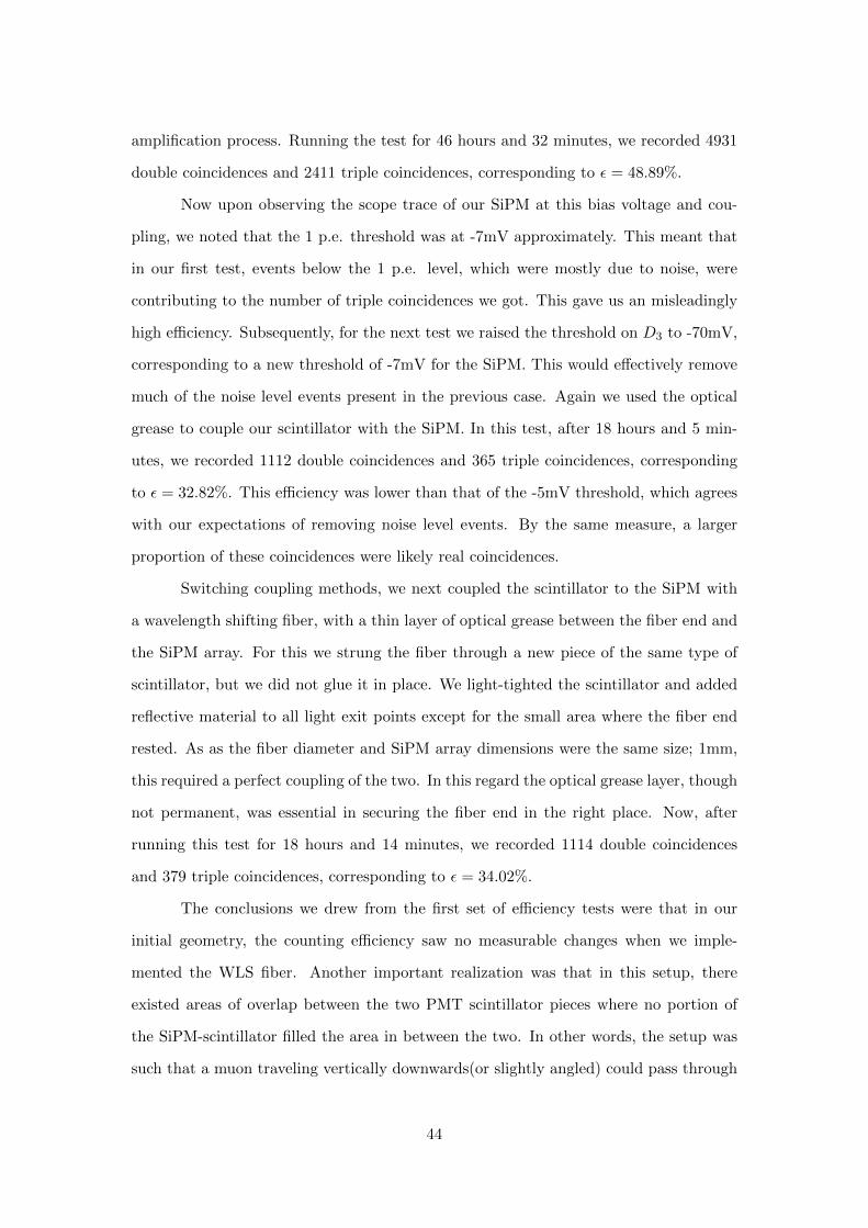
amplification process. Running the test for 46 hours and 32 minutes, we recorded 4931

double coincidences and 2411 triple coincidences, corresponding to ε = 48.89%.

Now upon observing the scope trace of our SiPM at this bias voltage and cou-

pling, we noted that the 1 p.e. threshold was at -7mV approximately. This meant that

in our first test, events below the 1 p.e. level, which were mostly due to noise, were

contributing to the number of triple coincidences we got. This gave us an misleadingly

high efficiency. Subsequently, for the next test we raised the threshold on D3 to -70mV,

corresponding to a new threshold of -7mV for the SiPM. This would effectively remove

much of the noise level events present in the previous case. Again we used the optical

grease to couple our scintillator with the SiPM. In this test, after 18 hours and 5 min-

utes, we recorded 1112 double coincidences and 365 triple coincidences, corresponding

to ε = 32.82%. This efficiency was lower than that of the -5mV threshold, which agrees

with our expectations of removing noise level events. By the same measure, a larger

proportion of these coincidences were likely real coincidences.

Switching coupling methods, we next coupled the scintillator to the SiPM with

a wavelength shifting fiber, with a thin layer of optical grease between the fiber end and

the SiPM array. For this we strung the fiber through a new piece of the same type of

scintillator, but we did not glue it in place. We light-tighted the scintillator and added

reflective material to all light exit points except for the small area where the fiber end

rested. As as the fiber diameter and SiPM array dimensions were the same size; 1mm,

this required a perfect coupling of the two. In this regard the optical grease layer, though

not permanent, was essential in securing the fiber end in the right place. Now, after

running this test for 18 hours and 14 minutes, we recorded 1114 double coincidences

and 379 triple coincidences, corresponding to ε = 34.02%.

The conclusions we drew from the first set of efficiency tests were that in our

initial geometry, the counting efficiency saw no measurable changes when we imple-

mented the WLS fiber. Another important realization was that in this setup, there

existed areas of overlap between the two PMT scintillator pieces where no portion of

the SiPM-scintillator filled the area in between the two. In other words, the setup was

such that a muon traveling vertically downwards(or slightly angled) could pass through

44

the two PMT detector elements without ever hitting the SiPM element. Also, the con-

cern arose that scintillation may actually occur in the light guides, which are nominally

non-scintillating or low scintillating optical conductors between the scintillator and the

PMT. This would increase the negative area of overlap described above. In fact, all of

these factors detracted from the overall efficiency of our SiPM detector, and we sought

to solve these problems in the subsequent experiments.

7.3 Efficiency: Geometry 2

Following the results of our previous experiment, we reoriented the positions of the

two PMTs in relation to the SiPM-scintillator element, seeking to specifically restrict

the vertical overlap of the two PMTs to areas which contained the SiPM-scintillator in

between. To do this we angled the two PMTs, the top PMT with approximately a 45

degree clockwise rotation, and the bottom with an approximately 45 degree counter-

clockwise rotation. This reduced the vertical overlap of the light guides and other parts

of the scintillators. The setup can be seen in figure 35, which we will call geometry 2.

Figure 35: Efficiency Setup: New Geometry

45

For this geometry, we conducted an efficiency test with the SiPM coupled to the

scintillator with the WLS fiber, at an SiPM threshold of -7mV, as before. After 12 hours

and 33 minutes, we recorded 1107 double coincidences and 288 triple coincidences, giving

us ε = 26.01%. Although at first glance we believed we had improved the orientation of

the PMTs, but here we saw our efficiency was actually less than that of geometry 1 in

the WLS case. We are uncertain of the exact cause of this decrease in efficiency, but one

conclusion might be that we actually increased the amount of PMT-scintillator overlap

which we were seeking to decrease.

With a basic structure of our efficiency experiments established, we sought to

investigate the rate of false coincidences in our current setup. The motivation was similar

to that of our false rate studies of section 3.1, with the understanding that because each

discriminator output a pulse of nonzero width, there was inherently a chance that the 3

discriminator pulses would overlap despite the events being out of time, hence creating

a false coincidence. Now for a triple coincidence to occur, the SiPM would have to fire

a discriminator pulse as a double coincidence between the two PMTs was occurring. As

we know the values of the two discriminator output pulse widths for the two PMTs,

we know that the maximum time interval in which a double coincidence can occur

is when the end of one discriminator pulse overlaps with the beginning of the second

discriminator pulse. By that logic, we see that the maximum interval in which this can

occur is simply the sum of the two pulse widths.

Max IntervalDouble Coincidence = PWD1,PMT 1 + PWD2,PMT 2 (6)

Where the PW on the right hand side corresponds to the two discriminator

pulse widths in question. Now if we take into account the rate of the discriminator

output corresponding to the SiPM, we yield a formula for the fractional amount of false

coincidences that will occur.

FCFractional = Max IntervalDouble Coincidence × RateD3,SiPM (7)

Where FCFractional is our fractional amount of false coincidences, and the quan-

46

tities on the right are the variables described above. Now we know the pulse width of

both PMT discriminator pulses to be 46.6ns. Taking into account our SiPM rate given

in table 1, we yield

FCFractional= 0.013

With an expected value for the amount of false coincidences occurring, we sought

to experimentally determine the amount of false coincidences and compare it with our

expected value. To do this, we introduced a time delay to the discriminator output pulse

corresponding to the SiPM, such that when a triple coincidence occurred the third pulse

would be out of time with respect the other two. Hence our counter would not register

a count when an actual triple coincidence occurred. The only way for the counter to

actually register a value would be if the SiPM discriminator pulse occurred before the

discriminator pulses of a double coincidence. As these would be out of time, we see

that this would be a false coincidence. Hence the channel of our counter recording triple

coincidences would actually now correspond to a total count of false triple coincidences,

while the other channel would still correspond to the real count of double coincidences.

The logical elements for this are shown in figure 36, with count A corresponding to the

real count of double coincidences and count B corresponding to the total number of false

triple coincidences.

An example of what occurs when we get a real coincidence in this test setup is

shown in figure 37. In this oscilloscope trace, we see clearly that a real triple coincidence

has occurred. The green square wave corresponds to the delayed discriminator output of

the SiPM. We see that it is delayed approximately 80ns from the time of the coincidence.

We cannot see the discriminator pulses of the PMTs due the the 4-channel maximum of

the oscilloscope, but from previous tests, we know they occur within a few nanoseconds

of the actual coincidence, hence the effective delay of our SiPM discriminator signal is

between 70-80ns. As our PMT discriminator pulses are 46.6ns wide, we see that none

of our real triple coincidences will be recorded by the counter.

After running this test for 18 hours and 38 minutes for the WLS coupling, we

recorded 844 double coincidences and 10 false coincidences, corresponding to a frac-

tional false triple coincidence rate of 0.012. This was very close to our expected value,

47

Figure 36: False Coincidence Test Logical Elements

and helped to validate our procedure for determining the expected value. Ultimately,

geometry 2 yielded a lower efficiency for the WLS coupling than geometry 1. We were

unsure of the exact cause of this, but were still led to believe it may have been cause by

the SiPM-scintillator not covering some of the area where double coincidences occurred.

7.4 Efficiency: Geometry 3

Following our first two detector geometries, we sought to reorient the detector ele-

ment such that there would be no areas where double coincidences could occur without

SiPM-scintillator occupying the space between. The final iteration of our detector ge-

ometry, geometry 3, is shown in figure 38.

Here we see the orientation is close to optimal, and we confirmed with straight

edges that there were no areas of PMT-scintillator overlap which did not contain the

SiPM scintillator in between. Now, with the new setup we proceeded with a few exper-

iments. First, we conducted an efficiency test with the WLS coupling on the SiPM, at

a threshold of -7mV, as before. After 24 hours and 40 minutes, we counted 1563 double

48

Figure 37: False Coincidence Oscilloscope Example

coincidences and 912 triple coincidences, corresponding to an efficiency ε = 58.34%.

This was by far our best efficiency.

Following this, we conducted a false coincidence rate test on the same exact

setup. After 8 hours and 17 minutes, we recorded 544 double coincidences and 13 false

coincidences, giving us a fraction false coincidence rate of 0.024. While this differs from

our expected value of FCFractional= 0.013, the difference is not very large.

For a complete understanding, we then conducted an efficiency and false coin-

cidence rate test for the case of SiPM-scintillator directly coupled with optical grease.

We conducted these tests with the SiPM threshold at -7mV, as with the other cases.

After 11 hours and 55 minutes, we counted 643 double coincidences and 153 triple coinci-

dences, yielding an efficiency of ε = 23.79%. This efficiency was actually lower than that

of geometry 1, which is surprising based on the overlapping area argument described

above as a source of inefficiency.

For the false coincidence rate study, we had to use the rate of the SiPM with

the optical grease coupling to determine our expected fractional false coincidence rate.

49

Figure 38: Efficiency Test Setup: Geometry 3

Taking the appropriate rate from table 1, the same maximum time interval as before,

and solving equation 7, we yield:

FCFractional= 0.014

Now running our false coincidence test for 2 hours and 26 minutes, we yielded

221 double coincidences and 0 false coincidences. This result is low, but does not differ

greatly from our expected rate. Regardless, the efficiency of the optical grease coupling

in geometry 3 was significantly less than that of the WLS coupling.

8 Conclusions

In our study of SiPMs’ performance as the photo-detector element of scintillator

radiation detectors, we learned a number of concrete things. Overall, we have two main

50

cases to consider: our scintillator directly coupled to an SiPM using optical grease, and

our scintillator coupled to an SiPM using a combination of a wavelength shifting fiber

in combination with optical grease. Our initial coincidence rate experiments utilizing 2

SiPMs seemed to show that our counters were inefficient, but in retrospect the use of two

different kinds of SiPM, among other factors, may have greatly hindered the efficiency

of the test setup. In our later counter efficiency tests, we had mixed results, but we

determined with a high degree of certainty that the counter with the WLS coupling in

the third geometry had the greatest efficiency. The efficiency of that case was markedly

higher than that of geometry 1, showing that the improvements in detector orientation

led to a direct increase in our counter’s efficiency. From the large amplitude of the SiPM

signals for triple coincidences, like the example in figure 33, it seems that light collection

is not responsible for the inefficiency. If the light yield of the SiPM-scintillator combina-

tion was small, that would inevitably lead to a lower efficiency. That not being the case,

however, the source of the remaining inefficiency still remains unsolved. Nonetheless, it

shows promise that as we improve the geometrical orientation, the efficiency increases.

Regarding the case of directly coupling the scintillator to the SiPM with optical

grease, we observed that the efficiency was low for all three of our detector orientations.

Though factors such as operating temperature, SiPM array size, and voltage bias may

play a role in the efficiency, it seems that the method of direct coupling is not very

efficient.

Looking forwards, it would be interesting to implement a wavelength shifting film

as a means of coupling the SiPM and scintillator, as that may have a much greater ease of

design and implementation. Also, with a larger dark box and more PMT based counters,

we could greatly improve our efficiency experiments by adding more PMT-scintillator

counters in a more complex geometry. For example using one more PMT and record-

ing the number of triple and quadruple coincidences as opposed to double and triple

coincidences. The study reaffirmed the benefits of using wavelength shifting elements

in photo-detector-scintillator applications, showing that while perhaps not with direct

coupling, SiPMs are viable candidates for large scale detector and HEP experiments.

51

References

[1] Devan, Josh. MINERvA Collaboration

[2] Groupen and Schwartz. Particle Detectors 2nd Edition

[3] Herbert, D.J., D’Ascenzo, N., Belcari, N., Del Guerra, A., Morsani, F., Saveliev, V.

Study of SiPM as a potential photodetector for scintillator readout Nuclear Instru-

ments and Methods in Physics Research A 567 (2006).

[4] M.P. De Pascale et al., J. Geophys. Res. 98, 3501 (1993)

[5] Mai, Carsten. The Tracker of the PERDaix Experiment. February 2010

[6] P.K.F. Grieder,Cosmic Rays at Earth. Elsevier Science (2001)

[7] Pakhlov, P. SiPM: Development and Applications (ITEP). Dec 14,2005.

[8] Para, Adam. Characterization of MPPC/SiPM/GMAPD’s February 17, 2009.

[9] Particle Data Group. Review of Particle Physics.

[10] Pla-Damau, Anna. ”Blue-emitted extruded plastic scintillator with a hole for WLS

fiber.” Notes, September 2012

[11] ”MicroSL Silicon Photomultiplier Detectors Datasheet.” Rev. 1.3, September, 2011.

[12] Tesar, Michal. Scintillator tile and SiPM studies at MPP Munich CALICE elec-

tronics and DAQ and AHCAL main meeting. Hamburg, Germany. December 11,

2012.

52