the dsp workbook - west virginia...

The DSP Workbook

A companion to EE 463

Version 1.0

Spring 2011

Matthew C. Valenti, Ph.D.

West Virginia University

Copyright 2011, Matthew C. Valenti

Preface

This workbook is based on notes used by the author while teaching EE 463, Digital Signal Processing

Fundamentals, at West Virginia University each Spring semester from 2006 to 2010. The book draws

heavily from two textbooks used during those semester:

1. S. K. Mitra, Digital Signal Processing: A Computer-Based Approach, Third Edition, McGraw

Hill, 2006.

2. V. K. Ingle and J. G. Proakis, Digital Signal Processing using Matlab, Second Edition, Thomp-

son, 2007.

In 2011, new editions of both books became available. Many of the exercises and problems in this

work book are modified versions of those found in the above two references. Furthermore, most of

the Matlab functions in this workbook may be found in the Ingle and Proakis book.

The purpose of this workbook is not to duplicate material found in the course texts, but rather

to provide a guide to the in-class lecture. It is expected that both the instructor and student

would bring a hard copy of this workbook to class. During the class, the instructor should cover the

examples and exercises in the workbook, while the student should follow along. The workbook makes

heavy use of Matlab, and the class is best taught in a computer classroom so that each student can

try the exercises on their own using Matlab. You will notice that there are a lot of blank spaces in

the workbook. This is intentional: The student should write the solutions to the exercises in those

spaces.

This book is still a work in progress. There will certainly be several typos or other mistakes.

Catching a mistake is a good sign that you are paying attention! If you find a mistake in this book,

please let me know by emailing me at [email protected].

iii

Contents

1 Discrete-Time Signal Operators 1

1.1 Analog-to-Digital Conversion . . . . . . . . . . . . . . . . . . . . . . . . . . . . . . . 1

1.1.1 Discrete-time Signals . . . . . . . . . . . . . . . . . . . . . . . . . . . . . . . . 2

1.1.2 Representing Signals in Matlab . . . . . . . . . . . . . . . . . . . . . . . . . . 3

1.1.3 The Nyquist Sampling Theorem . . . . . . . . . . . . . . . . . . . . . . . . . 3

1.2 Elementary Sequences . . . . . . . . . . . . . . . . . . . . . . . . . . . . . . . . . . . 4

1.2.1 Unit-Sample Sequence . . . . . . . . . . . . . . . . . . . . . . . . . . . . . . . 4

1.2.2 Unit-Step Sequence . . . . . . . . . . . . . . . . . . . . . . . . . . . . . . . . 4

1.3 Implementing Functions in Matlab . . . . . . . . . . . . . . . . . . . . . . . . . . . . 5

1.4 Unary Signal Operations . . . . . . . . . . . . . . . . . . . . . . . . . . . . . . . . . . 6

1.4.1 Shifting . . . . . . . . . . . . . . . . . . . . . . . . . . . . . . . . . . . . . . . 6

1.4.2 Folding . . . . . . . . . . . . . . . . . . . . . . . . . . . . . . . . . . . . . . . 7

1.4.3 Scalar Multiplication . . . . . . . . . . . . . . . . . . . . . . . . . . . . . . . . 8

1.4.4 Exponentiation . . . . . . . . . . . . . . . . . . . . . . . . . . . . . . . . . . . 8

1.4.5 Sample Summation . . . . . . . . . . . . . . . . . . . . . . . . . . . . . . . . . 9

1.4.6 Signal Energy . . . . . . . . . . . . . . . . . . . . . . . . . . . . . . . . . . . . 9

1.4.7 Signal Power . . . . . . . . . . . . . . . . . . . . . . . . . . . . . . . . . . . . 10

1.4.8 Accumulation . . . . . . . . . . . . . . . . . . . . . . . . . . . . . . . . . . . . 10

1.4.9 Moving Average . . . . . . . . . . . . . . . . . . . . . . . . . . . . . . . . . . 14

1.5 Binary Signal Operations . . . . . . . . . . . . . . . . . . . . . . . . . . . . . . . . . 15

1.5.1 Addition . . . . . . . . . . . . . . . . . . . . . . . . . . . . . . . . . . . . . . . 15

1.5.2 Linear Combination of Signals . . . . . . . . . . . . . . . . . . . . . . . . . . 16

1.5.3 Multiplication . . . . . . . . . . . . . . . . . . . . . . . . . . . . . . . . . . . . 18

1.6 Problems . . . . . . . . . . . . . . . . . . . . . . . . . . . . . . . . . . . . . . . . . . 19

2 Discrete-Time Systems 21

2.1 Discrete-time Systems . . . . . . . . . . . . . . . . . . . . . . . . . . . . . . . . . . . 21

2.2 Exponentially-Weighted Running Average Filter . . . . . . . . . . . . . . . . . . . . 22

2.2.1 Matlab Implementation . . . . . . . . . . . . . . . . . . . . . . . . . . . . . . 22

2.2.2 A Digital-Delay Effect . . . . . . . . . . . . . . . . . . . . . . . . . . . . . . . 23

2.3 System Classifications . . . . . . . . . . . . . . . . . . . . . . . . . . . . . . . . . . . 24

2.3.1 Causality . . . . . . . . . . . . . . . . . . . . . . . . . . . . . . . . . . . . . . 24

2.3.2 Stability . . . . . . . . . . . . . . . . . . . . . . . . . . . . . . . . . . . . . . . 24

v

2.3.3 Linearity . . . . . . . . . . . . . . . . . . . . . . . . . . . . . . . . . . . . . . 25

2.3.4 Time-Invariance . . . . . . . . . . . . . . . . . . . . . . . . . . . . . . . . . . 27

2.4 LTI Systems and Convolution . . . . . . . . . . . . . . . . . . . . . . . . . . . . . . . 29

2.4.1 Convolving in Matlab . . . . . . . . . . . . . . . . . . . . . . . . . . . . . . . 31

2.5 Signal Correlation . . . . . . . . . . . . . . . . . . . . . . . . . . . . . . . . . . . . . 32

2.5.1 Cross-correlation . . . . . . . . . . . . . . . . . . . . . . . . . . . . . . . . . . 33

2.5.2 Determining Time-Delay . . . . . . . . . . . . . . . . . . . . . . . . . . . . . . 33

2.5.3 Relationship with Convolution . . . . . . . . . . . . . . . . . . . . . . . . . . 35

2.5.4 Extended Application Example: Sonar . . . . . . . . . . . . . . . . . . . . . . 36

2.6 Problems . . . . . . . . . . . . . . . . . . . . . . . . . . . . . . . . . . . . . . . . . . 38

3 The Discrete-Time Fourier Transform 41

3.1 Frequency Response . . . . . . . . . . . . . . . . . . . . . . . . . . . . . . . . . . . . 41

3.2 The DTFT . . . . . . . . . . . . . . . . . . . . . . . . . . . . . . . . . . . . . . . . . 43

3.2.1 Properties of the DTFT . . . . . . . . . . . . . . . . . . . . . . . . . . . . . . 44

3.2.2 DTFT of a Finite Sequence . . . . . . . . . . . . . . . . . . . . . . . . . . . . 44

3.2.3 Computing the DTFT in Matlab . . . . . . . . . . . . . . . . . . . . . . . . . 45

3.3 The Inverse DTFT . . . . . . . . . . . . . . . . . . . . . . . . . . . . . . . . . . . . . 47

3.4 Convolving in the Frequency Domain . . . . . . . . . . . . . . . . . . . . . . . . . . . 49

3.5 A Simple Filter Design . . . . . . . . . . . . . . . . . . . . . . . . . . . . . . . . . . . 51

3.6 Difference Equations . . . . . . . . . . . . . . . . . . . . . . . . . . . . . . . . . . . . 52

3.6.1 FIR Systems . . . . . . . . . . . . . . . . . . . . . . . . . . . . . . . . . . . . 52

3.6.2 IIR Systems . . . . . . . . . . . . . . . . . . . . . . . . . . . . . . . . . . . . . 52

3.6.3 The Matlab filter Function . . . . . . . . . . . . . . . . . . . . . . . . . . . . 53

3.6.4 Frequency-Response of a Difference Equation . . . . . . . . . . . . . . . . . . 55

3.6.5 The Matlab freqz and fvtool Functions . . . . . . . . . . . . . . . . . . . . . . 56

3.6.6 Inverting the Frequency Response . . . . . . . . . . . . . . . . . . . . . . . . 57

3.6.7 Approximating an Ideal Lowpass Filter . . . . . . . . . . . . . . . . . . . . . 59

3.6.8 The fdatool . . . . . . . . . . . . . . . . . . . . . . . . . . . . . . . . . . . . . 60

3.7 Problems . . . . . . . . . . . . . . . . . . . . . . . . . . . . . . . . . . . . . . . . . . 61

4 The z-Transfom 65

4.1 Definition of the z-Transform . . . . . . . . . . . . . . . . . . . . . . . . . . . . . . . 65

4.2 Some Important z-Transforms . . . . . . . . . . . . . . . . . . . . . . . . . . . . . . . 66

4.2.1 z-Transform of u[n] . . . . . . . . . . . . . . . . . . . . . . . . . . . . . . . . . 66

4.2.2 z-Transform of −u[−n− 1] . . . . . . . . . . . . . . . . . . . . . . . . . . . . 66

4.2.3 Some Useful z-Transform Pairs . . . . . . . . . . . . . . . . . . . . . . . . . . 66

4.2.4 The z-Transform of Finite Sequences . . . . . . . . . . . . . . . . . . . . . . . 67

4.3 Computing the z-Transform with Matlab . . . . . . . . . . . . . . . . . . . . . . . . 68

4.4 Useful z-transform Properties . . . . . . . . . . . . . . . . . . . . . . . . . . . . . . . 69

4.5 Convolution Using the z-Transform . . . . . . . . . . . . . . . . . . . . . . . . . . . . 69

4.6 System Function . . . . . . . . . . . . . . . . . . . . . . . . . . . . . . . . . . . . . . 70

4.6.1 Poles and Zeros . . . . . . . . . . . . . . . . . . . . . . . . . . . . . . . . . . . 70

4.6.2 ROC and Poles . . . . . . . . . . . . . . . . . . . . . . . . . . . . . . . . . . . 71

vi

4.6.3 Stability . . . . . . . . . . . . . . . . . . . . . . . . . . . . . . . . . . . . . . . 71

4.6.4 Factored Form . . . . . . . . . . . . . . . . . . . . . . . . . . . . . . . . . . . 72

4.6.5 Getting the Difference Equation from Poles and Zeros . . . . . . . . . . . . . 73

4.7 The Inverse z-Transform . . . . . . . . . . . . . . . . . . . . . . . . . . . . . . . . . . 74

4.7.1 Partial-Fraction Expansion . . . . . . . . . . . . . . . . . . . . . . . . . . . . 74

4.7.2 Dealing with Improper Fractions . . . . . . . . . . . . . . . . . . . . . . . . . 76

4.7.3 Inverting the Z-Transform in Matlab . . . . . . . . . . . . . . . . . . . . . . . 77

4.7.4 Repeated Poles . . . . . . . . . . . . . . . . . . . . . . . . . . . . . . . . . . . 78

4.7.5 Complex Poles . . . . . . . . . . . . . . . . . . . . . . . . . . . . . . . . . . . 80

4.8 The poly Function . . . . . . . . . . . . . . . . . . . . . . . . . . . . . . . . . . . . . 81

4.9 Problems . . . . . . . . . . . . . . . . . . . . . . . . . . . . . . . . . . . . . . . . . . 82

5 Digital Filter Structures 85

5.1 The Implementation Problem . . . . . . . . . . . . . . . . . . . . . . . . . . . . . . . 85

5.1.1 Components . . . . . . . . . . . . . . . . . . . . . . . . . . . . . . . . . . . . 85

5.1.2 Goals . . . . . . . . . . . . . . . . . . . . . . . . . . . . . . . . . . . . . . . . 86

5.2 Direct-Form I . . . . . . . . . . . . . . . . . . . . . . . . . . . . . . . . . . . . . . . . 86

5.3 Direct-Form II . . . . . . . . . . . . . . . . . . . . . . . . . . . . . . . . . . . . . . . 87

5.4 Transposed Form . . . . . . . . . . . . . . . . . . . . . . . . . . . . . . . . . . . . . . 88

5.5 Cascade Form . . . . . . . . . . . . . . . . . . . . . . . . . . . . . . . . . . . . . . . . 90

5.5.1 Cascade of First-Order Sections . . . . . . . . . . . . . . . . . . . . . . . . . . 90

5.5.2 Cascade of Second-Order Sections . . . . . . . . . . . . . . . . . . . . . . . . 92

5.6 Parallel Form . . . . . . . . . . . . . . . . . . . . . . . . . . . . . . . . . . . . . . . . 94

5.6.1 First-Order Sections in Parallel . . . . . . . . . . . . . . . . . . . . . . . . . . 94

5.6.2 Second-Order Sections in Parallel . . . . . . . . . . . . . . . . . . . . . . . . . 96

5.7 Problems . . . . . . . . . . . . . . . . . . . . . . . . . . . . . . . . . . . . . . . . . . 98

6 The FFT 99

6.1 Motivation for Finite Transforms . . . . . . . . . . . . . . . . . . . . . . . . . . . . . 99

6.2 Discrete Fourier Series . . . . . . . . . . . . . . . . . . . . . . . . . . . . . . . . . . . 99

6.3 Discrete Fourier Transform . . . . . . . . . . . . . . . . . . . . . . . . . . . . . . . . 100

6.3.1 Relationship with DTFT . . . . . . . . . . . . . . . . . . . . . . . . . . . . . 101

6.3.2 Matlab Implementation . . . . . . . . . . . . . . . . . . . . . . . . . . . . . . 101

6.4 The FFT Algorithm . . . . . . . . . . . . . . . . . . . . . . . . . . . . . . . . . . . . 102

6.5 Circular Convolution . . . . . . . . . . . . . . . . . . . . . . . . . . . . . . . . . . . . 102

6.5.1 Linear Convolution Using the FFT . . . . . . . . . . . . . . . . . . . . . . . . 104

6.5.2 Filtering with the FFT . . . . . . . . . . . . . . . . . . . . . . . . . . . . . . 105

6.6 Problems . . . . . . . . . . . . . . . . . . . . . . . . . . . . . . . . . . . . . . . . . . 106

vii

Chapter 1

Discrete-Time Signal Operators

1.1 Analog-to-Digital Conversion

This course is concerned with the digital processing of signals. If the signal to be processed is ana-

log, then it must first be converted into digital form before processing by using an analog-to-digital

converter (ADC). After digital processing, the signal needs to be brought back into analog form by

using a digital-to-analog converter (DAC). Fortunately, most commercial DSP devices (chips) have

an on-board ADC and DAC. Draw a schematic of a basic DSP system here, making sure

to include the ADC and DAC:

Before continuing, it should be pointed out that an ADC actually performs two operations:

1. Sampling: The analog signal x(t) is a function of the continuous-time variable t which does

not lend itself to a digital representation. The first step in the ADC process is to transform

x(t) into the discrete-time signal x[n]. This process is called sampling. The sampling process

is reversible if the signal is bandlimited and the sample rate is sufficiently high (according to

the Nyquist sampling theorem, which is discussed in the next section).

2. Quantization: Although discrete in time, the samples x[n] are still continuous in amplitude.

To represent digitally, the samples must be quantized by rounding them to one of a finite

set of quantization levels {xq}. If there are Q quantization levels, then each sample may

be represented by a log2(Q) bit quantity. Due to roundoff errors, quantization introduces

distortion that cannot be recovered in the DAC process.

An example of sampling and quantization will be presented in the next section once we establish

some more notation and terminology.

1

2

1.1.1 Discrete-time Signals

Let x(t) be a continuous-time (analog) signal with bandwidth W .1 If x(t) is sampled at a rate of FT

samples per second (or Hz), then the resulting discrete-time signal is:

x[n] = x(nT ) (1.1)

where

T =1

FT(1.2)

is the sample period and n ∈ Z, that is n belongs to the set of all integers {...,−1, 0,+1,+2, ...}.Notice that since there are an infinite number of integer sample instances n, then the number of

samples is infinite (at least in theory). However, in practice, we must restrict ourselves to a finite

number of samples, which implies that n will be a finite set, for instance,

n ∈ {n1, n1 + 1, ..., n2 − 1, n2} (1.3)

where n1 is the first sample instance and n2 is the last sample instance. The length of the sequence

is n2 − n1 + 1. As we will see shortly, when we represent x[n] in Matlab, not only do we need to

indicate the values of the samples x[n] themselves, but we also need to indicate the indices n for

which the samples were evaluated.

Exercise 1.1: Suppose that the signal is x(t) = 72 cos(2πt). The signal is sampled at a rate of

FT = 8 Hz. Determine the set of samples x[n] at sample instances 0 ≤ n ≤ 4. Represent the samples

using a stem diagram.

Exercise 1.2: Now suppose that x[n] is passed through a 3-bit quantizer whose maximum

level matches the maximum value of the signal (so that there is no clipping of the sampled signal).

Determine the value of the samples.

While quantization is an important issue, we will ignore it for most of this workbook and just

consider the behavior of the signal x[n], which is discrete in time but continuous in amplitude.

1The bandwidth of a signal is the range of frequencies for which the energy content is non-negligible.

M.C. Valenti Chapter 1. DT Signal Operators 3

1.1.2 Representing Signals in Matlab

To represent a signal in Matlab, you need to first create the set of sample instances {n1, ..., n2}. This

set can be placed into a row vector n. Next, you need to specify the sample rate FT or equivalently

the sample period T . Finally, the signal can be sampled by evaluating it at x(nT ) for each n in the

vector n. The resulting samples are placed into the vector x, which has the same length as n. Here

is exercise 1.1 done in Matlab:

n = -10:10; % create a vector of sample indices

F_T = 8; % the sample rate

T = 1/F_T; % the sample period

x = cos( 2*pi*n*T ); % the sampled signal

stem( n, x ); % display using a stem diagram

xlabel( ’n’ ); % mark the x-axis

ylabel( ’x[n]’ );% mark the y-axis

1.1.3 The Nyquist Sampling Theorem

The signal x(t) can be unambiguously recovered from x[n] if FT ≥ 2W . Otherwise aliasing will

occur.

Exercise 1.3: Sample the signal cos(2πt) at a rate of FT = 3/2 Hz. Use Matlab.

Exercise 1.4: Now sample the signal cos(πt) at a rate of FT = 2/3 Hz. Again, use Matlab.

4

1.2 Elementary Sequences

The following sequences will be used throughout the workbook, and are useful for illustrating key

concepts.

1.2.1 Unit-Sample Sequence

The unit-sample sequence δ[n] is defined as:

δ[n] =

1 for n = 0

0 for n 6= 0(1.4)

where n runs from n1 to n2. This signal can be created in Matlab as follows (in this example,

n1 = −10 and n2 = +10)


x = (n==0); % creates a ’1’ where n=0, and a ’0’ elsewhere




This signal is also called an impulse sequence.

1.2.2 Unit-Step Sequence

The unit-step sequence u[n] is defined as:

u[n] =

1 for n ≥ 0

0 for n < 0(1.5)

where n again runs from n1 to n2. This signal can be created in Matlab as follows (in this example,

n1 = −10 and n2 = +10)


x = (n>=0); % creates a ’1’ where n>=0, and a ’0’ elsewhere





1.3 Implementing Functions in Matlab

Throughout this course, you will be asked to create your own Matlab functions. A function is an

entity that takes in one or more inputs and produces one or more outputs. To start, let’s create a

function for generating an impulse (type “edit” in Matlab to bring up the editor). The function

needs to be stored as its own file (with a “.m” extension). Create a file called “impseq.m” with the

following contents:

function [x,n] = impseq( n1, n2)

% Generates x[n] = delta[n]

% and the indices n = [n1, ..., n2]

% note that n2 > n1 for this to work

n = [n1:n2];

x = (n==0);

Notice that the function takes in two inputs: n1 and n2, and that it creates two outputs, the vector x

containing the sample values and the vector n containing the sample instances. Back in the Matlab

command space, the function may be called as follows:

n1 = -10; % first sample instant

n2 = +10; % last sample instant

[x,n] = impseq( n1, n2 ); % the impulse sequence




Exercise 1.5: Create a function that generates a unit-step sequence. Call the function “stepseq”.

6

1.4 Unary Signal Operations

Unary operations are operations that work on just one signal. Later, we will discuss binary operations

which act on two signals (not to be confused with binary number systems!), but for now, let’s go

over some basic unary signal operations.

1.4.1 Shifting

One of the most basic operations in a DSP system is to shift the time reference. The shift may be

considered either a delay or an advance. Delays are more common than advances, especially if the

processing must be done in real-time and must be causal. A signal y[n] may be defined to be x[n]

delayed by n0 samples as follows:

y[n] = x[n− n0] (1.6)

If n0 > 0, the signal has been delayed, while if n0 < 0 the signal has been advanced.

Exercise 1.6: Prove the following expression for a time-shifted unit-sample sequence:

δ[n− n0] =

1 for n = n0

0 for n 6= n0.(1.7)

We can use this to modify our “impseq” program so that it now takes three arguments, with n0

being a new argument:

function [x,n] = impseq( n0, n1, n2)

% Generates x[n] = delta[n-n0]

% and the indices n = [n1, ..., n2]

% note that n2 > n1 for this to work

n = [n1:n2];

x = (n==n0);

Similarly, it can be shown that:

u[n− n0] =

1 for n ≥ n00 for n < n0.

(1.8)

and a similar change may be done to the “stepseq” function.


More generally, the signal x[n − n0] is identical to the signal x[n] except that the sample that

was at n = 0 is now shifted to be at n = n0. The following Matlab function will delay any sequence

by n0 samples:

function [y,n] = sigshift(x,n,n0)

% Generates y[n] = x[n-n0]

n = n + n_0; % new time axis

y = x; % the sample sequence remains untouched

Exercise 1.7: Let x[n] = cos(πn/8) for −16 ≤ n ≤ 16. On the same stem diagram, plot x[n] and

x[n− 4]. You should use the sigshift function to complete this exercise.

1.4.2 Folding

Folding involves the reversal of the time axis. So instead of the signal indices running from n1 to

n2, they now run from −n2 to −n1. This is written as:

y[n] = x[−n] (1.9)

In Matlab, this can be implemented with the help of Matlab’s “fliplr” function. The following

function performs a folding operation:

function [y,n] = sigfold(x,n)

% implements y(n) = x(-n)

% -----------------------

% [y,n] = sigfold(x,n)

%

n = -fliplr(n); % reverse the time axis

y = fliplr(x); % sample values are unchanged

8

Exercise 1.8: Let x[n] = exp(n/5) for −5 ≤ n ≤ 15. Plot x[n] and y[n] = x[−n] on the same stem

diagram.

1.4.3 Scalar Multiplication

We can multiply a signal by a scalar value such as ‘c’, which is represented by:

y[n] = cx[n] (1.10)

In Matlab, multiplication is performed with the asterisk key ‘∗’, i.e.

y = c*x;

Multiplication does not change the time axis. Note that later in the notes, we will use ‘∗’ to denote

convolution, so you need to be mindful of this distinction.

Exercise 1.9: For the signal x[n] defined in Exercise 1.8, plot y[n] = 4x[n]. Use Matlab.

1.4.4 Exponentiation

In some cases, we might want to square each sample in a sequence, resulting in a new sequence. The

notation

y[n] = (x[n])2 (1.11)

is interpreted as follows: The nth sample of the signal y[n] is found by squaring the sample x[n]. More

generally, we can raise a signal to the `th power, i.e. y[n] = (x[n])`. In Matlab, signal exponentiation

is performed using

y = x.^2;

Exercise 1.10: Using Matlab, plot y[n] = (x[n])2, where x[n] = cos(πn/8) and −16 ≤ n ≤ 16.


1.4.5 Sample Summation

Another basic operation is to add up a sequence of consecutive samples. For instance, we could add

samples with time indices ranging from n1 to n2 as follows:

c =

n2∑n=n1

x[n] = x[n1] + x[n1 + 1] + ...+ x[n2]. (1.12)

Note that the result of this type of sample summation is a scalar value, not a signal (i.e. the time

index is lost since we’ve summed over it). Summation is performed in Matlab using the “sum”

function. For instance,

c = sum(x)

will give the sum of all the samples stored in the vector x.

Exercise 1.11: Use Matlab to find the sum of all samples of the y[n] found in Exercise 1.10.

Now find the sum of all samples with nonnegative index (i.e. all y[n] for which n ≥ 0).

1.4.6 Signal Energy

The energy of a signal x[n] that is defined over indices ranging from n1 to n2 is found by performing

a sample summation of the signal |x[n]|2 i.e.

Ex =

n2∑n=n1

|x[n]|2. (1.13)

Exercise 1.12: Use Matlab to find the energy of x[n] = cos(πn/8) and −16 ≤ n ≤ 16.

10

1.4.7 Signal Power

The power of a signal x[n] that is defined over indices ranging from n1 to n2 is found by dividing

the energy by the number of samples n2 − n1 + 1, i.e.

Px =Ex

n2 − n1 + 1. (1.14)

If the signal duration is infinite, then this becomes a limiting operation,

Px = limK→∞

1

2K + 1

K∑n=−K

|x[n]|2. (1.15)

If the signal is periodic with period N then

Px = limK→∞

1

N

N−1∑n=0

|x[n]|2 (1.16)

where the summation may be over any one period.

Exercise 1.13: Use Matlab to find the power of x[n] = cos(πn/8).

1.4.8 Accumulation

We can use the idea of sample summation to create a signal if we allow the limits to depend on n.

An accumulator performs sample summation with n1 = −∞ and n2 = n. This relationship can be

expressed as:

y[n] =

n∑`=−∞

x[`]. (1.17)

The result is now a signal y[n] because the upper limit in the summation depends on n. Notice that

since n is now in the limits of the summation, we need to use a different index of summation (in

this case, `).

Now perform a change of variables, letting ` = n− k. This gives an alternative expression:

y[n] =

∞∑k=0

x[n− k]. (1.18)

The interpretation of this equation is that y[n] is equal to the sum of the current sample x[n] and

all past samples.


Recursive Representation of Accumulation

Notice that the two equations (1.17) and (1.18) are equivalent. Thus, it is apparent that a given

signal operation can be represented in more than one way. Are there any other ways to represent

the accumulation operation? It turns out that another way is:

y[n] = x[n] + y[n− 1] (1.19)

Proof: Rewrite (1.18) using m as the index of summation:

y[n] =

∞∑m=0

x[n−m]. (1.20)

Now delay both sides by one sample period:

y[n− 1] =

∞∑m=0

x[(n− 1)−m]

=

∞∑m=0

x[n− (m+ 1)] (1.21)

Now change the index of summation to k = m+ 1,

y[n− 1] =

∞∑k=1

x[n− k]. (1.22)

Finally, subtract (1.22) from (1.18),

y[n]− y[n− 1] =

∞∑k=0

x[n− k]−∞∑k=1

x[n− k]

= x[n] (1.23)

where the second line follows from the fact that the only difference between the two summations is

that the first summation has k = 0 term but the second one does not. Now, solve (1.23) for y[n] to

get:

y[n] = x[n] + y[n− 1] (1.24)

This expression is said to be recursive because each output depends on past outputs. An accumulator

is one of the simplest types of Infinite Impulse Response (IIR) filters.

12

Pictorial Representation of Accumulation

Most signal operations of interest can be represented with the help of block diagrams. Alternatively,

signal-flow diagram may be used. The basic elements for these diagrams are pictured below:

Component Block Diagram Signal-flow Diagram

Multiplier

Delay

Adder

z-1

c

z-1

+

To implement an accumulator, we only need two types of elements: An adder and a unit delay. The

multiplier will prove useful for other systems.

Exercise 1.14: Draw block-diagram and signal-flow diagram representations of equation (1.24).


Implementing an Accumulator in Matlab

Now, let’s develop an accumulator in Matlab. We will basically be implementing equation (1.24) as

a function. One issue we need to deal with is that, because of the recursive nature of the system,

the length of the output could be infinite even if the length of the input is finite. Because of this,

the system is said to have an infinite impulse response and is classified as an IIR system. To handle

this problem, we will limit the length of the output to be the same as the input. If we want to make

the output longer, we can extend the length of the input by padding it with zeros (i.e. just append

a sequence of zeros at the end of the sequence).

Here is a function that will perform accumulation:

function [y,m] = accumulate(x,n)

% implements y(n) = x(n) + y(n-1)

% -------------------------

% [y,m] = accumulate(x,n)

%

m = n; % no change in time axis

y = zeros( size(x) ); % need to preallocate y

y(1) = x(1); % first output sample

for index=2:length(n)

y(index) = x(index) + y(index-1);

end

Exercise 1.15: Let x[n] = δ[n] over −5 ≤ n ≤ 15. Using the “accumulate” function, plot y[n] =

x[n]+y[n−1] over the same range of n. What is the relationship among δ[n], u[n], and accumulation?

Repeat this exercise for x[n] = u[n] and comment about the stability of the accumulation function.

14

1.4.9 Moving Average

Another way to create a signal using the idea of sample summation is to take the average of M

samples (the current sample and past M − 1 samples). This is an M-point average, and may be

written as:

y[n] =1

M

M−1∑k=0

x[n− k] (1.25)

This is also called a moving average and is one of the simplest types of Finite Impulse Response

(FIR) filters. Notice that the time averaging operation given in (1.25) is similar to the accumulator

as given in (1.18) except that the expressions are different in two ways: What are they?

Pictorial Representation of a Moving Average

Besides adding and delaying signals, we also need the ability to perform a scalar multiplication

operation, which can be represented pictorially with a multiplier.

Exercise 1.16: Draw block-diagram and signal-flow diagram representations of equation (1.25)

for the case that M = 4.


1.5 Binary Signal Operations

We would also like to perform operations on two signals, such as addition and multiplication of

signals. Such operations are called binary because they have two arguments. This section describes

some basic binary operations. A more complicated binary signal operation is discrete-time convolu-

tion which is described in the next chapter.

1.5.1 Addition

Addition of two signals implies that samples at the same time instant are added together. As an

example:

y[n] = x1[n] + x2[n] (1.26)

Adding two signals defined over the same time scale is easy in Matlab. For instance:

n = 0:12;

x1 = exp(-n/4);

x2= cos(pi*n/4);

y = x1 + x2;

However, things get more complicated when the two signals don’t have the same time scale. A new

time axis needs to be created that is the union of the two time axes. For instance, if signal x1[n] is

defined for −4 ≤ n ≤ 8 and x2[n] is defined for 0 ≤ n ≤ 12, then the sum y[n] = x1[n] + x2[n] must

be defined over −4 ≤ n ≤ 12.

Adding Signals in Matlab

The following program can be used to add two signals with different time axes:

function [y,n] = sigadd(x1,n1,x2,n2)

% implements y(n) = x1(n)+x2(n)

% -----------------------------

% [y,n] = sigadd(x1,n1,x2,n2)

% y = sum sequence over n, which includes n1 and n2

% x1 = first sequence over n1

% x2 = second sequence over n2 (n2 can be different from n1)

%

n = min(min(n1),min(n2)):max(max(n1),max(n2)); % duration of y(n)

y1 = zeros(1,length(n));

y2 = y1; % initialization

y1(find((n>=min(n1))&(n<=max(n1))==1))=x1; % x1 with duration of y


y = y1+y2; % sequence addition

16

Exercise 1.17: Using “sigadd”, add x1[n] = exp(−n/4),−4 ≤ n ≤ 8 with x2[n] = cos(πn/4), 0 ≤n ≤ 12. Plot x1[n], x2[n], and y[n].

1.5.2 Linear Combination of Signals

Suppose we have M signals x0[n], x1[n], ..., xM−1[n]. We could add them all together to form a new

signal:

y[n] =

M−1∑k=0

xk[n]. (1.27)

More generally, we could multiply each signal xk[n] by a scalar value ck to obtain a signal

y[n] =

M−1∑k=0

ckxk[n]. (1.28)

Such a signal is said to be a linear combination of the signals x0[n], x1[n], ..., xM−1[n].

Exercise 1.18: A moving average is a linear combination of the signals x[n], x[n−1], ..., x[n− (M−1)]. What are the values of the coefficients ck?


Unit-Sample Synthesis

Any signal x[n] can be represented as a linear combination of delayed unit-sample sequences:

x[n] =

n2∑k=n1

x[k]δ[n− k]. (1.29)

Exercise 1.19: Represent the following sequence as a linear combination of delayed unit-sample

sequences

x[n] =

{2,−4

↑, 1,−2

}. (1.30)

Unit-Step Synthesis

Similarly, it is possible to represent x[n] as a linear combination of unit-step sequences.

Exercise 1.20: Represent the previous x[n] as a linear combination of delayed unit-step sequences.

18

1.5.3 Multiplication

Multiplication of two signals is analogous to addition, i.e. samples at the same time instant are

added together. This is written as:

y[n] = x1[n] · x2[n] (1.31)

To multiply signals in Matlab with the same time scale, use ‘.*’

n = 0:12;

x1 = exp(-n/4);

x2= cos(pi*n/4);

y = x1.*x2;

The period before the asterisk is important because it signals Matlab to perform an element-by-

element operation. Without the period, it will try to do a vector-vector multiply (which will fail due

to mismatched dimensions).

To multiply signals with different axes, you may use:

function [y,n] = sigmult(x1,n1,x2,n2)

% implements y(n) = x1(n)*x2(n)

% -----------------------------

% [y,n] = sigmult(x1,n1,x2,n2)

% y = product sequence over n, which includes n1 and n2

% x1 = first sequence over n1

% x2 = second sequence over n2 (n2 can be different from n1)

%

n = min(min(n1),min(n2)):max(max(n1),max(n2)); % duration of y(n)

y1 = zeros(1,length(n)); y2 = y1; %



y = y1.* y2;

Exercise 1.21: Using “sigmult”, multiply x1[n] = exp(−n/4),−4 ≤ n ≤ 8 with x2[n] = cos(πn/4), 0 ≤n ≤ 12.


1.6 Problems

1. Consider the following sequences:

x[n] = {−4, 5, 1,−2,−3, 0, 2} ,−3 ≤ n ≤ 3

y[n] = {6,−3,−1, 0, 8, 7,−2} ,−1 ≤ n ≤ 5

w[n] = {3, 2, 2,−1, 0,−2, 5} , 2 ≤ n ≤ 8.

The sample values of each of the above sequences outside the ranges specified are all zeros.

Generate the following sequences:

(a) c[n] = x[−n+ 2].

(b) d[n] = y[−n− 3].

(c) e[n] = w[−n].

(d) f [n] = x[n] + y[n− 2].

(e) v[n] = x[n] · w[n+ 4].

(f) s[n] = y[n]− w[n+ 4].

(g) r[n] = 3.5y[n].

You may either do these by hand (i.e. with paper-and-pencil) or by using Matlab (in which

case, you should turn in your plots and the commands used to generate them).

2. (a) Express the sequences x[n], y[n] and w[n] of Problem 1 as a linear combination of delayed

unit sample sequences.

(b) Express the sequences x[n], y[n] and w[n] of Problem 1 as a linear combination of delayed

unit step sequences.

3. Compute the energy of each of the sequences x[n], y[n] and w[n] of Problem 1.

4. Plot each of the following sequences (using a stem diagram):

x1[n] = 3δ[n+ 2] + 2δ[n]− δ[n− 3] + 5δ[n− 7].

x2[n] =

5∑k=−5

e|k|δ[n− 2k].

x3[n] = 10u[n]− 5u[n− 5]− 10u[n− 10] + 5u[n− 15].

x4[n] = e0.1n (u[n+ 20]− u[n− 10]) .

The sample values of each of the above sequences outside the ranges specified are all zeros.

Again, you may either do these by hand (i.e. with paper-and-pencil) or by using Matlab (in

which case, you should turn in your plots and the commands used to generate them).

Chapter 2

Discrete-Time Systems

2.1 Discrete-time Systems

A discrete-time system is an entity that processes one or more discrete-time input sequence(s) to

produce a discrete-time output sequence. We have already seen many examples of single-input

discrete-time systems:

1. Time Shifter: y[n] = x[n− n0], for a fixed delay n0.

2. Signal Folder: y[n] = x[−n].

3. Scalar Multiplier: y[n] = cx[n], for a fixed multiplier c.

4. Exponentiation: y[n] = (x[n])k, for a fixed exponent k.

5. Accumulator: y[n] = x[n] + y[n− 1].

6. FIR filter: y[n] =∑Mk=0 bkx[n− k], for a fixed set of coefficients {bk}.

7. Moving-average: y[n] =∑M−1k=0

1M x[n− k], for a fixed value of M .

Discrete-time systems may also have two (or more) inputs. Examples of systems that have two

inputs include:

1. Adder: y[n] = x1[n] + x2[n].

2. Mixer (a.k.a. Multiplier): y[n] = x1[n] · x2[n].

Although multiple-input systems certainly have some important applications (such as signal cross-

correlation), let’s begin by discussing single-input systems in detail. Before delving into systems in

general, let’s look at one more specific system ...

21

22

2.2 Exponentially-Weighted Running Average Filter

Recall that the main problem with the accumulator is that it is unstable. This is evident because

the step-response is a ramp function, and thus as n→∞, then y[n]→∞, i.e. the output tends to

an infinite value, which will eventually exceed the maximum value that can be represented on the

digital system. We can stabilize the filter by dampening the signal which is fed back to the input as

follows:

y[n] = x[n] + αy[n− 1] (2.32)

where |α| < 1 is required to assure stability. An exponentially-weighted running average filter is a

system that implements this equation.

2.2.1 Matlab Implementation

Exercise 2.1: Create a function called expavg which implements an exponentially-weighted running

average filter. Use the accumulate function as a starting point. You will need an additional input,

which is the value of α. The function should begin like this:

function [y,m] = expavg(x,n,alpha)

% implements y(n) = x(n) + alpha*y(n-1)

% -------------------------

% [y,m] = expavg(x,n,alpha)

%

Using your function, determine the impulse and step responses for α = 0.85 over −5 ≤ n ≤ 25.

M.C. Valenti Chapter 2. DT Systems 23

2.2.2 A Digital-Delay Effect

Digital Delay is a common effect used to process audio signals. A digital delay is merely an

exponentially-weighted running average filter with a delay that may be more than just one sam-

ple. We can write this as:

y[n] = x[n] + αy[n− n0], (2.33)

where the value of n0 depends on the desired time delay. If the signal was sampled at a rate of FT

samples per second, then the delay in seconds Td will be:

Td =n0FT

. (2.34)

Exercise 2.2: Create a function called digitaldelay which implements a digital delay effect. Use the

expavg function as a starting point. You will need an additional input, which is the value of n0. The

function should look like this:

function [y,m] = digitaldelay(x,n,alpha,n0)

% implements y(n) = x(n) + alpha*y(n-n0)

% -------------------------

% [y,m] = digitaldelay(x,n,alpha,n0)

%

m = n; % no change in time axis

y = zeros(size(n)); % preallocate the output

y(1:n0) = x(1:n0); % first n0 output samples

start = n0+1; % start loop *after* the n0’th sample

for index=start:length(n)

y(index) = x(index) + alpha*y(index-n0);

end

Let’s use this function to process an actual audio signal stored in a .wav file (there is one on the

eCampus page called dave.wav for you to use 1). You will need to use the wavread function to read

the wav file into Matlab and the sound function to play it through your speakers. I suggest that you

append some zeros to the end of the sequence before running it through the digital delay (otherwise

the output will get truncated to the length of the input, and you won’t hear the trailing echoes).

[z,fs] = wavread( ’dave’ ); % read the file

sound( z, fs ); % listen to the original signal

x = z’; % make the samples a row vector.

x = [x zeros(1,2*fs)]; % add two seconds of silence

n = 0:( length(x) - 1 ); % the discrete-time axis

alpha = 0.5; % dampening factor

Td = 0.5; % half-second delay

n0 = round(fs*Td); % integer number of samples in a half second

[y,m] = digitaldelay(x,n,alpha,n0); % pass through the digital delay

sound( y, fs ); % listen to the processed signal

You could repeat this for other .wav files that you can find on the Internet, and you could experiment

with different delays Td and dampening coefficients α. You can record your own audio by using the

wavrecord function (Windows only) or by creating an audiorecorder object.

1Trivial: What movie is the clip from?

24

2.3 System Classifications

Systems can be classified in several different ways. They can be linear or nonlinear; they can be time-

invariant or time-varying; they can be stable or unstable; they can be causal or anti-causal. Below,

we will describe these four binary alternatives. In doing so, we will use the following notation:

y[n] = T (x[n]) (2.35)

To represent the I/O relationship of a system.

2.3.1 Causality

A system is causal if the output y[n0] at time n0 does not depend on future inputs x[n], n > n0.

A system that is not causal is said to be anit-causal or anticipatory. While strictly speaking, all

physically-realizable systems must be causal, a system may exhibit anti-causal behavior if it processes

recorded or delayed data (since when working with a recording, the processor has access to samples

that are relatively earlier in time).

• Exercise 2.3: A particular FIR system is described by the I/O relationship

y[n] =

m2∑k=m1

bkx[n− k] (2.36)

for some integers m1 and m2, where m2 > m1. Is this FIR system necessarily causal? What

must be true about m1 to assure causality?

• Exercise 2.4: Is the signal folding operation causal?

2.3.2 Stability

A system is stable if for every bounded input x[n], i.e. an input which satisfies,

|x[n]| < Bx, for all n

the corresponding output is bounded, i.e. it satisfies,

|y[n]| < By, for all n.

In the above two equations Bx and By represent finite constants.


• Exercise 2.5: Is the exponentially-weighted running average filter (y[n] = x[n] + αy[n − 1])

causal? What must be true of α to assure stability?

• Exercise 2.6: Is the FIR system (y[n] =∑Mk=0 bkx[n− k]) stable? You may assume all coef-

ficients bk are finite and that M is finite.

2.3.3 Linearity

Suppose we have a discrete-time system with I/O relationship y[n] = T (x[n]). It follows that:

y1[n] = T (x1[n])

y2[n] = T (x2[n]) ,

i.e., the output is y1[n] when the input is x1[n], and the output is y2[n] when the input is x2[n].

Now create an input xc[n] which is a linear combination of x1[n] and x2[n],

x[n] = αx1[n] + βx2[n]

where α and β are arbitrary coefficients. Then the system is said to be linear if

T (x[n]) = T (αx1[n] + βx2[n])

= αT (x1[n]) + βT (x2[n])

= αy1[n] + βy2[n]

= αT (x1[n]) + βT (x2[n]) (2.37)

A system that is not linear is said to be non-linear.

• Exercise 2.7: Is exponentiation y[n] = (x[n])k linear for k 6= 1?

26

• Exercise 2.8: Is the FIR system y[n] =∑Mk=0 bkx[n− k] linear?

• Exercise 2.9: Is the system y[n] = x[n] + c linear for c 6= 0?

• Exercise 2.10: Is the accumulator y[n] = x[n] + y[n− 1] linear?


Importance of Linearity

Recall that any signal may be expressed as a linear combination of delayed impulses (c.f. unit-sample

synthesis),

x[n] =

∞∑k=−∞

x[k]δ[n− k]. (2.38)

Let the above x[n] be an input to a linear system. The output is

y[n] = T (x[n])

= T

( ∞∑k=−∞

x[k]δ[n− k]

)

=

∞∑k=−∞

x[k]T (δ[n− k])︸︷︷︸h[n,k]

=

∞∑k=−∞

x[k]h[n, k] (2.39)

where h[n, k] the response of the system to an impulse applied at time k.

2.3.4 Time-Invariance

A system is time-invariant or shift-invariant if a shift in the input signal produces a corresponding

shift in the output. More precisely, if

T (x[n]) = y[n] (2.40)

then

T (x[n− 1]) = y[n− 1]. (2.41)

• Exercise 2.11: Is the system y[n] = nx[n] time-invariant?

28

• Exercise 2.12: Is the folding operation time-invariant?

• Exercise 2.13: Is the FIR system (y[n] =∑Mk=0 bkx[n− k]) time-invariant?


2.4 LTI Systems and Convolution

We already saw that if the system is linear, then the output can be expressed as:

y[n] =

∞∑k=−∞

x[k]h[n, k] (2.42)

where h[n, k] is the response of an impulse applied at time k. Suppose an impulse is applied at time

k = 0, i.e. the input is x0[n] = δ[0], then the output is:

y0[n] = h[n, 0]. (2.43)

Now, suppose that the impulse is delayed by one sample period so that the input is x1[n] = x0[n−1] =

δ[1]. The output is

y1[n] = h[n, 1]. (2.44)

However, since it is also time-invariant, then it follows that y1[n] = y0[n− 1], and thus

y1[n] = h[n− 1, 0]. (2.45)

By equating equations (2.44) and (2.45), we see that

h[n, 1] = h[n− 1, 0]. (2.46)

It follows that

h[n, k] = h[n− k, 0]. (2.47)

That is, the response to an impulse applied at time k is simply a shifted version of the response to

an impulse applied at time 0. Substituting (2.47) into (2.42), we get:

y[n] =

∞∑k=−∞

x[k]h[n− k, 0]. (2.48)

Since we are now only concerned with the response to an impulse applied at time 0, we may drop

the second argument of the function h and simply write it as h[n− k]

y[n] =

∞∑k=−∞

x[k]h[n− k]. (2.49)

The function h[n] is called the impulse response of the system and the above operation is called

convolution,

y[n] = x[n] ∗ h[n] =

∞∑k=−∞

x[k]h[n− k]. (2.50)

30

Exercise 2.14: Convolve the following two sequences:

x[n] = {5↑, 1, 3}

h[n] = {6↑, 4, 2}


Keeping Track of Time

A common mistake when convolving two sequences is to lose track of the time reference. The

following rule should (hopefully) help you to avoid such a mistake:

• Suppose that x[n] is nonzero over the range N1,x ≤ n ≤ N2,x and h[n] is nonzero over the

range N1,h ≤ n ≤ N2,h.

• Then y[n] = x[n] ∗ h[n] will be nonzero over the range (N1,x +N1,h) ≤ n ≤ (N2,x +N2,h).

• Alternatively, you could say that y[n] is nonzero over the range N1,y ≤ n ≤ N2,y where

N1,y = N1,x +N1,h and N2,y = N2,x +N2,h.

The last interpretation provides guidance on how to implement convolution in Matlab.

2.4.1 Convolving in Matlab

The Matlab conv function will give the result of convolving two sequences. However, conv does not

keep track of the time reference. In order to keep track of time, the following function, called conv m

should be used:

function [y,ny] = conv_m(x,nx,h,nh)

% Modified convolution routine for signal processing

% --------------------------------------------------

% [y,ny] = conv_m(x,nx,h,nh)

% y = convolution result

% ny = support of y

% x = first signal on support nx

% nx = support of x

% h = second signal on support nh

% nh = support of h

%

nyb = nx(1)+nh(1); nye = nx(length(x)) + nh(length(h));

ny = [nyb:nye];

y = conv(x,h);

Exercise 2.15: Repeat Exercise 2.14 using Matlab.

32

Causal LTI Systems

An LTI system with impulse response h[n] is causal if and only if h[n] = 0 for all n < 0.

Stable LTI Systems

An LTI system with impulse response h[n] is stable if and only if its impulse response is absolutely

summable:

∞∑n=−∞

|h[n]| < ∞ (2.51)

Exercise 2.16: Is the exponentially-weighted running average: y[n] = x[n] + αy[n− 1] stable?

2.5 Signal Correlation

There are many engineering applications where you need to compare the similarity of two signals:

1. Ranging: A reference radar or sonar signal is transmitted and reflected off a target. The

received signal should be similar to the transmitted signal, except that it will contain random

noise and will be delayed by a time that depends on the distance. The goal of the receiver is

to estimate the delay, which will allow the range to be determined.

2. Digital Communications: Depending on the value of a data bit, one of two waveforms

are transmitted over a noisy channel. The receiver needs to decide which waveform was

transmitted by comparing the received signal against the two possible waveforms. Once the

receiver determines which waveform was transmitted, it can determine the value of the data

bit.


2.5.1 Cross-correlation

Correlation is a test of similarity between two signals. In its simplest form, the correlation of two

signals x[n] and w[n] is merely

rxw =

∞∑k=−∞

x[n]w[n] (2.52)

which is the sample sum of the product of the two signals. Suppose that x[n] and w[n] have the

same energy E and that they may or may not be the same signal. If the two signals are the same

(x[n] = w[n]), then rxw will take on a large value, namely the energy of the signal, i.e. rxw = E .

On the other hand, if the two signals are not the same (x[n] 6= w[n]) then rxw will have a smaller

magnitude, i.e. |rxw| ≤ E .

Although simple, (2.52) suffers from an inability to tell if w[n] is just a time-shifted version

of x[n]. To handle time-shifts, we need a more generalized version of (2.52), which is called the

cross-correlation sequence:

rxw[`] =

∞∑n=−∞

x[n]w[n− `] (2.53)

where the parameter ` is called the lag and is an integer value.

2.5.2 Determining Time-Delay

Suppose that x[n] = w[n − n0], where n0 is an unknown time offset. Then the value of the cross-

correlation function will be at its maximum value at lag ` = n0

rxw[n0] =

∞∑n=−∞

w[n− n0]︸︷︷︸x[n]

w[n− n0] =

∞∑k=−∞

w[k]w[k] = E (2.54)

where the change of variables k = n− n0 was used in going from the first summation to the second

one. At all other values of lag, |rxw| ≤ E . Thus, to identify the the value of the delay n0, all you

need to do is compute the cross-correlation between x[n] and w[n] and then pick the value of ` for

which the cross-correlation is at its peak,

n0 = arg max rxw[`] (2.55)

where the “arg max” operator returns the index of the maximum value in the sequence rxw[`].

34

Exercise 2.17: Let w[n] and x[n] be:

w[n] = {2↑, 1, 4}

x[n] = {0↑, 0, 2, 1, 4}.

As you can see, x[n] is a delayed version of w[n]. Compute the cross-correlation sequence for

0 ≤ ` ≤ 4. Use the cross-correlation sequence to estimate the value of the time delay n0.


2.5.3 Relationship with Convolution

We may also compute the cross-correlation sequence as:

rxw[n] = x[n] ∗ h[n] (2.56)

where ∗ is the convolution operation

x[n] ∗ h[n] =

∞∑k=−∞

x[k]h[n− k] (2.57)

and h[n] is

h[n] = w[−n]. (2.58)

The discrete-time system implementing this convolution is called a matched filter.

Proof:

Exercise 2.18: Redo Exercise 2.17 in Matlab using a matched filter.

36

2.5.4 Extended Application Example: Sonar

In a sonar system, a time-domain waveform is transmitted:

w(t) = cos(ωct), for 0 ≤ t ≤W (2.59)

where ωc = 2πfc and fc is the transmitted tone (in Hz). A typical value might be fc = 500 Hz. The

signal travels at the speed of sound, is reflected by a surface and is received as

x(t) = w(t− td) + η(t) (2.60)

where v(t) is noise. The time delay td is related to the distance to the object and the speed of sound

v by:

2d = vtd. (2.61)

The speed of sound through room-temperature air is 331.3 m/sec. The factor of 2 in the above

equation accounts for the fact that td is the round-trip delay. Solving for d, we find that the distance

is:

d =vtd2. (2.62)

Since this is a DSP class, we will implement the receiver digitally. Let’s sample x(t) at a rate of

fs = 10 kHz. The sampled signal becomes:

x[n] = x(nT ) = w[n− nd] + η[n] (2.63)

where η[n] is sampled noise and nd is the time delay in units of samples (instead of units of seconds),

found as:

nd = round(tdfs) (2.64)

where the rounding is necessary to make nd an integer.

The goal of the receiver is to estimate nd, which it can then use to determine the distance d to

the target. The procedure is for the receiver to compute the cross-correlation between x[n] and w[n]

and find the peak. The estimate nd will then be the peak location of the autocorrelation function

rxw[n].


The system can be implemented with the following Matlab code:

f_s = 10000; % sample frequency

f_c = 500; % transmitted tone

d = 50; % actual distance

v = 331.3; % speed of sound (m/s)

t_d = 2*d/v; % delay (in seconds)

n_d = round(t_d*f_s); % delay (in samples)

nw = [0:f_s/20]; % simulate a pulse of 1/20 sec duration

w = cos( 2*pi*f_c*nw/f_s ); % sampled transmitted tone

[x,nx] = sigshift(w,nw,n_d); % delay the reflected signal

x = x + randn(size(nx)); % add noise

[h,nh] = sigfold(w,nw); % impulse response of matched filter

[r,nr] = conv_m( x, nx, h, nh ); % pass through matched filter

stem( nr, r ); % view the cross-correlation sequence

n_d_est = nr( find( r == max(r)) );

Exercise 2.19: Using the results of running the above code, estimate the distance d (in meters).

38

2.6 Problems

1. For each of the following discrete-time systems, determine whether or not the system is (1)

linear, (2) causal, (3) stable, and (4) shift-invariant (In the following table, α and β are both

nonzero constants and the function round(x) rounds the sample x to the nearest integer ):

Part System Linear? Causal? Time-invariant? Stable?

(a) y[n] = n3x[n]

(b) y[n] = (x[n])5

(c) y[n] = β +∑3`=0 x[n− `]

(d) y[n] = ln(2 + |x[n]|)

(e) y[n] = αx[−n+ 2]

(f) y[n] = x[n− 4]

(g) y[n] = x[n]u[n]

(h) y[n] = x[n] + nx[n+ 1]

(i) y[n] = x[n] + 12x[n− 2]− 1

3x[n− 3]x[2n]

(j) y[n] =∑n+5k=−∞ 2x[k]

(k) y[n] = x[2n]

(l) y[n] = round(x[n])

Just indicate “Yes” or “No” for each system and property (no proof needed).



(i) x1[n] = 3δ[n− 2]− 2δ[n+ 1].

(ii) x2[n] = 5δ[n− 3] + 2δ[n+ 1].

(iii) h1[n] = −δ[n+ 2] + 4δ[n]− 2δ[n− 1].

(iv) h2[n] = 3δ[n− 4] + 1.5δ[n− 2]− δ[n+ 1].

Determine the following sequences obtained by a linear convolution of a pair of the above

sequences:

(a) y1[n] = x1[n] ∗ h1[n].

(b) y2[n] = x2[n] ∗ h2[n].

(c) y3[n] = x1[n] ∗ h2[n].

(d) y4[n] = x2[n] ∗ h1[n].

Do the calculation by hand, but you can use Matlab to confirm your answer.


(i) x[n] = {−4, 5, 1,−2,−3, 0, 2} ,−3 ≤ n ≤ 3.

(ii) y[n] = {6,−3,−1, 0, 8, 7,−2} ,−1 ≤ n ≤ 5.

(iii) w[n] = {3, 2, 2,−1, 0,−2, 5} , 2 ≤ n ≤ 8.

Determine the following sequences obtained by a linear convolution of a pair of the above

sequences:

(a) u[n] = x[n] ∗ y[n].

(b) v[n] = x[n] ∗ w[n].

(c) g[n] = w[n] ∗ y[n].

Do the calculation by hand, but you can use Matlab to confirm your answer.

40

4. A communication system uses the following signal to transmit a data ‘0’

w0[n] = cos(πn), 0 ≤ n ≤ 5

=

{1↑,−1, 1,−1, 1,−1

}and the following signal to transmit a data ‘1’

w1[n] = cos

(2

3πn

), 0 ≤ n ≤ 5

=

{1↑,−1

2,−1

2, 1,−1

2,−1

2

}Suppose that the following signal is received:

x[n] =

{1↑,−3

4,

1

2,

3

4,−3

4, 0

}Given the received signal x[n], which is more likely to have been transmitted, data ‘0’ or data

‘1’? To answer this question, please use the following procedure:

(a) Compute the cross-correlation rx,w0[n] between x[n] and w0[n] by using a matched filter.

In particular, compute rx,w0[n] = x[n] ∗ h0[n] where

h0[n] = w0[−n] =

{−1, 1,−1, 1,−1, 1

↑

}.

Do the calculation by hand, but you can use matlab to confirm your answer.

(b) In a similar manner, find the cross-correlation rx,w1[n] between x[n] and w1[n].

(c) Next, compare rx,w0[n] with rx,w1

[n] to determine which signal is more likely. This can

be done by comparing the two cross-correlation sequences and identifying which of the

two has the largest maximum value. A more careful analysis tells us that it is sufficient

to compare the two sequences at sample n = 0, i.e. the middle sample of the output.

Thus, if rx,w0[0] > rx,w1

[0] you can conclude that data ‘0’ is more likely; otherwise data

‘1’ is more likely. State which is more likely: data ‘0’ or data ‘1’.

Chapter 3

The Discrete-Time Fourier

Transform

3.1 Frequency Response

In this workbook, we are primarily concerned with designing digital filters that produce a desired

frequency response. For instance, we might want to design a system that attenuates a signal com-

ponent at a certain frequency (e.g. a 60 Hz signal leaking from a power supply). But before we can

design for a frequency response, we need to first discuss what frequency response actually is.

Let’s constrain ourselves to LTI systems. Recall that for an LTI system, the output y[n] is found

by convolving the input x[n] with the impulse response h[n] as follows:

y[n] = x[n] ∗ h[n] =

∞∑k=−∞

x[k]h[n− k]. (3.65)

Let the input to the LTI system be

x[n] = ejωn (3.66)

where j =√−1 is the imaginary number and ω is some angular frequency. From Euler’s formula,

we can also write it as:

x[n] = cos[ωn] + j sin[ωn]. (3.67)

Exercise 3.1: Determine the output y[n] to an LTI system when the input is x[n] = ejωn.

41

42

The quantity H(ejω)

is called the frequency response of the system. Notice that it is a complex-

valued function of the continuous variable ω. Because it is complex-valued, we may decompose into

a magnitude and phase,

H(ejω)

= |H(ejω)|ejθ(ω) (3.68)

where |H(ejω)| is the magnitude response and θ(ω) is the phase response.

At first glance, the fact that both x[n] and H(ejω)

are complex suggests that it cannot be

measured if the LTI system only accepts real-valued inputs. However, by using linearity and (3.68),

we can come up with a way to measure H(ejω). Draw diagram here.

Exercise 3.2: Consider a system that performs a time shift (delay). It is characterized by the

impulse response

h[n] = δ[n− n0] (3.69)

Determine the frequency response of this system.

M.C. Valenti Chapter 3. DTFT 43

Exercise 3.3: Consider a moving-average filter, which is characterized by the impulse response

h[n] =1

M

M−1∑k=0

δ[n− k] (3.70)

Determine the frequency response of this system.

3.2 The DTFT

The operation for computing frequency response can be generalized for any discrete-time sequence

x[n] as

X(ejω)

=

∞∑n=−∞

x[n]e−jωn. (3.71)

This function is the discrete-time Fourier transform (DTFT) of x[n], which we may denote as:

X(ejω)

= F {x[n]} . (3.72)

The DTFT is a complex function of frequency, with magnitude |X(ejω)| and phase θ(ω), related

by:

X(ejω)

= |X(ejω)|ejθ(ω). (3.73)

The frequency response is simply the DTFT of the impulse response,

H(ejω)

= F {h[n]} . (3.74)

44

3.2.1 Properties of the DTFT

The DTFT has the following important properties:

1. Periodicity. The DTFT is a periodic function of ω with period 2π radians.

2. Conjugate Symmetry. The DTF exhibits a conjugate symmetry

X(ejω)

= X∗(e−jω

). (3.75)

This implies that the magnitude is an even function of ω:∣∣X (e−jω)∣∣ =∣∣X (ejω)∣∣ (3.76)

and the phase is an odd function of ω:

θ(−ω) = −θ(ω). (3.77)

3.2.2 DTFT of a Finite Sequence

Suppose that x[n] is nonzero over the range N1 ≤ n ≤ N2. Then the DTFT is

X(ejω)

=

N2∑n=N1

x[n]e−jωn. (3.78)

and it has a finite number of terms.


Exercise 3.4: Determine the DTFT of the sequence:

x[n] = {−3, 2↑, 5, 6, 4}

3.2.3 Computing the DTFT in Matlab

Suppose we are given a finite x[n] and we want to plot its DTFT X(ejω)

over the range ω0 ≤ ω ≤ωM . One problem we have is that ω is a continuous variable, but Matlab can only handle a finite

number of values of ω. The solution to this problem is to sample the frequency axis. Let ωk be the

kth sample of ω, with ω0 being the first frequency sample and ωM the last frequency sample. The

sampled frequency axis can be generated using:

omega0 = -2*pi; % first frequency sample (-2*pi is just an example)

omegaM = +2*pi; % last frequency sample (+2*pi is just an example)

k = 0:M;

omega = omega0 + (omegaM-omega0)*k/M;

We can often set ω0 = 0 and ωM = π so that the kth frequency sample is simply

ωk = π

(k

M

). (3.79)

Now we wish to evaluate (6.171). This could be done using a for loop, but we can do better than

that by using vector operations. The operation given by (6.171) can be represented by the following

vector inner product operation:

X(ejωk

)=

[x[N1] ... x[N2]

]e−jωkN1

...

e−jωkN2

. (3.80)

The above expression gives the DTFT for one frequency sample, i.e. the one for ω = ωk. If we

wish to determine the DTFT for multiple frequency samples, we can replace the above vector-vector

multiplication with the following vector-matrix multiplication:

[X(ejω0

)... X

(ejωM

) ]=

[x[N1] ... x[N2]

]e−jω0N1 ... e−jωMN1

......

e−jω0N2 ... e−jωMN2

. (3.81)

The result of the operation will be a row vector of length M + 1 containing the DTFT at each

frequency sample.

46

To summarize the above discussion, we can place the discrete-time signal x[n] into the row vector

x and the frequency-sampled DTFT X(ejωk

), ωk = {ω0, ...ωM}, into the row vector X. The DTFT

can then be found from the vector-matrix operation:

X = xV (3.82)

where the matrix V is the matrix whose (`, k)th entry is

V`,k = e−jωkn` (3.83)

where n` is the `th time sample and ωk is the kth frequency sample. The matrix V can be efficiently

computed using the vector outer product:

V = exp(−jnTω

)(3.84)

where n is a vector containing the time samples, and ω is a vector containing the frequency samples.

The above discussion suggests the following code for determining the DTFT (we assume that

omega, n, and x have already been defined):

V = exp( -j*n’*omega ); % the V matrix

X = x*V; % the DTFT

Exercise 3.5: Package the above code into a Matlab function with calling syntax:

function [X] = dtft( x, n, omega )

% Computes the DTFT

% X = dtft( x, n, omega )

% where X = DTFT at each value of omega

% x = samples of a discrete-time signal

% n = time indices for the signal

% omega = vector of frequency samples

Using your function, compute and plot the DTFT of the following signal over −2π ≤ ω ≤ 2π:

x[n] = {−3, 2↑, 5, 6, 4}.


3.3 The Inverse DTFT

We sometimes need to invert the DTFT, i.e. obtain the sequence x[n] from X(ejω). The mathe-

matical definition of the inverse DTFT is:

x[n] =1

2π

∫ π

−πX(ejω)ejωndω (3.85)

and this operation can be represented by the shorthand notation:

x[n] = F−1{X(ejω)}. (3.86)

The inverse DTFT is rarely, if ever, found using (3.100). As with other frequency-domain transforms,

a common way to invert is by using a table of transform pairs, which may be found in most common

DSP textbooks.

Now let’s consider how to implement an inverse DTFT operation in Matlab. One approach is to

try to implement (3.100) using a numerical integration, but this is not the preferred way to perform

an inverse DTFT. The preferred way is to solve for the vector x in (6.171), which can be easily done

by recalling some rather simple matrix theory.

Define V−1 to be the right inverse of V, which satisfies

VV−1 = I (3.87)

where I is an identity matrix. Post-multiply both sides of (3.83) by V−1,

XV−1 = xVV−1

XV−1 = xI

XV−1 = x (3.88)

Thus, we can see that the time-domain signal vector x can be found using:

x = XV−1. (3.89)

Unless V is square, V−1 is actually a pseudo-inverse rather than an actual inverse1. In Matlab, V−1

is found using the pinv function. Thus the inverse DTFT may be implemented with the following

single line (we assume that the matrix V has already been defined).

x = X*pinv(V);

1The inverse of a matrix A is only defined if A is square. The inverse is then defined as AA−1 = A−1A = I

48

Exercise 3.6: Recall that the DTFT of the moving-average filter is

H(ejω)

=1

Me−jω(M−1)/2

(sin(ωM/2)

sin(ω/2)

).

The above function is not defined for those ω that are integer multiples of 2π. This is because of

the sin(ω/2) in the denominator. For those locations, take sin(0)/ sin(0) = 1. For instance, if we are

interested in the range −π ≤ ω ≤ π, then:

H(ejω)

=

1 for ω = 0

1M e−jω(M−1)/2

(sin(ωM/2)sin(ω/2)

)otherwise

Let M = 10. Represent H(ejω)

in Matlab using 1001 samples over the range −π ≤ ω ≤ π. By

inverting the frequency-sampled DTFT, determine the impulse response h[n] for −20 ≤ n ≤ 20.


3.4 Convolving in the Frequency Domain

As with other frequency-domain transforms, convolution in the time domain corresponds to multi-

plication in the frequency domain. That is, if the sequences x[n], h[n], and y[n] are related by

y[n] = x[n] ∗ h[n], (3.90)

then their transforms are related by

Y(ejω)

= X(ejω)H(ejω). (3.91)

Proof: Take the DTFT of both sides of (3.91),

F {y[n]} = F {x[n] ∗ h[n]} . (3.92)

Recall the definition of convolution:

x[n] ∗ h[n] =

∞∑k=−∞

x[k]h[n− k]. (3.93)

Substitute (3.94) into (3.93)

F {y[n]} = F

{ ∞∑k=−∞

x[k]h[n− k]

}. (3.94)

Use the linearity of the DTFT operator,

F {y[n]} =

∞∑k=−∞

x[k]F {h[n− k]} . (3.95)

To complete the proof, use the definition of the frequency response (DTFT of h[n]),

H(ejω)

=

∞∑n=−∞

h[n]e−jωn, (3.96)

and perform an appropriate change of variables.

50

So convolution in the time domain corresponds to multiplication in the frequency domain,

Y(ejω)

= X(ejω)H(ejω)

(3.97)

where

X(ejω)

=

∞∑n=−∞

x[n]e−jωn

H(ejω)

=

∞∑n=−∞

h[n]e−jωn. (3.98)

The time-domain output y[n] can be found by inverting Y(ejω),

y[n] = F−1{Y(ejω)}

=1

2π

∫ π

−πY(ejω)ejωndω. (3.99)

Thus, an alternative way to implement convolution is as follows:

1. Compute X(ejω)

and H(ejω)

using (3.99).

2. Compute Y(ejω)

using (3.98).

3. Compute y[n] by inverting Y(ejω).

The above operations can be performed in Matlab by using the previously developed vector-based

approaches for finding the forward and inverse DTFT’s.

Exercise 3.7: Let x[n] be given by

x[n] = {−3, 2↑, 5, 6, 4}

and let h[n] be a moving-average filter with M = 10. Determine the output y[n] of the filter for

−20 ≤ n ≤ 20. Using Matlab, perform this operation in both the time domain and the frequency

domain. Compare your answers.


3.5 A Simple Filter Design

Suppose that the input to a digital filter is:

x[n] = cos(ω1n)︸︷︷︸x1[n]

+ cos(ω2n)︸︷︷︸x2[n]

. (3.100)

We would like to completely attenuate signal x2[n] and pass just signal x1[n]. This requires that the

magnitude response of the system be:

|H(ejω)| =

1 for ω = ω1

0 for ω = ω2.(3.101)

Such a system can be implemented with an FIR filter with impulse response:

h[n] = {α0↑, α1, α0}. (3.102)

The values of α0 and α1 will depend on the values of ω1 and ω2. To determine how these are related,

take the DTFT of h[n],

H(ejω)

=

∞∑n=−∞

h[n]e−jωn.

= α0 + α1e−jω + α0e

−j2ω

= α0

[1 + e−j2ω

]+ α1e

−jω

= α0e−jω [ejω + e−jω

]︸︷︷︸2 cosω

+α1e−jω

= 2α0e−jω cosω + α1e

−jω

= [2α0 cosω + α1] e−jω. (3.103)

The magnitude response is: ∣∣H (ejω)∣∣ =∣∣[2α0 cosω + α1] e−jω

∣∣= |2α0 cosω + α1| . (3.104)

If we substitute this back into (3.102), we get:

|2α0 cosω + α1| =

1 for ω = ω1

0 for ω = ω2.(3.105)

We are left with two equations and two unknowns, for which we can easily solve for α0 and α1.

Exercise 3.8: A certain power chord is made up of two notes: “A4” (440 Hz) and “E5” (659

Hz). Design a filter that passes the “A” and attenuates the “E”. Assume the signal is sampled at 2

kHz.

52

3.6 Difference Equations

3.6.1 FIR Systems

A finite impulse response (FIR) system is an LTI system that has the following input/output rela-

tionship:

y[n] =

M∑k=0

bkx[n− k] (3.106)

where {bk} are the feedforward filter coefficients. Such a system has impulse response

h[n] =

{b0↑, b1, ..., bM

}. (3.107)

The order of this system is M . The output of such a system is found by convolving the input with

the impulse response, i.e. y[n] = x[n] ∗ h[n]. The frequency response of such a system is given by:

H(ejω)

=

M∑k=0

bke−jωk. (3.108)

In Matlab, the frequency response may be found by using the dtft function developed in this work-

book.

3.6.2 IIR Systems

The output of the system given in (3.107) depends only on the current and past M inputs. We can

build a much more flexible system if we allow the outputs to depend on N past outputs. Such a

system could be expressed as follows:

y[n] =

M∑k=0

bkx[n− k]−N∑k=1

aky[n− k]. (3.109)

where {ak} are the feedback filter coefficients. When expressed like this, a system will often have

an infinite impulse response, and when it does, it is called an IIR system. We can come up with an

alternative expression for (3.110) by moving the second summation to the left side,

y[n] +

N∑k=1

aky[n− k] =

M∑k=0

bkx[n− k]. (3.110)

If we let a0 = 1, then this can be written as:

N∑k=0

aky[n− k] =

M∑k=0

bkx[n− k]. (3.111)

An expression like (3.112) is called a difference equation. Almost every physically realizable discrete-

time LTI system can be expressed as a difference equation.


Example Difference Equations

Many systems that we have already encountered can be expressed as a difference equation. For

each of the following systems, determine the feedforward coefficients {b0, ..., bM} and the feedback

coefficients {a0, ...., aN}.

• Exercise 3.9: Moving average,

y[n] =1

M + 1

M∑k=0

x[n− k].

• Exercise 3.10: Exponentially weighted running average filter,

y[n] = x[n] + αy[n− 1].

• Exercise 3.11: Digital-delay effect,

y[n] = x[n] + αy[n− n0].

3.6.3 The Matlab filter Function

Rather than writing our own function for computing the output of a system expressed as a difference

equation, we can use Matlab’s filter function. Here is an excerpt of what you get when you type

help filter:

>> help filter

FILTER One-dimensional digital filter.

Y = FILTER(B,A,X) filters the data in vector X with the

filter described by vectors A and B to create the filtered

data Y. The filter is a "Direct Form II Transposed"

implementation of the standard difference equation:

a(1)*y(n) = b(1)*x(n) + b(2)*x(n-1) + ... + b(nb+1)*x(n-nb)

- a(2)*y(n-1) - ... - a(na+1)*y(n-na)

If a(1) is not equal to 1, FILTER normalizes the filter

coefficients by a(1).

54

There is one key difference between the conv function and the filter function. Suppose you would like

to convolve a sequence x[n] = {x[0], x[1], ..., x[N ]} with an impulse response h[n] = {h[0], h[1], ..., h[M ]}.With the conv function, the output will be all samples from y[0] to y[N + M ]. However, with the

filter function, the output is truncated to be the same length as the input. Thus, the output will

only be samples y[0] through y[N ]. This problem can be alleviated by zero padding the input, i.e.

appending some extra zeros at the end of the input to ensure that the output has the desired length.

Exercises: Use the filter function to obtain the following outputs:

• Exercise 3.12: The output of an FIR system with impulse response:

h[n] = {6↑, 4, 2}

when the input is:

x[n] = {5↑, 1, 3}

Make sure you show the entire output.

• Exercise 3.13: The impulse and step responses over −5 ≤ n ≤ 25 for an exponentially-

weighted running average filter with α = 0.85.

• Exercise 3.14: The output of a system described by a difference equation with coefficients

b[n] = {0.03↑, 0.13, 0.24, 0.24, 0.13, 0.03}

a[n] = {1↑,−1.11, 1.67,−1.21, 0.69,−0.25}

when the input is

x[n] = cos(ω1n)︸︷︷︸x1[n]

+ cos(ω2n)︸︷︷︸x2[n]

,

with ω1 = 1.38 and ω2 = 2.07.


3.6.4 Frequency-Response of a Difference Equation

Recall that if the input to an LTI system is:

x[n] = ejωn (3.112)

then the output is

y[n] = ejωnH(ejω). (3.113)

From the time-invariance of the system, it follows that if the input is:

x[n− k] = ejω(n−k) (3.114)

then the output is

y[n− k] = ejω(n−k)H(ejω). (3.115)

To determine the frequency response of a system specified by a difference equation, replace every

x[n−k] in the DE with the right-hand side of (3.115) and every y[n−k] in the DE with the right-hand

side of (3.116), then solve for H(ejω). Show the derivation here:

56

The resulting expression is

H(ejω)

=

M∑k=0

bke−jωk

N∑k=0

ake−jωk

. (3.116)

If we let

b[n] = {b0↑, b1, ..., bM}

a[n] = {a0↑, a1, ..., aN} (3.117)

then

H(ejω)

=F {b[n]}F {a[n]}

. (3.118)

This suggests a way to find the frequency response in Matlab: Find the DTFT of b[n] and the DTFT

of a[n] using the dtft function we previously developed, then take the ratio of the two transforms

according to (3.119).

Exercise 3.15: Find the frequency response for the IIR system whose difference equation coef-

ficients are given in Exercise 3.14. Plot the magnitude response in decibels (dB).

3.6.5 The Matlab freqz and fvtool Functions

When the filter coefficients are stored in vectors b and a, then matlab can be used to compute the

frequency response using the freqz function:

>> help freqz

FREQZ Digital filter frequency response.

[H,W] = FREQZ(B,A,N) returns the N-point complex frequency response

vector H and the N-point frequency vector W in radians/sample of

the filter:

jw -jw -jmw

jw B(e) b(1) + b(2)e + .... + b(m+1)e

H(e) = ---- = ------------------------------------

jw -jw -jnw

A(e) a(1) + a(2)e + .... + a(n+1)e

given numerator and denominator coefficients in vectors B and A. The

frequency response is evaluated at N points equally spaced around the

upper half of the unit circle. If N isn’t specified, it defaults to

512.


Better yet, the fvtool function will not only compute the frequency response, but it will plot it:

>> help fvtool

FVTOOL Filter Visualization Tool (FVTool).

FVTool is a Graphical User Interface (GUI) that allows you to analyze

digital filters.

FVTOOL(B,A) launches the Filter Visualization Tool and computes

the Magnitude Response for the filter defined by numerator and denominator

coefficients in vectors B and A.

FVTOOL(B,A,B1,A1,...) will perform an analysis on multiple filters.

Exercise 3.16: Use freqz and fvtool to find the frequency response for the IIR system whose

difference equation coefficients are given in Exercise 3.14.

3.6.6 Inverting the Frequency Response

While finding the response given a set of filter coefficients is an important operation, a more inter-

esting design problem arises from reversing the operation: Given a frequency response, can you find

the corresponding filter coefficients? In some cases, it could be as easy as looking at the frequency

response expression and identifying the coefficients.

Exercise 3.17: Given the following frequency response, determine the filter coefficients:

H(ejω)

=0.03

(1 + e−j5ω

)+ 0.13

(e−jω + e−j4ω

)+ 0.24

(e−j2ω + e−j3ω

)1− 1.11e−jω + 1.67e−j2ω − 1.21e−j3ω + 0.69e−j4ω − 0.25e−j5ω

.

58

The invfreqz Function

We might not always be able to pick off the coefficients so easily. It is desirable to have an algorithmic

approach to finding the filter coefficients that correspond to a particular frequency response. In many

cases, the frequency response can’t be matched exactly with just a limited set of filter coefficients.

When this is the case, we would like to find the filter coefficients that match the frequency response

as closely as possible.

A way to proceed is as follows:

1. Specify a target frequency response Ht

(ejω). This is the response for which we want to find a

matching set of coefficients.

2. Pick a set of coefficients a and b.

3. Compute the actual frequency response Ha

(ejω)

of the system that uses these coefficients (i.e.

by computing (3.119) with the coefficients found in step 2).

4. Determine the mean square error (MSE) between the target frequency response Ht

(ejω)

and

the actual frequency response Ha

(ejω)

obtained in step 3. The MSE is given by:

1

π

∫ π

0

∣∣Ht

(ejω)−Ha

(ejω)∣∣2 dω (3.119)

5. If the MSE is acceptable, halt; otherwise go back to set 2 and try out a new set of coefficients.

As an alternative to this iterative technique, the frequency responses could be sampled and matlab

used to solve an appropriately defined set of linear equations. This is a nontrivial task, but guess

what: Matlab had a function to do it for you called invfreqz.

>> help invfreqz

INVFREQZ Discrete filter least squares fit to frequency response data.

[B,A] = INVFREQZ(H,W,NB,NA) gives real numerator and denominator

coefficients B and A of orders NB and NA respectively, where

H is the desired complex frequency response of the system at frequency

points W, and W contains the normalized frequency values within the

interval [0, Pi] (W is in units of radians/sample).


3.6.7 Approximating an Ideal Lowpass Filter

An ideal lowpass filter is one which has the following frequency response:

H(ejω)

=

1 for 0 ≤ ω < ωc

0 for ωc ≤ ω ≤ π(3.120)

Exercise 3.18: Use invfreqz to compute an ideal lowpass filter with a target frequency response

Ht

(ejω)

given by (3.121) using a cutoff ωc = π/2 radians. First, set the orders of numerator and

denominator polynomials to M = N = 5. Plot the actual response of the system Ha

(ejω)

and

compare with the target frequency response Ht

(ejω). Repeat for order M = N = 10.

In doing the previous exercise, you will notice that there is an overshoot that arises due to the

algorithms inability to match the discontinuity at ωc. This is called the Gibbs phenomena. It can be

alleviated by imposing a more gradual transition from the passband to the stopband, as given by:

H(ejω)

=

1 for 0 ≤ ω < ω1

ω2−ωω2−ω1

for ω1 ≤ ω < ω2

0 for ω2 ≤ ω ≤ π

(3.121)

Exercise 3.19: Repeat the previous exercise with ω1 = 0.45π and ω2 = 0.55π.

60

3.6.8 The fdatool

We can do better than using invfreqz by realizing that within the transition band, we don’t care

what the frequency response is (as long as it is between 0 and 1). Furthermore, we can set tolerances

on the passband and stopband ripple (the passband ripple is how far the actual frequency response

deviates from the target frequeny response in the passband; similarly for the stopband ripple).

Matlab makes designing advanced filters a breeze with the fdatool. With fdatool, you specify the

transition band and the tolerances, and pick from among several different design algorithms. It will

give you the difference equation coefficients, which you can export to the matlab workspace and use

to filter your data. You can even download the filters you create using fdatool to a Xilinx FPGA,

or have Matlab implement your filter in C, VHDL, or Verilog which you can run on your DSP chip.


3.7 Problems

1. Using the “dtft” function developed in this chapter, compute the DTFT X(ejω)

of the

following finite-duration sequences over 0 ≤ ω ≤ π with a frequency spacing of π/M radians

(i.e. M = 1000). For each DTFT, use the subplot command to plot the magnitude |X(ejω)|

in one subplot and the phase ∠X(ejω)

in another subplot.

(a) x[n] =

{4↑, 3, 2, 1,−1,−2,−3,−4

}.

(b) x[n] = (0.6)|n| (u[n+ 10]− u[n− 11]).

(c) x[n] = n(0.9)n (u[n]− u[n− 21]).

(d) x[n] = cos[0.5πn] (u[n]− u[n− 51]).

Include your Matlab code for generating the plots (no need to turn in the dtft function).

2. For the following two sequences,

x[n] =

{−4, 5, 1,−2

↑,−3, 0, 2

}h[n] =

{6,−3↑,−1, 0, 8, 7,−2

}Determine y[n] = x[n] ∗ h[n] using a frequency-domain approach. More specifically, first

determine X(ejω) and H(ejω) by taking the DTFT of x[n] and h[n]. Next find Y (ejω) =

X(ejω)H(ejω). Finally, take the inverse DTFT of Y (ejω) to obtain y[n]. Compare your result

against that obtained with time domain convolution (you may refer to the solution to problem

3(a) from chapter 2). Do this both analytically and in Matlab. The Matlab version will require

you to write a function for computing the inverse DTFT. Turn in the following:

(a) Your analytical solution showing expressions for X(ejω), H(ejω), Y (ejω), and y[n] plus

your observation regarding how your y[n] compares to the y[n] from problem 3(a) in

chapter 2.

(b) Your Matlab function for computing the inverse DTFT.

(c) Plots of the magnitude and phase of X(ejω), H(ejω), Y (ejω) and the Matlab code used

to produce the plots.

(d) A stem plot that compares y[n] computed using the frequency-domain approach and y[n]

computed using the time-domain approach (the solution to problem 3(a) from chapter

2).

3. An FIR filter filter of length 3 is defined by a symmetric impulse response; that is, h[0] =

h[2]. Let the input to this filter be a sum of two cosine sequences of angular frequencies 0.3

rad/samples and 0.6 rad/samples, respectively. Determine the impulse response coefficients so

that the filter passes only the high-frequency component of the input.

62

4. An FIR filter of length 5 is defined by a symmetric impulse response; that is h[n] = h[4−n], 0 ≤n ≤ 4. Let the input to this filter be a sum of three cosine sequences of angular frequencies:

0.2 rad/samples, 0.5 rad/samples, and 0.8 rad/samples, respectively. Determine the impulse

response coefficients so that the filter passes only the midfrequency component of the input.

5. For an LTI system described by the difference equation:

N∑k=0

aky[n− k] =

M∑k=0

bkx[n− k]

The frequency response is given by:

H(ejω)

=

M∑k=0

bke−jωk

N∑k=0

ake−jωk

.

Write a Matlab function called “freqresp” to compute the above frequency response. The

format of the function should be:

function [H] = freqresp( b, a, omega )

% Computes the frequency response of the system defined by the

% difference equation coefficients contained in the vectors b and a

% at every frequency in the sampled frequency vector "omega"

% Usage: [H] = freqresp( b, a, omega )

% H = the frequency response computed at the frequencies in omega

% b = the feedforward difference equation coefficients

% a = the feedback difference equation coefficients

% omega = the sampled frequency axis

Use this function to compute the frequency response H(ejω)

of the following systems over

0 ≤ ω ≤ π. For each frequency response, use the subplot command to plot the dB magnitude

response 20 log10 |H(ejω)| in one subplot and the unwrapped phase response ∠H

(ejω)

in

another subplot.

(a) y[n] = 15

∑4k=0 x[n− k].

(b) y[n] = x[n]− x[n− 2] + 0.95y[n− 1]− 0.9025y[n− 2].

(c) y[n] = x[n]− x[n− 1] + x[n− 2] + 0.95y[n− 1]− 0.9025y[n− 2].

(d) y[n] = x[n]− 1.7678x[n− 1] + 1.58625x[n− 2] + 1.1314y[n− 1]− 0.64y[n− 2].

(e) y[n] = x[n]−∑5k=1(0.5)ky[n− k].

Include all of your Matlab code with your plots. The Matlab code and plots must be your own

work (turning in someone else’s code and/or plots is an honor code violation).


6. The following discrete-time signal:

x[n] =

{2↑, 0, 1

}is passed through a linear time-invariant (LTI) system described by the difference equation:

y[n] +1

2y[n− 2] = x[n]− 1

4x[n− 2]

Answer each of the following questions:

(a) Write out an expression for the frequency response of the system, i.e. H(ejω).

(b) Write out an expression for Discrete-Time Fourier Transform (DTFT) of the input x[n].

(c) Write out an expression for the DTFT of the output y[n].

(d) Determine the output sequence y[n].

7. The following discrete-time signal:

x[n] =

{0↑, 2, 0, 4

}is passed through a linear time-invariant (LTI) system described by the difference equation:

y[n] = b0x[n] + b1x[n− 1] + b2x[n− 2]− a1y[n− 1]− a2y[n− 2]

The output of the system is the discrete-time signal:

y[n] =

{0↑, 0, 10, 8

}Answer each of the following questions:

(a) Write out an expression for the Discrete-Time Fourier Transform (DTFT) of the input

x[n].

(b) Write out an expression for the Discrete-Time Fourier Transform (DTFT) of the output

y[n].

(c) Determine the numerical values of the difference equation coefficients {b0, b1, b2, a1, a2}.

Chapter 4

The z-Transfom

4.1 Definition of the z-Transform

Consider the DTFT of the unit-step function u[n],

X(ejω)

=

∞∑n=−∞

x[n]e−jωn =

∞∑n=0

e−jωn. (4.122)

This is a geometric series of the form:

∞∑n=0

cn =

11−c if |c| < 1

∞ otherwise (i.e. does not converge)(4.123)

where in our case, c = e−jω. What is the corresponding |c|? Does the DTFT of u[n] converge?

If the DTFT doesn’t converge, then it doesn’t exist and it looks like we are out of luck. However,

we can improve the situation if we replaced our c = e−jω with a new variable z−1 that satisfies the

requirement |z−1| < 1. This is the main idea behind the z-transform.

The z-Transform Operator

The z-transform of the sequence x[n] is defined as:

X(z) =

∞∑n=−∞

x[n]z−n = Z {x[n]} (4.124)

where z is a complex variable. The z-transform is more general than the DTFT, and hence, more

flexible. In fact

X(ejω) = X(z)|z=ejω (4.125)

That is, the DTFT is the z-transform with z = ejω.

Region of Convergence

Every z-transform is associated with a region of convergence (ROC), which specifies the values of z

for which the transform converges. If z is outside the ROC, then the transform will not converge.

65

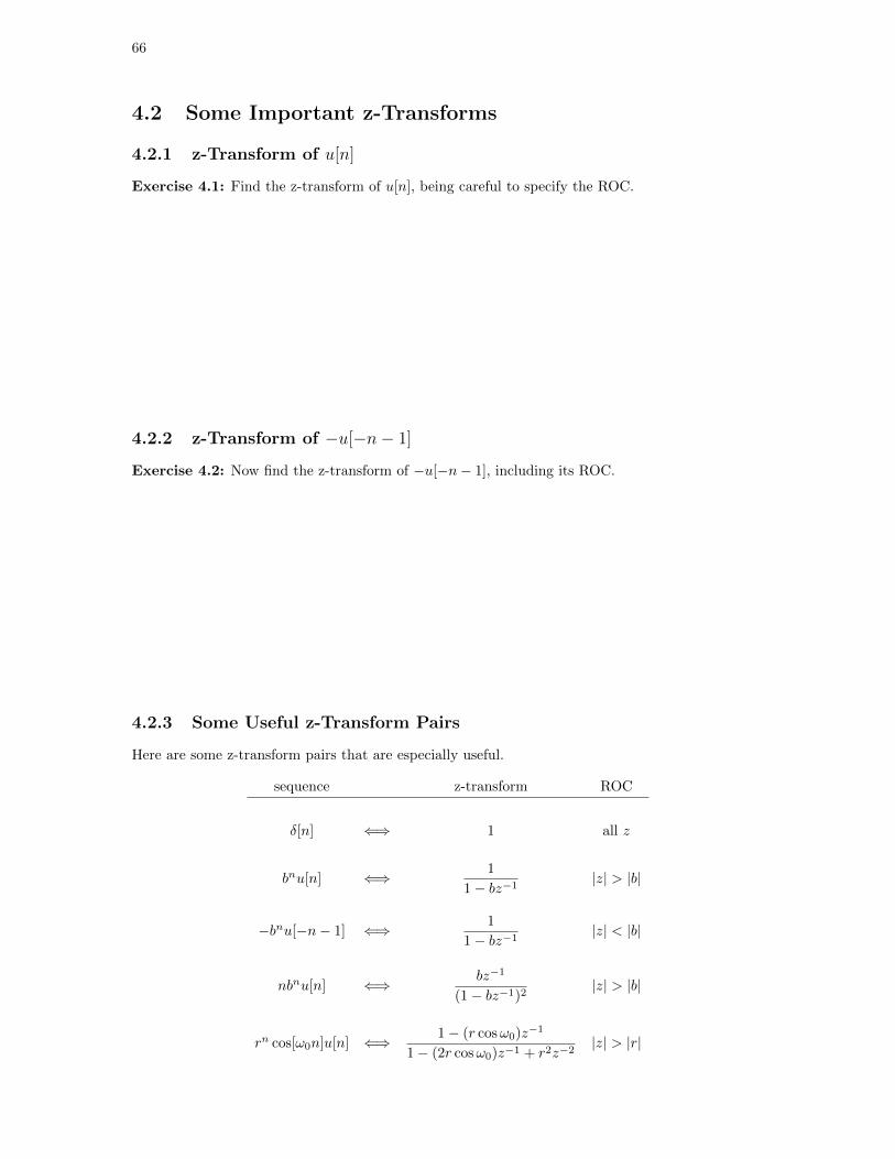
66

4.2 Some Important z-Transforms

4.2.1 z-Transform of u[n]

Exercise 4.1: Find the z-transform of u[n], being careful to specify the ROC.

4.2.2 z-Transform of −u[−n− 1]

Exercise 4.2: Now find the z-transform of −u[−n− 1], including its ROC.

4.2.3 Some Useful z-Transform Pairs

Here are some z-transform pairs that are especially useful.

sequence z-transform ROC

δ[n] ⇐⇒ 1 all z

bnu[n] ⇐⇒ 1

1− bz−1|z| > |b|

−bnu[−n− 1] ⇐⇒ 1

1− bz−1|z| < |b|

nbnu[n] ⇐⇒ bz−1

(1− bz−1)2|z| > |b|

rn cos[ω0n]u[n] ⇐⇒ 1− (r cosω0)z−1

1− (2r cosω0)z−1 + r2z−2|z| > |r|

M.C. Valenti Chapter 4. z-Transform 67

4.2.4 The z-Transform of Finite Sequences

Suppose that x[n] is nonzero only over the range N1 ≤ n ≤ N2 and zero elsewhere. The z-transform

is then:

X(z) =

N2∑n=N1

x[n]z−n = x[N1]z−N1 + ...+ x[N2]z−N2 . (4.126)

The ROC will include the entire z-plane except that z = 0 and/or z =∞ might not be in the ROC.

Exercise 4.3: Determine the z-transform of the folloiwing sequence:

x[n] = {1↑, 3, 2}.

Make sure to specify the ROC. For this transform, determine the values of z for which X(z) = 0.

These are the zeros of the transform.

Exercise 4.4: Let y[n] = x[−n], where x[n] is as specified in Exercise 4.3. Determine the z-

transform, including the ROC.

68

4.3 Computing the z-Transform with Matlab

Suppose we have a finite sequence x[n], which we may represent in matlab by the vectors x and

n. We would like to determine the z-transform. The key to doing this is to represent the complex

variable z in polar form,

z = rejω (4.127)

Substituting this into the definition of the z-transform, we get

X(z) =

∞∑n=−∞

x[n](rejω

)−n=

∞∑n=−∞

x[n]r−ne−jωn

=

∞∑n=−∞

(x[n]r−n

)e−jωn

= F{x[n]r−n

}(4.128)

This equation shows us that the z-transform evaluated at radius r is the DTFT of the modified

sequence x[n]r−n.

This suggests a method for computing the z-transform in Matlab if the sequence is finite.

1. Create a sampled frequency axis omega.

2. Create a sampled radius axis r.

3. For each value of r, determine the DTFT of the sequence x[n]r−n

The corresponding matlab code looks as follows:

NumFreq = 1000; % one less than the number of frequency samples

NumRad = 100; % number of radius samples

omega = 2*pi*[0:NumFreq]/NumFreq; % sampled frequency axis

MaxRad = 3; % maximum radius r

r = MaxRad*[1:NumRad]/NumRad; % the sampled radius axis

z = r’*exp(-j*omega); % the z-axis

for i=1:NumRad

X(i,:) = dtft( x.*r(i).^-n, n, omega ); % DTFT of modified signal

end

mesh( real(z), imag(z), 20*log10( abs(X) ) ); %visualize in 3-D

view(0,0); % look at it from the side.


4.4 Useful z-transform Properties

The z-transform has properties that are similar to that of the DTFT, namely:

Linearity: Z {ax[n] + by[n]} = aZ {x[n]}+ bZ {y[n]} = aX(z) + bY (z).

Sample Shift: Z {x[n− n0]} = z−n0Z {x[n]} = z−n0X(z).

Convolution: Z {x[n] ∗ y[n]} = Z {x[n]}Z {y[n]} = X(z)Y (z).

4.5 Convolution Using the z-Transform

Just as we can implement convolution by multiplying DTFT’s, we can also implement it by multi-

plying z-transforms.

Exercise 4.5: Using the z-transform, convolve the following two sequences:

x[n] = {5↑, 1, 3}

h[n] = {6↑, 4, 2}

70

4.6 System Function

The system function H(z) of a LTI system is the z-transform of its impulse response, i.e.

H(z) = Z {h[n]} . (4.129)

The frequency-response of the system is simply the system function evaluated at z = ejω.

Exercise 4.6: Consider a discrete-time system represented by a difference equation:

N∑k=0

aky[n− k] =

M∑k=0

bkx[n− k]. (4.130)

Determine an expression for the system function in terms of the coefficients {a0, ...aN} and {b0, ..., bM}.To do this, take the z-transform of both sides of (4.131) and solve for H(z) = Y (z)/X(z).

Exercise 4.7: Find the system function for the difference equation:

y[n]− 3

4y[n− 1] +

1

8y[n− 2] = x[n] + 3x[n− 1] + 2x[n− 2]. (4.131)

4.6.1 Poles and Zeros

Let H(z) = B(z)/A(z), then

• The poles of the system are the roots1 of the denominator polynomial A(z).

• The zeros of the system are the roots of the numerator polynomial B(z).

A pole-zero plot is a plot showing the locations of the poles and zeros on the complex plane. By

convention, poles are represented by ‘×’ and zeros are represented by ‘◦’.

1A root of A(z) is a value of z for which A(z) = 0.


Exercise 4.8: Determine the poles and zeros of the system specified by difference equation (4.132).

Sketch this system’s pole-zero plot. Hint: You may use Matlab’s roots function .

4.6.2 ROC and Poles

If a system is causal, then its impulse response is a right-sided sequence, and the region of convergence

of H(z) is

|z| > max |λk|

where λk are the poles.

Exercise 4.9: Determine the ROC for the system specified by difference equation (4.132).

4.6.3 Stability

Bounded-input, bounded-output (BIBO) stability requires that H(ejω) exists. This can only be true

if the ROC contains the unit circle. If the system is causal, then the ROC will be the region that

lies outside the outermost pole. Therefore, all poles must be inside the unit circle for the system to

be stable.

Exercise 4.10: Is the system with difference equation (4.132) stable?

72

4.6.4 Factored Form

Let {ξ1, ..., ξM} be the zeros of the system, and let {λ1, ..., λN} be the poles. The system function

may be written as:

H(z) =

(b0a0

) ∏Mk=1(1− ξkz−1)∏Nk=1(1− λkz−1)

=b0(1− ξ1z−1)(1− ξ2z−1)...(1− ξMz−1)

a0(1− λ1z−1)(1− λ2z−1)...(1− λNz−1)(4.132)

This is called factored form, and the quantity b0/a0 is called the system gain.

Exercise 4.11: Express the system function for the system with difference equation (4.132) in

factored form.

What happens when N 6= M?

We know that that if N > M , then there will be N −M extra zeros located at z = 0 and if M > N

there will be M −N extra poles located at z = 0. This is required to make the number of poles and

zeros the same. However, these extra poles or zeros are not apparent in equation (4.133), so where

are they? To reveal them, you need to express the system function in terms of z instead of z−1.

When N > M , this is done by multiplying the numerator and denominator of (4.133) by zN , which

results in

H(z) = zN−M(b0a0

) ∏Mk=1(z − ξk)∏Nk=1(z − λk)

. (4.133)

Similarly, if M > N , then multiply numerator and denominator of (4.133) by zM , which results in

the same expression as (4.134). The expression (4.134) is also a factored form of the system function.


Exercises

For each of the following difference equations, represent the system function in the factored form

given by (4.134). Furthermore, Sketch a pole-zero plot, and determine if the system is stable.

• Exercise 4.12: y[n] = x[n]−1.2x[n−1]+x[n−2]+1.3y[n−1]−1.04y[n−2]+0.222y[n−3].

• Exercise 4.13: y[n] = x[n]− 1.3x[n− 1] + 1.04x[n− 2]− 0.222x[n− 3] + 1.2y[n− 1]− y[n− 2].

4.6.5 Getting the Difference Equation from Poles and Zeros

If we are given the poles, zeros, and system gain b0/a0, we can immediately find the system function

in the factored form (4.133). If we would like to get the difference equation coefficients, then it is a

matter of converting the system function from the factored form into the polynomial form,

H (z) =

M∑k=0

bkz−k

N∑k=0

akz−k

. (4.134)

This can be accomplished in matlab by using the poly function.

74

Exercise 4.14: A system has system gain b0/a0 = 2 and the following set of poles and zeros:

ξk = {+1,+1}

λk =

{+

3

4,+

1

2

}Write out a difference equation for the system.

4.7 The Inverse z-Transform

The z-transform of a finite sequence x[n] = {x[N1], ..., x[N2]} is

H(z) =

N2∑k=N1

x[k]z−k (4.135)

and is easily inverted:

h[n] = Z−1{

N2∑k=N1

x[k]z−k

}=

N2∑k=N1

x[k]Z−1{z−k

}=

N2∑k=N1

x[k]δ[n− k]. (4.136)

But what if the sequence is not finite? How do you invert the z-transform? Oftentimes, it requires

a partial-fraction expansion.

4.7.1 Partial-Fraction Expansion

When there are no repeated poles and the sequence is causal, we can usually get by using the

following two z-transform pairs


bnu[n] ←→ 1

1− bz−1|z| > |b|

δ[n− k] ←→ z−k |z| > 0 if k > 0

along with the concept of partial-fraction expansion (PFE).


Exercise 4.15: Invert the following z-transform:

H(z) =1− z−1

1− 34z−1 + 1

8z−2 .

Note that this is a proper fraction (since the degree of B(z) is less than the degree of A(z)).

76

4.7.2 Dealing with Improper Fractions

Let H(z) = B(z)/A(z) be in rational form. Recall that M is the degree of B(z) and N is the degree

of A(z). If M ≥ N , then H(z) is an improper fraction. Before applying partial-fraction expansion,

it needs to be converted into the sum of a polynomial and a proper fraction through polynomial long

division.

H(z) = C(z) +B(z)

A(z)(4.137)

where C(z) is the quotient and B(z) is the remainder when B(z) is divided by A(z), i.e.

B(z) = C(z)A(z) + B(z). (4.138)

By performing a partial-fraction expansion on the proper fraction B(z)/A(z), H(z) may be expressed

as:

H(z) =

M−N∑k=0

Ckz−k

︸︷︷︸C(z)

+

N∑k=1

Rk1− λkz−1

. (4.139)

The direct-term polynomial C(z) is the quotient obtained by dividing B(z) by A(z), while Rk is the

residue associated with pole λk. Once the z-transform is expressed as given in (4.140), the inverse

z-transform is easily found as:

h[n] =

M−N∑k=0

Ckδ[n− k] +

N∑k=1

Rk (λk)nu[n]. (4.140)

Exercise 4.16: Invert:

H(z) =5− 4z−1 + 1

2z−2

1− 34z−1 + 1

8z−2 .


4.7.3 Inverting the Z-Transform in Matlab

Matlab can do the partial-fraction expansion for you. Just use the residuez function:

>> help residuez

RESIDUEZ Z-transform partial-fraction expansion.

[R,P,K] = RESIDUEZ(B,A) finds the residues, poles and direct terms

of the partial-fraction expansion of B(z)/A(z),

B(z) r(1) r(n)

---- = ------------ +... ------------ + k(1) + k(2)z^(-1) ...

A(z) 1-p(1)z^(-1) 1-p(n)z^(-1)

B and A are the numerator and denominator polynomial coefficients,

respectively, in ascending powers of z^(-1). R and P are column

vectors containing the residues and poles, respectively. K contains

the direct terms in a row vector. The number of poles is

n = length(A)-1 = length(R) = length(P)

The direct term coefficient vector is empty if length(B) < length(A);

otherwise,

length(K) = length(B)-length(A)+1

If P(j) = ... = P(j+m-1) is a pole of multiplicity m, then the

expansion includes terms of the form

R(j) R(j+1) R(j+m-1)

-------------- + ------------------ + ... + ------------------

1 - P(j)z^(-1) (1 - P(j)z^(-1))^2 (1 - P(j)z^(-1))^m

[B,A] = RESIDUEZ(R,P,K) converts the partial-fraction expansion back

to B/A form.

Exercise 4.17: Repeat the last two examples in Matlab using the residuez function.

78

4.7.4 Repeated Poles

If a particular pole λ has multiplicity m, then its terms are expanded as:

H(z) =

m∑`=1

R`

(1− λz−1)`

(4.141)

where

R` =1

(`− 1)!limz→λ

d`−1

dz`−1

((z − λ)

`H(z)

). (4.142)

To invert the first two terms of this summation, we can use the following z-transform pairs:


bnu[n] ←→ 1

1− bz−1|z| > |b|

(1 + n)bnu[n] ←→ 1

(1− bz−1)2|z| > |b|

If there are terms beyond this, they may be inverted by applying the differentiation property of the

z-transform. To keep things manageable, we will limit multiplicities in this class to be no more than 2.

Exercise 4.18: Determine the impulse response of the system described by difference equation:

y[n] +3

18y[n− 1]− 2

9y[n− 2]− 1

18y[n− 3] = x[n].


Exercise 4.19: Suppose that the input to the system given by Example 4.18 is:

x[n] =

{2↑, 1, 3

}.

Determine the output over the range 0 ≤ n ≤ 20. Find the output two ways: (1) Using the filter

function along with the difference-equation coefficients, and (2) Using the conv function along with

the impulse response.

80

4.7.5 Complex Poles

If a pole λ is complex, then the inverse z-transform Z−1{

1/(1− λz−1)}

= λnu[n] will produce a

complex-valued sequence. This is not the preferred representation of the output. Instead, we would

like the output to be expressed as a real-valued sequence. Fortunately, complex poles always occur

in conjugate pairs. Furthermore, the residues of a conjugate pair of poles are themselves a conjugate

pair. For each conjugate pair, there will be a pair of terms in the PFE of the following form:

H(z) =R

1− λz−1+

R∗

1− λ∗z−1(4.143)

which will have inverse z-transform:

h[n] = (R (λ)n

+R∗ (λ∗)n)u[n]. (4.144)

Recall that complex-valued residues R and poles λ can be represented as:

R = |R|ej∠R

λ = |λ|ej∠λ (4.145)

where |R| is the magnitude of R and ∠R is the angle of R, and similarly |λ| is the magnitude of λ

and ∠λ is the angle of λ. Thus we can express:

R (λ)n

+R∗ (λ∗)n

= |R|ej∠R(|λ|ej∠λ

)n+ |R∗|ej∠R

∗(|λ∗|ej∠λ

∗)n

= |R||λ|n(ej(∠R+n∠λ) + e−j(∠R+n∠λ)

)= 2|R||λ|n cos (∠R+ n∠λ) (4.146)

and it follows that the inverse z-transform for the conjugate pair of poles is:

h[n] = 2|R||λ|n cos (∠R+ n∠λ)u[n]. (4.147)

Exercise 4.20: Determine the impulse response of the system described by difference equation:

y[n]− 0.7y[n− 1] + 0.44y[n− 2] + 0.222y[n− 3] = 4x[n]− 3.24x[n− 1] + 0.928x[n− 2].

Express the impulse response as a real-valued sequence.


4.8 The poly Function

Suppose that instead of a difference equation or (polynomial form) system function, we are given a

set of poles and zeros along with the system gain b0/a0. We want to determine the impulse response.

The “b” coefficients can be found from the zeros, and the “a” coefficients can be found from the

poles. In matlab, the poly function will find the appropriate polynomial coefficients:

>> help poly

POLY Convert roots to polynomial.

POLY(A), when A is an N by N matrix, is a row vector with

N+1 elements which are the coefficients of the

characteristic polynomial, DET(lambda*EYE(SIZE(A)) - A) .

POLY(V), when V is a vector, is a vector whose elements are

the coefficients of the polynomial whose roots are the

elements of V . For vectors, ROOTS and POLY are inverse

functions of each other, up to ordering, scaling, and

roundoff error.

If the system gain is not equal to one, then simply multiply all the “b” coefficients by the gain.

Once the “a” and “b” coefficients are found, the system function can be inverted with the help of

the residuez function.

Exercise 4.21: Suppose a system has zeros

ξ =

{4

5,

3

5,

2

5,

1

5

}and poles

λ =

{3

4,

1

2,

1

4, 0

}and system gain b0/a0 = 2. Find the corresponding impulse response.

82

4.9 Problems

For the problems in this chapter, you may use matlab’s roots function or your calculator to determine

poles and zeros.

1. A particular discrete-time system can be represented by the following difference-equation:

y[n] +1

2y[n− 1]− 3

16y[n− 2] = x[n] + x[n− 1] +

1

4x[n− 2]

(a) Determine the system function, including the region of convergence.

(b) Determine the poles and zeros of this system.

(c) Is this system BIBO stable?

(d) Put the system function into factored form:

H(z) =

(b0a0

)((1− ξ1z−1)(1− ξ2z−1)

(1− λ1z−1)(1− λ2z−1)

)2. Determine the transfer function of each of the following causal LTI discrete-time systems

described by the difference equations. Express each transfer function in factored form and

sketch its pole-zero plot. Is the corresponding system BIBO stable?

(a) y[n] = 5x[n]+9.5x[n−1]+1.4x[n−2]−24x[n−3]+0.1y[n−1]−0.14y[n−2]−0.49y[n−3].

(b) y[n] = 5x[n]+16.5x[n−1]+14.7x[n−2]−22.04x[n−3]−33.6x[n−4]+0.5y[n−1]−0.1y[n−2]

−0.3y[n− 3] + 0.0936y[n− 4].

3. A causal LTI system has impulse response:

h[n] = n

(1

3

)nu[n] +

(−1

4

)nu[n].

For this system determine:

• The system function H(z), including the region of convergence.

• The difference equation.

• A list of poles and zeros along with the system gain b0/a0.

In addition, determine if this system is BIBO stable.


4. A causal linear time-invariant (LTI) discrete-time system has a pair of poles and a pair of

zeros. The poles are λ1 = 14 + j

√34 and λ2 = 1

4 − j√34 . The zeros are ξ1 = 0 and ξ2 = 1

4 . The

system gain is b0/a0 = 4.

(a) Is the system stable?

(b) Write the difference equation for this system using only real-valued coefficients. You may

assume that a0 = 1.

(c) The impulse response of this system may be written in the form:

h[n] = c (r)n

cos [ω0n]u[n]

Determine the values of the coefficients c, r and ω0.

(d) Suppose that the input to system is the sequence:

x[n] =

{4↑,−2, 1

}Determine the corresponding output sequence.

Chapter 5

Digital Filter Structures

5.1 The Implementation Problem

Now that we know how to design digital filters and represent them in a variety of ways (difference

equation, system function, impulse response), let’s turn our attention to implementation. Given a

desired filter, how do we implement in hardware or software? The key is to layout the system in the

form of a block diagram or signal-flow diagram.

5.1.1 Components

The components we have to work with are as follows:

Component Block Diagram Signal-flow Diagram

Multiplier

Delay

Adder

z-1

c

z-1

+

In this chapter, we will use signal-flow diagrams because they are more compact than block diagrams.

85

86

5.1.2 Goals

We will see that there is more than one way to layout a system. The goals of a good layout are:

Complexity: We would like to use the fewest number of components to achieve the desired design.

Stability: A system that is theoretically stable might become unstable when implemented. This is

because the filter coefficients must be quantized, so their values are slightly different than

anticipated. Each time a coefficient is quantized, there is a small amount of round-off error.

For large filters, the round-off error will accumulate to the point that poles might move outside

the unit circle.

5.2 Direct-Form I

Consider the difference equation:

N∑k=0

aky[n− k] =

M∑k=0

bkx[n− k]. (5.148)

Without loss of generality, set a0 = 1 and solve for y[n],

y[n] =

M∑k=0

bkx[n− k] +

N∑k=1

(−ak)y[n− k]. (5.149)

This equation can be directly realized with the following signal-flow diagram:

z-1

b0

z-1

.

.

.

.

.

.

.

.

.

.

.

.

b1

b2

bM

-a1

-a2

-aN

z-1

z-1

Such a system is called Direct-Form I or DF-I.

M.C. Valenti Chapter 5. Digital Filter Structures 87

5.3 Direct-Form II

Equation (5.150) can be rearranged as:

y[n] =

N∑k=1

(−ak)y[n− k] +

M∑k=0

bkx[n− k]. (5.150)

which may be realized as:

z-1

z-1

.

.

.

.

.

.

b0

b1

b2

bM

.

.

.

.

.

.

-a1

-a2

-aN

z-1

z-1

Notice in the figure that the same signal is delayed on both sides of the diagram. Thus, the

delays may be combined as follows:

.

.

.

b0

b1

b2

bM

.

.

.

.

.

.

-a1

-a2

-aN

z-1

z-1

Such a system is called Direct-Form II or DF-II. The benefit of DF-II over DF-I is that fewer delays

are required. For this reason, DF-I is hardly ever used.

88

5.4 Transposed Form

A signal-flow diagram can be transposed by reversing the direction of all arrows in the diagram. For

instance, the transposed DF-II structure is as follows:

.

.

.

b0

b1

b2

bM

.

.

.

.

.

.

-a1

-a2

-aN

z-1

z-1

Notice that when transposing, adders become branch nodes and vice versa. In addition, the input

and output become reversed. Since the usual convention is to put the input on the left side of the

diagram and the output on the right, we can reflect the diagram to get the following representation:

b0

b1

b2

bM

-a1

-a2

-aN

.

.

.

.

.

.

.

.

.

z-1

z-1

Note that other structures can be transposed, for instance DF-I.


Exercise 5.1: A causal LTI system is represented by the system function:

H(z) =1− 3z−1 + 11z−2 − 27z−3 + 18z−4

1 + 34z−1 + 1

8z−2 − 1

4z−3 − 1

16z−4 .

Draw the following structures:

1. Direct-form I.

2. Direct-form II.

3. Transposed direct-form II.

90

5.5 Cascade Form

Recall that a system function may be put into factored form:

H(z) =

(b0a0

) ∏Mk=1

(1− ξkz−1

)∏Nk=1 (1− λkz−1)

. (5.151)

The cascade form is an implementation that uses the factored form of the system function.

5.5.1 Cascade of First-Order Sections

For now assume that all poles and zeros are real-valued, that a0 = 1 and that N = M . Under these

assumptions, equation (5.152) may be expressed as:

H(z) = b0

M∏k=1

1− ξkz−1

1− λkz−1︸︷︷︸Hk(z)

(5.152)

which may be interpreted as the cascade of M first order sections. A high-level block diagram is as

follows:

!

1" #1z"1

1" $1z"1

!

1" #2z"1

1" $2z"1

!

1" #M z"1

1" $M z"1

… b0

The kth first-order section has transfer function:

Hk(z) =1− ξkz−1

1− λkz−1(5.153)

and difference equation:

y[n]− λky[n− 1] = x[n]− ξkx[n− 1]. (5.154)

When represented in DF-II form, the kth first-order section (FOS) is as follows:

-!k "k z-1

The overall signal-flow diagram is created by cascading M first-order sections, one after the other.


Exercise 5.2: Sketch the cascade form for the system described by the difference equation:

y[n]− 1.5y[n− 1] + 0.6875y[n− 2]− 0.09375y[n− 3]

= 2x[n]− 4x[n− 1] + 2.8x[n− 2]− 0.8x[n− 3] + 0.0768x[n− 4].

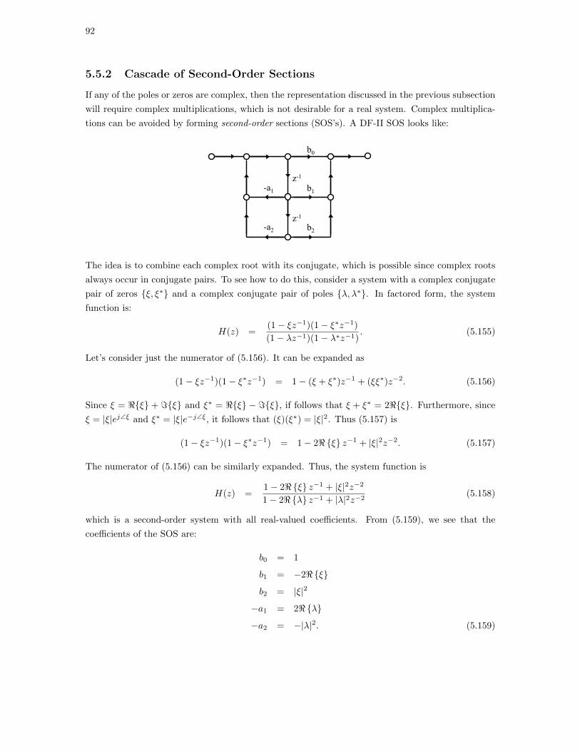
92

5.5.2 Cascade of Second-Order Sections

If any of the poles or zeros are complex, then the representation discussed in the previous subsection

will require complex multiplications, which is not desirable for a real system. Complex multiplica-

tions can be avoided by forming second-order sections (SOS’s). A DF-II SOS looks like:

b0

b1

b2

-a1

-a2

z-1

z-1

The idea is to combine each complex root with its conjugate, which is possible since complex roots

always occur in conjugate pairs. To see how to do this, consider a system with a complex conjugate

pair of zeros {ξ, ξ∗} and a complex conjugate pair of poles {λ, λ∗}. In factored form, the system

function is:

H(z) =(1− ξz−1)(1− ξ∗z−1)

(1− λz−1)(1− λ∗z−1). (5.155)

Let’s consider just the numerator of (5.156). It can be expanded as

(1− ξz−1)(1− ξ∗z−1) = 1− (ξ + ξ∗)z−1 + (ξξ∗)z−2. (5.156)

Since ξ = <{ξ} + ={ξ} and ξ∗ = <{ξ} − ={ξ}, if follows that ξ + ξ∗ = 2<{ξ}. Furthermore, since

ξ = |ξ|ej∠ξ and ξ∗ = |ξ|e−j∠ξ, it follows that (ξ)(ξ∗) = |ξ|2. Thus (5.157) is

(1− ξz−1)(1− ξ∗z−1) = 1− 2<{ξ} z−1 + |ξ|2z−2. (5.157)

The numerator of (5.156) can be similarly expanded. Thus, the system function is

H(z) =1− 2<{ξ} z−1 + |ξ|2z−2

1− 2<{λ} z−1 + |λ|2z−2(5.158)

which is a second-order system with all real-valued coefficients. From (5.159), we see that the

coefficients of the SOS are:

b0 = 1

b1 = −2<{ξ}

b2 = |ξ|2

−a1 = 2<{λ}

−a2 = −|λ|2. (5.159)


While SOS’s are essential for dealing with complex-valued roots, they can also be used when the

roots are real. The idea is to combine pairs of real-valued roots to form each SOS. For instance,

consider a system with a pair of real-valued zeros {ξ1, ξ2} and a pair of real-valued poles {λ1, λ2}.The system function is:

H(z) =(1− ξ1z−1)(1− ξ2z−1)

(1− λ1z−1)(1− λ2z−1)

=1− (ξ1 + ξ2)z−1 + ξ1ξ2z

−2

1− (λ1 + λ2)z−1 + λ1λ2z−2. (5.160)

The corresponding set of SOS coefficients are:

b0 = 1

b1 = −(ξ1 + ξ2)

b2 = ξ1ξ2

−a1 = (λ1 + λ2)

−a2 = −λ1λ2. (5.161)

It is also possible to have a SOS made up of a pair of real roots and a pair of complex poles, or

vice-versa.

Exercise 5.3: A particular causal system has system function:

H(z) =3− 9z−1 + 33z−2 − 81z−3 + 54z−4

1 + 34z−1 + 1

8z−2 − 1

4z−3 − 1

16z−4 .

Using a signal-flow graph, draw a cascade structure using second-order direct-form II sections.

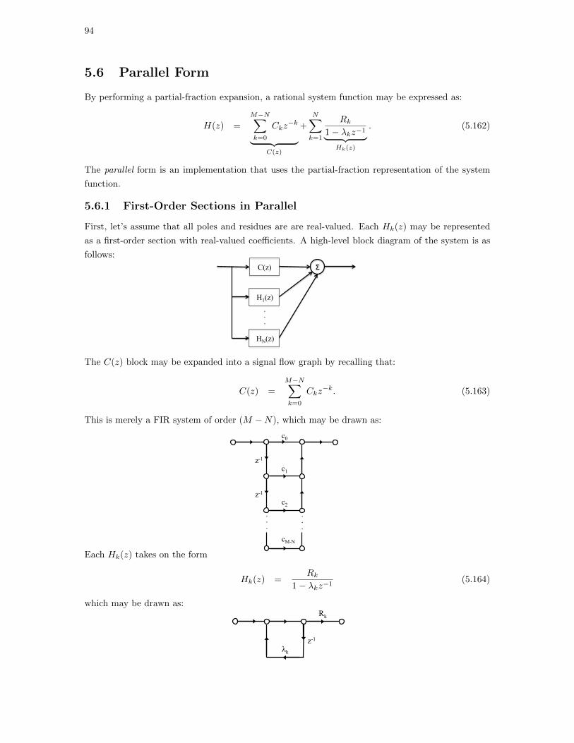
94

5.6 Parallel Form

By performing a partial-fraction expansion, a rational system function may be expressed as:

H(z) =

M−N∑k=0

Ckz−k

︸︷︷︸C(z)

+

N∑k=1

Rk1− λkz−1︸︷︷︸

Hk(z)

. (5.162)

The parallel form is an implementation that uses the partial-fraction representation of the system

function.

5.6.1 First-Order Sections in Parallel

First, let’s assume that all poles and residues are are real-valued. Each Hk(z) may be represented

as a first-order section with real-valued coefficients. A high-level block diagram of the system is as

follows:

C(z)

H1(z)

HN(z)

.

.

.

!

The C(z) block may be expanded into a signal flow graph by recalling that:

C(z) =

M−N∑k=0

Ckz−k. (5.163)

This is merely a FIR system of order (M −N), which may be drawn as:

z-1

z-1

.

.

.

.

.

.

c1

c2

cM-N

c0

Each Hk(z) takes on the form

Hk(z) =Rk

1− λkz−1(5.164)

which may be drawn as:

!k z-1

Rk



H(z) =5− 4z−1 + 1

2z−2

1− 34z−1 + 1

8z−2 .

Using a signal-flow graph, draw a parallel structure using first-order direct-form II sections.

96

5.6.2 Second-Order Sections in Parallel

If a pole or its residue is complex, then first-order sections will require complex multiplications, which

is not desirable. This can be avoided by joining complex poles and residues with their conjugates

to form second-order sections. Let λ be a complex pole and R its corresponding conjugate. We can

form a second-order section as follows:

R

1− λz−1+

R∗

1− λ∗z−1=

R(1− λ∗z−1

)+R∗

(1− λz−1

)(1− λz−1) (1− λ∗z−1)

=(R+R∗)− (Rλ∗ +R∗λ)z−1

1− (λ+ λ∗)z−1 + λλ∗z−2

=2<{R} − (Rλ∗ +R∗λ)z−1

1− 2<{λ}z−1 + |λ|2z−2(5.165)

where

Rλ∗ +R∗λ = 2|R||λ| cos (∠R− ∠λ) . (5.166)

This is a second-order section of the form:

b0

b1 -a1

-a2

z-1

z-1

where

b0 = 2<{R}

b1 = −2|R||λ| cos (∠R− ∠λ)

−a1 = 2<{λ}

−a2 = −|λ|2. (5.167)

Note that second-order sections can be used even when poles and residues are real-valued. Consider

a pair of real-valued poles {λ1, λ2} and their corresponding residues {R1, R2}. We can combine

them to form the second-order section:

R1

1− λ1z−1+

R2

1− λ2z−1=

R1(1− λ2z−1) +R2(1− λ1z−1)

(1− λ1z−1)(1− λ2z−1)

=(R1 +R2)− (R1λ2 +R2λ1)z−1

1− (λ1 + λ2)z−1 + λ1λ2z−2. (5.168)

The coefficients of the corresponding SOS are:

b0 = R1 +R2

b1 = −(R1λ2 +R2λ1)

−a1 = (λ1 + λ2)

−a2 = −λ1λ2. (5.169)



H(z) =3− 9z−1 + 33z−2 − 81z−3 + 54z−4

1 + 34z−1 + 1

8z−2 − 1

4z−3 − 1

16z−4 .

Using a signal-flow graph, draw a parallel structure using second-order direct-form II sections.

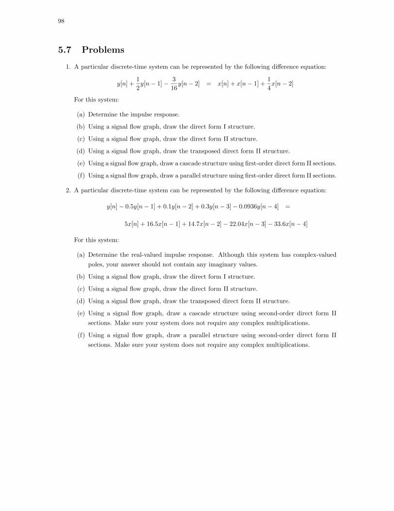
98

5.7 Problems

1. A particular discrete-time system can be represented by the following difference equation:

y[n] +1

2y[n− 1]− 3

16y[n− 2] = x[n] + x[n− 1] +

1

4x[n− 2]

For this system:

(a) Determine the impulse response.

(b) Using a signal flow graph, draw the direct form I structure.

(c) Using a signal flow graph, draw the direct form II structure.

(d) Using a signal flow graph, draw the transposed direct form II structure.

(e) Using a signal flow graph, draw a cascade structure using first-order direct form II sections.

(f) Using a signal flow graph, draw a parallel structure using first-order direct form II sections.

2. A particular discrete-time system can be represented by the following difference equation:

y[n]− 0.5y[n− 1] + 0.1y[n− 2] + 0.3y[n− 3]− 0.0936y[n− 4] =

5x[n] + 16.5x[n− 1] + 14.7x[n− 2]− 22.04x[n− 3]− 33.6x[n− 4]

For this system:

(a) Determine the real-valued impulse response. Although this system has complex-valued

poles, your answer should not contain any imaginary values.

(b) Using a signal flow graph, draw the direct form I structure.

(c) Using a signal flow graph, draw the direct form II structure.

(d) Using a signal flow graph, draw the transposed direct form II structure.

(e) Using a signal flow graph, draw a cascade structure using second-order direct form II

sections. Make sure your system does not require any complex multiplications.

(f) Using a signal flow graph, draw a parallel structure using second-order direct form II

sections. Make sure your system does not require any complex multiplications.

Chapter 6

The FFT

6.1 Motivation for Finite Transforms

Recall the expression for the DTFT:

X(ejω)

=

∞∑n=−∞

x[n]e−jωn. (6.170)

To compute the DTFT numerically (for instance, in Matlab), we had to sample the frequency axis

over a finite range of ω. In order to minimize complexity and storage requirements, we would like the

number of frequency samples to be as small as possible. Let’s now consider the problem of picking

the number of frequency samples in an intelligent way.

6.2 Discrete Fourier Series

Let x[n] be a periodic sequence with fundamental period N ,

x[n] = x[n+ kN ] (6.171)

for all k and all n. Let x[n], 0 ≤ n ≤ N − 1 be one period (the fundamental period) of the sequence

x[n]. Then x[n] can be represented by the discrete Fourier series (DFS)

x[n] =1

N

N−1∑k=0

X[k]W−nkN (6.172)

where

WN = e−j2π/N (6.173)

is called the nth root of unity, and

X[k] =

N−1∑n=0

x[n]WnkN (6.174)

are the DFS coefficients. Just as x[n] is periodic (with period N), so is X[k] (also with period N).

99

100

Exercise 6.1: Find the DFS coefficients for the sequence x[n] with fundamental period:

x[n] =

{3↑, 2, 1, 0

}.

6.3 Discrete Fourier Transform

Suppose that instead of a periodic sequence x[n], you have a finite sequence x[n] which is zero

outside the range 0 ≤ n ≤ N − 1. We can still find a DFS representation by “forcing” the signal to

be periodic. This is done by defining the periodic extension of x[n] to be

x[n] = x[n mod N ]. (6.175)

The discrete Fourier transform (DFT) of the finite signal x[n] is found from the DFS of its peri-

odic extension (in particular, the DFT is the fundamental period of the DFS of x[n]). The DFT

coefficients are:

X[k] =

N−1∑n=0

x[n]WnkN , (6.176)

which is a finite sequence defined over 0 ≤ k ≤ N − 1. The inverse DFT is:

x[n] =1

N

N−1∑k=0

X[k]W−nkN . (6.177)

As an example, the DFT of the sequence at the top of this page are the coefficients X[k] that form

the fundamental period of X[k].

M.C. Valenti Chapter 6. FFT 101

6.3.1 Relationship with DTFT

If you compare the equation for the DFT (6.177) with that of the DTFT (6.171), you will see that

X[k] = X(ejω)∣∣ω=k(2π/N)

=

∞∑n=−∞

x[n]e−jnk(2π/N)

=

N−1∑n=0

x[n](e−j(2π/N)

)nk=

N−1∑n=0

x[n]WnkN (6.178)

where the summation is only over 0 ≤ n ≤ N − 1 since x[n] is zero outside that range of n. Thus,

we may conclude that the DFT is merely the DTFT sampled at a frequency spacing of 2π/N .

6.3.2 Matlab Implementation

We can leverage our previous dtft function to come up with a dft function. Rather than passing

omega in as an argument, we will have the program itself determine an appropriate frequency axis.

Furthermore, rather than passing in n as an argument, we will assume that n ranges from 0 to N−1,

where N is the length of the sequence x[n].

function X = dft( x )

% Computes the DFT

% X = dft( x )

% where x = sampled signal defined over 0 <= n <= N-1

% X = the DFT coefficients

N = length( x );

n = 0:(N-1);

omega = n*2*pi/N;

X = dtft( x, n, omega );

102

6.4 The FFT Algorithm

The fast Fourier transform is an algorithm for efficiently computing the DFT. It performs best when

N is a power of 2. Matlab has a built-in fft function. As an exercise, compare the speed of our dft

function against that of Matlab’s fft function for a N = 212 = 4, 096 point transform.

N = 2^10;

tic;dft(rand(1,N));toc

tic;fft(rand(1,N));toc

Now compare the speed of fft for a N = 220 = 1, 048, 576 point transform against that of a N =

220 − 3 = 1, 048, 573 point transform:

N = 2^20;

tic;fft(rand(1,N));toc

tic;fft(rand(1,N-3));toc

As you can see, fft is not as efficient when N is not a power of 2, but it is still more efficient than

our dft function.

6.5 Circular Convolution

Consider two finite sequences x[n], y[n] and their periodic extensions x[n], y[n]. From the convolution

theorem of the Fourier transform, it follows that:

F {x[n] ∗ y[n]} = F {x[n]}F {y[n]} . (6.179)

Because the DFT is the DTFT of the periodic extension, it follows that

F {x[n] ∗ y[n]} = X[k]Y [k]. (6.180)

At first glance, this appears to have the usual relationship: That convolution in the time domain

corresponds to multiplication in the frequency domain. However, notice that we are not convolving

the two finite-length sequences x[n], y[n], but instead we are convolving their periodic extensions

x[n], y[n]. Such an operation is called a circular convolution. In matlab, circular convolution is

implemented with the cconv function.


Exercise 6.2: Circularly convolve the following sequences:

x[n] =

{1↑, 2, 0, 1

}y[n] =

{2↑, 2, 1, 1

}Do this in both the time domain (using cconv) and in the frequency domain (using fft and ifft).

104

6.5.1 Linear Convolution Using the FFT

Recall normal linear convolution of two finite sequences, i.e. x[n] ∗ y[n]. If x[n] has a length of N1

and y[n] has a length of N2, then the result of the convolution will have a length of N = N1 +N2−1.

It follows that linear convolution can be implemented from circular convolution (and hence, the fft),

if both sequences are zero padded out to a length of N .

Exercise 6.3: Using the FFT and zero-padding, linearly convolve the sequences given in the last

exercise.


6.5.2 Filtering with the FFT

The FFT gives an alternative way to implement a digital filter. The idea is that you first take the

FFT of the input sequence. Next, you multiply the transformed signal by the desired frequency

response. Finally, you take the inverse FFT.

Exercise 6.4: In this example, we have a signal x[n] = ne−0.03n, 0 ≤ n ≤ 255, corrupted by noise,

which we would like to filter:

n = 0:255;

x = n.*exp(-0.03*n); % desired signal

y = x + randn(size(x)); % noisy signal

figure(1);plot(n,x); % let’s use plot instead of stem

figure(2);plot(n,y); % since it is a long sequence

X = fft(x);

Y = fft(y);

figure(3);plot( abs(X) );

figure(4);plot( abs(Y) );

H = [ones(1,15) zeros(1,226), ones(1,15)]; % the filter response

Z = Y.*H; % filter in frequency domain

z = ifft( Z );

figure(5);plot(n, real(z) );

106

6.6 Problems

1. Determine the DFS coefficients of the following periodic sequences using the DFS definition,

(a) x1[n] = {2, 0, 2, 0}, N = 4.

(b) x2[n] = {0, 0, 1, 0, 0}, N = 5.

(c) x3[n] = {3,−3, 3,−3}, N = 4.

(d) x4[n] = {j, j,−j,−j}, N = 4.

This problem should be done with paper-and-pencil, but you may verify your answers in matlab.

2. Note: this problem should be done in matlab. A 12 point sequence x[n] is defined as

x[n] = {1, 2, 3, 4, 5, 6, 6, 5, 4, 3, 2, 1}

(a) Determine the DFT X(k) of x[n]. Plot (using the stem function) its magnitude and

phase.

(b) Plot the magnitude and phase of the DTFT X(ejω) of x[n] using matlab.

(c) Verify that the above DFT is the sampled version of X(ejω). It might be helpful to

combine the above two plots in one graph using the hold command.

the dsp workbook - west virginia...

Documents