This draft was prepared using the LaTeX style file belonging to the Journal of Fluid Mechanics 1

The effect of geometry on resistance inelliptical coaxial pipe flows

J.G. Williams1, B.W. Turney2, D.E. Moulton1, and S.L. Waters1∗1Mathematical Institute, University of Oxford, Oxford OX2 6GG, UK

2Nuffield Department of Surgical Sciences, University of Oxford, OX3 9DU

(Received xx; revised xx; accepted xx)

This paper considers the significant role of cross-sectional geometry on resistance in co-axial pipe flows. We consider an axially flowing viscous fluid in between two long and thinelliptical coaxial cylinders, one inside the other. The outer cylinder is stationary, whilethe inner cylinder (rod) is free to move. The rod poses a resistance to the axial flow, whilethe viscous fluid poses a resistance to any motion of the rod. We show that the equationsfor flow in the axial direction – driven by a prescribed flux – and for flow within the cross-section of the domain – driven by the motion of the rod – decouple in the asymptoticlimit of small cylinder aspect ratio into axial Poiseuille flow and transverse Stokes flow,respectively. The objective of this paper is to calculate numerically the axial and cross-sectional resistances and to determine their dependence on cross-sectional geometry – i.e.,rod position and the ellipticities of the rod and bounding cylinder. We characterise axialresistance, first for three reduced parameter spaces that have not been fully analysed inthe literature: I) a circle in an ellipse, II) an ellipse in a circle, and III) an ellipse in anellipse of equal eccentricity and orientation, before extending our geometric parameterspace to determine the overall optimal geometry to minimise axial flow resistance forfixed cross-sectional area. Cross-sectional resistance is characterised via coefficients in aStokes resistance matrix and we highlight the interdependent effects of cross-sectionalellipticity and boundary interactions.

1. Introduction

Fluid flow in annular geometries is prevalent, found in a range of apparatuses from oilwells to surgical tools. Annular flows between a co-axial rod and outer cylinder motivatefundamental design questions, such as:

1) How to position the inner cylindrical rod to maximise axial flow?2) How will the inner rod move and rotate if free to do so?3) How do the answers to 1 and 2 depend on the cylinders’ cross-sectional shapes?

A specific medical application of our work is found in a minimally invasive surgicalprocedure for the removal of kidney stones, uretero-renoscopy. This involves the insertionof long fibres, working tools, used to destroy or capture stones, through a long cylindricalworking channel along which there is an axially flowing saline solution. A minusculecamera in the scope tip allows the surgeon to see inside the patient’s kidney and theaxially flowing fluid is required to clear the field-of-view and to open up the ureter,see Figure 1. The working channel lies within the cylindrical shaft of a ureteroscope,and another outer cylinder, an access sheath, surrounds the scope itself, allowing fluidto flow back out of the kidney. Minimising the flow resistance posed by the workingtools can increase flow through the working channel and subsequent surgical accuracy

∗ Email address for correspondence: waters@maths.ox.ac.uk

2

Axial flow

79 cm

Axial flow

Kidney

Access sheath

Working channel

Working tool

CameraLight

0.12 cm

Scope shaft

Q

Q

Figure 1: A photograph of an isolated Boston Scientific ureteroscope (left) with the tipof the scope circled and a zoomed-in schematic provided of the scope tip (right). Thescope lies within an access sheath, and a working tool sits inside the working channel. Acamera and a light are embedded in the scope wall. Dimensions of the scope shaft andworking channel are labelled.

by improving visibility within the kidney (Williams et al. 2019a). Minimising the flowresistance through the access sheath leads to lower kidney pressures during uretero-renoscopy (Williams et al. 2019b; Oratis et al. 2018) which is desirable as high pressureshave been linked to post-operative complications, such as sepsis (Wilson & Preminger1990). This application in particular motivates us to address questions of flow optimalityin the sense of achieving the maximum flow rate for a prescribed axial pressure drop andfixed cross-sectional area available for fluid flow. The possible design of elliptical accesssheaths, working channels, and working tools has been motivated by the ureteral openingresembling an ellipse (Bergman 1981) and channels with elliptical cross-sections beingrelatively easy to manufacture. Thus, we restrict attention to cylinders with ellipticalcross-sections. When designing an optimal device the ideal scenario would be to placethe inner cylindrical rod in the position that minimises axial flow resistance. A keyconsideration is whether the surrounding fluid would then resist changes to the innerrod position, or whether the device must be designed to constrain the inner rod to theposition that minimises axial flow resistance.

Our modelling framework comprises a solid cylindrical rod of mass m and effectiveradius Ri, rotating about, and moving in a direction perpendicular to, its longitudinalaxis, within a coaxial outer cylinder of equal length, L, and comparable radius, Ro,filled with an axially flowing viscous fluid of typical flow rate Q, density ρ, and dynamicviscosity, µ. We take the cross-sections of the rod and outer cylinder to be ellipses ofvarying eccentricities; this is both appropriate for our uretero-renoscopy application andallows us to investigate the effects of non-axisymmetry. Typical parameter values forureteroscopy irrigation, which will guide our analysis here, are listed in Table 1. Definingthe radius-to-length ratio of the rod as ε = Ri/L and the Reynolds number of the flowas Re = QLρ/µR2

i , the key parameters governing the behaviour of the fluid and theinner rod are ε2, ε2Re, and the ratio of fluid-to-rod mass multiplied by the reducedReynolds number, α−1 = (m/ρR2

iL)ε2Re. Using typical values presented in Table 1, wefind ε2 = O(10−5 − 10−6), ε2Re = O(10−1), and α−1 = (100). These suggest that fluidinertia is negligible while rod inertia is not. In this regime, we show that the axial fluid flowthrough the annular region and the cross-sectional flows induced by the perpendicularmovement and rotation of the rod can be decoupled into axial Poiseuille flow andStokes flow in the cross-section. The motion of the rod is determined by conservation

3

Symbol Value Unit

Scope insheath

Ro 1.9× 10−1 cmRi 1.6× 10−1 cmL 3.6× 101 cmm 6.1× 100 g

Tool inworkingchannel

Ro 6.0× 10−2 cmRi 2.2× 10−2 cmL 7.9× 101 cmm 1.1× 100 g

Fluidproperties

Q 1.0× 10−1 cm3/sρ 1.0× 100 g/cm3

µ 1.0× 10−2 g/cm s

Table 1: Table of typical parameter values for ureteroscopy irrigation. For a scope in asheath, Ro is a typical effective radius of the access sheath (11/13 F Navigator, BostonScientific; 1 F corresponds to three times the diameter in millimeters) and Ri and mare a typical effective radius of the scope shaft and its mass, respectively (LithoVue,Boston Scientific). For a tool in a working channel, Ro is a typical effective radius of theworking channel (LithoVue, Boston Scientific) and Ri and m are a typical effective radiusof a working tool and its mass, respectively (ZeroTip 3.0 F, Boston Scientific). Fluidproperties are those of water, and the flow rate Q follows typical bench-top experimentsof flow through a working channel (Williams et al. 2019a).

of linear and angular momentum, incorporating the hydrodynamic resistance exertedby the surrounding viscous fluid. Within this setup, our objective is to investigate thenature of the resistance, both the cross-sectional resistance to the motion of the innerrod and resistance to the axial flow, in terms of the geometry of the two cylinders. Toillustrate characteristic features of the flow and to investigate geometric effects, we willfocus primarily on three reduced parameter spaces, namely:

I) a circular rod inside an elliptical cylinder,II) an elliptical rod inside a circular cylinder, and

III) an elliptical rod inside an elliptical cylinder of the same eccentricity and orienta-tion.

We also briefly consider the generic ellipse in an ellipse case when determining the optimalgeometry to minimise axial flow resistance. The literature on viscous-dominated fluidflows through annular pipes is vast. A description of relevant literature is given below andsummarised in Table 2. As our primary concern is the effect of cross-sectional geometryon resistance, we have grouped references by geometry in Table 2, and have furtherdistinguished which previous works have studied axial versus cross-sectional flow andmotion of the inner rod.

1.1. Axial flow resistance

An analytical solution exists for the steady, fully-developed (Poiseuille) flow of a viscousfluid through an annular region formed by concentric circles (Lamb 1916). By employingconformal maps, analytical solutions have also been obtained in a domain boundedby non-concentric circles (Piercy et al. 1933; Heyda 1959; Sastry 1964; Shivakumar &Chuanxiang 1993; MacDonald 1982). Numerical solutions for the flow in these domains,

4

together with the corresponding wall shear stress distributions, have also been obtained(Redberger 1962; Ebrahim et al. 2013; Snyder & Goldstein 1965). These solutionsdemonstrate that the distance between the centres of the bounding circles significantlyaffects the velocity distribution, and that the total flux for fixed pressure drop increaseswith this metric. Analytical solutions for steady, viscous flow through annular ductsbounded by confocal ellipses (Piercy et al. 1933; Sastry 1964), and externally by anellipse and internally by a circle (with coincident centres) have also been determined byemploying conformal maps (Sastry 1964), although the dependence of the flow rate onthe geometry of the domain was not discussed. Shivakumar & Chuanxiang (1993) alsoconsidered a region bounded internally by a circle and externally by a concentric ellipseand noted a flux enhancement compared to cross-sections bounded by two concentriccircles or two confocal ellipses of the same cross-sectional area. Flow through an annularregion bounded by non-concentric ellipses or by an ellipse in a circle, which form keycomponents of our analysis, has not been previously considered (see Table 2).

1.2. Cross-sectional flow resistance

Two-dimensional Stokes flow between two circular cylinders has been well-studied(Jeffrey 1922; Jeffrey & Onishi 1981; Frazer 1926; Chwang & Wu 1975; Wannier 1950;Slezkin 1955). The dynamics of a viscous fluid confined in the gap between rotatingcylinders, i.e. Taylor-Couette flow, has many mechanical applications, e.g. to the lubri-cation of rotary bearing systems. Stokes flow due to a line rotlet (a rotating circularcylinder of infinitesimal radius) inside an elliptic cylinder was solved analytically byHackborn (1991). The results focussed on the resulting flow structure and it was foundthat the number of eddies in the cross-section produced by the line rotlet increasedapproximately linearly with the ratio of length to width of the outer elliptical cross-section. Hackborn (1991) postulated that the flow features generated by a line rotletinside a fixed elliptic cylinder are expected to persist when the line rotlet is replaced bya rotating circular cylinder. Stokes flow between rotating confocal ellipses has also beenconsidered (Saatdjian et al. 1994), and an analytical solution for the stream functionobtained using elliptical cylindrical coordinates. It was shown that for counter-rotatingellipses, two hyperbolic points appear in the flow.

As the elliptical eccentricity of the outer cylinder cross-section tends to 1, the domainapproximates one of parallel plates. The motion of a rod of circular cross-section rotatingand translating in Stokes flow between parallel plates has been studied numerically(Dvinsky & Popel 1987). The authors computed the position between the centreline andthe wall where the rod experienced the minimum translational drag. It was also found thatthe torque on a cylinder rotating between parallel plates is minimised when the cylinderis centred between the two walls. An asymptotic solution (for small gap between thecylinder and the walls compared to the cylinder radius) for a circular cylinder rotatingbetween parallel plates was obtained by Yang et al. (2013). It was shown that if thecylinder is centred between the two plates, rotation will only induce an opposing torque,whereas if the cylinder is offset from the centreline, there is an additional force parallelto the walls.

Two-dimensional Stokes flow in a bounded annular domain with a translating androtating inner rod has also been considered. Finn & Cox (2001) presented an analyticalsolution for the stream function for such a flow when both the inner rod and outer cylinderhave circular cross-sections. The biharmonic equation for the stream function was solvedwith complex variable methods. The motion of the cylindrical rod was prescribed as afunction of time, and the energy required to maintain the system in equilibrium wasdetermined. It was shown that the power input depends upon the position of the rod

5

and the prescribed motion. As the two cylinders approach each other, the power inputrequired to maintain all motions diverges. Cox & Finn (2007) considered multiple rodswith elliptical cross-sections moving inside a circular cylinder via numerical methods.In both Finn & Cox (2001) and Cox & Finn (2007) the fluid flow is quasi-static, withtemporal variation in the velocity field only occurring due to changes in domain geometry.

While the above works demonstrate the strong effect of geometry on rod motion, to ourknowledge the effect of geometry on an elliptical cylindrical rod translating and rotatinginside an elliptical cylinder has not been previously investigated. Due to the linearity ofStokes equations, the velocity field resulting from any prescribed translational motion(in any bounded or unbounded two or three-dimensional domain) can be calculatedby considering component motions directed along orthogonal axes and summing thecomponent solutions. The velocity field resulting from prescribed rotational motion inthese domains can also be considered separately, and for combined translational androtational motions the solution is obtained by adding the relative contributions. Byimplementing the Lorentz reciprocal theorem, it can be shown that the magnitudes of thehydrodynamic forces and torques on a particle moving in Stokes flow vary linearly withthe imposed translational and rotational velocities, respectively, and these relationshipscan be captured by the coefficients of two symmetric resistance tensors (Brenner 1962c,1963; Hinch 1972). An additional tensor characterises the interactions between translationand rotation that can occur when particle or domain symmetry is broken (Brenner1963; Hinch 1972). The general theory for the effect of finite domain boundaries onthe resistance tensors has been considered for the case where the particle is small incomparison to its distance from the boundary (Brenner 1962a,b).

In two-dimensions, the three resistance tensors can be formulated as a single resistancematrix. To illustrate this, consider a Cartesian coordinate system with orthogonal direc-tions i, j, and k. For a given prescribed translational velocity, dx/dt i + dy/dt j, anda prescribed angular velocity dθ/dt k, the resistance matrix provides the hydrodynamicforces Fx i, Fy j and hydrodynamic torque τz k via

Fx

Fy

τz

= −

Kxx Kxy Cx

Kxy Kyy Cy

Cx Cy Azz

dx/dt

dy/dt

dθ/dt

. (1.1)

The scalar matrix coefficients Kij for i, j = x, y in equation (1.1) characterise theresistive force in the i-direction due to motion in the j-direction, and equivalently, as thematrix is symmetric, the resistance in the j-direction due to motion in the i-direction.Coefficient Azz provides the linear relationship between a rotational motion in the cross-section and the resistive torque. Finally, coefficients Cx and Cy describe the couplingbetween translational and rotational motions, i.e., the rotation induced by translation(and vice versa). The coefficients are all functions of the geometry of the domain (andscale linearly with viscosity).

When considering translation without rotation, equation (1.1) reduces to[Fx

Fy

]= −

[Kxx Kxy

Kxy Kyy

][dx/dt

dy/dt

]. (1.2)

The eigenvectors and corresponding eigenvalues of the matrix in equation (1.2) are thedirections and magnitudes of the minimum and maximum resistance, respectively. Usingprinciples of energy dissipation, it can be shown that the eigenvalues must be positive.

6

This is proved for a three-dimensional particle of arbitrary shape moving in Stokes flowin Brenner (1962c).

As a simple example of the resistance matrix for two dimensional flows, consider thecase of concentric circles of inner radius b and outer radius a. Stokes equations can besolved analytically in this geometry for prescribed translational and rotational velocitiesof the rod (Slezkin 1955, pp. 135, 163). The resulting resistance matrix components, Kxx,Kxy, Kyy non-dimensionalised by µ, Azz by µb2, and Cx, Cy by µb, are

Kxy = Cx = Cy = 0, (1.3a)

Kxx = Kyy = 4π(1 + r2)/(1− r2 + (1 + r2) log r), (1.3b)

Azz = 4π/(1− (1/r)2), (1.3c)

where r = a/b. Due to the symmetry of the domain there is no coupling betweentranslation and rotation. Moreover, the two eigenvalues of the matrix in equation (1.2) aregiven by Kxx = Kyy, i.e. there is equivalent resistance in all directions such that both thetranslational and rotational resistance decreases monotonically as the ratio r increases.A resistance matrix of the form given in equation (1.1) has been used to describe themotion of a cylindrical rod of circular cross-section translating and rotating in Stokes flowbetween parallel plates (Dvinsky & Popel 1987). More recently, resistance matrices havebeen used to understand the interactions between swimming micro-organisms (Ishikawaet al. 2006) and to control the movement of aqueous particles (Btait et al. 2019).

1.3. Resistance as the rod approaches the wall

For the cross-sectional flow problem it is important to mention a complexity thatarises if we are to consider the limiting behaviour that occurs when the rod touchesthe bounding cylinder. At this point, an interesting paradox arises: the resistance tomotion in all directions tends to infinity; i.e., it will require infinite force to move therod in any direction, including away from, or along, the contacting boundary (Jeffrey& Onishi 1981). To address this paradoxical behaviour, it is worthwhile to considerthe problem of a rod rolling or sliding along a plane wall in Stokes flow, as this willapproximate the behaviour of a moving rod touching a bounding cylinder close to thepoint of contact. Even in this simplified scenario, theory detects a pathologic problemwith solutions to the incompressible Stokes equations at the contact point, indicating thenecessity for fluid compressibility or cavitation to limit the pressure drop across the pointof contact to a physically acceptable value. This results in an infinite lift force, opening aninterstice between the wall and the cylinder; the fluid dynamics through this narrow gapcan be studied through lubrication analysis (Merlen & Frankiewicz 2011). The creationof cavitation bubbles for a rotating cylinder near a proximal wall has been confirmedexperimentally (Seddon & Mullin 2006), and these findings indicate a physical necessityfor a small gap between a moving rod and bounding cylinder. Thus, in Section 4, wherewe discuss cross-sectional resistance, we limit to configurations where the rod is a locateda finite distance from the bounding cylinder. Fixing a finite distance for the rod fromthe boundary also prevents divergence of numerical code, as mesh elements will becomedegenerate at the point of contact. Within this framework, we seek the configurationthat maximises the minimum eigenvalue of the Stokes resistance matrix, as, for a giveninstantaneous velocity, it will require the least work to perturb the position of the rod inthe direction of minimum resistance. Rod positions that incur high resistance to imposed

7

z

x

y

j

i

k

Θ

Θ

X

X(t)

Γi

Γo

Ω

Flux Q

z = L

z = 0

Figure 2: A schematic of the set-up in a Cartesian coordinate system (x, y, z) withcorresponding coordinate directions i, j, k, where k is oriented along the common axisof the cylinders of length L. At z = 0 the flow is driven by a flux, Q. The boundariesof a cross-sectional slice of the cylinders are denoted Γi (inner) and Γo (outer), and thefluid-filled area between them is Ω. The inset figure shows a cross-sectional slice, wherethe position and orientation of the rod are given by X and Θ, respectively. The rod hastranslational velocity X and angular velocity Θ.

instantaneous velocities are of interest to optimal design, as motion of the rod away fromthese positions will be naturally retarded by the hydrodynamic forces imposed by thefluid, without the need to mechanically fix the position of the rod.

1.4. Paper summary

This paper is organised as follows. In Section 2 we describe the model set-up. Inthe regime in which both the aspect ratio of the cylinders and the reduced Reynoldsnumber are small, we show that at leading-order the axial and cross-sectional flows canbe decoupled into Poiseuille flow and Stokes flow, respectively. In Section 3 we solvethe axial flow equations and compute the flux for a given pressure drop as a functionof rod position and the cross-sectional shapes of the rod and bounding cylinder, withan aim to determine configurations that minimise axial flow resistance. We will firstconsider the three special cases I), II), and III), before extending, in Section 3.4, ourdiscussion of optimal axial flow to the full geometric parameter space of an elliptical rodin an elliptical cylinder with fixed area available for the fluid. In Section 4 we solve thecross-sectional Stokes flow equations and calculate the forces and torque exerted on therod by the surrounding viscous fluid when the rod undergoes a prescribed motion. Wecalculate the resistance matrix coefficients as functions of cross-sectional geometry anddetermine which configurations have high resistance to perturbations in the rod position.For circles in ellipses and for ellipses in ellipses of the same eccentricity and orientation,we find that the position of the rod that maximises the axial flow rate and compare thisto the position of highest minimal resistance. We conclude in Section 5.

2. Mathematical model

We consider an inner cylindrical rod which is free to move within a fluid-filled outercylinder. The rod is prescribed a small, instantaneous, translational motion in a direction

8

DescriptionExampleGeometry

Poiseuille flowStokes flow(rotation)

Stokes flow(translation)

Centred circlein circle

Lamb (1916) Lamb (1916)Frazer (1926);Chwang & Wu

(1975)

Offset circlein circle

Piercy et al.(1933); Heyda(1959); Sastry

(1964);Redberger

(1962); Ebrahimet al. (2013);

Snyder &Goldstein (1965);

Shivakumar &Chuanxiang

(1993)

Jeffrey (1922);Jeffrey & Onishi(1981); Wannier(1950); Slezkin(1955); Finn &

Cox (2001)

Finn & Cox(2001)

Fully offsetcircle in circle

MacDonald(1982)

N/A N/A

Centred circlein ellipse

Sastry (1964);Shivakumar

(1973)

Offset circlein ellipse

Hackborn (1991)(rod of

infinitesimalradius)

Centredellipse in

circle

Centredellipse in

ellipse

Piercy et al.(1933); Sastry

(1964) (confocalellipses)

Saatdjian et al.(1994) (confocal

ellipses)

Offset ellipsein circle

Cox & Finn(2007) (includingmultiple ellipse

case)

Cox & Finn(2007) (includingmultiple ellipse

case)

Offset ellipsein ellipse

Circlebetween

parallel platesN/A

Dvinsky & Popel(1987); Yanget al. (2013)

Dvinsky & Popel(1987)

Table 2: Summary of existing literature for relevant geometries.

9

perpendicular to, and a rotation about, its longitudinal axis. The subsequent motion ofthe rod is driven by the hydrodynamic forces exerted on the rod by the fluid. As the rodmoves, we assume that it remains coaxial with the outer cylinder. While the rod is ableto move in the direction perpendicular to its longitudinal axis, we assume that it does notmove axially. It is also able to rotate about its longitudinal axis. Both the translationaland angular velocities of the inner rod are constant along its length.

Both cylinders are of length L and have uniform elliptical cross-sections. The spacebetween the inner and outer cylinders is filled with an incompressible, Newtonian fluid ofviscosity µ and density ρ. Flow is driven by both an applied non-zero constant axial fluxand the motion of the cylindrical rod. We adopt a Cartesian coordinate system (x, y, z)with corresponding coordinate directions i, j, k, where k is oriented along the commonaxis of the cylinders and z = 0 is at the entrance to the annular region (See Figure 2).With subscripts i and o denoting the inner and outer cylinders, respectively, we take thecharacteristic radii of the cylinders to be

Ri =√Ai/π, Ro =

√Ao/π, (2.1a,b)

where Ai and Ao are the respective cross-sectional areas. We assume that Ri and Roare comparable and much smaller than L. We denote the annular boundaries of a cross-sectional slice of the cylinders as Γo and Γi, respectively. The coordinate position ofthe geometric centre of the inner rod is given by (X(t), Y (t), L/2), where X and Yare functions of time, and thus the position of the inner rod within the cross-section isX(t) = (X(t), Y (t)). The orientation of the major axis of the rod’s cross-section, withrespect to the x-axis, is given by Θ(t), also a function of time (Figure 2).

2.1. Dimensionless system

As motivated in Section 1, we are interested in a regime where fluid inertia is negligible.Thus, the fluid flow is governed by the Stokes and continuity equations. We define theaspect ratio of the rod to be ε = Ri/L 1 and non-dimensionalise the axial coordinateby L and the cross-sectional coordinates by Ri = εL. We assume a non-zero constant fluxQ is applied at z = 0 and thus, non-dimensionalise the axial velocity by characteristicvelocity scale W = Q/R2

i . We choose the pressure scaling P = (Wµ/Lε2) to balance theviscous terms in the Stokes equations and the cross-sectional force and torque are scaledby εLµW and ε2L2µW , respectively. The dimensionless Stokes equations are given incomponent form by

−px + ε2(uxx + uyy) + ε4uzz = 0, (2.2a)

−py + ε2(vxx + vyy) + ε4vzz = 0, (2.2b)

−pz + wxx + wyy + ε2wzz = 0, (2.2c)

ux + vy + wz = 0, (2.2d)

where we have adopted the subscript notation for partial derivatives. Due to the scalingfor velocity, the dimensionless flux scales to∫∫

Ω

w dΩ = 1, (2.3)

where Ω is the 2D region of the cross-section between the cylinders.

10

No-slip conditions at the surfaces of the inner and outer cylinder give the dimensionlessboundary conditions

u = X − Θ(y − Y ),

v = Y + Θ(x−X),

w = 0,

on Γi (2.4a-c)

and

u = 0, on Γo. (2.5)

To calculate X and Θ, where dots denote derivatives with respect to time, we considerconservation of linear and angular momentum for the inner rod which gives, in dimen-sionless form

X = αF (X, Θ, X, Θ), Θ = α′τ(X, Θ, X, Θ), (2.6a,b)

where F and τ are the hydrodynamic force in the cross-section and z-component ofthe torque exerted on the rod due to the motion of the fluid, obtained by integratingcontributions from the viscous pressure forces. Because the cylinders remain coaxial, τand F are the only non-zero force and torque components. The dimensionless constantsin equations (2.6a,b) are defined as

α = µL2/mW, α′ = R2iµL

2/IW, (2.7a,b)

where m and I are the rod mass and the moment of inertia about the rod axis,respectively, and α′ is the same size as α as I scales with R2

im. We note that α can berearranged to relate the fluid density to the material density of the inner rod multipliedby the reduced Reynolds number. As discussed in the introduction, we will consider theregime where this parameter is O(1). As dimensionless initial conditions for equation(2.6) we prescribe

X(0) = X , Θ(0) = Φ, X(0) = U`, Θ(0) = ω, (2.8a-d)

where X is the initial location of the rod’s axis in the (x, y) plane, Φ is its initialorientation angle, U is its initial velocity in a direction given by `, a unit vector inthe (x, y)-plane, and ω is its initial angular velocity about the z-axis. We assume X , U ,Φ, and ω are all O(1); due to the chosen non-dimensionalisations, this requires the initialimposed rod velocities to be ε times smaller than the axial velocity.

2.2. Asymptotic analysis

We take ε2 1 and seek expansions to our dimensionless variables of the forms

u = u0 + ε2u1 + · · · , p = p0 + ε2p1 + · · · (2.9a,b)

X = X0 + ε2X1 + · · · , Θ = Θ0 + ε2Θ1 + · · · . (2.9c,d)

Inserting (2.9a,b) into equations (2.2c), (2.2d) and equating O(1) terms gives

∇2⊥w0 =

dp0dz

, ∇⊥ · u⊥0 + w0z = 0, (2.10a,b)

where u⊥0 = u0 i + v0 j, and that dp0dz is independent of x and y follows from equations

(2.2a) and (2.2b) at leading order. To determine the cross-sectional velocity components,

11

u0 and v0, we consider equations (2.2a) and (2.2b) at O(ε2), and obtain the two-dimensional Stokes equations

∇2⊥u0 = p1x, ∇2

⊥v0 = p1y. (2.11a,b)

The leading-order flux condition is ∫∫Ω

w0 dΩ = 1, (2.12)

and leading-order boundary conditions are

u0 = X0 − Θ0(y − Y0),

v0 = Y0 + Θ0(x−X0),

w0 = 0,

on Γi (2.13a-c)

and

u⊥0 = 0 and w0 = 0, on Γo. (2.14a,b)

The equations of motion for the tool, (2.6), read at leading-order

X0 = αF 0(X0, Θ0, X0, Θ0), Θ0 = α′τ0(X0, Θ0, X0, Θ0), (2.15a,b)

where the leading-order expressions for the hydrodynamic forces and torque on the rodare

F 0 =

∫ 1

0

[∮Γi

σ0 ni ds

]dz, (2.16a)

τ0 =

∫ 1

0

[∮Γi

(x−X0)(σ0 ni) · j − (y − Y0)(σ0 ni) · i ds

]dz, (2.16b)

for

σ0 =[−(p0/ε

2 + p1)I + (∇u⊥0 +∇u⊥0 )T]. (2.17)

The leading-order initial conditions for the rod motion are

X0(0) = X , Θ0(0) = Φ, X(0) = U , Θ = ω. (2.18)

2.3. Leading-order solution

We seek a separable solution for w0 of the form

w0 = f(x, y)dp0dz

. (2.19)

Integrating equation (2.10b) over a cross-section of the fluid domain between the twocylinders, using equations (2.13) and (2.14), and applying the divergence theorem gives∫∫

Ω

w0z dΩ = 0. (2.20)

Inserting the form (2.19) and using the imposed flux condition (2.3), we conclude that

d2p0dz2

= 0→ dp0dz

= const., (2.21)

12

and it follows that

w0z = 0. (2.22)

Hence equation (2.10b) becomes

∇⊥ · u⊥0 = 0, (2.23)

and the governing equation for the axial fluid flow, (2.10a), is

∇2⊥f(x, y) = 1, (2.24)

with no-slip boundary conditions, equations (2.13c) and (2.14b),

f = 0, on Γi, Γo. (2.25)

Additionally, using the flux condition (2.3) we can solve for the constant pressure gradient

dp0dz

=

∫∫Ω

f(x, y)dΩ

−1 , (2.26)

and thus

w0 = f(x, y)

∫∫Ω

f(x, y)dΩ

−1 , (2.27)

combining (2.19) and (2.26).As p0 is constant within a cross-section it has no contribution to the leading-order

hydrodynamic force and torque given by equations (2.16). Additionally, the bracketedterms in equations (2.16) are independent of z, and hence equations (2.16) and (2.17) tocalculate the force and torque reduce to

F 0 =

∮Γi

σ0 ni ds, (2.28a)

τ0 =

∮Γi

(x−X0)(σ0 ni) · j − (y − Y0)(σ0 ni) · i ds, (2.28b)

for

σ0 =[−p1I + (∇u⊥0 +∇u⊥0 )T

]. (2.29)

Henceforth, we will drop leading-order subscripts. We will retain the subscript onthe only first-order term that appears in our leading-order system, p1, to differentiatethe first-order pressure that drives flow in the cross-section, equations (2.11), from theleading-order pressure that drives the axial flow, equation (2.10a).

2.4. Model summary and computational approach

Equations (2.24), (2.25), and (2.27) give rise to Poiseuille-flow, where the axial flowresistance, R(X, Θ), is equal to the constant pressure gradient required to maintain theaxial flow through the annular domain at unit flux. This is given by

R(X, Θ) =

∫∫Ω

f(x, y)dΩ

−1 , (2.30)

13

a function of domain geometry. We note that for any given flux,

Q(X, Θ) =1

R(X, Θ)

dp

dz, (2.31)

and so, once R(X, Θ) is determined via equation (2.30), we can compute Q(X, Θ) forany specified pressure gradient. Motivated by the urological application, in which it ismost natural to consider optimising flow rate for a given pressure drop, our approach inSections 3 and 3.4 will be to fix dp/dz = −1 as a model input and compute Q(X, Θ) andthe associated flow profile as primary outputs. In this view, minimising the resistance isequivalent to maximising the flux.

The equations governing the cross-sectional flow are the Stokes equations (2.11) andincompressibility (2.23), with no-slip boundary conditions (2.13a,b) and (2.14a). Asdiscussed in Section 1, the forces and torque on the inner rod, equations (2.28a,b), arelinearly related to the imposed velocities via resistance coefficients

F (X, Θ, X, Θ) = −[K(X, Θ)X +C(X, Θ)Θ], (2.32a)

τ(X, Θ, X, Θ) = −[Azz(X, Θ)Θ + Cx(X, Θ)X + Cy(X, Θ)Y ], (2.32b)

where K(X, Θ) is the two dimensional translation matrix and C(X, Θ) describes thecoupling between translation and rotation

K(X, Θ) =

[Kxx Kxy

Kxy Kyy

], C(X, Θ) =

[Cx

Cy

]. (2.33a,b)

The resistance coefficients in equations (2.33a,b) are also functions of domain geometry.We will compute these in Section 4. To explore the effect of geometry on both the axialand cross-sectional resistances we consider configurations I), II), and III), as introducedin Section 1. In each configuration, we will fix the cross-sectional areas of the cylindersto constrain the space available for fluid. We do this by setting the characteristic radiusof the outer cylinder (scaled by Ri) which we denote Ro. This reduces the parameterspace, allowing for full interrogation of the axial and transverse flows on X, Θ, and theshape of the elliptical cross-sections of the inner and outer cylinders. In Section 3.4, wewill consider a more complete optimisation problem for axial flow resistance, relaxingour previous restrictions on the considered elliptical geometries.

3. Axial flow

We begin by considering the effect of cross-sectional geometry on axial flow by solvingequation (2.24) subject to conditions (2.25) for varying ellipse cross-sectional geome-tries. Results were calculated numerically using an open-source finite element library,oomph-lib (Heil & Hazel 2006). Details on the numerical elements and mesh are providedin Section A.2.

Our objective is to explore how the flux is affected by the position and orientation ofthe inner rod, X and Θ, respectively, and the elliptical eccentricity of the cross-sections.The eccentricity is defined as

ei,o =√

1− (bi,o/ai,o)2, (3.1)

where ai,o and bi,o are the major and minor axes of the inner and outer cylinder,respectively. A zero eccentricity value therefore corresponds to a circle and e = 1 is

14

a slit of zero width and infinite length. For fixed characteristic radii, see equations (2.1),and given eccentricity, ei,o, we can calculate ai,o and bi,o

ai = (1− e2i )−1/4, bi = (1− e2i )1/4, (3.2a,b)

ao = Ro(1− e2o)−1/4, bo = Ro(1− e2o)1/4, (3.2c,d)

3.1. I) Circle in ellipse

In Figure 3a∗ we consider a circular rod (of dimensionless unit radius) inside a cylinderof elliptical cross-section (with characteristic radius Ro = 2). We vary the eccentricityof the outer cylinder’s cross-section while maintaining the cross-sectional area, usingequations (3.2) to determine the corresponding lengths of the major and minor axes.When, for each value of eo, the rod is located at the position that maximises flux (seeAppendix B), we find that the flux initially increases with eo. The maximum flux overall eo (data point (ii)) is nearly 50% higher than the flux for a circular outer cylinder ofthe same cross-sectional area (data point (i)). The eccentricity at which the maximumflux is achieved is eo ≈ 0.84 for Ro = 2. We might hypothesise that this coincides withthe value for eo where the rod and bounding cylinder match curvature at the cylinder’svertex, which we denote e? (Appendix B). However, for Ro = 2, e? ≈ 0.78, which is lessthan the eo value where maximum flux is achieved. In fact, in configuration (ii) in Figure3a, although hard to discern from the colourmap, the circular rod tangentially touchesthe elliptic cylinder in two locations. The colorbar in Figure 3a gives the magnitude ofthe axial velocity, and demonstrates that the maximum velocity within the cross-sectionis also larger in configuration (ii), than in either (i) or (iii).

3.2. II) Ellipse in circle

When considering an elliptical inner rod and circular outer rod (eo = 0), we can, dueto the rotational symmetry of the outer domain, fix X = (X, 0) and vary the innerrod’s position along the x-axis only, without loss of generality. Here, we fix Ro = 3, alarger cross-section to allow for a wider range of feasible positions and orientations forthe inner rod, and vary X, Θ, and ei. We find, as anticipated, that Q increases with Xfor all values of ei and Θ. Increasing ei can either increase or decrease Q depending onthe position and orientation of the inner rod. For example, when the rod is centred inthe outer cylinder – and the flux is independent of Θ due to the geometry of the domain– the largest flux is obtained when the rod is circular, and decreases with ei. This effectcan be seen for ei = 0, ei = 0.7, and ei = 0.9 oriented at Θ = π/2 in the inset plotin Figure 3b. In contrast, when the rod is sufficiently offset, the more eccentric rods atΘ = π/2 cause less obstruction near the centre of the channel, allowing for higher flow(see Figure 3b).

For a circular rod (ei = 0), we validate our numerical solution against the analyticalsolution for offset circles (Piercy et al. 1933)† (dashed black line in Figure 3b) in additionto confirming that our numerical solution approaches the limiting case of touching circles(MacDonald 1982) as X approaches 2 (black cross in Figure 3b).

In Sections 3.1 and 3.2, we have considered the particular cases where one of thecylinders has a circular cross-section. As anticipated, in both configurations, the maxi-

∗Figure 3a has previously appeared in Williams et al. (2019a), an endourological publicationto translate these relevant findings for a clinical audience.†As Piercy et al. (1933) presents a solution for the flow rate in terms of an infinite sum, we

truncate this sum to determine the flow rate (see Appendix A.3).

15

e⋆ ≈ 0.78

0 0.2eo 0.6 0.8

1.4

Q

(a)

I) Circle in ellipse

0

0.3

0.6

(i)

(ii)

(iii)

2.6

0 2.32X

8

12

16

20

24II) Ellipse in circle

X

(b)

eo ≈ 0.84

Figure 3: Dimensionless flow rate, Q with X = (X, 0), as a function of (a) eo, for ei = 0,Ro = 2, and (b) X, for eo = 0, Ro = 3. In (a), for each eo, the inner circle is locatedat the position that maximises the axial flux (see Appendix B). When eo = e?, theellipse matches curvature with the circle at the ellipse vertex. The colorbar provides themagnitude of the axial velocity. Figure (b) plots Q as a function of X for ei = 0 (blue)ei = 0.7 (red) ei = 0.9 (yellow) oriented at π/2. The inset plot provides a zoomed-in viewfrom X = 0 to X = 0.2. The dashed black line gives the analytical solution by Piercyet al. (1933) and the black cross the solution by MacDonald (1982) (see Table 2 for moredetails).

mum flux was achieved for a rod tangent to the outer boundary. Perhaps unexpectedly,Figure 3a demonstrated that the optimal configuration may not be one where theinner rod is tangent at a single point. We will explore this in more detail in Section3.4, where we will determine the true optimal geometry that maximises axial flux (forfixed area), relaxing all previous geometric restrictions. However, we will first consideranother reduced parameter space, namely elliptical rods in elliptical cylinders of the sameeccentricity and orientation; a configuration that allows for clear specification of the innerrod’s position, and a discussion of the effects of eccentricity as a single parameter.

3.3. III) Ellipse in ellipse

We now consider cylinders with elliptical cross-sections of the same eccentricities e =ei = eo and orientation (Θ = 0). We fix Ro = 2 and again seek configurations thatmaximise the flux∗.

To describe the position of the inner ellipse relative to the outer ellipse we first defineθ to be the angle between the major axis of the outer ellipse and a line connecting thecentres of the two ellipses, see Figure 4. The effective radii of the inner and outer ellipsesare then defined as

ri = aibi/

√a2i sin2 θ + b2i cos2 θ, ro = aobo/

√a2o sin2 θ + b2o cos2 θ. (3.3)

With these definitions, the maximum distance, dmax between the centres at an angle θ

∗It is worthwhile to note, when comparing flux values between different geometries, that inthis section and in Section 3.4, Ro = 2, so the space available for fluid flow is the same as inFigure 3a (a circular rod in an elliptical cylinder) but less than in Figure 3b (an elliptical rodin a circular cylinder) where Ro = 3.

16

φ = 0 φ = 0.5 φ = 1

θd = dmax

θ d

(a) (b) (c)

ro

ri

Figure 4: Schematic showing a sample geometry for e = 0.8, θ = π/4 and (a) φ = 0, (b)φ = 0.5, (c) φ = 1. The shaded ellipse is the cross-section of the rod.

(when the rod and the outer cylinder touch) is given by

dmax = ro − ri. (3.4)

From this we define an offset parameter, φ, that is the ratio of the distance between thecentres of the two ellipses at an angle θ and dmax,

φ = d/dmax. (3.5)

Thus, the domain is characterised by three parameters; the eccentricity, e ∈ [0, 1), theangle of offset, θ ∈ [0, π/2], and the relative offset, φ ∈ [0, 1] (see Figure 4).

In Figure 5a-d we fix e = 0.8 and θ = 0, and plot the velocity profiles (withcorresponding flux values indicated) for φ = 0.01, φ = 0.35, φ = 0.7, and φ = 0.99.We observe that Q increases with φ, a result previously known for e = 0 (Piercy et al.1933; Redberger 1962). The effects of θ and e on Q are less intuitive. In Figure 5e-hwe fix e = 0.8 and φ = 0.99 and vary θ, plotting the associated velocity colourmaps forθ = 0, θ = π/6, θ = π/3, and θ = π/2. The flux is largest for θ = 0 and smallest forθ = π/3 demonstrating, for the chosen parameters, non-monotonicity of Q with θ. Wevary e in Figure 5i -l for fixed θ = 0 and φ = 0.99. The flux is largest for e = 0.6 andsmallest for e = 0.9, also demonstrating, for the chosen parameters, non-monotonicity ofQ with e. For completeness, line-plots of Q as a function of independent variation of e,φ, and θ can be found in Appendix C.

In Figures 6a-c, we show surface plots of Q in (φ, θ) space for three different ec-centricities: e = 0, e = 0.7, and e = 0.9, respectively. Note that, as Q varies mostsignificantly with φ, we have restricted to 0.9 6 φ 6 0.99 to isolate the effects of θ ande. When e = 0 (Figure 6a), Q is independent of θ due to the rotational symmetry of thedomain, and increases monotonically with φ. For eccentric domains, e = 0.7 and e = 0.9(Figures 6b and Figures 6c, respectively), Q is minimal at an intermediate value of θand φ = 0.9 (the smallest φ value plotted). The maximum Q is seen in Figure 6b fore = 0.7, further validating the existence of a nonzero eccentricity value that maximisesflux, emax. This existence of a non-zero eccentricity at which flux is maximised may beof particular interest from an engineering design point of view (Williams et al. 2019a).However, it is noteworthy that the optimal eccentricity itself will change based on theouter geometry. We plot emax as a function of Ro in Figure 6d. As Ro → ∞, emax → 0.As Ro characterises the ratio between outer and inner cross-sectional areas, the limitas Ro → ∞ corresponds to a negligible obstruction within the channel, and hence, themaximum flux will be attained for a circular cross-section (Williams et al. 2019a).

In this section we have determined that for equal eccentricities and orientations of theouter and inner ellipses, there is a position for the inner ellipse and a non-zero eccentricityvalue that maximises flux. We note that this may not be the configuration that maximises

17

e = 0.8θ = 0Vary φ

e = 0.8φ = 0.99Vary θ

θ = 0φ = 0.99Vary e

(a) φ = 0.01 (b) φ = 0.35 (c) φ = 0.7 (d) φ = 0.99

(e) θ = 0 (f ) θ = π/6 (g) θ = π/3 (h) θ = π/2

(i) e = 0 (j ) e = 0.3 (k) e = 0.6 (l) e = 0.9

−2.58 2.58 −2.58 2.58 −2.58 2.58 −2.58 2.58

−2.58 2.58−2.58 2.58−2.58 2.58−2.58 2.58

−2 2 −2.05 2.05 −2.24 2.24 −3.03 3.03

Q = 0.77 Q = 0.92 Q = 1.34 Q = 1.83

Q = 1.61

Q = 1.68Q = 1.86

Q = 1.60Q = 1.64Q = 1.83

Q = 1.81 Q = 1.83

kmin

0

0.25

0.5

Figure 5: Dimensionless velocity colourmaps with flux values, Q, for ellipses of equaleccentricities and orientations. Here Ro = 2. Axes are in (x, y) coordinates and thesevary with eccentricity so that the available space for fluid flow is constant. Colourbarsreflect different velocity values within the domains. The direction of the axis of minimalresistance, kmin, is indicated by the dashed white line on each diagram. This will bediscussed in Section 4.Plots (a)-(d) show the effect of offset, φ, for e = 0.8 and θ = 0. Offset values are (a)φ = 0.01, (b) φ = 0.35, (c) φ = 0.7, and (d) φ = 0.99.Plots (e)-(h) show the effect of angular position, θ, for e = 0.8 and φ = 0.99. Angularposition values are (a) θe = 0, (b) θ = π/6, (c) θ = π/3, and (d) θ = π/2.Plots (i)-(l) show the effect of eccentricity, e, for φ = 0.99 and θ = 0. Eccentricity valuesare (a) e = 0, (b) e = 0.3, (c) e = 0.6, and (d) e = 0.9.

flux for all values of ei, eo, X, Y , and Θ, and we consider this global optimisation problemin more detail in the following section.

3.4. Optimal geometry for axial flow

When solving for axial flow in Section 3 we considered three reduced geometricparameter spaces: I) circle in ellipse, II) ellipse in circle, and III) ellipse in ellipse ofthe same eccentricity and orientation. We found, in each case, eccentricity values andpositions for the inner rod that maximised Q. In this section, we will relax all previousassumptions on ellipse eccentricity and explore finding a global optimal geometry forellipses of fixed cross sectional area, Ro = 2.

For all configurations previously considered, we demonstrated that axial flow resistancewas lowered by increasing the distance between the centres of the inner and outer ellipses.Intuitively, we might expect that the optimal configuration is one where the inner ellipsetouches the boundary of the outer ellipse and with matching curvature, i.e. when the inner

18

Q Q

φ θ φ θ

e =0 e = 0.7

(a)

0.95

0.9 π/2π/4

0

1.5

1.85

(b)

1.6

1.9

Q

φ θ

e = 0.9

1.2

1.8

0π/4

π/20.95

0.9

(c)

1.4

2

0.950.9 π/2

π/40

φ = 0.99, θ = 0

(d)

0.1

0.9

0.5

0.3

0.7

5Ro

2010 15

Figure 6: Surface plots (a)-(c) give the dimensionless flow rate, Q, as a function of bothoffset, φ, and angular position θ of the inner ellipse for three different eccentricity values:(a) e = 0, (b) e = 0.7, and (c) e = 0.9. Here Ro = 2.Plot (d) gives emax as a function of the characteristic radius Ro. The emax value iscalculated as the one that produces maximum flow over 100 values from 0.01 6 e 6 0.99for each radius ratio.

ellipse ‘hugs’ the outer (although this was shown not to be the case for configuration I inSection 3.1). This assumption enables a reduced parameter space that can be approachedanalytically (see Appendix D). In Figure 7a we show a surface plot of Q as a function ofeo and θ produced by this calculation. We see that a global maximum occurs at θ = 0 andeo ≈ 0.71 with corresponding Q = 2.62 (indicated by the red circle and correspondingflow profile Figure 7b). (At this maximum, we also have ei ≈ 0.45, Θ = 0.)

The optimal configuration in Figure 7a shows a nearly 40% improvement in flux overthe optimal configuration computed in Section 3.3. However, it is still not sufficient toclaim this as the global optimum for ellipse geometries. In fact, the results in Figure3a suggested that a ‘curve-hugging’ configuration may not be optimal. Motivated bythis, we relax assumptions about how the ellipses meet at the boundary and formulatean optimisation problem to traverse the full parameter space. To this end, we define avector, g, containing the five parameters governing the geometry of the domain

g = (ei, eo, X, Y,Θ)T . (3.6)

19

0.6

0

0.3

0

1

.5

2

.5

eoθ

0.8 1.6 2.4

00.5

1 π/2

π/4

(a)

(b) Optimal in (a)

(c) True optimal

Q = 2.62

Q = 2.80

Figure 7: A plot of Q as a function of eo and θ for Ro = 2. Here the inner ellipse touchesthe outer boundary tangentially at a single point, matching curvature. The red circleindicates the presence of a global maximum.

The boundaries of the inner and outer ellipses, Γi and Γo, are

xTAx = 0, xTBx = 0, (3.7a,b)

respectively, where xT = (x, y, 1) and matrices A and B are functions of g. Thus, weseek the solution to the optimisation problem

ming−Q, s.t. c > 0, (3.8)

where c is a vector of six non-linear constraints, dependent on A and B and hence g,that ensure Γi is enclosed by Γo (see Appendix E for more details). We solve equation(2.24) in FEniCS (Alnaes et al. 2015), and implement MATLAB’s optimisation routine,fmincon, to solve the optimisation problem (3.8) with an interior-point method fromeight randomly generated starting points in the feasible five-dimensional parameter space.As the optimisation routine seeks local minima, a multi-start approach allows for globaloptimisation. The optimal geometry found through this method is shown in Figure 7cwith a corresponding flux, Q ≈ 2.80. The geometric parameters, see equation (3.6), areg ≈ (0.68, 0.74, 1.49, 0, π/2)T . This global optimum gives a non-negligible (nearly 7%)increase in flux compared with the ‘curve hugging’ optimum. Indeed, rather than perfectlymatching the geometries at the boundary, the global optimal geometry is tangent to theouter boundary in two locations (this was also true in the results in Section 3.1.) It isinteresting to note that this divides the fluid domain into two separate regions, which maybe connected to previous results (Ranger 1994, 1996) that demonstrate flux enhancementthrough creating multiply connected regions. (Ranger 1996) provides a short discussion onthe mechanism whereby disconnected regions can lead to increased total flux, discussingthe distribution of flux-per-unit-area for flow through a circular pipe. As flux-per-unit-

20

area is low at the edge, removing these regions and replacing them with disconnectedareas of higher flux may lead to enhanced flow.

4. Cross-sectional flow

We now turn attention to the cross-sectional flow problem, governed by the Stokesequations (2.11), (2.23), and the no-slip conditions (2.13a,b) and (2.14a). The objectiveis again to explore the impact of cross-sectional geometry within the configuration spaceof I), II), and III); but here the question is how the geometry impacts the resistancecoefficients for cross-sectional rod motion.

We solve the equations numerically using a finite element method implemented inoomph-lib (Heil & Hazel 2006) (details in Section A.2), and subsequently compute thedimensionless forces and torque on the rod due to the surrounding fluid via equations(2.28). We validate our numerical solution by comparing with analytical solutions forgeometries where these are available in the literature.

We consider a cross-section of the domain illustrated in Figure 2 (i), where the rod isgiven a prescribed instantaneous velocity, X = (X, Y ) in the (x, y) plane and a rotation,Θ about the z-axis. The resulting forces and torques, F = (Fx, Fy) and τ , are linearly

related to (X, Y ) and Θ by a symmetric resistance matrixFx

Fy

τz

= −

Kxx Kxy Cx

Kxy Kyy Cy

Cx Cy Azz

X

Y

Θ

, (4.1)

as discussed in Sections 1.2 and 2.4. If Θ = 0 then[Fx

Fy

]= −

[Kxx Kxy

Kxy Kyy

][X

Y

]. (4.2)

The eigenvectors of the 2×2 matrix in equation (4.2) are the directions of minimum andmaximum opposing force experienced by the rod due to the flow. We will refer to theseas the directions of minimum and maximum resistance. The corresponding eigenvaluesgive the magnitudes of the opposing forces that result from moving in the directions ofminimum and maximum resistance with unit velocity. These values are non-negative (seeSection 1.2) and are given by

Kmax = (1/2)(Kxx +Kyy +

√(Kxx −Kyy)2 + 4K2

xy

), (4.3a)

Kmin = (1/2)(Kxx +Kyy −

√(Kxx −Kyy)2 + 4K2

xy

), (4.3b)

with corresponding directions of minimum and maximum resistance

kmax,min = (Kxy,Kmax,min −Kxx). (4.4)

21

The six unique scalars in the resistance matrix (4.1) can be computed by imposing:

X = (1, 0), Θ = 0, → Kxx, Kxy and Cx, (4.5a)

X = (0, 1), Θ = 0, → Kyy, Kxy and Cy, (4.5b)

X = (0, 0), Θ = 1, → Cx, Cy and Azz, (4.5c)

where each calculation provides us with the coefficients indicated by the arrows. We notethat Kxy, Cx, and Cy can each be determined by two separate calculations, and weperform both as validation (to within numerical error).

4.1. I) Circle in ellipse

The analytical solution for Stokes flow between concentric and offset circular cylindersdemonstrates a dependence of the forces and torque experienced by the rod on thegeometry of the domain (Finn & Cox 2001). We first consider how these results changewhen the bounding cylinder is elliptical. To limit the candidate geometries, we positionthe rod along the x-axis, i.e. X = (X, 0). We fix the cross-sectional area and set Ro = 2.

For a circular rod translating within a circular cylinder, Kxx and Kyy increase as therod approaches the edge of the bounding cylinder, and Kxy = 0, due to the symmetryof the domain (Slezkin 1955). As expected, we find that for eo > 0, the same behaviouroccurs. The effect of eo on the resistance coefficients is not quite so straightforward as theeffect of position – as eo increases for fixed X, the proximity of the rod to the boundaryin the vertical direction decreases while the distance to the boundary in the horizontaldirection increases, and at nonequal rates. Due to these competing features, Kyy exhibitsan interesting dependence on eo for X = 0. In Figure 8a, we plot Kyy as a function of eofor a centred rod, and we observe a non-monotonic behaviour, highlighting the complexityof boundary interactions. Comparing resistance coefficients for X 6= 0 adds yet anothercomplexity: as the range of feasible X values increases with eo (as long as the rod canstill fit tangent to the vertex of the outer cylinder), we can either compare values atabsolute, X, or relative, X/(ao− 1), distance from the centre, which qualitatively affectsthe observed trends. We find that, depending on the metric used, Kxx, Cy, and Azz canalso be non-monotonically related to eo when the cylinder is offset‡. We note that Cx = 0for a rod centred on the x-axis, due to arguments of symmetry.

If, instead of fixing cross-sectional area, we fix the gap between the rod and the cylinder,the domain approaches one of a rod between parallel plates as eo → 1. An asymptoticapproximation to the Stokes force and torque on a cylinder rotating between parallelplates was obtained by Yang et al. (2013), where the ratio of gap width to cylinderradius defines the small parameter, ε. To test whether the resistance coefficients for a rodin an elliptic cylinder approach those for a rotating rod between parallel plates (Yanget al. 2013), we consider a rod at X = 0 in an elliptic cylinder of fixed minor axis,bo = 1.025, which sets the gaps between the rod and the cylinder at x = 0, to be 0.025.In Figure 8b we plot Azz as a function of outer eccentricity (line ii), and we see that aseo → 1 the resistance approaches the value for parallel plates with ε = 0.025 (Yang et al.2013) (line i). As we increase eo with fixed minor axis, the cross-sectional area of theelliptic cylinder is also increasing. Thus, as a further geometric comparison, line iii plotsAzz for a rod centred in a circular cylinder with increasing and equivalent cross-sectionalarea (i.e. for each eo, the bounding circle has cross-sectional area equal to that of anellipse of eccentricity eo and minor axis bo = 1.025). Although Azz decreases with eo due

22

120

0 0.3 0.6 0.9eo

Kyy

160

200

240(a)

200

100

250

50

00.2 0.4 0.6 0.8 10

Azz

i

ii

iii

eo

iiiǫ ǫi ii

(b)

Figure 8: Results for Ro = 2. (a) Rod translating with unit velocity in the y-direction,centred at (0, 0). Kyy is plotted as a function of eo. Inset schematics are for (left-right)eo = 0, eo = 0.63, and eo = 0.9 (b) Plot of Azz for a circular rotating rod centred at(0, 0). The rod is rotating: (iv) between parallel plates with gap size ε = 0.025 (Yanget al. 2013) (v) within an outer elliptic cylinder with bo = 1.025 (Ro not fixed) (vi)within an outer circular cylinder of radius Ro = 1.025(1 − e2o)−1/4. Solution obtainedfrom equation (1.3c).

to the increase in cross-sectional area available for the fluid, Azz is larger when the outerboundary is an ellipse compared to a circle of the same cross-sectional area.

4.2. II) Ellipse in circle

The next domain we consider is an ellipse in a bounding circle. As in Section 3.2, dueto the rotational symmetry of the outer domain, the number of unique combinationsof position and orientation of the rod can be reduced; it is sufficient to consider therod centred at X = (X, 0) and to vary X, Θ, and ei. In Figure 9 we investigate howthe resistance coefficients are influenced by the shape of the rod’s cross-section and itsorientation and proximity to the outer boundary. In Figure 9a-c, results are plotted asfunctions of absolute offset, and the orientation of the rod, Θ, as well as its position, X,determine the proximity of the boundary, and in a non-trivial way.

We first consider resistance to rotation. We find that Azz increases as a functionof offset for fixed ei and Θ. Results are shown in Figure 9a for three eccentricities,ei = 0, ei = 0.7, and ei = 0.9, oriented at Θ = 0, Θ = π/4, and Θ = π/2. Forfixed position and orientation, rotational resistance increases with eccentricity. Withoutboundary interactions, Azz would be independent of Θ; however due to the presence ofthe bounding circular cylinder, for moderate X 6= 0, Azz is largest when Θ = π/2 andsmallest when Θ = 0. As evidenced by the crossing lines for ei = 0.9 in Figure 9a, whenX is sufficiently large, a rod oriented at Θ = 0 receives the largest opposing torque, whichis likely due to the proximity of the vertex of the major axis to the boundary. We notethat, if we increase the X range in Figure 9a, this effect is also seen for ei = 0.7‡.

Turning now to translational resistance, our results validate the intuition that whenthe major or minor axis of the rod’s cross-section is aligned both with the direction ofmotion and a radial line of the outer cylinder’s cross-section, the force on the rod actsparallel to its direction of motion, and the lift force is zero. Brenner (1962a) proved thisto be true for the motion of a bounded arbitrary particle.

‡Results shown in Appendix F.

23

Azz

ei = 0

ei = 0.7

ei = 0.9

Slezkin (1955)

0 0.4 0.8 1.2 1.410.60.2X

0

5

10

15

20

25

30

15

25

35

45

55

65

0 0.4 0.8 1.2 1.410.60.2X

Kxy

(a)

K

30

50

70

90

110

0 0.4 0.8 1.2 1.410.60.2X

(c)

Kxx

Kyy

Kmin

−30

−20

−10

0

10

ei

3Cy

ei = 0 0ei = 0

p1−3

3

0 0.3 0.6 0.9

(d)

ei = 0.7

(b)

Figure 9: Figure (a) and (b) give Azz and Kxy, respectively, as functions of X for ei = 0,ei = 0.7, and ei = 0.9 and Θ = 0, Θ0 = π/4, and Θ = π/2. In (b), Kxy is identicallyzero for Θ = 0 and Θ = π/2, so these are not shown as they coincide with the line forei = 0. Figure (c) displays Kmin for Θ = 0 and ei = 0, ei = 0.7, and ei = 0.9. Figure (d)gives Cy as a function of ei for Θ = 0 and X = 1.45. Colormaps of pressure p1 near thebounding wall, due to an imposed angular velocity, are shown for ei = 0 and ei = 0.7with the colorbar providing the magnitude of p1, centred around p1 = 0. All plots havea dimensionless outer radius of Ro = 3.

Of the three translational resistances, we first consider the lift force, Kxy. We find, thatfor fixed ei andX away from the boundary,Kxy is maximised for Θ = π/4. Thus the outercylinder does not seem to change classic results for an elliptic cylinder in an unboundedfluid (Lee & Leal 1986). To see how the lift force changes with inner eccentricity, inFigure 9b we fix the orientation at the maximal value Θ = π/4 for eccentricities ei = 0,ei = 0.7, and ei = 0.9, and plot Kxy as a function of X. We find a significant increase inlift force with eccentricity, and also a non-monotonic relation with position in the caseof ei = 0.9.

Next, we analyse Kxx, Kyy, and Kmin. For relatively small offset, Kxx is smallest (andKyy largest) when Θ = 0. We restrict to this orientation, and plot Kxx (dotted line)and Kyy (dashed line) as functions of X for ei = 0.7 and ei = 0.9 in Figure 9c. Aninteresting feature is the non-monotonic behaviour of Kyy with X. The solid colouredlines give the value of the minimum resistance, Kmin. Looking particularly at ei = 0.9we see that for small values of X, Kmin coincides with Kxx (and thus the eigenvectorkmin = ex). However, near X = 1.2 the lines Kxx and Kyy cross, and the direction ofminimum resistance switches to be aligned with the y-axis. The same behaviour is seenfor ei = 0.7, with the switching occurring at a smaller offset (near X = 1). The solid

24

lines denoting Kmin for each eccentricity also cross. When X is small, Kmin is largest forei = 0 and smallest for ei = 0.9 and vice versa for large X. Again, this can be explainedby the significance of boundary interactions: far from the boundary the more eccentricellipse has a direction of small resistance – its major axis – but closer to the boundarythe major vertex is in closer proximity to the boundary, compared to ellipses of smallereccentricity, hence the resistance in both the x- and y-directions rapidly increases. Wehave also demonstrated that for Θ = π/2, kmin is aligned with the y-axis for ei = 0,ei = 0.7, and ei = 0.9 (at least for 0 6 X 6 1.45)‡.

Finally, we consider the coupling between translation and rotation. We find, for fixedei and X away from the boundary, Cx is largest for Θ = π/4 and Cy is largest forΘ = π/2‡. When the rod is oriented at Θ = 0, there is coupling between rotation andtranslation in the y-direction (Cy 6= 0). This is known analytically for ei = 0 (Slezkin1955), and in this classic case, Cy increases monotonically with X. Interestingly, formore eccentric ellipses, this is no longer true; in fact, Cy can change sign as a functionof position along the X-axis. Alternatively, this behaviour can be illustrated by plottingCy as a function of eccentricity for fixed X sufficiently close to the outer boundary. Thisis shown in Figure 9 for X = 1.45 (the furthest-right position in Figures 9 (a)-(c)). Weobserve that Cy decreases as a function of ei, changing sign from positive to negative. Toexplain this behaviour, consider a rotating rod with imposed angular velocity, in whichcase Cy characterises the induced translational force in the y-direction. Example pressureprofiles for ei = 0 and ei = 0.775 near the proximal boundary are shown in the insets, andthese show that the pressure drop in the lubrication layer between the rod and the outerboundary changes direction as a function of ei. Due to the proximity to the boundary,we can appeal to Reynolds’ lubrication equation to understand this inversion in termsof the behaviour of the fluid in the lubrication layer: for a circular surface rotating neara fixed plane, the pressure drop is in the opposite direction compared to the pressuredrop for a highly curved surface moving parallel to the plane (Wannier 1950). For oursystem, rotating an ellipse of high eccentricity is analogous to moving the vertex (andpoint closest to the boundary) parallel to the boundary, whereas rotating an ellipse ofsmall eccentricity does not change significantly the minimal distance to the boundaryand hence behaves more like a rotating circle.

4.3. III) Ellipse in ellipse

In this section we revisit the configuration considered in Section 3.3, with both therod and bounding cylinder having elliptical cross-sections of the same eccentricity, e, andorientation (Θ = 0). We set Ro = 2, and parameterise X by offset φ and angular positionθ, illustrated in Figure 4. Returning to Figure 5, the direction of minimum resistance ismarked with a dashed white line. We see that when the rod is centred in the outercylinder, kmin lies along the major axis of the ellipse. As we move towards the wall, thisdirection switches to the minor axis, due to the build-up of pressure between the rodand the proximal edge of the outer cylinder. As we break symmetry and vary θ, kmin nolonger lies along an axis of symmetry of the inner ellipse and for φ = 0.99 it varies fromvertical for θ = 0 to horizontal for θ = π/2, see Figures 5 (e)-(g).

Figures 6a-c showed the axial flow rate in the (φ, θ) parameter space for three differenteccentricity values, and in Figure 10a-c, we plot Kmin for the same domains. For bothe = 0.7 and e = 0.9, the smallest value of Kmin occurs at θ = π/2 and an intermediateφ value 0 < φ < 1. Here Kmin is in the x-direction, aligned with the major axis of therod. This is similar to the behaviour determined by Dvinsky & Popel (1987) of a circularcylinder translating between two plates, parallel to the boundaries, where the lowest forcewas incurred at a position between the centreline and the wall, with the exact location

25

0 0.2 0.4 0.6 0.8 1e

122

126

130

134

138

600

1000

1400

1800

0 0.2 0.4 0.6 0.8 1e

π/2π/4

0

00.5

1200

400

600

π/2π/4

0

00.5

1

600

200 500

1000

1500

π/2π/4

0

00.5

1100

200

300

400

500

θ

Kmin

e = 0

(a)

θ

400

e = 0.7

θ

e = 0.9

(b) (c)

(d) (e)

min(Kmin)max(Kmin)

φ φ φ

Figure 10: Surface plots (a)-(c) give the value of Kmin as a function of both offset, φ, andangular position θ (where these values are defined as in Section 3) of the inner ellipse forthree different eccentricity values: (a) e = 0, (b) e = 0.7, and (c) e = 0.9.Plots (d) and (e), respectively, show the maximum and minimum value of Kmin givesthe minimum value of Kmin for a given equal inner and outer ellipse eccentricity value.The geometries that provide the min(Kmin), (d), and max(Kmin), (e), for e = 0, e = 0.4,e = 0.7, and e = 0.9 are demonstrated by diagrams and the white-dashed line on each ofthese shows the direction of minimum resistance. Ro = 2.

being dependent upon the ratio of the radius of the cylinder to the distance between thewalls.

In Figure 10d, the minimum value of Kmin over (φ, θ)-space is plotted as a functionof e. Several points have been illustrated to show the domain that produces the value,and the kmin axis is demonstrated on these by a dashed white line. We see that Kmin

has a local minimum near e = 0.7. Note also that the position where the minimum Kmin

is achieved changes with e, moving from the centre of the outer cylinder to the edgewith increasing eccentricity. Figure 10e shows the maximum value of Kmin for increasingeccentricity, and again, the locations along with the kmin axis that produces these valuesis demonstrated at four points. Here there is a monotonic increase with eccentricity, andthe location of the maximum Kmin always occurs on the major axis of the outer cylinder,closest to the wall (θ = 0, φ = 0.99).

Connecting these results with those in Section 3.3, we find that for each e, the locationwhere Kmin is maximised coincides with the position where Q is maximised. This can beseen by comparing Figures 10a-c with Figures 6a-c. Contour plots of Q, log(Kmin), andlog(Kmax) for eo = ei = 0.7, Θ = 0 are shown in Figure 11 as functions of (X,Y ). Theplots are computed for 0 6 φ 6 0.99, 0 6 θ 6 π/2, and the black boundary indicatesthe edge of the outer ellipse. The coincident positions of max(Q) and max(Kmin) areindicated in Figures 11a and 11b, respectively, by the red circles.

We note, by parametrising the position of the rod by φ, the minimum gap between therod and the bounding cylinder depends on the angular position θ. To test the sensitivity– of positions of highest minimum resistance and maximum flux – to the minimum fixeddistance between the rod and the cylinder wall, we consider, in Appendix G, an absolute

26

5.5

11

log(Kmax)

5

6.4

log(Kmin)

150

Q

50

(a) (b) (c)

Figure 11: Figures (a), (b), and (c), show Q, log(Kmin), and log(Kmax) as functions ofposition for ellipses of equal eccentricity eo = ei = 0.7, and equal orientation (Θ = 0).The arrows in Figures (b) and (c) show the directions of kmin and kmax, respectively.Red circles in Figures (a) and (b) indicate the coincident locations of maximum Q andmaximum Kmin.

minimum distance between the rod and bounding cylinder, rather than one that dependson θ, as well as different maximum φ values. We find, for all considered minimum distancesbetween the rod and cylinder, that the correspondence between rod positions of highestminimum resistance and maximum flux persists.

The resistance contours, Figures 11b and 11c, show increasingly narrow contours withproximity to the edge of the outer ellipse, demonstrating a rapid increase in the gradient ofKmin and Kmax, respectively. In contrast, the distances between neighbouring Q contourlines in Figure 11a remain relatively constant. Thus, it is interesting to note that smallchanges to the position of the inner rod when it is near the outer boundary may incurvast changes to the resistance to cross-sectional motion, but only a small change to thecorresponding axial flux. The arrows in Figures 11b and 11c demonstrate the directionsof minimum and maximum resistance, respectively. Along the major axis of the outerellipse, and close to its centre, the direction of minimum resistance is towards the vertexof the inner rod, demonstrating the effect of the rod’s streamlined elliptical cross-section.However, the directions of the arrows change once the rod is sufficiently far from thecentre, and the competing effects of the bounding walls become significant. This is inagreement with the results in Figure 9c. As anticipated, when the rod is near the outerboundary, the direction of minimum resistance is tangent to the wall and the directionof maximum resistance perpendicular to it. The arrows in Figures 11b and 11c allowsome conjecturing as to local trajectories of the inner rod; however, it is important torecall that the results in Figure 11 are computed for fixed orientation of the inner rod(Θ = 0). In actuality, torque will be induced by the translational motion of the rod, thuschanging the resistance contours. Although similar trends exist between Q, Kmin, andKmax, as shown in Figure 11, the non-monotonic contour shapes in Figure 11b, as wellas the difference in gradients, indicate that the apparent correspondence between axialand cross-sectional resistance is complicated, even in the particular reduced parameterspace (of equal ellipse eccentricity and orientation) explored in Figures 10 and 11.

5. Discussion

We have considered in this paper the effect of geometry in an annular region, formed byan elliptic rod and coaxial elliptic cylinder, on two types of resistance: the resistance toaxial flow, and the resistance to movement of the rod in the cross-section. This researchwas motivated by questions of optimal device design: where to position the rod, and how

27

to shape the cross-sections of the rod and the bounding cylinder, to maximise axial fluxand minimise movement of the rod. Motivated by the design of urological devices, wehave restricted to the parameter regime in which the fluid behaviour is dominated byviscous forces, but in which inertia of the inner cylinder is non-negligible. In this regime,we showed that the axial flow decouples from the cross-sectional flows. Therefore, wecan separately solve a Poiseuille flow problem for the axial flow and Stokes flow in thecross-section, with the profile of the cross-sectional flow producing a net force and torquethat couple to the motion of the inner cylinder.

5.1. Axial flow resistance

For all configurations considered, the flux increases monotonically as the rod is posi-tioned further from the centre of the outer cylinder, and the maximum flux is achievedwhen the rod touches the boundary of the outer cylinder. For a circular rod in a circularcylinder, the maximum flux is achieved when the circle touches the outer boundaryat a single point (Snyder & Goldstein 1965; MacDonald 1982). When either the outercylinder or the rod is elliptical, we found that flux can be increased from the circularcase by touching the boundary tangentially at two points. Even within the reduced spaceof elliptical cylinders, the full optimisation problem is 5-dimensional and non-trivial,containing many local minima. Along with the global optimum, we have also consideredseveral constrained optimisation problems; these are summarised in Table 3, grouped bygeometric constraint. Of particular relevance is the fact that the global optimum gives a52% increase over the circle in circle case. Also of note is the observation that the trueoptimum in the case of an ellipse in circle, circle in ellipse, and ellipse in ellipse, all occurat configurations for which the inner cylinder meets the outer cylinder at two tangentpoints and thus does not correspond to a matching of the curvature of the boundaries.

The existence of an optimal eccentricity value to minimise resistance for an outer ellip-tic cylinder containing an inner circular rod is of particular interest to the endourologicalcommunity. It is important to note, however, that in a biomedical context, the valueof Ro varies with the particular medical device under consideration. Even within thecategory of ureteroscopes, there are a variety of available sizes for working tools andaccess sheaths, and hence, as the optimal geometry depends on the size of Ro, there isno single optimal configuration. The system is further complicated by concurrent flowsthrough the working channel and access sheath, connected by pressure within the kidney.We derive an irrigation systems model in Williams et al. (2019b) and discuss – basedon the fluid mechanics presented in Section 3.4 - the effects of modifying flow resistancethrough the access sheath on flow rate and kidney pressure.

5.2. Cross-sectional flow resistance

The cross-sectional resistance to imposed translational and rotational movement ofthe rod is fully characterised by six unique scalars. The behaviour of these resistancecoefficients is determined both by the shape of the rod’s cross-section and its proximityto the bounding cylinder. When varying eccentricity, position, and orientation, and theimpact on 6 scalars, we are thus faced with a very high-dimensional parameter space toinvestigate. Our results do not represent a complete sweeping of all configurations; ratherwe have tried to uncover trends, to compare with classic results in particular limits,and to focus on unexpected behaviour. One particularly interesting result was found foran elliptic rod near the edge of a bounding circular cylinder, in which case we foundthat the sign of the coefficient coupling translational and rotational motion changedas the eccentricity of the inner ellipse increased. This result could be rephrased as a

28

Description Optimal Configuration Geometry QTangentpoints

Circle incircle

ei = 0 eo = 0

X = 1 Y = 0

Θ = 01.84 1

Ellipse inellipse

(ei = e0,Θ = 0)

ei = 0.66 eo = 0.66

X = 1.15 Y = 0

Θ = 0

1.89 1

Ellipse inellipse(‘curve

hugging’)

ei = 0.45 eo = 0.71

X = 1.44 Y = 0

Θ = π/2

2.62 1

Ellipse incircle

eo = 0 ei = 0.87

X = 1.23 Y = 0

Θ = π/2

2.66 2

Circle inellipse

ei = 0 eo = 0.83

X = 1.65 Y = 0

Θ = 0

2.69 2

Ellipse inellipse

ei = 0.68 eo = 0.74

X = 1.49 Y = 0

Θ = π/2

2.80 2

Table 3: Summary of optimal configurations for Ro = 2.

change in motion being generated by a change in shape, and we might speculate whethersuch a process could be harnessed in a micro-swimming context, where trajectories aredetermined by principles of Stokes resistance (Lauga & Powers 2009).

It is important to note that all resistance coefficients diverge as the rod approaches theouter boundary. Thus, positions for the rod which lead to high axial flux (close to the edge

29

of the bounding cylinder) receive extremely high resistance to translational and rotationalmotions. Thus, it is impossible to fully connect configurations of maximum axial flux topositions of highest minimal resistance within our modelling framework, as the maximumaxial flow occurs when the rod touches the wall, and here the resistance always diverges.Nevertheless, for the particular class of an elliptic rod in an elliptic cylinder of the sameeccentricity and orientation, we restricted the parameter space of rod positions to thosewithin a fixed relative distance to the boundary, and found a correspondence betweenthe position of maximum axial flux and highest minimum resistance.

Although we have uncovered coincident rod positions for optimal axial flow and highestminimum resistance, a question still remains as to whether the rod will be driven to sucha position by the hydrodynamic forces and torque, a question that may have interestingdesign implications. One could address this with rod trajectories calculated by integratingforward the equations of motion for the rod. Within the parameter regime where rodinertia is included while fluid inertia is neglected, one could quasi-statically updatethe forces and torques on the rod after updating its position and resolving the Stokesequations in the cross-section. While more work is needed to fully characterise how arod will move in these geometries, we can provide at least an answer to the questionof whether the rod will always naturally move to the position of maximum axial flow:the answer is no, when one considers that the fluid is not really pushing the rod at allbut merely dissipating energy that has to be input to the rod from the external world.However, as positions of near-contact between the rod and wall correlate both with highaxial flux and high cross-sectional resistance, we speculate that a large energy input isrequired to move the rod if it originates in such a position. Of course, these conclusionsrely on the decoupling of axial and cross-sectional flow, which would cease to be thecase if one breaks the co-axial assumption. It would be interesting to consider how sucheffects, as well as including fluid inertia, impact on our findings.

Low-Reynolds number flow in annular regions bounded internally and externally byellipses is a surprisingly rich area of research. There are many industrial flows throughcylinders containing a coaxial rod, such as oil wells and small-scale medical devices, andin these applications, it is often important to maximise the flux. Our results indicate thatan understanding of the complex effect of geometry on resistance in annular domains canenhance optimal device design. Our work has particular impact in the field of endourology,where an understanding of the axial flow resistance and geometric configurations can helpguide the design of surgical tools.

Declaration of interests

The authors report no conflict of interest.

This publication is based on work supported (or partially supported) by the EP-SRC Centre For Doctoral Training in Industrially Focused Mathematical Modelling(EP/L015803/1) in collaboration with Boston Scientific. S.L.W. is grateful for funding inthe form of a Royal Society Leverhulme Trust Senior Research Fellowship. The authorswould like to acknowledge the support of Boston Scientific Corporation; in particular,helpful conversations were had with Niraj Rauniyar, Timothy Harrah, and Aditi Ray onthe application of this work to ureteroscopy device design. The authors are also gratefulfor input from Matthias Heil on using oomph-lib (Heil & Hazel 2006).

REFERENCES

30

Alnaes, M.S., Blechta, J., Hake, J., Johansson, A., Kehlet, B., Logg, A., Richardson,C., Ring, J., Rognes, M.E. & Wells, G.N. 2015 The FEniCS Project Version 1.5.Archive of Numerical Software 3 (100), 9–23.

Bergman, Harry, ed. 1981 The Ureter , 2nd edn. Springer-Verlag.

Brenner, H. 1962a Effect of finite boundaries on the Stokes resistance of an arbitrary particle.J. Fluid. Mech. 12 (1), 35–48.

Brenner, H 1962b Effect of finite boundaries on the Stokes resistance of an arbitray particle,part 2. asymmetrical orientations. J. Fluid. Mech. 12 (1), 35–48.

Brenner, H. 1962c The Stokes resistance of an arbitrary particle. Chem. Eng. Sci. 18, 1–25.

Brenner, H. 1963 The Stokes resistance of an arbitrary particle II (an extension). Chem. Eng.Sci. 19 (10), 599–629.

Btait, U. G., Gibson, G. M., Ho, Y.-L. D., Taverne, M., Taylor, J. M. & Phillips,D. B. 2019 Indirect optical trapping using light driven micro-rotors for reconfigurablehydrodynamic manipulation. Nat. Commun. 10 (1), 1215.

Casey, J. 1893 A treatise on the analytical geometry of the point, line, circle, and conic sections.

Chwang, Allen T. & Wu, T. Y.-T. 1975 Hydromechanics of low-Reynolds-number flow. Part2. Singularity method for Stokes flows. J. Fluid Mech. 67.

Cox, S. M. & Finn, M. D. 2007 Two-dimensional Stokes flow driven by elliptical paddles.Phys. Fluids 19.

Dvinsky, A.S. & Popel, A.S. 1987 Motion of a rigid cylinder between parallel plate in stokesflow - Part I: Motion in a quiescent fluid and sedimentation. Comput. Fluids 15 (4),391–404.

Ebrahim, N. H, El-khatib, N. & Awang, M. 2013 Numerical Solution of Power-law FluidFlow through Eccentric Annular Geometry. AJNA 1.

Etayo, F. & Gonzalez-Vega, L. 2006 A new approach to characterizing the relative positionof two ellipses depending on one parameter. Comput. Aided Geom. Des. 23, 324–350.

Finn, M. D. & Cox, S. M. 2001 Stokes flow in a mixer with changing geometry. J. Eng. Math.41, 75–99.

Frazer, R.A. 1926 On the motion of cylinder in a viscous fluid. Philos. Trans. Royal Soc. A .

Hackborn, W.W. 1991 Separation in a two-dimensional Stokes flow inside an elliptic cylinder.J. Eng. Math. 25, 13–22.

Heil, M & Hazel, A 2006 Oomph-lib: an object-oriented multi-physics finite-element library.In Fluid-Structure Interaction (ed. M. Schafer & H.-J. Bungartz), pp. 19–49. Springer.

Heyda, J. F. 1959 A green’s function solution for the case of laminar incompressible flowbetween non-concentric circular cylinders. J. Franklin Inst. 267 (1), 25–34.

Hinch, E. J. 1972 Notes on the symmetries of certain material tensors for a particle in Stokesflow. J. Fluid Mech. pp. 423–425.

Ishikawa, T., Simmonds, M. P. & Pedley, T. J. 2006 Hydrodynamic interaction of twoswimming model micro-organisms. J. Fluid Mech. 568, 119–160.

Jeffrey, D. J. & Onishi, Y. 1981 The slow motion of a cylinder next to a plane wall. Q. J.Mech. Appl. Math. 34, 129–137.

Jeffrey, G.B. 1922 The rotation of two circular cylinders in a viscous fluid. Philos. Trans.Royal Soc. A .

Lamb, H. 1916 Hydrodynamics. Fetter Lane, E.C.: Cambridge University Press.

Lauga, E. & Powers, T.R. 2009 The hydrodynamics of swimming microorganisms. Rep. Prog.Phys. 72, arXiv: 0812.2887.

Lee, S.H. & Leal, L.G. 1986 Low-Reynolds-number flow past cylindrical bodies of arbitrarycross-sectional shape. J. Fluid Mech. 164, 401–427.

MacDonald, D. A. 1982 Fully developed incompressible flow between non-coaxial circularcylinders. ZAMP 33 (6), 737–751.

Merlen, Alain & Frankiewicz, Christophe 2011 Cylinder rolling on a wall at low Reynoldsnumbers. Journal of Fluid Mechanics 685, 461–494.

Oratis, Alexandros T., Subasic, John J., Hernandez, Natalia, Bird, James C. &Eisner, Brian H. 2018 A simple fluid dynamic model of renal pelvis pressures duringureteroscopic kidney stone treatment. PLoS ONE 13 (11).

Piercy, N.A.V., Hooper, M.S. & Winny, H.F. 1933 Viscous flow through pipes with

31

cores. The London, Edinburgh, and Dublin Philosophical Magazine and Journal of Science15 (99), 647–676.

Ranger, K. B. 1994 Research note on the steady Poiseuille flow through pipes with multipleconnected cross sections. Phys. Fluids 6, 2224–2226.

Ranger, K. B. 1996 Volumetric flux rate enhancement and reduction in conical viscous flowswith multiply connected cross sections. Chem. Eng. Comm. pp. 143–160.

Redberger, P.J. 1962 Axial laminar flow in a circular pipe containing a cixed eccentric core.Can. J. Chem. Eng. .

Saatdjian, E., Midoux, N. & Andre, JC. 1994 On the solution of Stokes’ equations betweenconfocal ellipses. Phys. Fluids 6, 3833–3846.

Sastry, U.A. 1964 Viscous flow through tubes of doubly connected regions. Indian J. PureAppl. Phys. 3, 230–232.

Seddon, James R.T. & Mullin, Tom 2006 Reverse rotation of a cylinder near a wall. Physicsof Fluids 18 (4).

Shewchuk, Jonathan Richard 1996 Triangle: Engineering a 2D Quality Mesh Generatorand Delaunay Triangulator. Applied Computational Geometry: Towards GeometricEngineering .

Shivakumar, P.N. 1973 Viscous flow in pipes whose cross- sections are doubly connectedregions. Appl. Sci. Res. 27.

Shivakumar, P.N. & Chuanxiang, J. 1993 On the Poisson’s equation for doubly connectedregions. CAMQ 1 (4), 555–567.

Slezkin, N.A. 1955 Dynamics of a viscous incompressible fluid . Moscow.Snyder, W. T. & Goldstein, G. A. 1965 An analysis of fully developed laminar flow in an

eccentric annulus. A.I.Ch.E. pp. 462–467.Wannier, G.H. 1950 A contribution to the hydrodynamics of lubrication. Q. Appl. Math. 8.Williams, J.G., Turney, B.W., Rauniyar, N.P., Harrah, T.P., Waters, S.L. &

Moulton, D.E. 2019a The fluid mechanics of ureteroscope irrigation. J. Endourol. 33 (1),28–34.

Williams, J.G., Waters, S.L., Moulton, D.E., Rouse, L. & Turney, B.W. 2019b Alumped parameter model for kidney pressure during stone removal. IMA Journal ofApplied Mathematics Submitted.

Wilson, W. T. & Preminger, G. M. 1990 Intrarenal pressures generated during flexibledeflectable ureterorenoscopy. J. Endourol. 4 (2), 135–141.

Yang, J., Wolgemuth, C. W. & Huber, G. 2013 Force and torque on a cylinder rotating ina narrow gap at low Reynolds number: scaling and lubrication analyses. Phys. Fluids 25.

Appendix A. Numerical details

A.1. Elements

The finite elements are implemented with an open-source finite element library, oomph-lib (Heil & Hazel 2006). In Section 3, the elements for solving the Poisson equationare first-order triangular elements. In Section 4, the elements for solving the Stokesequations are triangular Taylor-Hood elements (second-order for velocity and first-orderfor pressure).

A.2. Mesh

An unstructured mesh of triangular elements is generated for each domain via theuse of the Triangle library within an oomph-lib driver code (Shewchuk 1996). A single,automatic mesh adaptation is enabled, to allow elements to cluster where there is anarrow gap between the rod and the outer cylinder. The maximum allowed element areais set to be 0.1 and the minimum element area to be 10−6. A typical number of elementsis 4000.

32

1 10 20 30 40 50

1

2

3

4

N

Q(N

)

φ = 0.01φ = 0.5φ = 0.99

Figure 12: Equation (8) in Piercy et al. (1933) with the infinite sum truncated at n = Nas a function of N for φ = 0.01, φ = 0.5, and φ = 0.99.

A.3. Calculating the analytical flux for offset circles

A formula for the flow rate between a pair of offset circular cylinders is given in Piercyet al. (1933, p. 650), equation (8). This equation can be made dimensionless by settingRi = dp

dz = µ = 1. The formula contains an infinite sum over n, and in Figure 12 we plotQ(N) (which we define as the formula with sum truncated at n = N) as a function ofN , for Ro = 2 and three values of φ. We observe that the rate of convergence decreasesmonotonically with φ. When validating our numerical solution for flow in an offset circularannulus, and when plotting the analytical solution for Q in Figure 3b, we take N = 50.For φ = 0.99 – the largest φ-value considered in this chapter, and thus the φ-value whichwill have the largest error induced by truncating the sum – the relative error for N = 50is

ε =Q(50)−Q(49)

Q(50)= O(10−8). (A 1)

Appendix B. Position that maximises flux (Section 3.1)

The rod position that maximises axial flux for a circular rod in an elliptic cylinder isthe position as close to the vertex of the bounding cylinder as geometrically possible.This will be when the radius of the inner circle is less than the radius of curvature of theellipse at the vertex, which for a cylinder of major axis a and minor axis b is b2/a.

Thus, for a circle of radius r, if b2/a > r then the rod position that maximises fluxis a − r from the centre of the ellipse. If b2/a < r, we can solve for the position ofthe circle centre where the circle and the ellipse are tangent in two locations. This is√a2 − b2

√1− r/b2 from the centre of the bounding ellipse.

Thus, for our configuration, the rod position that maximises flux is

X = ao − 1, if eo > e?, X = aoeo√

1− b−2o , if eo < e?, (B 1a,b)

where

e? =

√1−R−4/3o . (B 2)

A closer look at the ellipse vertex for configuration (ii) in Figure 3 (the configurationthat maximises flux over all eo for Ro = 2) is shown in Figure 13. The two points ofintersection between the rod and bounding cylinder are indicated by red dots. As the

33

2 3 4

Figure 13: The geometry that maximises flux in Figure 3. A close-up of configuration(ii).

eccentricity of the outer ellipse is greater that e?, the inner circle touches the outer ellipsein two locations, rather than just at the vertex.

Appendix C. Additional results (Section 3.3)

Figures 6a-c show colourmaps of Q as a function of the position of the rod, parame-terised by φ and θ, for an elliptical rod in an elliptical cylinder of the same eccentricitye, and orientation Θ = 0. To highlight the behaviour of Q with respect to individualvariation of e, φ, and θ, in Figure 14 we fix two of our three parameters and plot Q as afunction of the third. Figure 14a shows a monotonic increase of Q with φ for θ = 0 ande = 0, 0.4, 0.65, and 0.8. Figure 14b captures a zoomed-in view of Figure 14a between0.9 6 φ 6 0.99, and shows that over this range of φ, for the four eccentricity valuesplotted, e = 0.65 has the highest flux and e = 0 has the lowest. Figure 14c plots thenon-monotonic relationship between θ and Q indicated by Figures 5e-h for e = 0, 0.4,0.65, and 0.8. The flux is largest for θ = 0 and has a minimum between θ = π/4 andθ = π/2. For e = 0, Q is constant with respect to φ as expected due to the rotationalsymmetry of the domain. Figure 14d shows Q as a function of e for fixed offset, φ = 0.99,and θ = 0, π/4, and π/2. For θ = 0, the flux is maximum for e between 0.6 and 0.8. Forθ = π/4, there is a maximum Q near e = 0.3, whereas for π/2, Q decreases monotonicallywith e. The results in Figure 14 suggest that φ = 0.99, θ = 0, and a non-zero value of elead to the maximum flux.

Appendix D. Curvature matching (Section 3.4)

The equations for Γi and Γo are

((x−X) cosΘ + (y − Y ) sinΘ)2

a2i+

((x−X) sinΘ + (y − Y ) cosΘ)2

b2i= 1,(D 1a,b)

x2

a2o+y2

b2o= 1, (D 1a,b)

respectively, where ai,o and bi,o can be calculated from Ro, ei,o via equations (3.2). Weseek values for X, Y , Θ, and ei so that the inner ellipse will touch the outer ellipse

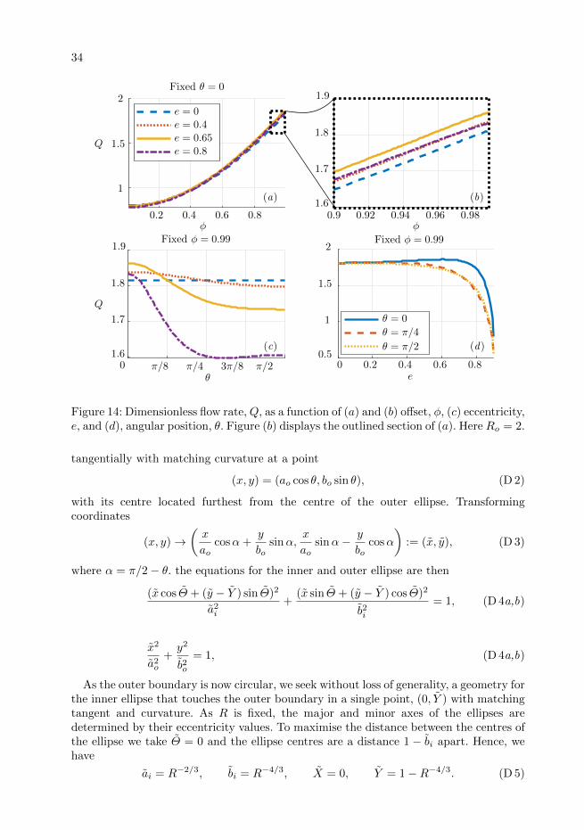
34

0.4 0.6 0.8

1

1.5

2

e = 0.4e = 0.65e = 0.8

1.9

1.8

1.7

1.60.9 0.92 0.94 0.96 0.98

Fixed θ = 0

Q

φ

Q

φ

θ

Fixed φ = 0.99 Fixed φ = 0.99

e

0.2

e = 0

(a) (b)

1.9

1.8

1.7

1.6(c)

2

1.5

1

0.50 π/8 π/4 3π/8 π/2 0 0.2 0.4 0.6 0.8

(d)

θ = 0

θ = π/4

θ = π/2

Figure 14: Dimensionless flow rate,Q, as a function of (a) and (b) offset, φ, (c) eccentricity,e, and (d), angular position, θ. Figure (b) displays the outlined section of (a). Here Ro = 2.

tangentially with matching curvature at a point

(x, y) = (ao cos θ, bo sin θ), (D 2)

with its centre located furthest from the centre of the outer ellipse. Transformingcoordinates

(x, y)→(x

aocosα+

y

bosinα,

x

aosinα− y

bocosα

):= (x, y), (D 3)

where α = π/2− θ. the equations for the inner and outer ellipse are then

(x cos Θ + (y − Y ) sin Θ)2

a2i+

(x sin Θ + (y − Y ) cos Θ)2

b2i= 1, (D 4a,b)

x2

a2o+y2

b2o= 1, (D 4a,b)

As the outer boundary is now circular, we seek without loss of generality, a geometry forthe inner ellipse that touches the outer boundary in a single point, (0, Y ) with matchingtangent and curvature. As R is fixed, the major and minor axes of the ellipses aredetermined by their eccentricity values. To maximise the distance between the centres ofthe ellipse we take Θ = 0 and the ellipse centres are a distance 1 − bi apart. Hence, wehave

ai = R−2/3, bi = R−4/3, X = 0, Y = 1−R−4/3. (D 5)

35

Q = 2.59 Q = 2.44 Q = 2.14 Q = 1.99

Q = 2.50 Q = 2.53 Q = 2.61 Q = 2.37

0.6

0.3

0

−2.58 2.58 2.58 2.58 2.58−2.58 −2.58 −2.58

2−2 −2.05 2.05 2.24−2.24 −3.03 3.03

eo = 0.8Vary θ

θ = 0Vary eo

(a) θ = 0 (b) θ = π/6 (c) θ = π/3 (d) θ = π/2

(e) eo = 0 (f) eo = 0.3 (g) eo = 0.6 (h) eo = 0.9

Figure 15: Dimensionless velocity colourmaps with dimensionless flow rates, Q. Axes arein (x, y) coordinates and these vary with eccentricity as the available space for fluid flowis constant. Plots (a)-(d) show the effect of the position of the inner ellipse, θ, and plots(e)-(h) show the effect of the outer ellipse eccentricity, eo. Given θ and eo, we solve forX, Y , and Θ, so that the ellipses touch at a single point with matching tangent andcurvature.

We can therefore determine the position and orientation angle of the initial ellipse byreversing the transformation (D 3). Some velocity colourmaps are shown in Figure 15.The values for θ and eo in Figures 15a-h correspond to those in Figures 5e-l, respectively.This comparison shows that Q is larger for ei, Θ that match the curvature of the outerellipse (Figure 15), compared to ei = eo and Θ = 0 (Figure 5).

Appendix E. Optimisation constraints (Section 3.4)

From equations (3.8), we have that the equations of the outer and inner ellipses canbe written respectively as

xTAx = 0, xTBx = 0,

where x = (x, y, 1)T and A and B are symmetric matrices of coefficients, functions ofthe components of g (equation (3.6)). The intersections of two conics can be determinedby considering their pencil, λA+B (Casey 1893). Conditions to determine the relativeposition of two ellipses were derived by Etayo & Gonzalez-Vega (2006), which we canthen write in terms of the components of g. The characteristic polynomial of the pencil(once turned monic) is

f(λ) = λ3 + aλ2 + bλ+ c. (E 1)

36

In order for the inner ellipse to be fully enclosed in the outer ellipse the followingconditions must hold

a > 0, −3b+ a2 > 0, 3ac+ ba2 − 4b2 > 0, (E 2a,b,c)

−27c2 + 18cab+ a2b2 − 4a3c− 4b3 > 0, (E 2d)

along with conditions

n22det(N) > 0, det(N11) > 0, (E 3a,b)

where N = vA + B = (nij) and N11 is the minor of N (Etayo & Gonzalez-Vega 2006).Equations (E 2) and (E 3) provide a set of six nonlinear constraints on g. Thus, theoptimisation problem can be formulated as equation (3.8)

ming−Q, s.t. c > 0, (E 4)

where

c =

a

−3b+ a2

3ac+ ba2 − 4b2

−27c2 + 18cab+ a2b2 − 4a3c− 4b3

n22det(N)

det(N11)

. (E 5)

Appendix F. Additional results (Sections 4.1 and 4.2)

Sections 4.1 and 4.2 explore Stokes resistance to rod motion for a circular rod and acircular outer cylinder, respectively. Although we fix the eccentricity of either the rodor bounding cylinder in each section, the parameter space remains vast and comprises:the position of the rod, the eccentricity of the rod or outer cylinder, and the six Stokescoefficients. We have highlighted key results in Figures 8 and 9 and provide plots ofadditional results (which we refer to in the main text) in this Appendix for completeness.

F.1. Section 4.1

We plot Kxx as a function of relative offset (which varies from 0 when the rod isconcentric to 1 when the rod touches the boundary∗) in Figure 16a for eo = 0, eo = 0.6,and eo = 0.8 (lines i, ii, and iii, respectively). For each offset value, Kxx increases witheo, though it should be noted that when plotting Kxx as a function of absolute offsetX, a crossing of the curves is observed (see inset plot in Figure 16a); this is due to thefact that with higher eccentricity, there is a larger absolute distance to the edge. In allcases we compute the lift force Kxy = 0 (to within numerical error), which is expectedby the symmetry of the domain. We next consider the coupling coefficients Cx and Cy.For concentric circular cylinders, there is no coupling between translation and rotation,i.e., Cx = Cy = 0 (see Section 1.2). However, coupling does occur when there is anoffset; e.g. when the rod is rotating and positioned away from the centre of the outercylinder, the viscous fluid provides both an opposing torque and a force orthogonal tothe minimal spacing. The force parallel to the minimal spacing in this scenario is zero

∗For all eo values shown, the rod can fit tangent to the vertex, so X/(ao−1) = 1 is achievable.

37

ii

i

iii

0.80.60.40.20

Kxx

X/(ao − 1)

0

1000

2000

3000

0 0.80.4100

400

800

ii

iii

ii

i

iii

i

X

Cy

120

80

40

00 0.2 0.4 0.6 0.8

0

100

200

300

X/(ao − 1)

0.5 1 1.5X

Slezkin(1955)

0

ii

i

ii

i

iiiiii(a)

Figure 16: Results for Ro = 2. (a) Rod of unit radius centred at (X, 0), translating withunit velocity in the x-direction. Kxx is plotted both as a function of relative offset andof X (inset) for three values of eo: (i) eo = 0 (ii) eo = 0.6 and (iii) eo = 0.8.(b) Rod centred at (X, 0), rotating with unit velocity in the clockwise direction for (i)eo = 0, (ii) eo = 0.6, and (iii) eo = 0.8. The solution for eo = 0 is compared againstthe analytical solution – Slezkin (1955), dashed black line. The main plot is function ofrelative offset, and inset is a function of X.

(Slezkin 1955). We now explore how these results extend for a circular rod in an outerelliptical cylinder. We determine that, as with a circular outer cylinder, if the rod is offsetin the x-direction, the coupling coefficient Cx = 0, while Cy 6= 0 for all eo with X 6= 0. InFigure 16b we plot Cy as a function of relative offset for eo = 0, eo = 0.6, and eo = 0.8(lines i, ii, and iii, respectively). As observed by the crossing of the curves, for smallrelative offset the coupling is highest for the circular rod, while for large offset the mosteccentric rod has the largest coupling coefficient. That is, as the inner rod approachesthe edge of the domain, the fluid couples rotation to vertical force (and likewise verticalvelocity to torque) more strongly for increased eccentricity. Again, the picture appearsdifferently when plotted against absolute offset, since a greater total distance is availablewith increased eccentricity: for each absolute distance X, Cy decreases with eccentricity(plotted in the inset).

F.2. Section 4.2

Figure 17a plots Azz as a function of absolute offset, 1.45 6 X 6 1.8, for ei = 0.7,continuing the plot on Figure 9a for larger values of X. We observe the same line crossingbehaviour noted for ei = 0.9 in Figure 9a.

Figure 17b plots Kxx (dotted), Kyy (dashed), and Kmin (solid) for ellipses of eccen-tricities ei = 0, ei = 0.7, and ei = 0.9, all oriented at angle Θ = π/2. We see that overthis range of offset values (0 6 X 6 1.45), Kmin = Kyy, and kmin = ey.

Figures 17c-h show either coupling or lift coefficients for ei = 0.7 (left column) andei = 0.9 (right column) as functions of absolute offset, X. The dashed black lines aredifferent Θ values, ranging from Θ = 0 to Θ = π/2 in steps of π/40. In each plot, the Θvalue that maximises the force coefficient (over the majority of the X range) is indicatedby a solid red line. Schematics indicate orientation for the minimal and maximal lines.

The coupling between rotation and translation in the x-direction is shown in Figures17c-d. We see that for Θ = 0 and Θ = π/2, Cx = 0. Over the majority of the offsetvalues, Cx is maximal when Θ = π/4. However, for ei = 0.9, there is a region close tothe outer boundary, where smaller offset angles provide a higher coupling force.

The coupling between rotation and translation in the y-direction is shown in in Figure

38

17e and Figure 17f. For both ei = 0.7 and ei = 0.9, Cy increases monotonically with Θfrom Θ = 0 to Θ = π/2 over the full range of offset values.

The lift force, Kxy is plotted in Figure 17g and Figure 17h. This is zero for Θ = 0 andΘ = π/2 and maximal (over the majority of the offset values) for Θ = π/4. However, forei = 0.9, as with Cx, there is a region close to the boundary, where crossing of the linesoccurs.

Appendix G. Absolute vs. relative distance from the wall

In Figure 11, the closest distance to the wall at each value of angular position θ istaken as φ = 0.99, with φ and θ defined as in Figure 4: φ = 0 corresponds to the rodpositioned in the centre of the outer cylinder (X = Y = 0) and φ = 1 denotes the rodtouching the cylinder wall. For each value of (φ, θ), the position of the rod is

X = φ(ro − ri) cos θ, Y = φ(ro − ri) sin θ, (G 1)

where ro and ri are the effective radii of the inner and outer ellipses at an angle θ, asdefined in equation (3.3). Because the radius of the inner and outer ellipses vary withangular position θ, φ provides a ‘relative’ position for the rod; i.e., the absolute distancebetween the edge of the rod and the cylinder is different for constant φ at each value ofθ. In Figure 18 we test the sensitivity to the fixed distance from the wall of the observedcorrespondence between positions of highest minimum resistance and maximum axialflux in Figure 11 (where ei = eo = 0.7, Θ = 0). Positions for the rod with an absolutedistance, δ, are

X = (ro − ri − δ) cos θ, Y = (ro − ri − δ) sin θ. (G 2)

We plot, as the solid lines in Figures 18a,c, Q and Kmin, respectively, for fixed values ofφ = 0.9, 0.925, 0.95, 0.99 (increasing φ correlates with decreasing distance between therod and the cylinder wall). We see that the position that provides both maximum fluxand highest minimum resistance is at θ = 0 for all values of φ. We compare this with fluxand resistance when the rod is positioned at an absolute distance from the edge of thecylinder, δ. In Figures 18b,d, we again plot Q and Kmin, respectively, but now for fixedδ = 0.1, 0.05, 0.025, 0.01 (dashed lines). We see that the qualitative nature of the curvesis unchanged, and that again, the position of both maximum flux and highest minimumresistance is at θ = 0 for all values of δ.

39

0 0.4 0.8 1.2 1.410.60.2X

K

30

50

70

90

110

Azz

Kxx

Kyy

Kmin

20

30

40

50

60

1.45 1.8X

(a) (b)

0 0.4 0.8 1.2 1.410.60.2X

−40

Cy

0

20

−20

Θ

Kxy

20

30

0 0.4 0.8 1.2 1.410.60.2X

0 0.4 0.8 1.2 1.410.60.2X

Cx

0

20

40

60

0

3

6

9

Cx

0

3

6

9

0 0.4 0.8 1.2 1.410.60.2X

Cy

0 0.4 0.8 1.2 1.410.60.2X

Θ

(c) (d)

(e) (f )

0 0.4 0.8 1.2 1.410.60.2X

0

4

8

12

Kxy

0

10

(h)(g)

Figure 17: Figure (a) shows Azz as a function of offset for ei = 0.7 oriented at Θ = 0,Θ = π/4, and Θ = π/2. Offset, X ∈ [1.45, 1.8] (a continuation from Figure 9a). Figure(b) shows Kmin for ei = 0, ei = 0.7, and ei = 0.9 all oriented at Θ = π/2. Figures (c)-(h)show coupling and lift force coefficients for ei = 0.7 (left column) and ei = 0.9 (rightcolumn). Orientation angles vary between Θ = 0 and Θ = π/2 in steps of π/40.

40

0 π/4 π/2

100

120

140

θ

Q(a) Relative distances, Q

φ = 0.9φ = 0.925φ = 0.95φ = 0.99

0 π/4 π/2

100

120

140

θ

Q

(b) Absolute distances, Q

δ = 0.1δ = 0.05δ = 0.025δ = 0.01

0 π/4 π/2

200

400

600

800

θ

Kmin

(c) Relative distances, Kmin

0 π/4 π/2

200

400

600

800

θ

Kmin

(d) Absolute distances, Kmin

Figure 18: Plots of Q (a,b) and Kmin (c,d) as functions of angular position θ (see Figure4) for different offset values from the wall. Figures (a) and (c) with solid lines showrelative distances, denoted with φ (Figure 4) and absolute distances, δ.