The Effect of Teachers’ Unions on Student Achievement:

Evidence from Wisconsin’s Act 10

E. Jason Baron∗

March 3, 2018

Abstract

This study examines the short-run impact of a weakening of teachers’ unions on

student achievement. In 2011, Wisconsin enacted the Budget Repair Bill, or Act 10,

which significantly limited the power of teachers’ unions in the state by restricting

their fundraising abilities and limiting the scope of collective bargaining. Exploiting

plausibly exogenous variation in the timing of exposure to Act 10 due to differences

in the expiration dates of pre-existing collective bargaining agreements across school

districts, I find that the law reduced average test scores on the state’s standardized

exam by approximately 20% of a standard deviation. Results from quantile regressions

indicate that this effect was largely driven by declines in the lower half of the student

achievement distribution. Lastly, the study explores plausible mechanisms behind the

observed decline in achievement, and presents evidence that the law led to a significant

increase in teacher turnover and a large reduction in teacher salaries.

∗Department of Economics, Florida State University. E-mail: ejb15c@my.fsu.edu

1 Introduction

Throughout the second half of the twentieth century, the United States experienced a steady

increase in public sector unionism (Freeman, 1988). This phenomenon started in the 1960s

when various states passed favorable collective bargaining legislation for government work-

ers (Frandsen, 2016). In an effort to address state budget deficits resulting from the Great

Recession, however, policymakers throughout the country have recently implemented legis-

lation that limits the influence of public sector unions. The architects of these laws argue

that reducing union power allows states to decrease the salaries and pensions of government

workers, which can generate significant cost savings (Freeman and Han, 2012). Wisconsin’s

2011 Budget Repair Bill (or Act 10), a well-documented example of such legislation, severely

reduced the influence of public sector unions in Wisconsin by limiting the scope of union

negotiations and restricting their fundraising abilities.

Roughly half of Wisconsin’s public sector employees belonged to a union prior to 2011,

well above the national average of 30%. Figure 1 shows the dramatic decline in public

sector union membership in Wisconsin following the enactment of Act 10 in 2011. While

the national average stayed constant at 30%, Wisconsin’s public sector union membership

plummeted from 50% in 2011 to 37% in 2012, and continued to decrease in the following

years to roughly 22% in 2016. This effect was largely driven by declines in the membership

of teachers’ unions in the state. Reports from the local press indicate that the state’s

largest teachers’ union, the Wisconsin Education Association Council (WEAC), experienced

a decline in membership of more than 50% (or 60,000 members) from 2011 to 2015.1

This paper seeks to identify the short-run impact of a weakening of teachers’ unions

on student achievement by exploiting a natural experiment that took place in Wisconsin

following the enactment of Act 10. While the bill was signed into law on June 29, 2011, Act

10’s provisions became effective only after the expiration of pre-existing collective bargaining

agreements (CBAs). Therefore, public school districts whose labor contracts expired in 2011

were immediately affected by the law during the 2011-12 academic year, while districts that

had pre-existing contracts with longer terms were insulated from the provisions in Act 10

until their contracts expired. I exploit these plausibly exogenous differences in the timing of

exposure to Act 10 in an event study framework to estimate the impact of limiting union

power on student achievement.

The net effect of a weakening of teachers’ unions on student achievement is unclear a

1See, for example: Beck (2015), WEAC Turns to Local Focus After Massive Membership Loss, WisconsinState Journal. Accessed at: http://host.madison.com/wsj/ (August 11, 2017).

1

priori, as both economic theory and previous literature yield ambiguous predictions of the di-

rection of this effect. Teachers’ unions influence public education in the U.S. mainly through

the collective bargaining process.2 They seek to maximize the utility of their members by

bargaining with local school boards for higher wages and benefits, job security, and more

favorable working conditions such as smaller class sizes (Lovenheim, 2009). Additionally,

unions often bargain for teacher compensation schemes that are based solely on seniority

and educational attainment, rather than on student outcomes, and often protect teachers

with longer tenure from layoffs or less desirable school assignments (Strunk et al., 2017; West

and Mykerezi, 2011).

On the one hand, if the incentives created by the union compensation structure reduce the

returns to higher effort and limit the capacity of school administrators to attract young, high-

quality teachers through higher pay, a weakening of teachers’ unions may benefit students

(Figlio, 2002). Student achievement may also increase following a decline in union power

if teachers’ unions reduce teacher effort by protecting the job security of low-productivity

teachers (Lovenheim and Willen, 2016). Union influence over school boards may also lead to

suboptimal budgets for students (Hoxby, 1996). Given a fixed district budget, unions may

force school districts to distribute resources toward teacher pay and away from expenditures

that could otherwise increase student achievement more efficiently. Therefore, a weakening

of unions may help administrators redesign school budgets in a way that improves students’

outcomes.

On the other hand, limiting the influence of teachers’ unions may decrease student

achievement if unions insulate teachers from school administrators’ abuses such as politicized

teacher evaluations and layoff procedures (Freeman and Medoff, 1984). Such protections can

increase work morale, a necessary condition for teachers to exert high effort under incomplete

contracts (Kube et al., 2013). A reduction in teacher compensation, which has been shown

to occur following a weakening of teachers’ unions, may further exacerbate this decline in

morale (Litten, 2016). Lastly, CBAs that reward local seniority may provide incentives for

teachers to remain in the same school district throughout their careers. A decline in union

power may lead to the removal of these incentives and a subsequent increase in teacher

turnover, which has been shown to have disruptive, negative effects on student achievement,

at least in the short run (Ronfeldt et al., 2013).

The net effect of deunionization on student achievement depends on which of the above

2While teachers’ unions can also influence public education through their involvement in the politicalarena, their main role is that of bargaining agents for public school teachers (Cowen and Strunk, 2015).

2

mechanisms dominates. Given the relatively few efforts to limit the influence of public

sector unions prior to 2011, however, the existing empirical literature has not yet reached a

consensus regarding the direction of this effect. For instance, while Hoxby (1996) concludes

that teacher unionization increases high school dropout rates, in a later study Lovenheim

(2009) finds no evidence of this effect. More recently, Lovenheim and Willen (2016) find

that laws requiring school districts to engage in collective bargaining with teachers’ unions

negatively affect the long-run labor market outcomes of male students. Furthermore, these

previous studies have focused on episodes of unionization during the 1960s, and whether the

effects of unionization on student achievement are symmetric to those from deunionization

remains an open empirical question.

In general, I find that average student achievement in Wisconsin high schools decreased

as a result of the union reform. Specifically, the reduction in union power associated with Act

10 reduced composite scores on the state’s standardized exam, the Wisconsin Knowledge and

Concepts Examination (WKCE), by roughly 20% of a standard deviation. This effect was

primarily driven by decreases in the mathematics and science portions of the test. Scores in

these subjects decreased by approximately 30% of a standard deviation as a result of the law.

To understand the economic significance of these effects, one can compare their magnitude

with that from the effect of a reduction in class size of eight students, which has been shown

to increase student achievement by up to 60% of a standard deviation (Angrist and Lavy,

1999; Finn and Achilles, 1990).

Quantile regression techniques reveal substantial heterogeneity in the effects of Act 10

throughout the test score distribution. Particularly, the results indicate that the average

reduction in test scores was largely driven by declines in the lower half of the conditional

WKCE distribution. I find that Act 10 reduced both the median of the test score distribution

and every decile below it. Declines were largest for the lowest deciles of the distribution.

For instance, I find that Act 10 reduced the 10th percentile by roughly 50% of a standard

deviation. However, I find no clear evidence that the law had any impact on deciles in the

upper half of the distribution.

Given that quantile regression estimates reveal effects of the law on the test score dis-

tribution, and not on specific schools, I complement quantile regression techniques with a

subgroup analysis. Results from this exercise indicate that the observed reduction in average

test scores was largely driven by declines in student achievement at initially low-performing

schools.

Finally, I explore plausible mechanisms that may have contributed to the observed decline

3

in student achievement. While many factors including individual characteristics, family

environment, and school inputs such as class size have been shown to influence student

achievement, teacher quality is believed to be the most important school-related input in

the education production function (Rivkin et al., 2005; Rockoff, 2004; Angrist and Lavy,

1999). Given the importance of teachers in the production of student achievement, I begin

by examining how Act 10 impacted Wisconsin’s teacher workforce.

I first present evidence that the law led to a significant increase in the share of inter-

district teacher transfers. I argue that disruptive effects from this unexpected increase in

teacher turnover may be one of the channels through which Act 10 hindered student achieve-

ment. Specifically, Atteberry et al. (2017) and Ronfeldt et al. (2013) argue that, through

a destruction of organizational knowledge, increased costs allocated to the recruiting, hir-

ing, and training of new teachers, and a reduction in the productivity of staying teachers

due to increased responsibilities for mentoring new teachers, turnover can decrease student

achievement.

Second, consistent with the findings of Litten (2016), I find that the law decreased teacher

salaries by roughly 4%. The effect of the decline in salaries on student achievement is

ambiguous a priori. If districts used this additional income to increase expenditures in areas

that more directly benefit students, achievement may increase (Hoxby, 1996). On the other

hand, declines in teacher salaries may decrease work morale and productivity, which may

hinder student achievement (Kube et al., 2013). Using district-level expenditure data, I test

for evidence of a budgetary shift as a result of Act 10. While I present clear evidence of a

reduction in teacher salaries, I find no evidence that the law had an effect on other district-

level expenditures that could more directly impact student achievement. These findings

suggest that the decline in teacher salaries may be another channel through which Act 10

decreased student achievement.

Importantly, since the WKCE was changed in the 2014-15 academic year, I observe (at

most) three years of student outcomes following exposure to Act 10. Thus, the identification

strategy is structured so that the estimated treatment effects are immediate to the decline in

unionization. The findings presented in this study should therefore be interpreted as purely

short-run and likely as a transitional effect from an old steady state to a new equilibrium.

While I provide evidence that Act 10 had negative, disruptive effects on student achievement,

I leave it to future research to fully characterize Wisconsin’s post-Act 10 long-run equilibrium.

Nevertheless, declines in test scores, even in the short run, could have lasting effects on

students. For instance, Chetty et al. (2014) show that teachers’ impacts on student test

4

scores are correlated with students’ long-term outcomes such as teenage pregnancy, college

attendance, and earnings.

My paper makes two main contributions to the literature. First, this study adds to

the extensive, multidisciplinary literature that attempts to identify determinants of student

success (Chetty et al., 2014; Dobbie and Fryer Jr, 2014; Rockoff, 2004; Hanushek et al., 2003)

by demonstrating that a weakening of teachers’ unions hinders student achievement. These

findings differ from those of earlier studies that have focused on episodes of unionization

and have found no evidence of a causal link between teachers’ unions and student outcomes

(Lovenheim, 2009). My results suggest that, while episodes of unionization and processes

that limit union power represent related changes in market structure, their effects on student

achievement can differ in meaningful ways, at least in the short run.

A plausible explanation for these differing effects could be the timing of deunionization

events. Unionization during the 1960s was a very slow process since it required an initial

election, as well as the passage of state laws that facilitated collective bargaining (Hoxby,

1996). Conversely, the recent weakening of teachers’ unions has been sudden and unexpected,

which has limited the ability of school districts to enact anticipatory measures. Another ex-

planation could be asymmetric teacher responses to wage changes. Specifically, loss aversion

suggests that a reduction in salaries following deunionization should decrease teacher pro-

ductivity by a greater magnitude than the increase expected from a symmetric wage raise

following unionization (Kube et al., 2013; Kahneman and Tversky, 1979).

This study also adds to the limited, emerging literature examining the effects of recent

deunionization policies on various outcomes. Han (2015) shows that restrictions on col-

lective bargaining for public school teachers in Indiana, Idaho, Tennessee, and Wisconsin

resulted in lower teacher quality, as measured by the proportion of teachers who are clas-

sified as highly qualified.3 Litten (2016) finds that Act 10 decreased teacher compensation

by roughly 8%. Biasi (2018) examines how school districts’ compensation schemes changed

following the passage of Act 10. Given that the law prohibited collective bargaining over

teacher compensation schemes, school districts were granted the freedom to implement new

forms of compensation. Biasi finds that roughly half of school districts retained their old

unionized compensation schemes, while the other half switched to more flexible compensa-

tion, and documents a sorting of high-quality teachers into districts that adopted flexible

pay. Lastly, Roth (2017) finds that Act 10 led to a significant increase in teacher retirements,

3Highly Qualified Teacher (HQT) determination was a provision under the No Child Left Behind Act of2001. To become an HQT, a teacher required full state certification, a bachelor’s degree, and demonstratedcompetency on a state-administered subject area test (Han, 2015).

5

and documents an increase in value added in elementary school grades with a larger share of

retirees. My paper contributes to this literature by examining how deunionization policies

affect student achievement in the short run.

The rest of the study is organized as follows. Section 2 describes the role of teachers’

unions in Wisconsin before Act 10, as well as the various provisions of the law. Section 3

summarizes the dataset and its sources, while Section 4 describes the empirical approach

and the identifying assumptions. Section 5 presents the results and robustness checks, and

investigates possible mechanisms driving the observed net effect. Section 6 concludes with

policy implications and a potential path for future research.

2 Background

2.1 Unions in Wisconsin Pre-Act 10

In 1959, Wisconsin became the first state to pass a Duty-to-Bargain (DTB) law. This

legislation gave teachers’ unions considerable power. Not only were public school teachers

granted the right to collectively bargain, but the law also required school districts to negotiate

in good faith with their local teachers’ union (Lovenheim and Willen, 2016).

Prior to the enactment of DTB legislation, teachers’ unions in Wisconsin served only as

professional and political advocates for teachers, and had no formal bargaining rights. From

the time they were granted the right to bargain, until 2011, teachers’ unions operated under

a relatively favorable regulatory environment. Unions had the ability to collectively bargain

with school boards over working conditions, layoff procedures, pensions, health care benefits,

teachers’ compensation schemes, and other school-related issues (Ford and Ihrke, 2016).

2.2 Wisconsin’s Act 10

On June 29, 2011 Wisconsin enacted the Wisconsin Budget Repair Bill, or Act 10, which

included a number of provisions that diminished the power of teachers’ unions in the state.

First, the law restricted the scope of collective bargaining to negotiations over base wages

for most state employees.4 Second, it limited base wage increases to adjustments at or below

the inflation rate. Third, Act 10 implemented a right-to-work measure which prohibited

unions from deducting dues from paychecks and allowed employees to refuse to pay agency

4Act 10 excluded public safety employees from its provisions.

6

fees while remaining in the bargaining unit. Fourth, the Act restricted the length of CBAs

to one-year periods.

Fifth, the law created a new system of certification elections. Prior to Act 10, once a

collective bargaining unit elected a labor organization as its representative, the organization

remained the unit’s representative unless a petition was supported for a new election to

decertify. Act 10 required an annual certification election for a union to maintain legal

status. If less than a majority of members in the bargaining unit vote to keep the union, the

union is decertified (Freeman and Han, 2012).

Lastly, prior to the enactment of Act 10 state employees paid on average 6% of annual

health insurance premiums, and most paid little or nothing toward their pensions. Act 10

required state employees to contribute 50% of their annual pension payment and at least

12.6% of their average annual health premiums. Thus, when considered simultaneously, it is

clear that the law severely reduced the influence of teachers’ unions in Wisconsin by limiting

the scope of union negotiations, increasing the costs of unionization, and altering the funding

structure of union activity.

2.3 Wisconsin’s Reduction in State Aid

As mentioned previously, Act 10 policy changes took effect upon the expiration of CBAs

in place at the time of the enactment of the law. However, in addition to Act 10, an

additional piece of legislation targeted public school funding during this time. Under the

2011-13 biennial budget known as Act 32, Wisconsin imposed a significant reduction in state

appropriations to school districts. Unlike the provisions under Act 10, all school districts

were impacted by Act 32 in the 2011-12 academic year, regardless of differences in contract

renewal dates. As I discuss below, the timing and target of Act 32 could potentially confound

my estimates of Act 10.

Both Act 10 and Act 32 were crafted to address the state’s looming budget deficit. The

architects of Act 10 explained that its provisions would allow school districts to generate

enough savings to offset the decrease in state aid, which in turn would help the state reduce

its deficit. School districts in Wisconsin derive a large part of their revenue from two main

sources: state aid and property taxes (over 88% in 2014-15). The rest of their revenues come

from federal aid and local revenues such as interest earnings.5 Most state aid is delivered to

school districts as equalization aid, which is designed to distribute relatively more funds to

5See the Wisconsin Legislative Bureau’s State Aid to School Districts, Informational Paper 24 availableat https://dpi.wi.gov/ for a detailed explanation of Wisconsin’s school-finance system.

7

schools with relatively lower property values. Equalization aid is subject to revenue limits,

which restrict the amount of revenue a district can raise from state aid and property taxes.

Act 32 decreased funding for school districts in two ways. First, it reduced equalization

aid by 8.4% in the 2011-12 academic year (relative to the 2010-11 academic year). Second,

Act 32 reduced each district’s revenue limits by 5.5%.6 The reduction in revenue limits

prevented school districts from simply raising school levies to make up for the lost state

aid. While the 5.5% reduction in revenue limits was uniform, equalization aid reductions did

not affect all school districts in the same way due to the complexity of the equalization aid

formula. In Section 4.1, I investigate whether Act 32 differentially impacted schools exposed

to Act 10 in 2011-12 and those grandfathered by the law for at least a year.

3 Data

3.1 Collective Bargaining Agreements

To estimate the effect of Act 10 on student achievement, I combine two primary datasets.7

First, I obtain the start and expiration dates of finalized CBAs between Wisconsin’s public

school districts and their teachers’ unions for the years 2008-09 through 2013-14.8 The vast

majority of CBAs in Wisconsin are two-year contracts which begin and end in odd-numbered

years. Most districts use a two-year union contract to align themselves with the state’s

biennial budget cycle. However, there is no law that requires districts to contract in this

way, and some districts sign longer contracts, contracts that do not follow the state’s budget

cycle, or both. Variation in the timing and length of contracts among school districts led to

differences in the timing of exposure to Act 10, which grandfathered existing agreements.

I use this dataset to identify which districts signed CBAs in periods prior to the enact-

ment of Act 10 that expired immediately before the 2011-12 academic year and were thus

immediately affected by the law (henceforth referred to as “Immediately Treated”), and

which ones signed contracts that expired after 2011-12, either in 2012-13 or 2013-14 (hence-

6See the Wisconsin Association of School Boards’ 2011-13 Budget Summary available at https://www.

wasb.org/ for a detailed description of Act 32.7Private and charter schools are excluded from the analysis since they are subject to different state and

local regulations.8I obtained this dataset from the Wisconsin Education Association Council. While this dataset contained

information on most school districts, I supplemented it with phone interviews, e-mails, and contracts providedto me by a reporter at the Milwaukee Journal Sentinel who had collected a random sample of contracts forhis own purposes.

8

forth referred to as “Grandfathered”).9 I identified fifteen districts (seventeen high schools)

in the latter category. Of these seventeen schools, ten of them had contracts expiring in

2012-13, and the remaining seven had contracts that expired in 2013-14. This is the key

variation in timing that allows me to identify the effect of the law on student achievement.

It is important to note that some teachers’ unions rushed to sign extensions of their CBAs

as soon as they found out about the law. However, after carefully reviewing a subsample

of these extensions and talking with school administrators, it is evident that unions had to

make concessions that mirrored those from Act 10 very closely in order to convince districts

to extend their contracts. This was due to the fact that school boards were aware of the

impending enactment of Act 10, which increased their bargaining power.

I include two types of districts in the Immediately Treated group: those whose contracts

expired in 2011-12 and no extension was signed, and those that agreed to sign an extension

after the law was announced. The fifteen districts in the Grandfathered group are those

that signed an initial contract with an expiration date of 2012-13 or 2013-14, and did so in

a period prior to any announcement of the law. This classification guarantees that schools

in the Grandfathered group did not endogenously sign a longer contract in response to the

impending enactment of the bill.

3.2 Administrative Dataset

Information on each school’s timing of exposure to Act 10 is matched to administrative data

from the Wisconsin Department of Public Instruction (WDPI). The WDPI reports each

public school’s average student achievement scores and student demographics. District-

level expenditures, revenue limits, and equalization aid are also reported. I complement

these school/district-level files with an individual-level dataset published annually by the

WDPI. This dataset contains detailed information on the universe of Wisconsin public school

teachers. It includes covariates such as each teacher’s first and last name, district and school

of employment, birth year, total salary and fringe benefits, and years of teaching experience.

I use the individual-level dataset to compute variables not reported in the school-level

files such as the school’s average teacher experience and compensation (salary + fringe

benefits), as well as each school’s retirement and turnover rates. When computing school-

level averages from the individual-level dataset, I weight teachers by their corresponding

9Pre-existing CBAs of districts in the Immediately Treated group expired on June 30th, 2011. Since Act10 was enacted on June 29th, 2011 these districts were immediately exposed to the law. In contrast, CBAsof districts in the Grandfathered group expired on either June 30th, 2012 or June 30th, 2013. Thus, theseschools were grandfathered by the law for either one or two years.

9

FTE units. Following Roth (2017), the school’s retirement rate is imputed as the attrition

rate for retirement-eligible teachers.10 Thus, the retirement rate for school s in year t is

computed as the fraction of total teachers in year t who are eligible to retire and leave the

sample in year t + 1.11 I compute the teacher turnover rate for school s in year t as the

proportion of teachers in the school who transferred from a school outside the district at

time t. This definition is similar to the one used by Ronfeldt et al. (2013).

I use each school’s average test score (by subject) on the state’s standardized test, the

WKCE, as the measure of student achievement.12 Federal law requires an annual review of

student academic progress. In Wisconsin, students demonstrate their progress in five areas

(reading, language arts, mathematics, science, and social studies) through their participation

in the WKCE. The test is administered every fall to students in grades four, eight, and ten.

While WKCE performance data exist for all three grades, I conduct the analysis at the high

school level since a significant amount of data is missing for elementary and middle schools

due to confidentiality reasons. The WDPI protects student privacy by suppressing records

of student groups that could be potentially identified through publicly available data. Due

to smaller school sizes, I found this to be a larger issue in elementary and middle schools.

The WKCE is used as the measure of student achievement for three reasons. First,

Chetty et al. (2014) show that impacts on student test scores are correlated with students’

long-term outcomes such as teenage pregnancy, college attendance, and earnings. Second,

studies that use measures such as high school dropout rates or ACT and SAT scores can

only capture the achievement of students at the tails of the ability distribution. Analyses

of dropout rates (Lovenheim, 2009; Hoxby, 1996) are focused on students at the lower end,

while those using SAT and ACT scores (Kleiner and Petree, 1988) focus on students at the

upper end. Since nearly every public high school student is required to participate in the

WKCE, this assessment provides a measure of achievement throughout the entire ability

distribution.13 Third, although the exam was changed in 2014-15, year-to-year comparisons

10Wisconsin public school teachers are eligible for early retirement at age 55. As Roth notes, a weaknessof this definition is that, since the sample is restricted to public school regular educators, a person thattransitions into either a private school or an administrative role is classified as having exited the teachingprofession.

11Roth includes only retirement-eligible teachers in the denominator. Given that my analysis is at thehigh school level, there are some schools with no retirement-eligible teachers at time t. Therefore, using thisdefinition generates multiple missing values. To overcome this, I use the total number of teachers in school sat time t in the denominator. The results using Roth’s definition instead tell a similar story and are availableupon request.

12See the WSAS Administrator’s Interpretive Guide available at https://dpi.wi.gov/ for a thoroughdescription of the exam.

13If the Individualized Education Program (IEP) team determines that a student with significant cognitive

10

are valid for 2005-06 through 2013-14. This allows me to examine outcomes in every school

in my sample for at least one year after initial exposure to Act 10.

3.3 Final Sample

In my main analysis, I drop the districts of Milwaukee Public Schools and Madison Metropoli-

tan Area from the sample. Milwaukee/Madison enroll a significantly larger share of students

than the rest of school districts in Wisconsin. Furthermore, high schools in these two dis-

tricts are substantially different from those in other Wisconsin school districts, which are

largely located in rural or suburban areas.14

Columns 1 and 2 of Table 1 report the pre-2011 means and standard deviations (in

parentheses) of various observables separately for high schools in the Milwaukee/Madison

districts and high schools in the rest of districts in my sample. Column 3 reports the point

estimates and robust standard errors (in parentheses) of tests for equality of means.

Overall, high schools in these two groups are significantly different across pre-2011 WKCE

scores, student demographics, teacher characteristics, and finances. As an example, high

schools in Milwaukee/Madison enroll approximately 790 students more, on average, than

high schools in the remaining school districts. Furthermore, the average share of minorities

in high schools in Milwaukee/Madison is roughly 72%, compared to only 10% for high schools

in the remaining districts.

One may be concerned with the robustness of this study’s main findings to the exclusion

of Milwaukee/Madison from the sample, particularly since Milwaukee is a notable example

of a grandfathered school district. Thus, in Appendix A I show that including these two

districts in the analysis does not qualitatively change my results.

The final sample contains a balanced panel of 380 high schools for the years 2005-06

through 2013-14. As mentioned above, while there are 410 regular public high schools in

Wisconsin, outcome data is missing for some schools due to confidentiality reasons. Nev-

ertheless, the schools included in the final sample enroll roughly 97% of all students in

Wisconsin public high schools.15 Of the 380 high schools in my sample, 363 are classified

as immediately treated and 17 as grandfathered by Act 10. In the next section, I examine

empirical differences between schools in these two groups.

disabilities is unable to participate in the WKCE, even with accommodations, the student instead participatesin the Wisconsin Alternate Assessment for Students with Disabilities (WAA-SwD). Source: WDPI.

14I thank an anonymous referee for this observation.15Author’s calculation from high school enrollment data. This exercise excludes Milwaukee/Madison from

the denominator.

11

4 Empirical Strategy

Simply regressing a school’s average student achievement score on a measure of union

strength would likely yield a biased estimate due to either simultaneity or omitted-variable

bias. As an example, teachers’ unions may be more powerful in school districts where teach-

ers are treated particularly poorly. Since teacher morale may be correlated with both union

influence and student achievement, making causal claims regarding the effect of teachers’

unions on student outcomes is difficult. To address this issue, the literature has largely

relied on variation in state laws that facilitate collective bargaining for teachers (Lovenheim

and Willen, 2016; Lovenheim, 2009; Hoxby, 1996).

In contrast to these studies, this paper employs a within-state analysis. Specifically, I

exploit a natural experiment that took place in Wisconsin following the enactment of Act

10. Differences in the term lengths of pre-existing CBAs caused some districts to be exposed

to the law in 2011-12, while the remaining districts were unaffected until either the 2012-13

or 2013-14 academic year. To identify the effect of the law on student achievement, I exploit

variation in initial exposure to Act 10 by estimating the following panel regression:

Achievementsdt = γAct10dt + µs + αt +Xsdtβ + εsdt (1)

where s denotes the school, d the district, and t the year. Achievementsdt is the school’s

average WKCE score, by subject, which I standardize within subject using the state’s 2005-

06 WKCE score distribution.16 Act10dt is the independent variable of interest and it is

equal to one if school district d is subject to Act 10 in time t, and zero if it is covered by

a pre-existing CBA. The specification additionally includes both school (µs) and year (αt)

fixed effects. Here, µs controls flexibly for any time invariant school-specific characteristics

such as preferences for student achievement and unionism, while αt controls for any time-

varying shocks that affect all Wisconsin schools in the same way such as changes in the

state’s economic conditions. Finally, Xsdt is a vector of district and school-level covariates

such as student demographics and sources of revenue.

16Specifically, I perform a z-score transformation for each WKCE subject using the mean and the standarddeviation of the 2005-06 test score distribution. Results are robust to standardizing using any other pre-2011year in the sample.

12

4.1 Identifying Assumptions

The identifying assumptions of this model are that (1) (conditional on fixed effects and

covariates) the timing of exposure to Act 10 is exogenous and that (2) student achievement

in immediately treated schools would have evolved in the same way as schools grandfathered

by Act 10, were it not for the union reform. Under these assumptions, γ will represent

the Average Treatment Effect (ATE) of weaker union power, through Act 10, on student

achievement.

The first assumption appears to be reasonable. School districts that signed longer con-

tracts in periods prior to Act 10 did so because difficult negotiations with their teachers’

unions led to delayed contracts in the past. In order to avoid the costs of negotiating again

soon after the delayed contract was signed, there was a mutual agreement to simply sign a

longer contract. An immediate concern may be that difficult negotiations were the result of

some districts “valuing” education differently than others. However, it is important to note

that as long as differences between these districts are (approximately) time invariant, the

inclusion of school fixed effects is likely to eliminate most of this variation.

I investigate the first assumption further by checking for balance in the means of pre-

2011 observable characteristics across schools in the Immediately Treated and Grandfathered

groups. If the decision to sign a longer contract in a period prior to Act 10 is related to school

quality, test scores should differ across the groups prior to the enactment of the law. Columns

1 and 2 of Table 2 report the means and standard deviations (in parentheses) by school type

and averaged in the four years preceding the enactment of Act 10 (2007-08 through 2010-11).

Column 3 reports the point estimates and robust standard errors (in parentheses) of tests

for equality of means. Overall, immediately treated and grandfathered schools had similar

WKCE scores, student demographics, teacher characteristics, and finances before Act 10

was enacted. Given the similarity between the groups prior to Act 10, it is plausible that

contract expiration dates were exogenously determined.

Two necessary conditions must be met for the second identifying assumption to hold:

immediately treated and grandfathered schools are on parallel trends prior to Act 10 expo-

sure, and there are no differential shocks (other than the timing effects of Act 10) in the

treatment period. In the next section, I show using an event study framework that the first

necessary condition is met. I focus on the second necessary condition here. As mentioned

in Section 2, Act 32 decreased school districts’ equalization aid and revenue limits in the

2011-12 academic year. If Act 32 impacted schools in the Immediately Treated and Grand-

fathered groups differently, the effects of Act 32 and Act 10 may be confounded. To test

13

this, I estimate the following equation:

Ysdt = ζ(Postt)+ω(ImmediatelyTreatedsd)+ψ(Postt×ImmediatelyTreatedsd)+υsdt (2)

where Ysdt is either revenue limits or equalization aid, Postt is a dummy variable that is

equal to one in 2011-12 and every subsequent year, ImmediatelyTreatedsd is a dummy

variable that is equal to one if the school belongs to the Immediately Treated group, and

Postt × ImmediatelyTreatedsd is an interaction term between the two.

The parameter of interest is ψ, the differential effect of Act 32 on schools in the Immedi-

ately Treated and Grandfathered groups. If Act 32 affected the groups differently, estimates

of ψ should be statistically significant. The estimated coefficients of Equation 2 are shown in

Table 3. I am unable to reject the hypothesis that Act 32 affected schools in the Immediately

Treated and Grandfathered groups in a similar manner. This finding, the inclusion of year

fixed effects, and the fact that Act 32 affected all districts in the same year should allow me

to identify the effects of Act 10 using Equation 1, and without potential confounding effects

from Act 32. In the next section I additionally show that the estimates of γ are robust to

the inclusion and exclusion of school-finance covariates. Altogether, the evidence provided

in this section suggests the identifying assumptions of the baseline model are likely to hold.

5 Results

The baseline results are shown in Table 4. The table presents estimates of γ for each WKCE

subject along with standard errors in parentheses and clustered at the district level.17 It

shows the robustness of the estimates across five different specifications. First, I weight

specifications in columns 2-5 by the school’s (logged) total enrollment.18 I do this to assess

the robustness of the estimates once I account for the large heterogeneity in size across

Wisconsin high schools.

Second, to obtain a more precise estimate of the treatment effect I add to the regres-

sion school demographics and financial variables as controls in columns 3-4. Inclusion of

these covariates serves as an additional robustness check; estimates of the treatment effect

should not be sensitive to the inclusion of additional covariates if contract timing was in-

deed exogenously determined. As a final robustness check, in column 5 I add school-specific

17The results are robust to clustering at the school level, or two-way clustering at the school and districtlevel.

18The results are robust if I instead weight the regressions by the school’s total enrollment.

14

linear trends. While constrained to be linear, the inclusion of school-specific trends allows

immediately treated schools to follow different trends from grandfathered schools prior to

the enactment of Act 10. Robustness of the estimated treatment effect to the inclusion of

school-specific trends would further indicate that the identifying assumptions of the model

may be satisfied.

Overall, the estimates are robust to the specification choice and indicate that Act 10

reduced WKCE composite scores by approximately 20% of a standard deviation. This

effect is primarily driven by decreases of up to 32% of a standard deviation in science and

mathematics, and a decline of roughly 23% in language arts. The magnitude of these results

can be more easily interpreted by comparing it with the effect of a reduction in class size

of eight students, which has been shown to increase student achievement by up to 60%

of a standard deviation (Angrist and Lavy, 1999; Finn and Achilles, 1990). Even though

all coefficient estimates are negative for social studies and reading, they are statistically

insignificant. This may suggest that science and mathematics are most responsive to school

inputs.

5.1 Event Study Specification

The estimates of γ shown in Table 4 represent a weighted average of union reform effects by

year. Thus, they provide no information about the magnitude of the effects of the law over

time. To uncover these effects, I estimate the following event study specification:

Achievementsdt =∑j 6=−1

γjD(t− year = j) + µs + αt +XsdtΘ + εsdt (3)

where the term year refers to the academic year in which school s is treated by the law - the

academic year following the expiration of the school’s CBA, and the expression D(t−year =

j) is a dummy variable that equals one when school s is j years from treatment. I omit the

year prior to treatment in order to make all estimates relative to this year.

I include six leads and two lags of the treatment effect so that γj represents the coeffi-

cient on the jth lead or lag. This specification is attractive for two main reasons. First, an

alternative test for identifying assumption (2) is that γj = 0 for all j < 0. Rather than con-

trolling for differential pre-law trends across immediately treated and grandfathered schools,

this specification allows me to directly test for the existence of such differentials without

imposing a linear structure on the time pattern of the effects of the law (Lovenheim, 2009).

Second, this model allows for γj, j > 0 to differ by year. This allows me to estimate whether

15

the treatment effect is decreasing or increasing in magnitude over time.

Results from the estimation of Equation 3 are shown in Table 5. The table presents

the estimates and standard errors of the effects of the law leading to and following treat-

ment. A visual representation of the estimates, along with 95% confidence intervals is also

provided in Figure 2. Prior to treatment, estimates across all subjects are individually and

jointly insignificant at the 5% level. This result offers evidence that immediately treated and

grandfathered schools had a similar evolution in the outcome variable prior to treatment.

Following Act 10 exposure, WKCE composite scores decrease by approximately 22% of a

standard deviation and continue to decrease in the subsequent year (roughly by 32% of a

standard deviation). As in Table 4, this effect is primarily driven by decreases in the science,

mathematics, and language arts portions of the test.

5.2 Distributional Effects

This study has provided empirical evidence that Wisconsin’s union reform decreased average

student achievement in the short run. While this average effect is of great interest, an exam-

ination of the effects of the law at different parts of the conditional distribution of student

achievement can have important policy implications. As an example, policy responses and

societal costs associated with the effects of the law may differ depending on which part of

the distribution was affected the most, and simply uncovering the average effect does not

address this question. Furthermore, this exercise may yield important insight into which

possible mechanisms might account for the observed decline in student achievement.

To examine the distributional effects of Act 10, I specify a quantile regression following

the approach outlined in Abrevaya and Dahl (2008). This method resembles Chamberlain’s

Correlated Random Effects (CRE) approach. Unlike the expectation operator, conditional

quantiles are not linear operators. Thus, a fixed effects strategy that eliminates the school

fixed effect µs through differencing techniques is infeasible. Instead, I explicitly control for

unobserved heterogeneity by modeling the school fixed effect using a Mundlak representation.

In a linear panel data model, this approach yields the fixed effects estimator (Wooldridge,

2010). Results from the estimation of this model are presented in Figure 3. The figure

presents point estimates and 95% confidence intervals of the effects of Act 10 at each decile

of the conditional (composite) WKCE distribution. It also presents the OLS estimate (long-

dash) and its confidence interval (short-dash).

As expected, the OLS estimate under the CRE approach is identical to the estimate

obtained using school fixed effects instead, and indicates that Act 10 decreased average

16

WKCE scores by roughly 20% of a standard deviation. However, the figure shows substantial

heterogeneity in the effects of Act 10 throughout the test score distribution. The observed

negative effect of the law on average student achievement is largely driven by declines in the

bottom half of the distribution. Specifically, the figure shows that Act 10 reduced both the

median of the test score distribution and every decile below it. The decline for the lowest

deciles was the largest. For instance, the figure shows that Act 10 reduced the 10th percentile

of the distribution by roughly 50% of a standard deviation. Interestingly, the figure provides

no clear evidence that the law had any impact on deciles in the upper half of the distribution.

One must be cautious when interpreting these results. Quantile estimates reveal effects of

the law on the test score distribution, not on specific schools. The results do not necessarily

imply that schools that were low-performing before Act 10 are now worse off. This can only

be concluded under the assumption that the law was rank-preserving (Angrist and Pischke,

2008). Thus, as an alternative way to explore distributional effects, I perform a subgroup

analysis. Specifically, I segment the data into initially low (those schools in the bottom half

of the pre-Act 10 composite WKCE distribution) and high-performing schools (those in the

upper half), and estimate the event study specification given in Equation 3 separately for

each group.

The results from this estimation are shown in Figure 4.19 I present estimates for composite

scores, as well as for the science and mathematics portions of the exam since these seem to

be the most responsive to school inputs. The figure shows that, in initially low-performing

schools, average scores in science and mathematics decreased by roughly 36% of a standard

deviation immediately following exposure to the law, and continued to decrease during the

following year. However, the figure provides no clear evidence that average test scores in

initially high-performing schools changed as a result of the reform. These results indicate

that the observed negative effect of Act 10 on average student achievement was largely driven

by declines in test scores at initially low-performing schools.

5.3 Mechanisms

The main findings of this study indicate (1) that Act 10 decreased average student achieve-

ment and (2) that this effect was largely driven by declines in test scores at initially low-

performing schools. This section presents a plausible explanation for these results. Although

many factors including individual characteristics, family environment, and school inputs such

as class size can impact student achievement, teacher quality has been shown to be the most

19Point estimates and standard errors (in parentheses) are also presented in Table B.1.

17

important school-related input in the education production function (Rivkin et al., 2005;

Rockoff, 2004; Angrist and Lavy, 1999). Therefore, I first examine how Act 10 impacted

Wisconsin’s teacher workforce.

Figure 5 presents the time series of average teacher compensation, the share of teacher

retirements, and the share of interdistrict teacher transfers in Wisconsin high schools before

and after 2011-12, the academic year in which Act 10 came into effect for the vast majority

of school districts. Changes in the trends of these three variables are notable around the law.

Following the enactment of Act 10, the average share of teachers retiring markedly increased

by 110%. Furthermore, after slowly rising in the years prior to Act 10, average teacher

compensation (salary + fringe benefits) decreased by roughly 9%, and the share of teachers

transferring school districts increased by approximately 75%. This section examines whether

Act 10 did in fact causally impact these variables and discusses the possible implications of

these changes for student achievement.

5.3.1 Teacher Retirements

Institutional changes have been shown to influence the teacher retirement decision (Furgeson

et al., 2006; Murnane and Olsen, 1990). Indeed, Roth (2017) analyzes teacher retirements

following the enactment of Act 10 and documents the spike in retirements shown in Panel

(a) of Figure 5. However, Panel (a) of Figure 6 demonstrates that teacher retirements cannot

be directly driving the observed decline in student achievement in Wisconsin high schools.

While there was a spike in statewide teacher retirements in 2011-12, I find no evidence

that immediately treated and grandfathered high schools were differentially impacted by

retirements.20 Thus, I focus on changes in teacher salaries and turnover due to Act 10 as

20Roth argues that the law created short-run incentives for eligible teachers to retire prior to the expirationof their district’s pre-existing CBA. Act 10 required school districts to honor collectively bargained (district-provided) post-retirement benefits such as retiree health care and life insurance for teachers who retired priorto the end of the pre-existing CBA in place at their district. However, continuation of these benefits was leftat the discretion of the district once the pre-existing CBA expired. Given uncertainty about whether or notdistricts may discontinue these benefits, a large number of eligible teachers chose to retire and secure benefitsunder their current CBA instead of continuing to work and risk losing these benefits. In results not shownhere but available upon request, I find support for Roth’s story at the district level. In other words, when Iestimate Equation 3 at the district level with the share of retirements in the district as the outcome variable,I find that Act 10 led to an increase in teacher retirements. However, my results indicate that teachers inWisconsin high schools retired before the 2011-12 academic year regardless of the expiration date of theircontracts. As I discuss below, Act 10 was seen by many as an attack on the teaching profession. Since highschool teachers may have better outside opportunities than elementary and middle school teachers, they mayhave chosen to retire following the enactment of Act 10 in order to both secure their post-retirement benefitsand pursue these outside opportunities.

18

plausible mechanisms behind the observed decline in student achievement in Wisconsin high

schools.

5.3.2 Teacher Salaries

Panel (b) of Figure 5 plots the time series of average real compensation, salaries, and fringe

benefits in Wisconsin public high schools before and after the year Act 10 was enacted.21

The drop in teacher compensation appears to be a combination of a reduction in average

teacher salaries and fringe benefits. However, these trends may conflate the effects of Act

10 with Wisconsin’s simultaneous reduction in state aid or simply other trends happening

around the country or in the state. Therefore, to obtain a causal estimate of Act 10 on these

variables, I estimate the event study specification given in Equation 3 with the logs of the

school’s average teacher salary and fringe benefits as the outcome variables.

Panels (b) and (c) of Figure 6 show the effects of Act 10 on average teacher salaries and

fringe benefits. All pre-treatment estimates are statistically insignificant at the 5% level,

suggesting similar pre-trends in teacher salaries and benefits between immediately treated

and grandfathered schools. Following treatment, teacher salaries decline by roughly 3%, and

continue to decline in subsequent years (by approximately 5%). These results are consistent

with the findings of Litten (2016), who explores the causal effects of Act 10 on teacher

compensation in more detail and concludes that the law decreased teacher salaries by 4%.

While the results shown in Panel (b) clearly show that Act 10 decreased teacher salaries,

Panel (c) provides no evidence that the law had a causal impact on the fringe benefits of

teachers in Wisconsin high schools.22

It is important to note that the observed decline in average teacher salaries cannot be

driven by changes in the composition of the teaching workforce alone. As I discuss below,

prior to the reform teachers were mostly paid according to a deterministic function of se-

niority and educational attainment. Therefore, one may believe that the observed decrease

21The value of fringe benefits incorporates employers’ contributions to the pension system, as well as otherbenefits such as health, life, and disability insurance.

22While Litten (2016) documents a decline in fringe benefits as a result of Act 10, he notes that benefitsappeared to decline for grandfathered school districts even before their contracts expired. He proposes thatthere may have been a non-contractible component of benefits for all school districts which was affected byAct 10 in 2011. For instance, Litten proposes that administrators may have been able to find less expensivehealth care providers in 2011, which would lower the fringe benefits’ contribution of all school districtsregardless of contract expiration dates, and therefore attenuate the effects of Act 10 on fringe benefits. Ifattenuation is larger for Wisconsin high schools than the rest of the schools in the district, this could explainwhy Litten’s analysis at the district level reveals an effect of Act 10 on fringe benefits while I find no evidenceof such effect.

19

in salaries simply reflects the fact that older, higher paid teachers retired. However, since

I showed that teacher retirements in Wisconsin high schools were not causally impacted by

Act 10, my estimates of the effects of the law on teacher salaries should exclude composi-

tional changes arising from retirements. Instead, I argue that the decline of approximately

4% in average teacher salaries following the union reform is consistent with the elimination of

the widely documented union wage premium (Litten, 2016; Hoxby, 1996; Eberts and Stone,

1986).

The effect of a decrease in teacher salaries on student achievement is ambiguous a priori.

If districts used this additional income to increase expenditures in areas that more directly

benefit students, achievement may increase (Hoxby, 1996). On the other hand, incomplete

contracts arise between teachers and school districts as a result of imperfectly observable

teacher effort. Thus, high work morale is essential for sustaining high teacher productivity.

Wage cuts have been shown to significantly decrease work morale and productivity if the

action is perceived as “unkind” by the employee (Kube et al., 2013). Teachers’ protests

following the announcement of the bill, which included as many as 100,000 protestors and

continued from February, 2011 until June, 2011 suggest at least some teachers perceived

the action as unkind (Litten, 2016). Thus, conditional on this group of teachers being

sufficiently large, one may expect average teacher productivity and student achievement to

decline following a decrease in salaries.

I use district-level budget data to test whether the law led to increases in other expen-

ditures that may more directly benefit students.23 To do this, I estimate Equation 3 at the

district level with each of the following (per pupil) expenditure categories as the outcome

variable: pupil and staff services, facility acquisition, student transportation, food and com-

munity services, and administration and operations.24 The results from this estimation are

shown in Figure 7. While there is ample evidence of a decline in teacher salaries, there is no

discernible effect of the law on any of these other district expenditures.

This result indicates that Act 10 did not shift resources away from teacher expenditures

and toward students. I argue that this result is unsurprising. Act 10 was not a measure

designed to directly increase (or even affect) student achievement. Rather, as previously

discussed, the law was passed to address a looming state budget deficit. It intended to allow

school districts to generate cost-savings (partly through reductions in teacher compensation)

23Public data on expenditures is only available at the district level and from 2007-08 on.24These are the publicly available expenditure categories. The“pupil and staff services” category includes

expenditures for pupil services such as social work, nursing, and psychology, as well as staff services such asin-service training and curriculum development. Source: WDPI.

20

that could then be used to offset a large decline in state aid. The absence of a budgetary

shift suggests the reduction in teacher salaries may be one of the channels through which

Act 10 decreased student achievement.

5.3.3 Teacher Turnover

Panel (c) of Figure 5 plots the time series of the share of interdistrict teacher transfers, my

measure of teacher turnover, before and after 2011-12. The share, defined as the proportion

of teachers who transferred to a high school in a new school district, was relatively low in

the years prior to the enactment of Act 10 (around 1%). This was likely a result of union

contracts, which offered various incentives for teachers to remain in the same school district

throughout their careers.

Prior to the law, teacher compensation and job protections were generally strict functions

of seniority. As an example, policies such as Last-In-First-Out (LIFO) in which teachers with

the least seniority are the first ones to be laid off when the district determines it must reduce

staff were common prior to the union reform.25 Furthermore, before Act 10 all unionized

districts in Wisconsin paid their teachers according to a salary-schedule, where years of

experience and level of education were generally the two sole determinants of compensation.

Individual-specific salary negotiations were prohibited. In other words, two teachers in a

school district with the same level of education and experience would usually get paid the

same amount, regardless of variation in teacher quality (Biasi, 2018).

Additionally, when making compensation or layoff decisions districts generally defined

seniority as the number of years of teaching experience within a particular school district,

and union contracts often rejected awarding teachers full credit for years of experience gained

at other school districts. These policies created strong incentives for teachers to remain in

one school district throughout their careers, as they risked losing seniority-based benefits if

they transferred school districts.

Act 10 gave school districts the possibility of individually negotiating with teachers since

it prohibited union negotiation over compensation schemes beyond base pay. As a result,

immediately following the law many school districts eliminated seniority-based policies. For

instance, as of December 2015, roughly 45% of districts had discontinued the practice of

determining teacher compensation solely through a salary-schedule and had moved to ne-

gotiating salaries on an individual basis (Biasi, 2018). While a lot of variation arose in the

way districts designed their new compensation schemes, a majority of districts sought to tie

25Author’s review of pre-Act 10 CBAs.

21

teacher performance to pay (Kimball et al., 2016). Other policies such as LIFO have also

been gradually eliminated in some school districts. After conducting a survey of superin-

tendents in Wisconsin, the Milwaukee Journal Sentinel reported that performance has now

replaced seniority as the leading factor in layoffs in most school districts.26

It is natural to expect an increase in teacher turnover following the removal of seniority-

based policies. In fact, the change in the trend in Figure 5(c) is clear immediately after Act

10’s implementation. The share of interdistrict transfers increased by roughly 75% in 2011-

12 and continued to increase thereafter (to approximately 3% in 2014-15). To explore the

causal effect of Act 10 on teacher turnover, I estimate Equation 3 with the school’s average

teacher turnover as the outcome variable. As described in Section 3, I compute the teacher

turnover rate for high school s in year t as the proportion of total teachers in the high school

who transferred from a high school outside the district at time t. This definition is similar

to the one used by Ronfeldt et al. (2013).

Figure 6 presents the results of this estimation. All pre-treatment estimates are statisti-

cally insignificant at the 5% level, suggesting similar pre-trends in teacher turnover between

immediately treated and grandfathered schools. Following Act 10 exposure, average teacher

turnover increased roughly by 1.3 percentage points, and continued to increase during the

subsequent year (by approximately 1.2 percentage points). This corresponds to an increase

in teacher turnover of roughly 100% for the average high school in my sample.

Teacher turnover has been shown to decrease student achievement (Atteberry et al., 2017;

Ronfeldt et al., 2013). For instance, Ronfeldt et al. (2013) find that an increase in teacher

turnover of 100% results in a decrease of roughly 10% of a standard deviation in mathematics

test scores. Examining the mechanisms behind the decline in achievement, Ronfeldt et al.

(2013) argue that teacher turnover can impact student achievement through two channels:

compositional and disruptive. The net compositional effect depends on the relative quality

of leavers and replacements. If leavers are, on average, higher quality teachers than their

replacements, then the net compositional effect will be negative (and vice versa).

Ronfeldt et al. (2013), however, also show that turnover can have disruptive negative

effects on student achievement even if compositional effects are held constant (that is, if the

quality of leavers is on average equal to the quality of replacements). Turnover is shown to

26These interviews can be found in a recent series of articles by the Milwaukee Journal Sentinel. In thesearticles, the authors present findings from a detailed survey of school superintendents regarding the perceivedeffects of Act 10 on their districts. See, for example: Umhoefer, D. and S. Hauer (2016), In wake of act10, fears rise about growing divide in arms race for teachers, Milwaukee Journal Sentinel. Accessed at:http://www.jsonline.com/ (March 11, 2017).

22

negatively impact student achievement through the destruction of organizational knowledge,

through increased costs allocated to the recruiting, hiring, and training of new teachers, and

through a reduction in the productivity of staying teachers due to increased responsibilities

for mentoring new teachers. While I am unable to credibly estimate the compositional effects

of teacher turnover given the short-run nature of this study, I argue that disruptive effects

from an unexpected and large increase in teacher turnover may have contributed to the

observed decline in test scores.

5.3.4 Heterogeneous Effects

Altogether, the results presented in this section suggest declines in teacher salaries and

disruptive effects stemming from a sharp increase in teacher turnover may have contributed

to the observed decline in average test scores. These mechanisms could also explain why,

as I showed in Section 5.2, the observed average effect was largely driven by declines in test

scores at initially low-performing schools. Specifically, both disruptive effects from teacher

turnover as well as declines in morale from wage cuts could be more detrimental to students

in low-performing schools relative to those in high-performing schools.

For instance, Ronfeldt et al. (2013) show that disruptive effects from teacher turnover

are particularly harmful to low-performing schools. This finding is consistent with the idea

that low-performing schools may find it harder than high-performing schools to find replace-

ments for leaving teachers, since they must offer compensating wage differentials in order to

incentivize instructors to teach at these schools (Goldhaber et al., 2010).

Declines in teacher salaries may also be more detrimental to students in low-performing

schools. Previous research has shown that, on average, teachers prefer working in high-

performing schools, and when given the opportunity tend to migrate to schools with wealthier

and higher performing students. While compensation has a modest impact on teacher utility,

characteristics of the student population such as race and achievement, appear to have a

much larger influence (Hanushek et al., 2004). As a result, declines in teacher salaries at

low-performing schools may be more detrimental to teacher morale and productivity than

declines at high-performing schools since disutility from lower wages may interact with the

disutility of working in low-achieving schools.

23

6 Conclusion

This study examines the short-run impact of a weakening of teachers’ unions on student

achievement. It does so by exploiting a quasi-experiment that took place in Wisconsin

following the enactment of Act 10, a measure that significantly limited the power of teachers’

unions in the state. In general, I find that average student achievement in Wisconsin high

schools decreased as a result of the law. Specifically, the reduction in union power associated

with Act 10 reduced average WKCE scores by roughly 20% of a standard deviation. I find

that this effect was primarily driven by declines in mathematics and science test scores at

initially low-performing schools. Furthermore, I examine which plausible mechanisms may

account for the observed decline in test scores and provide evidence that Act 10 led to a

large decline in teacher salaries and a significant increase in teacher turnover.

A few words of caution are in order. First, this study’s research design is structured so

that the estimated treatment effects are immediate to the decline in unionization. Therefore,

the findings presented in this study should be interpreted purely as short-run and likely as

a transitional effect from an old steady state to a new equilibrium. While I have provided

evidence that Act 10 had negative, disruptive effects on student achievement, future research

should seek to fully characterize Wisconsin’s post-Act 10 long-run equilibrium. In particular,

it is plausible that the pre-Act 10 steady state in Wisconsin high schools in which teachers

were offered incentives to remain in the same school district throughout their careers was

suboptimal. By removing seniority-based compensation and job protections, and allowing

school districts to individually negotiate salaries with teachers, Act 10 may shift student

outcomes to a new long-run equilibrium in which teacher-district matches are more optimal

than before.

Second, test scores are far from a perfect measure of student success. For instance,

previous studies have shown that test-based school accountability can incentivize instructors

to “teach to the test” (Neal, 2012), or to cheat by changing students’ answers (Jacob and

Levitt, 2003). Given that the WKCE was designed to meet the requirements of the No Child

Left Behind accountability goals, this examination may be particularly susceptible to these

weaknesses. In order to determine whether declines in WKCE test scores do in fact reflect

changes in human capital accumulation, and not simply changes in test-taking skills, future

research could examine the long-run impacts of Act 10 on student success. However, since

in 2014-15 both the WKCE and the ACT were changed, longer-term analyses of Act 10’s

impact on student success will either have to rely on high school dropout rates or wait to

24

analyze longer-run outcomes such as college enrollment and completion.27

With these weaknesses in mind, the findings presented in this study can have important

policy implications. While Wisconsin’s Act 10 has been arguably the most controversial

union reform so far, other states such as Michigan and Tennessee have enacted similar reforms

(Han, 2015). These measures, coupled with a growing interest in school choice programs,

suggest teachers’ unions will continue to face policies aimed at reducing their influence. Since

previous studies have shown that changes in test scores can have lasting effects on students

(Chetty et al., 2014), my results indicate that lawmakers should consider short-run declines

in student test scores in low-performing schools when conducting cost-benefit analyses of

deunionization. When generalizing this study’s findings, however, one should keep in mind

their external validity. The estimates in this study are most generalizable to states with

similar pre-reform regulatory environments to Wisconsin.

The findings of this and other recent studies have begun to provide a clearer understand-

ing of the effects of teacher deunionization. However, additional research is necessary in

order to understand the full scope of these policies. In particular, the effects of Act 10 on

new teacher supply remain unexplored given the short-run nature of current studies. Yet

the general equilibrium effects of Act 10 will depend on how it affects teacher supply. One

of the goals of emerging merit-based schemes is to attract into the profession young, quali-

fied teachers who might oppose seniority-based compensation schemes and would otherwise

pursue other careers. Therefore, new high-quality teachers may be lured into the profession

if more districts continue to enact merit-based schemes. Alternatively, the decrease in job

security and the perceived attack on public sector employees may discourage qualified grad-

uates from entering the profession. How Act 10 impacted the supply of new teachers is an

important question for future research.

27In the 2014-15 academic year, Wisconsin began administering the ACT to all students in grade 11.

25

References

Abrevaya, J. and C. M. Dahl (2008). The effects of birth inputs on birthweight: evidence

from quantile estimation on panel data. Journal of Business & Economic Statistics 26 (4),

379–397.

Angrist, J. D. and V. Lavy (1999). Using Maimonides’ rule to estimate the effect of class

size on scholastic achievement. The Quarterly Journal of Economics 114 (2), 533–575.

Angrist, J. D. and J.-S. Pischke (2008). Mostly harmless econometrics: An empiricist’s

companion. Princeton university press.

Atteberry, A., S. Loeb, and J. Wyckoff (2017). Teacher churning: Reassignment rates and

implications for student achievement. Educational Evaluation and Policy Analysis 39 (1),

3–30.

Biasi, B. (2018). The Labor Market for Teachers Under Different Pay Schemes. Working

Paper .

Chetty, R., J. N. Friedman, and J. E. Rockoff (2014). Measuring the impacts of teachers

II: Teacher value-added and student outcomes in adulthood. American Economic Re-

view 104 (9), 2633–79.

Cowen, J. M. and K. O. Strunk (2015). The impact of teachers’ unions on educational

outcomes: What we know and what we need to learn. Economics of Education Review 48,

208–223.

Dobbie, W. and R. G. Fryer Jr (2014). The impact of attending a school with high-achieving

peers: Evidence from the New York City exam schools. American Economic Journal:

Applied Economics 6 (3), 58–75.

Eberts, R. W. and J. A. Stone (1986). Teacher unions and the cost of public education.

Economic Inquiry 24 (4), 631–643.

Figlio, D. N. (2002). Can public schools buy better-qualified teachers? ILR Review 55 (4),

686–699.

Finn, J. D. and C. M. Achilles (1990). Answers and questions about class size: A statewide

experiment. American Educational Research Journal 27 (3), 557–577.

26

Ford, M. R. and D. M. Ihrke (2016). The impact of Wisconsin’s Act 10 on municipal

management in smaller municipalities: Views from local elected officials. Public Policy

and Administration.

Frandsen, B. R. (2016). The Effects of Collective Bargaining Rights on Public Employee

Compensation: Evidence from Teachers, Firefighters, and Police. ILR Review 69 (1),

84–112.

Freeman, R. B. (1988). Contraction and Expansion: The Divergence of Private Sector and

Public Sector Unionism in the United States. The Journal of Economic Perspectives 2 (2),

63–88.

Freeman, R. B. and E. Han (2012). The war against public sector collective bargaining in

the US. Journal of Industrial Relations 54 (3), 386–408.

Freeman, R. B. and J. L. Medoff (1984). What do unions do. Indus. & Lab. Rel. Rev. 38,

244.

Furgeson, J., R. P. Strauss, and W. B. Vogt (2006). The effects of defined benefit pension

incentives and working conditions on teacher retirement decisions. Education 1 (3), 316–

348.

Goldhaber, D., K. Destler, and D. Player (2010). Teacher labor markets and the perils of

using hedonics to estimate compensating differentials in the public sector. Economics of

Education Review 29 (1), 1–17.

Han, E. S. (2015). The Myth of Unions’ Overprotection of Bad Teachers: Evidence from the

District-Teacher Matched Panel Data on Teacher Turnover. Job Market Paper, Wellesley

College and NBER.

Hanushek, E. A., J. F. Kain, J. M. Markman, and S. G. Rivkin (2003). Does peer ability

affect student achievement? Journal of applied econometrics 18 (5), 527–544.

Hanushek, E. A., J. F. Kain, and S. G. Rivkin (2004). Why public schools lose teachers.

Journal of Human Resources 39 (2), 326–354.

Hirsch, B. T. and D. A. Macpherson (2017). Union membership, coverage, density and

employment by state. Accessed at http://unionstats.com (January 18, 2018).

27

Hoxby, C. M. (1996). How teachers’ unions affect education production. The Quarterly

Journal of Economics 111 (3), 671–718.

Jacob, B. A. and S. D. Levitt (2003). Rotten apples: An investigation of the prevalence and

predictors of teacher cheating. The Quarterly Journal of Economics 118 (3), 843–877.

Kahneman, D. and A. Tversky (1979). Prospect theory: An analysis of decision under risk.

Econometrica: Journal of the econometric society , 263–291.

Kimball, S. M., H. Heneman, R. Worth, J. Arrigoni, and D. Marlin (2016). Teacher com-

pensation: Standard practice and changes in Wisconsin. Madison, WI: Wisconsin Center

for Education Research.

Kleiner, M. M. and D. L. Petree (1988). Unionism and licensing of public school teachers:

Impact on wages and educational output. In When public sector workers unionize, pp.

305–322. University of Chicago Press.

Kube, S., M. A. Marechal, and C. Puppe (2013). Do wage cuts damage work morale?

Evidence from a natural field experiment. Journal of the European Economic Associa-

tion 11 (4), 853–870.

Litten, A. (2016). The Effects of Public Unions on Compensation: Evidence from Wisconsin.

Unpublished Job Market Paper, University of Michigan.

Lovenheim, M. and A. Willen (2016). The long-run effects of teacher collective bargaining.

Working Paper .

Lovenheim, M. F. (2009). The effect of teachers’ unions on education production: Ev-

idence from union election certifications in three midwestern states. Journal of Labor

Economics 27 (4), 525–587.

Murnane, R. J. and R. J. Olsen (1990). The effects of salaries and opportunity costs on

length of stay in teaching: Evidence from North Carolina. Journal of Human Resources ,

106–124.

Neal, D. (2012). Providing incentives for educators. Chapter 4 in Handbook of Economics

of Education, E. Hanushek, S. Machin, and L. Woessmann, eds. Elsevier.

Parente, P. M. and J. Santos Silva (2016). Quantile regression with clustered data. Journal

of Econometric Methods 5 (1), 1–15.

28

Rivkin, S. G., E. A. Hanushek, and J. F. Kain (2005). Teachers, schools, and academic

achievement. Econometrica 73 (2), 417–458.

Rockoff, J. E. (2004). The impact of individual teachers on student achievement: Evidence

from panel data. The American Economic Review 94 (2), 247–252.

Ronfeldt, M., S. Loeb, and J. Wyckoff (2013). How teacher turnover harms student achieve-

ment. American Educational Research Journal 50 (1), 4–36.

Roth, J. (2017). Union Reform and Teacher Turnover: Evidence from Wisconsin’s Act 10.

Working Paper, Harvard University .

Strunk, K. O., J. M. Cowen, D. Goldhaber, B. D. Marianno, T. Kilbride, and R. Theobald

(2017). It is in the contract: How the policies set in teachers’ unions’ collective bargaining

agreements vary across states and districts. Educational Policy 32 (2), 280–312.

West, K. L. and E. Mykerezi (2011). Teachers’ unions and compensation: The impact of

collective bargaining on salary schedules and performance pay schemes. Economics of

Education Review 30 (1), 99–108.

Wooldridge, J. M. (2010). Econometric analysis of cross section and panel data. MIT press.

29

Figure 1: Effects of Act 10 on Wisconsin’s Union Membership

020

4060

Per

cent

of W

orke

rs in

Uni

ons

1980 1990 2000 2010 2020Year

Public Sector − WI Public Sector − Rest of USPrivate Sector − WI Private Sector − Rest of US

Trends in Unionization Rates

Figure shows the dramatic decline in public sector union membership in Wisconsin following the enactmentof Act 10 in 2011. While the national average stayed constant at 30%, Wisconsin’s public sector unionmembership plummeted from 50% in 2011 to 37% in 2012, and continued to decrease in the following yearsto roughly 22% in 2016 (Hirsch and Macpherson, 2017).

30

Figure 2: Event Study Specification - Estimates of γj’s−

1−

.50

.51

Cha

nge

in T

est S

core

s

t−6 t−5 t−4 t−3 t−2 t−1 t t+1 t+2Time to Treatment

Composite Test Scores

−1

−.5

0.5

1C

hang

e in

Tes

t Sco

res

t−6 t−5 t−4 t−3 t−2 t−1 t t+1 t+2Time to Treatment

Science Test Scores

−1

−.5

0.5

1C

hang

e in

Tes

t Sco

res

t−6 t−5 t−4 t−3 t−2 t−1 t t+1 t+2Time to Treatment

Mathematics Test Scores

−1

−.5

0.5

1C

hang

e in

Tes

t Sco

res

t−6 t−5 t−4 t−3 t−2 t−1 t t+1 t+2Time to Treatment

Language Test Scores

−1

−.5

0.5

1C

hang

e in

Tes

t Sco

res

t−6 t−5 t−4 t−3 t−2 t−1 t t+1 t+2Time to Treatment

Social Studies Test Scores

−1

−.5

0.5

1C

hang

e in

Tes

t Sco

res

t−6 t−5 t−4 t−3 t−2 t−1 t t+1 t+2Time to Treatment

Reading Test Scores

Figures present point estimates and 95% confidence intervals of the γj ’s for each period leading to andimmediately after treatment. The year prior to treatment is omitted so that all estimates are relative tothis year. Prior to exposure to the law, all treatment estimates are statistically insignificant at the 5% level.Following Act 10 exposure, WKCE composite test scores decrease by approximately 22% of a standarddeviation and continue to decrease in the subsequent year (roughly by 32% of a standard deviation). As inTable 4, this effect is primarily driven by decreases in mathematics and science test scores. The specificationis weighted by the school’s (logged) total enrollment. It includes school and year fixed effects, as well asschool demographics and financial covariates as controls. Standard errors used in the construction of theconfidence intervals were clustered at the district level.

31

Figure 3: Quantile Regression Results

−1

−.5

0.5

Mag

nitu

de

.10 .20 .30 .40 .50 .60 .70 .80 .90Quantile

Distributional Effects of Act 10

Figure explores distributional effects of Act 10. It presents point estimates and 95% confidence intervalsof the effects of Act 10 at each decile of the conditional WKCE distribution, along with the OLS estimate(long-dash) and its confidence interval (short-dash). The figure indicates that the observed negative effect ofAct 10 on average student achievement is largely driven by decreases in the bottom half of the conditionaltest score distribution. Standard errors used in the construction of the confidence intervals were clustered atthe district level using the estimator proposed by Parente and Santos Silva (2016). The specification includesyear fixed effects and school demographics as controls.

32

Figure 4: Distributional Effects of Act 10: High vs Low-Performing Schools−

2−

10

1C

hang

e in

Tes

t Sco

res

t−6 t−5 t−4 t−3 t−2 t−1 t t+1 t+2Time to Treatment

High−Performing: Composite

−2

−1

01

Cha

nge

in T

est S

core

s

t−6 t−5 t−4 t−3 t−2 t−1 t t+1 t+2Time to Treatment

Low−Performing: Composite

−2

−1

01

Cha

nge

in T

est S

core

s

t−6 t−5 t−4 t−3 t−2 t−1 t t+1 t+2Time to Treatment

High−Performing: Science

−2

−1

01

Cha

nge

in T

est S

core

s

t−6 t−5 t−4 t−3 t−2 t−1 t t+1 t+2Time to Treatment

Low−Performing: Science

−2

−1

01

Cha

nge

in T

est S

core

s

t−6 t−5 t−4 t−3 t−2 t−1 t t+1 t+2Time to Treatment

High−Performing: Mathematics

−2

−1

01

Cha

nge

in T

est S

core

s

t−6 t−5 t−4 t−3 t−2 t−1 t t+1 t+2Time to Treatment

Low−Performing: Mathematics

Figure shows the effect of Act 10 on student achievement separately for high and low-performing schools. Iclassify as “Low-Performing” schools in the bottom half of the pre-Act 10 composite WKCE distribution,and as “High-Performing” those in the top half. The results are consistent with those obtained using quantileregression. The observed negative effect of Act 10 on average student achievement is largely driven by declinesin test scores at initially low-performing schools. The specification is weighted by the school’s (logged) totalenrollment. It includes school and year fixed effects, as well as school demographics and financial covariatesas controls. Standard errors used in the construction of the confidence intervals were clustered at the districtlevel.

33

Figure 5: Possible Mechanisms

(a) Teacher Retirements

.025

.035

.045

.055

.065

Sha

re o

f Tea

cher

s R

etiri

ng

2005 2006 2007 2008 2009 2010 2011 2012 2013 2014Academic Year

Trends in the Share of Teacher Retirements

(b) Teacher Compensation

1000

020

000

3000

040

000

Am

ount

in D

olla

rs

2005 2006 2007 2008 2009 2010 2011 2012 2013 2014 2015Academic Year

Average Salary Average Fringe BenefitsAverage Compensation

Trends in Teacher Compensation

(c) Teacher Turnover

.01

.015

.02

.025

.03

Sha

re o

f Tea

cher

s M

ovin

g D

istr

icts

2006 2007 2008 2009 2010 2011 2012 2013 2014Academic Year

Trends in the Share of Interdistrict Transfers

Figure presents the time series of average teacher compensation, the share of teacher retirements, and theshare of interdistrict teacher transfers in Wisconsin high schools before and after 2011-12, the academic yearin which Act 10 came into effect for the vast majority of school districts. Changes in the trends of thesethree variables are notable around the law. Following the enactment of Act 10, the average share of teachersretiring markedly increased by 110%. Recall that the retirement rate for year t is computed as the fractionof total teachers in year t who are eligible to retire and leave the sample in year t+ 1. The fact that there isa sharp increase in the number of eligible-to-retire teachers who leave the sample in 2010-11 suggests theseteachers retired following the enactment of Act 10 (right before the 2011-12 academic year). Furthermore,after slowly rising in the years prior to the Act, average teacher compensation (salary + fringe benefits)decreased by roughly 9%, and the share of teachers transferring school districts increased by approximately75%.

34

Figure 6: Event Study - Possible Mechanisms

(a) Teacher Retirements

−.0

8−

.06

−.0

4−

.02

0.0

2C

hang

e in

the

Sha

re o

f Ret

irem

ents

t−5 t−4 t−3 t−2 t−1 t t+1 t+2Time to Treatment

Effects of Act 10 on Average Teacher Retirements

(b) Salary

−.1

−.0

50

.05

Per

cent

Cha

nge

in R

eal S

alar

y

t−6 t−5 t−4 t−3 t−2 t−1 t t+1 t+2Time to Treatment

Effects of Act 10 on Average Teacher Salary

(c) Fringe Benefits

−.2

−.1

0.1

.2P

erce

nt C

hang

e in

Rea

l Ben

efits

t−6 t−5 t−4 t−3 t−2 t−1 t t+1 t+2Time to Treatment

Effects of Act 10 on Average Teacher Benefits

(d) Teacher Turnover

−.0

2−

.01

0.0

1.0

2C

hang

e in

Tur

nove

r

t−5 t−4 t−3 t−2 t−1 t t+1 t+2Time to Treatment

Effects of Act 10 on Average Teacher Turnover

The figure explores plausible mechanisms behind the observed decline in student achievement as a resultof Act 10. The figure presents point estimates and 95% confidence intervals of the γj ’s for each periodleading to and immediately after treatment. The year prior to treatment is omitted so that all estimates arerelative to this year. The figure suggests that Act 10 led to a decline in teacher salaries and an increase inteacher turnover. Prior to exposure to the law, all treatment estimates are statistically insignificant at the5% level. Following Act 10 exposure, average teacher turnover increases roughly by 1.3 percentage points,and continues to increase during the subsequent year (by approximately 1.2 percentage points). Similarly,average teacher salaries decline by roughly 3% following Act 10 exposure and continue to decline during thesubsequent years (by roughly 5%).

35

Figure 7: Event Study - Effect of Act 10 on District-Level Expenditures−

.2−

.10

.1.2

Per

cent

Cha

nge

in E

xpen

ditu

re

t−4 t−3 t−2 t−1 t t+1 t+2Time to Treatment

Pupil and Staff Services

−.2

−.1

0.1

.2P

erce

nt C

hang

e in

Exp

endi

ture

t−4 t−3 t−2 t−1 t t+1 t+2Time to Treatment

Administration and Operations

−.2

−.1

0.1

.2P

erce

nt C

hang

e in

Exp

endi

ture

t−4 t−3 t−2 t−1 t t+1 t+2Time to Treatment

Student Transportation

−.2

−.1

0.1

.2P

erce

nt C

hang

e in

Exp

endi

ture

t−4 t−3 t−2 t−1 t t+1 t+2Time to Treatment

Food and Community Services

−.5

0.5

11.

5P

erce

nt C

hang

e in

Exp

endi

ture

t−4 t−3 t−2 t−1 t t+1 t+2Time to Treatment

Facility Acquisition

Figures present point estimates and 95% confidence intervals of the estimation of Equation 3 with fivedifferent types of average district expenditures (per pupil) as the outcome variables. The sample is limitedto four years before treatment since district-level expenditure data is only available from 2007-08 on. Priorto exposure to the law, all treatment estimates are individually and jointly insignificant at the 5% level.There is no discernible effect of the law on any of these outcome variables.36

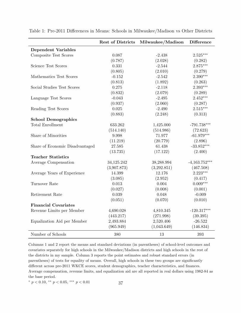
Table 1: Pre-2011 Differences in Means: Schools in Milwaukee/Madison vs Other Districts

Rest of Districts Milwaukee/Madison Difference

Dependent VariablesComposite Test Scores 0.087 -2.438 2.525∗∗∗

(0.787) (2.028) (0.282)Science Test Scores 0.331 -2.544 2.875∗∗∗

(0.805) (2.010) (0.279)Mathematics Test Scores -0.152 -2.542 2.390∗∗∗

(0.813) (1.892) (0.263)Social Studies Test Scores 0.275 -2.118 2.393∗∗∗

(0.832) (2.079) (0.289)Language Test Scores -0.043 -2.495 2.452∗∗∗

(0.937) (2.060) (0.287)Reading Test Scores 0.025 -2.490 2.515∗∗∗

(0.883) (2.248) (0.313)School DemographicsTotal Enrollment 633.262 1,425.000 -791.738∗∗∗

(514.140) (514.986) (72.623)Share of Minorities 9.998 71.977 -61.979∗∗∗

(11.219) (20.779) (2.896)Share of Economic Disadvantaged 27.585 61.438 -33.852∗∗∗

(13.735) (17.122) (2.400)Teacher StatisticsAverage Compensation 34,125.242 38,288.994 -4,163.752∗∗∗

(3,907.873) (3,292.851) (467.508)Average Years of Experience 14.399 12.176 2.223∗∗∗

(3.085) (2.952) (0.417)Turnover Rate 0.013 0.004 0.009∗∗∗

(0.027) (0.008) (0.001)Retirement Rate 0.039 0.048 -0.009

(0.051) (0.070) (0.010)Financial CovariatesRevenue Limits per Member 4,690.028 4,810.345 -120.317∗∗∗

(443.217) (271.998) (39.395)Equalization Aid per Member 2,493.884 2,520.406 -26.522

(965.949) (1,043.649) (146.834)

Number of Schools 380 13 393

Columns 1 and 2 report the means and standard deviations (in parentheses) of school-level outcomes and

covariates separately for high schools in the Milwaukee/Madison districts and high schools in the rest of

the districts in my sample. Column 3 reports the point estimates and robust standard errors (in

parentheses) of tests for equality of means. Overall, high schools in these two groups are significantly

different across pre-2011 WKCE scores, student demographics, teacher characteristics, and finances.

Average compensation, revenue limits, and equalization aid are all reported in real dollars using 1982-84 as

the base period.∗ p < 0.10, ∗∗ p < 0.05, ∗∗∗ p < 0.01 37

Table 2: Pre-2011 Differences in Means: Immediately Treated vs Grandfathered Schools

Immediately Treated Grandfathered Difference

Dependent VariablesComposite Test Scores 0.019 0.035 -0.017

(0.931) (0.829) (0.103)Science Test Scores 0.302 0.236 0.067

(1.040) (0.958) (0.119)Mathematics Test Scores -0.274 -0.136 -0.138

(0.963) (0.845) (0.106)Social Studies Test Scores 0.232 0.263 -0.032

(0.987) (0.871) (0.109)Language Test Scores -0.109 -0.158 0.049

(1.036) (0.834) (0.105)Reading Test Scores -0.057 -0.027 -0.030

(1.024) (0.979) (0.122)School DemographicsTotal Enrollment 631.131 678.765 -47.634

(510.656) (586.001) (72.316)Share of Minorities 9.910 11.874 -1.964

(11.259) (10.235) (1.276)Share of Economic Disadvantaged 27.307 33.539 -6.233∗∗∗

(13.620) (14.903) (1.842)Teacher StatisticsAverage Compensation 34,132.089 33,979.047 153.042

(3,941.712) (3,118.386) (392.053)Average Years of Experience 14.416 14.025 0.392

(3.104) (2.640) (0.330)Turnover Rate 0.013 0.011 0.002

(0.027) (0.027) (0.003)Retirement Rate 0.039 0.036 0.003

(0.051) (0.056) (0.007)Financial CovariatesRevenue Limits per Member 4,688.897 4,714.179 -25.282

(433.617) (617.284) (75.717)Equalization Aid per Member 2,501.899 2,322.736 179.163

(961.975) (1,040.093) (128.631)

Number of Schools 363 17 380

Columns 1 and 2 report the means and standard deviations (in parentheses) of school-level outcomes and

covariates by school type and averaged in the four years preceding the enactment of Act 10 (2007-08

through 2010-11). Column 3 reports the point estimates and robust standard errors (in parentheses) of

tests for equality of means. Average compensation, revenue limits, and equalization aid are all reported in

real dollars using 1982-84 as the base period. Overall, immediately treated and grandfathered schools had

similar WKCE scores, student demographics, teacher characteristics, and finances before Act 10 was

enacted.∗ p < 0.10, ∗∗ p < 0.05, ∗∗∗ p < 0.01 38

Table 3: Differential Effects of Act 32

Equalization Aid Revenue Limits

Post -487.627∗∗∗ -269.808∗∗∗

(13.210) (8.835)Immediately Treated 172.898 -18.557

(254.552) (142.672)Interaction Term 3.463 -0.909

(55.027) (43.451)

N 3,420 3,420

Table tests whether schools in the Immediately Treated and Grandfathered groups were differentially

impacted by Act 32. I am unable to reject the hypothesis that Act 32 affected schools in the two groups in

a similar manner. Standard errors are in parentheses and clustered at the district level.∗ p < 0.10, ∗∗ p < 0.05, ∗∗∗ p < 0.01

39

Table 4: Effects of Act 10 on Student Achievement

Dependent Variable (1) (2) (3) (4) (5)

Composite -0.175∗ -0.190∗∗ -0.217∗∗ -0.202∗∗ -0.153(0.098) (0.093) (0.094) (0.095) (0.103)

Science -0.281∗∗∗ -0.293∗∗∗ -0.320∗∗∗ -0.305∗∗∗ -0.227∗

(0.104) (0.097) (0.091) (0.091) (0.127)Mathematics -0.268∗∗ -0.297∗∗∗ -0.319∗∗∗ -0.310∗∗∗ -0.197∗∗

(0.109) (0.109) (0.116) (0.113) (0.075)Language Arts -0.189∗ -0.196∗ -0.229∗∗ -0.215∗∗ -0.211∗

(0.112) (0.107) (0.102) (0.105) (0.119)Social Studies -0.075 -0.093 -0.117 -0.102 -0.045

(0.135) (0.127) (0.130) (0.132) (0.155)Reading -0.062 -0.072 -0.099 -0.078 -0.086

(0.127) (0.119) (0.118) (0.122) (0.131)

N 3,420 3,420 3,420 3,420 3,420

Year FE X X X X XSchool FE X X X X XWeighted X X X XSchool Demographics X X XFinancial Covariates X XLinear School Trends X

Table reports the estimates, along with standard errors in parentheses and clustered at the district level, of

the effects of Act 10 on student achievement. It shows the robustness of the estimates across five different

specifications. Specifications in columns 2 - 5 are weighted by the school’s (logged) total enrollment. In

columns 3 - 4, I add different sets of covariates: school demographics and financial variables. Finally, in

column 5, I add school-specific linear trends. Overall, the estimates are robust to the specification choice

and indicate that Act 10 reduced WKCE composite test scores by roughly 20% of a standard deviation.

This effect is primarily driven by decreases in science and mathematics test scores, suggesting these

subjects are most responsive to school inputs. Even though all coefficient estimates are negative for social

studies and reading, they are statistically insignificant.∗ p < 0.10, ∗∗ p < 0.05, ∗∗∗ p < 0.01

40

Table 5: Event Study Specification: Estimates of γj’s

Year Composite Science Math Language Social Reading

t-6 -0.005 -0.028 0.136 -0.078 -0.009 -0.046(0.100) (0.101) (0.098) (0.102) (0.133) (0.123)

t-5 0.036 -0.013 0.237∗ -0.046 0.102 -0.099(0.142) (0.142) (0.128) (0.157) (0.169) (0.165)

t-4 0.177 0.178 0.320∗ 0.067 0.172 0.146(0.173) (0.170) (0.174) (0.190) (0.211) (0.182)

t-3 0.065 0.093 0.185 -0.062 0.114 -0.008(0.176) (0.146) (0.194) (0.190) (0.212) (0.182)

t-2 -0.046 -0.012 0.059 -0.104 -0.062 -0.110(0.124) (0.127) (0.116) (0.178) (0.159) (0.121)

t -0.217∗∗ -0.333∗∗∗ -0.293∗∗∗ -0.212∗ -0.126 -0.124(0.091) (0.105) (0.096) (0.123) (0.115) (0.124)

t+1 -0.324∗∗ -0.379∗∗ -0.373 -0.444∗∗ -0.227 -0.199(0.146) (0.159) (0.228) (0.177) (0.148) (0.179)

t+2 -0.345 -0.525∗ -0.440 -0.307 -0.267 -0.189(0.261) (0.309) (0.332) (0.281) (0.273) (0.292)

N 3,420 3,420 3,420 3,420 3,420 3,420

Table presents point estimates, along with standard errors in parentheses and clustered at the district level,

of the γj ’s for each period leading to and immediately after treatment. The year prior to treatment is

omitted so that all estimates are relative to this year. Prior to exposure to the law, all treatment estimates

are statistically insignificant at the 5% level. Following Act 10 exposure, WKCE composite test scores

decrease by approximately 22% of a standard deviation and continue to decrease in the subsequent year, by

roughly 32%. As in Table 4, this effect is primarily driven by decreases in science and mathematics test

scores. The specification is weighted by the school’s (logged) total enrollment. It includes school and year

fixed effects, as well as school demographics and financial covariates as controls.∗ p < 0.10, ∗∗ p < 0.05, ∗∗∗ p < 0.01

41

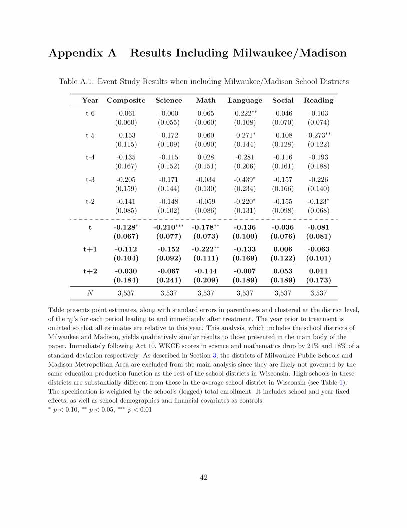
Appendix A Results Including Milwaukee/Madison

Table A.1: Event Study Results when including Milwaukee/Madison School Districts

Year Composite Science Math Language Social Reading

t-6 -0.061 -0.000 0.065 -0.222∗∗ -0.046 -0.103(0.060) (0.055) (0.060) (0.108) (0.070) (0.074)

t-5 -0.153 -0.172 0.060 -0.271∗ -0.108 -0.273∗∗

(0.115) (0.109) (0.090) (0.144) (0.128) (0.122)

t-4 -0.135 -0.115 0.028 -0.281 -0.116 -0.193(0.167) (0.152) (0.151) (0.206) (0.161) (0.188)

t-3 -0.205 -0.171 -0.034 -0.439∗ -0.157 -0.226(0.159) (0.144) (0.130) (0.234) (0.166) (0.140)

t-2 -0.141 -0.148 -0.059 -0.220∗ -0.155 -0.123∗

(0.085) (0.102) (0.086) (0.131) (0.098) (0.068)

t -0.128∗ -0.210∗∗∗ -0.178∗∗ -0.136 -0.036 -0.081(0.067) (0.077) (0.073) (0.100) (0.076) (0.081)

t+1 -0.112 -0.152 -0.222∗∗ -0.133 0.006 -0.063(0.104) (0.092) (0.111) (0.169) (0.122) (0.101)

t+2 -0.030 -0.067 -0.144 -0.007 0.053 0.011(0.184) (0.241) (0.209) (0.189) (0.189) (0.173)

N 3,537 3,537 3,537 3,537 3,537 3,537

Table presents point estimates, along with standard errors in parentheses and clustered at the district level,

of the γj ’s for each period leading to and immediately after treatment. The year prior to treatment is

omitted so that all estimates are relative to this year. This analysis, which includes the school districts of

Milwaukee and Madison, yields qualitatively similar results to those presented in the main body of the

paper. Immediately following Act 10, WKCE scores in science and mathematics drop by 21% and 18% of a

standard deviation respectively. As described in Section 3, the districts of Milwaukee Public Schools and

Madison Metropolitan Area are excluded from the main analysis since they are likely not governed by the

same education production function as the rest of the school districts in Wisconsin. High schools in these

districts are substantially different from those in the average school district in Wisconsin (see Table 1).

The specification is weighted by the school’s (logged) total enrollment. It includes school and year fixed

effects, as well as school demographics and financial covariates as controls.∗ p < 0.10, ∗∗ p < 0.05, ∗∗∗ p < 0.01

42

Appendix B Additional Tables

Table B.1: Distributional Effects of Act 10: High vs Low-Performing Schools

High-Performing Low-Performing

Year Composite Science Math Composite Science Math

t-6 0.098 0.073 0.202∗ -0.085 -0.105 0.081(0.105) (0.099) (0.103) (0.144) (0.145) (0.153)

t-5 0.100 0.021 0.248 0.000 -0.012 0.232(0.175) (0.167) (0.169) (0.191) (0.196) (0.165)

t-4 0.246 0.270 0.420∗ 0.129 0.116 0.236(0.223) (0.243) (0.220) (0.217) (0.202) (0.212)

t-3 0.089 0.078 0.256 0.062 0.125 0.138(0.230) (0.223) (0.217) (0.206) (0.168) (0.240)

t-2 0.083 0.104 0.197∗ -0.144 -0.103 -0.047(0.137) (0.206) (0.119) (0.171) (0.146) (0.170)

t -0.142∗ -0.261 -0.191∗ -0.255∗ -0.368∗∗∗ -0.357∗∗∗

(0.082) (0.159) (0.103) (0.133) (0.115) (0.129)

t+1 -0.055 -0.160 -0.176 -0.499∗∗∗ -0.505∗∗∗ -0.501∗∗

(0.228) (0.307) (0.310) (0.110) (0.105) (0.240)

t+2 -0.225 -0.614 -0.508 -0.382 -0.390 -0.344(0.443) (0.600) (0.486) (0.238) (0.295) (0.358)

N 1,710 1,710 1,710 1,710 1,710 1,710

Table shows the effect of Act 10 on student achievement separately for high and low-performing schools. I

classify as “Low-Performing” schools in the bottom half of the pre-Act 10 composite WKCE distribution,

and as “High-Performing” those in the top half. The results are consistent with those obtained using

quantile regression. The observed negative effect of Act 10 on average student achievement is largely driven

by declines in test scores at initially low-performing schools. The specification is weighted by the school’s

(logged) total enrollment. It includes school and year fixed effects, as well as school demographics and

financial covariates as controls. Standard errors are in parentheses and clustered at the district level.∗ p < 0.10, ∗∗ p < 0.05, ∗∗∗ p < 0.01

43