1

The Economic Consequences of the 2018 US–China Trade Conflict: A CGE

Simulation Analysis*

Hitotsubashi University

Masahiko Tsutsumi**

Abstract

This paper aims at evaluating the economic consequences of the 2018 US–China trade

conflict. The potential impact of the proposed tariff increases is calculated using a global CGE

model. Capital deepening and technological spillover induced by trade are also taken into account

to explore the long-run influence. We can derive the following implications.

First, the additionally imposed tariffs on goods alone declines the GDP in the US and China

by 0.1% and 0.2%, respectively. The equivalent variation in the US and China is reduced by 9.8

billion and 35.2 billion USD, respectively. Although other countries gain from trade diversion,

losses exceed gains globally.

Second, considering the effect from capital deepening and technological spillover induced by

trade makes the situation worse. The GDP in the US and China declines by 1.6% and 2.5%,

respectively. The equivalent variation in the US and China is reduced by 199.5 billion USD and

187.1 billion USD, respectively. Again, the trade diversion is not large enough to recover losses

in these countries.

Third, the imposed tariffs distort relative prices, resulting in changes to the global production

structure. Both the US and China lose their comparative advantage in transport, electronic, and

machinery equipment production, while other countries expand their production in these sectors.

Finally, China’s retaliatory tariff increases worsens the US economy to some extent, but it

comes at a cost to the Chinese economy. In the long run, retaliation is not an appropriate p olicy

response.

Key words: the US, China, Tariff, Trade Policy, Retaliation, CGE model

JEL Classification：F13, F17, F51

* Revised version of CIS Discussion Paper Series, No. 676, Center for Intergenerational Studies, Institute

of Economic Research, Hitotsubashi University, Japan. [http://cis.ier.hit-

u.ac.jp/Common/pdf/dp/2018/dp676.pdf] ** Corresponding address: masahiko223@ier.hit-u.ac.jp. The views expressed in this paper are those of

the author and do not necessarily reflect the views of the Economic Research Institute, Hitotsubashi

University.

2

1. Introduction

In 2018, the United States announced that it would raise tariffs on imports from China. It is

said that there are several reasons for these actions—the continuously large trade deficits, unfair

trade practices and treatment of foreign firms in China, and a lack of adequate legal and

institutional infrastructure to protect intellectual property rights. The Office of the US Trade

Representative (USTR) justified the grounds for the actions by citing article 301 of the 1974 Trade

Act.

The two countries have attempted to resolve these issues in several rounds of negotiations,

but the US decided to impose additional tariffs on Chinese imports anyway to show its serious

intentions. China immediately retaliated with tariff increases on imports from the US. This

situation is now a typical “trade war.”

Many economists and researchers have expressed their concerns over its repercussions on the

regional and global economy using indicative model simulations based on various assumptions.

In line with these studies, this paper aims at exploring the quantitative consequences of the US–

China trade war using a GTAP CGE (Global Trade Analysis Project-Computable General

Equilibrium) model.

2. Measures taken by the US and China

2.1. Tariff increases by the US

According to information released by the US government, the US will impose additional

tariffs on 50 billion USD of imports from China (the sum of 34 billion USD announced on July 6

2018 and 16 billion USD announced on August 23, 2018), followed by the second round of tariff

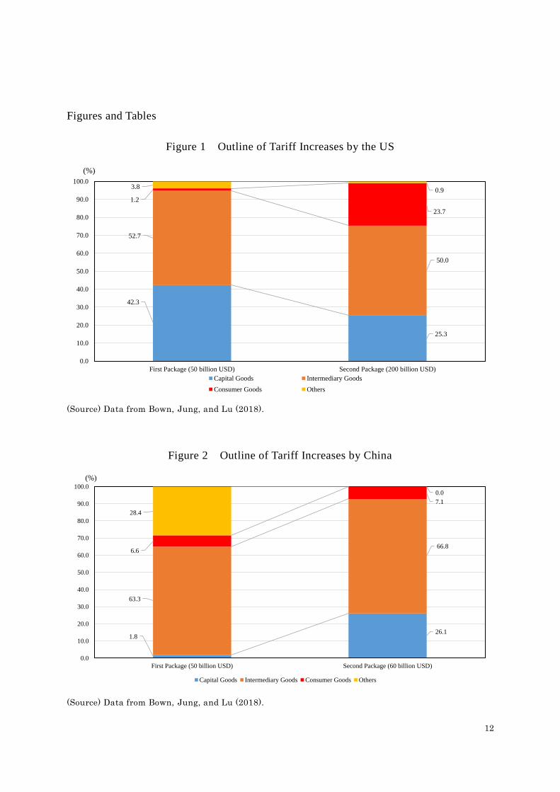
increase on 200 billion USD of imports from China announced on September 24, 2018 (Figure 1).

It is also said that President Trump could impose additional tariffs on the rest of targeted imports—

267 billion USD—depending on the retaliatory actions taken by China.

The additional tariff rate will be set at 25%. The US imports from China was about 505.5

billion USD in 2017, accounting for 21.6% of total US imports. The tariff increases will raise

import prices by 2.7% (25%*49.5%*21.6%), decreasing the GDP deflator by 0.3%. This short-

term impact reflecting a negative economic outlook is well known among economists. Bown, Jung,

and Lu (2018) carefully compared targeted commodities in the first and second bullets and found

that the second bullet contains more consumer goods than the first, resulting in a further negative

impact on consumer prices.

2.2. China

In response to US’ actions, China announced retaliatory measures (Figure 2). The first round

contains tariff increases on 50 billion USD imports from the US (the sum of 34 billion USD

imports announced on July 6 2018 and 16 billion USD imports announced on August 23, 2018).

3

The second round of actions contains tariff increases on 60 billion USD imports from the US.1

The additional tariff rate of the first action is set at 25%, which is the same as the rate imposed

by the US, but the rate for the second action is lower and ranges between 5 and 10%. According

to the analysis by Bown, Jung, and Lu (2018), the lower rate for the second retaliatory action

could reflect the Chinese government’s concern that tariffs would raise intermediary input costs

for domestic firms. The second round of retaliatory action affects capital and investment

commodities, in addition to intermediate input commodities, while the first round of retaliatory

action mainly affects consumer commodities, such as automobiles and food or processed food.

3. Evaluation method

3.1. Previous studies

Previous studies on the US–China trade conflict in 2018 relied on a scenario analysis, due to

the ambiguity in policy decisions and implementation. The International Monetary Fund (IMF,

2018) demonstrated four consecutive scenarios in the US–China trade conflict and its spillover

effects on the world economy. The first two scenarios are based on announced tariff increases by

the US and China, the third scenario includes imaginary additional tariff increases on automobile

imports, and the forth scenario includes negative shocks on the markets or investor sentiment in

general. The first two realistic scenarios indicate that the GDP in the US and emerging Asian

economies, including China, would fall by 0.2 % in the first year, while the GDP in Japan and EU

would increase slightly.2

Similar to the IMF’s simulation, Kobayashi and Hirono (2018b) ran a macroeconomic model

to simulate the potential impact of 10% or 25% tariff increases on the GDP, with two different

fiscal response assumptions—revenue neutral and revenue surplus. The GDP in the US falls by

0.00-0.15% in the 10% increase scenario and by 0.00-0.28% in the 25% increase scenario. The

Chinese GDP falls by 0.01-0.17% in the 10% increase scenario and by 0.05-0.22% in the 25%

increase scenario. They also projected that the GDP in Japan would drop by 0.00-0.02%.

In general, a macroeconomic model simulation helps to understand how tariff increases affect

prices, including exchange rates and final demand. Further, it would be possible to trace a possible

overshoot impact on financial variables by taking into account a reasonable scenario in investor

sentiment, albeit ad hoc. However, a macroeconomic model fails to capture industry-level change

due to data aggregation. It also has a limitation in assessing the long-run impact on supply capacity.

A general equilibrium model with a trade matrix has the comparative advantage in dealing with

these aspects; therefore, it is more appropriate for use in quantification of trade issues.

1 The first and second measures by China are addressed in the following announcements. For the first

action, see http://gss.mof.gov.cn/zhengwuxinxi/zhengcefabu/201806/t20180616_2930325.html . For the

second action, see http://gss.mof.gov.cn/zhengwuxinxi/zhengcefabu/201808/t20180808_2983770.html . 2 Kobayashi and Hirono (2018a) compares projections by international organizations and their institute.

4

For example, Rosyadi and Widodo (2018) conducted a simulation using a standard GTAP

model with dataset version 9.0, to evaluate the US–China trade dispute. Their simulation shows

comparative statics, with labor mobility among sectors within a country. In the first scenario, US

import tariffs are raised by 45% on all imports from China and Chinese import tariffs are raised

by a certain level to reach an ex-post rate of 45%.3 The second scenario excludes agricultural

products from the first scenario. Since the US had already announced the additional tariff rate

would be 25%, the assumed rate of 45% lost its meaning. However, we can still use the result as

a multiplier as long as the results are linear with tariff increases. In the first scenario, both the US

and China’s GDP falls by 1.22% and 5.4%, respectively. Thus, we can speculate that a 25% hike

in tariffs would decrease their GDP by 0.7% and 3.0%, respectively.

Li, He, and Lin (2018) calibrated their original CGE model to calculate welfare changes

caused by tariff increases by the US and China. Their model has 29 countries or regions with

tradable and non-tradable goods and 2013 as the benchmark year. When respective tariffs on

imports between the US and China are increased by 15%, the GDP in the US increases by 0.007%

while in China, it falls by 0.667%. In the scenario where respective tariffs on imports are increased

by 30%, again, the GDP in the US increases by 0.037% while in China, it falls by 1.152%.

Although it is not clear why the GDP in the US increases, one could conjecture that a higher price

of tradable goods might stimulate domestic production, which would generate an additional

income effect for non-tradable goods. From these simulation exercises, they concluded that the

US–China trade conflict is a non-cooperative Nash equilibrium, indicating the US can gain from

unilateral tariff increases, and China can reduce its losses by retaliating.

Bollen and Rojas-Romagosa (2018) demonstrated seven scenario simulations using the

WorldScan CGE model developed by the Netherlands Bureau for Economic Policy Analysis. One

of the seven scenarios includes the US–China tariff increases. According to their results, the GDP

in the US and China falls by 0.3% and 1.2%, respectively, compared to the baseline in 2030. Note

that their simulation only considers the tariff increases announced in July 2018 and does not take

into account the additional measures announced in September 2018.

3.2. Data and Model

3.2.1. Data

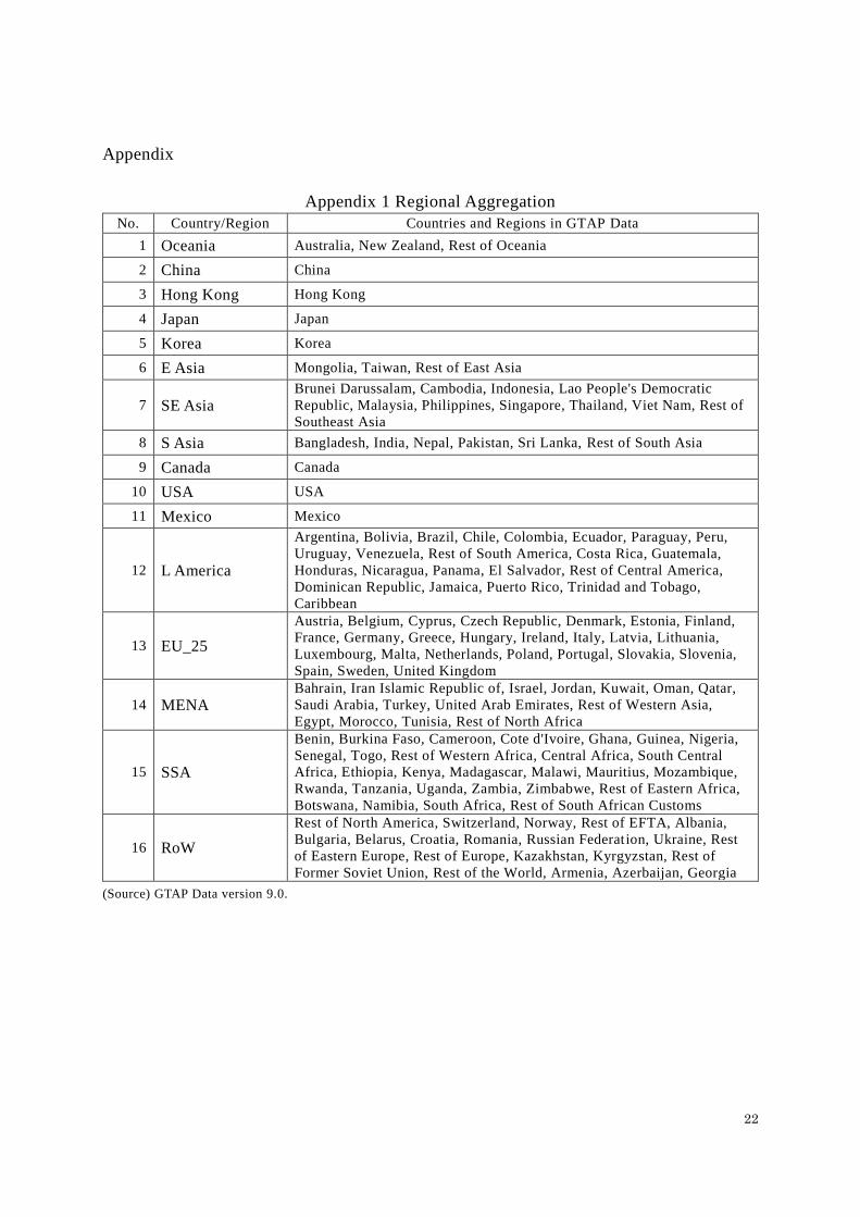
In this paper, we use GTAP data version 9.0 (R9p1_2011_Mar2014). This is the same version

dataset used in the two previous studies—Rosyadi and Widodo (2018) and Bollen and Rojas-

Romagosa (2018) but released earlier than the final. The benchmark year is 2011 but the national

accounts data and trade statistics are adjusted to replicate the balance among regions. 4 The

original database consists of 140 countries or regions and 57 commodities or industries. For our

analytical purposes, it is aggregated into 16 countries or regions and 12 commodities or industries

3 Authors argue that a large trade diversion and deterioration of terms of trade happen, however, it is not

explicitly shown how much China will raise its tariffs on imports from the US to achieve the ex-post

rate of 45%. 4 For a detailed account of this issue, see GTAP technical paper series on data construction.

5

(see Appendix 1 and Appendix 2). There are five initial endowments for production—land,

unskilled labor, skilled labor, and natural resources.

3.2.2. Model

Our model is version 6.2 of the GTAP models, with an additional equation to link trade

openness and technological changes. The following section briefly explains the basic structure of

the model.5

In our model, there is a social welfare function composed of private consumption, government

consumption, and national savings. Since the function takes the form of Cobb-Douglas, each share

is held constant. Each commodity demand of private consumption is driven by income, relative

prices, and initial quantity of demand. Domestic demand is comprised of domestic supply and

aggregate imports, which are elastic to relative price changes.

Firms are assumed to produce commodities by mixing value-added and intermediary inputs.

The value-added inputs are land, labor, capital, and natural resources, and their composition

weights vary by industry. The intermediary inputs are determined by fixed proportion to output—

the Leontief structure. The intermediary inputs are also composed of domestic supply and

aggregate imports.

Substitution between domestic and imported goods is determined by the fixed elasticity of

substitution. Among the import destinations, the same substitution structure with different

elasticity is assumed (Appendix 3).

The national savings rate is fixed by the Cobb-Douglas type social utility function. While

national investment is derived from production activities, the gap between savings and investment

equals net imports. To solve the model, it is assumed that national investment is allocated to

equalize the expected rate of return on capital among regions.

One equation is added to the standard model for this exercise, a link between trade openness

and nationwide technological change. It aims at capturing the economic impact argued in the

previous studies on trade and technological spillover effects. It is often claimed that trade

openness nurtures innovation through creating a competitive environment for firms, meaning a

higher degree of diversity in goods and firms in the markets. For example, Lee et.al (2004) analyze

a relation between per capita growth and trade openness and conclude that a 10 percentage point

hike in trade openness brings 0.27% growth. Also, Wolszczak-Derlacz (2014) show a positive

relationship between Total Factor Productivity (TFP) and trade openness through competitive

environment by panel data of OECD countries. Although this is an ad hoc treatment, it is worth

taking the explicit link between trade and technology into account (Appendix 4).6

5 For a detailed account of models and data of the GTAP, see the latest website information on

https://www.gtap.agecon.purdue.edu/models/current.asp. Note that 7 is the latest version of the model. 6 The formula is AOREG=0.15＊(gross trade change – GDP change). See Government Headquarters for

6

3.3. Simulation plan

The economic impact of the US and China’s tariff increases is calculated using different

macroeconomic closures to analyze the three causes of changes. The primary cause is tariff

increases. Kobayashi and Hirono (2018b) and Bown, Jung, and Lu (2018) used the information

released by government and trade statistics to construct a dataset at HS code (Harmonized

Commodity Description and Coding System) 2- or 6- digit levels.

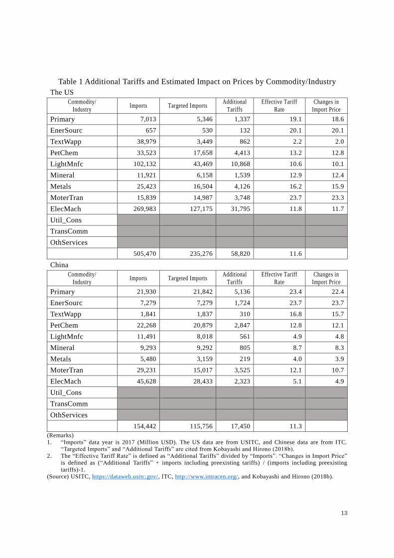
Based on their studies and the tariff data in GTAP version 9.0, the effective additional changes

in tariff rates and import prices are calculated in Table 1. According to this exercise, the effective

additional tariff rates in China are uneven by commodity, reflecting a difference in the first and

second round of retaliation. The average change rate is not too different from that of the US,

although China targets a larger portion of total imports compared to the US.

The second cause is capital accumulation. The primary change by tariff increases influences

commodity prices and quantity, and renews income, savings, and investment. Changes in savings

are, by definition, changes in capital accumulation in the long-run. The third cause is the

technological change induced by trade. As noted in the previous section, an ad hoc equation is

incorporated to capture the trade induced technological change on the whole economy.

4. The economic consequences of trade war

4.1. Impact of tariff increases

4.1.1. Key macroeconomic indicators

The changes in key macroeconomic indicators by tariff increases alone are presented in Table

2. The imports and exports in both the US and China drop significantly, while trade diversion

effects allow the imports and exports in other countries and regions to grow to some extent. The

world trade volume drops by 0.6%. The terms of trade (export price/import price) of China

deteriorates, while that of the US is not significantly affected. A small improvement in terms of

trade with Canada and Mexico is found.

The changes in the terms of trade also influence the domestic economic variables—

production and income. The GDP in the US and China drops by 0.1% and 0.2%, respectively,

while other countries and regions slightly gain through trade diversion effects. The world GDP

declines slightly by 0.03%. Looking at the equivalent variation, losses in the US and China amount

to 9.8 billion USD and 35.2 billion USD, respectively, resulting in 23.9 billion USD losses globally.

In this simulation, the expected return on capital in each country is equalized to the global

rate of return on capital such that the IS gap would change. The trade deficits in the US and the

trade surplus in China shrinks, as was intended by the US administration. However, it is just by

15 billion USD, which accounts for 3.5% of Chinese surplus or 1.9% of the US deficits. It is

the TPP, Japan (2015).

7

suggested that changing the trade balance through tariffs does not make sense given the large cost

incurred.

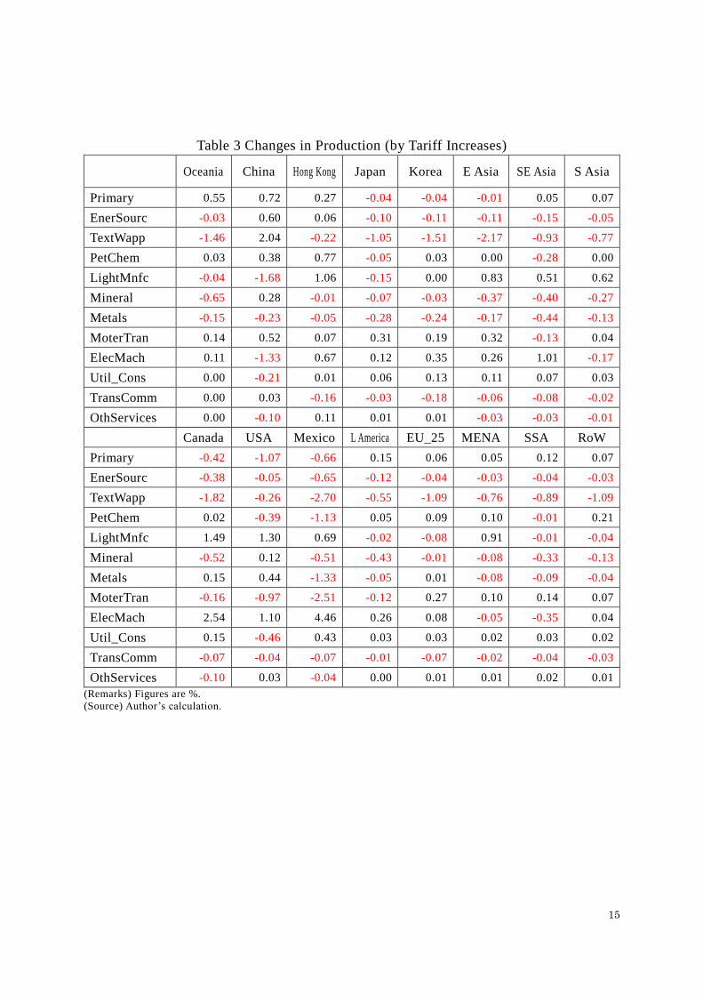
4.1.2. Production by industry

The changes in industrial production are presented in Table 3. In the US, the light-

manufacturing sector (LightMnfc), and electronic and machinery equipment sector (ElecMach)

expand, while the agriculture and processed food sector (Primary), and motor vehicles and parts,

transport equipment sector (MoterTran) declines. In China, the opposite changes occur—

expansion in Primary and contraction in ElecMach.

There are several steps for effecting change from tariff increases to industrial production.

First, in the country that raises the tariffs, the import prices from the targeted country increase so

the relative import prices from other countries are lowered. As a result, imports from other

countries substitute the imports from the targeted country. Second, even if substitution works, the

average import price inevitably increases, so the domestic prices are relatively lowered to the

average import price level. This drives domestic products to substitute imports, allowing an

expansion in domestic production. The reduced demand for aggregate imports is then reallocated

among the trading countries. Thus, the final effect of tariff increases contains not only a direct

substitution among competitive exporters, but also an indirect substitution with domestic

producers.

It is also important that changes in intermediary input price affect domestic production. In

this case, the Chinese MoterTran is slapped with additional 23.7% tariffs on its products by the

US, but the output expands by 0.5%. On the contrary, when the US MoterTran is imposed with

additional 12.1% tariffs on its products by China, the output declines by 1%. At a glance, the

protection levels are not consistent with output results in both countries. One of the reasons why

the US MoterTran production declines could be the higher tariffs on intermediary inputs for the

MoterTran—steel and metal (Metals), and ElecMach. While additional tariff on Metals imports in

China is 4%, it is 16.2% in the US. Further, additional tariffs on ElecMach imports is 5.1% and

11.8% in China and the US, respectively. The domestic production of both in the US expand, but

the US MoterTran has to use the intermediary inputs at higher prices, resulting in losing

competitiveness in the global market.

The changes in production are not affected by a direct substitution with the third country

caused by tariff increases in the US and China, but are affected by changes in production cost

caused by tariff increases in other sectors. The relative price changes induced by tariffs also affect

the comparative advantage of each country, resulting in an expansion and contraction at the

sectoral levels.

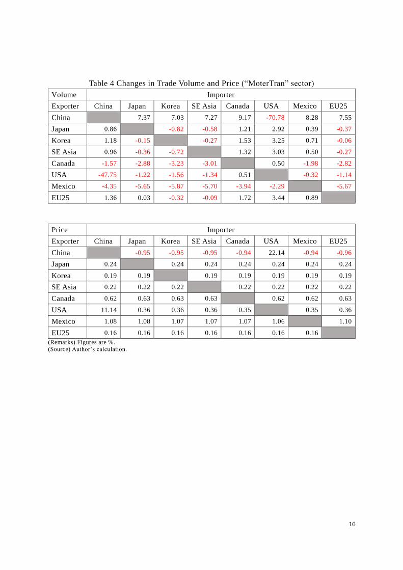
4.1.3. Trade volume and price by industry

In Table 4, the changes in bilateral trade volume and prices in MoterTran are presented to

show how changes in intermediary input costs and production are related. According to the

8

simulation results for 8 countries out of the total 16 countries, the exports from China to the US

falls by more than 70%, while the exports to other countries, on average, increase by 7–9 %.

Whereas, the exports from the US not only falls by 50% to China, but also to other countries as

well.

The reason the export performance of MoterTran in the two countries differs is because of

changes in prices. The price of MoterTran from China in the US increases by 22% due to a hike

in tariffs, but the price of the same products in other countries decreases thanks to a fall in

production cost within China. Hence, an improved price competitiveness expands exports. On the

contrary, the price of MoterTran from the US not only increases by 11% in China due to a hike in

tariffs, but also increases in other countries due to a hike in production cost. Hence, the worsened

price competitiveness contracts exports.

4.2. Impact of capital deepening and trade induced technology

4.2.1. Key macroeconomic indicators

The simulation exercise to demonstrate the effect of tariff increases alone shows that the

bilateral measures to raise tariffs alter the comparative advantage among sectors in both countries

with losses from distortion. It also proves that tariff increases do not change the levels of trade

balance much and its spillover effect to the third country is marginal.

Although the short-term impact would not be significant, the changes in production and

income should affect the long-term growth potential through savings and technological spillover

induced by trade. In Table 5, the simulation results including capital deepening and trade induced

technological changes are presented. As expected, the trade volume in the US and China decreases

further and trade diversion effects become larger. The world trade declines by 0.6%, which is

almost the same as in the previous case. The changes in the terms of trade become smaller, since

a part of price changes are absorbed by the changes in real variables— capital stock and production.

The GDP in the US and China declines by 1.6% and 2.5%, respectively.

In the third country, trade diversion effects allow it to boost income and investment, resulting

in growth of capital stock, but the world GDP falls by 0.45%. The changes in equivalent variation

in the US and China worsen by 199.5 billion and 187.1 billion USD, respectively, while the third

countries gain marginally. The world total remains negative, recording losses of 287.2 billion USD.

Since the real variables move more, the changes in trade balance are smaller than in the previous

case.

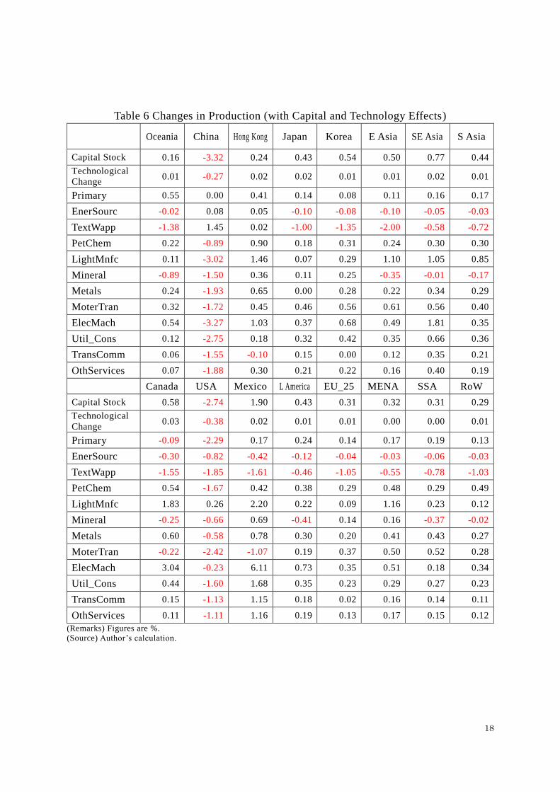
4.2.2. Production by industry

The output changes by industry are shown in Table 6. Capital stock in the US and China falls

by 2.7% and 3.3%, respectively due to a fall in income and investment. The long-term growth

potential is lost permanently because of tariff increases.

In the US, only LightMnfc production expands. Among the other sectors, the worst affected

is MoterTran, contracting by 2.5%. In China, only two sectors—fuel (EnerSourc) and textile and

9

apparel (TextWapp) expand, while others contract. The worst affected is ElecMach, contracting by

3%.

These changes are generated by a dynamic mechanism between income, investment , and

capital accumulation. In the long run, decreased investment weakens capital accumulation,

resulting in a lower capital-labor ratio in the two countries. Further, a smaller trade volume brings

poorer technological innovation to the economy as a whole, decreasing the growth potential.

4.2.3. Contribution of endogenous growth mechanisms

The two simulation cases suggest that the indirect effects from capital deepening and trade

induced technological change are more significant than the direct effects from tariff increases. In

Table 7, the contribution rate of four factors—tariffs, capital change, technological change, and

cross-term—to total changes are shown.

In many countries, among four factors, “trade induced technological changes” contributes the

maximum towards a change in the GDP. The contribution rate of “trade induced technological

change” reaches 50% in Australia and China. It reaches 40% in the US and 30% in Hong Kong

and Canada. “Capital deepening” contributes significantly in Mexico, almost 80%. It also

contributes more than 50% in the Asian countries, excluding Japan and Hong Kong. The level of

contribution from these two factors are affected by the initial conditions in the respective countries.

As equivalent variations contain the effect from price changes, the contribution from “tariff

increases” rises. In Hong Kong, East Asia, and Canada, 50% of total changes are attributable to

“tariff increases.” The contribution from “capital deepening” is again high in Mexico, East Asia,

Southeast Asia, and South Asia. “Trade induced technological change” contributes significantly

in Oceania, China, Japan, the US, Middle and South America, the EU, Middle East, and North

Africa. The combination of source of changes varies by region.

5. Conclusion

5.1. Efficacy of retaliation

We examined the economic consequences of trade measures taken by both the US and China

and confirmed that tariff increases would negatively affect both economies. Did China have to

retaliate against the US this time? Is its action effective in mitigating the negative impact of the

action taken by the US, or in preempting the US from taking further punitive actions? These

questions are answered here based on the simulation results.

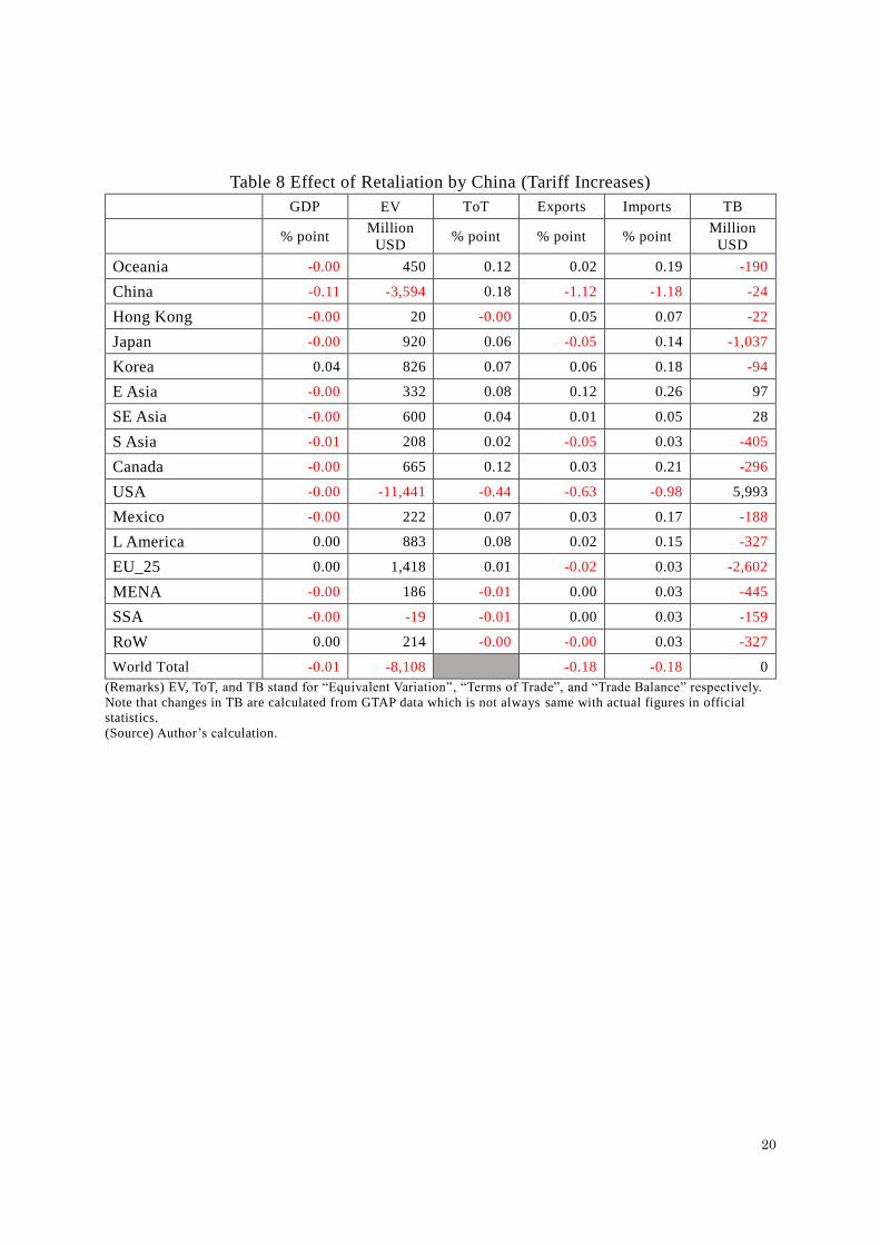
The effect of China’s retaliatory measures and their effect, including capital deepening and

trade induced technological changes are shown in Table 8 and Table 9, respectively. The GDP in

the US falls by 0.00% points or 0.24% points, while the GDP in China falls by 0.11% points or

0.88% points. The equivalent variation in the US worsens by 11.4–40.4 billion USD, while in

China it worsens by 3.6–55.9 billion USD.

10

At first glance, the retaliation induces losses of 11.4 billion USD in the US at the cost of 3.6

billion USD loss in China. Although this is not a welfare enhancing case as Li et. al. (2018) argue,

it does seem to be a cost-effective measure according to the relative changes in equivalent

variations. Having said that, one would find that another long-run simulation would show different

results. The retaliation not only decreases the US GDP by 0.24% and equivalent variations by 40.4

billion USD, but it also decreases the Chinese GDP by 0.88% and equivalent variations by 55.9

billion USD. Eventually, China will lose more than the US.

5.2. Concluding remarks

This paper aims at evaluating the economic consequences of the 2018 US–China trade

conflict. The potential impact of the proposed tariff increases is calculated using a global CGE

model. Capital deepening and technological spillover induced by trade are also taken into account

to explore the long-run influence. We can derive the following implications.

First, the additionally imposed tariffs on goods alone declines the GDP in the US and China

by 0.1% and 0.2%, respectively. The equivalent variation in the US and China is reduced by 9.8

billion and 35.2 billion USD, respectively. Although other countries gain from trade diversion,

losses exceed gains globally.

Second, considering the effect from capital deepening and technological spillover induced by

trade makes the situation worse. The GDP in the US and China declines by 1.6% and 2.5%,

respectively. The equivalent variation in the US and China is reduced by 199.5 billion USD and

187.1 billion USD, respectively. Again, the trade diversion is not large enough to recover losses

in these countries.

Third, the imposed tariffs distort relative prices, resulting in changes to the global production

structure. Both the US and China lose their comparative advantage in transport, electronic, and

machinery equipment production, while other countries expand their production in these sectors.

Finally, China’s retaliatory tariff increases worsens the US economy to some extent, but it

comes at a cost to the Chinese economy. In the long run, retaliation is not an appropriate policy

response.

11

［Bibliography］

Bollen, Johannes and Hugo Rojas-Romagosa (2018), “Trade Wars: Economic impacts of US tariff

increases and retaliations. An international perspective”, CPB Background Document, July

2018. [CPB-Background-Document-July2018-Trade-Wars-update.pdf]

Bown, Chad P., Euijin Jung, and Zhiyao (Lucy) Lu (2018), “Trump and China Formalize Tariffs on

$260 Billion of Imports and Look Ahead to Next Phase,” September 20, 2018.

[https://piie.com/blogs/trade-investment-policy-watch/trump-and-china-formalize-tariffs-260-

billion-imports-and-look]

Government Headquarters for the TPP, Japan (2015), “TPP Kyoutei no Keizaikoukabunseki,”

Cabinet Secretariat, the Government of Japan, (Tokyo: December 24, 2015).

[http://www.cas.go.jp/jp/tpp/kouka/pdf/151224/151224_tpp_keizaikoukabunnseki02.pdf] (In

Japanese).

Kobayashi, Shun-suke, and Hirono, Kota (2018a), “Zoku Beicyu-tsushosenso no Impact Shisan –

Daiwasoken Shisan v.s. Kokusaikikan Shisan,” Daiwa Research Institute, (Tokyo: July 20,

2018). [https://www.dir.co.jp/report/research/economics/japan/20180720_020214.pdf] (In

Japanese)

Kobayashi, Shun-suke, and Hirono, Kota (2018b), “Saishinsaisoku Beicyu-bouekisenso nitomonau

“Hinmokubetu” Tsuikakanzeiritu no Shosaibunseki,” Daiwa Research Institute, (Tokyo:

September 20, 2018)

[https://www.dir.co.jp/report/research/economics/japan/20180920_020326.pdf] (In Japanese).

Lee, Ha Yan, Luca Antonio Ricci, and Roberto Rigobon (2004), “Once Again, is Openness Good for

Growth?” IMF Working Papers, WP/04/135, Washington D.C.

[http://www.imf.org/external/pubs/ft/wp/2004/wp04135.pdf]

Li, Chunding, He, Chuantian, and Chuangwei Lin (2018), “Economic Impacts of the Possible China–

US Trade War,” Emerging Markets Finance & Trade, 54:1557–1577, 2018.

[https://doi.org/10.1080/1540496X.2018.1446131]

Office of the United States Trade Representative (USTR) (2018), Findings of the Investigation into

China’s Acts, Policies, and Practices related to Technology Transfer, Intellectual Property, and

Innovation under Section 301 of the Trade Act of 1974, March 22, 2018.

[https://ustr.gov/sites/default/files/Section%20301%20FINAL.PDF]

Rosyadi, Saiful Alim, and Tri Widodo (2018), “Impact of Donald Trump’s tariff increase against

Chinese imports on global economy: Global Trade Analysis Project (GTAP) model,” Journal of

Chinese Economic and Business Studies, 16:2, 125-145, 2018.

[DOI:10.1080/14765284.2018.1427930]

The International Monetary Fund (IMF) (2018), “G-20 Surveillance Note,” G-20 Finance Ministers

and Central Bank Governors’ Meetings, (Buenos Aires: July 21-22, 2018).

[https://www.imf.org/external/np/g20/pdf/2018/071818.pdf]

Wolszczak-Derlacz, Joanna (2014), “The Impact of Domestic and Foreign Competition On Sectoral

Growth: A Cross-Country Analysis.” Bulletin of Economic Research. 66 (S1) S110-S131.

12

Figures and Tables

Figure 1 Outline of Tariff Increases by the US

(Source) Data from Bown, Jung, and Lu (2018).

Figure 2 Outline of Tariff Increases by China

(Source) Data from Bown, Jung, and Lu (2018).

42.3

25.3

52.7

50.0

1.2

23.7

3.80.9

0.0

10.0

20.0

30.0

40.0

50.0

60.0

70.0

80.0

90.0

100.0

First Package (50 billion USD) Second Package (200 billion USD)

Capital Goods Intermediary Goods

Consumer Goods Others

(%)

1.826.1

63.3

66.86.6

7.1

28.4

0.0

0.0

10.0

20.0

30.0

40.0

50.0

60.0

70.0

80.0

90.0

100.0

First Package (50 billion USD) Second Package (60 billion USD)

Capital Goods Intermediary Goods Consumer Goods Others

(%)

13

Table 1 Additional Tariffs and Estimated Impact on Prices by Commodity/Industry

The US

Commodity/

Industry Imports Targeted Imports

Additional

Tariffs

Effective Tariff

Rate

Changes in

Import Price

Primary 7,013 5,346 1,337 19.1 18.6

EnerSourc 657 530 132 20.1 20.1

TextWapp 38,979 3,449 862 2.2 2.0

PetChem 33,523 17,658 4,413 13.2 12.8

LightMnfc 102,132 43,469 10,868 10.6 10.1

Mineral 11,921 6,158 1,539 12.9 12.4

Metals 25,423 16,504 4,126 16.2 15.9

MoterTran 15,839 14,987 3,748 23.7 23.3

ElecMach 269,983 127,175 31,795 11.8 11.7

Util_Cons

TransComm

OthServices

505,470 235,276 58,820 11.6

China

Commodity/

Industry Imports Targeted Imports

Additional

Tariffs

Effective Tariff

Rate

Changes in

Import Price

Primary 21,930 21,842 5,136 23.4 22.4

EnerSourc 7,279 7,279 1,724 23.7 23.7

TextWapp 1,841 1,837 310 16.8 15.7

PetChem 22,268 20,879 2,847 12.8 12.1

LightMnfc 11,491 8,018 561 4.9 4.8

Mineral 9,293 9,292 805 8.7 8.3

Metals 5,480 3,159 219 4.0 3.9

MoterTran 29,231 15,017 3,525 12.1 10.7

ElecMach 45,628 28,433 2,323 5.1 4.9

Util_Cons

TransComm

OthServices

154,442 115,756 17,450 11.3

(Remarks)

1. “Imports” data year is 2017 (Million USD). The US data are from USITC, and Chinese data are from ITC.

“Targeted Imports” and “Additional Tariffs” are cited from Kobayashi and Hirono (2018b).

2. The “Effective Tariff Rate” is defined as “Additional Tariffs” divided by “Imports”. “Changes in Import Price”

is defined as (“Additional Tariffs” + imports including preexisting tariffs) / (imports including preexisting

tariffs)-1.

(Source) USITC, https://dataweb.usitc.gov/, ITC, http://www.intracen.org/, and Kobayashi and Hirono (2018b).

14

Table 2 Changes in Key Indicators (by Tariff Increases) GDP EV ToT Exports Imports TB

% point Million

USD % point % point % point

Million

USD

Oceania 0.00 151 0.12 0.14 0.23 72

China -0.21 -35,217 -1.23 -3.46 -4.94 -15,194

Hong Kong 0.00 158 0.11 0.13 0.24 4

Japan 0.00 2,280 0.30 0.24 0.66 -660

Korea 0.03 1,271 0.23 0.22 0.53 -72

E Asia 0.00 526 0.19 0.19 0.43 235

SE Asia 0.01 2,281 0.22 0.29 0.48 666

S Asia 0.01 900 0.16 0.28 0.34 -65

Canada 0.02 2,349 0.47 0.58 1.11 -346

USA -0.09 -9,816 0.09 -3.61 -3.04 15,335

Mexico 0.03 3,107 0.93 0.56 1.69 27

L America 0.02 1,775 0.20 0.27 0.45 265

EU_25 0.01 4,645 0.07 0.08 0.16 -772

MENA 0.01 554 0.05 0.12 0.16 204

SSA 0.02 561 0.10 0.14 0.22 1

RoW 0.01 557 0.07 0.08 0.14 299

World Total -0.03 -23,919 -0.56 -0.56 0

(Remarks) EV, ToT, and TB stand for “Equivalent Variation”, “Terms of Trade”, and “Trade Balance” respectively.

Note that changes in TB are calculated from GTAP data which is not always same with actual figures in official

statistics.

(Source) Author’s calculation.

15

Table 3 Changes in Production (by Tariff Increases)

Oceania China Hong Kong Japan Korea E Asia SE Asia S Asia

Primary 0.55 0.72 0.27 -0.04 -0.04 -0.01 0.05 0.07

EnerSourc -0.03 0.60 0.06 -0.10 -0.11 -0.11 -0.15 -0.05

TextWapp -1.46 2.04 -0.22 -1.05 -1.51 -2.17 -0.93 -0.77

PetChem 0.03 0.38 0.77 -0.05 0.03 0.00 -0.28 0.00

LightMnfc -0.04 -1.68 1.06 -0.15 0.00 0.83 0.51 0.62

Mineral -0.65 0.28 -0.01 -0.07 -0.03 -0.37 -0.40 -0.27

Metals -0.15 -0.23 -0.05 -0.28 -0.24 -0.17 -0.44 -0.13

MoterTran 0.14 0.52 0.07 0.31 0.19 0.32 -0.13 0.04

ElecMach 0.11 -1.33 0.67 0.12 0.35 0.26 1.01 -0.17

Util_Cons 0.00 -0.21 0.01 0.06 0.13 0.11 0.07 0.03

TransComm 0.00 0.03 -0.16 -0.03 -0.18 -0.06 -0.08 -0.02

OthServices 0.00 -0.10 0.11 0.01 0.01 -0.03 -0.03 -0.01

Canada USA Mexico L America EU_25 MENA SSA RoW

Primary -0.42 -1.07 -0.66 0.15 0.06 0.05 0.12 0.07

EnerSourc -0.38 -0.05 -0.65 -0.12 -0.04 -0.03 -0.04 -0.03

TextWapp -1.82 -0.26 -2.70 -0.55 -1.09 -0.76 -0.89 -1.09

PetChem 0.02 -0.39 -1.13 0.05 0.09 0.10 -0.01 0.21

LightMnfc 1.49 1.30 0.69 -0.02 -0.08 0.91 -0.01 -0.04

Mineral -0.52 0.12 -0.51 -0.43 -0.01 -0.08 -0.33 -0.13

Metals 0.15 0.44 -1.33 -0.05 0.01 -0.08 -0.09 -0.04

MoterTran -0.16 -0.97 -2.51 -0.12 0.27 0.10 0.14 0.07

ElecMach 2.54 1.10 4.46 0.26 0.08 -0.05 -0.35 0.04

Util_Cons 0.15 -0.46 0.43 0.03 0.03 0.02 0.03 0.02

TransComm -0.07 -0.04 -0.07 -0.01 -0.07 -0.02 -0.04 -0.03

OthServices -0.10 0.03 -0.04 0.00 0.01 0.01 0.02 0.01

(Remarks) Figures are %.

(Source) Author’s calculation.

16

Table 4 Changes in Trade Volume and Price (“MoterTran” sector)

Volume Importer

Exporter China Japan Korea SE Asia Canada USA Mexico EU25

China 7.37 7.03 7.27 9.17 -70.78 8.28 7.55

Japan 0.86 -0.82 -0.58 1.21 2.92 0.39 -0.37

Korea 1.18 -0.15 -0.27 1.53 3.25 0.71 -0.06

SE Asia 0.96 -0.36 -0.72 1.32 3.03 0.50 -0.27

Canada -1.57 -2.88 -3.23 -3.01 0.50 -1.98 -2.82

USA -47.75 -1.22 -1.56 -1.34 0.51 -0.32 -1.14

Mexico -4.35 -5.65 -5.87 -5.70 -3.94 -2.29 -5.67

EU25 1.36 0.03 -0.32 -0.09 1.72 3.44 0.89

Price Importer

Exporter China Japan Korea SE Asia Canada USA Mexico EU25

China -0.95 -0.95 -0.95 -0.94 22.14 -0.94 -0.96

Japan 0.24 0.24 0.24 0.24 0.24 0.24 0.24

Korea 0.19 0.19 0.19 0.19 0.19 0.19 0.19

SE Asia 0.22 0.22 0.22 0.22 0.22 0.22 0.22

Canada 0.62 0.63 0.63 0.63 0.62 0.62 0.63

USA 11.14 0.36 0.36 0.36 0.35 0.35 0.36

Mexico 1.08 1.08 1.07 1.07 1.07 1.06 1.10

EU25 0.16 0.16 0.16 0.16 0.16 0.16 0.16

(Remarks) Figures are %.

(Source) Author’s calculation.

17

Table 5 Changes in Key Indicators (with Capital and Technology Effects) GDP EV ToT Exports Imports TB

% point Million

USD % point % point % point

Million

USD

Oceania 0.07 728 0.03 0.09 0.21 -276

China -2.46 -187,060 -1.07 -4.20 -6.11 -8,204

Hong Kong 0.17 291 -0.03 0.24 0.24 -25

Japan 0.23 12,654 0.26 0.34 0.72 -495

Korea 0.27 3,052 0.17 0.42 0.66 236

E Asia 0.22 1,168 0.12 0.34 0.50 515

SE Asia 0.46 10,232 0.15 0.68 0.92 -27

S Asia 0.23 5,171 0.15 0.29 0.55 -1,599

Canada 0.29 5,282 0.25 0.63 0.99 -534

USA -1.60 -199,473 0.35 -4.52 -3.53 14,735

Mexico 1.25 14,394 0.54 1.67 2.36 569

L America 0.22 9,780 0.13 0.28 0.55 -1,007

EU_25 0.15 24,244 0.06 0.19 0.29 -2,189

MENA 0.20 5,982 -0.04 0.23 0.29 -926

SSA 0.16 1,698 -0.01 0.24 0.29 -416

RoW 0.14 4,687 0.02 0.18 0.29 -358

World Total -0.45 -287,172 -0.61 -0.61 0

(Remarks) EV, ToT, and TB stand for “Equivalent Variation”, “Terms of Trade”, and “Trade Balance” respectively.

Note that changes in TB are calculated from GTAP data which is not always same with actual figures in official

statistics.

(Source) Author’s calculation.

18

Table 6 Changes in Production (with Capital and Technology Effects)

Oceania China Hong Kong Japan Korea E Asia SE Asia S Asia

Capital Stock 0.16 -3.32 0.24 0.43 0.54 0.50 0.77 0.44

Technological

Change 0.01 -0.27 0.02 0.02 0.01 0.01 0.02 0.01

Primary 0.55 0.00 0.41 0.14 0.08 0.11 0.16 0.17

EnerSourc -0.02 0.08 0.05 -0.10 -0.08 -0.10 -0.05 -0.03

TextWapp -1.38 1.45 0.02 -1.00 -1.35 -2.00 -0.58 -0.72

PetChem 0.22 -0.89 0.90 0.18 0.31 0.24 0.30 0.30

LightMnfc 0.11 -3.02 1.46 0.07 0.29 1.10 1.05 0.85

Mineral -0.89 -1.50 0.36 0.11 0.25 -0.35 -0.01 -0.17

Metals 0.24 -1.93 0.65 0.00 0.28 0.22 0.34 0.29

MoterTran 0.32 -1.72 0.45 0.46 0.56 0.61 0.56 0.40

ElecMach 0.54 -3.27 1.03 0.37 0.68 0.49 1.81 0.35

Util_Cons 0.12 -2.75 0.18 0.32 0.42 0.35 0.66 0.36

TransComm 0.06 -1.55 -0.10 0.15 0.00 0.12 0.35 0.21

OthServices 0.07 -1.88 0.30 0.21 0.22 0.16 0.40 0.19

Canada USA Mexico L America EU_25 MENA SSA RoW

Capital Stock 0.58 -2.74 1.90 0.43 0.31 0.32 0.31 0.29

Technological

Change 0.03 -0.38 0.02 0.01 0.01 0.00 0.00 0.01

Primary -0.09 -2.29 0.17 0.24 0.14 0.17 0.19 0.13

EnerSourc -0.30 -0.82 -0.42 -0.12 -0.04 -0.03 -0.06 -0.03

TextWapp -1.55 -1.85 -1.61 -0.46 -1.05 -0.55 -0.78 -1.03

PetChem 0.54 -1.67 0.42 0.38 0.29 0.48 0.29 0.49

LightMnfc 1.83 0.26 2.20 0.22 0.09 1.16 0.23 0.12

Mineral -0.25 -0.66 0.69 -0.41 0.14 0.16 -0.37 -0.02

Metals 0.60 -0.58 0.78 0.30 0.20 0.41 0.43 0.27

MoterTran -0.22 -2.42 -1.07 0.19 0.37 0.50 0.52 0.28

ElecMach 3.04 -0.23 6.11 0.73 0.35 0.51 0.18 0.34

Util_Cons 0.44 -1.60 1.68 0.35 0.23 0.29 0.27 0.23

TransComm 0.15 -1.13 1.15 0.18 0.02 0.16 0.14 0.11

OthServices 0.11 -1.11 1.16 0.19 0.13 0.17 0.15 0.12

(Remarks) Figures are %.

(Source) Author’s calculation.

19

Table 7 Decomposition of Contribution to GDP and EV changes GDP (%) Tariffs Capital Technology Cross term Total

Oceania 0.0 14.3 46.4 39.3 0.07

China 8.5 20.7 53.8 17.0 -2.46

Hong Kong 0.0 23.5 35.0 41.5 0.17

Japan 0.0 30.4 22.6 46.9 0.23

Korea 11.1 48.1 14.7 26.1 0.27

E Asia 0.0 63.6 21.0 15.3 0.22

SE Asia 2.2 47.8 12.7 37.3 0.46

S Asia 4.3 39.1 21.8 34.7 0.23

Canada 6.9 44.8 31.1 17.1 0.29

USA 5.6 14.4 41.0 39.0 -1.60

Mexico 2.4 78.4 3.5 15.7 1.25

L America 9.1 31.8 20.4 38.7 0.22

EU_25 6.7 26.7 12.6 54.0 0.15

MENA 5.0 25.0 11.4 58.6 0.20

SSA 12.5 37.5 12.4 37.6 0.16

RoW 7.1 21.4 11.1 60.3 0.14

World Total 7.6 9.4 57.0 26.1 -0.45

EV (Million USD) Tariffs Capital Technology Cross term Total

Oceania 20.7 -5.9 82.5 2.7 728

China 18.8 17.7 50.2 13.3 -187,060

Hong Kong 54.2 17.7 0.3 27.8 291

Japan 18.0 21.9 23.7 36.5 12,654

Korea 41.6 30.4 16.4 11.5 3,052

E Asia 45.1 38.8 20.9 -4.8 1,168

SE Asia 22.3 37.6 11.0 29.1 10,232

S Asia 17.4 32.7 16.3 33.7 5,171

Canada 44.5 25.8 35.5 -5.9 5,282

USA 4.9 10.2 51.8 33.1 -199,473

Mexico 21.6 64.8 4.2 9.4 14,394

L America 18.2 30.3 25.0 26.5 9,780

EU_25 19.2 22.4 14.6 43.9 24,244

MENA 9.3 17.2 33.6 39.9 5,982

SSA 33.1 25.5 28.1 13.3 1,698

RoW 11.9 17.5 28.7 41.9 4,687

World Total 8.3 7.8 62.2 21.7 -287,172

(Remarks) Figures in “Tariffs”, “Capital”, “Technology”, and “Cross term” are contribution rates (%) to “Total”.

(Source) Author’s calculation.

20

Table 8 Effect of Retaliation by China (Tariff Increases) GDP EV ToT Exports Imports TB

% point Million

USD % point % point % point

Million

USD

Oceania -0.00 450 0.12 0.02 0.19 -190

China -0.11 -3,594 0.18 -1.12 -1.18 -24

Hong Kong -0.00 20 -0.00 0.05 0.07 -22

Japan -0.00 920 0.06 -0.05 0.14 -1,037

Korea 0.04 826 0.07 0.06 0.18 -94

E Asia -0.00 332 0.08 0.12 0.26 97

SE Asia -0.00 600 0.04 0.01 0.05 28

S Asia -0.01 208 0.02 -0.05 0.03 -405

Canada -0.00 665 0.12 0.03 0.21 -296

USA -0.00 -11,441 -0.44 -0.63 -0.98 5,993

Mexico -0.00 222 0.07 0.03 0.17 -188

L America 0.00 883 0.08 0.02 0.15 -327

EU_25 0.00 1,418 0.01 -0.02 0.03 -2,602

MENA -0.00 186 -0.01 0.00 0.03 -445

SSA -0.00 -19 -0.01 0.00 0.03 -159

RoW 0.00 214 -0.00 -0.00 0.03 -327

World Total -0.01 -8,108 -0.18 -0.18 0

(Remarks) EV, ToT, and TB stand for “Equivalent Variation”, “Terms of Trade”, and “Trade Balance” respectively.

Note that changes in TB are calculated from GTAP data which is not always same with actual figures in official

statistics.

(Source) Author’s calculation.

21

Table 9 Effect of Retaliation by China (with Capital and Technological Effects) GDP EV ToT Exports Imports TB

% point Million

USD % point % point % point

Million

USD

Oceania 0.07 1,213 0.08 0.05 0.22 -290

China -0.88 -55,932 0.25 -1.40 -1.48 372

Hong Kong 0.12 191 -0.06 0.15 0.12 -16

Japan 0.07 3,817 0.04 0.05 0.15 -393

Korea 0.14 1,579 0.04 0.16 0.23 117

E Asia 0.17 960 0.05 0.27 0.36 282

SE Asia 0.11 2,586 0.02 0.12 0.18 -141

S Asia 0.04 1,104 0.01 -0.04 0.08 -793

Canada 0.08 1,462 0.07 0.07 0.21 -263

USA -0.24 -40,414 -0.39 -0.77 -1.03 4,953

Mexico 0.19 1,997 0.01 0.21 0.26 -92

L America 0.09 4,542 0.06 0.06 0.22 -746

EU_25 0.06 10,091 0.01 0.06 0.09 -1,593

MENA 0.10 3,738 -0.02 0.07 0.12 -719

SSA 0.06 559 -0.03 0.05 0.07 -262

RoW 0.06 2,547 -0.01 0.06 0.10 -417

World Total -0.09 -59,960 -0.16 -0.16 0

(Remarks) EV, ToT, and TB stand for “Equivalent Variation”, “Terms of Trade”, and “Trade Balance” respectively.

Note that changes in TB are calculated from GTAP data which is not always same with actual figures in official

statistics.

(Source) Author’s calculation.

22

Appendix

Appendix 1 Regional Aggregation

No. Country/Region Countries and Regions in GTAP Data

1 Oceania Australia, New Zealand, Rest of Oceania

2 China China

3 Hong Kong Hong Kong

4 Japan Japan

5 Korea Korea

6 E Asia Mongolia, Taiwan, Rest of East Asia

7 SE Asia Brunei Darussalam, Cambodia, Indonesia, Lao People's Democratic

Republic, Malaysia, Philippines, Singapore, Thailand, Viet Nam, Rest of

Southeast Asia

8 S Asia Bangladesh, India, Nepal, Pakistan, Sri Lanka, Rest of South Asia

9 Canada Canada

10 USA USA

11 Mexico Mexico

12 L America

Argentina, Bolivia, Brazil, Chile, Colombia, Ecuador, Paraguay, Peru,

Uruguay, Venezuela, Rest of South America, Costa Rica, Guatemala,

Honduras, Nicaragua, Panama, El Salvador, Rest of Central America,

Dominican Republic, Jamaica, Puerto Rico, Trinidad and Tobago,

Caribbean

13 EU_25

Austria, Belgium, Cyprus, Czech Republic, Denmark, Estonia, Finland,

France, Germany, Greece, Hungary, Ireland, Italy, Latvia, Lithuania,

Luxembourg, Malta, Netherlands, Poland, Portugal, Slovakia, Slovenia,

Spain, Sweden, United Kingdom

14 MENA Bahrain, Iran Islamic Republic of, Israel, Jordan, Kuwait, Oman, Qatar,

Saudi Arabia, Turkey, United Arab Emirates, Rest of Western Asia,

Egypt, Morocco, Tunisia, Rest of North Africa

15 SSA

Benin, Burkina Faso, Cameroon, Cote d'Ivoire, Ghana, Guinea, Nigeria,

Senegal, Togo, Rest of Western Africa, Central Africa, South Central

Africa, Ethiopia, Kenya, Madagascar, Malawi, Mauritius, Mozambique,

Rwanda, Tanzania, Uganda, Zambia, Zimbabwe, Rest of Eastern Africa,

Botswana, Namibia, South Africa, Rest of South African Customs

16 RoW

Rest of North America, Switzerland, Norway, Rest of EFTA, Albania,

Bulgaria, Belarus, Croatia, Romania, Russian Federation, Ukraine, Rest

of Eastern Europe, Rest of Europe, Kazakhstan, Kyrgyzstan, Rest of

Former Soviet Union, Rest of the World, Armenia, Azerbaijan, Georgia

(Source) GTAP Data version 9.0.

23

Appendix 2 Commodity/Industry Aggregation

No. Commodity/Industry GTAP Data Classification

1 Primary

Paddy rice, Wheat, Cereal grains nec, Vegetables, fruit, nuts, Oil

seeds, Sugar cane, sugar beet, Plant-based fibers, Crops nec, Cattle,

sheep, goats, horses, Animal products nec, Raw milk, Wool, silk-

worm cocoons, Forestry, Fishing, Meat: cattle, sheep, goats, horse,

Meat products nec, Vegetable oils and fats, Dairy products,

Processed rice, Sugar, Food products nec, Beverages and tobacco

products

2 EnerSourc Coal, Oil, Gas

3 TextWapp Textiles, Wearing apparel

4 PetChem Petroleum, coal products, Chemical, rubber, plastic prods

5 LightMnfc Leather products, Wood products, Paper products, publishing,

Manufactures nec

6 Mineral Minerals nec, Mineral products nec

7 Metals Ferrous metals, Metals nec, Metal products

8 MoterTran Motor vehicles and parts, Transport equipment nec

9 ElecMach Electronic equipment, Machinery and equipment nec

10 Util_Cons Electricity, Gas manufacture, distribution, Water, Construction

11 TransComm Trade, Transport nec, Sea transport, Air transport, Communication

12 OthServices Financial services nec, Insurance, Business services nec,

Recreation and other services, Pubic Admin. / Defense / Health /

Education, Dwellings

(Source) GTAP Data version 9.0.

Appendix 3 Substitution Parameters (Armington Parameters)

No. Commodity/Industry Domestic and Imports Among Source of Imports

1 Primary 2.45 5.00

2 EnerSourc 6.96 13.98

3 TextWapp 3.73 7.46

4 PetChem 2.89 6.05

5 LightMnfc 3.36 7.02

6 Mineral 2.13 3.07

7 Metals 3.54 7.38

8 MoterTran 3.16 6.37

9 ElecMach 4.16 8.34

10 Util_Cons 2.10 4.60

11 TransComm 1.90 3.80

12 OthServices 1.90 3.80

(Source) GTAP Data version 9.0.

24

Appendix 4 Trade Openness and TFP

(Remarks)

1. Data are from Penn World Table and the World Bank. The sample size: 109 countries from 1980 to 2011.

2. Estimated correlation (red line): ln(TFP)＝7.20 +0.15*ln(Openness)-0.41*ln(population)+Country Dummy

(26.31)(6.34) (-13.30)

Adjusted R2: 0.79

Note that dotted lines are sensitivity results of the “Openness” parameter (one standard deviation).

(Source) Figure 2-8 in Government Headquarters for the TPP, Japan (2015).

1.5

2.0

2.5

3.0

3.5

4.0

4.5

5.0

5.5

2.00 2.50 3.00 3.50 4.00 4.50 5.00 5.50 6.00 6.50

ln (Openness=(exports+imports)/GDP, %): 3=20%, 4.5%=90%

ln (TFP level(US 2005=100%)): 4=54.6%