the economic impacts of connectivity

ecpc

The Economic Impacts of Connectivity

Paper presented to REAAA

August 2017Adolf Stroombergen, Infometrics, WellingtonAnthony Byett, economic consultancy + project cba, Taupo

Øresund bridge

ecpc

ecpc

Context:

What if a significant road

transport improvement

occurred between Auckland,

Hamilton and Tauranga?

ecpc

The typical appraisalNZTA EEM• Measure travel saving

– Travel time + vehicle operating costs

• Add on agglomeration benefits

Issues:1. Can be costly to model traffic

flows2. How to validate traffic model?3. Traffic model assumes ‘fixed

land use’4. Travel cost savings do not

show where benefit will eventuate

– Auckland or Hamilton?5. Nor how

– more jobs or leisure?

ecpc

Potential transport effects

Welfare Business travel time GVAVehicle operating costsEconomic safety

Leisure time Agglomeration Land rentCommuting time Spatial relocation Net wage payments to exactlyNon-economic safety Competition offset commuting & leisure time Environment Net wage payments less Exports

commuting & leisure time Tax wedgeTerms of trade

} Productivity

ecpc

Measuring transport effectsWelfare benefit

Modelling welfare benefits

Modelling GDP effects

Modelling spatial effects

Plausible reasons for effects to exist

Transport user benefits

NZTA

EEM

* Reduced travel costs.

Agglomerationexternalities due to intra-urban urbanisation and localisation

GV

A M

OD

EL

Increased competition.Improved coordination.New firm nursery.Better job matching.Increased skill specialisation.More knowledge exchange.

Agglomeration externalities due to inter-urban localisation

Specialisation around existing industry.Increased innovation derived from higher international trade and investment.

Spatial changes in land use

SCG

E M

OD

EL

SCG

E M

OD

EL

SCG

E M

OD

EL

Better able to match work-residence locations with preferences, leading to changes in locations of firms and households.

* GVA model may be picking up some productivity effects related directly to reductions in travel time

ecpc

Case Study ImprovementWaikato Expressway & Kaimai Ranges

Time saving Distance saving

Pokeno to Horotiu -14min -3.0kmHorotiu to Hamilton & Cambridge South -10min -2.5kmSH24/SH29 intersection and bottom of old Kaimai road

-7min -2.5km

Effective population densities re-estimated on the basis of changes in time and distance between mesh blocks. E.g.

• Effective population density accessible to the Waikato District increase by 27.5.

• Weighted time to Auckland Airport decreases by 4.7%.

ecpc

First phase resultsWaikato Expressway & Kaimai Ranges

• Reduction in travel costs expected = 0.22% of regional annual travel costs, according to SCGE model

• Expect similar to be measured by traffic model and EEM

• Note: travel costs less than implied by time & distance reductions on previous slide as these routes are not necessarily the fastest between Auckland and Tauranga.

Will these savings lead to more jobs for Auckland, Hamilton or Tauranga?

Reduced travel costs

Auckland 0.24%Waikato 0.17%Hamilton 0.12%Tauranga 0.18%Mean 0.22%

ecpc

First and second phase resultsWaikato Expressway & Kaimai Ranges

Also get a further 0.12% improved output productivity due to (a) being closer to each other and (b) increased specialisation, according to GVA model• Probably slightly more than

EEM measure

Mostly in • Consumer services• Community services• Business services• Manufacturing

Implicit in the productivity gains from agglomeration is an implied reduced need for employment; -4,500 people or 0.21% fewer. Where do they go?


Agglomeration effect

(from GVA)Auckland 0.24% 0.01%Waikato 0.17% 0.31%Hamilton 0.12% 0.54%Tauranga 0.18% 0.44%Mean 0.22% 0.12%

ecpc

Third phase resultsWaikato Expressway & Kaimai Ranges

Scenario 1 Scenario 2 Scenario 3No more jobs 1% more pop. Plus agglom.

Private consumption -0.1 1.7 1.7Exports 5.4 -0.8 -0.3Imports 4.6 3.4 3.4GDP 0.2 0.9 1.0Utility 0.2 2.0 2.0

Work zoneAuckland Waikato Hamilton Tauranga Total

Res

iden

tial

zone

Auckland 0.6 0.1 0.1 0.1 0.9Waikato 0.2 -0.4 0.1 0.0 -0.1Hamilton 0.1 0.0 -0.6 0.0 -0.5Tauranga 0.1 0.0 0.0 -0.5 -0.3Total 1.0 -0.3 -0.4 -0.3 0.0

Scenario 1*: Changes in employment by residence and work zone (‘000)* Assume no overall growth in regional workforce

Macroeconomic results (percentage changes)

1

2

ecpc

More third phase resultsWaikato Expressway & Kaimai Ranges

Changes in employment by residence and work zone (‘000)Scenario 3 less Scenario 2


Res

iden

tial

zone

Auckland -0.2 0 0 0 -0.2Waikato 0 0.1 0 0 0Hamilton 0 0 0.1 0 0.1Tauranga 0 0 0 0 0.1Total -0.2 0 0.1 0 0

The 3 major effects1. More work and living towards the centre – better matching of people’s

work-life preferences2. Greater welfare gain – even better matching at the margin during

growth3. Further re-location (this time away from the centre)

3

3

2

1

ecpc

SummaryTHE PROJECT• 0.4% GDP improvement• $380 million ($2010) p.a.• $5.2 billion in present value over 30

years at a real 6% pa discount rate.Gains largest in Auckland

Spatial relocation allowslarge welfare gains

First order effectslargest

ecpc

THE PROJECT• 0.4% GDP improvement• $380 million ($2010) p.a.• $5.2 billion in present value over 30

years at a real 6% pa discount rate.Gains largest in Auckland

Spatial relocation allowslarge welfare gains

First order effectslargest

Summary

THE MODELS

Showed insights not otherwise available• Jobs• Sectors• Locations• Growth dynamicsRelatively easy to test scenarios

Bill

Phi

llips,

MO

NIA

C

ecpc

Extra slides if required

ecpc

Øresund bridge, Drogden tunnel• Malmö (Sweden by bridge) to

Copenhagen (Denmark by tunnel)• 8km bridge + 4km tunnel• Road and rail• Cost approx €4 billion• Funded over 30yrs by tolls• Except land connections (public $)• Toll €56 1-way (or €22 commuter)• By train 35min• Bi-national region of 3.7m people• More commuting from Sweden to

Denmark

15

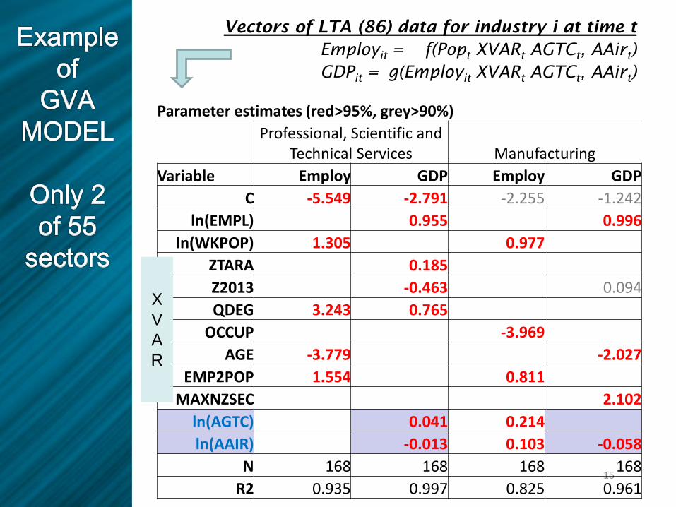
Parameter estimates (red>95%, grey>90%)Professional, Scientific and

Technical Services ManufacturingVariable Employ GDP Employ GDP

C -5.549 -2.791 -2.255 -1.242ln(EMPL) 0.955 0.996

ln(WKPOP) 1.305 0.977ZTARA 0.185Z2013 -0.463 0.094QDEG 3.243 0.765

OCCUP -3.969AGE -3.779 -2.027

EMP2POP 1.554 0.811MAXNZSEC 2.102

ln(AGTC) 0.041 0.214ln(AAIR) -0.013 0.103 -0.058

N 168 168 168 168R2 0.935 0.997 0.825 0.961

XVAR

Vectors of LTA (86) data for industry i at time tEmployit = f(Popt XVARt AGTCt, AAirt)GDPit = g(Employit XVARt AGTCt, AAirt)

ecpc

SCGE Model Zonal Maps

• Auckland, Hamilton, Tauranga and (rest of) Waikato are residential and work zones.

• Ports are only for exports and imports by air or sea.

• Other NZ is a ‘land port’.

ecpc

SCGE Outline (1)

𝑈𝑈𝑘𝑘𝑘𝑘 = 𝑉𝑉𝑘𝑘 + 𝜀𝜀𝑘𝑘𝑘𝑘

𝐿𝐿𝑘𝑘∑𝑘𝑘 𝐿𝐿𝑘𝑘

=𝑒𝑒𝑉𝑉𝑘𝑘

∑𝑘𝑘 𝑒𝑒𝑉𝑉𝑘𝑘

Utility (U) of household j which selects option k (where to live and where to work) is given by:

Here Vk is the general utility attached to live/work option k and εkj is an idiosyncratic element of utility. Utility is gained from consumption of goods and land (location), not from transport.

From the standard multinomial logit model the proportion of households (L) who select option k is given by:

In other words the ratio of the utility of option k to total utility is the equal to the proportion of households who choose that option. So the number of households choosing any given live/work option k is:

𝐿𝐿𝐿𝐿 𝐿𝐿𝑘𝑘 = 𝑐𝑐 + σLn(𝑈𝑈𝑘𝑘)

Households

ecpc

SCGE Outline (2)Production and Trade

Xw = λwLwβ Nw

1−β

Agglomeration effects enter via λ. Output is a composite of transport and other goods:

𝐸𝐸𝑤𝑤𝑤𝑤 = 𝜑𝜑𝑤𝑤𝑤𝑤(𝑃𝑃𝑇𝑇𝐷𝐷𝑤𝑤𝑤𝑤)𝜂𝜂Exports outside the region from work zone w via port zone p:

𝐺𝐺𝑢𝑢𝑢𝑢 = 𝑔𝑔𝑢𝑢𝐿𝐿𝑢𝑢𝐿𝐿𝑣𝑣

(𝐷𝐷𝑢𝑢𝑣𝑣)𝛿𝛿

Goods demand by home zone is converted into demand by work zone or port zone (for imports from outside region) by a gravity model:

𝑋𝑋𝑤𝑤 = 𝜃𝜃𝐺𝐺𝑤𝑤 + 𝑇𝑇𝑤𝑤

ecpc

SCGE Outline (3)

TransportTransport services consumed in each region are equal to the sum of commuting and freight margins (all to households).

𝑇𝑇𝑟𝑟 = �𝑤𝑤

(𝐿𝐿𝑤𝑤𝑟𝑟𝐷𝐷𝑤𝑤𝑟𝑟 + 𝐹𝐹(𝑤𝑤+𝑤𝑤)𝑟𝑟)

Assorted other equations and identities:• Supply-demand balance• Household income and expenditure• Industry costs and revenue• Regional balance of payments and GDP

Model expressed in logarithmic form and solved by matrix inversion(≈ 220x220) using GAUSS.

ecpc

First and second phase resultsWaikato Expressway & Kaimai Ranges

Implicit in the productivity gains is an implied reduced need for employment; -4,500 people or 0.21% fewer.

Where do they go?

Scenario 1: Supply of industrial land is fixed in each zone and the total regional supply of labour is fixed. No agglomeration benefits.

Scenario 2: As in Scenario 1 plus 1% (induced?) extra labour and residential land.

Scenario 3: As in Scenario 2 plus agglomeration benefits.


Agglomeration effect

(from GVA)

Auckland 0.24% 0.01%

Waikato 0.17% 0.31%

Hamilton 0.12% 0.54%

Tauranga 0.18% 0.44%

Mean 0.22% 0.12%

ecpc

Case StudyWaikato Expressway & Kaimai Ranges (3)


Res

iden

tial

zone

Auckland 0.1% 4.4% 9.7% 17.0% 0.2%Waikato 3.1% -0.8% 0.3% 7.9% 0.0%Hamilton 5.2% -0.5% -0.8% 7.3% -0.5%Tauranga 14.2% 6.5% 10.3% -0.7% -0.2%Total 0.2% -0.3% -0.2% -0.3% 0.1%


Res

iden

tial

zone

Auckland 0.2% 9.8% 21.3% 37.4% 0.5%Waikato 6.9% -1.8% 0.8% 17.4% 0.1%Hamilton 11.3% -1.1% -1.7% 16.0% -1.0%Tauranga 31.1% 14.2% 22.6% -1.5% -0.4%Total 0.5% -0.7% -0.5% -0.6% 0.2%

Scenario 1: Changes in utility including commuting and migration by residence and work zone

Scenario 1: Changes in utility excluding commuting and migration by residence and work zone

ecpc

• Still a pilot model.

• Time not explicit.

• Largely Neo-Classical world.

• Aggregation bias (2 industries).

• No lumpiness in production.

SCGE Model Caveats

ecpc

Future Improvements?1. Cobb-Douglas production and consumer utility

functions are limiting.

2. Other (non-transport) goods may be too broad. Could miss benefits of reallocated expenditure.

3. Splitting other goods would also present an opportunity to distinguish between goods of different transport intensity and allow better links to agglomeration benefits.

4. Elasticity values such as σ in need more research.

5. Business time savings are not directly captured in the model – simulated as productivity improvements, but only in relation to transporting freight.

ecpc

Conclusion

• The gains from a spatial reallocation of economic activity outweigh those from greater population density – at least for this particular case study. (Hensher et al, 2012, found a similar relative mix of effects for a proposed rail link in Australia).

– Suggests may get

• Under a scenario of growing labour force over the combined regions, the road improvements are likely to lead to relatively higher population and workforce growth rates in Auckland and relatively lower growth in the other zones.

• In all cases the improvement in household utility is at least as much as the improvement in GDP, the result of people being able to better match their residential location, work location and consumption to their preferences.

• These are gains from greater allocative efficiency; gains that occur even when there is no change in the total level of resources (land and labour) available to the economy.

the economic impacts of connectivity

Documents