1

 

THE EFFECT OF EXCHANGE RATE MOVEMENT ON TRADE BALANCE IN ETHIOPIA

AUTHOR: Borena Dessalegn Lencho Submitted: To Professor Nobuhiro HIWATARI, THE University Of Tokyo, In Fulfillment for: International Political Economy Class.

July, 2013

2

Executive Summary Despite the existence of multiples of theoretical and empirical studies that have examined the

relationship between exchange rate devaluation and trade balance, there are still heated debates

among scholars over the impact of devaluation on trade balance both in developed and

developing countries. Since the significance of our study lies in understanding how changes in

the exchange rate affects the balance of trade in the long run and the short run, we examined the

evaluation of this relationship. Accordingly, in the long run, we found that depreciation succeeds

in improving trade balance deficit of Ethiopia. Similarly, the short run dynamic error correction

model indicated that changes in trade balance in the short run is explained by changes in Real Effective

Exchange rate and by two years lagged changes in same variable. Moreover, Ethiopia’s export is

characterized by high commodity and geographic concentration, by high susceptibility to

external shocks, high dependence on agricultural export that in turn depends on vagaries of

nature, high price and low income elasticity of demand, and low supply response. On the other

hand, imports intrinsically are highly price inelastic which are either necessities in production

or consumption or very strategic commodity and are invariably required by the country.

Therefore, the gap between export-import leads to a persistent deficit trade balance in the

country. Finally, we wrapped up our argument by concluding that the existence of persistent

trade balance deficit is fundamentally structural in nature in Ethiopia, because imports are

essential in nature that they are price inelastic and therefore cannot simply be discouraged or

easily substituted while exports are highly concentrated on agricultural primary commodities

that are very sensitive to whether condition and price shocks.

3

Chapter One

1. Introduction

1.1 Statement of the Problem

The effectiveness of exchange rate depreciation in improving the trade balance has long been an

issue of considerable interest to economists and policy makers. Especially, since the break down

of the Bretton Woods Accord in 1973, and the advent of floating exchange rates, there has been

renewed interest on the effect of devaluation on the trade balance of both developed and

developing countries. The mixed empirical support of the relationship between trade balance and

changes in exchange rate provides the impetus for investigation of the relationship. Developing

countries failing to meet their development plan have lurched from one development paradigm to

another: from industrialization to import substitution, to export promotion, to Structural

Adjustment Program (Rawlins and Praven, 1993).

Structural Adjustment Program (SAP) is a term used by the IMF for the changes it recommends

for developing countries so that they could get loans with certain conditionality. In implementing

one of the essential components(conditions) of the SAP, less developed countries (LDCs) facing

balance of payment problems due to expansionary financial policies, a deterioration in terms of

trade, price distortions, high debt servicing or combination of these factors have often resorted to

devaluing their currencies (Nashashibi, 1983).

Ethiopia, being one of the LDCs, faced various problems including some of the fore mentioned

ones and others which were the root causes of poor economic performance of the 1970s and

1980s. Even though the causes of poor economic performance were numerous and various, poor

macro-economic policies were the prominent ones. Thus, need for comprehensive, compatible,

timely and sequential policy restructuring was indisputable for reliable and sustained growth and

development and for maintenance of both external and internal balance of the country. In order

to do that Ethiopia has undergone various policy and structural reforms both at micro-and macro-

level of the economy in the form of implementing Structural Adjustment Program (SAP), which

4

began in 1992, after the fall of the Derg regime1. As part of these overall reform program, on

October 1, 1992, Ethiopian Birr devalued from its nominal level of 2.07 Birr per US dollar to

5.00 Birr per US dollar depreciation by about 142 percent.

When the Structural Adjustment Program was introduced in October 1992, the nominal

exchange rate of Birr vis-a-vis the US Dollar had been fixed for nearly three decades, except the

revaluation of 1971, 1972, and 1973 with cumulative nominal revaluation of 17 percent. Such a

passive exchange rate policy, coupled with expansive monetary and fiscal policies, led to

continuous overvaluation (Alem, 1996). Despite the fact that the rate was fixed against the dollar

for this period, it was floating against all other major currencies, following the fluctuation of US

dollar against these currencies (Befekadu and Berhanu, 1999/00). After the massive devaluation

of 1992, the Ethiopian Birr has consistently been depreciating in nominal terms from year to year

and by the year 2012/13, the average nominal exchange rate stood at 18.6518 Birr per US dollar

(depreciation of about 274 percent compared to the 1992, 5.0 Birr per USD).

As vividly explained in Reinhart (1995), devaluations have often been used by developing

countries to reduce large external imbalances, correct perceived "overvaluations" of the real

exchange rate, increase international competitiveness, and promote export growth. However,

devaluation can only accomplish these tasks if it translates in to a real devaluation and if trade

flows respond to relative prices in significant and predictable manner. This shows that nominal

devaluation is not a goal in itself.

However, it is discussed in Edwards (1989) that in theory and under most common conditions,

nominal devaluation will affect an economy in three main ways. First, devaluation will usually

have an expenditure reducing effects. To the extent that as a result of devaluation the domestic

price level goes up, there will a negative wealth effect that will reduce the real value of domestic

currency dominated nominal assets, including domestic money. A lower real value of assets will

reduce expenditure on all goods. Second, it will tend to have an expenditure switching effect.

This involves shifts in the pattern of domestic demand from tradable towards non-tradable, and

the pattern of domestic production from non-tradable to tradable. The combined effect of

expenditure reducing and expenditure switching will, of course, improve the external situation of

the country. Third, devaluation will increase the domestic price of imported intermediate inputs 1 Military Junta that governed Ethiopia from 1974 to 1991

5

and imported capital goods. This will increase the cost of production and results in a contraction

of real output or aggregate supply, including non-tradable.

Although economic theory posits that devaluation of a country's currency will likely improve the

trade balance, there are conflicting theories about the effect of devaluation on trade balance.

Empirical findings of Rose (1990), Dhakal D. (1997) both suggested mixed results.

1.2 Objectives of the study

The general objective of this research is to scrutinize the impacts of changes in exchange rate

movement on trade balance, i.e., whether depreciation improves trade balance or not.

More specifically, the study attempts:

To briefly look at exchange rate regimes and developments in Ethiopia

Briefly investigate the structures and trends of import and export situation in Ethiopia.

To empirically investigate the short run and long run impact of change in exchange rate

of Birr on trade balance of Ethiopia

To make conclusions and policy implications

1.3 Definition

An exchange rate is the price of one nation’s currency in terms of another nation’s currency.

Changes in exchange rates are given various names depending on the kind exchange rate regime

prevailing. Under the floating-rate system, a fall in the market price (the exchange rate value) of

a currency is called a depreciation of that currency; a rise is an appreciation. We refer to a

discrete official reduction in the otherwise fixed par value of a currency as devaluation;

revaluation is the antonym describing a discrete rising of the official par (Pugel and Lindert,

2000).

Appreciation/revaluation is a rise in the price of a country's currency in terms of foreign

currency while depreciation/devaluation is a fall in the price of a country's currency in terms of

foreign currency. Devaluation and depreciation are similar: devaluation is generally used for

discrete change in the exchange rate brought about as a matter of policy, whereas depreciation

occurs gradually through the working of the foreign exchange market. Revaluation and

6

appreciation are antonyms for devaluation and depreciation respectively. From these definitions

one can easily understand that devaluation/depreciation means an increase in nominal or real

exchange rate while revaluation/appreciation means decrease in nominal or real exchange rate

regardless of how they come about. Therefore, devaluation and depreciation and also revaluation

and appreciation could often be used interchangeably. In this study, exchange rate is defined as

the units of the home currency per a unit of the foreign currency. Therefore,

depreciation/devaluation is an increase in exchange rate (for instance, increase in Birr/USD ratio)

and appreciation/revaluation is a fall in exchange rate (for instance, decrease in Birr2/USD ratio).

1.4 Significance of the study

To the best of the author’s understanding, there are limited studies that have examined the impact

of changes in the exchange rate on trade balance of Ethiopia. The importance of this paper, thus,

lies in contributing to the existing literature and also in contributing to the definitive

understanding of how changes in the exchange rate affects trade balance that could have vast

implications to the endeavor to improve the country’s competitiveness and to promote export,

and so to formulate good policy that could help improving the persistent trade deficit.

1.5 Data source and methodology of the study

The data source for this study include different annual publications of the National Bank of

Ethiopia, International Financial Statistics (IFS) publications, The IMF and World Bank data

bases, Ethiopian Macro model data base, direction of trade publications and other relevant

sources and covers a period of roughly 38 years. The employed model is believed to be

appropriate and simple to examine the relationship between exchange rate changes and trade

balance. Utmost effort is made to use latest econometric techniques of analysis3.

2 Birr is the name of Ethiopian currency for transaction 3 All the econometrics techniques and procedures followed are explained under chapter 4.

7

1.6 Organization of the Paper

The paper is organized in five chapters. The first chapter presents introductory part of the study.

The second chapter deals with the review of theoretical and empirical literature on the research

topic. The third chapter presents a brief look at the structure of and trends in exports and imports.

The fourth chapter presents the model to be used in the analyses and presents the empirical

results of the study. The last chapter presents conclusion and policy implications.

Chapter Two

2 Review of Theoretical and Empirical Literatures

2.1 Theoretical Literature

2.1.1 The different approaches to the relationship between exchange rate

changes and trade balance

Despite the existence of plethora of theoretical and empirical studies that have examined the

relationship between exchange rate devaluation and trade balance, there are still heated debates

over the impact of devaluation on trade balance both in the case of developed and developing

countries (Ahmad, J. & Yang, J. 2004). Since the significance of our study lies in understanding

how changes in the exchange rate can affect the balance of trade in the long run and the short

run, we need to assess the different approaches in the evaluation of this relationship.

Generally, ever since the failure of the presumption of automatic adjustment of the balance of

payments, three approaches have been developed in investigating the impact of exchange rate

changes on balance of payments. These are the Elasticity approach, the Absorption approach and

the Monetary approach to be discussed in detail below.

8

2.1.1.1 The Elasticity Approach

This approach provides an analysis of what happens to trade balance when a country devalues its

currency and conditions that must prevail in the foreign exchange market for a devaluation or

depreciation of the currency to improve the trade balance starting from equilibrium (Pongsak

Hoontrakul( 1999). According to Sugman (2005), the analysis was developed by Alfred

Marshall, Abba-Lerner and later extended by Joan Robinson (1937) and Fritz Machlup (1955).

At the outset, the model makes some simplifying assumptions. It is partial equilibrium analysis –

holding constant everything else that may affect the supply of and demand for foreign or

domestic currency, except the change in the relative price of foreign and domestic goods arising

from the change in the exchange rate itself. The approach focuses on demand conditions and

assumes the supply elasticities for the domestic export goods and foreign import goods are

infinite, i.e. perfectly elastic so that changes in demand volumes have no effect on prices (the

domestic price of exports, the foreign price of imports and prices of import and export substitutes

are constant). In effect these assumptions mean that domestic and foreign prices are fixed so that

changes in relative prices are caused by changes in the nominal exchange rate.

Under these assumptions, the condition for a devaluation to improve the trade balance which

directly contributes to the improvement of the balance of payments (starting from equilibrium) is

known as the Marshall-Lerner condition. It states that devaluation will improve the balance of

payments on trade balance if the sum of the foreign price elasticity of demand for exports (ηx)

and domestic price elasticity of demand for imports (ηm) exceeds unity, in absolute value, i.e. if:

│ + │ > 1 -------------------------------------------------------------- (2.1)

Consider a small one percent devaluation which leads to a one percent fall in the foreign price of

domestic exports. If the demand for exports rises by less than one percent, foreign exchange

earnings will fall; if demand rises by more than one percent foreign exchange earnings will rise,

and if demand rises by exactly one percent, foreign exchange earnings will remain the same. In

this last case of unitary elasticity of demand, it would then only require a minute cutback in

import demand (an elasticity of demand for imports slightly above zero; > 0) for foreign

exchange earnings to improve in total. Any combination of price elasticity of demand for

9

exports and imports will improve foreign exchange earnings provided that they sum to greater

than unity.

Starting from equilibrium, the improvement in the trade balance (∆TB) is measured as:

dTB= X ( + -1) dE ------------------------------------------------------ (2.2)

where X is the initial level of exports (= imports), and dE is the instantaneous change in the exchange

rate (measured as the domestic price of a unit of foreign currency).

In keeping with Pugel and Lindert (2000), the central message of the elasticity approach is that

there are two direct effects of devaluation on trade balance one which works to reduce and the

other one works to worsen. These two effects are the price effect and the volume effect. The

price effect clearly contributes to the worsening of trade balance because exports become

cheaper measured in foreign currency and imports become expensive measured in the home

currency. The volume effect obviously contributes to the improving of trade balance. This is

because of the fact that exports become cheaper should encourage an increased volume of

exports and the fact that imports become expensive should lead to a decreased volume of

imports. The net effect depends upon whether volume or price effect dominates.

There is a general consensus by most economists that elasticity are lower in the short- run than in

the long -run, in which case Marshal -Lerner condition may only hold in the medium to long-

run. The possibility that in the short run, Marshal-Lerner may not be fulfilled although it

generally holds over the long run leads to the phenomenon of what is popularly known as the J-

curve effect. The idea underlying the J-curve effect is that in the short run export volumes and

import volumes do not change much, so that the price effect outweighs the volume effect leading

to deterioration in trade balance. Three of the most important reasons advanced in explaining the

J-curve effect are time lag both in producers and consumers response and imperfect competition.

Driskell, Robert A. (1981), made a refinement of the elasticity approach by incorporating income

effects into the analysis. According to them, if autonomous money expenditure remains constant,

allowing for income effects does not alter the Marshall-Lerner condition for a successful

devaluation, but the magnitude of the effect on the balance of payments is altered. With this

effect equation (2.2) becomes:

10

dTB = X ( + -1) dE ----------------------------------------------------------------------(2.3)

where s is the propensity to save and m is the propensity to import. Since s/(s + m) is a fraction,

the change in the balance of payments is smaller with income effects than without (becomes less

stringent).

According to same source, a seemingly contrary result was derived by Harberger (1983). His

models hold real expenditure constant implying a rise in autonomous expenditure in money

terms, which suggests that the income effects of devaluation alter the Marshall-Lerner condition,

making it more stringent. According to these models the condition for trade balance

improvement becomes:

│ + │ > 1 + m1 + m2 ---------------------------------------------------------------------------(2.4)

Where m1 is the marginal propensity to import of the devaluing country and m2 is the marginal

propensity to import of the other countries. Which model specification should be preferred

depends on whether a successful devaluation is interpreted to mean one which improves the

balance of payments with real income falling or without real income falling.

Mariana Colacelli (2006) argued that outside of the confines of the partial equilibrium

framework adopted by the elasticity approach, supply elasticity matter both in themselves, and as

determinants of the terms of trade. What happens to expenditure (or absorption) as the terms of

trade change also matters. It can be shown, for example, that if the product of the supply

elasticity of exports and imports exceed the product of the demand elasticity, the terms of trade

will decline, and if expenditure does not fall by as much as real income, the balance of payments

will worsen.

In general, there is highly held view that this approach made very simplistic assumption and it is

by no means certain that in practice the elasticity condition are satisfied, or that, by the time they

are satisfied the competitive advantage gained by depreciation has not been eroded by the

induced price rise.

11

2.1.1.2 The Absorption Approach

Absorption approach due to Alexander (1952) and Johnsen (1967) and popularized by Miles

(1979) was developed to overcome some of the shortcomings of the elasticity approach. The

major purpose of the absorption approach is to integrate the balance of payments with the

functioning of the total economy in a general equilibrium framework, in which balance of

payments disequilibrium on current account is viewed as the outcome of the difference between

decisions to produce and spend, or to save and invest.

Taking the national income identity:

Y = C + I +G+ X – M ------------------------------------------------------------------------------ (2.5)

where C is consumption; I is investment, G is government expenditure, X is exports and M is

imports and defining domestic absorption as A=C + I + G and trade balance as TB= X – M

equation (2.5 ) can be rearranging as:

TB = Y – A ----------------------------------------------------------------------------------------- (2.6)

That is, trade balance is the difference between income (gross domestic product) and absorption.

Alternatively, since Y – C– G is savings (S), equation (2.6) can be rewritten as:

TB = S – I --------------------------------------------------------------------------------------- (2.7)

Similarly, the absorption approach can be spelled out using the leakage -injection terminology

(Hallwood and Macdonald, 2000). Thus, S+T+M=I+X+G and on rearrangement (S-I) + (T-G)

=X-M. Where T is tax and the other variables are as defined above .That is net national saving

equals trade balance. Within this framework, devaluation can be evaluated in terms of whether it

raises income (Y) relative to absorption (A), or saving (S) relative to investment (I). Therefore,

understanding how devaluation affects both income and absorption is central to the absorption

approach. Policies to raise Y are termed expenditure switching policies, and include tariffs,

import quotas, export subsidies and devaluation. Policies to reduce A are termed expenditure

reducing policies and include higher taxes, lower government expenditure, higher interest rates

(Hallwood and Macdonald, 2000 and Thirlwall, 2004). Taking the difference of equation (2.6), we

have:

dTB = dY - dA -------------------------------------------------------------------------------------------- (2.8)

Devaluation will have direct effects on income (dY), direct effects on absorption (dA), and indirect

effects on absorption working through changes in income whose magnitude depends on marginal

12

propensity to absorb, α (determined by the propensity to consume and invest) (α dY). Thus, the

change in total absorption dA is given by:

dA= α dY+dAd ---------------------------------------------------------------------------------------- (2.9)

Substituting (2.8) in equation (2.9):

dTB = dY – (α dY + dĀ) = dY (1 - α) - dĀ --------------- (2.10)

Equation (2.10) reveals that there are three factors to be considered in the analysis of the impact

of devaluation in absorption approach. (i) How does devaluation affect income? (ii) What is the

value of α, the propensity to absorb, and (iii) How does devaluation affect absorption directly?

The Effects of devaluation on national income: There are two direct effects of devaluation on

income. The first is an idle resource (less than full employment) effect and the second is a terms

of trade effect. Employment effect: If there are idle resources and providing the Marshall-Lerner

condition is fulfilled, income will increase depending on the degree to which the rest of the

world absorbs more exports and the value of the income multiplier. It is noteworthy, however,

that even if income increases, the trade balance will only improve if the marginal propensity to

absorb is less than unity i.e., α < 1.

The terms of trade effect: The term of trade is the price of exports over the price imports, which

can algebraically be expressed as:

Price of exports/ Price of imports=P/EP* , where E is nominal exchange rate

Deterioration in terms of trade follows devaluation, because devaluation tends to make imports

more expensive in domestic currency term which is not matched by corresponding rise in export

prices. This deterioration in terms of trade lowers national income, because deterioration in terms

of trade means a loss of real national income, as more units of exports have to be given to obtain

a unit of import. However, Laursen and Metzler (un- dated) noted that the deterioration in terms

of trade following devaluation will have two effects on absorption: the substitution effect and the

income effect. While the deterioration in terms of trade lowers national income and thereby

income related absorption, it also makes domestically produced goods relatively cheaper

compared to foreign produced goods, which implies a substitution effect in favor of increased

consumption of domestically produced goods. If the positive substitution effect outweighs the

negative income effect, Laursen –Metzler (un-dated) noted that a devaluation which results in a

deterioration of terms of trade could actually lead to a rise in absorption.

13

In the elasticity approach, a worsening of the terms of trade will improve the trade balance if the

Marshall-Lerner condition is satisfied. In the absorption approach, it depends on the value of α.

If α < 1, a worsening of the terms of trade which reduces income will worsen the trade balance.

Generally, the effect of devaluation on income of the devaluing country is ambiguous and

depends on the net effects of employment effect and terms of trade effect. If there is full

employment (∆Y = 0) and/or if α > 1 and income expands, devaluation cannot be successful in

improving the balance of payments unless there is a direct fall in absorption (∆Ā < 0).

The Effects of devaluation on direct absorption: There are different possible ways through which

devaluation can be expected to impact upon direct absorption such as the real income effect, the

income redistribution effect, money illusion effect, e.t.c. The real income effect: Given an

unchanged money stock, i.e. the case where the authorities do not alter the level of money supply

to the change in money demand, devaluation tends to raise the over all price index. This rise in

price likely reduces the real value of people’s money holdings. If economic agents try to restore

their real money holdings, this will force economic agents to cut down direct absorption. If,

however, the authorities try to respond to the increased money demand by increasing money

supply, the effects of devaluation on direct absorption will be sterilized.

The income redistribution effect: A rise in general price index resulting from devaluation is

likely to have many effects on income redistribution: from fixed income groups to the rest of the

economy; from wages to profits; from imported input reliant firms to exporting firms; from tax

payers to government. All these effects are plainly exposited in Pilbeam (1998) and Thriwall

(2004). If devaluation /depreciation effects lead to the redistribution of income from those with

low marginal propensity to absorb to those with high marginal propensity to absorb, this will

increase direct absorption. The reverse effect lowers direct absorption

Money illusion: It may likewise reduce real consumption, although perhaps only temporarily

until agents realize that they are spending less in real terms.

Finally, as discussed above the effects of devaluation are many, often conflicting and

indeterminate. It should also be noted that equations (2.9) and (2.10), which portrays the balance

of payments as the difference between income and expenditure, or savings and investment, are

14

derived from the national income identities, and causation must never be inferred from these

identities (Thriwall,2004).

2.1.1.3 The Monetary Approach

The monetary approach to devaluation analysis was pioneered by M.Whitman, K.Frekel and

H.Johnson (Carbaugh, 1995). The fundamental basis of the monetary approach to the balance of

payments is that the balance of payments is a monetary phenomenon and not a real phenomenon.

It is argued that any disequilibrium in the balance of payments is a reflection of disequilibrium in

money markets. Three key assumptions that underlie the monetary model are the stable money

demand function, vertical aggregate supply schedule and purchasing power parity (Pilbeam,

1998).

The elasticity and absorption approaches apply to the trade account of the balance of payments,

neglecting the capital movements. Thus, the essence of the monetary approach to the balance of

payments is that it takes the balance of payments as a whole (the current and capital account) and

assumes that changes in international reserves (as the measure of payments imbalance) are a

function of disequilibrium between the supply of, and demand for, money. An excess supply of

money leads to a loss of international reserves (a deficit), and an excess demand for money leads

to a gain in international reserves (a surplus); and changes in the level of reserves are the

mechanism by which the balance between the supply and demand for money is restored. The

monetary approach argues that currency depreciation can only be successful if it increases the

nominal demand for money relative to the supply, as the price level rises, or by reducing the real

supply of money in relation to the real demand (Thirlwall, 2004). Quoting the same author

"Johnson (1977) once asserted ‘all balance of payments disequilibria are monetary in essence.

So-called “structural” deficits or surpluses simply cannot exist’. The IMF, which is heavily

‘monetarist’ in its thinking, rationalizes devaluation not only in terms of its encouragement to

supply more traded goods, but also within this monetary approach, by devaluation reducing the

real value of the money supply".

The monetary approach emphasizes that a devaluation will a have only a transitory beneficial

effect on the balance of payments only so long as the authorities do not simultaneously engaged

15

in an expansionary open market operation. The theme of the monetary approach is that exchange

rate changes are viewed as incapable of bringing about a lasting change in the balance of

payments. As already mentioned, exchange rate change operates strictly by causing

disequilibrium in the money market, causing a deficit or surplus in the balance of payments

which continues only until equilibrium is restored in the money market via reserve changes.

According to Thirlwall (2004), there are two reasons why the monetary approach to the balance

of payments has died a slow death. The first is that, strictly speaking, the model assumes fixed

exchange rates with changes in the excess supply/demand for money affecting the level of

reserves, whereas since 1972 the world has been on floating rates under which the balance of

payments is supposed to look after itself (at least if the floating is ‘clean’) so that there is no need

for reserves. The supply and demand for money determines the exchange rate and not the

balance of payments. The second, and more important, reason concerns the assumptions on

which the monetary approach is based, which have come to be seen as totally unreal in the

changing and volatile conditions of the world economy over the past few years. The first major

assumption is that deficits can only arise if there is disequilibrium in the money market. This

supposition, as in the absorption approach, is also derived from an identity. In this case, the

identity is Walras’s Law that in a model of only two assets, money and goods, an excess demand

for goods (i.e. a balance of payments deficit) must mean an excess supply of money. Apart from

the confusion between plans to spend and produce and actual spending and production, the

limitations of the model are obvious when it is extended to many assets, with disequilibrium in

the capital market or any other market as the source of disequilibrium, combined with ex ante

equilibrium in the money market. Another major weak assumption is that there is no sterilization

of reserve movements by the monetary authorities through open market operations so that the

money supply always falls as reserves fall, and rises as reserves rise. If there is sterilization of

reserve movements, there cannot be a one-to-one relation between the money supply and reserve

movements.

16

2.2. Empirical Literature

Many empirical analyses, both multi-country panel regressions and econometric models applied

to individual countries, have been conducted to show how exchange rate changes affect the trade

balance of developing and developed countries. Despite these plethoras of theoretical and

empirical researches into how exchange rate changes affect trade balance, there is still

considerable disagreement concerning the relationships between these economic variables and

the effectiveness of currency devaluation as a tool for increasing a country's balance of trade

(Onafowora, 2003).

Existing empirical analyses show mixed results of how exchange rate changes affect the trade

balance. The following empirical works clearly witness these facts as presented in Sugman

(2005) and states that "Amongst 30 countries studied, Rose (1990; 271-3) finds that the impact

of devaluation on trade balance is insignificant for 28 countries, and one country shows negative

impact. He concluded that devaluation does not necessarily lead to an increase in trade balance.

Upadhyaya and Dhakal (1997; 343-5) also suggested that improvement in trade balance is only

found in one country out of eight countries studied. On the other hand, others like Bahmani-

Oskooe (1998; 89-96) and Himarios (1989; 143-68) found trade balance improvement following

currency devaluation."

Damoense and Agbola (2004) came with evidence that supports the view that devaluation of

exchange rate worsens trade balance. In their study of the impact of devaluation on trade balance

of South Africa, they found that in the long run, devaluation of exchange rate worsens trade

balance. Similarly, the empirical study by Agbola (2004), by using the Johansen multivariate co-

integration procedure and the Stock-Watson dynamic Ordinary Least Square model (DOLS),

revealed that devaluation did not improve the trade balance of Ghana. Contrary to this, Sugman's

(2005) finding of the effects of real exchange rate depreciation on the real trade balance of

Indonesia divulges improvement in trade balance following depreciation.

The study by Rawlins and Praveen (2000), examined the impact of devaluation on trade balance

of a sample of 19 countries in Sub-Saharan Africa by specifying and estimating an Almon

Distributed lag process of trade balance using annual data. They found in no case did real

17

exchange rates revert to their pre-devaluation levels and in seventeen of nineteen countries real

exchange rate depreciation did improve a country's trade balance in the year of the devaluation.

Onafowora (2003), also examined the short run and long run effects of real exchange rate

changes on the real trade balance of three Asian countries in their bilateral trade with Japan and

USA and found improvement in their trade balance but with time lag. In the case of Ethiopia, the

study by Equar (1999) showed that real exchange rate depreciation improves trade balance.

However, the study by Equar has not included very important explanatory variables (due to

unavailability of the data) that could have radical change on the results obtained and this paper

included some of these variables.

Generally, these mixed results clearly indicate that both empirical and theoretical studies could

not definitely put the relationship between exchange rate changes and trade balance. This

unresolved issue necessitated me to understand the impact of exchange rate changes on trade

balance in Ethiopia where there is persistent trade deficit.

Chapter Three

3. A Snapshot of Ethiopian Exchange Rate Regimes and Developments and

Overview of the Structure and Trends of Exports and Imports of Ethiopia

3.1 Exchange Rate Regimes and Developments in Ethiopia

Our world has experienced different exchange rate regimes and experimented with various types

of exchange rate arrangements within each ever since the emergence of the international Gold

Standard by 1870 to the emergence of the floating rate of 1973. It is clearly indicated in Pugel and

Lindert (2000) that the success or the failure of these different exchange rate regimes depends

historically on the severity of the shocks with which those systems have had to cope with.

When come to history of exchange rate regimes in Ethiopia, the country experienced only two

major exchange rate regimes. These are the pre-1992 fixed exchange rate regime where the

Ethiopian Birr was pegged to the USD and the post -1992 managed -floating exchange rate

regimes. After the birth of IMF and also after the issuance of Ethiopian legal currency, Ethiopia,

18

as one of the founding members, committed itself to the Articles of Agreement of IMF under

which each currency assigned a central parity against USD and was allowed to fluctuate by minus

or plus 1 percent of this parity. Countries were allowed to devalue or revalue their currencies only

in case of 'fundamental disequilibria' (Felleke, 1994).

Ethiopian legal tender currency was issued on 23 July 1945, by defining the monetary unit as the

Ethiopian dollar (E$) with a value of 5.52 grains (equivalent to 0.355745 grams) of fine gold and

replaced the Maria Theresa which had been circulating as legal tender. The linkage with fine gold

was in accord with the monetary system established by the Bretton Woods Agreement of 1944 and

it automatically established the exchange rate between the national currency and other currencies

with the same arrangement. Accordingly, the official exchange rate of Ethiopian currency with US

dollar was created (with the official exchange rate of 2.48 Birr per US dollar) on July 23, 1945.

After almost two decades, that is, on 1 January1964, the Ethiopian Birr was slightly devalued to

2.50 Birr per US dollar. Following the collapse of the Bretton Woods System in 1971 and the

floating of dollar and ceasing of its convertibility to gold, the Birr was revalued to 2.30 Birr per

US dollar (i.e. by 8.75%) on 21 December1971. The subsequent 10% devaluation of the US dollar

had temporarily brought about under valuation of the Birr. To realign the Ethiopian Birr, it was

again revalued to 2.07 Birr per US dollar in February 1973. This fixed official exchange rate was

left unaltered for two decades despite the floating of the major world currencies including the US

dollar (Befekadu, 1991; Derrese, 2001).

According to Haile Kibret (1994), Asmerom Kidane (1994), Equar Dasta (2001), Alem Abraha

(1996)), as a result of fixation of exchange rate, Birr became over-valued in terms of the US dollar

as well as many other foreign currencies. This overvaluation had adverse effect on national

economy such as misallocation of resources, loss of international competitiveness, development of

illicit parallel market for foreign exchange and illicit cross border trade.

Cognizant of these facts, the massive devaluation of 1992 took place. Following this devaluation,

in an attempt to liberalize foreign exchange market, the National Bank has taken a number of

initiatives. Accordingly, the fortnightly auction market for foreign exchange was introduced on

May 1, 1993 with two rates, namely the Dutch auction system (official rate) and marginal pricing

auction system (marginal rate). These two rates were unified in July 1995. In August 1996, the

19

fortnightly auction market was changed to weekly to accommodate the growing demand for

foreign exchange and commercial banks were allowed to also established foreign exchange

Bureaus. In September1998, the retail auction system was replaced by wholesale system .In the

same year, the inter- bank foreign exchange market was introduced and worked alongside the

auction system until October 25,2001 when the daily inter-bank has fully replaced wholesale

auction system (Deresse, 2001). In the present day, the official exchange rate is determined in the

daily inter-bank foreign exchange market as the weighted average exchange rate prevailing on the

preceding day.

3.2 The Structure and Trends of Exports and Imports of Ethiopia

In the following discussions, the major components of export and import and their performances

over the period 1980/81 to 2010/11 will be briefly assessed. That is, the performance of the

components will be evaluated on their average values for the periods of 1980s, 1990s and last ten

years (2000/01-2010/11).

Just to begin with, it becomes common language that Ethiopia's external trade is characterized by

highly sectoral and commodity concentration (high agricultural and single commodity (coffee)

dependence -no commodity diversification on export side, and high capital and consumer

concentration on import side) and also by high geographical concentration (to and from a

particular destination and origin -no market diversification). There has been a widely held view

that such commodity and geographic concentrations are the major causes for the instability in

Less Developed Countries' export earnings to which Ethiopia is not exceptional. This would

make a country's economy vulnerable to external shocks. Factors such as bad weather conditions,

production or marketing problems, and international price shocks affecting one or two of these

commodities can cause a huge swing in export volumes, values, or both. This undoubtedly urges

diversification of both commodities and markets. It is known fact that, Ethiopia's export is dominated by only a few numbers of agricultural

commodities such as coffee, hides and skins, chat, pulses, live animals and oilseeds. In the 1980s

seven items (coffee, petroleum and petroleum products, hides and skins, chat, pulses, live

animals and oilseeds in the order of their decreasing share of total export) have on average

20

accounted for about more than 90% of all exports. For long time, there has been heavy reliance

of export performance on coffee which on average accounted for USD 252 million 63%, USD

234 million 57% and USD 217.2 million 38.1% of export in 1980s, 1990s and over the last ten

years respectively (Table 3.1).

21

Source: National Bank of Ethiopia and own computation n.a = not available **The revised GDP at market price of the 2005/06 constant producers' price has been used.

When we look at the contribution of coffee export to GDP, it accounted for an average of 4% of GDP

in 1980s and 1990s and 3% of GDP during the last ten years. This shows the fact that the share of

coffee and non-coffee in the total export has been decreasing and increasing respectively partly due

to decline in earnings from coffee exports and partly due to an increase in the non-coffee exports.

Chat recently became quite important and is now the second largest export after coffee, over taking

hides and skins in 1998/99 and accounting on average for about USD 71 million 13% of exports

during the last ten years. The shares of other commodities such as oilseeds, pulses and live animals

have also been gradually increasing. Other commodities such as flower, fruits and vegetables, meat

and meat products and spices are among the products which have been recording a considerable

increase in the value of export. This signifies the endeavor of the country to end the single

Table (3.1): Average Value of Export Earnings by Major Commodity Groups

Period 1980/81-1984/85

1985/86-1989/90

1990/91-1994/95

1995/96-1999/00

2000/01-2004/05

2005/06-2010/11

Coffee 247.07 256.99 149.80 318.21 214.00 220.42 Oil Seeds 10.31 5.69 3.58 26.26 59.22 61.00 Hides & Skins 44.21 59.74 39.88 44.87 58.24 59.99 Pulses 11.68 8.65 6.01 12.81 23.94 24.66 Meat & Meat Products 3.06 1.70 0.34 3.63 5.52 5.69 Fruits & Vegetables 2.21 4.22 2.73 5.16 10.65 10.97 Sugar 4.51 8.24 2.95 0.77 9.40 9.68 Live Animals 6.61 9.78 1.22 1.18 3.25 3.35 Chat 12.14 8.45 14.80 46.62 71.26 73.40 Petrol. & Pet. Products 32.72 14.75 11.41 4.81 0.00 0.00 Gold n.a n.a 27.44 25.99 41.34 42.58 Others 22.92 21.04 14.51 26.71 66.77 68.77 Grand Total 397.43 399.26 274.67 517.00 563.58 580.49 % Coffee in total export 62.14 63.81 53.41 61.41 37.57 38.70 Coffee in GDP** 4.58 3.57 2.41 4.98 2.90 2.99 Export in GDP** 7.36 5.52 4.34 8.08 7.70 7.93

22

commodity dominance and it is a decent outcome that indicates an effort in market and commodity

diversification.

Towards the end of 1980s and the beginning of 1990s export performance was getting worse and

worse and by 1991/92, both coffee USD 81 million and export USD 154 million attained their lowest

for the period under observation. Following the 1992 devaluation both coffee and total export

showed a remarkable improvement. Even if there is an improvement, according to report on

Ethiopian economy by Ethiopian Economic Association 2011/12, the overall performance of export

sector has been weak for the past four decades as evidenced by low export/GDP ratio and the

declining share of exports in financing imports which has led to compression of essential goods and

to the rise of debt burden.

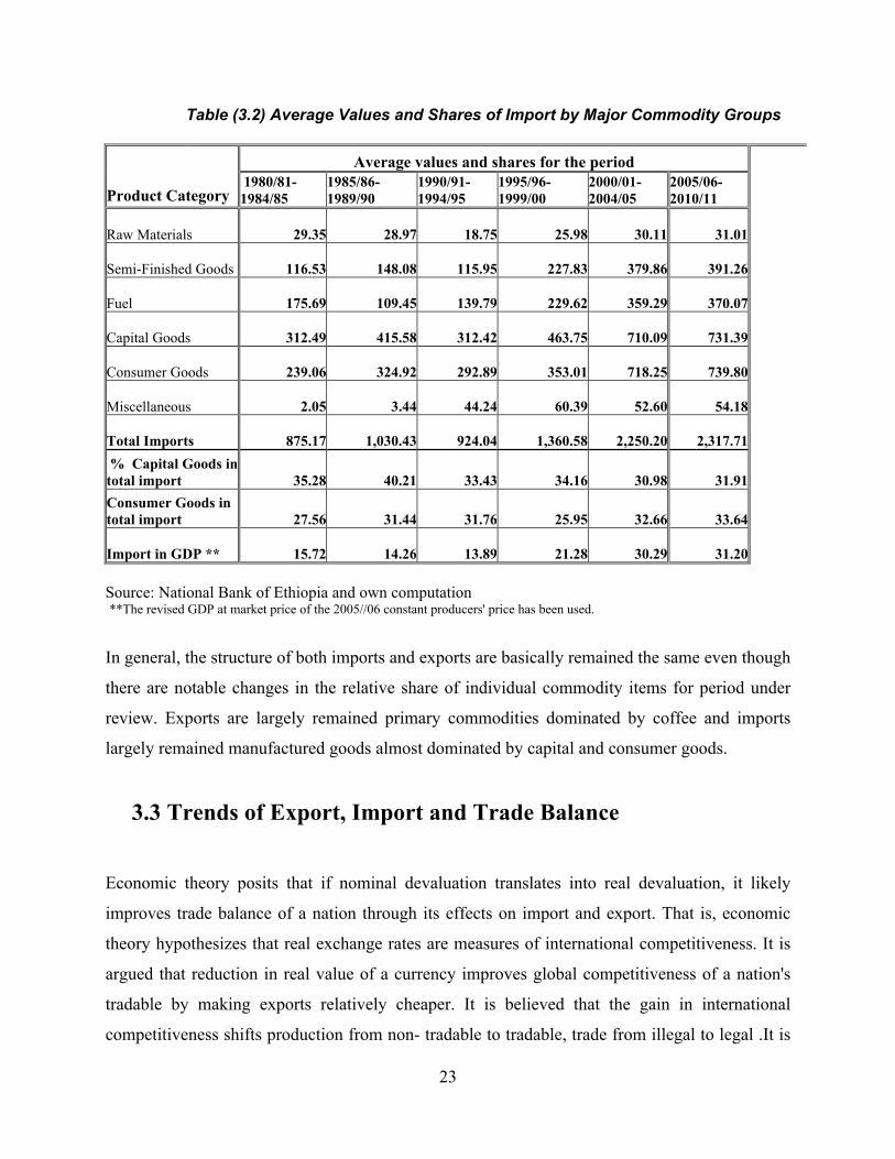
When we come to the structure of imports, it essentially remained the same for the period under

consideration. In 1980s, 1990s and the last ten years, capital goods and consumer goods together

contributed for an average of more than 63% of total import which indicates heavy reliance on

imported capital and consumer goods. It can be observed from (Table 3.2) that on average the shares

of raw materials and capital goods are falling while that of consumer goods and semi finished goods

are rising and that of fuel is more or less remained constant. The share of import in GDP has

consistently been increasing ever since 1991/92.

23

Table (3.2) Average Values and Shares of Import by Major Commodity Groups

Average values and shares for the period

Product Category 1980/81-1984/85

1985/86-1989/90

1990/91-1994/95

1995/96-1999/00

2000/01-2004/05

2005/06-2010/11

Raw Materials

29.35

28.97

18.75

25.98

30.11 31.01

Semi-Finished Goods

116.53

148.08

115.95

227.83

379.86 391.26

Fuel

175.69

109.45

139.79

229.62

359.29 370.07

Capital Goods

312.49

415.58

312.42

463.75

710.09 731.39

Consumer Goods

239.06

324.92

292.89

353.01

718.25 739.80

Miscellaneous

2.05

3.44

44.24

60.39

52.60 54.18

Total Imports

875.17

1,030.43

924.04

1,360.58

2,250.20 2,317.71 % Capital Goods in total import

35.28

40.21

33.43

34.16

30.98 31.91

Consumer Goods in total import

27.56

31.44

31.76

25.95

32.66 33.64

Import in GDP **

15.72

14.26

13.89

21.28

30.29 31.20 Source: National Bank of Ethiopia and own computation **The revised GDP at market price of the 2005//06 constant producers' price has been used.

In general, the structure of both imports and exports are basically remained the same even though

there are notable changes in the relative share of individual commodity items for period under

review. Exports are largely remained primary commodities dominated by coffee and imports

largely remained manufactured goods almost dominated by capital and consumer goods.

3.3 Trends of Export, Import and Trade Balance

Economic theory posits that if nominal devaluation translates into real devaluation, it likely

improves trade balance of a nation through its effects on import and export. That is, economic

theory hypothesizes that real exchange rates are measures of international competitiveness. It is

argued that reduction in real value of a currency improves global competitiveness of a nation's

tradable by making exports relatively cheaper. It is believed that the gain in international

competitiveness shifts production from non- tradable to tradable, trade from illegal to legal .It is

24

also argued that devaluation makes import expensive and hence discourages it. The combined

effect of increased competitiveness and discouraged imports is expected to improve trade

balance. In this study, we examine whether Ethiopia's experience substantiate this theory.

To see the applicability of this theory we examine the impact of the changes in real exchange

rate with Ethiopia's major trading partners on export and import and consequently on trade

balance. According to our definition, an increase in real effective exchange rate (REER) implies

depreciation, which likely enhances the international competitiveness of the country, given the

relative price kept constant. The REER index with other indices is plotted in figure (3.1) below.

The figure shows movements in nominal exchange rate index (NERI) with USD, real exchange

rate index (RERI) with USD, nominal effective exchange rate index (NEERI), and real effective

exchange rate index (REERI)4.

Observation of the trend of real effective exchange rate index from 1970/71 through 2010/11,

reveals about seven distinctive periods with few exceptions: depreciation from 1970/71 through

1974/75, appreciation from 1975/76 through 1985/86 but 1978/79 and1980/81, depreciation in

1986/87and 1987/88, appreciation from 1988/89 through 1991/92, depreciation by about 64 % in

1992/93 and kept through 1995/96, appreciation in 1996/97 and 1997/98 and depreciation

continued thereafter but the year 2002/03 and 2003/04. Examining export, import and trade

balance for the corresponding periods indicates discrepancy between theory and experience for

most of the period of observation.

4 The data for these indices are obtained from exchange rate database of the National Bank of Ethiopia.

25

For instance, contrary to the theory, the depreciation of the REERI for 1995/96, 2000/01-2010/12

could not have helped the improvement of the competitiveness of Ethiopia’s exports in the

international market. However, the scrutiny of the data from Annual Report of National Bank of

Ethiopia, explicates a big jump in export value in Birr from 279 million in 1991/92 to 800 million

(187 percent) in 1992/93. In line with the theory, export increased for three consecutive years

following the massive devaluation and subsequent depreciation of REER. However, for most of the

period under consideration, export did not improve or deteriorate following depreciation or

appreciation of REER respectively, showing the indecisive relationship between changes in exchange

rate and export value and therefore trade balance.

It is also observed that import was not discouraged by depreciation of REER. Opposite to the theory, it

had invariably been increasing regardless of whether the REER had depreciated or appreciated for most

of these distinctive periods. For instance, despite the depreciation of REER from 1992/93 through

1995/96 import was steadily growing.

 -­‐          20.00      40.00      60.00      80.00    

 100.00      120.00      140.00      160.00      180.00    

1970/71  

1972/73  

1974/75  

1976/77  

1978/79  

1980/81  

1982/83  

1984/85  

1986/87  

1988/89  

1990/91  

1992/93  

1994/95  

1996/97  

1998/99  

2000/01  

2002/03  

2004/05  

2006/07  

2008/09  

2010/11  

Exchan

ge  Rate  Inde

x  Figure 3.1: Movements in Nominal and Real Exchange Rates

Source: the National Bank of Ethiopia

NEERI  REERI  RERI  NERI  

Period  

26

Figure (3.2) indicates the steady growth of both export and import following the 1992

devaluation. The growth rate of import was relatively lower from1992/93 through 1995/96. From

1996/97 through 2010/11, import grew at high rate while export grew slowly; the growth of the

former exceeds that of the latter. Although both export and import grew, the trade deficit has

been widening because the base for import growth is relatively larger than the export growth.

 (40,000.00)  

 (30,000.00)  

 (20,000.00)  

 (10,000.00)  

 -­‐        

 10,000.00    

 20,000.00    

 30,000.00    

 40,000.00    

 50,000.00    

1970/71  

1972/73  

1974/75  

1976/77  

1978/79  

1980/81  

1982/83  

1984/85  

1986/87  

1988/89  

1990/91  

1992/93  

1994/95  

1996/97  

1998/99  

2000/01  

2002/03  

2004/05  

2006/07  

2008/09  

2010/11  

Value  in  m

illions  of  B

irr  

Figure 3.2: Trends of Import,Export and Trade balance Source : the National Bank of Ethiopia

M  

X  

X-­‐M  

           period  

27

As elucidated by Figure (3.3), while export as percentage of GDP has been increasing, since

1992/93, it failed to match the faster increase in import and as a consequence the trade deficit as

percentage of GDP has been increasing. Thus, trade deficit both in absolute term and as a

percentage of GDP has been increasing persistently (Figures 3.2 &3.3).

Finally, there is a general consensus that Ethiopia's export is characterized by high commodity

and geographic concentration, by high susceptibility to external shocks, high dependence on

agricultural export that in turn depends on vagaries of nature, high price and low income

elasticity of demand, and low supply response. On the other hand, imports intrinsically are

highly price inelastic which are either necessities in production or consumption or very strategic

commodity and are invariably required by the country. From this very nature of export and

import, it is unlikely to expect the neo-classical theory to apply to Ethiopia. However, these mere

trend analysis and theoretical justification do not suffice. We cannot be conclusive and thus,

substantiation of these facts by empirical examination is necessitated.

 (10.00)  

 -­‐        

 10.00    

 20.00    

 30.00    

 40.00    

 50.00    

 60.00    

Percen

tage  

Figure 3.3 :Trends of imports ,exports and trade balance as a percentage of GDP

Source : the National Bank of Ethiopia

Import  as  Percentage  of  GDP  

Export  as  Percentage  of  GDP  

Trade  Deficit  as  Percentage  of  GDP  

Period  

28

Chapter Four

4. Model Specification and Estimation of Results

4.1 Model Specification

Remembering that, the central point of our investigation is analyzing the impact of changes in

exchange rate on trade balance in Ethiopia. Doing that entails specification of trade balance.

Both theoretical and empirical literatures propose a number of key variables that have significant

effects on export and import and hence on trade balance. Trade balance is usually measured as

the difference between receipts for exports of goods and expenditure for imports of a nation

during a specific period of time. Based on the works of Agbola (2004), Rawlins and Praveen

(2000) and Sugman (2005) trade balance can be specified as:

TB=X - M=X ( , Y*)- M (Pm.E, Y) --------------------------------------------------------------- (4.1)

Where: TB is the trade Balance, X is export earning, M is import payment, Px is the domestic

price of exports, Pm is foreign price of imports, E is Birr per unit of foreign currency, Y* and Y

are foreign and domestic incomes respectively.

Even though trade balance is usually measured as the difference between total value of exports

and total value of imports, in this study, trade balance (TB) is represented by the ratio of exports

to imports. This ratio, or its inverse, has been used in many empirical investigations of trade

balance-exchange rate relationship as referred in Onafowora (2003) and Rincon (1998).

According to them, the use of this ratio has several advantages. First, it is invariant to units as

one measures exports and imports, in other words, whether they are in real or nominal terms or

in domestic or foreign currency, it is invariant. Second, the regression equation can be expressed

in log linear form or constant elasticity form which gives the Marshall-Lerner condition exactly

rather than as approximation and the estimated coefficients is elasticity.

Incorporating monetary policy and fiscal policy variables that affect trade balance into equation

(4.1) in line with economic theory and recent empirical investigation of whether changes in

29

exchange rate improve the trade balance, this study uses a log-linear form and regresses trade

balance over a number of explanatory variables.

Ln(TB)= + Ln(REERI)+ Ln(RGDP)+ Ln(MS)+ Ln(TOT)+ Ln(RWGDP)

+ Ln(RGE)+ (DDRT) + (DPC) +Ui -------------------------------------------------------------------------------(4.2)

Where Ln is natural logarithm, TB is trade balance in Ethiopia, RGDP is real gross domestic

product a proxy for real domestic national income, DDRT is dummy drought or lack of rainfall

that takes the value of one for the years of drought zero otherwise, MS is domestic money

supply, RWGDP is real world gross domestic product a proxy for real income of Ethiopia's

major trading partners, RGE is real government expenditure, TOT is external terms of trade,

REERI is real effective exchange rate index, DPC is dummy policy change which takes value

zero (0) for the period pre 1992/93 reform and one (1) for the period then after, and Ui is the

random error term.

Although the model is thought to capture the effects of the exchange rate on the trade balance in

a model that puts together the elasticity, absorption, and monetary approaches to the balance of

payments, because of unavailability of data, some explanatory variables are not included.

What follows is to look into the theoretical expected impacts of the respective explanatory

variables on trade balance.

REER (+) in our study, the real effective exchange rate is defined as the units of the home

currency per a unit of the foreign currency taken accounts of trade partner countries' trade weight

and relative inflation, depreciation (an increase in REER) is expected to improve the trade

balance. The exchange rate with the trading partners (real effective exchange rate) index is taken

because it is this exchange rate that is usually taken as measure of competitiveness.

RGDP (-) the impact of the real income variable on trade balance is ambiguous. The expected

signs under the absorption and monetary approaches are a negative and positive respectively

with some bold assumptions as already discussed in literature part. Higher income levels

stimulate increased import demand as well as increased domestic production of tradable, leaving

the ultimate impact on the trade balance somewhat indeterminate. However, it is argued that the

former effect dominates the latter.

RWGDP (+?) The impact of an increase in real world income as a proxy for real income of

Ethiopia's major trading partners is ambiguous as discussed above which makes the

30

determination of the sign difficult. Even though it is with uncertainty, the sign expected is

positive as it is argued that increase in income of the trading partners increase the demand for

exports.

RGE (-) It is customarily assumed that any increase in domestic government expenditure that

fails to displace an equal amount of private expenditure will increase total spending (absorption)

thus worsening the trade balance. Here too, there is some ambiguity as the increase in

government expenditure might be complementary to some investment initiative, thus resulting in

a larger output of tradable goods. Nevertheless, it is often assumed with some degree of

uncertainty that the sign on the coefficient of RGE is negative.

MS (-) Even though there is difference on the rationale between schools of thought, they agree in

principle that the signs on domestic money supply should be negative. According to the

Monetarist view, increases in the money supply propel real balances above levels considered

optional by economic agents, resulting in increased expenditure out of a given income thus

stimulating imports and causing the trade balance to deteriorate. For Keynesians, increases in the

money supply reduce interest rates thus stimulating increased absorption which puts negative

pressure on the trade balance.

TOT (+) Defined as the relative price of exports to imports, deterioration in terms of trade has

two effects on domestic absorption (hence trade balance): the income effect and the substitution

effect and the net effect depends on the relative strengths of these two effects. However, it seems

that there is a dominant view that deterioration in terms of trade lowers national income, because

deterioration in terms of trade means a loss of real national income, as more units of exports have

to be given to obtain a unit of import. Hence, the effect of the terms of trade on trade balance is

expected to be positive with some ambiguity.

DDRT (-) Ethiopian exports are highly dominated by agricultural commodities which in turn

highly dependent on the availability of rainfall for Ethiopian agriculture is almost exclusively

rain-fed. It intuitively goes that the presence of drought worsens trade balance either by

decreasing export supply and/or by increasing import as relief aid.

DPC (+) Competitiveness policies and supply side reforms which include liberalization,

financial sector reforms that initiates export trade financing and investment, tax reforms, and

others that promotes export development are expected to improve export performance. In spite of

the fact that these policy changes improve imports too, it is expected to improve trade balance by

increasing export supply by more than import demand.

31

The Unit Root and Cointegration Tests The reason for knowing whether a variable has a unit root (that is, whether the variable is

nonstationary) is to avoid the problem of spurious regression-case where the results of regression

suggest that there are statistically significant long run relationship among the variables in the

regression model when in fact all that obtained is being evidence of contemporaneous correlation

rather than momentous causal relation. Stationarity, in language of the time series, means that

mean, variance and autocovariance (at various lags) remain the same no matter at what time

point they are measured; they are time invariant (Gujarati, 2003). Hence, the time series

properties of the data series employed in the estimation of the equation is tested. The presence of

unit roots (non-stationarity) for each variable is tested using the Augmented Dickey-Fuller

(ADF) test procedure and the result of this test is presented on table 4.1. It is shown that all the

variables individually contain a unit root at level, that is, the unit root hypothesis cannot be

rejected at a 5 percent significance level. But, all the variables become stationary in the first

difference i.e. they are I (1). The optimal lag length is determined by using the Akaike

Information criterion.

Conditional up on this outcome of the test for the stationarity properties of the data series, tests

for co- integration of the variables is conducted, because, co-integration necessitates that all

variables of a model to be integrated of the same order. A test for co-integration means looking

for stable long run or equilibrium relationships among non-stationary economic variable. It is

pointed out in Gujarati (2003) that a linear combination of two or more non-stationary series may

be stationary. If such a stationary, or I (0), linear combination exists, the non-stationary (with a

unit root), time series are said to be co-integrated. Therefore, co-integration test is designed to

check for the existence of co-integrating relationships between non-stationary variables. Just

testing the stationarity of the residual term makes test for the presence of co-integration. If the

variables are stationary at level, that is, I (0), they are said to be integrated. Therefore, the test is

undertaken by using Augmented Dickey-Fuller (ADF) test and the result is presented in table

(4.1) below. It shows that the variables are stationary at level.

32

Table (4.1): Result of unit root test for residual series

ADF Test Statistic

Optimum lag

Critical Values -6.420168 1 1%* -3.6496

5% -2.9558 10% -2.6164

*MacKinnon critical values for rejection of null hypothesis of a unit root.

As shown in the table, the null hypothesis that there is unit root is rejected even at 1 percent

significance level witnessing the existence of long run or equilibrium relationship among

economic variables presented in equation (4.2).

33

4.2 Estimation and Interpretation of Results

4.2.1 Long run Results

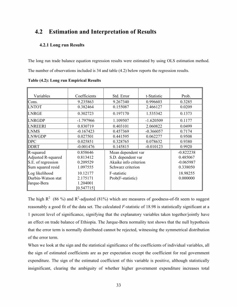
The long run trade balance equation regression results were estimated by using OLS estimation method.

The number of observations included is 34 and table (4.2) below reports the regression results.

Table (4.2): Long run Empirical Results

The high R2 (86 %) and R2-adjusted (81%) which are measures of goodness-of-fit seem to suggest

reasonably a good fit of the data set. The calculated F-statistic of 18.98 is statistically significant at a

1 percent level of significance, signifying that the explanatory variables taken together/jointly have

an effect on trade balance of Ethiopia. The Jarque-Bera normality test shows that the null hypothesis

that the error term is normally distributed cannot be rejected, witnessing the symmetrical distribution

of the error term.

When we look at the sign and the statistical significance of the coefficients of individual variables, all

the sign of estimated coefficients are as per expectation except the coefficient for real government

expenditure. The sign of the estimated coefficient of this variable is positive, although statistically

insignificant, clearing the ambiguity of whether higher government expenditure increases total

Variables

Coefficients

Std. Error

t-Statistic

Prob.

Cons. 9.235863 9.267340 0.996603 0.3285 LNTOT 0.382464 0.155087 2.466127 0.0209 LNRGE 0.302723 0.197170 1.535342 0.1373 LNRGDP -1.797966 1.109507 -1.620509 0.1177 LNREERI 0.830719 0.403101 2.060822 0.0499 LNMS -0.167423 0.457369 -0.366057 0.7174 LNWGDP 0.027501 0.441595 0.062277 0.9508 DPC 0.025851 0.328765 0.078632 0.9380 DDRT -0.001476 0.145815 -0.010123 0.9920 R-squared 0.858646 Mean dependent var -0.822238 Adjusted R-squared 0.813412 S.D. dependent var 0.485067 S.E. of regression 0.209529 Akaike info criterion -0.065987 Sum squared resid 1.097555 Schwarz criterion 0.338050 Log likelihood 10.12177 F-statistic 18.98255 Durbin-Watson stat 2.175171 Prob(F-statistic) 0.000000 Jarque-Bera 1.204001

[0.547715]

34

spending (absorption) thus worsening the trade balance or complement some investment initiative,

thus resulting in a larger output of tradable goods improving trade balance.

The coefficient of the real domestic income variable, RGDP, is negative as expected but statistically

non-significant at a 10 percent level implying that the real domestic income has no statistically

significant effect on trade balance. The positive and statistically significant at a 5 percent level of the

coefficient of the terms of trade variable indicates that improvement in terms of trade ceteris paribus

improves trade balance of Ethiopia. The coefficient of the term of trade variable, which measures the

elasticity of term of trade with trade balance, indicates that improvement in terms of trade by about

10 percent would result in about 3.8 percent increase in trade balance per annum.

Coming to the central objective of this study, that is to investigate the impact of change in exchange

rate on trade balance of Ethiopia, the coefficient of the real exchange rate variable, REERI, is

positive and statistically significant at a 5 percent level confirming the hypothesis that real

depreciation succeeds in improving trade balance of Ethiopia in the long run. The elasticity of real

effective exchange rate 0.83 indicates that depreciation of real effective exchange rate by 10 percent

would result in about 8.3 percent increase in trade balance per year.

The coefficient of the domestic money supply variable is negative but statistically insignificant and is

consistent with the argument that an increase in domestic money supply would lead to an increase in

the level of real balances. This implies that the increase or decrease in domestic money supply does

not have an effect on trade balance of Ethiopia and using this policy solely to influence trade balance

is likely ineffective. The positive coefficient on the real world income variable is positive and

statistically insignificant at 95 percent level of significance .The result indicates that ,ceteris paribus ,

improvements in the income of Ethiopia's trading partners does not bring improvements in trade

balance of Ethiopia in the long run. This result supports the view that exports of developing countries

have low-income elasticity and also consistent with the hypothesis that exports from developing

countries are supply rather than demand determined (Athukorala and Riedel, 1996, Sugman, 2005).

Even though it is statistically insignificant, the dummy policy change has the expected positive

coefficient verifying the fact that the economic liberalization improves trade balance. As expected,

dummy for drought has negative but statistically insignificant coefficient implying that the recurrent

drought has no long run effect on trade balance.

35

Generally, the result obtained shows that real exchange rate depreciation succeeds in improving trade

balance of Ethiopia in the long run which is in line with the finding of Equar (1999). However, the

sign on coefficient of terms of trade is opposite to the one obtained here.

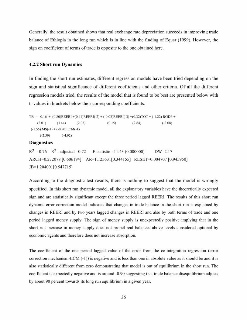
4.2.2 Short run Dynamics

In finding the short run estimates, different regression models have been tried depending on the

sign and statistical significance of different coefficients and other criteria. Of all the different

regression models tried, the results of the model that is found to be best are presented below with

t -values in brackets below their corresponding coefficients.

TB = 0.16 + (0.80)REERI +(0.41)REERI(-2) + (-0.03)REERI(-3) +(0.32)TOT + (-1.22) RGDP +

(2.01) (3.44) (2.08) (0.15) (2.64) (-2.08)

(-1.55) MS(-1) + (-0.90)ECM(-1)

(-2.59) (-4.92)

Diagnostics

R2 =0.76 R2 adjusted =0.72 F-statistic =11.43 (0.000000) DW=2.17

ARCH=0.272078 [0.606194] AR=1.125631[0.344155] RESET=0.004707 [0.945950]

JB=1.204001[0.547715]

According to the diagnostic test results, there is nothing to suggest that the model is wrongly

specified. In this short run dynamic model, all the explanatory variables have the theoretically expected

sign and are statistically significant except the three period lagged REERI. The results of this short run

dynamic error correction model indicates that changes in trade balance in the short run is explained by

changes in REERI and by two years lagged changes in REERI and also by both terms of trade and one

period lagged money supply. The sign of money supply is unexpectedly positive implying that in the

short run increase in money supply does not propel real balances above levels considered optional by

economic agents and therefore does not increase absorption.

The coefficient of the one period lagged value of the error from the co-integration regression (error

correction mechanism-ECM (-1)) is negative and is less than one in absolute value as it should be and it is

also statistically different from zero demonstrating that model is out of equilibrium in the short run. The

coefficient is expectedly negative and is around -0.90 suggesting that trade balance disequilibrium adjusts

by about 90 percent towards its long run equilibrium in a given year.

36

Chapter Five

5.1 Conclusion, policy implication and Recommendation

The objective of this paper has been to examine the short-and long-run effects of real exchange

rate changes on trade balance of Ethiopia which adds to the understanding of the relationship

between the two. It is also hoped that the finding of this paper would provide useful information

in an effort to limit trade balance deficit. Accordingly, the paper has examined empirically the

role of exchange rate changes in determining the short-and long-run behavior of the Ethiopian

trade balance under a model that nets the elasticity, absorption, and monetary approaches to the

balance of payments. Devaluation or depreciation of exchange rate is expected to improve the

international competitiveness of the devaluing or depreciating country by changing the relative

price of home and foreign goods. There are different approaches with different transmission

mechanisms in assessing the impact of these changes in exchange rate on trade balance. An

utmost effort has been made to observe these different approaches to the balance of payments.

An attempt was also made to briefly see exchange rate regimes and development in Ethiopia. In

the third chapter, it is also attempted to assess the structure and trends of exports and imports and

it is found that the structure of export basically remains the same with some slight changes.

There are high sectoral (primary agricultural commodities), commodity (coffee) and market

concentration indicating the high vulnerability of the country's export to both supply and demand

side shocks. The structure of import also basically remains the same during period under

observation and it is also highly commodity and market concentrated. The close scrutiny of

export and import performance corresponding to distinctive periods of real effective exchange

rate changes shows mixed result which makes determination of the relationship between

exchange rate changes and trade balance an empirical issue.

In addressing the central point of investigation, a simple model is specified and estimated. After

specification of the model, the time series properties of the data are investigated. Doing that

entails unit root test and co-integration test. The unit root test by using the Augmented Dickey-

Fuller (ADF) test procedure has shown that the variables are non-stationary at level, but

stationary at first difference; they are I (1). The co-integration test shows that the variables are

co-integrated, and therefore share a long-run relationship.

37

The long run trade balance equation regression results were estimated by using OLS estimation

method and empirical results indicate that, in the long run, there is positive relationship between

the real exchange rate depreciation and trade balance. The policy implication of this finding is that

real exchange rate depreciation can improve the international competitiveness of the country thereby

improving its trade balance deficit and consequently the balance of payment deficit in the long run.

The coefficient of the domestic money supply variable is negative but statistically insignificant and

this implies that the increase or decrease in domestic money supply does not have an effect on trade

balance of Ethiopia and using this policy exclusively to influence trade balance is ineffective. The

exhibited positive and statistically significant coefficient of the term of trade variable indicates that

improvement in terms of trade, ceteris paribus, improves trade balance of Ethiopia.

The short run dynamic analysis revealed that, trade balance in the short run is explained by

changes in REERI and by two years lagged changes in REERI and also by both terms of trade

and one period lagged money supply.

Generally, the existence of persistent trade balance deficit is fundamentally structural in nature

because Ethiopia's imports are essential/necessity in nature that they are price inelastic and

therefore cannot simply be discouraged or easily substituted while exports are highly

concentrated on agricultural primary commodities that are very sensitive to whether condition

and price shocks.

Recommendations

Based on the empirical findings and the general structure of exports and imports as components of trade

balance the following policy recommendations are forwarded to help improve the persistent trade deficit.

Firstly, since the empirical results obtained indicate the existence of long run relationship between real

exchange rate changes and trade balance, to make and keep Ethiopia competitive, keeping the

track of international exchange rate adjustment is crucial.

Secondly, as a complimentary policy instrument to real exchange rate depreciation, compatible policies

such as tight monetary and fiscal policies should be implemented (maintained if they prevail) timely and

38

sequentially to avoid the possible depletion of the competitive advantage obtained by real exchange rate

depreciation due to rise in domestic prices.

Thirdly, since the persistent trade deficit, is basically structural in nature, other supplementary

policy options to real exchange rate depreciation are deemed necessary to curb the problem. These

are:

a) On export side h Diversification of export commodities through identification of new comparative advantages and

development of new export products, improving the quality of the existing export products, increasing

the productivity of export producers by training and providing price incentives

b) On import side

h Production of quality substitutes should be encouraged and awareness creation in favor of the home

Produced substitutes should be made to help cut the large import bill

References

39

1. Ahmad, J. & Yang, J. (2004), Estimation of the J-curve in China: Economics Series East West center working papers. 2. Alem, 1996), ‘‘Exchange Rate Systems in Ethiopia, Published by Mega Printing Enterprise, Addis Ababa, Ethiopia.” 3. Alem Abraha(1995), “Export Performance of Ethiopian Economy.” 4. Alexander,s.s,(1952), Effects of A Devaluation on Trade Balance, International Monetary Fund Staff Papers,2,pp. 263-278. 5. Bahmani- Oskooe (1998; 89-96) and Himarios (1989; 143-68), Nominal and Real Effective Exchange Rates of Middle Eastern Countries and their Trade Performance, Applied Economics,33 pp.103-111. 6. ( Befekadu and Berhanu, 1999/00), ‘Trade Balance and Changes in Exchange rate in Ethiopia: Birr vs Baskets of Currencies’ Birritu Megazine volume 103, Addis Ababa, Ethiopia. 7. Bafikadu(1991) “Exchange rate regimes in Ethiopia.” 8. Damoense and Agbola (2004), The J-Curve: Evidence from Fiji*. Authors: Paresh Kumar Narayan1; Seema Narayan1. Source: International Review of Applied Economics, Volume 18. 9. Deresse Degefa(2001), “Export Performance And Economic Growth In Ethiopia.” 10. Driskell, Robert A. 1981. Exchange rate dynamics: An empirical investigation, Journal of Political Economy 89. 11. Edwards (1989), Real Exchange Rates, Devaluation and Adjustment: Exchange Rate Policies in Developing Countries, Cambridge, Mass: MIT Press. 12. Equar (1999), Determinants of Trade Balance in Ethiopia. 13. Felleke (1994), “Export Performance and Economic Growth in Ethiopia.” 14. Haile Kibret,Asmarom Kidane, (1994), “Exchange rate regimes and Export sub sector Development in Ethiopia.” 15. Hallwood, Paul, and Ronald MacDonald (2000), International Money and Finance, 3rd ed. (paper back), Oxford and Cambridge. 16. Harberger (February 1983)-Laursen-Metzler Effect, " Journal of Political Economy ,volume 91 . " 17. Johnsen (1967), Johnson, Harry G. 1958. Towards a general theory of the balance of pay ment, In International trade and economic growth, ed. H. G. Johnson. London: Allen & Unwin Miles (1997), The J-curve revisited: an empirical examination for the United States, Journal of International Money and Finance.

40

18. Laursen and Metzler (undated), Flexible Exchange Rates and The Theory of Employment. 19. Mariana Colacelli (2006). “Export Responses to Exchange Rate Fluctuations: An Empirical Analysis”. 20. M.Whitman, K.Frekel and H.Johnson (Carbaugh, 1995), The monetary approach to devaluation analysis. 21. Nashashibi, (1983), Do Devaluations Improve the Trade Balance? The Evidence Revisited. 22. Onafowora, O. (2003). Exchange rate and trade balance in East Asia: Is there a J-curve. Economic Bulletin, Vol. 5, No.18, pp. 1-13. 23. Pongsak Hoontrakul( 1999), “Review of Exchange Rate Theory.” 24. Pugel and Lindert (2000), International Economics, Irwin Professional Publishing, 1996, 10th Edition. 25. Rawlins and Praveen (2000), Effects of Exchange Rate Volatility and changes in Macroeconomic Fundamentals on Economic Growth in Ghana. 26. (Rawlins and Praven, 1993), Devaluation and the Trade Balance: The Recent Experience of Selected African Countries. 27. Reinhart (1995), Devaluation, Relative Prices, and International Trade: Evidence from Developing Countries , Staff Papers - International Monetary Fund Vol. 42, No. 2 (Jun., 1995), pp. 290-312. 28. Rose (1990), ‘Exchange Rates and the Trade Balance: Some Evidence from Developing Countries’, Economics Letters, 34(3), November, pp. 271-75. 29. Sugman (2005), “Combined effects of exchange rate movement on export.” 30. Sugema, I. (2005), The determinants of trade balance and adjustment to the crisis in Indonesia: Centre for international economics studies, No.0508. 31. Thirlwall (2004), Trade Liberalization and Economic Performance in Developing Countries, The Economic Journal. 32. Upadhyaya, K.P. and Dhakal, D. (1997) , ‘Devaluation and the Trade Balance: Estimating the Long Run Effect’, Applied Economics Letters, 4(6), June, pp.343-45, the Long Run Effect’, Applied Economics Letters, 4(6), June, pp.343-45.