Thelek

The effect of pretrial detention on labor market outcomes

Autores:

Nicolás Grau Gonzalo Marivil

Jorge Rivera

Santiago, Mayo de 2021

SDT 518

The effect of pretrial detention on labormarket outcomes∗

Nicolas Grau† Gonzalo Marivil‡ Jorge Rivera§

May 29, 2021

Abstract

We combine Chilean individual administrative data for criminal cases and labormarket outcomes to estimate the effect of pretrial detention on labor outcomesusing the Difference-in-differences (DiD) method and an instrumental variables(IV) approach. The IV approach takes advantage of the quasi-random assignmentof judges. The IV results show that pretrial detention reduces the probability ofhaving formal employment and the average monthly wage by 39% and 56% duringthe six months following the final trial verdict. DiD estimation delivers estimatesthat are between one-third and one-half smaller. The magnitudes of the effectsshown continue to be relevant as much as 24 months after the final trial verdict.The results of our analysis suggest that the negative effect of pretrial detention is(at least) driven by the lasting effect of being excluded from the labor market duringthe trial, the accompanying social stigma, and the impact of pretrial detention onthe probability of post-verdict incarceration.

Keywords. Wages and unemployment, Criminal Law, Pretrial detention, Incar-ceration.

∗We thank the Chilean Public Defender’s Office (Defensorıa Penal Publica), the Chilean Ministry of Labor and theDirector of Studies office of the Supreme Court (Centro de estudios de la Corte de Suprema) for providing the data. Wethank Diego Amador, Nadia Campaniello, Dante Contreras, Alejandro Corvalan, Patricio Domınguez, Felipe Gonzalez,Jeanne Lafortune, kevin Lang, Francisco Pino, Juan Wlasiuk and seminar participants at the Workshop on Prison con-ditions, labor markets, and recidivism (University of Bologna, Department of Economics, 2016), LACEA–LAMES 2018(Ecuador), Sechi 2018, Econ department of the Universidad Diego Portales, Law department of the Universidad de Chile,Law department of the Universidad Diego Portales, for helpful comments and suggestions. Nicolas Grau thanks the Cen-tre for Social Conflict and Cohesion Studies (ANID/FONDAP/15130009) for financial support. Powered@NLHPC: Thisresearch was partially supported by the supercomputing infrastructure of the NLHPC (ECM-02).

†Department of Economics, Faculty of economics and business, University of Chile (Santiago). ngrau@fen.uchile.cl.Corresponding author.

‡Central Bank of of Chile (Santiago). gmarivil@fen.uchile.cl§Department of Economics, Faculty of economics and business, University of Chile (Santiago). jrivera@econ.uchile.cl

1

1 Introduction

At a global level, around one-third of individuals charged with a crime (approximately

2.8 million) are subject to “pretrial detention” (see Walmsley (2016)), a judicial measure

to incarcerate accused individuals after they have been arrested and charged until their

trail as a precautionary measure or to protect the investigation. Advocates of pretrial

detention usually justify this measure based on the concern that the accused will not

appear in court, may be a danger to others, or may interfere with the investigation.

Detractors hold that pretrial detention is not only a threat to the presumption of in-

nocence, a keystone of all contemporary judicial systems,1 but could also have moral,

social, and economic costs for the accused, including an impact on their posttrial labor

market outcomes.2

In Chile, the focus of this study, individuals detained pretrial as percentage of the total

prison population rose from 21.9% in 2007 to 36% in 2017. The corollary of this trend has

been an increase in the number of individuals detained pretrial but who were either found

not guilty or whose punishment did not include a custodial sentence. Furthermore, the

time accused individuals who are detained pretrial spend in prison is not insignificant:

16.1% spent less than ten days in prison, 49.7% spent between ten days and six months,

and 34.2% were incarcerated for more than six months.3

To assess the potential impacts of pretrial detention, this paper evaluates its effect

on post-verdict labor market outcomes using Chilean data.4 We use a novel dataset that

merges individual administrative data on pretrial detention and labor market outcomes

for arrested occurred between 2008 and 2016. The pretrial detention data comes from

the Public Defender’s Office records and the labor market outcome data comes from

the administrative records from the Chilean unemployment insurance office. The labor

market outcome data covers employment and wages and includes the monthly individual

labor performance for all people who work in the formal private sector.

1See Article N◦ 11 of the United Nation’s Universal Declaration of Human Rights.2See Open Society Fundations (2011) and Open Society Fundations (2014).3All statistics on pretrial detention are from the Public Defender’s Office (Defensorıa Penal Publica,

DPP), the Chilean public institution that provides free legal representation for almost all individualsaccused in criminal cases.

4For general perspective on mas incarceration and labor market see Weiman et al. (2007) and Western(2007).

2

To obtain causal estimates in this context is challenging. The pretrial detention de-

cision is made by a judge who is likely to observe individual characteristics that we, as

econometricians, can only partially observe. Moreover, these characteristics are probably

correlated with labor outcomes. We follow two empirical strategies to address this endo-

geneity problem. First, and since the Chilean setting is characterized by a quasi-random

assignment of judges for arraignment hearings at the court-by-time level, we build and

use a measure of judge severity as an instrument to estimate a two-stage least squares

(2SLS) model, following Dobbie et al. (2018) and Dahl et al. (2014). An important fac-

tor for the efficacy of this instrument is that the judges that preside over arraignment

hearings determine pretrial detention but not final verdicts. We show suggestive evi-

dence that this instrument meets the conditions of independence, relevance, exclusion,

and monotonicity (Imbens and Angrist (1994)). Second, we take advantage of a panel

database that begins several months before the person is arrested and ends after the

final trial verdict to estimate a panel data DiD model, controlling for individual fixed

effects. For reasons that are discussed in the paper, our preferred specification is the

2SLS model.

By estimating the IV and DiD models, we show a short-term (i.e., between one and

six months after treatment) negative impact of pretrial detention on the probability of

having a formal job that is between 9.8 (IV) and 17.8 (DiD) percentage points (pp).

This equates to a reduction of 21% and 39%. With respect to average monthly wages,

the negative short-term effect is −32, 227 and −92, 635 Chilean pesos (CLP) for the DiD

and the IV estimations, or about 50 and 150 US dollars (USD). These point estimates

represent a decrease of 20% and 56.7% in an individual’s average monthly wage. These

results are robust to alternative specifications. Regarding the persistence of these effects,

there is a reduction in the point estimates in the case of employment over time, but the

trend is less clear for wages. That said the negative effect of pretrial detention on both

employment rate and average monthly wages is still relevant 18 to 24 months after

treatment.

Using the DiD model we study two dimensions of treatment heterogeneity. First, we

show that the negative effects are much larger for those who were detained pretrial for

longer 5 by dividing the treatment group into terciles based on the time they spent in

5This result is contrary to the findings in Kling (2006) and Landersø (2015), but it is more in linewith Ramakers et al. (2014).

3

pretrial detention. For the short-term effect on employment probability, the effects for

the first, second, and third terciles are −4.5, −8.5, and −16.5 pp; for the short-term

effect on average monthly wage, the effects are −17, 686 CLP (26 USD), −26, 810 CLP

(39 USD), and −52, 900 CLP (78 USD). Second, we estimate the causal effect of pretrial

detention on labor outcomes for those accused individuals who were not incarcerated as

a result of their final trial verdict. We find that the magnitude of the point estimates for

this group is between one-third and one-half lower relative to the full estimation sample.

Regarding mechanisms, we discuss the relevance of three broad explanations for our

results. The first potential explanation considers the importance of the fact that being

detained pretrial removes the accused from the labor market, which may have lasting

consequences on post-verdict employment and wages. This could happen, for example,

because individuals are fired during pretrial detention and post-verdict they have prob-

lems in finding a new job. We refer to this explanation as the labor market hypothesis.

The second explanation examines whether or not pretrial detention carries with it addi-

tional and specific impacts on labor outcomes beyond simply being unable to work during

the detention period. We call this explanation as the social stigma hypothesis : in the

hiring process previously incarcerated people are discriminated.6 Finally, we investigate

whether the effect of pretrial detention on the post-verdict labor market is due to its

positive effect on the probability of post-verdict incarceration. We call this explanation

the labor incapacitation hypothesis. Our results suggest that all these mechanisms may

play a role in explaining the impact of pretrial detention on labor outcomes.

This paper contributes to the literature in two main ways. To the best of our knowl-

edge, it is one of the first papers that estimates a causal effect of pretrial detention

on labor outcomes, and certainly the first using data from a developing country, where

prison conditions tend to be worse.7 Given that we find an effect even for individuals

whose final verdict does not include a custodial sentence, across both guilty and not

guilty verdicts, our findings contrast with the results shown in Harding et al. (2018),

who find an effect of prison sentences on employment but mainly as a result of incapac-

itation. Additionally, by taking advantage of our rich labor market data, we shed some

6On how incarceration and a criminal history can generate a stigma in the labor market see Bushway(2004); Finlay (2009); Mesters et al. (2016), Pager (2003), and Pettit and Lyons (2007). A completediscussion on these two mechanisms can be found in Apel and Sweeten (2014).

7Other papers have used data from a developing country to estimate the effect of pretrial detentionon recidivism, they include Cortes et al. (2019) and Ferraz and Ribeiro (2019).

4

light on the mechanisms that could be causing the effect of pretrial detention on labor

outcomes.

Our paper is related to the growing body of literature that studies the impact of (pre

and posttrial) imprisonment on labor market outcomes. This literature has produced

mixed results. There are studies that find a negative effect of incarceration on labor

outcomes (see Mueller-Smith (2015); Raphael (2007); Western (2006) and Western et al.

(2001)) and other studies have shown that the negative effects could be moderate in

magnitude and rather short-lived (see Grogger (1995)). Some studies, such as Jung

(2011), Lalonde and Cho (2008), Nagin and Waldfogel (1995), and Bhuller et al. (2020)

have shown positive effects for incarceration. For example, Bhuller et al. (2020) uses data

from Norway to show that posttrial discourages further criminal behavior, which is driven

by individuals who were not working prior to incarceration. For them, incarceration

increased future employment and earnings. Their findings demonstrate that time spent

in prison could potentially be pro human capital accumulation for individuals already

having issues with the labor market when incarceration focuses on rehabilitation.

Similar research has been carried out by Dobbie et al. (2018), showing that pretrial

detention decreases formal sector employment, using data that links over 420,000 criminal

defendants from two large, urban counties in the US with administrative court and tax

records. The empirical strategy used in Dobbie et al. (2018), as in this paper, exploits

exogenous variation in pretrial release given the quasi-random assignment of cases to

bail judges.8 They find that pretrial detention decreases the probability of employment

in the formal labor market three to four years after the bail hearing by 9.4 pp (a 24.9%

decrease). This result is smaller than the result from our IV estimations (about half of

our point estimates), if we consider the first 24 months. The larger point estimates in

our setting can be explained by the differences in prison conditions and in labor markets

between the two settings, which reinforces the relevance of studying these policies in

developing countries.

The rest of the paper proceeds as follows: Section 2 briefly describes the Chilean legal

system and the conditions under which pretrial detention is imposed. Section 3 describes

the data and presents some stylized facts on labor market outcomes for treatment and

8This source of exogenous variation has also been used in Aizer and Doyle (2015); Cortes et al.(2019); Dahl et al. (2014); Di Tella and Schargrodsky (2013); Ferraz and Ribeiro (2019); Green andWinik (2010); Knepper (2018) and Kling (2006).

5

the control groups that motivate our empirical strategy in Section 4. Section 5 presents

our findings on the impact of pretrial detention on the probability of being employed

and average monthly wages. Section 6 discusses the possible mechanisms that explain

our results. Finally, Section 7 concludes.

2 Pretrial Detention in Chile

The reform of the criminal justice system in Chile was a gradual process that began

in 2000 and was finalized in 2005. This broad reform, which included a new criminal

code, replaced the inquisitorial model, a written system that had been in place for

more than a century, with an oral, public, and adversarial procedure.9 As part of the

reform, new institutions were created, including the Office of the Public Prosecutor

(Ministerio Publico); the Public Defender’s Office (Defensorıa Penal Publica, DPP); the

Guarantee Court (Juzgados de Garantıa), where hearings that decide pretrial detention

are undertaken; and the Oral Criminal Trial courts (Tribunales Orales de Juicio Penal).

The DPP provides free legal representation for nearly all individuals who have been

accused of committing a crime (more than 95%) and records all defendants that use

their services, including detailed information on the particular crime in question.

In this new system the criminal process has the following stages. The first stage con-

cerns the arrest of the individual, either because they are caught by the police in flagrante

delicto (i.e., the commission of the crime) or as the result of an investigation conducted

by the Public Prosecutor that culminates in an accusation. This stage concludes with an

arraignment hearing at the Guarantee Court, where the detention judge chooses between

three possible outcomes: to begin a criminal proceeding; an alternative ending (which

may include compensation agreements and the conditional suspension of proceedings);

or to simply dismiss the proceedings. It should be noted that most cases are resolved in

the Guarantee Court, either by an alternative ending or dismissal. Generally speaking,

a criminal proceeding is reserved for severe imputed crimes, which are the focus of this

paper.

When the detention judge decides to begin a criminal proceeding, the length of the

trial (considering the time required for an investigation) and any precautionary measures

9See Blanco et al. (2004) for a detailed description of this reform.

6

must be stipulated. Pretrial detention is the most severe precautionary measure and it

must be requested by the prosecutor. The defendant’s attorney is given the opportunity

to advocate for their client with regard to the decision. To support the request for

pretrial detention, the prosecutor may offer the following legal arguments: that the

defendant presents a clear flight risk; that the defendant represents a danger to society;

or the imprisonment of the defendant will aid with the investigation (see Riego and Duce

(2011)). In theory, the prosecutor must put forward a very strong argument for pretrial

detention. Unlike the legal system in the US, defendants in Chile do not have the option

of posting bail in order to avoid pretrial detention.

There are several outcomes for a trial, ranging from a not guilty verdict to a convic-

tion and prison sentence. One characteristic of criminal proceedings in Chile, which is

particularly relevant to our study, is that the pretrial detention decision is kept separate

from other trial outcomes through the use of the two different courts. It is also notable

that the judge that presides over the arraignment hearing does not participate in the

oral proceedings court trial, which is presided over by three separate judges.

Respect for a defendant’s human rights was one of the principal motivations for crimi-

nal justice system reform in Chile. As time has passed, however, this original motivation

has been somewhat forgotten (see Riego and Duce (2011)). Figure 1 illustrates this,

showing that decisions to detain defendants pretrial became more frequent between 2007

(17,891 cases) and 2018 (34,815 cases), which means the proportion of the total cases

that include a pretrial detention has increased from 7.3% to 9.6%. To look at it from

another angle, the percentage of pretrial detainees in relation to the total prison popula-

tion rose from 21.9% in 2007 to 36% in 2017, an increase of 64.4%. Figure 1 also shows

that the number of individuals who were detained pretrial but who were either found not

guilty or whose punishment did not include a prison sentence at all has also increased.

Although, following the literature, we study the impact of pretrial detention on labor

outcomes regardless of trial outcome, we also show the effect for those individuals who

were accused of a crime and detained pretrial but who were not sentenced to prison after

the trail itself.

In sum, although the reformed criminal justice system, implemented between 2000

and 2005, is based on principle of the presumption of innocence, Chile still detains many

individuals who have yet to be found guilty, a trend that has been increasing over time.

7

Figure 1: Evolution of Pretrial Detention

17891

23280 23555

2649428490

3375334815

6942

9543 980611310

12474

16185 17055

1397 1714 1810 2482 2873 3403 3833

010

000

2000

030

000

4000

0

Pre

tria

l Det

entio

ns

2006 2008 2010 2012 2014 2016 2018

Year

All Non guilty + Noncustodial sanctionsNon guilty

Notes: This figure shows the evolution of pretrial detention from 2007 to 2018, using DPP administrative records. Thedynamic is shown for three groups: a) All: considers the full sample; b) Not guilty + non-custodial sentence: includes allthe individuals whose final verdict resulted in no prison time; c) Not guilty: includes those individuals whose final verdictdeclared them not guilty.

Finally, and this is formally tested in the empirical strategy section, it is relevant to

stress that the assignment of arraignment judges does not depend on the characteristics

of the prosecuted individual or the criminal case. Arraignment judges are allocated

across days and cases depending on their workloads. Hence, conditional on court and

year, the assignment of arraignment judges can be considered random.

3 Data and Stylized Facts

3.1 Data

We assemble an administrative, individual-level dataset from the national unemployment

insurance scheme (operated by the Ministry of Labor) and the Public Defender’s Office

(DPP). As previously described, the DPP provides free legal representation for nearly all

individuals who have been accused of committing a crime. For individuals who are not

8

legally represented by a DPP attorney (i.e., those who hired a private attorney), we have

data on their alleged crime but not on the final verdict of their trial. Therefore, given

our treatment and control group definition, we do not include these cases in our sample.

That said, less than 5% of prosecuted individuals are represented by a private attorney

without DPP participation. In this paper, we use the DPP’s prosecution records between

2006 and 2016.

The information provided by the DPP is very detailed on the crime (i.e., the specific

type of crime that we group into broader categories), the court, the time spent in jail

during the prosecution (if any), and the final verdict. Using the final verdict, we can

determine whether the prosecuted individual was found guilty (as well as the punishment)

or not guilty. In addition, the Research Department at Chile’s Supreme Court provided

us with data on all the arraignment judge who presided over arraignment hearings to

decide pretrial detention between 2008 and 2017. This information is useful for our

empirical strategy because it gives us exogenous variation in the probability of being

subject to pretrial detention.

Our labor market data comes from administrative records held by Chile’s national

unemployment insurance scheme. As described in Acevedo et al. (2010), the country’s

unemployment insurance covers all enrolled workers over 18 years who are employed in

private sector salaried jobs. Temporary workers are also included in the system, but

individuals who have been unemployed or working in the public or informal sector since

the unemployment insurance scheme began in 2002, are excluded.10 Participation in the

unemployment insurance scheme is compulsory for all workers who started a new job after

October 2002; it is voluntary for those workers who were already in formal employment

at that time. Therefore, full implementation of this scheme was only achieved after 2005

as workers were gradually incorporated. The database provides monthly data on wages,

type of contract (either full or part time), as well as data on the employer including size

of the firm (measured by the number of workers), economic sector, and a specific firm

ID. The firm ID is useful because it allows us to see if a given worker keeps the same job

over time or switches between jobs. As will become clear in Section 6, the possibility of

keeping a job held pretrial is an important mechanism to explain the effect of pretrial

detention on labor market outcomes.

10We have to exclude 27% of the accused individuals given that for them we do not observe any laborinformation before arrest.

9

Because of data availability issues, we focus on individuals whose prosecutions started

after 2007. And we only consider first-time offenders (as revealed by the DPP data)

because some prosecuted individuals who are not first-time offenders may have low pre-

treatment labor outcomes as a result of their pretreatment imprisonment. We further

restrict the study to those accused of severe crimes -that is, crimes for which more than

10% of cases receive pretrial detention (this restriction is relaxed in the robustness check

analysis).11 Finally, our sample is restricted to those individuals employed for at least

one month in the formal sector during the two years before the beginning of their pros-

ecution: individuals who have no formal work experience would not have contributed to

the unemployment insurance scheme from which we draw our data.

Accordingly, the treatment group are those who were subject to pretrial detention

and the control group are those who were not. Individuals in both the treatment and

the control group were prosecuted for the first time for a severe crime (i.e. a crime for

which in more than 10% of cases the defendant is detained pretrial).

To illustrate the impact of these sample restrictions, Table 1 shows the differences

in a set of variables between the non-restricted sample and the estimation sample. We

do not compare the two groups using the labor market information because most of the

differences between them are due to the lack of labor market information for individual

excluded from the estimation sample. Looking at Table 1 we can observe that the

estimation sample has a greater proportion of men, that individuals in this sample are

more likely to have been charged with more severe crimes, and, consequently, that they

are more likely to be subject to pretrial detention. Additionally, the trials of these

individuals tend to be longer. Of course, a tendency for accusation of a more severe

crime and a higher chance of pretrial detention for individuals in the estimation sample

is deliberate.

To provide a clearer picture of our estimation sample, Table 2 shows the descriptive

statistics for the covariates, reporting the information for the control and treatment

groups separately. A few elements deserve comment. First, individuals in the treatment

group are more likely to be male, and more likely to be of indigenous decent. Second,

individuals in the treatment group are accused of more severe crimes and their trials

11Plea-bargaining is restricted in Chile to minor crimes. Because those crimes have a very low prob-ability of pretrial detention, they are not considered in our estimation sample.

10

Table 1: Estimation sample versus population

Variable All Est. Sample Norm. Dif. p-value

Male 0.79 0.91 -0.358 0.000Indigenous 0.02 0.01 0.023 0.000non-Chilean citizen 0.01 0.01 0.047 0.000Severe crimes 0.07 0.27 -0.553 0.000Pretrial detention 0.02 0.16 -0.479 0.000Days in judicial process 100 190 -0.428 0.000Days in pretrial detention 151 147 0.027 0.002

Observations 1,188,482 142,679

Notes: In this table, the first column (All) considers all the individuals in the DPP database(between 2007 and 2016) who are 18 years or older. The second column (Est. Sample) considersthe sample used in our main estimations. In order to build this sample, we add the followingconditions to the sample restrictions that were made to obtain column (1): (a) individuals musthave been employed for at least one month in the formal sector during the twenty-four monthsbefore the beginning of the prosecution; and (b) individuals must have been accused of crimeswhere pretrial detention is an distinct possibility (i.e., severe crimes, for which in more than10% of cases the defendant is detained pretrial. Norm. Dif. denotes the normalized differencesin the means.

last longer. Third, individuals in the control group tend to have longer labor contracts

although there are no differences in terms of firm size or industry. It is also notable that,

even though our control and treatment groups are very different, none of our empirical

strategies require them to be equal. We examine this point in more detail in Section 4 .

11

Table 2: Summary statistics for the covariates by treatment status

Treated Control

Mean S.d Mean S.d

Demographic variables

Male 0.9393 0.2388 0.9096 0.2868

non-Chilean citizen 0.0086 0.0921 0.0050 0.0703

Indigenous 0.0211 0.1438 0.0127 0.1122

Judicial variables

Severe crimes 0.5473 0.4978 0.2160 0.4115

Days in judicial process 254 222 178 229

Type of contract

Indefinite term 0.3183 0.0011 0.4242 0.0008

Fixed term 0.6817 0.0015 0.5758 0.0010

Firm size

Micro 0.1235 0.0010 0.1398 0.0007

Small 0.2356 0.0016 0.2237 0.0009

Medium 0.2242 0.0018 0.2148 0.0007

Big 0.4167 0.0013 0.4217 0.0011

Firm sector

Agriculture - Silviculture - Industrial Fishing 0.1017 0.0021 0.0921 0.0010

Mining 0.0094 0.0035 0.0117 0.0015

Manufacturing 0.0935 0.0011 0.1045 0.0008

Electricity-Gas-Water 0.0022 0.0076 0.0024 0.0029

Construction 0.3016 0.0012 0.2457 0.0010

Commerce 0.1181 0.0022 0.1367 0.0007

Services 0.2966 0.0014 0.3174 0.0010

Transportation-Communication 0.0730 0.0017 0.0852 0.0009

No information 0.0039 0.0073 0.0044 0.0017

Observations 22,433 120,246

Notes: This table reports the summary statistics for the covariates considered in our esti-mated models, comparing control and treatment groups. The table considers the estimationsample – namely, individuals in the DPP database (between 2007 and 2016) who are 18 yearsor older; who have been employed for at least one month in the formal sector during thetwo years before the beginning of prosecution; and who have been accused of crimes wherepretrial detention is an distinct possibility (i.e., severe crimes, for which in more than 10%of cases the defendant is detained pretrial). S.d denotes standard errors.

12

3.2 Stylized Facts

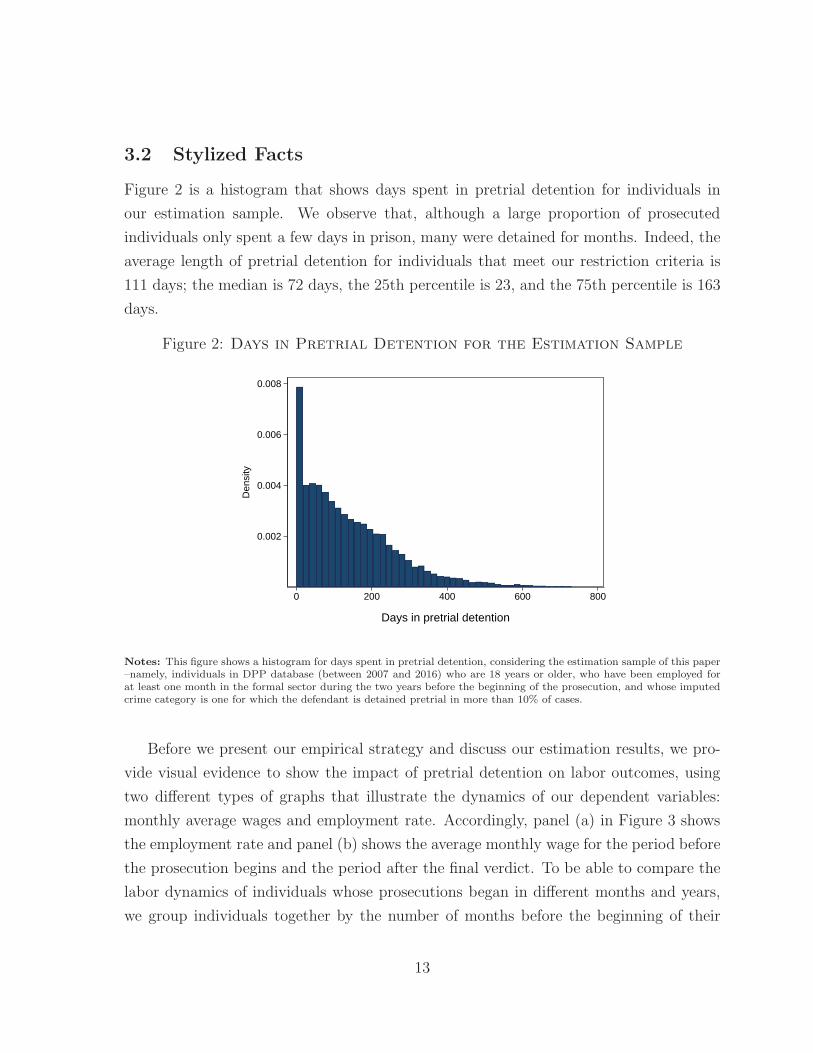
Figure 2 is a histogram that shows days spent in pretrial detention for individuals in

our estimation sample. We observe that, although a large proportion of prosecuted

individuals only spent a few days in prison, many were detained for months. Indeed, the

average length of pretrial detention for individuals that meet our restriction criteria is

111 days; the median is 72 days, the 25th percentile is 23, and the 75th percentile is 163

days.

Figure 2: Days in Pretrial Detention for the Estimation Sample

0.002

0.004

0.006

0.008

Den

sity

0 200 400 600 800

Days in pretrial detention

Notes: This figure shows a histogram for days spent in pretrial detention, considering the estimation sample of this paper–namely, individuals in DPP database (between 2007 and 2016) who are 18 years or older, who have been employed forat least one month in the formal sector during the two years before the beginning of the prosecution, and whose imputedcrime category is one for which the defendant is detained pretrial in more than 10% of cases.

Before we present our empirical strategy and discuss our estimation results, we pro-

vide visual evidence to show the impact of pretrial detention on labor outcomes, using

two different types of graphs that illustrate the dynamics of our dependent variables:

monthly average wages and employment rate. Accordingly, panel (a) in Figure 3 shows

the employment rate and panel (b) shows the average monthly wage for the period before

the prosecution begins and the period after the final verdict. To be able to compare the

labor dynamics of individuals whose prosecutions began in different months and years,

we group individuals together by the number of months before the beginning of their

13

prosecution and by the number of months after their final verdict in order to calculate

the average monthly wage and average employment rate for the individuals in the treat-

ment and control groups. For months before the beginning of the trial the value on the

horizontal axis is negative; for months after the final verdict the value on the horizontal

axis is positive. This implies that the time between −1 and 1 is equal to the duration

of the trial, a variable that is heterogeneous across individuals. The average length of

trial for the treatment group is equal to 254 days with a standard deviation equal to

243. And the average length of trail for the control group is equal to days 167 with a

standard deviation equal to 231.

The second type of graphs present the differences in the employment rate or average

monthly wage between the treatment and the control group. They are presented in

Figure 4.

Figure 3: Employment and Wages Dynamics for the Treatment andControl Groups

(a) Employment rate

0.25

0.30

0.35

0.40

0.45

0.50

Ave

rage

em

ploy

men

t rat

e

−24 −20 −16 −12 −8 −4 0 4 8 12 16 20 24

Months before the beginning of trial and after the final verdict

Treated

Control

(b) Average wages

50,000

100,000

150,000

200,000

Ave

rage

mon

thly

wag

e

−24 −20 −16 −12 −8 −4 0 4 8 12 16 20 24

Months before the beginning of prosecution and after the final verdict

Treated

Control

Notes: These figures show the dynamics for the employment rate (panel (a)) and average wages (panel (b)), pre- andpost-prosecution, for the treatment (triangles) and control groups (circles). Each dot represents the average value ofemployment or monthly wages, for a particular month, X months before the beginning of the prosecution (when X has anegative value on the horizontal axes) or X months after the final verdict (when X has a positive value on the horizontalaxes). Note that X equals zero refers to a period that is a different length for different individuals, lasting from thebeginning of prosecution to the end of trial, including the final verdict.

These plots illuminate a few aspects in the data. First, both before and after treat-

ment, individuals in the control group perform better in the labor market compared to

individuals in the treatment group. During the months before prosecution, control group

14

members have a higher probability of being employed, between 8 pp and 12 pp more on

average. Moreover, their average monthly wages are about 70,000 CLP (or 108 USD)

higher, which represents 37% of the average monthly wage of the control group.12 Sec-

ond, the parallel trends condition appears to be satisfied. This can be directly observed

in Figure 3 and is also evidenced by the consistency of the pretreatment dynamics in

Figure 4. It is formally tested in Section 5.2. Third, there is a clear, discrete change

after an individual has been subject to pretrial detention in the differences between the

treatment and control groups in both employment rates and average monthly wages,

which supports this paper’s main result. As panel (a) in Figure 4 shows, in the case of

employment rates this change is about 4 pp on average. Panel (b) shows that for aver-

age monthly wages the change is around 18, 000 CLP. Finally, Figure 4 shows that the

increase in the differences in labor outcomes between the treatment and control groups

are more severe immediately after the final verdict, and it also shows that the increase

in these differences does not fade over a period of two years after the end of the trial.

12The treatment group is partially comprised of individuals who make less than the minimum wage.There are three main reasons for this: the probability of being employed is low (between 44% and 51%)and the average wage calculation considers unemployment as zero wages; treatment group members arelikely to have low productivity (and low bargaining power); and, finally, many could be employed in theinformal labor market and therefore their wages are not observable.

15

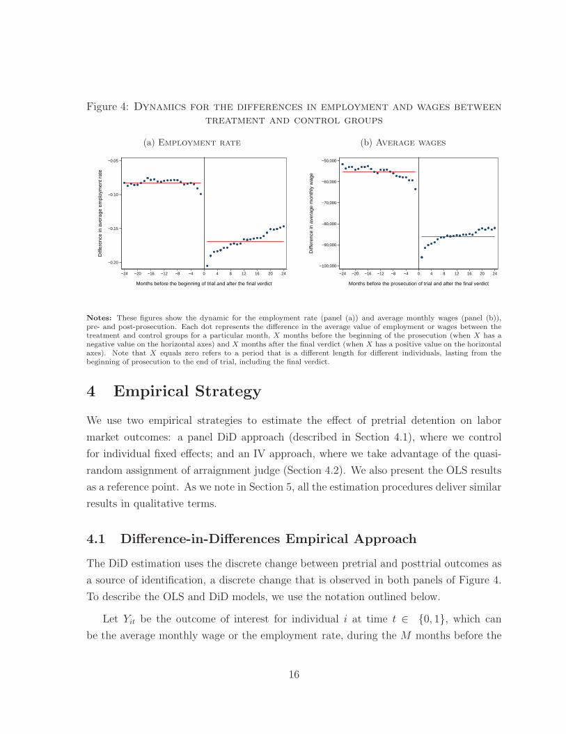
Figure 4: Dynamics for the differences in employment and wages betweentreatment and control groups

(a) Employment rate

−0.20

−0.15

−0.10

−0.05

Diff

eren

ce in

ave

rage

em

ploy

men

t rat

e

−24 −20 −16 −12 −8 −4 0 4 8 12 16 20 24

Months before the beginning of trial and after the final verdict

(b) Average wages

−100,000

−90,000

−80,000

−70,000

−60,000

−50,000

Diff

eren

ce in

ave

rage

mon

thly

wag

e

−24 −20 −16 −12 −8 −4 0 4 8 12 16 20 24

Months before the prosecution of trial and after the final verdict

Notes: These figures show the dynamic for the employment rate (panel (a)) and average monthly wages (panel (b)),pre- and post-prosecution. Each dot represents the difference in the average value of employment or wages between thetreatment and control groups for a particular month, X months before the beginning of the prosecution (when X has anegative value on the horizontal axes) and X months after the final verdict (when X has a positive value on the horizontalaxes). Note that X equals zero refers to a period that is a different length for different individuals, lasting from thebeginning of prosecution to the end of trial, including the final verdict.

4 Empirical Strategy

We use two empirical strategies to estimate the effect of pretrial detention on labor

market outcomes: a panel DiD approach (described in Section 4.1), where we control

for individual fixed effects; and an IV approach, where we take advantage of the quasi-

random assignment of arraignment judge (Section 4.2). We also present the OLS results

as a reference point. As we note in Section 5, all the estimation procedures deliver similar

results in qualitative terms.

4.1 Difference-in-Differences Empirical Approach

The DiD estimation uses the discrete change between pretrial and posttrial outcomes as

a source of identification, a discrete change that is observed in both panels of Figure 4.

To describe the OLS and DiD models, we use the notation outlined below.

Let Yit be the outcome of interest for individual i at time t ∈ {0, 1}, which can

be the average monthly wage or the employment rate, during the M months before the

16

beginning of the trial (when t = 0) and during the M months after the final verdict

(when t = 1). In our empirical implementation M is equal to 6 or 24 months. Treated

individuals (PreTriali = 1) were incarcerated during the criminal proceedings (or for at

least part of them) and the individuals in the control group (PreTriali = 0) were not

incarcerated during the criminal proceedings.

The DiD and OLS models have different sets of covariates X . The OLS set of co-

variates (Xolsi1 ) includes dummies for gender, Chilean citizenship, ethnicity, pretreatment

average monthly wage, pretreatment employment rate (6 or 24 months before prosecu-

tion), location of the court (by region), type of crime, trial duration, and the year and

month of the sentence. The panel DiD set of covariates (Xpit) include the year and month

when the prosecution began (when t = 0), the year and month of the sentence (when

t = 1), and ωi, which is the fixed effect for individual i.

The parameters of interest are denoted by β. For example, βp is the estimated effect

of pretrial detention using the panel DiD approach (Eq. (2)). The specifications of the

estimated models set out below.13

OLS:

Yi,1 = α + βolsPreTriali + γ′Xolsi1 + ǫi1. (1)

Difference-in-differences, panel data:

Yi,t = α1[t = 1] + βpPreTriali ∗ 1[t = 1] + γ′Xpit + ωi + ǫit, t ∈ {0, 1}. (2)

The identification of βp requires that there is no variable that varies between t = 0

and t = 1 and that influences both the probability of being incarcerated during the pros-

ecution and labor market outcomes. This assumption is indirectly tested by presenting

the labor outcome trends for the treated and control groups before treatment (Subsection

4.1.1).14

In Appendix D.1 we also show the results from a cross-sectional DiD and a DiD

matching estimator. The results are very stable across different DiD specifications.

131[A] is an indicator function that takes the value of one when A is true and zero otherwise.

14A good discussion on the importance of a proper understanding of the reasons why individuals fromthe treated and control groups have different pretreatment outcomes can be found in Kahn-Lang andLang (2019).

17

4.1.1 General Difference-in-Differences Approach

Following Duflo (2001), we generalize the panel DiD identification strategy to an inter-

action terms analysis by allowing for period-by-period contrasts. In the literature, this

is commonly referred to as an “event study” approach. This approach is suitable for

presenting the effect of pretrial detention on labor outcomes, a test of parallel trends,

and the potential fading out of the estimated effect, all in the same figure.

By using the month as the time unit, where the omitted category is the month that

occurred 24 months before the beginning of prosecution, we run the following model:

Yit =24∑

n=−23∧n 6=0

βnPreTriali ∗ 1[t = n] +24∑

n=−23∧n 6=0

δn ∗ 1[t = n] + ωi + ǫit, (3)

where i is the individual subindex, t is the period subindex, and ωi is the fixed effect

for individual i. Given this model, we are interested in the point estimates of βn (and

their confidence intervals), where each coefficient βn can be interpreted as an estimate

of the impact of the pretrial detention on period n relative to the first period (n = −24,

24 months before treatment), which is the omitted category.15 Because the first 24

periods (including period -24, the reference category) are pretreatment, the identification

strategy is suitable for causal interpretation to the extent that the point estimates of βn,

where n < 0, are close to zero. Conditional on the point estimates of βn being close to

zero, which is a simple way to test parallel trends, the point estimates for βn, where n > 0,

can be interpreted as the effects of pretrial detention after n month post treatment.

4.2 Instrumental Variable

The instrumental variable considered in this paper is a leave-out mean that captures how

the (quasi-random) assignment of the arraignment judge impacts the probability of an

individual being subject to pretrial detention.

To construct this instrumental variable we use a dataset that includes all criminal

records, with and without data on labor outcomes. More specifically, this is the sample

described in the first column of Table 1. From this starting point, we only consider courts

15Note that in the estimation we do not consider n = 0.

18

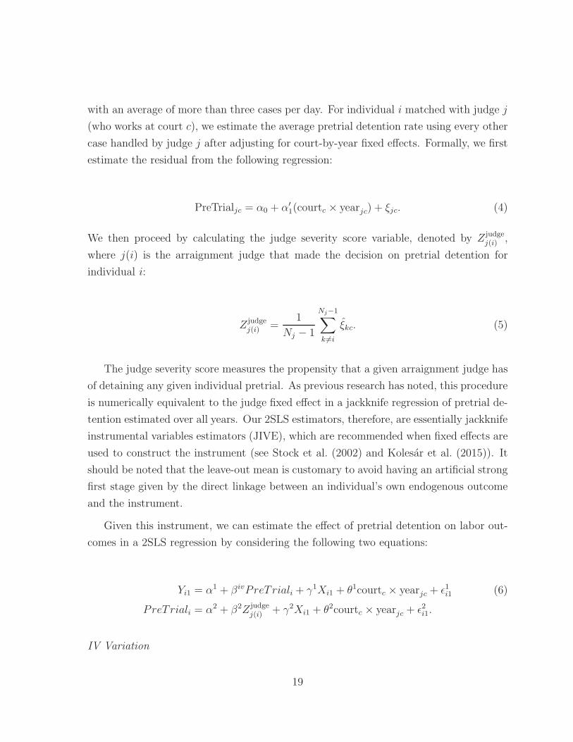
with an average of more than three cases per day. For individual i matched with judge j

(who works at court c), we estimate the average pretrial detention rate using every other

case handled by judge j after adjusting for court-by-year fixed effects. Formally, we first

estimate the residual from the following regression:

PreTrialjc = α0 + α′1(courtc × yearjc) + ξjc. (4)

We then proceed by calculating the judge severity score variable, denoted by Z judgej(i) ,

where j(i) is the arraignment judge that made the decision on pretrial detention for

individual i:

Z judgej(i) =

1

Nj − 1

Nj−1∑

k 6=i

ξkc. (5)

The judge severity score measures the propensity that a given arraignment judge has

of detaining any given individual pretrial. As previous research has noted, this procedure

is numerically equivalent to the judge fixed effect in a jackknife regression of pretrial de-

tention estimated over all years. Our 2SLS estimators, therefore, are essentially jackknife

instrumental variables estimators (JIVE), which are recommended when fixed effects are

used to construct the instrument (see Stock et al. (2002) and Kolesar et al. (2015)). It

should be noted that the leave-out mean is customary to avoid having an artificial strong

first stage given by the direct linkage between an individual’s own endogenous outcome

and the instrument.

Given this instrument, we can estimate the effect of pretrial detention on labor out-

comes in a 2SLS regression by considering the following two equations:

Yi1 = α1 + βivPreTriali + γ1Xi1 + θ1courtc × yearjc + ǫ1i1 (6)

PreTriali = α2 + β2Z judgej(i) + γ2Xi1 + θ2courtc × yearjc + ǫ2i1.

IV Variation

19

In Figure 5 we present the distribution of the instrumental variable. The sample used to

construct the instruments consists of 907 judges. The average judge handles 367 cases

per year. In the estimation sample, the mean of the severity score variable is −0.00001

with a standard deviation of 0.0414. The severity measure ranges from −0.060 (5th

percentile) to 0.065 (95th percentile), which implies that moving from a less severe to a

more severe judge is associated with a 5 pp increase in being detained pretrial.

Figure 5: Distribution of the Judge Severity Instrument and theNon-parametric First Stage

0.11

0.13

0.15

0.17

0.19 Residualized R

ate of Pretrial D

etention

0

.02

.04

.06

.08

Fra

ctio

n of

Sam

ple

−0.05 −0.03 0.00 0.03 0.05Judge Severity

Note: This figure reports the distribution of the judge severity measure that is estimated following the procedure describedabove. It also shows the non-parametric estimation of the relationship between the judge severity score and the residualizedrate of pretrial detention.

4.2.1 IV validity

In order to interpret the 2SLS estimates as a local average treatment effect, the following

four conditions must be met (Imbens and Angrist (1994)): (i) a non-trivial first stage, (ii)

independence of the instrument, (iii) exclusion of the instrument, and (iv) monotonicity.

In what follows, we will discuss each of these conditions.

A Non-trivial First Stage

20

Figure 5 shows the effect of the judge severity score on whether or not an individual is

detained pretrial, estimated via a local linear regression of the former against the latter

after controlling for court-by-year fixed effects (i.e., the residualized rate). The pretrial

detention status varies monotonically along the judge severity score in a fairly linear

fashion.

The first stage estimation is presented in Table 3. It shows that our instrumental

variable is a good predictor of whether an individual is detained pretrial. We present two

specifications: (1) controlling for employment outcomes during the 6 months before the

prosecution and (2) controlling for employment outcomes during the 24 months before

the prosecution. Both specifications deliver similar results. The magnitudes suggest that

if an accused individual is assigned to a judge who is 10 pp more likely to give pretrial

detention, then that individual is between 3.7 pp and 4.2 pp more likely to be detained

pretrial.

21

Table 3: First stage: judge severity score

(1) (2)

Judge severity IV 0.373*** 0.417***(0.036) (0.037)

Six months of wages -0.000***(0.000)

Six months of employment -0.034***(0.004)

Two years of wages -0.000***(0.000)

Two years of employment -0.049***(0.005)

Male 0.046*** 0.045***(0.004) (0.004)

non-Chilean citizen 0.043* 0.028(0.022) (0.023)

Indigenous 0.010 0.015(0.017) (0.018)

Days in judicial process 0.000*** 0.000***(0.000) (0.000)

Crime severity 0.009*** 0.009***(0.000) (0.000)

Fixed term contract 0.013*** 0.005(0.003) (0.003)

Sector = Mining -0.006 -0.006(0.014) (0.014)

Sector = Manufacturing -0.015** -0.016**(0.006) (0.006)

Sector = Electricity-Gas-Water -0.042 -0.040(0.028) (0.031)

Sector = Construction 0.013** 0.016***(0.005) (0.006)

Sector = Commerce -0.017*** -0.017***(0.006) (0.006)

Sector = Services -0.004 -0.005(0.005) (0.005)

Sector = Transportation-Communication -0.008 -0.007(0.007) (0.007)

Firm size = Small 0.006 0.007(0.004) (0.005)

Firm size = Medium 0.000 0.001(0.005) (0.005)

Firm size = Big -0.004 -0.001(0.004) (0.004)

Constant -0.130*** -0.113***(0.009) (0.009)

F test 106.84 128.19Observations 68,814 61,479Court-by-time fixed effects Yes Yes

Notes: This table reports first-stage results for the linear IV model that estimates theeffect of pretrial detention on labor outcomes. The IV is the judge severity measure,which is estimated following the procedure described in Subsection 4.2. In Column (1)we control for employment outcomes during the 6 months before the prosecution begins,and in Column (2) we control for employment outcomes during the 24 months beforethe prosecution begins. The model is estimated on the sample described in the notes forTable 2. Regression includes year interacted with court fixed effects. Robust standarderrors are clustered at the judge level in parentheses. Statistical significance at 1%, 5%,and 10% is indicated by ***, **, and *, respectively.

22

Independence

The independence of the instrument is a key condition to validate the IV approach. In

order for this condition to be met, the instrument must be as good as random assign-

ment. To verify that this assumption holds in our context, Table 4 presents the same

kind of analysis that would be performed in an actual experiment to assess the quality

of its randomization. The first column displays the coefficients of a regression of the en-

dogenous variable (i.e., pretrial detention) against the covariates described in the rows.

The second column shows the same regression but with the instrumental variable (i.e.,

judge severity) as the dependent variable. In both models we control for year interacted

with court fixed effects (the level at which judges are quasi-randomly assigned). That

said, the null hypothesis of all parameters equal to zero, tested using the F-test, does

not consider these court-by-year covariates. In Table 4 we note that gender, pretreat-

ment labor outcomes, crime severity, and employer sector dummies are highly predictive

of being subject to pretrial detention, whereas almost none of these variables seem to

predict the severity of the assigned judge. This is corroborated further by the p-value

given by the joint significance test, which is not able to reject the null hypothesis that

all the coefficients are equal to zero (p-value = 0.35).

It is the combination of the two regressions presented in Table 4 that makes this test

a convincing approach. In this table, the first column shows that these covariates are

very relevant for predicting the endogenous variable, and the second column shows that

the relevant covariates are not correlated with the instrumental variable, in a similar

fashion to how one would test the validity of a randomized controlled trial.

23

Table 4: Randomization test for judge severity score

Pretrial Detention Judge severity IV

Male 0.045*** -0.000(0.004) (0.001)

non-Chilean citizen 0.027 -0.004**(0.023) (0.002)

Indigenous 0.015 0.000(0.018) (0.001)

Days in judicial process 0.000*** -0.000(0.000) (0.000)

Two years of wages -0.000*** -0.000(0.000) (0.000)

Two years of employment -0.049*** 0.000(0.005) (0.001)

Crime severity 0.009*** 0.000(0.000) (0.000)

Fixed term contract 0.005 0.000(0.003) (0.000)

Sector = Mining -0.006 -0.001(0.014) (0.002)

Sector = Manufacturing -0.016*** -0.000(0.006) (0.001)

Sector = Electricity-Gas-Water -0.039 0.002(0.031) (0.004)

Sector = Construction 0.016*** 0.000(0.006) (0.001)

Sector = Commerce -0.017*** 0.000(0.006) (0.001)

Sector = Services -0.005 -0.000(0.005) (0.001)

Sector = Transportation-Communication -0.007 -0.000(0.007) (0.001)

Firm size = Small 0.007 -0.000(0.005) (0.000)

Firm size = Medium 0.001 -0.001*(0.005) (0.001)

Firm size = Big -0.001 -0.001*(0.004) (0.000)

Constant -0.113*** 0.000(0.009) (0.002)

Joint Test 0.0000 0.3533Observations 61,479 61,479Court-by-time fixed effects Yes Yes

Notes: This table reports the reduced form results that test the random assignment of cases to arraignment judges. Thejudge severity measure is estimated following the procedure described in Subsection 4.2. Column 1 presents estimatesfrom an OLS regression of pretrial detention on the variables listed and year interacted with court fixed effects. Column2 reports estimates from an OLS regression of the judge severity IV on the variables listed and year interacted with courtfixed effects. The p-value reported at the bottom of columns 1 and 2 (named Joint Test) is for an F-test of the jointsignificance of the variables listed in the rows with the standard errors clustered at the judge level. Therefore, the F-testdoes not include the year interacted with court fixed effects in the null hypothesis. Robust standard errors clustered atthe judge level are in parentheses. Statistical significance at 1%, 5%, and 10% is indicated by ***, **, and *, respectively.

24

Exclusion

The quasi-random assignment of cases to judges is sufficient for a causal interpretation

of the reduced form impact of being assigned to a more severe arraignment judge (see

reduced form estimates in Appendix A). The interpretation of the IV estimates as the

impact of pretrial detention on labor outcomes, however, also requires that the arraign-

ment judge assignment only impacts individuals’ outcomes through the probability of

being subject to pretrial detention and not through any other channel. Conditional on

deciding to begin a criminal proceeding, this is likely to be the case in our setting be-

cause the only role of these judges is to prescribe precautionary measures. Recall that

the verdict is determined by three different judges in an oral proceedings court.16

That said, we follow Bald et al. (2019) by presenting suggestive evidence that the ex-

clusion restriction is met in our setting. In Table 5, we show the results of our test to

see whether judge severity is correlated with other trial outcomes for the subgroup of

accused individuals who were detained pretrial. More specifically, we test the correlation

between our measure of judge severity and the duration of the pretrial detention, which

ends when the final trial verdict is given (whether a custodial sentence is passed or not).

As Table 5 shows, we find no evidence of a correlation between these variables, which is

consistent with the exclusion assumption.

16A arraignment judge may also give a sentence in a case if it is simple enough and takes place inan abbreviated trial process for non-severe crimes only. In general, it is defined during the arraignmenthearing at the guarantee court. Given that our focus is on more severe crimes, we do not consider thesescases.

25

Table 5: Exclusion restriction test: the impact of judge severity onsentencing outcomes

Days in pretrial detention Custodial sanction

Judge severity IV 30.44 -0.15(26.47) (0.13)

Two years of wages -0.00 -0.00(0.00) (0.00)

Two years of employment -11.38 0.00(7.12) (0.03)

Male 7.99 -0.05**(5.00) (0.02)

non-Chilean citizen 11.97 0.06(12.04) (0.08)

Indigenous 11.29 0.07(12.14) (0.05)

Days in judicial process 0.48*** 0.00***(0.03) (0.00)

Crime severity 0.98*** -0.00(0.11) (0.00)

Fixed term contract -0.55 -0.01(2.98) (0.02)

Sector = Mining 22.19* 0.11(12.61) (0.07)

Sector = Manufacturing 0.26 0.00(5.99) (0.03)

Sector = Electricity-Gas-Water -16.17 0.04(18.04) (0.17)

Sector = Construction -2.28 0.01(5.20) (0.02)

Sector = Commerce -1.18 0.03(5.63) (0.03)

Sector = Services -0.29 0.03(5.00) (0.02)

Sector = Transportation-Communication 0.51 0.05*(7.20) (0.03)

Firm size = Small -3.74 -0.01(4.33) (0.02)

Firm size = Medium -0.67 -0.00(4.33) (0.02)

Firm size = Big -3.19 -0.00(3.93) (0.02)

Constant 16.66* 0.62***(9.58) (0.04)

Observations 8,854 8,854Court-by-time fixed effects Yes Yes

Notes: This table presents the correlation, for those who were detained pretrial, between judgeseverity and the duration of the pretrial detention, which ends when the final trial verdict is given(whether a custodial sentence is passed or not), controlling for a set of relevant covariates (includingcourt-by-time fixed effects). Robust standard errors are clustered at the judge level in parentheses.Statistical significance at 1%, 5%, and 10% is indicated by ***, **, and *, respectively.

26

Monotonicity

The monotonicity assumption requires that an accused individual who is detained pretrial

by a lenient judge could have also been detained pretrial by a more severe judge and

viceversa. In the literature, as discussed by both Dobbie et al. (2018) and Bhuller et al.

(2020), a common approach to (indirectly) test this assumption is to estimate the first-

stage regression for different subgroups and obtain point estimates for the instrument

that are all of the same sign and have similar magnitudes. The result of this approach for

our study is illustrated in panel A of Table 6, where we present the first-stage estimations

for different subgroups of imputed crimes, by individuals’ pretreatment average monthly

wages (below and above the median), the size of the individual’s pretreatment employer

(big companies versus the rest), and crime severity (below and above the median). The

table shows that in all cases but one (below median crime severity), the point estimates

for the first stage are very similar across different groups. Even in the one case where

the point estimate is different, We do not observe a flip in the sign of the estimated

coefficient. These results suggest that the monotonicity assumption holds in our setting.

27

Tab

le6:

Monotonicitytest

:First

-stageest

imationsfordifferentgroups

PanelA:First-StageIm

pactofJudgeseverity,bySubgroup

abov

emed

ian

wages

below

med

ian

wages

big

andmed

ium

companies

smallandmicro

companies

abov

emed

ian

crim

eseverity

below

med

ian

crim

eseverity

JudgeseverityIV

0.330***

0.439***

0.386***

0.400***

0.453***

0.263***

(0.046)

(0.055)

(0.046)

(0.061)

(0.058)

(0.041)

Observations

35,426

33,514

45,236

23,704

36,970

31,970

PanelB:First-StageIm

pactofJudgeseverity,byReverseSample

Calculation

forSubgroups

abov

emed

ian

wages

below

med

ian

wages

big

andmed

ium

companies

smallandmicro

companies

abov

emed

ian

crim

eseverity

below

med

ian

crim

eseverity

JudgeseverityIV

0.160***

0.301***

0.154***

0.229***

0.081

0.029

(0.032)

(0.054)

(0.032)

(0.050)

(0.053)

(0.027)

Observations

35,352

33,456

45,057

23,680

36,825

31,892

Notes:In

panel

A,this

table

reportsfirst-stageresu

ltsforthelinearIV

model

thatestimatestheeff

ectofpretrialdeten

tiononlaboroutcomes

bycrim

eseverity.

Panel

Bsh

owstheestimationsofthefirst-stagemodels,

wheretheleav

e-outinstru

men

tis

recalculated

fordifferen

tsu

bgroupsusingall

casesoutsideofthese

subgroups.

Theregressionsin

both

panelsare

estimated

usingthesample

asdescribed

inthenotesofTable

2.

Theregressionsincludeyearinteracted

with

court

fixed

effects.Robust

standard

errors

clustered

atthejudgelevel

inparentheses.Statisticalsignificance

at1%,5%,and10%

isindicatedby***,**,and*,

resp

ectively.

28

To provide more indicative evidence to support the monotonicity assumption, we

follow Bald et al. (2019) by estimating the first-stage models and recalculating the leave-

out instrument for different subgroups using all cases outside of these subgroups. We

present this analysis in panel B of Table 6. We observe that the point estimates are

consistently positive and always statistically different from zero. The results from this

approach also suggest that the monotonicity assumption holds in our setting. In Table

13 (Appendix B) we replicate these two tests but grouping the data by type of crime.

As in the case of Table 6, both tests present evidence supporting monotonicity.

5 Results

In this section we present the results of the panel DiD and IV approaches. We also

provide the OLS estimates as a point of reference.

5.1 Main results

For the short-term impact of pretrial detention on employment, the dependent variable

is calculated in t = 0 as the employment rate during the six months before treatment

and in t = 1 as the employment rate during the six months after treatment. Regarding

the timing of these effects, note that before treatment refers to the period before the

beginning of prosecution and after treatment refers to the period after the verdict. Table

7 shows that the short-term impact of pretrial detention on the employment rate is −9.8

pp in the case of the DiD estimation (column 2) and −17.8 pp in the case of the IV

specification (column 3). These effects represent a decrease in the likelihood of being

employed of between 21.1% (9.8/46.5) and 39.5% (17.8/45). Regarding the mid-term

effect, in which case the dependent variable is calculated in t = 0 as the employment

rate during the 24 months before treatment and in t = 1 as the employment rate during

the 24 months after treatment, the impact of pretrial detention on the employment rate is

−8.5 pp and −21.0 pp for the DiD estimation and the IV estimation, respectively. These

point estimates represent a decrease in the likelihood of being employed of between 18.4%

(8.5/46.3) and 46.2% (21.0/45.5). All these point estimates are statistically significant

at the 1% level.

For the impact of pretrial detention on the average monthly wage, Table 8 reports

29

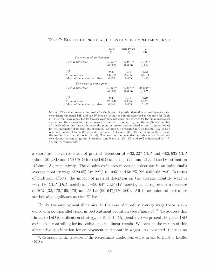
Table 7: Effect of pretrial detention on employment rate

OLS DiD Panel IV(1) (2) (3)

Six months of employment

Petrial Detention -0.120∗∗∗ -0.098∗∗∗ -0.178∗∗

(0.003) (0.003) (0.084)

R2 0.30 0.76 0.32Observations 142,419 285,358 68,814Mean of dependent variable 0.437 0.465 0.450

Two years of employment

Petrial Detention -0.112∗∗∗ -0.085∗∗∗ -0.210∗∗∗

(0.003) (0.003) (0.075)

R2 0.29 0.75 0.29Observations 126,547 253,550 61,479Mean of dependent variable 0.441 0.463 0.455

Notes: This table presents the results for the impact of pretrial detention on employment rate,considering the panel DiD and the IV models (using the sample described in the note for Table2). The results are presented for two separate time horizons: the average for the six months afterverdict and the average for the two years after verdict. In order to group the results of a numberof specifications into one table, only the point estimates and standard errors (in parentheses)for the parameter of interest are presented. Column (1) presents the OLS results (Eq. 1) as areference point. Column (2) presents the panel DiD model (Eq. 2) and Column (3) presentsthe results from the IV model (Eq. 6). The mean of the dependent variable is calculated onlyconsidering the control group. Statistical significance at 1%, 5%, and 10% is indicated by ***,**, and *, respectively.

a short-term negative effect of pretrial detention of −32, 227 CLP and −92, 635 CLP

(about 50 USD and 150 USD) for the DiD estimation (Column 2) and the IV estimation

(Column 3), respectively. These point estimates represent a decrease in an individual’s

average monthly wage of 20.0% (32, 227/161, 095) and 56.7% (92, 635/163, 293). In terms

of mid-term effects, the impact of pretrial detention on the average monthly wage is

−32, 176 CLP (DiD model) and −90, 647 CLP (IV model), which represents a decrease

of 20% (32, 176/160, 170) and 53.1% (90, 647/170, 560). All these point estimates are

statistically significant at the 1% level.

Unlike the employment dynamics, in the case of monthly average wage there is evi-

dence of a non-parallel trend in pretreatment evolution (see Figure 7).17 To address this

threat to DiD identification strategy, in Table 14 (Appendix C) we present the panel DiD

estimation controlling for individual specific linear trends. We present the results of this

alternative specification for employment and monthly wages. As expected, there is no

17A discussion on the relevance of the pretreatment employment evolution can be found in Loeffler(2018).

30

relevant difference when comparing the point estimates of the employment models with

and without these individuals’ trends as a covariates. On the contrary, there is a clear

difference when comparing the point estimates of the monthly wage models with and

without these individuals’ trends as a covariate. In particular, we see that this violation

of parallel trend could explain 25% of the point estimate that we find in column 2 (Table

8). That said, this issue does not affect the identification strategy for the IV estimation.

Two more aspects illustrated by these tables are worth highlighting. First, the magni-

tudes are very similar if we compare short-term to mid-term effects. The mid-term effect

estimation, however, requires more months of data posttreatment. We therefore have a

smaller sample and the magnitudes for mid-term effects must be taken with a note of

caution. Indeed, as shown in Section 5.2, when we use the same sample – and specifica-

tion – to estimate the effect of pretrial detention for different periods after treatment, we

find a clear reduction in the effect on employment over time in the point estimates. This

is less clear in the case of wages. Second, in the cases of both employment and wages,

OLS estimations present larger point estimates relative to DiD estimations . This dif-

ference in magnitude is consistent with the fact that, unlike the DiD models, the OLS

estimation does not control for unobserved variables that are stable through time and

affect labor market outcomes. The comparison between the OLS estimation and the IV

estimation is less clear because the IV estimation is based on a different sample (as a

result of the restrictions required to use the judge severity instrument) and identifies the

causal effect for the compliers (i.e., the LATE).

31

Table 8: Effect of pretrial detention on average wage

OLS DiD Panel IV(1) (2) (3)

Six months of wages

Petrial Detention -42,380∗∗∗ -32,227∗∗∗ -92,635∗∗

(1,178) (1,337) (38,019)

R2 0.56 0.87 0.58Observations 142,419 285,358 68,814Mean of dependent variable 158,304 161,095 163,293

Two years of wages

Petrial Detention -41,315∗∗∗ -32,176∗∗∗ -90,647∗∗

(1,230) (1,385) (46,093)

R2 0.51 0.85 0.52Observations 126,547 253,550 61,479Mean of dependent variable 164,986 160,170 170,560

Notes: This table presents the results for the impact of pretrial detention on monthly wages,considering the panel DiD and the IV models (using the sample described in Table 2). The resultsare presented for two time horizons: the average for the six months after verdict, and the averagefor the two years after verdict. In order to group the results of a number of specifications in onetable, only the point estimates and standard errors (in parentheses) for the parameter of interestare presented. Column (1) presents the OLS results (Eq. 1), which is a useful reference point.Column (2) presents the panel DiD model (Eq. 2) and Column (3) presents the results from theIV model (Eq. 6). The mean of the dependent variable is calculated only considering the controlgroup. Statistical significance at 1%, 5%, and 10% is indicated by ***, **, and *, respectively.

5.2 General Approach (event study)

Figures 6 and 7 present the estimations of equation (3) – that is, the panel DiD model

that allows us to estimate an effect for each period for the impact of pretrial detention

on employment rates and average monthly wages. The dynamics of these two plots can

be summarized in three findings.

First, for employment rates the empirical strategy does not find a statistically sig-

nificant effect before treatment,18 which is consistent with the parallel trend condition.

Because pretrial detention occurs at different times for different individuals, it is unlikely

that another treatment (i.e., policy) occurs at the same time as pretrial detention for all

individuals. And as the relevant test to ensure the identification of the causal parameter

in the DiD model is the verification of the pretreatment parallel trends assumption, Fig-

ure 6 supports the idea that the DiD estimates can be interpreted as a causal effect. For

average monthly wages, there is clear evidence that the parallel trend condition is not

18There is a point estimate that is statistically significant but quantitatively irrelevant in the lastperiod before treatment

32

met (Figure 7). For this reason, we also estimate that model including a linear trend for

treated as a covariate. Second, there is a statistically significant effect posttreatment,

the magnitudes of which are in line with the point estimates presented in Tables 7 and

8 at the beginning of this section. Third, and finally, there is a clear reduction in the

point estimates in the case of employment over time, but the trend is less clear for wages.

That said, for both measures, the effect is still present in the average outcome measured

18 to 24 months after treatment.

Figure 6: Impact of Pretrial Detention on Employment Rate (GeneralApproach)

−0.15

−0.10

−0.05

0.00

0.05

Effe

ct o

n em

ploy

men

t

−24 −20 −16 −12 −8 −4 0 4 8 12 16 20 24

CI at 95% Point estimate

Notes: This figure shows the point estimates and their 95% confidence intervals for the effect of pretrial detention onemployment rate by estimating Equation 3, considering the estimation sample described in Table 2.

33

Figure 7: Impact of Pretrial Detention on Average Monthly Wage(General Approach)

−50,000

−40,000

−30,000

−20,000

−10,000

0E

ffect

on

wag

e

−24 −20 −16 −12 −8 −4 0 4 8 12 16 20 24

CI at 95% Point estimate

Notes: This figure shows the point estimates and their 95% confidence intervals for the effect of pretrial detention onaverage monthly wage by estimating Equation 3, considering the estimation sample described in Table 2.

5.3 Robustness Analysis

In Appendix D we present a set of results to study the robustness of our main conclusions

to alternative specifications. We begin our robustness checks by estimating alternative

DiD models – namely, a cross-sectional DiD model and a matching DiD model(Heckman

et al. (1997)). Tables 15 and 16 (in Appendix D.1) show that our point estimates are

very stable across the alternative specifications for DiD models.

Our second robustness analysis is to estimate our models with a different estimation

sample. Here, we consider crimes for which more than 5% of cases receive pretrial

detention rather than the 10% threshold used in our main specification. As shown in

Tables 17 and 18 (in Appendix D.2), the sample size is increased because of the way it

is constructed, but the point estimates are very similar to the values presented in Tables

7 and 8.

Our final robustness analysis is to estimate the DiD model considering the estimation

sample used for the IV estimation. Here, given that the instrument construction requires

that only courts with more than three cases per day on average are considered, we

34

cannot use the full estimation sample. This exercise is presented in Tables 19 and 20 (in

Appendix D.3). The tables clearly show the difference s between the IV and the DiD

point estimates are not due to sample differences. Thus, they should be because of the

heterogeneous impact of the treatment and the local nature of the causal effect that is

shown by the IV estimation.

5.3.1 Heterogeneity

In this subsection we explore two dimensions for the heterogeneous impact of pretrial

detention on labor outcomes: how the impact of pretrial detention depends on its length,

and the effect of pretrial detention by restricting the sample to those individuals who

did not receive a custodial sentence as a result of the verdict of their trial. In our main

specification, we do not restrict the sample based on trial verdict.

The impact by time imprisoned

Using a panel DiD model, similar to the one used to estimate the average effect, we can

study whether the effect of pretrial detention on labor outcomes increases with the length

of the pretrial detention. To study this heterogeneity, we extend the model presented

in Equation (2), defining terciles (Ti ∈ {1, 2, 3}) for the distribution of days detained

pretrial. Note that the amount of time spent in pretrial detention varies vastly over

terciles. The first tercile are imprisoned for 35 days on average, whereas it rises to 122

for the second tercile and 296 for the third. Then, the estimated model is as follows:

Yi,t = α1[t = 1]+βp1PreTriali∗1[Ti = 1]∗1[t = 1]+βp

2PreTriali∗1[Ti = 2]∗1[t = 1]+

βp3PreTriali ∗ 1[Ti = 3] ∗ 1[t = 1] + γ′Xp

it + ωi + ǫit, t ∈ {0, 1}. (7)

The estimated parameters (βp1 , β

p2 , and βp

3) are presented in Figures 8 and 9. The

figures show the average treatment effect for the treated individuals by tercile. As a

reference point, we also include the average treatment effect for the entire estimated

sample (shown by the red line), and the point estimates presented in Tables 7 and 8. In

all cases, for both the employment rate and average monthly wage, for both short and

mid term, there is a clear step gradient pattern for the magnitudes of the treatment effect

35

as individuals spend more time in pretrial detention. That said, for the three terciles

defined for this approach the effect is statistically significant.

Specifically, the short-term effects on employment rate for the first, second, and third

terciles are −4.5 pp, −8.5 pp, and −16.5 pp, respectively. Regarding the mid-term

effects, the numbers are −3.5 pp, −7.0 pp, and −15.1 pp. Thus, the mid-term effect for

the third tercile represents a decrease of 33% (15.1/46.3). For average monthly wages,

the corresponding short-term effects are −17, 686 CLP, −26, 810 CLP, and −52, 900 CLP.

These numbers are equal to −17, 650, −25, 213, and −54, 511 in the mid term. The effect

on the third tercile represents a decrease of 34% (54, 511/160, 170).

Figure 8: Effect of Pretrial Detention on Employment Rate by theDuration of Pretrial Detention

(a) short-term effect: 6 months

−0.20

−0.15

−0.10

−0.05

0.00

Impa

ct o

n em

ploy

men

t

Tercile 1: 35 days in average Tercile 2: 122 days in average Tercile 3: 296 days in average

CI at 95% Point estimate

(b) mid-term effect: 24 months

−0.15

−0.10

−0.05

0.00

Impa

ct o

n em

ploy

men

t

Tercile 1: 35 days in average Tercile 2: 122 days in average Tercile 3: 296 days in average

CI at 95% Point estimate

Notes: These figures show the point estimates and their 95% confidence intervals for the effect of pretrial detention onemployment rate by estimating model for the three terciles of pretrial detention duration (Equation 7), considering theestimation sample described in Table 2.

The impact for individuals released after the final trial verdict

Given that pretrial detention may affect the probability of post-verdict incarceration

(discussed in the Section 6), it is more challenging to estimate the causal effect of pretrial

detention on labor outcomes for individuals not incarcerated as a result of their final trial

verdict. That said, in Appendix E.1 we show that this potential source of bias can be

overcome by the panel DiD approach under reasonable assumptions, which is not the

36

Figure 9: Effect of Pretrial Detention on Average Monthly Wage bythe Duration of Pretrial Detention

(a) short-term effect: 6 months

−60,000

−50,000

−40,000

−30,000

−20,000

−10,000

Impa

ct o

n w

age

Tercile 1: 35 days in average Tercile 2: 122 days in average Tercile 3: 296 days in average

CI at 95% Point estimate

(b) mid-term effect: 24 months

−60,000

−50,000

−40,000

−30,000

−20,000

−10,000

Impa

ct o

n w

age

Tercile 1: 35 days in average Tercile 2: 122 days in average Tercile 3: 296 days in average

CI at 95% Point estimate

Notes: These figures show the point estimates and their 95% confidence intervals for the effect of pretrial detention onaverage monthly wage by estimating model for the three terciles of pretrial detention duration (Equation 7), consideringthe estimation sample described in Table 2.

case for the IV estimation. Thus, to estimate the effect for this specific group, we only

consider the panel DiD estimation.

Tables 21 and 22 in Appendix E present the results of this DiD estimation. As the

tables show, the magnitude of the point estimates is between one-third and one-half

lower when we restrict the sample to those individuals who were released from pretrial

detention after the final verdict. These differences can be explained by the heterogeneity

in the treatment effect (given that they use different samples) or by the fact that the

treatment is different between the two empirical settings. In the main specification we

allow for an impact of pretrial detention through its effect on increasing the probability

of a post-verdict custodial sentence. This point will be discussed in the next section.

6 Mechanisms

There are several different mechanisms that may explain our results, we focus on three.

Firstly, it could be that the impact of pretrial detention on labor outcomes is the general

and natural effect of spending time outside of the labor market during the trial, and its

lasting effect on future (post-verdict) labor market performance. We call this explanation

37

the labor market hypothesis ; the effect here is explained, for example, because individuals

are fired during pretrial detention and post-verdict they have problems in finding a new

job, as it were the case for any poor individual who loses his job. In this case, the pretrial

detention only impacts future labor outcome through its impact on contemporaneous

(during trial) employment participation. Secondly, it could be that pretrial detention

carries an extra and specific impact on labor outcomes due to incarceration itself. For

example, in the hiring process previously incarcerated people are discriminated. We call

this explanation the social stigma hypothesis : the reason for the individuals absence from

the labor market is relevant, not just their non-participation. Finally, it could be that the

effect of pretrial detention on post-verdict labor market outcomes is due to its positive

effect on the probability of post-verdict incarceration, and we call this explanation the

labor incapacitation hypothesis.

6.1 The relevance of the labor market hypothesis

We assess the quantitative relevance of the labor market hypothesis in different ways.

First, we compare the effect of pretrial detention to the effect of losing a job due to

a negative shock beyond the individual’s control. Specifically, we compare our pretrial

detention impacts to the effect of losing a job due to a firm bankruptcy. To estimate

the effect of a firm bankruptcy on wages and employment we use both the treatment

and control group samples are used, but we only consider labor outcome data before

prosecution (i.e. before our treatment). We divide the period before the beginning

of prosecution into three subperiods: between 17 and 24 months before prosecution

(treating this as the period before the firm bankruptcy), between 9 and 16 months before

prosecution (treating this as the period during which the firm would go bankrupt), and

between 1 and 8 months before prosecution (treating this as the period after the potential

bankruptcy, i.e., after the individual’s job loss). In this context, treated individuals are

those who were working at firm j for 17 months before prosecution, and firm j went

bankrupt between 9 and 16 months before the prosecution. Naturally, the control group

is composed of individuals who were working at firm j for 17 months before prosecution,

but firm j did not go bankrupt between 9 and 16 months before the prosecution. As in our

panel DiD specification, we use data on wages and employment pre- and posttreatment

–namely, labor outcome averages between 17 and 24 months before prosecution and

38

between 1 and 8 months before prosecution. In order to generate a fair comparison, we

replicate our panel DiD estimation on the effect of pretrial detention on labor outcomes,

considering the six months before and after the prosecution, but we restrict the sample

to those individuals who were working one month before the beginning of prosecution,

as we did in the firm bankruptcy estimation.

Tables 9 and 10 present the results of this exercise for employment rate and aver-

age monthly wages. In the case of the employment rate, Table 9 shows that the firm

bankruptcy impact is about one-half of the pretrial detention effects. Table 10 shows

that the magnitude of the pretrial detention effect is much more relevant than the mag-

nitudes of the impact of firm bankruptcy, which is not statistically significant. It should

be noted that these point estimates are different from the estimates reported in Tables

7 and 8 because we are attempting to compare the effects of these two treatments and

we therefore restrict the sample to those individuals who were working the month before

the beginning of prosecution.

Our second approach to assessing the quantitative relevance of the labor market

mechanism hypothesis is to take advantage of the fact that we have a firm ID. We can

therefore compare the monthly probability of remaining employed at the same firm pre-

and posttreatment between control and treatment groups. We present these probabilities

in Figure 10, where the triangles represent the probabilities for the treated group and

the circles represent the probabilities for the control. Note that almost all of the points

in figure 10 show the probability of remaining employed at the firm where the individual

was working during the previous month. The first triangle and circle after verdict,

however, cannot refer to the firm where the individual was employed the previous month

because they were being detained pretrial. In fact, they represent the probability of

an individual keeping the job they held immediately before prosecution. As this figure

shows, the dynamics of these probabilities are very similar pre-prosecution and posttrial,

with the exception of the first value after the trial. This means that, conditional on

having a job the month after the verdict (i.e., after being detained pretrial for many of

the treated individuals), the difference in job stability between the control and treatment

groups is very similar after and before the judicial process.

This is indirect evidence that the labor market mechanism hypothesis is playing

a relevant role. It does not seem plausible that the negative consequences related to

39

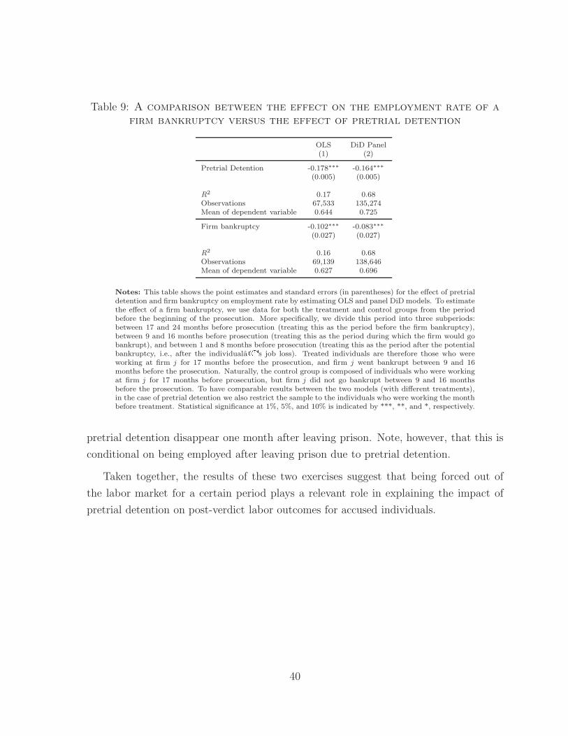
Table 9: A comparison between the effect on the employment rate of afirm bankruptcy versus the effect of pretrial detention

OLS DiD Panel(1) (2)

Pretrial Detention -0.178∗∗∗ -0.164∗∗∗

(0.005) (0.005)

R2 0.17 0.68Observations 67,533 135,274Mean of dependent variable 0.644 0.725

Firm bankruptcy -0.102∗∗∗ -0.083∗∗∗

(0.027) (0.027)

R2 0.16 0.68Observations 69,139 138,646Mean of dependent variable 0.627 0.696

Notes: This table shows the point estimates and standard errors (in parentheses) for the effect of pretrialdetention and firm bankruptcy on employment rate by estimating OLS and panel DiD models. To estimatethe effect of a firm bankruptcy, we use data for both the treatment and control groups from the periodbefore the beginning of the prosecution. More specifically, we divide this period into three subperiods:between 17 and 24 months before prosecution (treating this as the period before the firm bankruptcy),between 9 and 16 months before prosecution (treating this as the period during which the firm would gobankrupt), and between 1 and 8 months before prosecution (treating this as the period after the potentialbankruptcy, i.e., after the individuala€™s job loss). Treated individuals are therefore those who wereworking at firm j for 17 months before the prosecution, and firm j went bankrupt between 9 and 16months before the prosecution. Naturally, the control group is composed of individuals who were workingat firm j for 17 months before prosecution, but firm j did not go bankrupt between 9 and 16 monthsbefore the prosecution. To have comparable results between the two models (with different treatments),in the case of pretrial detention we also restrict the sample to the individuals who were working the monthbefore treatment. Statistical significance at 1%, 5%, and 10% is indicated by ***, **, and *, respectively.

pretrial detention disappear one month after leaving prison. Note, however, that this is

conditional on being employed after leaving prison due to pretrial detention.

Taken together, the results of these two exercises suggest that being forced out of

the labor market for a certain period plays a relevant role in explaining the impact of

pretrial detention on post-verdict labor outcomes for accused individuals.

40

Table 10: A comparison between the effect on monthly wages of a firmbankruptcy versus the effect of pretrial detention

OLS DiD Panel(1) (2)

Pretrial Detention -66,900∗∗∗ -54,222∗∗∗

(2,373) (2,497)

R2 0.58 0.87Observations 67,533 135,274Mean of dependent variable 259,100 275,451

Firm bankruptcy -29,386∗∗ -13,227(12,417) (15,192)

R2 0.54 0.86Observations 69,139 138,646Mean of dependent variable 238,968 253,750

Notes: This table shows the point estimates and standard errors (in parentheses) for the effect of pretrialdetention and firm bankruptcy on average monthly wages by estimating OLS and panel DiD models.To estimate the effect of a firm bankruptcy we use data for both the treatment and control group fromthe period before the beginning of the prosecution. More specifically, we divide this period into threesubperiods: between 17 and 24 months before prosecution (treating this as the period before the firmbankruptcy), between 9 and 16 months before prosecution (treating this as the period during which thefirm would go bankrupt), and between 1 and 8 months before prosecution (treating this as the period afterthe potential bankruptcy, i.e., after the individuala€™s job loss). Treated individuals are therefore thosewho where working at firm j for 17 months before prosecution, and firm j went bankrupt between 9 and 16months before the prosecution. Naturally, the control group is composed by individuals who where workingat firm j for 17 months before prosecution, and firm j did not go bankrupt between 9 and 16 months beforethe prosecution. To have comparable results between the two models (with different treatments) in thecase of pretrial detention we also restrict the sample to the individuals who were working the month beforetreatment. Statistical significance at 1%, 5%, and 10% is indicated by ***, **, and *, respectively.

41

Figure 10: Probability of Retaining Previous Employment after PretrialDetention

0.20

0.40

0.60

0.80

Fra

ctio

n ke

epin

g th

e jo

b of

the

last

mon

th

−10 −9 −8 −7 −6 −5 −4 −3 −2 −1 0 1 2 3 4 5 6 7 8 9 10

Months before the beginning of prosecution and after the final verdict

Treated

Control

Notes: This figure shows the probability of remaining employed at the same firm as the previous month, for the controland treatment groups. Thus, it is only calculated for those individuals who were working the previous month. When thehorizontal axis is negative it represents the months before the beginning of the prosecution, and when the horizontal axisis positive it represents the months after the final verdict. When the horizontal axis equals zero it refers to a period thatis a different length for different individuals, lasting from the beginning of prosecution to the end of trial, including thefinal verdict. The values of the dots in period “1” is equal to the probability of retaining employment in the same firm asthe one in which the individual was employed one month before the beginning of prosecution.

42

6.2 The relevance of the social stigma hypothesis

We do not have data that allows us to directly test the relevance of social stigma mech-

anism hypothesis; however, using our database we can empirically test whether being

prosecuted (without pretrial detention) has some direct effect on labor market outcomes.

Because both the control and treatment groups are prosecuted, this exercise by defini-

tion cannot explain the effect of pretrial detention on labor outcomes. It is, however, an

indirect way to study whether the social stigma that may arise because of prosecution

(or incarceration) plays a relevant role in the determination of labor outcomes.

The nature of our data means that we can only test the effect of prosecution using

our control group sample because it is only individuals in the control group who face

a pure effect of prosecution on labor outcome, as they are not incarcerated during the

prosecution. This pure effect is what can be attributed to social stigma. Therefore, by

construction and because the treatment group is not included in this exercise, the result

cannot explain the differences in outcomes between control and treatment groups that

we find due to pretrial detention.

That said, we study the impact of the start of the criminal prosecution on the em-

ployment rate and average monthly wages for the control group. As stated, we focus on

control group because we want to isolate the effect of positive or negative signals relating

to criminal culpability from the effect of being incarcerated. This is not possible if we

consider individuals who spent time in prison due to a pretrial detention. Panel (a) in

Figure 11 presents the employment rate for the months before and after the beginning of

the prosecution. It shows a reduction of between 4 pp and 5 pp in the employment rate

right after the prosecution begins. Likewise, panel (b) in Figure 11 presents the average

monthly wage for the months before and after the beginning of the prosecution. This

panel shows that there is a reduction of about 7, 000 CLP in the average monthly wage

immediately after the prosecution begins. Given that in these two cases incarceration

was not a factor, it is reasonable to attribute the observed effects to factors that are

specific to a criminal prosecution, and probably to the stigma related with being accused

of a crime, rather than a forced absence from the labor market.

43

Figure 11: Impact of Judicial Decisions on Employment Rate (Pre- andpost-prosecution beginning)

(a) Employment rate

0.42

0.44

0.46

0.48

0.50

Em

ploy

men

t rat

e

−5 −4 −3 −2 −1 0 1 2 3 4 5

Months before and after the beginning of trial

(b) Monthly wages

165,000

170,000

175,000

Ave

rage

wag

e

−5 −4 −3 −2 −1 0 1 2 3 4 5

Months before and after the beginning of prosecution

Notes: These figures show the effect of the beginning of the prosecution (panel a) and the final trial verdict (panel b) onthe probability of being employed. These probabilities are only calculated for the control group. When the horizontal axisis negative, it represents the months before the beginning of the prosecution (panel a) or the months before the final trialverdict (panel b), and when the horizontal axis is positive, it represents the months after the beginning of prosecution(panel a) or the months after the final trial verdict (panel b).

6.3 The relevance of the labor incapacitation hypothesis

As shown in Dobbie et al. (2018) , Leslie and Pope (2017), and Stevenson (2018), pretrial

detention may increase the probability of a guilty sentence. This mechanism may explain

our results to the extent that pretrial detention can lead to post-verdict incarceration

meaning a higher proportion of the treated group, relative to the control group, are

unable to participate in a post-verdict labor market.

We therefore examine whether pretrial detention increases the probability of being

given a custodial sentence, focusing on a Chilean context. Because we cannot implement

the DiD approach in this case (as the dependent variable does not have a pretreatment

value) and given the validity of our IV model, we address this question by estimating

an IV linear model, where the dependent variable is an indicator function that takes

the value of one when there is a custodial sentence, the endogenous variable is pretrial

detention, and the instrument is the judge severity score.

The results of this exercise are presented in Table 11. As the table shows, our

estimates are in line with previous literature in the sense that pretrial detention increases

44

the probability of being given a custodial sentence, although the estimation of the effect

of pretrial detention is not statistically significant (the p-value is 0.167). Regarding the

magnitude, pretrial detention increases the probability of a custodial sentence by 32 pp.

This very large magnitude suggests that the reason our estimates are not statistically

significant is because of statistical power.

Table 11: The impact of pretrial detention on custodial sentence

Custodial sanction

Pretrial detention 0.323(0.234)

Male -0.016**(0.006)

non-Chilean citizen -0.004(0.023)

Indigenous 0.020(0.021)

Crimes special laws 0.030**(0.012)

Drug law crimes 0.216***(0.008)

Homicides 0.197***(0.026)

Nonviolent thefts 0.150***(0.007)

Sex crimes 0.128***(0.008)

Thefts 0.132***(0.029)

Constant -0.338(0.370)

Observations 68,940Court-by-time fixed effects Yes

Notes: This table reports the results for a 2SLS model that estimates the effectof pretrial detention on the probability of a final verdict that results in a custodialsentence. The instrumental variable used in this estimation procedure is the judgeseverity score described in Section 4.2. Robust standard errors are clustered at thejudge level in parentheses. Statistical significance at 1%, 5%, and 10% is indicatedby ***, **, and *, respectively.

Overall, the discussion on the possible explanations for our results suggests that all

three mechanisms may play a role. This is consistent with the results shown in Figures

8 and 9. On the one hand, the effect of pretrial detention on labor outcomes increases

with the amount of time spent incarcerated. If the social stigma due to incarceration and

increase in the probability of a custodial sentence were the only relevant mechanisms,

the actual time of incarceration would be less important. On the other hand, even in

the cases of individuals who only spend a few days incarcerated due to pretrial detention

45

(remember the first tercile spends an average of 296 days in pretrial detention), the effect

of pretrial detention on labor outcomes has a relevant magnitude and is statistically

significant. If stigma and the increase in the probability of a custodial sentence were not

factors, then the effect of a few days of pretrial detention should be close to zero.

7 Conclusion

Pretrial detention may have a negative impact on many dimensions – psychological, socio-

emotional, and economic – for both the individual and for society. Indeed, Ahumada

et al. (2010) showed that the fiscal cost of pretrial detention in Chile in 2007 was 92.48

million USD. In this paper, we contribute to this discussion by estimating the negative

impact of pretrial detention on labor market outcomes. One important limitation of

our analysis is that – due to data limitations – we need to restrict our sample to those

individuals who (pre-arrest) worked in the private formal sector.

The effects found on the employment rate and on average monthly wages are con-

siderable and they last for at least two years, which is the maximum horizon we can

study given our empirical strategy and data. Regarding mechanisms, our results suggest

that the negative effect of pretrial detention is (at least) driven by the lasting effect of

being absent from the labor market during the trial, the social stigma related to being

accused of a crime, and the impact of pretrial detention on the probability of post-verdict

incarceration.

A comprehensive evaluation of the impact that pretrial detention has on society is a

highly complex endeavor that is beyond the scope of this paper. Because the justification

of pretrial detention is generally to protect the criminal investigation and trial, and be-

cause society values these outcomes, the evidence presented in this paper is not enough

to conclude that pretrial detention should not exist. There may very well be a benefit

to society, related to pretrial detention protecting the progress of the criminal investi-

gation, for example. Accordingly, one step further towards a comprehensive evaluation

of pretrial detention would be to estimate the effect of eliminating pretrial detention on

the investigative and prosecution processes.19

19An interesting take in this regard is the study of the impact of alternative precautionary measures,undertaken by Di Tella and Schargrodsky (2013).

46

That said, the large negative impact of pretrial detention that we find in this paper,

which exists even for those who are eventually found innocent or whose crimes are not

deemed worthy of a custodial sentence, invites us to consider two possible paths to

facilitate further progress. On the one hand, we need better evidence on the real benefits

of pretrial detention in order to compare these benefits with the costs identified in this

paper. Only then can we make a judgment on whether the increase in the pretrial

detention rate that we observed over the last decade is justified. On the other hand, we

need to formulate effective policies that attenuate the negative effect on pretrial detention

on post-verdict labor market outcomes. In this regard, our findings suggest that both

the control and treatment groups keep the same labor dynamics pre- and posttrial if they

return to work immediately after the conclusion of the trial (see Figure 10).20 A possible

avenue to attenuate the negative effect of pretrial detention on labor outcomes, therefore,

would be to design public policies that support access to the labor market and finding

an employment position immediately following the conclusion of trial proceedings. 21

20This is in line with Engelhardt (2010) who points out the relevance of the duration of the job searchafter being released from prison. Also see Rauma and Berk (1987), who points out the relevance ofpost-prison unemployment insurance as a way to reduce the probability of recidivism.

21Visher and Kachnowski (2007) show that employment before prison, participation in job trainingduring prison, strong family relationships, and few health problems are associated with finding employ-ment after release.

47

References

Acevedo, G., P. Eskenazi, and C. Pages (2010): “Unemployment insurance in

Chile: A new model of income support for unemployment workers,” Sp discussion

paper, No.0612 World Bank.

Ahumada, A., D. Farren, and B. Williamson (2010): “Los costos de la prision

preventiva en Chile,” Report, Fundacion Paz Ciudanda.

Aizer, A. and J. Doyle, Joseph J. (2015): “ Juvenile Incarceration, Human Capital,

and Future Crime: Evidence from Randomly Assigned Judges,” The Quarterly Journal

of Economics, 130, 759–803.

Apel, R. and G. Sweeten (2014): “The Impact of Incarceration on Employment

during the Transition to Adulthood,” Social Problems, 57, 448–479.

Bald, A., E. Chyn, J. S. Hastings, and M. Machelett (2019): “The Causal

Impact of Removing Children from Abusive and Neglectful Homes,” Working Paper

25419, National Bureau of Economic Research.

Bhuller, M., G. B. Dahl, K. V. LA¸ken, and M. Mogstad (2020): “Incarcera-

tion, Recidivism, and Employment,” Journal of Political Economy, 128, 1269–1324.

Blanco, R., R. Hutt, and H. Rojas (2004): “Reform to the Criminal Justice System

in Chile: Evaluation and Challenges,” Loyola University Chicago International Law

Review, 2, 253–269.

Bushway, S. D. (2004): “Labor Market Effects of Permitting Employer Access to

Criminal History Records,” Journal of Contemporary Criminal Justice, 20, 276–291.

Cortes, T., N. Grau, and J. Rivera (2019): “Juvenile Incarceration and Adult

Recidivism,” Working Papers wp482, University of Chile, Department of Economics.

Dahl, G. B., A. R. Kostol, and M. Mogstad (2014): “ Family Welfare Cultures,”

The Quarterly Journal of Economics, 129, 1711–1752.

Di Tella, R. and E. Schargrodsky (2013): “Criminal Recidivism after Prison and

Electronic Monitoring,” Journal of Political Economy, 121, 28–73.

48

Dobbie, W., J. Goldin, and C. S. Yang (2018): “The Effects of Pretrial Detention

on Conviction, Future Crime, and Employment: Evidence from Randomly Assigned

Judges,” American Economic Review, 108, 201–40.

Duflo, E. (2001): “Schooling and Labor Market Consequences of School Construction

in Indonesia: Evidence from an Unusual Policy Experiment,” American Economic

Review, 91, 795–813.

Engelhardt, B. (2010): “The Effect of Employment Frictions on Crime,” Journal of

Labor Economics, 28, 677–718.

Ferraz, C. and B. Ribeiro (2019): “Pretrial Detention and Rearrest: Evidence from

Brazil,” Working paper.

Finlay, K. (2009): Effect of Employer Access to Criminal History Data on the Labor

Market Outcomes of Ex-Offenders and Non-Offenders, University of Chicago Press,

89–125.

Green, D. P. and D. Winik (2010): “Using random judge assignments to estimate

the effects of incarceration and probation on recidivism among drug offenders,” Crim-

inology, 48, 357–387.

Grogger, J. (1995): “The Effect of Arrests on the Employment and Earnings of Young

Men,” The Quarterly Journal of Economics, 110, 51–71.

Harding, D. J., J. D. Morenoff, A. P. Nguyen, and S. D. Bushway (2018):

“Imprisonment and Labor Market Outcomes: Evidence from a Natural Experiment,”

American Journal of Sociology, 124, 49–110.

Heckman, J. J., H. Ichimura, and P. E. Todd (1997): “Matching as an Econo-

metric Evaluation Estimator: Evidence from Evaluating a Job Training Programme,”

The Review of Economic Studies, 64, 605–654.

Imbens, G. and J. Angrist (1994): “Identification and estimation of local average

treatment effects,” Econometrica, 62, 467–475.

49

Jung, H. (2011): “Increase in the length of incarceration and the subsequent labor

market outcomes: Evidence from men released from Illinois state prisons,” Journal of

Policy Analysis and Management, 30, 499–533.

Kahn-Lang, A. and K. Lang (2019): “The Promise and Pitfalls of Differences-

in-Differences: Reflections on 16 and Pregnant and Other Applications,” Journal of

Business & Economic Statistics, 0, 1–14.

Kling, J. R. (2006): “Incarceration Length, Employment, and Earnings,” American

Economic Review, 96, 863–876.

Knepper, M. (2018): “When the Shadow Is the Substance: Judge Gender and the

Outcomes of Workplace Sex Discrimination Cases,” Journal of Labor Economics, 36,

623–664.

Kolesar, M., R. Chetty, J. Friedman, E. Glaeser, and G. W. Imbens (2015):

“Identification and inference with many invalid instruments,” Journal of Business &

Economic Statistics, 33, 474–484.

Lalonde, R. J. and R. M. Cho (2008): “The Impact of Incarceration in State Prison

on the Employment Prospects of Women,” Journal of Quantitative Criminology, 24,

243–265.

Landersø, R. (2015): “Does Incarceration Length Affect Labor Market Outcomes?”

The Journal of Law and Economics, 58, 205–234.

Leslie, E. and N. G. Pope (2017): “The Unintended Impact of Pretrial Detention on

Case Outcomes: Evidence from New York City Arraignments,” The Journal of Law

and Economics, 60, 529–557.

Loeffler, C. E. (2018): “Pre-Imprisonment Employment Drops: Another Instance of

the Ashenfelter Dip?” Journal of Criminal Law and Criminology, 108, 815.

Mesters, G., V. van der Geest, and C. Bijleveld (2016): “Crime, Employment

and Social Welfare: An Individual-Level Study on Disadvantaged Males,” Journal of

Quantitative Criminology, 32, 159–190.

50

Mueller-Smith, M. (2015): “The Criminal and Labor Market Impacts of Incarcera-

tion,” Working paper, University of Michigan.

Nagin, D. and J. Waldfogel (1995): “The effects of criminality and conviction on

the labor market status of young British offenders,” International Review of Law and

Economics, 15, 109 – 126.

Open Society Fundations (2011): “The Socioeconomic Impact of Pretrial Deten-

tion,” Report, Open Society Justicy Initiative, UNDP.

——— (2014): “Presumption of Guilt: The Global Overuse of Pretrial Detention,”

Report, Open Society Justicy Initiative, UNDP.

Pager, D. (2003): “The Mark of a Criminal Record,” American Journal of Sociology,

108, 937–975.

Pettit, B. and C. J. Lyons (2007): Status and the Stigma of Incarceration: The

Labor-Market Effects of Incarceration, by Race, Class, and Criminal Involvement, Rus-

sell Sage Foundation, 203–226.

Ramakers, A., R. Apel, P. Nieuwbeerta, A. Dirkzwager, and

J. Van Weilsem (2014): “Imprisonment length and post-prison emplyment

prospect,” Criminology, 52, 399–427.

Raphael, S. (2007): The Price of Independence: The Economics of Early Adulthood,

New York: Russell Sage Foundation, chap. Early Incarceration Spells and the Transi-

tion to Adulthood, 278–306.

Rauma, D. and R. A. Berk (1987): “Remuneration and recidivism: The long-

term impact of unemployment compensation on ex-offenders,” Journal of Quantitative

Criminology, 3, 3–27.

Riego, C. and M. Duce (2011): La prision preventiva en Chile, Ediciones de la

Universidad Diego Portales.

Stevenson, M. T. (2018): “Distortion of Justice: How the Inability to Pay Bail Affects

Case Outcomes,” The Journal of Law, Economics, and Organization, 34, 511–542.

51

Stock, J. H., J. H. Wright, and M. Yogo (2002): “A survey of weak instruments

and weak identification in generalized method of moments,” Journal of Business &

Economic Statistics, 20, 518–529.

Visher, C. A. and V. Kachnowski (2007): Finding Work on the Outside: Results

from the “Returning Home” Project in Chicago, Russell Sage Foundation, 80–114.

Walmsley, R. (2016): “World Pre-trial/Remand Imprisonment List (third edition),”

Report, International Centre For Prison Studies Univ. of Essex.

Weiman, D. F., M. A. Stoll, and S. Bushway (2007): The Regime of Mass

Incarceration: A Labor-Market Perspective, Russell Sage Foundation, 29–79.

Western, B. (2006): Punishment and Inequality in America, Russell Sage Foundation.

——— (2007): The Penal System and the Labor Market, Russell Sage Foundation, 335–

360.

Western, B., J. R. Kling, and D. F. Weiman (2001): “The Labor Market Con-

sequences of Incarceration,” Crime & Delinquency, 47, 410–427.

52

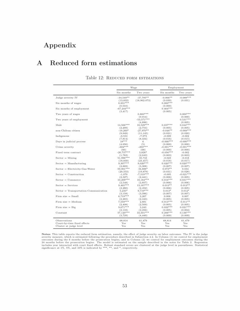
Appendix

A Reduced form estimations

Table 12: Reduced form estimations

Wage Employment

Six months Two years Six months Two years

Judge severity IV -34,549** -37,795** -0.066** -0.088***(13,832) (18,962.073) (0.030) (0.031)

Six months of wages 0.831*** 0.000***(0.010) (0.000)

Six months of employment -67,244*** 0.464***(3,417) (0.005)

Two years of wages 0.883*** 0.000***(0.014) (0.000)

Two years of employment -53,571*** 0.531***(4,896) (0.005)

Male 14,566*** 18,529*** 0.037*** 0.044***(2,209) (2,754) (0.005) (0.005)

non-Chilean citizen -19,260* -27,970** -0.046** -0.068***(9,949) (11,145) (0.021) (0.020)

Indigenous -9,553 -7,973 -0.009 -0.002(7,814) (8,434) (0.016) (0.015)

Days in judicial process 18*** 6 -0.000*** -0.000***(4.656) (5) (0.000) (0.000)

Crime severity -602*** -293*** -0.001*** -0.001***(60) (68) (0.000) (0.000)

Fixed term contract -20,737*** 3,826* -0.056*** -0.002(1,783) (2,043) (0.003) (0.003)

Sector = Mining 51,996*** 35,743 -0.023 -0.018(18,830) (23,457) (0.018) (0.017)

Sector = Manufacturing 9,307*** 9,020*** 0.020*** 0.020***(2,869) (3,308) (0.007) (0.007)

Sector = Electricity-Gas-Water 59,901*** 34,888* 0.073** 0.034(20,553) (19,879) (0.031) (0.028)

Sector = Construction -1,079 -7,519*** -0.005 -0.021***(2,327) (2,441) (0.006) (0.005)

Sector = Commerce 10,209*** 18,184*** 0.016*** 0.031***(2,548) (2,857) (0.006) (0.006)

Sector = Services 9,465*** 13,167*** 0.012** 0.012**(2,280) (2,452) (0.006) (0.005)

Sector = Transportation-Communication 5,235* 9,719*** 0.013* 0.012*(3,158) (3,396) (0.007) (0.007)

Firm size = Small 6,719*** 3,267 0.008 0.007(2,265) (2,443) (0.005) (0.005)

Firm size = Medium 7,559*** 2,881 0.013*** 0.011**(2,408) (2,509) (0.005) (0.005)

Firm size = Big 9,671*** 3,243 0.022*** 0.021***(2,133) (2,256) (0.005) (0.004)

Constant 57,120*** 33,501*** 0.206*** 0.136***(3,729) (4,449) (0.009) (0.009)

Observations 68,814 61,479 68,814 61,479Court-by-time fixed effects Yes Yes Yes YesCluster at judge level Yes Yes Yes Yes

Notes: This table reports the reduced form estimation, namely, the effect of judge severity on labor outcomes. The IV is the judgeseverity measure, which is estimated following the procedure described in Subsection 4.2. In Column (1) we control for employmentoutcomes during the 6 months before the prosecution begins, and in Column (2) we control for employment outcomes during the24 months before the prosecution begins. The model is estimated on the sample described in the notes for Table 2. Regressionincludes year interacted with court fixed effects. Robust standard errors are clustered at the judge level in parentheses. Statisticalsignificance at 1%, 5%, and 10% is indicated by ***, **, and *, respectively.

53

B Monotonicity test

54

Tab

le13:Monotonicitytest

:First

-stageest

imationsfordifferentcrim

etypes

PanelA:First-Sta

geImpactofJudgeseverity,by

Crim

e

Speciallaws

Again

stpublicfaith

Nonviolentth

efts

Sex

crim

es

Dru

glaw

Hom

icid

es&

Thefts

Judgese

verity

IV0.092**

0.457***

0.375***

0.437***

0.184***

0.730***

(0.047)

(0.076)

(0.081)

(0.126)

(0.061)

(0.106)

Obse

rvations

9,725

11,365

11,540

5,822

17,550

12,938

PanelB:First-Sta

geImpactofJudgeseverity,by

Reverse

Sample

Calculation

forCrim

es

Speciallaws

Again

stpublicfaith

Nonviolentth

efts

Sex

crim

es

Dru

glaw

Hom

icid

es&

Thefts

Judgese

verity

IV0.072*

0.420***

0.203**

0.422***

0.160***

0.717***

(0.042)

(0.072)

(0.086)

(0.124)

(0.058)

(0.118)

Obse

rvations

9,721

11,364

11,535

5,822

17,549

12,936

Notes:In

panelA,th

ista

ble

reportsfirst-stage

resu

ltsforth

elinearIV

modelth

atestim

ate

sth

eeffectofpre

trialdete

ntion

on

labor

outc

om

es

by

crim

ese

verity.

PanelB

shows

the

estim

ationsofth

efirst-stage

models,where

the

leave-o

ut

instru

mentis

recalculate

dfordiff

ere

ntsu

bgro

upsusing

all

case

soutsid

eofth

ese

subgro

ups.

The

regre

ssions

inboth

panels

are

estim

ate

dusing

the

sam

ple

as

desc

ribed

inth

enote

sofTable

2.There

gre

ssionsin

clu

deyearin

tera

cte

dwith

court

fixed

effects.Robust

standard

errors

clu

stere

dat

theju

dgelevelin

pare

nth

ese

s.Sta

tisticalsignifi

canceat1%

,5%

,and

10%

isin

dicate

dby

***,**,and

*,re

spectively.

55

C Estimations considering individuals specific’ lin-

ear trends

Table 14: Panel DiD estimations considering individuals specific’ linear trends

Wages Employment

Six months Two years Six months Two years

Petrial Detention -21,827∗∗∗ -24,489∗∗∗ -0.078∗∗∗ -0.089∗∗∗

(1,255) (851) (0.003) (0.002)

R2 0.73 0.61 0.52 0.36Observations 1,712,148 6,664,425 1,712,148 6,664,425Mean of dependent variable 158,321 166,121 0.437 0.440

Notes: This table present the estimations (by panel DiD) for the effect of pretrial detentionon employment and monthly wages, considering individuals specific’ linear trends. The re-gressions are estimated using the sample as described in the notes of Table 2. The regressionsinclude year interacted with court fixed effects. Robust standard errors clustered at the judgelevel in parentheses. Statistical significance at 1%, 5%, and 10% is indicated by ***, **, and*, respectively.

D Robustness analysis: alternative specifications

D.1 Other Differences-in-differences models

In this subsection we present two other DiD models, the cross-sectional DiD model and

the DiD matching model. The cross sectional DiD model, with set of covariates denoted

by Xcsit , considers the same set of control variables as the OLS, except that the year and

month dummies are set at the beginning of the prosecution when t = 0 and at the time

of the sentence when t = 1. The estimated model is given by:

Yi,t = α0+α1PreTriali+α21[t = 1]+βcsPreTriali∗1[t = 1]+γ′Xcsit +ǫit, t ∈ {0, 1}. (8)

The DiD matching is an approach proposed by Heckman et al. (1997), which com-

bines the matching estimation technique with the advantages of the panel DiD estima-

tor. Let Yi,t(PreTriali) denote the potential outcome of individual i at time t, and

∆Yi,t(PreTriali) = Yi,1(PreTriali)−Yi,0 denote the potential increment in the outcome

56

Y between time t = 0 and t = 1. The average treatment effect (ATE) is therefore defined

as βm = E[∆Yi,t(1)−∆Yi,t(0)].

For individuals who were treated we only observe ∆Yi,t(1) = Yi,1 − Yi,0, and we

impute ∆Yi,t(0) using the matching procedure. More specifically, for each i treated

(PreTriali = 1), we assign the set of matches JG(i) corresponding to the G nearest

neighbors in the untreated group (PreTriali = 0) using the Mahalanobis metric, given

the following covariates (Xmit ): gender, Chilean, and indigenous dummies, pretreatment

average wage and employment rate (using 27 to 36 months before prosecution), location

of the court (by region), type of prosecuted crime, and year and month of the sentence.

We report estimates for G = 3. The imputed value for ∆Yi,t(0), denoted by ∆Y i,t(0),

is the average difference outcome of those individuals in the set of matches, that is

∆Y i,t(0) =1G

∑j∈JG(i) ∆Yj,t. Similarly, we can also assign to each untreated individual i

(PreTriali = 0) the set of G nearest neighbors in the treated group JG(i). In this case,

we observe ∆Yi,t(0) = Yi,1−Yi,0 and impute ∆Y i,t(1) =1G

∑j∈JG(i) ∆Yj,t. In this setting,

an estimate of the ATE is:

βm =1

N1 +N0

( ∑

i:PreTriali=1

∆Yi,t(1)− ∆Y i,t(0) +∑

i:PreTriali=0

∆Y i,t(1)−∆Yi,t(0)

),

(9)

where N1 =∑

i:PreTriali=1 1 is the total number of treated individuals, and N0 =∑i:PreTriali=0 1 is the total number of non-treated individuals.

Because the DiD matching procedure finds controls by minimizing the distance among

individuals’ observables, to the extent that these observables explain why some individ-

uals are treated and other are not, this approach has the advantage that it can be more

robust to the existence of time trends for different outcomes, which are function on these

observables – namely, if these observables have specific effect on the time trend of the

outcome, this is going to be properly controlled by the approach. In other words, a DiD

matching approach can be thought as a non-parametric approach to control for time

trends that are functions of observables.

The results from these two approaches (the cross-sectional DiD and DiD matching

models) are presented in Tables 15 (for employment rate) and 16 (for average monthly

wages). To facilitate a comparison with the main results, we also include the point

57

estimates from the panel DiD (also reported in Tables 7 and 8). As these tables show,

the point estimates are very stable across different DiD models.

Table 15: Effect of pretrial detention on employment rate (differentDiD models)

Cross-Section Panel Matching(1) (2) (3)

Six months of employment

Petrial Detention -0.099∗∗∗ -0.098∗∗∗ -0.082∗∗∗

(0.004) (0.003) (0.003)

R2 0.14 0.76 .Observations 284,838 285,358 142,418Mean of dependent variable 0.465 0.465 0.437

Two years of employment

Petrial Detention -0.089∗∗∗ -0.085∗∗∗ -0.079∗∗∗

(0.003) (0.003) (0.003)

R2 0.26 0.75 .Observations 253,094 253,550 126,546Mean of dependent variable 0.464 0.463 0.441

Notes: This table presents the results for the impact of pretrial detention on employment rate,considering different DiD models (using the sample described at Table 2). The results are presentedfor two time horizons: the average for the six months after the final trial verdict and the averagefor the two years after the final trial verdict. Column (1) presents the cross sectional DiD model,Column (2) presents the panel DiD model, and Column (3) presents the results from the DiDmatching model. The mean of the dependent variable is calculated by only considering the controlgroup. Statistical significance at 1%, 5%, and 10% is indicated by ***, **, and *, respectively.

58

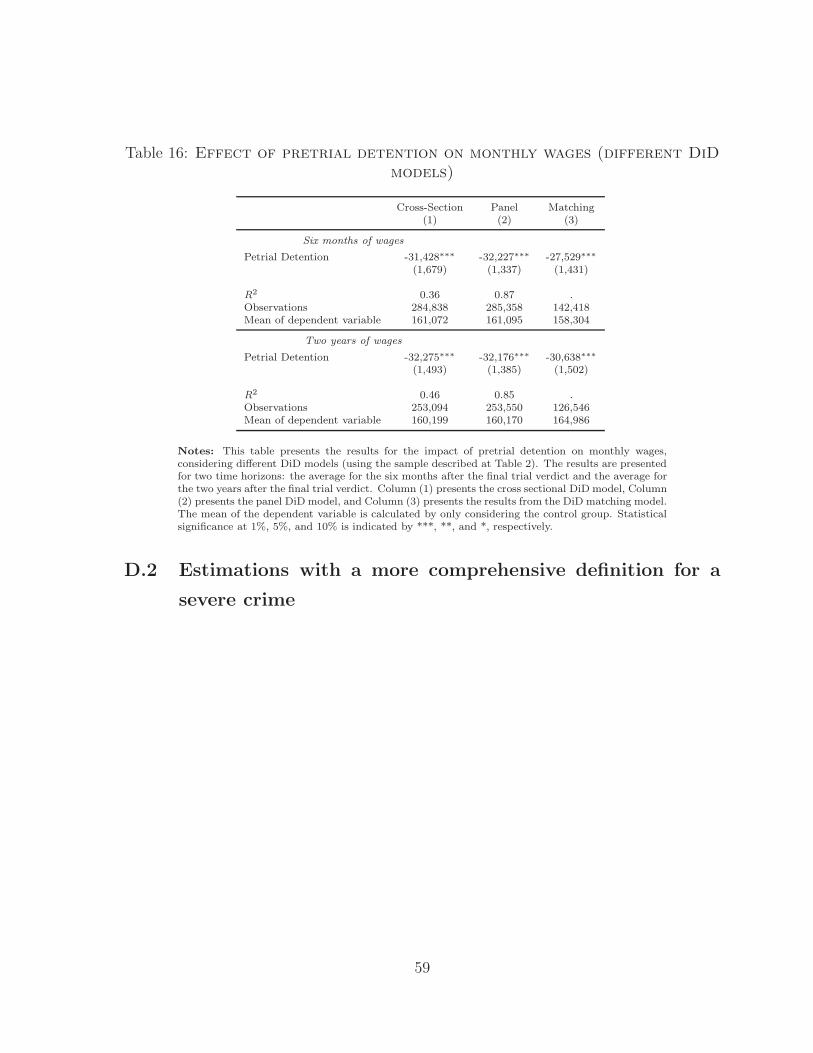
Table 16: Effect of pretrial detention on monthly wages (different DiDmodels)

Cross-Section Panel Matching(1) (2) (3)

Six months of wages

Petrial Detention -31,428∗∗∗ -32,227∗∗∗ -27,529∗∗∗

(1,679) (1,337) (1,431)

R2 0.36 0.87 .Observations 284,838 285,358 142,418Mean of dependent variable 161,072 161,095 158,304

Two years of wages

Petrial Detention -32,275∗∗∗ -32,176∗∗∗ -30,638∗∗∗

(1,493) (1,385) (1,502)

R2 0.46 0.85 .Observations 253,094 253,550 126,546Mean of dependent variable 160,199 160,170 164,986

Notes: This table presents the results for the impact of pretrial detention on monthly wages,considering different DiD models (using the sample described at Table 2). The results are presentedfor two time horizons: the average for the six months after the final trial verdict and the average forthe two years after the final trial verdict. Column (1) presents the cross sectional DiD model, Column(2) presents the panel DiD model, and Column (3) presents the results from the DiD matching model.The mean of the dependent variable is calculated by only considering the control group. Statisticalsignificance at 1%, 5%, and 10% is indicated by ***, **, and *, respectively.

D.2 Estimations with a more comprehensive definition for a

severe crime

59

Table 17: Effect of pretrial detention on employment rate (with thethreshold for severe crime at 5% detained pretrial)

OLS DiD Panel IV(1) (2) (3)

Six months of employment

Petrial Detention -0.127∗∗∗ -0.108∗∗∗ -0.341∗∗∗

(0.003) (0.003) (0.125)

R2 0.31 0.77 0.31Observations 171,268 343,168 82,574Mean of dependent variable 0.473 0.498 0.489

Two years of employment

Petrial Detention -0.118∗∗∗ -0.093∗∗∗ -0.318∗∗∗

(0.003) (0.003) (0.116)

R2 0.29 0.75 0.27Observations 151,469 303,486 73,305Mean of dependent variable 0.474 0.492 0.490

Notes: This table presents the results for the impact of pretrial detention on employment rate,considering the panel DiD and the IV models (using a larger sample where a severe crime isdefined as one where 5% of cases receive pretrial detention). The results are presented for twotime horizons: the average for the six months after final trial verdict and the average for thetwo years after final trial verdict. In order to group the results of a number of specificationsin one table, we only present the point estimates and standard errors (in parentheses) forthe parameter of interest. Column (1) presents the OLS results (Eq. 1), which is a usefulreference point. Column (2) presents the panel DiD model (Eq. 2), and Column (3) presentsthe results from the IV model (Eq. 6). The mean of the dependent variable is calculated byonly considering the control group. Statistical significance at 1%, 5%, and 10% is indicated by***, **, and *, respectively.

60

Table 18: Effect of pretrial detention on monthly wages (with thethreshold for severe crime at 5% detained pretrial)

OLS DiD Panel IV(1) (2) (3)

Six months of wages

Petrial Detention -46,230∗∗∗ -36,841∗∗∗ -160,078∗∗∗

(1,323) (1486) (57,575)

R2 0.58 0.88 0.59Observations 171,268 343,168 82,574Mean of dependent variable 177,861 179,963 185,440

Two years of wages

Petrial Detention -45,788∗∗∗ -37,478∗∗∗ -192,334∗∗∗

(1,354) (1540) (69,131)

R2 0.53 0.86 0.53Observations 151,469 303,486 73,305Mean of dependent variable 183,519 176,957 191,941

Notes: This table presents the results for the impact of pretrial detention on average monthlywages, considering the panel DiD and the IV models (using a larger sample where a severe crimeis defined as one where 5% of cases receive pretrial detention). The results are presented for twotime horizons: the average for the six months after final trial verdict and the average for the twoyears after verdict. In order to group the results of a number of specifications in one table, weonly present the point estimates and standard errors (in parentheses) for the parameter of interest.Column (1) presents the OLS results (Eq. 1), which is a useful reference point. Column (2)presents the panel DiD model (Eq. 2), and Column (3) presents the results from the IV model(Eq. 6). The mean of the dependent variable is calculated by only considering the control group.Statistical significance at 1%, 5%, and 10% is indicated by ***, **, and *, respectively.

61

D.3 Estimations with the IV sample

Table 19: Effect of pretrial detention on employment rate (IVestimation sample)

OLS DiD Panel IV(1) (2) (3)

Six months of employment

Petrial Detention -0.120∗∗∗ -0.093∗∗∗ -0.178∗∗

(0.004) (0.004) (0.084)

R2 0.32 0.77 0.32Observations 68,814 137,628 68,814Mean of dependent variable 0.450 0.478 0.450

Two years of employment

Petrial Detention -0.113∗∗∗ -0.082∗∗∗ -0.210∗∗∗

(0.004) (0.004) (0.075)

R2 0.29 0.76 0.29Observations 61,479 122,958 61,479Mean of dependent variable 0.455 0.475 0.455

Notes: This table presents the results for the impact of pretrial detention on employment rate,considering the panel DiD model (using the IV estimation sample). The results are presentedfor two time horizons: the average for the six months after final trial verdict and the averagefor the two years after verdict. In order to group the results of a number of specifications inone table, we only presented the point estimates and standard errors (in parentheses) for theparameter of interest. Column (1) presents the OLS results (Eq. 1), which is a useful referencepoint. Column (2) presents the panel DiD model (Eq. 2), and Column (3) presents the resultsfrom the IV model (Eq. 6). These column estimates are, by construction, the same as in Table7 (Column (3)). The mean of the dependent variable is calculated only considering the controlgroup. Statistical significance at 1%, 5%, and 10% is indicated by ***, **, and *, respectively.

62

Table 20: Effect of pretrial detention on monthly wages (IV estimationsample)

OLS DiD Panel IV(1) (2) (3)

Six months of wages

Petrial Detention -41,536∗∗∗ -30,492∗∗∗ -92,635∗∗

(1,724) (1958) (38,019)

R2 0.58 0.88 0.58Observations 68,814 137,628 68,814Mean of dependent variable 163,293 166,178 163,293

Two years of wages

Petrial Detention -40,537∗∗∗ -31,087∗∗∗ -90,647∗∗

(1,849) (2055) (46,093)

R2 0.52 0.85 0.52Observations 61,479 122,958 61,479Mean of dependent variable 170,560 165,170 170,560

Notes: This table presents the results for the impact of pretrial detention on average monthlywages, considering the panel DiD model (using the IV estimation sample). The results arepresented for two time horizons: the average for the six months after the final trial verdict andthe average for the two years after the final trial verdict. In order to group the results of anumber of specifications in one table, we only present the point estimates and standard errors(in parentheses) for the parameter of interest. Column (1) presents the OLS results (Eq. 1),which is useful as a reference point. Column (2) presents the panel DiD model (Eq. 2), andColumn (3) presents the results from the IV model (Eq. 6). This column estimates are, byconstruction, the same as in Table 8 (Column (3)). The mean of the dependent variable iscalculated by only considering the control group. Statistical significance at 1%, 5%, and 10% isindicated by ***, **, and *, respectively.

E The impact of pretrial detention for accused indi-

viduals who were released after verdict

E.1 Potential Selection Bias

If we focus our attention on cases where the verdict was not guilty or a non-custodial

sentence was passed, and given the fact that our treatment may affect this status, we

need to investigate to what extent selection bias could be an issue in this empirical

setting.

To discuss potential selection bias, we use equation (2) but add two elements to the

analysis. First, we allow for the fact that the effect of pretrial detention is heterogeneous

across individuals (βi), such that βi = β + ei. Second, we introduce a selection equation

Ii = 1[θ0 + θ1PreTriali − I∗i > 0], where Ii is a binary variable that takes the value

63

of one if the verdict is not guilty or a non-custodial sentence is passed (i.e., i belongs

to our estimation sample) or zero otherwise. And I∗i is a continuous variable, which

is unobservable by the econometrician, that measures all the information that judges

have to support their decision regarding whether or not to detain the individual pretrial.

Note that this selection equation allows for the fact that pretrial detention decreases the

probability of being part of our estimation sample (θ1 < 0), conditional on I∗i . Combining

these new elements with equation 2, we have:

E[Yit|ωi, Xit, P reTriali, t, Ii = 1] = α1[t = 1] + βP reTriali ∗ 1[t = 1] + γ′Xit + ωi

(10)

+ E[ǫit|ωi, Xit, P reTriali, t, Ii = 1] + PreTriali ∗ 1[t = 1]E[ei|ωi, Xit, P reTriali, t, Ii = 1],

In this context, the unobserved component of the selection equation can be related to

the principal equation in two ways.22 In a first structure for the unobserved components,

we allow that I∗i 6⊥⊥ ǫit (and I∗i ⊥⊥eit). In this case E[ǫit|ωi, Xit, P reTriali, t, Ii = 1] 6= 0

and can be written as H(Pretriali) where H is an unknown function. Note, however,

that in this context, equation (10) can be rewritten as:

E[Yit|ωi, Xit, P reTriali, t, Ii = 1] = α1[t = 1] + βP reTriali ∗ 1[t = 1] + γ′Xit + ωi,

where ωi = ωi +H(Pretriali). Therefore, this structure for the unobserved components

does not generate an identification issue in the context of the panel DiD model. It does,

however, generate an endogeneity issue if we estimate β using an IV approach, as in

equation (6), a specification that only uses the cross-sectional nature of the database.23

In a second structure for the unobserved components, we allow that I∗i 6⊥⊥ eit (but

22We are assuming that – conditional on fixed effects – the only source of endogeneity is the selectionbias – namely E[ǫit|ωi, Xit, P reT riali, t] = 0. Moreover, without loss of generality, we make the followingnormalization: E[ei|ωi, Xit, P reT riali, t] = 0, which means that β is the ATE of pretrial detention forthe full sample (i.e., i|Ii = 0 or Ii = 1).

23If a selection bias did exist, it would bias our results toward to zero, given that those who are notpart of the treatment group because they were sentenced to prison are probably already less likely to beemployed or to have a high salary. Hence, this selection process would artificially increase the averagemonthly wage and the employment rate of the treatment group.

64

I∗i ⊥⊥ǫit), in this case E[eit|ωi, Xit, P reTriali, t, Ii = 1] 6= 0. Given this structure, equation

(10) can be written as:

E[Yit|ωi, Xit, P reTriali, t, Ii = 1] = α1[t = 1] + (β + E[eit|Ii = 1])PreTriali ∗ 1[t = 1]

+ γ′Xit + ωi,

Note that here we also do not have an endogeneity issue, but we must be careful in

the interpretation of our estimate. In particular, we must interpret our point estimates

of β as the average treatment effect for those individuals who are part of our estimation

sample (i|Ii = 1). Accordingly, this second structure for unobserved components only

has consequences for the external validity of our results.

In sum, and considering all the elements we have discussed, we think that our best

specifications to estimate the effect of pretrial detention on labor outcomes are the lon-

gitudinal difference-in-differences specifications.

E.2 Estimations

Table 21: Effect of pretrial detention on employment rate (samplemembers released after final trial verdict)

Six months of employment Two years of employment

Petrial Detention -0.054∗∗∗ -0.044∗∗∗

(0.005) (0.004)

R2 0.77 0.76Observations 180,178 158,942Mean of dependent variable 0.500 0.497

Notes: This table presents the results for the impact of pretrial detention on employment rate, considering thepanel DiD approach, using the sample described in Table 2 but further restricting the sample to accused individualswho were released after the final trial verdict. The results are presented for two time horizons: the average for thesix months after the final trial verdict and the average for the two years after the final trial verdict. The mean ofthe dependent variable is calculated only considering the control group. Statistical significance at 1%, 5%, and 10%is indicated by ***, **, and *, respectively.

65

Table 22: Effect of pretrial detention on average wage (sample membersreleased after final trial verdict)

Six months of wages Two years of wages

Petrial Detention -20,772∗∗∗ -20,392∗∗∗

(2,271) (2,406)

R2 0.88 0.86Observations 180,178 158,942Mean of dependent variable 184,103 182,402

Notes: This table presents the results for the impact of pretrial detention on average monthly wages,considering the panel DiD approach, using the sample described at Table 2 but further restricting thesample to accused individuals who were released after the final trial verdict. The results are presentedfor two time horizons: the average for the six months after the final trail verdict and the average forthe two years after final trial verdict. Statistical significance at 1%, 5%, and 10% is indicated by ***,**, and *, respectively.

66