The effects of economic integration on regional growth, anevolutionary model

by

M.C.J. Caniëls (TUE) and B. Verspagen (ECIS and MERIT)

October 1999

AbstractThis paper will present a multi-region-multi-country model in which inter-regional knowledgespillovers determine the growth of regions. Key parameters in the model are the learningcapability of a region, and the exogenous rate of knowledge generation (R&D). The intensityof spillovers depends on geographical distance between regions. The model is investigated bymeans of simulation techniques. What results is a core-periphery situation, the exact form ofwhich depends on the assumed spatial structure. One surprising result of the analysis is thatlarger technological differences between regions may lead to smaller disparity in terms of thelong-run spatial distribution of GDP per capita.

The impact of economic integration is investigated by comparing two different aspects ofthe model. First, examining a fixed exchange rate system versus a system of flexible exchangerates results in conditions (constellations of parameters) under which fixed exchange rates(compared to flexible exchange rates) generate less disparity across regions. However,depending on the parameter values, fixed exchange rates may also generate more disparity,leading to the conclusion that the effect of monetary integration is ambiguous.

Second, the impact of barriers to knowledge spillovers is analysed by assuming that crossborder knowledge flows are hampered compared to inter-country flows. This results in theobservation that reduced cross border flows have a large impact when regions are initiallyunequal with respect to their exogenous rate of knowledge generation or their learningcapability. In these cases, the resulting trends in overall disparity are quite different from thetrends established in a situation of no barriers to knowledge spillovers.

1

1. IntroductionThe issue of convergence of GDP per capita is the topic of a large and growing literature ineconomics (e.g., Barro and Sala-i-Martin, 1995, Fagerberg, 1994). The general conclusionfrom this literature is that convergence, as opposed to divergence, is a special outcome thatmay prevail between a set of countries that is relatively homogenous in terms of variablessuch as knowledge generation (R&D), infrastructure, educational systems, etc. This idea isimplicit in the notion of ‘conditional convergence’ that arises from new growth models in theneoclassical tradition (e.g., Barro and Sala-i-Martin, 1995), as well as in the so-calledtechnology gap theory (e.g., Fagerberg, 1994).

Economic integration, for example in the form that has been implemented in the EuropeanUnion, may well help to achieve homogeneity between countries with regard to the abovementioned structural characteristics, and thus help to achieve convergence (e.g., Ben-David,1994). However, the empirical evidence on convergence of GDP per capita among Europeanregions seems to point out that such convergence is not, or in the best case at very low speed,taking place at the regional level in the Union at large since the start of the 1980s (Fagerberg,Verspagen and Caniëls, 1997).

This paper suggests that the impact of spatial proximity on the diffusion of technologicalknowledge may be responsible for this paradoxical situation. There is a large literature ineconomic geography that underlines the importance of proximity for knowledge spillovers.The concept of interest in this literature (for an overview see Baptista, 1998) is the existenceof agglomeration economies and its effects on growth. Agglomeration economics involve thepositive effects on a firm or a region generated by a spatial concentration of economicactivity. Agglomeration economies are induced, among others, by a large opportunity forcommunication of ideas and experience, which is enhanced by spatial proximity. In this paperwe focus on knowledge spillovers as the prime form of agglomeration economies. Severalstudies (e.g., Acs, Audretsch and Feldman, 1992, Jaffe, Trajtenberg and Henderson, 1993)have confirmed such a positive relation between geographic proximity and knowledgespillovers.

Theoretical reasons for the localized nature of knowledge spillovers are as follows.Technological knowledge is often informal, tacit and uncodified in its nature (e.g., Pavitt,1987). This implies that there are differences between knowledge and information, where theformer concept is more far-reaching than the latter. Audretsch and Feldman (1996) argue thatalthough the cost of transmitting information may be invariant to distance, presumably thecost of transmitting knowledge rises with distance. Possibilities for learning-by-doing andlearning-by-using, important for the transmission of knowledge, to a large extent come fromdirect contacts with competitors, customers, suppliers and providers of services (Von Hippel,1988, 1994) and are therefore highly dependent on proximity.

Uncertainty is another characteristic of the innovative process. Interaction betweeninnovators, e.g. in regional networks, helps to reduce this uncertainty. This kind of interactionis highly dependent on geographical proximity. In this respect, Freeman (1991) points out thatnetworks frequently tend to be localised. Another reason why proximity has an effect on theinnovative process lies in the fact that innovation relies heavily upon sources of basic

2

scientific knowledge. Jaffe (1989) and Acs, Audretsch and Feldman (1992) have empiricallyshown that knowledge spillovers from university research to private firms are facilitated bygeographic proximity. Furthermore, innovative activity is cumulative, meaning that newinnovations build upon scientific knowledge generated by previous innovations. Breschi(1995) and Malerba and Orsenigo (1995) point out that the accumulation of innovativeactivity in a geographic area facilitates the generation of new innovations in this area.

In this paper we incorporate spatial proximity into a technology gap growth modeldeveloped earlier by Verspagen (1991). The resulting model, which is discussed in greaterdetail in Caniëls (1999) is one in which a multitude of geographic units (which will be calledregions) interact with each other in terms of knowledge diffusion. These regions may differwith respect to their R&D efforts and their social capability to assimilate knowledge fromother regions. Ceteris paribus, knowledge from regions close by diffuses more easily thanknowledge from regions far away.

Barriers to trade and barriers to knowledge spillovers can have an important influence onthe distribution of growth across regions. First, trade can have an influence on growth, byenhancing specialisation and thus enabling increasing returns to scale. Various trade-growthmodels explore this relation (Grossman and Helpman, 1990). Second, internationalspecialisation may have an impact on the amount of spillovers that take place within a countryrelative to the amount between countries. Thus, barriers to trade and to knowledge spilloversmay well have an influence on the distribution of gaps throughout all regions.

To be able to study these influences, the situation under barriers to trade and knowledgespillovers is compared to a situation in which these barriers are released. In other words,comparing a situation before and after these two forms of economic integration will make itpossible to explore the effects of trade barriers on the distribution of growth.

It is difficult to make a clear-cut distinction between barriers to trade and barriers toknowledge spillovers. International barriers to trade come in various formats. Exchange ratevolatility, quota’s, tariffs and a political unstable situation all form barriers to internationaltrade. Under the (Millian) assumption that trade in goods is accompanied by diffusion ofknowledge (every product contains information about for instance its construction that can bededuced by reverse engineering) a barrier to cross country trade can limit the knowledgespillovers in these directions. However, trade is one (indirect) way in which knowledge isdiffused.

The aim of this paper is to explore the effects of trade barriers and barriers to knowledgespillovers on regional disparities in growth. The model developed in this paper will take intoaccount increasing returns, through the Verdoorn effect. Specialisation will not beendeepened as a source of disparity across regions, since only one sector will be introduced.

The rest of this paper is organised as follows. In Section 2, the part of the model thatdescribes technological spillovers across regions is presented. Section 3 extends the model toa multi-country setup. Section 4 examines the effect of trade barriers on the model bycomparing a fixed exchange rate system to a system of flexible exchange rates by means ofsimulation techniques. The effect of barriers to knowledge spillovers are analysed in Section5. Finally, Section 6 summarises the main conclusions from this paper.

3

2. Description of the spillover systemFor simplicity, we disregard any sources of output growth other than the growth oftechnological knowledge. Specifically, it is assumed that output growth is a linear function ofthe growth of the knowledge stock:

KK =

Q

Q

i

i

i

i��

β ,

(1)in which Qi denotes the level of output of region i and Ki points to the level of the knowledge

stock of region i. β is a parameter, indicating the proportion of the knowledge stock growththat results in output growth. Dots above variables denote time derivatives.

New knowledge is assumed to stem from three sources: learning-by-doing (modelled as aVerdoorn effect1), spillovers received from surrounding (not necessarily contingent) regions

(Si), and an exogenous rate of growth (ρi), which can be thought of as reflecting the impact ofexogenous R&D activities in the region. This yields the following equation:

,) + S + Q

Q ( =

K

Kii

i

i

i

i ρλα��

(2)

in which α and λ are parameters. α points out the extent to which the knowledge stock growth

is influenced by the above factors, and λ reflects the intensity of the Verdoorn effect.For the explanation of the spillover term S, it is convenient to first consider two regions,

later on this framework will be extended, and a multi-region model will be constructed. In thetwo-region setting, it is assumed that there is one technologically advanced region and onebackward region. Spillovers depend on the size of the knowledge gap, as well as threedifferent parameters reflecting distinct effects related to the realisation of potential spillovers.We use the following equation to model spillovers:

,e = S )-G 1

(-

ij

ii

2iij

i

µδγ

δ

(3)

K

K = Gj

iij ln ,

(4)in which Si denotes the spillovers generated by region j and received by region i2. Gij denotesthe technology gap of region i towards region j, and is defined as the log of the ratio of the

1 The Verdoorn-Kaldor law states that a positive relation exists between the growth of productivity and thegrowth of output.2 Note that the lower the initial stock of knowledge a region is endowed with, the more spillovers it will receive.

This is similar to the concept of β-convergence (Barro, 1984; Baumol, 1986; De Long, 1988; Barro and Sala-i-

Martin, 1991, 1992a, 1992b) in which a backward economy (an economy with a low initial level of GDP percapita) will grow faster than a rich economy and therefore catch up.

4

knowledge stocks of two regions. The realisation of the potential spillover level depends on

the three parameters γ, δ and µ, which we will now discuss in turn.

γij is the geographical distance between two regions. If γij increases, the spillover isreduced. This assumption stems from the geographical literature. As was discussed in theintroduction of this paper, this is based on the assumption that spatial proximity easesspillovers (agglomeration economies), because interaction between the receiver and generator

of the spillovers is easier when distance is small. µi and δi are two parameters that are relatedto the intrinsic learning capability of region i. These parameters thus reflect the broad conceptof ‘social capability’ to assimilate spillovers (e.g., Abramovitz, 1994). Regions that have ahigh social capability to learn (e.g., a highly educated workforce, good infrastructure, anefficient financial system, etc.), can implement the knowledge from other regions more easily.

µi and δi reflect different parts of the learning capability that will be explained further bymeans of graphical analysis.

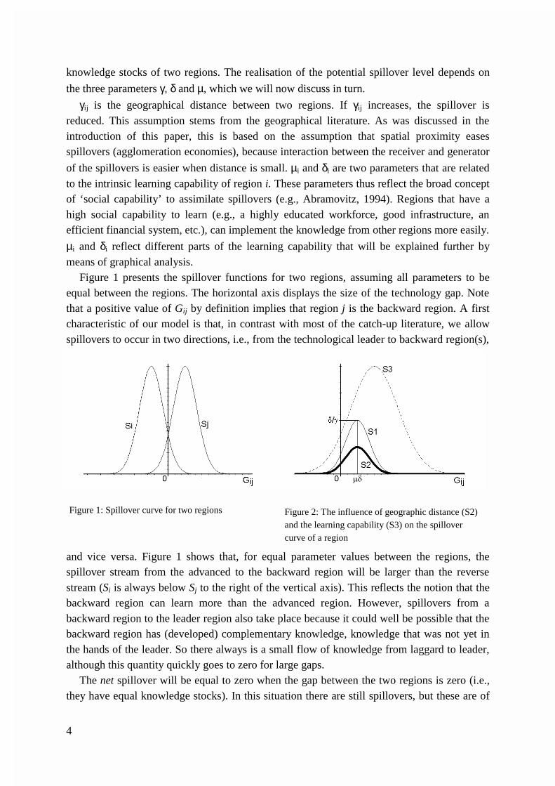
Figure 1 presents the spillover functions for two regions, assuming all parameters to beequal between the regions. The horizontal axis displays the size of the technology gap. Notethat a positive value of Gij by definition implies that region j is the backward region. A firstcharacteristic of our model is that, in contrast with most of the catch-up literature, we allowspillovers to occur in two directions, i.e., from the technological leader to backward region(s),

and vice versa. Figure 1 shows that, for equal parameter values between the regions, thespillover stream from the advanced to the backward region will be larger than the reversestream (Si is always below Sj to the right of the vertical axis). This reflects the notion that thebackward region can learn more than the advanced region. However, spillovers from abackward region to the leader region also take place because it could well be possible that thebackward region has (developed) complementary knowledge, knowledge that was not yet inthe hands of the leader. So there always is a small flow of knowledge from laggard to leader,although this quantity quickly goes to zero for large gaps.

The net spillover will be equal to zero when the gap between the two regions is zero (i.e.,they have equal knowledge stocks). In this situation there are still spillovers, but these are of

Figure 1: Spillover curve for two regions Figure 2: The influence of geographic distance (S2)and the learning capability (S3) on the spillovercurve of a region

5

equal size in both directions. This only holds, however, when the parameters (ρ, λ, µ, δ) areequal between the two regions. In the more general case of unequal parameters betweenregions, net spillovers may be positive or negative for a gap of value zero.

Figure 2 displays the spillovers received by one region for this two-region model. Note that

the top of each spillover curve lies at a technology gap equal to µjδj. The maximal spillover

corresponding to this is equal to δj/γij . We take the curve labelled S1 as the starting point, andwe consider what happens to the spillover function under certain conditions. First, an

enlargement of the geographical distance between two regions (higher γ) will lead to lowerspillovers received by each region, depicted by the thick line S2. Note that an increase indistance shifts the curve down, but leaves the value of the gap for which spillovers aremaximal unchanged.

Second, an increase in the learning capability parameter δ of the lagging region will causethe spillover function to shift up, and the maximum of the curve to shift to the right (dotted

line S3).3 Thus, with higher δ, the laggard is able to learn more (magnitude of the spilloverfunction) and more easily, or earlier (at a larger technological distance).

As will be explained below, the value of G at which the spillover curve peaks (µδ) isimportant for the result in terms of convergence or divergence. We therefore want to allow for

the possibility that maximum of the spillover curve shifts left or right, without affecting the

value of the maximum itself. Figure 3 shows how the parameter µ does exactly this.

If µj is increased, all other things being equal, the curve will shift to the right (S5). This hasseveral effects. First, the level of spillovers in the case of equal knowledge stocks across

regions (G=0), is smaller. This indicates that for relatively large µ, the model resembles aregular catch-up model, which is characterised by zero spillovers for zero technologicaldistance. Second, because the top of the curve moves to the right, catch-up becomes easier. Ata larger technological distance, it is still possible to catch up. How the distinction betweencatching-up of falling behind works exactly will become clearer after we discuss the netspillover function. 3 To achieve this reaction of the spillover curve, the learning capability had to appear in two places in thespillover function (Equation 3).

Figure 3: The influence of a change in the catch-up

parameter µ on the spillover curve

6

Thus, the difference between the parameters µ and δ is mainly a technical matter. Inpractice, they can hardly be disentangled in terms of the variables that make up social

capability to assimilate spillovers. We mainly use the parameter µ to calibrate the model (i.e.,to generate a setup that implies a reasonable borderline between catching-up and falling-

behind), while δ is used more actively in the simulation experiments below as an indicator ofthe learning capability of a region.

In order to be able to analyse the dynamics of convergence and divergence, we take thetime derivative of the technology gap in Equation (4) and substitute equations (1), (2) and (3).For a two-region model this yields:

1 < < 0 with ,))S-S(-)-(( -1

= K

K-

K

K = K

K dt

d = G ijji

j

j

i

i

j

iij αβλρρ

αβλα��

� ln ,

(5)

in which α, β and λ are assumed to have the same value in each region. This expression canbe analysed using Figure 4.

We will restrict ourselves to describing only one case, namely the one in which region i isthe leader, i.e., where the initial gap is positive. We also assume that leadership implies larger

R&D efforts, such that ρi>ρj.4 In Figure 4, Sj-Si represents the difference in received

spillovers between the two regions. The lagging region receives positive net spillovers, as

discussed above. Note that we have again assumed δi = δj and µi = µj. In the more generalcase where these assumptions do not hold, the net spillover curve will not intersect with the

origin, but this does not change the dynamics in a major way. The horizontal line ρi - ρj

displays the difference in the exogenous rate of growth of the knowledge stock between thetwo regions.

It is straightforward from equation (5) that when the curve in Figure 4 intersects with the

horizontal line ρi - ρj, the time derivative of the technology gap is equal to zero. In otherwords, the intersection points correspond to equilibrium points. The (leftmost) intersection

4 This assumption is not essential. Obviously, the case where region j is the leader is the mirror-image of the casewe discuss.

Figure 4: The dynamics of the model

7

point at which the S-curve has a positive slope is stable, whereas the other intersection pointis unstable. Thus, what happens to the knowledge gap in the long run depends on where theprocess starts. Starting points to the left of E2 will yield convergence to a stable technologygap (corresponding to E1). Starting values to the right of E2 will yield falling behind, with anever growing knowledge gap.5

Now consider what happens with changing parameter values. We will first consider avariation in the difference in the exogenous rate of growth of the knowledge stock between

the two regions, ρi - ρj. If the difference is enlarged in favour of the leader, the ρi - ρj line inFigure 4 moves upward, meaning that the range of technology gaps at which catch-up occurs

becomes smaller. Eventually, when the ρi - ρj line shifts to a position above the net spillovercurve, there will be no opportunity at all for catch-up. If, on the other hand, the exogenousrate of growth of the knowledge stock in the backward region is increased (e.g. by expanding

research efforts) up to a level comparable with the advanced region, i.e., the ρi - ρj lineultimately coincides with the horizontal axis, and the (stable) equilibrium gap is zero,implying complete converge in the long run.

Next, we consider the impact of the geographical distance between the two regions. A

decrease in the geographical distance has the effect that the spillover curves Si and Sj increaseproportionally to the decrease in geographical distance (explained by Figure 2) and themaximum of the Sj-Si curve in Figure 5 moves upwards6. Figure 6 displays the bifurcationdiagram for this case.7 The horizontal axis of the bifurcation diagram shows the values of the

geographical distance parameter γij . The vertical axis shows the equilibrium values of thetechnology gap. The line Esj shows the stable equilibrium, while the line Euj points to theunstable equilibrium. The line Smaxj represents the top of the net spillover curve in Figure 5.

5 Verspagen (1991) estimates a simpler version of this model for a large sample of countries over the post-warperiod, and finds that falling behind is a frequent phenomenon.6 The maximum also moves a little bit away from the y-axis, but this is a very small effect.7 Note that the figure should show a discontinuous graph (in the model a geographical distance is either 1 or 2,not 1.5), however, for visual reasons the individual points are connected.

Figure 5: The impact of geographical distance on thenet spillover curve

Figure 6: Bifurcation with respect to geographicaldistance

8

This figure shows that for high values of γij no equilibrium value of the technology gap exists.In terms of Figure 5, this occurs when there are no intersection points between the curves. For

a threshold value of γij , one equilibrium appears. This occurs when the two curves in Figure 5

are tangent. For values of γij smaller than the threshold level, two equilibria exist, as describedby the curves in the bifurcation diagram.

A similar bifurcation analysis can be performed for the parameter δ. The effect of an

increase in the learning capability of the backward region j (δj) on the Sj-Si curve is displayed

in Figure 7. Note that δj is the only parameter that has changed, δi is kept constant. It canclearly be seen that on the right hand side of the figure the top of the curve has moved to theupper right of the figure and the curve does not intersect with the origin anymore. What hashappened on the left-hand side is a bit more difficult to see. The minimum point has moved

upwards so that it is closer to the horizontal axis. Also, there is a small movement of theminimum point away from the y-axis. The bifurcation diagram now looks as displayed inFigure 8.

Note that the Es line for the stable equilibrium can even go below the x-axis if thedifference in exogenous growth rates of the knowledge stock is small enough, whichillustrates an interesting special case of the model. This situation indicates a take-over inleadership by the (initially) lagging region. In terms of Figure 7, this occurs when the

horizontal line (ρi - ρj) intersects with the Sj-Si curve left from the y-axis, where the gap issmaller than zero, indicating that region j is the leader region. The combination of a largelearning capability in the lagging region together with a small difference in the exogenous rateof growth between laggard and leader gives rise to a take over of the lead position by thebackward region. Note that it is primarily learning capability that drives this process of take-over.

We omit the bifurcation analysis for the µ parameter, which is relatively straightforward,and jump to extend the model to a multi-regional case. Suppose we have a world with k

regions, so that each region can be characterised by k-1 technology gaps (we omit the trivialcase of Gii). Spillovers are received from each of the other regions, so that the S terms in

Figure 8: Bifurcation with respect to the learningcapability

Figure 7: The impact of the learning capability onthe net spillover curve

9

equation (2) now become sums of spillovers over k-1 regions. This gives rise to the followingmodified form of equation (5):

,,

ln

jinand1 < < 0 with

,))S-S(-)S-S(+)-(( -1

= K

K-

K

K = K

K dt

d = G ijjnninnji

j

j

i

i

j

iij

≠

ΣΣ

αβλ

ρραβλα��

�

(5’)

in which ΣnSin and ΣnSjn denote the spillovers received by region i and j respectively from all

regions n for which n ≠ i, j (this term is thus invariant to Gij). Note that equation (5’) specifiesthe (growth of the) gap between the two regions i and j only. There are k regions in total, thusevery region i has k-1 of these equations.

Equation (5’), under the ceteris paribus assumption with respect to the knowledge stocks inregions other than i and j, gives rise to identical figures as Figures 4-8. The only difference is

that in the case of equation (5’), (ρi - ρj) and (ΣnSin - ΣnSjn) are lumped together into the

horizontal lines that used to be determined by (ρi - ρj) only. A movement of this horizontalline (and therefore in the horizontal position of E2) can now be caused by two factors. First, avariation in the difference between the exogenous rates of growth of the knowledge stocks oftwo regions (as before), and, second, a difference across regions in the spillovers receivedfrom all other regions.

The latter term is largely determined by geographic location. The subset of regions towhich this term refers does not differ between i and j, but when, for example, region i iscloser to the advanced regions than region j is, this gives region i an advantage over region j.

Also, the learning capability (δ and µ) has an impact on how (ΣnSin - ΣnSjn) differs between iand j).

3. Extending the model to a multi-country set-upThe economy consists of a number of countries (denoted by j = 1..m), each of which containsseveral regions (denoted by i = 1..nj). Only one good is produced (specialisation is ruled out).Demand for the good is assumed to be determined by the number of people (denoted by N),labour productivity (defined by a = Q/L, in which Q denotes production and L denotes thenumber people who have a job) and the world price in terms of the home currency (eP, edenotes the exchange rate and P the world price) for the good. Increasing labour productivityis assumed to have a positive influence on demand, since it gives an indication of a relativehigh general level of development of the economy. The demand function is given by thefollowing equation:

,Pe

a N d = D

j

ijijijij

(6)in which d is a parameter.

Supply is assumed to be inelastic in the short run, so that it can be set equal to productivecapacity (Q). Capital is homogenous. Assuming a fixed coefficients production technology,

10

labour demand is simply a function of the capital stock in the sector. We assume one worldprice for the good, which can be found by confronting world demand with world supply:

, aNl = P e

a N dijijij

n

1=i

m

1=jj

ijijijn

1=i

m

1=j∑∑∑∑

(7)where the share of total population employed in region i of country j is defined as l ij = Lij/Nij

(L is labour demand, equal to C/(ac), where C is the capital stock, and the capital output ratio

c ≡ C/Q is assumed to be a fixed parameter). When (initial) levels for C, N, a and e are given,this equation can be solved for the world price P as follows:

. L

e

N d

= P

ij

n

1=i

m

1=j

j

ijijn

1=i

m

1=j

∑∑

∑∑

(8)The growth of labour productivity is assumed to be proportional to the growth of theknowledge stock:

K = a ijij ˆˆ ξ ,

(9)

in which ξ is a parameter which is set equal to one in the following experiments. The spilloversystem, as introduced in the former section, determines the knowledge stock of each region ateach moment in time.

Next, we define capital accumulation. The ‘real’ profit rate (profits as a share of the capitalstock) is defined as follows:

,P e a

w - 1

c

1 =

C P e

L w - Q P e = r

jij

ij

ijj

ijijijjij

(10)where w is the nominal wage rate (measured in domestic currency). We assume that all profitsare reinvested in capital in the same region, and that the price for capital equipment is equal tothe world price of output. Thus, the growth rate of the capital stocks can be written as:

.ˆ r = C ij

(11)Now, we add the dynamics of the exchange rates. The value of the trade balance measured

in foreign currency per sector is equal to the difference between the country’s production andits consumption, i.e.:

)D - Q( P = B jjj .

(12)

11

The assumption is that the growth of the exchange rate depends on the value of the tradebalance as a fraction of the value of total GDP (both measured in current prices and foreigncurrency). More specifically, we assume that the following equation holds:

,Q P

B - Q P

B = e *

*

j

jj

εˆ

(13)

where ε (>0) is a parameter. The superscript * indicates the reference country for which thegrowth in the exchange rate is equal to zero, (ê = 0, e = 1). This formulation ensures certainbasic characteristics with regard to consistency. For example, a change of the referencecountry (i.e., expressing all values for all countries in the currency of a different country) doesnot change the growth rates of the exchange rates using the above equation. Also, note thatthe exchange rate between two countries of which neither is the reference country can becalculated by dividing their exchange rates relative to the reference country. Thus, for m

countries, one can calculate all remaining (m2-m)/2 exchange rates if the m exchange ratesrelative to one reference country are known. The above equation for the dynamics of theexchange rate ensures that changing the reference country does not change the resultingvalues of the exchange rate growth rates.

The labour market is characterised by a Phillips curve, determining the growth of thenominal wage rate:

,N

L n + m- = wij

ijˆ

(14)

in which m and n are parameters. Population (N) is assumed to grow at a fixed rate η.When we specify a (symmetric) matrix of distances between regions, the model is fully

specified, and time paths for the G variables result from any set of initial values. However, formore than two regions, these time paths are extremely tedious to work out analytically, whichis why we resort to simulations to describe the outcomes of the model. By carrying out manysimulations (with randomised initial conditions) it is possible to examine the generalbehaviour of the model, and we find that certain patterns in the gaps of the knowledge stocksappear repeatedly. All simulations use a Pascal computer program that implements a Runge-Kutta algorithm to numerically solve the differential equations for G.

We use two different geographical spheres (distance matrices). These are a lattice ofhoneycombs and a globe. Appendix A gives an exact description and a map of these spheresas well as the location of the border which divides each sphere into countries. The regions onthese spheres are assumed to be homogeneous areas. In other words, no differences of therelative importance (e.g., political) of the regions are assumed, nor do we assume differencesin the degree of connectedness (e.g. the presence of harbours, mountains, roads and railways).Since this is a one-sector model, we also assume that the regions have homogenous economicstructures. The first of these spheres is two-dimensional. A honeycomb pattern is chosen inorder to provide an equal amount of contingent neighbours for each region, with each

12

neighbour having an equally long border. This would not be the case when using a lattice ofsquares, which would have the additional difficulty of judging the importance of the differentkinds of neighbours - queens, bishops or rooks8 - by assigning weights to them. Because thelattice is flat and has a hexagonal shape in itself, there is always exactly one central region.This region has a favourable location, as will become clear from the experiments.

The second sphere used has the shape of a globe. In the globe, no inherently centrallocation is present. In the case of the globe pentagons had to be added to the hexagons (theregions are constructed as the pattern on a soccer ball, i.e., 12 pentagons and 20 hexagons)9.The lattice of honeycombs can be considered similar to a country, whereas the globe could bea model for a world.

Geographic distance in the geographical spheres is measured by assigning a weight of 1 toneighbouring regions (in the sense that two regions share one border). Regions which do notshare a border with a specific region are given a weight by using the concept of nearestneighbours, which means that a different (lower) weight is attributed to a second orderneighbour. A second order neighbour does not share a border with a specific region, but doesshare a border with a neighbour of the specific region. In this way, the distance gij isdetermined for every region towards every other region. Now, it is possible to construct a

region-by-region matrix of shortest paths. Then, the corresponding weights (γ) are determinedusing the inverse of the orders (inverse shortest path, Hagett, Cliff and Frey, 1977). Note thatthis way of measuring geographical distance is a special case of 1/(gij

x) with x equal to 1. Next, we will examine the effect of a fixed exchange rate system versus a system of

flexible exchange rates. We focus on the conditions (constellations of parameters) underwhich fixed exchange rates compared to flexible exchange rates generate less disparity acrossregions. Second, the impact of barriers to knowledge spillovers is analysed by assuming thatcross border knowledge flows are hampered compared to inter-country flows.

8 These terms are borrowed from chess. A queen is allowed to move in all directions indicating that all 8neighbours of a square are equally important. A lattice with these characteristics is called a Mooreneighbourhood. A bishop is only allowed to move in a diagonal way, while a rook is only allowed to movehorizontally or vertically, meaning that one might want to assign a different (lower) weight to a neighbours,which do not share a border but only one point (the bishops-case) than to neighbours, which do share a border(the rooks-case). When only neighbours of the rook type are considered, the plain is called a von-Neumannneighbourhood.9 It is impossible to construct a three-dimensional figure by the single use of hexagons. Hexagons will alwaysproduce a flat sphere, since the sum of the angles of three contingent hexagons is equal to 360 degrees. Byadding pentagons, the total angle will be less than 360 and thus producing a three-dimensional figure. It wouldhave been possible to construct a three-dimensional sphere by using pentagons only, however, in that case thetotal number of pentagons (regions) used would be twelve. The globe that is used in the simulations consists ofthirty-two planes (regions), which was considered to give more interesting interactions than a sphere containingonly twelve planes.

13

4. Flexible exchange rates versus fixed exchange ratesIn the recent literature, a discussion takes place about whether economic integration, moreprecisely a monetary union, will have overall positive or negative effects on the growth of theeconomies involved (Flam, 1992).

This section focuses on the introduction of irrevocably fixed exchange rates and the effectsof this on regional growth in our model10. Some general characteristics of the simulations willbe illustrated using the globe. The geographic space of the globe is distributed between twocountries in a way that each country comprises a different amount of regions. The firstcountry contains 9 regions and is therefore labelled as small compared to the second countrywhich consists of the resting 23 regions. Our first simulation experiment assumes that allregions are initially equal, except for their geographic location11. Figure 9 shows thecoefficient of variation (the average over the last 100 periods) over the gaps in GDP per capitain all regions for fifty runs in two cases: flexible exchange rates and a monetary union.

The figure points out several things: first, the disparity under a monetary union is largerthan under flexible exchange rates. This leads to the tentative conclusion that the introductionof a monetary union leads to an increase in the gaps across regions12. Second, the disparityunder a monetary union shows less variability than the disparity under flexible exchangerates. A monetary union therefore leads also to a stabilisation of the outcome.

The question arises whether the monetary union will always cause a higher disparity acrossregions compared to the flexible exchange rate case. What influence do the parameters in themodel have on the distribution of the gaps under a monetary union versus flexible exchangerates? To explore these questions we will address both geographic spaces. Simulations were

generated for several start values of the parameters δ and ρ and the initial level of the

10 The terms ‘monetary union’ and ‘system of fixed exchange rates’ will be used interchangeably, since in termsof the model a system of fixed exchange rates is identical to a monetary union. Both refer to a situation in whicheach currency can be denominated in the currency of another country against a fixed rate.11 The initial values of the data are described in Appendix B. Note that the population varies across runs, but notacross regions.12 The difference in the disparity between flexible exchange rates and a monetary union is quite small in absoluteterms, however, a clear difference is present. Note that the coefficient of variation over the gaps in the labourproductivity is taken, where the gap is defined by a logarithmic function, which suppresses high values.

1.3112

1.31125

1.3113

1.31135

1.3114

1.31145

1.3115

1.31155

1.3116

1.31165

1 4 7 10 13 16 19 22 25 28 31 34 37 40 43 46 49

Flexible exchange rates Monetary union

Figure 9: Overall disparity per run

14

knowledge stock. At the start of each simulation all regions had exactly the same‘endowments’, in the sense that each region has an equal learning capability, level of theknowledge stock, population etc. (Appendix B shows the initial values of all parameters andvariables). Across simulations, the parameters and variables were initially set at a differentlevel. In each constellation, the coefficient of variation was determined in the case of flexibleexchange rates and a monetary union. Figure 10 gives a visual impression of the results forthe lattice of honeycombs. On the horizontal axis the value of the learning capability, whichvaried from 0.5 to 4.5 is denoted. The vertical axis shows the exogenous rate of growth of theknowledge stock that varied in the same interval. A grey cell indicates that the disparity undera monetary union was higher than under flexible exchange rates. The five different panels aremade for five different values of the initial level of the knowledge stock.

Figure 10: Differences in disparity between a monetary union and a system of flexible exchange rates: results forthe lattice of honeycombs

ρ ρ ρ ρ ρ4

3

2

1

1 2 3 4 δ 1 2 3 4 δ 1 2 3 4 δ 1 2 3 4 δ 1 2 3 4 δKnowledge stock =0.5

Knowledge stock =2.5

Knowledge stock =4.5

Knowledge stock =6.5

Knowledge stock =8.5

Several interesting phenomena are illustrated by this figure. First, a clear pattern is shownin the panels. There appear to be zones, which stretch from the upper left to the lower right. Ineach zone, either a monetary union or a system of flexible exchange rates causes moredisparity across regions. The combination of learning capability and exogenous rate of growthof the knowledge stock therefore causes the disparity in the monetary union to be higher orlower than under flexible exchange rates. Second, as the knowledge stock is increased, somechanges occur in the pattern, but these appear to be less systematic. This indicates that achange in the initial level of the knowledge stock has only little influence on whether amonetary union causes more disparity across regions than flexible exchange rates.

Furthermore, Figure 10 shows several cells that do not change colour as the knowledgestock is increased. In general, it is the case that if the knowledge stock has reached a relativelyhigh value (8.5), the cells will not change colour anymore due to a further increase in theinitial level of the knowledge stock. The situation is now stable in that either the monetaryunion or the flexible exchange rates case shows the largest disparity.

This overall result emphasises that under certain combinations of the learning capabilityand the exogenous rate of knowledge generation more disparity might occur as a result of the

15

introduction of a monetary union. This contradicts the general believe that the introduction ofa monetary union will generate convergence across the participation countries/regions.

More precisely, the results indicate that both parameters (the learning capability, δ, and the

exogenous rate of growth of the knowledge stock, ρ) and a variable (the level of theknowledge stock at the start of the simulation) all have an influence on whether a monetaryunion induces a lower or higher disparity across regions than flexible exchange rates. Theinfluence of initial level of the knowledge stock becomes marginal as it reaches a high value.

However, the influence of δ and ρ is much higher. An enlargement of the learning capability

(keeping ρ and the initial level of the knowledge stock equal) will lead to several switches incolour in Figure 10. This indicates that a small change in the learning capability induces anew situation in which either a monetary union or flexible exchange rates cause the highestdisparity across regions. The exogenous rate of growth of the knowledge stock has a less

strong impact. As ρ is increased (all other things equal) there appear large intervals in which amonetary union generates a larger disparity across regions than flexible exchange rates andthe other way around. This might lead to the conclusion that it is easier to use the exogenousrate of growth of the knowledge stock as a policy instrument (for example by increasing theamount of R&D) than influencing the learning capability of all regions. Influencing thelearning capability might lead to overshooting of the objective that the introduction of amonetary union leads to less disparity than would be the case as flexible exchange rates weremaintained.

Figure 11 shows the results for the globe. A clear division appears between the grey andthe white areas. As the knowledge stock is enlarged, the grey area becomes larger. Thus, wefind more constellations in which the disparity caused by a monetary union is larger than thedisparity under flexible exchange rates. We see that from the point that the knowledge stock isequal to 4.5 a grey area emerges at the left-hand side of the panel, reducing the white areafrom left to right.

This figure points out that as the initial level of the knowledge stock is increased acrossregions, the grey area is enlarged, until finally the parameters no longer have an influence on

the direction of the difference. At high values of the knowledge stock, each combination of δand ρ leads to a situation in which a monetary union causes a larger disparity than a system offlexible exchange rates. Applying the globe as the prevailing geographic structure we find thatin many cases (parameter constellations) a monetary union leads to divergence in regionalgrowth. This is a remarkable result, considering the implicit assumption of the EuropeanUnion that integration favours convergence in growth across regions.

16

Figure 11: Differences in disparity between a monetary union and a system of flexible exchange rates: results forthe globe

ρ ρ ρ ρ ρ4

3

2

1

1 2 3 4 1 2 3 4 1 2 3 4 1 2 3 4 1 2 3 4

δ δ δ δ δKnowledge stock =0.5

Knowledge stock =3

Knowledge stock =4.5

Knowledge stock =5.5

Knowledge stock =7

This section illustrated what effects different conditions (constellations of parameters likethe learning capability and the exogenous rate of growth of the knowledge stock) have on thedisparity in the gaps of the knowledge stock across regions. These conditions are explored intwo different stages of integration, namely a system of flexible exchange rates and a monetaryunion. The choice of the geographical sphere has a large impact on the results. The lattice ofhoneycombs might be the most realistic sphere to compare with the European Union. In thissphere, we see that specific combinations of the learning capability and the exogenous rate ofgrowth of the knowledge stock lead to less disparity across regions in the case of a monetaryunion, but other combinations show an adverse effect. This leads to the conclusion that amonetary union does not unambiguously lead to convergence in regional gaps.

5. Barriers to knowledge spilloversThe existence of national systems of innovation stimulates inter-country regional interactionrather than cross border relationships. The experiments in this section aim to explore theeffect of barriers to knowledge spillovers on regional convergence. In this section, a barrier toknowledge spillovers across countries is introduced by reducing the spillovers that cross theborder between the countries with one half. The specific effect of introducing knowledgebarriers to this model is analysed by comparing the results of this experiment to the resultsfound for the situation of no barriers to knowledge spillovers. This is documented in Figures14 and 17. The underlying geographical structure is the lattice of honeycombs.

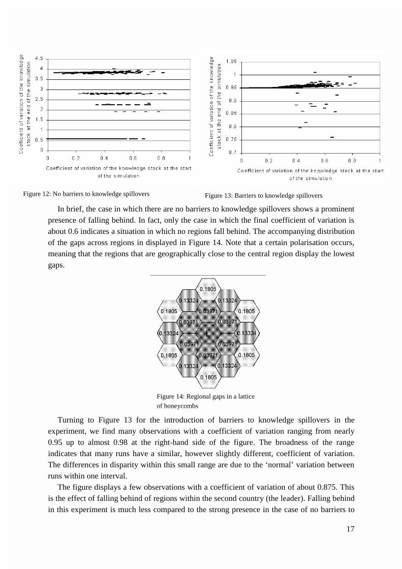
In this experiment, the initial level of the knowledge stock for each region is drawn from auniform distribution, resulting in several different initial distributions of the knowledge stockacross regions. These initial disparities are displayed on the horizontal axis of the figures. Thevertical axis shows the coefficient of variation at the end of the simulation period. Severalthings emerge from comparing Figure 12 to Figure 13.

17

In brief, the case in which there are no barriers to knowledge spillovers shows a prominentpresence of falling behind. In fact, only the case in which the final coefficient of variation isabout 0.6 indicates a situation in which no regions fall behind. The accompanying distributionof the gaps across regions in displayed in Figure 14. Note that a certain polarisation occurs,meaning that the regions that are geographically close to the central region display the lowestgaps.

Turning to Figure 13 for the introduction of barriers to knowledge spillovers in theexperiment, we find many observations with a coefficient of variation ranging from nearly0.95 up to almost 0.98 at the right-hand side of the figure. The broadness of the rangeindicates that many runs have a similar, however slightly different, coefficient of variation.The differences in disparity within this small range are due to the ‘normal’ variation betweenruns within one interval.

The figure displays a few observations with a coefficient of variation of about 0.875. Thisis the effect of falling behind of regions within the second country (the leader). Falling behindin this experiment is much less compared to the strong presence in the case of no barriers to

Figure 13: Barriers to knowledge spilloversFigure 12: No barriers to knowledge spillovers

Figure 14: Regional gaps in a lattice

of honeycombs

18

knowledge spillovers. Falling behind in Figure 13 leads to less final disparity, contrary to thecase of no barriers to knowledge spillovers in which falling behind induced a higher disparityat the end of the simulation. When knowledge spillovers across countries are hampered allregions within the first country will experience a large gap towards the leader region, which islocated in the second country (this will be explored more in detail in Figure 16). When aregion from within country 2 experiences falling behind (due to unfavourable low initialvalues of its knowledge stock), this induces the overall disparity to decline. Since only a smallnumber of runs is subject to falling behind, we can conclude that under barriers to knowledgespillovers, falling behind has less of an impact on the disparity than before.

Another point originates from Figure 13. At the right-hand side, the coefficient of variationis slightly higher than to the left, while this effect is absent from Figure 12. Because the firstcountry receives little spillovers due to the barriers to cross border spillovers, the equilibriumgap (towards every individual region from this country converges) continues to grow duringthe transitory dynamics. At a high initial coefficient of variation (right-hand side of thefigure), large initial differences between regions are present. Apparently, this causes arelatively high variety in equilibrium gaps across regions (of the first country) within a run.Therefore, the overall disparity is higher than in the case where initial differences acrossregions are smaller (left-hand side of the figure).

The two panels in Figure 15 show the effect of barriers to knowledge spillovers as there areinitial variations in the learning capability and the exogenous rate of growth of the knowledgestock, respectively. Both parameters are drawn from a uniform distribution of decreasing size,where the upper boundary is fixed, and the lower boundary is shifted. The horizontal axis ineach panel in Figure 15 shows the lower boundary. The upper boundary was set equal to 2throughout the simulations13. The vertical axis shows the frequency of the coefficient ofvariation of the gaps. The shades in the figures correspond to frequencies over 50 runs, with

13 Appendix B shows the values of all parameters and variables as they are used for each (set of) simulations.

Figure 15, Panel 1: Frequency diagram of thecoefficient of variation at the end of the run.Initial variation in the learning capability

Figure 15, Panel 2: Frequency diagram of thecoefficient of variation at the end of the run.Initial variation in the exogenous rate ofknowledge generation

Lower boundary of uniform distributionLower boundary of uniform distribution

19

complete black corresponding to a frequency of 50 (i.e., all runs). White shades indicate verylow (sometimes zero) frequencies.

The first panel of Figure 15 shows the results for an initial variation in the learningcapability. A comet-shape appears, in which ‘the comet’ (the dark spot at the right of thefigure) leaves two clear trails: a long one coming from the lower left and a shorter trailoriginating from the upper left. This indicates that an increase in initial disparity acrossregions induces two effects. The upper trail suggests higher disparity, however, a strongereffect originates from the lower trail, which suggests smaller disparity across regions. Themore unequal regions are in terms of their learning capability, the more differences indisparity exist across runs.

A similar comet-shape appears when we observe the results for a variation in theexogenous rate of growth of the knowledge stock (Figure 15, Panel 2). Again, there appeartwo trails of which the lower one is longer. Based on this observation, a variation in theexogenous rate of growth of the knowledge stock seems to have a similar influence on thebehaviour of the model than a variation in the learning capability (although the absoluteinfluence differs).

It is interesting to observe the distribution of the gaps (after 1000 simulation periods)across regions in the case that all regions are initially equal, except for their geographic

location (see Figure 16). Thus, δi = δ, µi = µ, and initially all values for G are equal to zero.

The values for the parameters δ and µ remain fixed over the run, while the values for G,

naturally, evolve according to equation (5’). The number within each honeycomb in Figure 16

indicates the size of the gap of the region toward the leader region14. The regions that have alarge gap towards the leader region are white whereas the leader region and regions with avery small gap towards the leader are coloured grey. The thick line demarcates the borderbetween the two countries.

14 Note that these are average values over the last 100 periods in a run.

Figure 16: Final gaps when all regionsare initially equal

20

The pattern shows strong inter-country variation, rather than inter-regional variation. Allregions within a country have identical colours. The origins for this pattern are found in thefirst periods of the run. The second country comprises the region that on a world level has themost favourable geographic location, the central region. This simple fact causes that country 2in the end becomes the leader country. The centrally located region (in the world) will receivemost spillovers in the first periods of the run, only because of its central position. At the sametime the regions of country 1, neighbouring to this central region, undergo a largedisadvantage of the border. Their spillovers from the advanced country 2 are reduced by onehalf. This process is reinforced as the simulation time passes.

A second observation is that in the second country the leader region is located in the mostfavourable geographic position (the central location) within the country. The world-leaderregion is therefore not the ‘overall’ central region in world. The other regions within country2 show gaps which are (line-) symmetrically distributed around the leader region. Thus,within country 2 the ‘usual’ polarisation (as documented in Figure 14) takes place, in thesense that the regions that are geographically close to the central region display the lowestgaps.

Summarising, a variation in one of the parameters (learning capability or exogenous rate ofgrowth of the knowledge stock) suggests that two states appear most often as the initialdifferences across regions increase with respect to one of the two parameters. In one state thedisparity is larger than in the distribution shown by Figure 16, in the other state the disparityin the gaps across regions is smaller. The latter trail is clearest suggesting that initialdifferences in learning capability or exogenous rate of knowledge generation leads to a lowerdisparity across regions.

The sphere used in the last set of simulations is the globe. A variation in the initial stock ofknowledge across regions leads to a disparity in gaps across regions as displayed in Figure 17.Whereas the final disparity of 1.0117 results independent of the initial disparity acrossregions, a few times a lower final coefficient of variation comes about. Similar to the

Figure 17: Initial versus final disparity under barriers to knowledgespill overs, the globe

21

experiment for the lattice of honeycombs this is due to falling behind within the leadercountry.

Panel 1 of Figure 18 shows the disparity in each run for a variation in the learningcapability. A comet-shape occurs, indicating that an increase in initial disparity across regionsinduces not only less disparity across regions at the end of the simulation but could also causemore disparity. The more unequal regions are in terms of their exogenous rate of growth ofthe knowledge stock, the more differences in disparity exist across runs. However, there seemto be (three) different paths along which the coefficient of variation groups (three trails). Onetrail is moving upward from the black cell towards the upper left. A second path stretches outin a slightly downward direction (from right to left). The third trail is horizontal. Panel 2shows the results for a variation in the learning capability. Again, a comet-shape appears,however, no separate trails are distinguished.

In general, the figures for this geographical sphere show similar trends as for the lattice,

although the amount, direction and clarity of the trails (for an initial random variation in δ or

ρ) differs somewhat.The distribution connected to the situation in which regions have the same initial values is

shown by Figure 1915, 16. As before we find a strong inter-country difference. Within theleader country a polarisation occurs (less clear from Figure 19) around the leader region.

This set of experiments sheds light on the effect of barriers to knowledge spillovers on themodel. A striking result is that a clear difference in the average gap between two countriesoccurs. In one country, all regions will tend to an equilibrium in which their gap toward the

15 It might strike as remarkable that Panel 2 shows a lower final coefficient of variation than in Panel 1. This isdue to the fact that learning capability is set equal to 2 in this experiment, while it was set equal to 1 in the firstset of simulations (see Appendix B).16 Note that the geographic structure of country 2 is a-symmetrical. Therefore, it is less easy to see that the leaderregion is centrally located within country 2. The same experiment has been executed for a different, symmetricgeographic structure for both countries. The results with respect to disparity (for all ranges) are similar. The onlyadvantage of a symmetric geographic structure is that it enables us to immediately see the polarisation around thecentral region of the leader country.

Figure 18, Panel 2: Frequency diagram of thecoefficient of variation at the end of the run

Figure 18, Panel 1: Frequency diagram of thecoefficient of variation at the end of the run

Lower boundary of uniform distributionLower boundary of uniform distribution

22

leader region (located in the other country) is very large. The country containing the leaderregion shows polarisation. This result indicates that the ‘adverse’ effect of variety in learningcapability and exogenous rate of growth of the knowledge stock, i.e. more initial varietycausing less final disparity across regions, only holds within a country.

6. Summary and conclusionsThis paper presented a model for knowledge spillovers based on geographical distance as wellas technological distance. The regions in our model receive knowledge spillovers from otherregions, and this enables them to grow rapidly. Our model is similar to some of the modelsfound in the ‘technology gap’ tradition of analysing convergence of GDP per capita.Compared to these models, we add the spatial distance effect on spillovers. The further awayother regions are, the less strong spillovers from these regions are.

In addition, this paper developed a multi-country model, in which inter-regionalknowledge spillovers determine the growth of regions. By simulations we examined the effectof parameters such as the learning capability and the exogenous rate of growth of theknowledge stock on disparity in different situations. First, the effect of barriers to trade wasinvestigated by comparing two different stages of integration. A fixed exchange rate systemversus a system of flexible exchange rates was examined, resulting in conditions(constellations of parameters) under which fixed exchange rates (compared to flexibleexchange rates) generate less disparity across regions. However, depending on the parametervalues, fixed exchange rates may also generate more disparity, leading to the conclusion thatthe effect of monetary integration is ambiguous.

Second, attention was paid to barriers to knowledge spillovers in the sense that crossborder knowledge flows are hampered compared to inter-country flows. This experimentleads to the result that reduced cross border flows have a large implication when regions areinitially unequal with respect to their knowledge stocks, the exogenous rate of knowledgegeneration or the learning capability. The most important result from this last experiment isthat a difference between countries appears in the resulting pattern of per capita gaps. One ofthe two countries contains the leader region and this region is located centrally within thiscountry. All other regions of the leader country are grouped in a hierarchical pattern aroundthe central region. The other country contains regions that have a large gap towards the worldleader region. This indicates that, with limited cross-border spillovers, the ‘adverse’ effect of

Figure 19: Final gaps when all regions are initially equal

23

variety in learning capability and exogenous rate of growth of the knowledge stock, i.e., moreinitial disparity resulting in less final disparity, only holds within a country.

APPENDIX A

Figure A.1 displays the topography of the regions on a lattice of honeycombs. The number within each hexagonwas used to establish the geographical distances between all hexagons. Figure A.2 represents a globe with 12pentagons and 20 hexagons. For the graphical representation, we used the same principle that was applied inmaking a map of the world. Hence, the regions close to the poles look larger as they actually are, while theregions around the equator show their true proportions. At the bottom and at the top are regions 29 and 9. Theseare pentagons, for example region 9 borders to five regions, namely 3, 2, 8, 10 and 11. Regions 29 and 9 are inreality as large as region 1. The graphic representation of a globe has also as a consequence that for exampleregion 3 seems to differ in size from region 6. Again, this is not the case in reality, region 3 is an ordinaryhexagon. The same goes for all the other regions bordering 9 or 29. It should also be noted that region 11 bordersnot only to regions 9, 10, 24, 25 and 12, but also to region 3. In this way, region 12 also borders to regions 3 and4, region 13 has regions 4 and 14 as direct neighbours as well, whereas region 28 also shares a border withregions 14 and 15.

Figure A.2: Two countries on a globeFigure A.1: Two countries on a lattice

of honeycombs

24

APPENDIX BDefault levels of the variables and values of the parameters:

1 (Catch-up parameter, µ)

0.005 (β)

0.005 (α)

1 (Verdoorn parameter, λ)

1 (ζ)0.01 (ε)0.008 (η)3 (c)1 (d)0.8 (m)1 (n)Exchange rate country 1 = 1.14, (exchange rate country 2 = 1)

γ (geographical distance) is constructed with the help of two different types of distance tables, one for each

sphere.

Level of the knowledge stock and values of the parameters in each figure:

ρ =

1

ρ =

2

δ =

2

δ =

1

δ =

4

Kno

wle

dge

sto

ck =

10

ρ ∈

[1

.8,

2.0

]

δ ∈

[1

.8,

2.0

]

Kno

wle

dge

sto

ck ∈ [

0,

2]

δ ∈

[0

.5,

4.0

] st

ep

0.5

ρ ∈

[0

.5,

4.0

] st

ep

0.5

δ ∈

[0

.5,

4.5

] st

ep

0.5

ρ ∈

[0

.5,

4.5

] st

ep

0.5

Tim

e s

imu

late

d =

10

00

0

Tim

e s

imu

late

d =

10

00

Figure 9 x x x xFigure 10 x x xFigure 11 x x xFigure 12 x x x xFigure 13 x x x xFigure 14 x x x xFigure 15(1) x x x xFigure 15(2) x x x xFigure 16 x x x xFigure 17 x x x xFigure 18(1) x x x xFigure 18(2) x x x xFigure 19 x x x x

25

ReferencesAbramovitz, M.A., (1994), ‘The Origins of the Postwar Catch-Up and Convergence Boom’,

in: Fagerberg, J., Verspagen, B. and N. Von Tunzelmann (eds), The Dynamics of Trade,

Technology and Growth, Aldershot: Edward Elgar, pp. 21-52.Acs, Z.J., Audretsch D.B. and M.P. Feldman, (1992), ‘Real effects of academic research:

comment’, American Economic Review, vol. 82(1), pp. 363-367.Audretsch D.B. and M.P. Feldman, (1996), ‘Knowledge spillovers and the geography of

innovation and production’, American Economic Review, vol. 86(3), pp. 630-640.Baptista, R., (1998), ‘Clusters, innovation and growth: a survey of the literature’, in Swann,

P.G.M., (ed.), The dynamics of industrial clustering – international comparisons in

computing and biotechnology, Oxford: Oxford University Press, pp. 13-51.Barro, R.J. and X. Sala-i-Martin, (1991), ‘Convergence across states and regions’, Brooking

Papers Economic Activity, vol. 1, pp. 107-182.Barro, R.J. and X. Sala-i-Martin, (1992a), ‘Convergence’, Journal of Political Economy, vol.

100, pp. 223-251.Barro, R.J. and X. Sala-i-Martin, (1992b), ‘Regional growth and migration: A Japan-United

States comparison’, Journal of the Japanese and International Economies, vol. 6, pp. 312-346.

Barro, R.J. and X. Sala-i-Martin, (1995), Economic growth, New York: McGraw-Hill.Barro, R.J., (1984), Macroeconomics, New York: Wiley.Baumol, W., (1986), ‘Productivity growth, convergence and welfare: What the long-run data

show’, American Economic Review, vol.76, pp. 1072-1085.Ben-David, D., (1994), ‘Income Disparity among Countries and the Effects of Freer Trade’,

in: Pasinetti, L.L. and R.M. Solow, Economic Growth and the Structure of Long-Term

Development, London: St. Martin’s Press, pp. 45-64.Breschi, S., (1995), ‘Spatial patterns of innovation: evidence from patent data’, paper

presented at the workshop on ‘New Research Findings: The Economics of Scientific andTechnological Research in Europe’, Urbino, Italy, 24-25 February 1995.

Caniëls, M.C.J., (1999), Regional Growth Differentials, the Impact of Locally Bounded

Knowledge Spillovers, Maastricht: Datawyse.De Long, J.B., (1988), ‘Productivity growth, convergence and welfare: comment’, American

Economic Review, vol.78, pp. 1138-1159.Fagerberg, J., (1994), ‘Technology and international differences in growth rates’, Journal of

Economic Literature, 32, pp. 1147-1175.Fagerberg, J., Verspagen, B., Caniëls, M.C.J., (1997), ‘Technology, Growth and

Unemployment across European Regions’, Regional Studies, 31, pp. 457-466.Flam, H., (1992), ‘Product markets and 1992: full integration, large gains’, Journal of

Economic Perspectives, vol. 6, pp. 7-31.Freeman, C., (1991), ‘Networks of innovators: a synthesis of research issues’, Research

Policy, vol. 20, pp. 499-514.Grossman, G. and E. Helpman, (1990), ‘Trade, innovation and growth’, American Economic

Review, vol. 80(2), pp. 86-92.

26

Hagett, P., A. D. Cliff and A. Frey, (1977), Locational models, London: Edward Arnold(publishers) Ltd.

Jaffe, A., (1989), ‘Real effects of academic research’, American Economic Review, vol. 79,pp. 957-970.

Jaffe, A., Trajtenberg, M. and R. Henderson, (1993), ‘Geographic localization of knowledgespillovers as evidenced by patent citations’, Quarterly Journal of Economics, vol. 108, pp.577-598.

Malerba, F., and L. Orsenigo, (1995), ‘Schumpeterian patterns of innovation’, Cambridge

Journal of Economics, vol. 19(1), pp. 47-66.Pavitt, K. (1987), On the nature of technology, Brighton: University of Sussex – Science

Policy Research Unit.Verspagen, B., (1991), ‘A new empirical approach to catching up and falling behind’,

Structural Change and Economic Dynamics, vol. 2, pp. 359-380.Von Hippel, E., (1988), The sources of innovation, New York: Oxford University Press.Von Hippel, E., (1994), ‘“Sticky information” and the locus of problem solving: implications

for innovation’, Management Science, vol. 40(3), pp. 429-439.