the effects of fjel-bound chlorine and alkali on corrosion ... archive/files/merge/vol-42... · the...

THE EFFECTS OF FUEL-BOUND CHLORINE AND ALKALI ON CORROSION INITIATION

I

Larry L. Baxter, Hanne P. Nielsenl Sandia National Laboratories Combustion Research Facility

Livermore, CA 94550

ABSTRACT

This investigation explores the effects of fuel-bound chlorine and alkali metals on the initial phases of metal corrosion under conditions typical of superheaters and reheaters in electric power generating boilers. Experiments were conducted with a variety of fuels in an entrained-flow, pilot- scale combustor that simulates conditions found in commercial-scale, pulverized-coal-fired boilers. Temperature-regulated probes simulated superheater tubes and were sized to reproduce similar mechanisms of deposition as are found in commercial systems. Fuels examined include coals with a wide range of chlorine concentrations, biomass fuels, and coals blended with chlorine-containing biomass fuels. Scanning electron micrographs reveal regions of the interfaces of some such probes that show evidence of chloride condensation and subsequent conversion to sulfates. This chemical conversion releases chlorine-containing gases that can facilitate the corrosion of the surface without being consumed. Hypothesized mechanisms for this corrosion have been presented in the literature and are reviewed. The extent to which chlorine-containing materials accumulate on surfaces and subsequently sulfate is shown to depend strongly on the mechanisms of ash deposition and on surface temperature. Interactions between alkali and other ash constituents are shown to effect the extent of alkali deposition and the amount of sulfation. Implications for combustion of chlorinated fuels are discussed.

INTRODUCTION

One of the primary economic drivers of this investigation is the determination of the level of chlorine in coal that can be allowed before corrosion of heat transfer surfaces becomes intolerable and how this level may vary among coals of similar properties but from different seams. In particular, authors have citcd anccdotal evidence that coals from the Illinois region do not cause corrosion problems in boilers to the extent that UK coals with similar clilorinc levels do. The UK has a great many chlorinated coals whereas the most commercially significant chlorinated coal in the US derive from the Herron Basin, largely within Illinois, and represent a fairly small fraction of the overall US coal market. Operational practices relative to chlorine-induced corrosion rely heavily on UK recommendations, where the greatest experience lies. Generally, these practices suggest not firing coals with greater than 0.3% chlorine unless materials and operations are specifically altered to deal with potential corrosion problems'associated with high-chlorine coals.

There have been no direct comparisons of the corrosion behaviors of UK and US coals in the same utility-scale boiler under the same operating conditions. Since such comparisons are both unlikely to occur and are subject to large uncertainty due to the nature of commercial-scale operation, this investigation was commissioned. The objective of this work is to establish fundamental relationships among operating conditions, fuel properties, and corrosion mechanisms that could be used to establish the corrosion potential of fuels.

Sandia National Laboratories is engaged in a series of investigations regarding the role of chlorine in corrosion in power plants. These investigation focus on deposit formation and initiation of corrosion processes. Chlorine-based corrosion is often associated with alkali metals, and COTTO- sion in general is often aggravated by alkali metals with or without chlorine-present. The purpose of this investigation is to establish which corrosion-related species are most likely to form in the gas-phase and on surfaces under typical combustion conditions and to demonstrate how fuel properties influence their formation. This information leads to a postulated mechanism for chlorine- related corrosion and distinguishing characteristics among fuels that may indicate their corrosion potential.

THERMODYNAMIC STABILITY

Early work on this subject indicated that there may be differences in the rates of release of chlorine depending on the origin of the coal. Specifically, coals from the UK were observed to release chlorine slightly earlier in their combustion histories than were US coals of otherwise similar properties. There was some speculation that this could lead to differing corrosion rates or mechanisms, However, in all cases essentially all of the chlorine was released well before the coals completed

' Work completed while visiting Sandia National Laboratorics, Livermore, CA. irom the Technical University of Denmark. Copenhagen.

1091

combustion. Therefore, all of the chlorine would be in the gas phase long before entering the convection passes of commercial boilers, where corrosion is typically of greatest concern. We view it as unlikely that differences in these early release mechanisms could significantly alter the corrosion rates that occur far downstream from where the differences are observed. However, there may be differences in the coals that lead to differing amounts of alkali being released. These may be more closely related to modes of alkali occurrence than to release rates and mechanisms of chlorine. Al- kali metals are clearly implicated in high-temperature corrosion and their most stable gas-phase form is as chlorides at furnace exit gas temperatures.

Table 1 Elemental composition on which equilibrium calculations are based repre- senting an oxidizing, moist environment typical of lower-furnace regions in many coal-fired boilers. There is excess oxygen, carbon and hydrogen for formation of alkali carbonates and hydroxides, but insufficient sulfur or chlorine to react with all of the alkali lo form sulfstes or chlorides.

Element Molar Ratio Element / Total Alkali

C 202 H 850 0 1593 N 5848 S 0.125

CL 0.375 Alkali (Na or K) I

Temperature I'C]

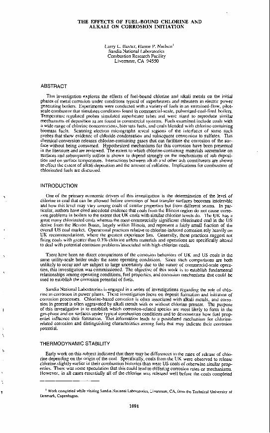
Figure I Equilibrium species coiiceiitratioiis for the major potassium- containing, gas-phase species present under typical coal combustion

Figure 1 through Figure 4 illustrate equilibrium predictions for the major alkali-containing gas- and condensed- phase species as a function of temperature. As illustrated, chlorine and alkali behavior are coupled and this coupling explains some aspects of how ash deposit structure develops. All of the calculations are performed under conditions representative of rumace regions where chlorine is released and char oxidation begins. The molar ratios of each of the atoms relative to the alkali-containing species are indicated in Table I . In general, the oxygen and water mole concentrations in the equilibrium products are about 10%. The molar ratios allow for complete conversion of alkuli to carboiiatcs or hydroxides, but are insufficient to allow coni- plete conversion to either sulfates or chlorides.

conditions. Compare with con- Chlorides represent among the most densed-phase behavior illustrated stable alkali-bearing species in the gas in Figure 2. phase. Chlorine is shown to have a

strong affinity for alkali metal in the temperature ranges of interest to convection pass entrances. In many cases, the amount of alkali vaporized during combustion is determined more by the amount of chlorine available to fonn stable vapors than by the amount of alkali in the fuel I . Figure I illustrates predicted equilibrium concentrations of gas-phase, potassium-containing species under typical coal-combustion conditions. Condensed-phase results are illustrated in Figure 2. Gas-phase sulfate is seen to play a relatively minor role in potassium equilibrium chemistry. Peak sulfate concentrations represent about 10% of the total gas-phase potassium and occur over a narrow temperature range at about 1 100 "C. At lower temperatures, potassium sulfale vapor condenses to form liquid or solid sulfate. At higher temperatures, it decomposes. Thermodynamic predictions of sodium-bearing species are very similar to those of potassium and are illustrated separately in Figure 3 and Figure 4.

The dominant gas-phase, alkali-bearing species at flame temperatures (>I400 "C) is alkali hy- droxide, followed by the chloride. In the absence of significant chlorine for reaction, only the hy- droxide is present. As temperatures cool to convection-pass values (< 1000 "C), hydroxides convert to chlorides, the only alklai-bearing species in significant quantities at lower temperatures. Sulfates are notable by their absence in the gas phase.

..

1092

a

I

F ' ' ' " " '1"' ' " " ' " " " ' ' " I ' 1

- KCI solid - - - K,CO, solid - - - K,SO, sdid A

K,SO, Solid B

80X10*

- - K,SO, liquid

ti Y P 40 a

$ M )

20

0 400 800 1200 1600

TemDeraIure I'CI

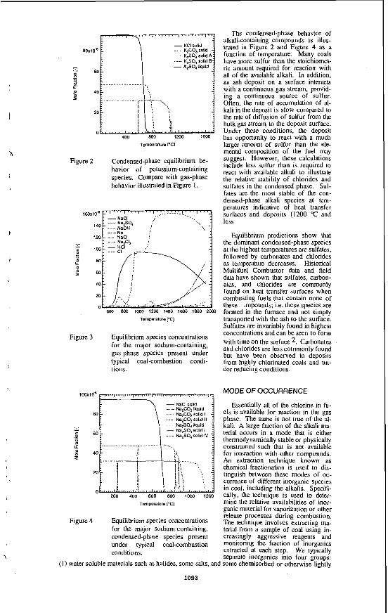
Figure 2 Condensed-phase equilibrium behavior of potassium-containing species. Compare with gas-phase behavior illustrated in Figure 1.

104 . I ' ' I ' * 1 ' ' = I ' ' ' ' ' ,.' ' I ' '1 : -NaCl . ...... Na,SO, :i I4O NaOH < - Na

: Na,C12 ; 120 - - - NaO

600 800 1000 1200 1400 1600 1800 2000

Temperature ['C]

Figure 3 Equilibrium species concentrations for the major sodium-containing, gas-phase species present under typical coal-combustion conditions.

clod

80

60 Na,SO,sotid IV

40

0 200 400 600 800 1000 1200

Temperature ['Cl

Figure 4 Equilibrium species concentrations for the major sodium-containing, condensed-phase species present under typical coal-combustion conditions.

The condensed-phase behavior of alkali-containing compounds is illustrated in Figure 2 and Figure 4 as a function of temperature. Many coals have more sulfur than the stoichiomet- ric amount required for reaction with all of the available alkali. In addition, an ash deposit on a surface interacts with a continuous gas stream, provid- ing a continuous source of sulfur. Often, the rate of accumulation of alkali in the deposit is slow compared to the rate of diffusion of sulfur from the bulk gas stream to the deposit surface. Under these conditions, the deposit has opportunity to react with a much larger amount of sulfur than the elemental composition of the fuel may suggest. However, these calculations include less sulfur than is required to react with available alkali to illustrate the relative stability of chlorides and sulfates in the condensed phase. Sul- fates are the most stable of the condensed-phase alkali species at temperatures indicative of heat transfer surfaces and deposits (1200 "C and less

Equilibrium predictions show that the dominant condensed-phase species at the highest temperatures are sulfates, followed by carbonates and chlorides as temperature decreases. Historical Multifuel Combustor data and field data have shown that sulfates, carbonates, and chlorides are commonly found on heat transfer surfaces when combusting fuels that contain none of these. mpounds; i.e. these species are formed in the furnace and not simply transported with the ash to the surface. Sulfates are invariably found in highest concentrations and can be seen to form with time on the surface 2. Carbonates and chlorides are less commonly found but have been observed in deposits from highly chlorinated coals and 1111- der reducing conditions.

MODE OF OCCURRENCE

Essentially all of the chlorine in fuels is available for reaction in the gas phase. The same is not tme of the alkali. A large fraction of the alkali material occurs in a mode that is either thermodynamically stable or physically constrained such that is not available for interaction with other compounds. An extraction technique known as chemical fractionation is used to dis- tinguish between these modes of occurrence of different inorganic species in coal, including the alkalis. Specifi- cally, the technique is used to determine the relative availabilities of inorganic material for vaporization or other release processes during combustion. The technique involves extracting material from a sample of coal using increasingly aggre'ssive reagents -and monitoring the fraction of inorganics extracted at each step. We typically separate inorganics into four groups:

( I ) water soluble materials such as halides, some salts, and some chemisorbed or otherwise lightly

1093

bound inorganics; (2) ion exchangeable materials such as ions of salts formed from carboxyl and hydroxyl groups in the coal; (3) acid soluble materials such as carbonates and sulfates; and (4) residual materials such as clays and most oxides (silica, titania, etc.).

1 .ca

0.90

0.80

0.70

0.60

0.50

0.40

0.30

0.20

0.10

0.w

oAcld Solubl LI Ion Exchan r Water Solu

LL

Figure 5 Chemical fractionation results for the UK coal indicating the major modes of occurrence for the inorganic components. Compare with Figure 6 .

Results of this procedure are available for representative UK and a US coals with similar chlorine contents. The results indicate that there is ap- proximately 50% more sodium available from the UK coal for participation in the corrosion-inducing reactions indicated above than there is for the US coal. However, the difference arises from the I total sodium content and not from a large difference in the mode of occurrence of the sodium in the fuels. Figure 5 illustrates the results for the UK coal. The fraction of total mass is illustrated for each of the inajor elements in coal. Sodium is of primary interest for corrosion for these fuels. Sodium occurring in mobile forms is more likely to vaporize during combustion than sodium in

the form of clay or other stable compounds. The mobile forms of sodium include the water soluble and ion exchangeable components. The sum of these two forms represents 54% of the sodium in the UK coal and 66% in the Rend Lake coal. This difference is larger than the inherent error in making these measurements (rt 3%), but is probably not significantly larger than the fluctuations in coal properties as delivered from the mine. We find no indication that the modes of occurrence of sodium o r chlorine in these t . 3 samples of fuels would produce significantly different corrosion results. There'are large variations in the mode of occurrence of sodium in coal, and other fuels may show different tendencies. We do anticipate the UK coal would be more corrosive that the US coal in this case, but only because it has a higher overall sodium content. The modes of occurrence of sodium in the two fuels are similar.

Table 2 Chemical fractionation results for the UK coal indicating the major modes of occurrence for the inorganic components on a YO dry fuel basis. Coinpare with Table 3.

SiO, Al,O, TiO, FqO, CaO MgO K,O Na,O P,O, SO, CI

WalerSoluble 0.251 a135 am a016 0.m 0.014 0.m a133 0.011 0.m a017

IonExchangcable a179 LlcB5 0.Cm 0.oLz 0.1% 0.040 O.W 00x1 0.W a073 (1014

AcidSoluble a213 a19 a016 am 0.m 0.031 0.W O.UN 0 . a ~ au18

Residual 7.457 3.553 a m a m a032 0.19 0x6 a121 am a024

Table 3 Chemical fractionation results for the Illinois coal indicating the major modes of occurrence for the inorganic components on a 70 dry fuel basis. Compare with Table 2.

SiO, AI,O, TiO, Fe,O, CaO MgO K,O Na,O P,O, SO, CI

Water Soluble a012 a014 am, 0.081 0.098 a018 am am ami am am IonExchangeable am 0107 a036 0.03 0.lY 0.M9 a011 awl ao3L 0.073 0.m

Acid Soluble 0057 0.oY 0036 am 0.m 0.m am 0.W ami am Residual 3.497 1.614 am 0.814 0.m 0,061 0.166 QMZ 0.015 arm

THE ROLES OF CHLORINE AND ALKALI IN CORROSION

On the basis of these data we postulate the following relationships among operating conditions, boiler design, and fuel properties that impact corrosion. The three fuel properties that most significantly impact rates of corrosion are sulfur, available alkali, and chlorine contents. Corrosion is

1094

strongly influenced by the presence of alkali on the surface of the deposit. This alkali is generally sulfated on the surface, but it appears that the sulfate represents a reaction product from the gas phase and is not, in general, directly deposited. Chlorine enhances corrosion by at least two mechanisms. First, increased chlorine concentrations lead to increased alkali-containing vapors in combustion gases as chlorides are among the most stable alkali-laden species under most combustion conditions. Increased gas-phase alkali concentrations lead to increased rates of alkali deposition on surfaces. Secondly, if the alkali chlorides from the gas phase convert to alkali sulfates on or near heat transfer surfaces, the chlorinated product of the reaction will be concentrated near the heat transfer surface. Chlorine is known to enhance metal corrosion rates significantly under typical superheater conditions. The rate of alkali vaporization and subsequent sulfation can be limited by chlorine, alkali, or sulfur contents. If it is limited by sulfur content, we would expect to see chlorldes on the surfaces of heat transfer equipment. If it is limited by chlorine content or alkali content, chloride content on the surface would be very low even though chlorine plays an important role in both transport of alkali to the surface and corrosion of the metal.

In a series of investigations we have tested es-

Acid Soluble Ion Exchangeable Water Soluble

Figure 6 Chemical fractionation results for the Illinois coal indicating the major modes of Occurrence for the inorganic components. Compare with Figure 5.

literature regarding long-term corrosion

sentially all of the aspects of this conceptual model of chlorine-enhanced corrosion. Alkali vaporization rates increase with increased fuel chlorine content. Alkali sulfates are commonly found concentrated at the metal- deposit interface of probes in the form of sulfates. Chlorides are found on the surface when chlorine levels are increased and sulfur contents are decreased. Figure 7 illustrates a layer of sodium and sulfur found on the surface of a simulated superheater tube during one such investigation. The duration of our tests is insufficient to determine whether these observations can be directly related to long-term corrosion rates, but they are consistent with investigations available in the

Figure 7 SEM image of cross-section of deposits formed on a probe in the Multifuel Combustor. The probe surface is on the left of each image. The images represent the probe surface with deposited pazticles (left), a sodium map (center), and a sulfur map (right).

REFERENCES

I . Baxter, L.L., et al. The Behavior or Inorganic Material in Biomass-Fired Power Boilers -_ Field and Laboratory Experiences: Volunie II of Alkali Deposits Found in Biomass Power Plum Sandia National Laboratories; National Renewable Energy Laboratory, 1996; pp.

Baxter, L.L. I n Sifu, Real-Time Emission FTIR Spectroscopy ar a Diagnostic for Ash Deposition During Coal Combustion ; Engineering Foundation Conference on The Impact of Ash Deposition on Coal-Fired Plants, Solihull, England, 1993; pp.

2.

1095

ANALYSIS OF COMBUSTION PRODUCTS FROM THE COFIRING OF COAL WITH BIOMASS FUELS

Deirdre A. Belle-Oudry and David C. Dayton National Renewable Energy Laboratory

16 I7 Cole Boulevard Golden, CO 80401-3393

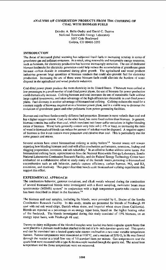
INTRODUCTION The threat of increased global warming has subjected fossil fuels to increasing scrutiny in terms of greenhouse gas and pollutant emissions. As a result, using renewable and sustainable energy resources, such as biomass, for electricity production has become increasingly attractive. The use of dedicated biomass feedstocks for electricity generation could help reduce the accumulation of greenhouse gases because carbon dioxide is consumed during plant growth. The agricultural and wood products industries generate large quantities of biomass residues that could also provide fuel for electricity production. Increasing the use of these waste biomass fuels could alleviate the burdens of waste disposal in the agricultural and wood products industries.

Coal-fired power plants produce the most electricity in the United States. If biomass were cofired at low percentages in a small number of coal-fired power plants, the use of biomass for power production could dramatically increase. Cofiring biomass and coal increases the use of sustainable fuels without large capital investments, and takes advantage of the high efficiencies obtainable in coal-fired power plants. Fuel diversity is another advantage of biomass/coal cofiring. Cofuing reduces the need for a constant supply of biomass required as in a biomass power plant, and is a viable way to decrease the emissions of greenhouse gases and other pollutants from power-generating facilities.

Biomass and coal have fundamentally different fuel properties. Biomass is more volatile than coal and has a higher oxygen content. Coal, on the other hand, bas more fixed carbon than biomass. In general, biomass contains less sulfur than coal, which translates into lower sulfur emissions in higher blending ratios of biomass. Wood fuels generally contain very little ash (- 1% or less), so increasing the ratio of wood in biomasdcoal blends can reduce the amount of ash that must be disposed. A negative aspect of biomass is that it can contain more potassium and chlorine than coal. This is particularly true for some grasses and straws.

Several utilities have tested biomass/coal cofiring in utility boilers." Scvcral issues still remain regarding how blending biomass and coal will affect combustion performance, emissions, fouling and slagging propensities, corrosion, and ash saleability.) In an effort to further address some issues that biomasdcoal cofiring faces, representatives from the National Renewable Energy Laboratory, Sandia National Laboratories Combustion Research Facility, and the Federal Energy Technology Center have embarked on a collaborative effort to study many of the fireside issues pertaining to biomass/coal cocombustion such as ash behavior, particle capture efficiency, carbon burnout, NO, and SO, emissions, and reactivity. This paper describes bench-scale biomass/coal cofiring experiments that support this effort.

EXPERIMENTAL APPROACH The combustion behavior, gaseous emissions, and alkali metals released during the combustion of several biomasdcoal blends were investigated with a direct sampling, molecular beam mass spectrometer (MBMS) system4 in conjunction with a high temperature quartz-tube reactor that has been described in detail in the literat~re.'.~

The biomass and coal samples, including the blends, were provided by L. Baxter of the Sandia Combustion Research Facility. In this study, results are presented for blends of Pittsburgh #8 coal with red oak wood chips, Danish wheat straw, and Imperial wheat straw (from California). Blends are reported as a percentage on an energy input basis, based on the higher heating value of the feedstock. The blends investigated during this study consisted of 15% biomass, on an energy input basis, with Pittsburgh #8 coal.

Twenty to thirty milligrams of the blended samples were loaded into hemi-capsular quartz boats that were placed in a platinum mesh basket attached to the end of a %- mch diameter quartz rod. This quartz rod can be translated into a heated quartz-tube reactor enclosed in a two-zone variable temperature furnace. Furnace temperatures were maintained at 11oO"C, and a mixture of 20% 0, in He was flowed through the reactor at a total tlow rate of 3.0 standard liters per minute. Gas temperatures near the quam boat were measured with a typc-K thcrmczouple inserted through the quartz rod. The actual boat temperature and the flame temperature were not measured,

1096

Triplicate Samples were studied to establish experimental reproducibility. The MBMS results for the Pure fuels and the blends were similar to previous results for biomass and coal ~ombust ion.~,~ ,411 of the samples exhibited multiple phases of combustion, including the devolatilization and char combustion phases. The char combustion phase for coal was generally longer than for biomass. The blends showed a similarly longer char combustion phase compared to the pure biomass.

RESULTS AND DISCUSSION Pittsburah #8iBiomass Blends h4BMS results were obtained for combustion of Pittsburgh #8 coal, the pure biomass fuels, and blends of 15% of the biomass with Pittsburgh #8, in 20% 0, in He at 1100°C. The relative amounts of individual combustion products were determined by integrating the individual time versus intensity profiles for the given ions measured during the combustion event. Only results for four of the detected combustion products, NO, HCI, SO,, and KCI, are presented. For example, Figure 1 presents the relative intensities of the ions with m/z = 30 (NO'), d z = 36 (HCI'), d z = 64 (SO,'), and m/z = 74 (KCI') as measured during the combustion of Pittsburgh #8 coal, Imperial wheat straw, Danish wheat straw, red oak, and the biomasdcoal blends. The results represent the averages of the triplicate samples studied and the intensities were normalized to the background ''00,' signal intensity and the sample weight. The error bars represent one standard deviation.

The Pittsburgh #8 sample contains 1.53% nitrogen. The most NO was observed during combustion of this coal sample. The wheat straws contain 1% nitrogen and the red oak contains only 0.09% nitrogen; hence, less NO was detected during combustion of the biomass samples. The amount of NO detected during combustion of the blends was less than that observed during combustion of the pure coal which suggests that the NO, released during combustion of the blends (compared to the pure fuels) was diluted. The Imperial wheat straw contains the most chlorine (2.46%) of the four samples; as a result, the most HCI was observed during combustion of this sample. Less HCI was detected during the combustion of the coaVwheat straw blends compared to combustion of the pure wheat straws.

Pittsburgh #8 coal contains almost 4% sulfur, IO times more than found in any of the biomass fuels. Not surprisingly, the largest amount of SO, was released during combustion of Pittsburgh #8 coal. The amount of SO, released during combustion of the biomass fuels was significantly less compared to the Pittsburgh #8 coal combustion. During combustion of the blends, the amount of SO, released was less than the pure coal but substantially more than detected during combustion of the biomass fuels.

As stated, the Imperial wheat straw sample has the highest chlorine content of the four pure fuels and has the highest potassium content (2.5%). Consequently, the most KCI' was detected during combustion of this biomass sample. The alkali metal released during the coal combustion was quite low, and blending the high alkali metal-containing biomass with the coal reduced the amount of alkali metal vapors detected during combustion compared to the pure biomass.

The remaining figures display the relative amounts of products detected during combustion of a Pittsburgh #8/biomass blend compared to what would be expected based on the combustion results for the pure fuels. For example, Figure 2 shows the relative amounts of SO, released during combustion of the three blends compared to a calculated amount of SO, expected for each blend. The calculated values were determined by taking the appropriate ratios of the amount of SO, detected during the combustion of the pure coal and pure biomass fuel that comprised the blend of interest. Within experimental error, the amount of SO, detected during combustion of the Pittsburgh #8/biomass blends was expected based on the combustion results for the pure fuels and any reduction in the amount of SO, observed during combustion of the blends was a result of dilution. The same conclusion can be drawn from Figure 3 for the amount of NO released during combustion of the blends.

The relative amounts of HCI' detected during combustion of the Pittsburgh #8/biomass blends are shown in Figure 4. The measured amount of HCI' detected during the combustion of the Pittsburgh #8/red oak blend appears to be close to that expected based on the combustion results for the pure fuels. In fact, both fuels have very low levels of chlorine, and not much HCI' was expected. Conversely, the wheat straws have much higher chlorine contents than either the red oak or the coal, and higher levels of HCI' were detected during combustion of the pure wheat straws and the blends of the coal with wheat straw. During combustion of the Imperial wheat straw blend, more HCI' was detected than expected based on the combustion results for the pure fuels. This difference is not statistically significant for the Danish wheat straw blend. Blending the coal with the high chlorine-containing wheat straws seems to affect the amount of HCI

1097

produced during combustion. This may be a function of the chlorine content of the biomass fuel. The Imperial wheat straw was 2.46% chlorine; the Danish wheat straw was 0.61% chlorine. The error bars on these measurements are quite large; however, if this conclusion proves to be valid this could have important implications concerning high temperature corrosion in coal-fired boilers that cofire high chlorine-containing fuels such as herbaceous biomass, plastics, and municipal solid waste.

Figure 5 shows the relative amounts of KCI' detected during combustion of the Pittsburgh #g/biomass blends compared to the levels of KCI' expected based on the combustion results for the pure fuels. The amount of KCI' detected during combustion of the Pittsburgh #8/red oak blend was as expected. The amount of KCI' observed during combustion of the coal/wheat straw blends was less than expected based on the combustion results for the pure fuels. Based on the results in Figures 4 and 5, the partitioning of chlorine in the gas phase seems to have been affected by blending the high alkali metal- and chlorine-containing wheat straws with coal.

Thermochemical Equilibrium Calculations An equilibrium analysis of thc biomasdcoal blend combustion was undertaken in an attempt to explain some of the observations made during the batch combustion experiments. The calculations were performed with a modified version of STANJAN,' a thermodynamic equilibrium computer code that minimizes the Gibbs free energy of the system via the method of element potentials with atom population constraints. Information about the mechanics and mathematics of the program is available in the literature.* The main program has been modified to accept as many as 600 species and 50 phases9 A comprehensive database of species and related thermodynamic data was used to predict the equilibrium gas- and condensed-phase compositions given an initial temperature and pressure as well as the populations of AI, Ba, C, Ca, CI, Fe, H, He, K, Mg, Mn, N, Na, 0, P, S, and Si. Gas-phase species were treated as ideal gases and the condensed-phases were assumed to be ideal solid solutions. This simplified treatment of the condensed phases may not be an accurate representation of reality, and caution should be exercised in overinterpreting the calculated condensed-phase species mole fractions.

Table 1 shows a small subset of the many gas- and condensed-phase species predicted by calculating the equilibrium concentrations of available products with the input elemental compositions of the various fuels and blends studied experimentally. Equilibrium product compositions were calculated for the Pittsburgh #8 coal, the three biomass fuels, and the three coal/biomass blends that were studied' experimentally. The calculated values for the blends represent the equilibrium concentrations that would be expected based on the appropriate ratios of those species as predicted from the calculations for the pure fuels. The equilibrium mole fractions of NO and SO, are consistent with the expected mole fractions based on the calculations for the pure fuels. This signifies that any difference in the amounts of SO, and NO measured during combustion of Pittsburgh #8/biomass blends is caused by dilution. This is consistent with the experimental results.

The equilibrium amounts of HCI and KCI vapors show similar trends observed experimentally. There is more HCI in the gas phase based on the equilibrium calculations on the compositions of the blends compared to the amount of HCI calculated from the compositions of mixtures of the pure fuels. Conversely, less gas-phase KCI is predicted from the compositions of the blends versus the amount of KCI calculated from the ratios of the equilibrium results for the pure fuels.

Within the limitations of how realistically the equilibrium calculations treat the condensed phase, the effect of blending coal and biomass on the composition of the ash as determined from the equilibrium calculations can be interpolated. For instance, the amounts of condensed-phase KCI calculated for the blends are lower than expected based on the amounts of KCI determined for the pure fuels. The results of the calculations suggest that the concentrations of the alkali aluminosilicates are enhanced when the coal and biomass fuels are blended compared to a simple ratio based on the equilibrium results for the pure fuels.

CONCLUSIONS The MBMS results for the relative amounts of NO and SO, detected during the combustion of the coal/biomass blends suggested that any decrease in the amount of NO or SO, observed because of blending coal and biomass was the result of diluting the nitrogen and sulfur present in the fuel blend. The chlorine released during the combustion of the coalhiomass blends, however, may have been affected by blending the two fuels beyond a dilution effect. Improving the experimental reproducibility in future studies would confirm this hypothesis. Particularly that the amount of HCI detected during the combustion of the codwheat straw blends was higher than expected based on the combustion results for the pure fuels and that the amount of KCI detected during the combustion of the coal/wheat straw blends was lower than expected.

1098

Blending coal and high chlorine and alkali containing fuels seems to affect the chlorine equilibrium in such a way that cannot be explained based on just mixing of the pure fuels. Other chemical interactions between the two blended fuels affect the partitioning of chlorine in the gas phase between alkali and hydrogen chlorides.

The results of the equilibrium calculations qualitatively help to explain the repartitioning of the gas phase chlorine inferred from the MBMS results. The amount of HCI in the gas phase is enhanced compared to the amount expected from a simple blending of the pure fuels at the expense of gas phase KCI. The potassium, however, is sequestered in the ash in the form of potassium aluminosilicates. The high concentrations of aluminum and silica in the coal tend to interact with the large amount of potassium in the wheat straws.

ACKNOWLEDGMENTS The authors acknowledge support from the Solar Thermal and Biomass Power Division of the D e p m e n t of Energy, Office of Energy Efficiency and Renewable Energy. Special thanks go to Richard L. Bain and Thomas A. Milne for both programmatic and technical support and guidance, and to A. Michael Taylor for help with data acquisition and analysis. Dr. Larry Baxter, Sandia National Laboratories, supplied the biomass and coal samples.

REFERENCES

Pittsburgh #8/Imperial Species wheat straw blend

1.

2.

3.

4. 5. 6.

7.

8.

9.

Pittsburgh #8/Danish wheat Pittsburgh #8/Red oak blend straw blend

Boylan, D.M. (1993). "Southern Company Tests of WoodCoal Cofiring in Pulverized Coal Units." Proceedings from the conference on Strategic Benefits of Biomass and Waste Fuels, March 30-April 1, 1993 in Washington, DC. EPRI Technical Report (TR-

Gold, B.A. and Tillman, D.A. (1993). "Wood Cofiring Evaluation at TVA Power Plants EPRI Project RP 3704-1." Proceedings from the Conference on Strategic Benefits of Biomass and Waste Fuels, March 30-April 1, 1993 in Washington, DC. EPRI Technical Report (TR-103146), pp. 4-47 - 4-60. Tillman, D.A. and Prinzing, D.E. (1995). "Fundamental Biofuel Characteristics Impacting Coal-Biomass Cofiring." Proceedings from the Fourth International Conference on the Effects of Coal Quality on Power Plants, August 17- 19, 1994 in Charleston, SC. EPRI Technical Report (TR-104982), pp. 2-19. Evans, R.J. and T.A. Milne, Energy and Fuels 1, 31 1-319 (1987). Dayton, D.C.; French, R.J.; Milne, T.A., Energy and Fuels, SJ(S), 855-865 (1995). Dayton, D.C. and T.A. Milne, (1995). "Laboratory Measurements of Alkali Metal Containing Vapors Released during Biomass Combustion," in Apdication of Advanced Technologies to Ash-Related Problems in Boilers, edited by L. Baxter and R. DeSollar, Plenum Press, New York, pp. 161-185. Reynolds, W.C., (1 986). "The Element Potential Method for Chemical Equilibrium Analysis: Implementation in the Interactive Program STANJAN," Department of Mechanical Engineering, Stanford University. January 1986. Van Zeggemon, F.; Storey, S.H. The Computation of Chemical Eauilibria, Cambridge, England, 1970, Chapter 2. Hildenbrand, D.L.; Lau, K.H., (1993). "Thermodynamic Predictions of Speciation of Alkalis in Biomass Gasification and Combustion." SRI International, Inc. Final Report for NREL Subcontract XD-2-11223-1, Menlo Park, CA, February 1993.

103146), pp. 4-33 - 4-45.

(phase: g =

gas, = condensed)

Diluted Equilibrium Diluted Equilibrium Diluted Equilibrium mole fraction mole fraction mole fraction mole fraction mole fraction mole fraction

NO (g)

so, (g)

HCI (9)

KCI (9)

KCI (c)

NaAISiO, (c)

KalSiO, (c) KAISi,O, (c)

3.17 3.14 2.54 3.20 3.18 3.20 15.6 17.9 16.0 18.2 16.1 17.8 1 .05 1.63 0.497 0.879 0.364 0.412 3.21 1.01 1.12 0.212 0.0179 4.63~10' 71.1 22.7 23.6 4.63 0.389 0.101

260 1320 250 400 320 310 25.5 250 25.7 230 1 IO 19.7 160 690 i 60 810 280 I50

1099

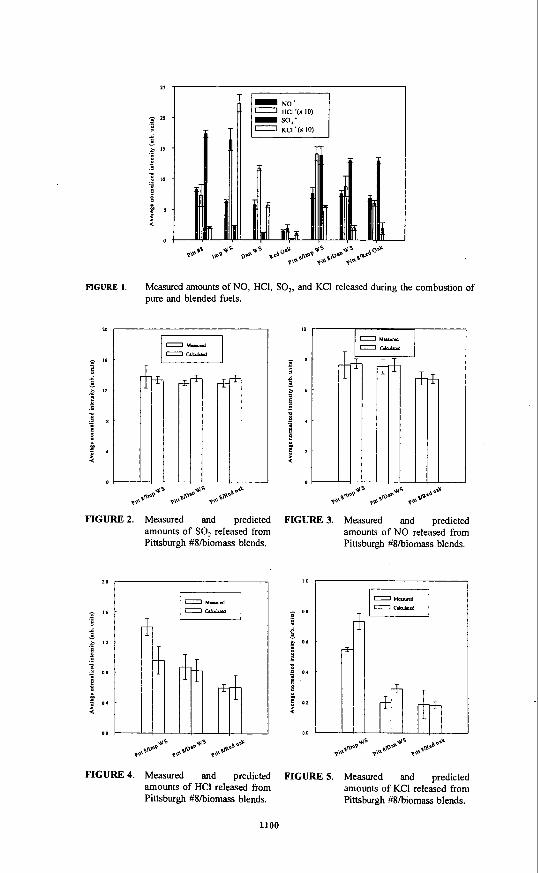
FIGURE 1. Measured amounts of NO. HCI, SO,, and KCI released during the combustion of pure and blended fuels.

20 .

i FIGURE 2. Measured and predicted

amounts of SO, released from Pittsburgh #Skiomass blends.

I O , I

FIGURE 4. Measured and predicted amounts of HCI released from Pittsburgh #S/biomass blends.

I I

FIGURE 3. Measured and predicted amounts of NO released from Pittsburgh #Skiomass blends.

I

FIGURE 5. Measured and predicted amounts of KCI released from Pittsburgh #8/biomass blends.

1100

ATMOSPHERIC EMISSIONS OF TRACE ELEMENTS AT THREE TYPES OF COALFIRED POWER PLANTS

I. Demir', R.'E. Hughes', J. M. Lytlel, and K. K. Ho2 'Illinois State Geological Survey, Champaign, 1L 61820

2111inois Clean Coal Institute, Carterville, IL 62918

INTRODUCTION AND BACKGROUND A number of elements that occur in coal are of environmental concern-because of their potential toxicity and atmospheric mobility during coal combustion. Sixteen of these elements (AS, Be, Cd, C1, Co, Cr, F, Hg, Mn, Ni, P, Pb, Sb, Se, Th, U) are among the 189 hazardous pohtants (HAPS) mentioned in the 1990 Clean Act Amendments (CAA) [US. Public Law 101-549, 19901. The HAPS provisions of the 1990 C&I presently focuses on municipal incinerators and petrochemical and metal industries; a decision on whether to regulate HAPS emissions from electrical utilities will not be made until the U.S. Environmental Protection Agency (EPA) completes its risk analysis.

Numerous studies on environmental aspects of trace elements in coal were reviewed by Swaine 119901, Clarke and Sloss 119921, Wesnor [1993], and Davidson and Clarke 119961. These reviews indicated a high variability of data on trace element partitioning among various phases of coal combustion residues (fly ash, bottom ash, flue gas). Such high variability results from the variations of types and operational conditions of combustion units, the characteristics of coal, and the modes of occurrence of trace elements in the coal. Difficulties in obtaining representative samples and analytical errors also add to the variability of data on trace element emissions from power plants.

In this study, the atmospheric emissions of 12 elements (As, Co, Cr, F, Hg, Mn, Ni, P, Sb, Se, Th, and U ) of environmental concern from three types of power plants burning Illinois coals were inferred from the analytical data on the feed and combustion residues from the plants.

EXPERIMENTAL Samples and Sample Preparation Samples of feed coals and coal combustion residues were collected from a fluidized bed combustion (FBC) plant, a cyclonc (CYC) plant, and a pulverized coal (PC) plant burning Illinois coals (Table 1). A sample of limestone used in the FBC plant was also collected. To prepare for chemical and mineralogical analysis, representative splits of the coal and coarse-grained coal combustion residues were ground to -60 mesh; representative splits of the fine-grained coal combustion residues were prepared by riffling and splitting.

Chemical and Mineralogical Analysis The samples of coal and coal combustion residues were analyzed for major, minor, and trace elements following the procedures of Demir et al. [1994]. The samples were also analyzed for mineralogical composition using x-ray diffraction (XRD) methods. The XRD analysis procedures were described in Demir et al. [1997].

RESULTS AND DISCUSSION Mass balances, emissions, and relative enrichments in the combustion residues were calculated for the 12 elements using the chemical analysis data (Table 2).

Mass balances and emissions. The mass balance value of an element was calculated by comparing the amount of the element in the feed (coal or, in the case of the FBC unit, coal (75%) + limestone (25%)) with the amount of the same element recovered in the combustion residues. The mass balance calculations took into consideration the mass ratios of fly ash to bottom ash, as well as the measured concentrations of ash and elements in the samples, The fly ash to bottom ash ratios were 80/20 for the FBC plant, 25/75 for the CYC plant, and 75/25 for the PC plant.

The mass balances of the 12 elements were normalized to that of AI to eliminate analytical errors. The reason is that AI is a refractory element with relatively high concentration in coal and expected to be retained almost completely in the combustion ashes; less than 5% of AI is expected to escape the particulate collection systems with ultra fine, air-borne fly ash particles. Mass balances of about 100% for AI for the CYC and PC units (Table 2) indicated that the mass balance calculations performed in this study were reliable. The AI mass balance for the FBC unit (76%) was not as good as the AI mass balance for the CYC and PC units; this can perhaps be attributed to the variability in the characteristics of the feeds used in the FBC plant. Both the limestone and the coal used in the FBC unit are blends of products from many different quarries

1101

and mines in Illinois. Therefore, future studies should collect at least several sets of samples over a period of several months of operation from the FBC plant, and the average mass balance data on these samples should be used to smooth out the variance.

If the amount of an element recovered from the combustion residues accounted for 100% of the amount in the feed, then the emission of the element was assumed to be zero. If the mass balance of an element was less than loo%, then the difference was considered to indicate the percentage of the element emitted into the atmosphere through the gas phase or condensation on the ultra fine, air-borne fly ash particles.

For convenience, the emission values were divided into three categories:

Low: <25% Moderate: 25-50% High: >SO%

Negative emission values resulting from the excess mass balance (101-135%) in some cases (Table 2) probably resulted partly from analytical error and partly from contamination of the combustion residues due to the erosion of hardware in the combustion process. Therefore, the negative emission values were assumed to be in the low emission category.

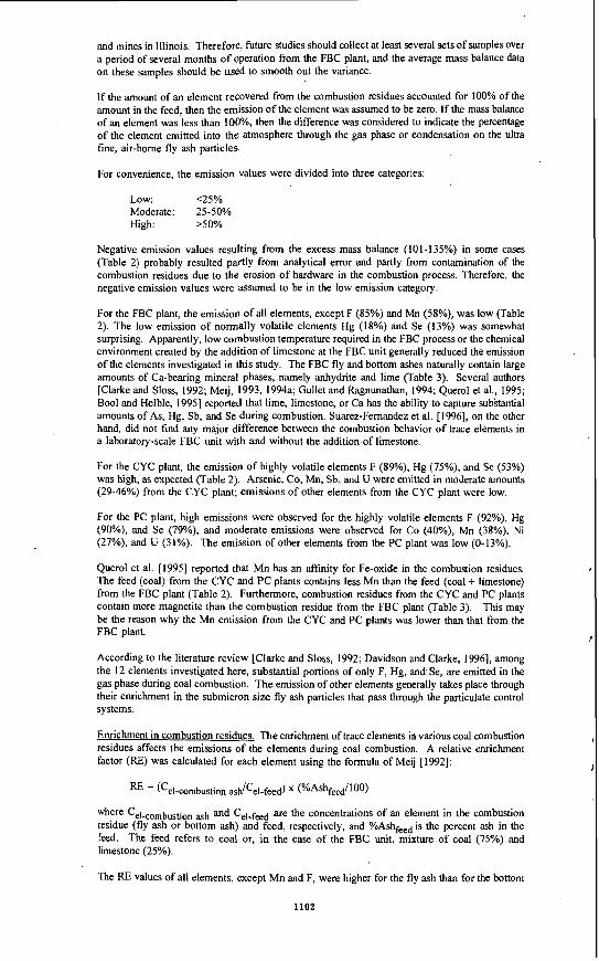
For the FBC plant, the emission of all elements, except F (85%) and Mn (58%), was low (Table 2). The low emission of normally volatile elements Hg (18%) and Se (13%) was somewhat surprising. Apparently, low cornbustion temperature required in the FBC process or the chemical environment created by the addition of limestone at the FBC unit generally reduced the emission of the elements investigated in this study. The FBC fly and bottom ashes naturally contain large amounts of Ca-bearing mineral phases, namely anhydrite and lime (Table 3). Several authors [Clarke and Sloss, 1992; Meij, 1993, 1994a; Gullet and Ragnunathan, 1994; Querol et al., 1995; Boo1 and Helble, 19951 reported that lime, limestone, or Ca has the ability to capture subktantial amounts of As, Hg, Sb, and Se during combustion. Suarez-Femandez et al. [1996], on the other hand, did not find any major difference between the combustion behavior of trace elements in a laboratory-scale FBC unit with and without the addition of limestone.

For the CYC plant, the emission of highly volatile elements F (89%), Hg (75%). and Se (53%) was high, as expected (Table 2). Arsenic, Co, Mn, Sb, and U were emitted in moderate amounts (29-46%) from the CYC plant; emissions of other elements from the CYC plant were low.

For the PC plant, high emissions were observed for the highly volatile elements F (92%), Hg (90%), and Se (79%), and moderate emissions were observed for Co (40%), Mn (38%), Ni (27%), and U (31%). The emission of other elements from the PC plant was low (0-13%).

Querol et al. [I9951 reported that Mn has an affinity for Fe-oxide in the combustion residues. The feed (coal) from the CYC and PC plants contains less Mn than the feed (coal + limestone) from the FBC plant (Table 2). Furthermore, combustion residues from the CYC and PC plants contain more magnetite than the combustion residue from the FBC plant (Table 3). This may be the reason why the Mn emission from the CYC and PC plants was lower than that from the FBC plant.

According to the literature review [Clarke and Sloss, 1992; Davidson and Clarke, 19961, among the 12 elements investigated here, substantial portions of only F, Hg, and Se, are emitted in the gas phase during coal combustion. The emission of other elements generally takes place through their enrichment in the submicron size fly ash particles that pass through the particulate control systems.

Enrichment in combustion residues. The enrichment of trace elements in various coal combustion residues affects the emissions of the elements during coal combustion. A relative enrichment factor (RE) was calculated for each element using the formula of Meij [ 19921:

where Cel-combustion ash and C,I-feed are the concentrations of an element in the combustion residue (fly ash or bottom ash) and feed, respectively, and %Ashfeed is the percent ash in the feed. The feed refers to coal or, in the case of the FBC unit, mixture of coal (750/,) and limestone (25%).

The RE values of all elements, except Mn and F, were higher for the fly ash than for the bottom

1102

\

t

B

ash samples from all three plants (Table 2). The RE value of Mn for the fly ash samples were smaller than or about equal to the value for the bottom ash samples. Fluorine had the Same RE value for both the fly ash and bottom ash samples from the FBC unit. The comparison Of the RE data ofthe elements investigated here indicated that a portion of most of these elements were volatilized during combustion and then upon cooling condensed on the fly ash particles or stayed in the gas phase, or partitioned between the fly ash particles and the gas phase.

Elements that are neither enriched nor depleted in the combustion residue should ideally have RE values of 1. Elements with RE values of greater or less than 1 are enriched or depleted, respectively, in the combustion residue. Based on the literature [Meij, 19921 and for convenience, the RE values in this study were divided into three categories as follows:

NO enrichment or depletion:

Depletion: RE < 0.7

RE = 0.7-1.3 Enrichment: RE > 1.3

The RE values in the combustion products were used in the past to assign the inorganic elements in coal to differing volatility classes [Clarke and Sloss, 1992; Meij, 1992; Davidson and Clarke, 19961. However, such a task is often complicated because of substantial variations in the combustion behavior of elements depending on the characteristics of coal, type and operation conditions of power plants, and the degree of sampling and analytical errors.

Only a few trends common to all three types of plants were apparent from the results of this study (Table 2):

(1) no elements were enriched in the bottom ashes, (2) As, F, Hg, Sb, and Se were depleted in the bottom ashes, and (3) Co, F and Mn were depleted in the fly ashes.

The RE values of other elements varied depending on the ash and plant types investigated. The ' reason why AI, a conservative element, was depleted in the bottom ash of the FBC unit is not

clear although analytical error is a suspect. This study has not examined the enrichment of the trace elements in particle size fractions of the fly ash samples. Previous studies [Meij, 1994b; Tumati and DeVito, 1991, 1993; Dale et al., 1992; DeVito and Jackson, 1994; Helble, 1994; Querol et al., 1995; Cereda et al., 1995; Suarez-Fernandez et al., 19961 indicated that there is generally a positive correlation between ash particle size and the concentration of As, Co, Cr, Hg, Mn, Ni, Sb, and Se.

SUMMARY AND CQNCLUSIONS Mass balances, emissions, and relative enrichment factors (RE) were calculated to determine the combustion behavior of 12 elements (As, Co, Cr, F, Hg, Mn, Ni, P, Sb, Se, Th, U) of environmental concern at three types of power plants burning Illinois coals.

For convenience, the percentage of an element emitted from the power planks was classified as either low (<25%), moderate (25-50%), or high (>50%). Based on this classification, the emission results for the 12 elements were as follows:

low emission moderate emission high emission

FBC plant As, Co, Cr, Hg, Ni, P, Sb, Se, Th, U none F, Mn CYC plant Cr, Ni, P, Th PC plant As, Cr, P, Sb, Th Co, Mn, Ni, U F, Hg, Se

As, Co, Mn, Sb, U F, Hg, Se

Overall low emissions at the FBC plant relative to the other plants likely resulted from either the lower operating temperature compared with other combustion methods or from the creation of a favorable chemical environment as a result of the addition of limestone.

The atmospheric emissions of trace elements are controlled by their volatility and affinity for various coal combustion phases. The elements investigated in this study had higher concentrations in the fly ash than in the bottom ash with a few exceptions. This results from the partial volatilization of the elements from the bottom ash and their subsequent condensation on the fly ash particles upon cooling.

Relative enrichment (RE) values calculated from the composition of feed, fly ash, and bottom ash showed only few trends common to all three plants: (1) no element was enriched in the bottom ashes, (2) As, F, Hg, Sb, and Se were depleted in the bottom ashes, and (3) Co, F and Mn were

1103

depleted in the fly ashes. The RE of other elements varied depending on the ash and plant types.

ACKNOWLEDGEMENTS We thank R. A. Cahill, P. J. DeMaris, Y. Zhang, and J. D. Steele, for analyzing the samples. This study was supported, in part, by grants made possible by the Illinois Department of Commerce and Community Affairs (IDCCA) through the Illinois Coal Development Board (ICDB) and the Illinois Clean Coal Institute (ICCI). Neither the authors, the IDCCA, ICDB, ICCI, nor any person acting on behalf of either: (a) makes any warranty of representation, express or implied, with respect to the accuracy, completeness, or usefulness of the information contained in this paper, or that the use of any information, apparatus, method, or process disclosed in this paper may not infringe privately owned rights; or (b) assumes any liabilities with respect to the use of, or for damages resulting from the use of, any information, apparatus, method, or process disclosed in this paper. Reference herein to any specific commercial product, process or service by trade name, trademark, manufacturer, or otherwise, does not necessarily constitute or imply its endorsement, recommendation, or favoring; nor do the views and opinions of the authors expressed herein necessarily state or reflect those of the IDCCA, ICDB, or ICCI.

REFERENCES Bool, L. E. and Helble, J. J., 1995. A laboratory study of the partitioning of trace elements during

pulverized coal combustion. Energy and Fuels, v. 9, p. 880-887. Cereda, E., Braga, M. G. M., Pedretti, M., Grime, G. W., and Baldacci, A,, 1995. Nuclear

microscopy for the study of coal combustion related phenomena. Nuclear Instruments and Methods in Physics Research, B; B99 (1/4), p. 414-418.

Clarke L. B. and Sloss L. L., 1992. Trace Elements - Emission from Coal Combustion and Gasification. IEA Coal Research, IEACR/49, London.

Dale, L. S., Lawrensic, S. A., and Chapman, J. F., 1992. Mineralogical residence of trace elements in coal - environmental implications of combustion in power plants. CSIRO investigation report CETIIRO58, 79 p.

Davidson, R. M. and Clarke, L. B., 1996. Trace Elements in Coal. IEA Coal Research, IEAPERCII, London.

Demir, I., Harvey R. D., Ruch, R. R., Damberger, H. H., Chaven, C., Steele, J. D., and Frankie, W. T., 1994. Characterization of Available (Marketed) Coals From Illinois Mines. Illinois State Geological Survey, Open File Series 1994-2.

Demir, I., Hughes, R. E., Lytle, J. M., Ruch, R. R., Chou, C.-L., and DeMaris, P. J., 1997. Mineralogical and Chemical Composition of Inorganic Matter from Illinois Coals. Quarterly Technical Report for the period 12/1/1996-2/28/1997 submitted to the Illinois Clean Coal Institute.

DeVito, M. S. and Jackson, B. L., 1994. Trace element partitioning and emissions in coal-fired utility systems. Paper presented at the 87th Annual Mtg. and Exhib. of Air and Waste Management Assoc., Cincinnati, OH, June 19-24, 1994. 94-WP73.03, 16 p.

Gullet, B. K. and Ragnunathan, K., 1994. Reduction of coal-based metal emissions by furnace sorbent injection. Energy and Fuels, v. 8, p. 1068-1076.

Helble, J. J., 1994. Trace element behavior during coal combustion: results of a laboratory study. Fuel Processing Technology, v. 39, p. 159-172.

Mea, R., 1992. A mass balance study of trace elements in a coal-fired power plant with a wet FGD facility. In: Elemental Analysis of Coal and its By-products (ed. G. Vourvopolis). World Scientific Publishing Co., p. 299-3 18.

Meij, R., 1993. The fate of trace elements at coal-fired power plants. Proceedings of 2nd Intern. Conf. on Managing Hazardous Air Pollutants (eds. W. Chow and L. Lewin). EPRl TR-

Meij, R., 1994a. Distribution of trace species in power plant streams: a European perspective. Proceedings of 56th Annual Mtg. of Amer. Power Conf., April 25-27, 1994, Chicago, IL.,

Meij, R., 1994b. Trace element behavior in coal-fired power plants. Fuel Processing Technology,

Querol, X., Femandez-Turiel, J. L., and Lopez-Soler, A,, 1995. Trace elements in coal and their behavior during combustion in a large power station. Fuel, v. 74, p. 331-343.

Suarez-Fernandez, G., Querol, X., Fernandez-Turiel, J. L., Benito-Fuertes, A. B., and Martinez- Tarazona, M. R., 1996. The behavior of elements in fluidized bed combustion. Amer. Chem. SOC. Fuel Chem. Preprints, v. 41. p. 796-800.

104295, p. V83-Vl05, Pal0 Alto, CA.

V. 56-1, p. 458-463.

V. 39, p. 199-217.

Swaine, D. J., 1990. Trace Elements in Coal. Butterworth and Co., London, UK. 276 pp. Tumati, P. R. and DeVito, M. S., 1991. Retention of condensedsolid phase trace elements in an

electrostatic precipitator. In: Managing Hazardous Air Pollutants: State of The Art. EPRI, Palo Alto, CA. 20 p.

Tumati, P. R. and DeVito, M. S., 1993. Trace element emissions from coal combustion - a comparison of baghouse and ESP collection efficiency. Proceedings of 3rd Intern. Conf. on

1104

Effects of Coal Quality on Power Plants. April 25-27, 1993, San Diego, CA. EPRl TR-1- 2280, Palo Alto, CA, p. 3-35 - 3-48.

U.S. Public Law 101-549, 1990. Clean Air Act Amendments, Title 3, 104 Stat 2531-2535. Wesnor J. D., 1993. EPRIEPA SO, Conf., collection of papers, Boston, MA.

Table 1. Amounts and description of coal and coal combustion residues from three types (FBC, CYC, PC) of power plants.

plant Sample Amount Sample type type (Ib) Description'

FBC coal 25 <3/8" size coal fly ash 18 Very fine particle size, light gray color bottom ash 24 <1/4" particle size, mostly yellowish and grayish particles, and small number

of black particles. . limestone 25 Crushed and off-white color

CYC coal 9 Crushed coal fly ash 8 Fine particle size, dark gray color bottom ash 12 <3/8" particle size, black color, and high moistwe content because of

quenching in water FC coal 12 Crushed coal .

fly ash 8 Fine particle size, light gray color bottom ash 15 <3/8" particle size, dark gray to black color, and high

moisture content because of quenching in water

* The size ranges are semiquantitative values based on visual examination.

Table 2. Chemical analysis of coal, coal combustion residues, and limestone samples from three types of power plants, and emission and relative enrichment (RE) values of AI and the 12 elements of environmental concern. The concentration values are in m a g unless indicated otherwise. All the values are on a dry basis.

Plant Sample IOO0"C type type ash,% AI,% As Co Cr F Hg Mn Ni P Sb Se Th U

FBC coal 10.73 1.00 1.8 4.6 25 137 0.10 77 18 131 0.4 5.5 1.8 1.9 fly ash 97.40 3.39 6.1 12.3 75 53 0.25 620 66 567 1.3 14.4 5.6 7.1 bottom ash 97.49 1.09 4.0 4.3 35 48 0.01 310 14 480 0.8 < I 1.9 4.0 limestone 59.18 0.63 3.3 3.5 I I 5 <0.01 1394 9.4262 0.2 G . 5 1.0 2.8

%Mass balance 76 81 16 96 15 82 42 108 104 106 87 94 94 %Emission* 24 19 24 4 85 18 58 0 0 0 13 4 6

RE for fly ash 0.9 0.6 0.6 0.8 0.1 0.7 0.3 1.0 0.8 0.8 0.8 0.8 0.8 RE for bottom ash 0.3 0.4 0.2 0.4 0.1 0.0 0.2 0.2 0.7 0.5 0.0 0.3 0.4

CYC coal 10.48 0.80 2.6 4.0 17 63 0.08 77 8 44 0.7 2.7 1.2 2.0 fly ash 87.52 7.02 50.6 24.2 227 230 0.73 310 173 742 13.6 43.3 14.6 21.7 bottom ash 100.4 8.01 1.2 20.2 112 15 0.02 542 70 524 1.1 2.1 11.3 11.1

' /

I1 %Mass balance 102 54 54 85 I I 25 65 123 135 62 47 104 71 %Emission* 0 46 46 I5 89 75 35 0 0 38 53 0 29

REfor fly ash ' 0.9 2.0 0.6 1.4 0.4 1.0 0.4 2.3 1.8 2.0 1.7 1.3 1.1 t\ RE for bottom ash 1.0 0.0 0.5 0.7 0.0 0.0 0.7 0.9 1.2 0.2 0.1 1.0 0.6

1 PC coal 10.66 0.82 2.2 3.5 17 63 0.08 77 I I 44 0.6 2.9 1.4 2.3 fly ash 97.48 8.47 34.0 20.2 175 67 0.10 468 77 524 7.9 7.4 12.6 16.8 boltom ash 99.96 6.91 3.0 22.2 136 5 <0.01 468 85 262 2.2 2.2 10.4 125

r %Mass balance . 105 121 60 99 8 IO 62 73 106 110 21 87 69 %Emission* 0 0 40 I 92 90 38 27 0 0 79 13 31

RE for fly ash 1 . 1 1.6 0.6 1.1 0.1 0.1 0.6 0.7 1.3 1.4 0.3 1.0 0.8 RE for bottom ash 0.9 0.1 0.7 0.9 0.0 0.0 0.6 0.8 0.6 0.4 0.1 0.8 0.6

%Emission = 100-mass balance. Negative trace element emission values resulting from greater than 100% mass balance were assumed to indicate no emissions (see text).

1105

Table 3. Mineralogical composition of coal combustion residues and limestone from the three power plants.

Mineral content (wt%) Plant Sample type type mullite quartz calcite hematite magnetite anhydrite gypsum lime portlandite amorphous

FBC fly ash 0.0 8.4 0.0 3.0 4.1 31 0.0 2.3 11 40 bottom ash 0.0 8.2 1.9 0.0 0.0 29 2.0 40 13 6.1

CYC fly ash 1.9 7.6 0.8 3.0 14 0.0 5.0 0.0 0.0 68 bottom ash 0.0 1.3 0.0 0.0 1.3 0.0 0.5 0.0 0.0 0 97

PC fly ash 5.1 trace 0.0 2.1 15 1.3 0.0 0.0 0.0 71 bottom ash 0.0 1.0 0.4 2.0 16 0.0 0.0 0.0 0.0 81

___________-__ ~ _.____ ~ -__--------------- ____ ~ __-___ _ _ ______________ __--______ FBC limestone 3.4 % illite, 1.5% kaolinite and chlorite, 5.0% quartz, 86% calcite, and 4.0% dolomite.

1106

I1

A PREDICTION OF COAL ASH SLAGGING UNDER THE GASIFICATION CONDITION

FOR PREPRINTS OF THE AMERICAN CHEMICAL SOCIETY DIVISION OF FUEL CHEMISTRY

Hyun-Taek Kim and Han-jin Bae Energy Department, Ajou University

San 5, Wonchun-Dong, Padal-gu, Suwon, 442-749, Korea

Shi-Hyun Lee Korea Institute of Energy Research

71-2, Jang-Dong, Yusong-gu, Daejon, 305-343, Korea

ABSTRACT Several candidate samples for coal gasification are experimented with proximate, ultimate and ash composition analysis and the fusion temperatures of coal ashes are determined with data from analysis. The effect of flux addition is also evaluated to find the optimum quantity for slagging condition, while considering negative effect of CaO addition on gasification reaction. In order to further expand the variety of candidate coals and the performance in an entrained-bed, the effect of ash fusion temperature drop is evaluated when blending coals. The results of the experiment suggested that optimum compositions of CaO flux are IO%, 20% with Alaska and Datong coal, respectively. However, the optimum value of blending ratio is not known when Posco coal is blended with candidate coals.

INTRODUCTION As the need for electric power increases in Korea, large amounts of imported coal will he utilized in the future. One of the candidate technologies for producing electricity from coal in an environmentally sound manner and high efficiency is IGCC (integrated gasification combined cycle). In a slagging-type IGCC processes, ashes in the coal are cohered and formed slag which is discarded through the bottom of the gasifier. Slagging behavior of coal ash can be enhanced by adding a reduction agent such as limestone and dolomite.

The objective of this study is to predict the slagging and fluid behavior of various coal ashes for the optimum slag removal condition slagging-type IGCC power plants from the physical and chemical characteristics of original coals. The effect of flux addition is studied with candidate coal ash samples to evaluate optimum quantity of flux addition considering negative effect of CaO addition in the coal gasification reaction. The change of ash fusion temperature is also studied to find the optimum blending ratio of Posco coal with Datong coal and Alaska coal. The experimental values of ash fusion temperatures are compared with calculated values so that predictional methodology of ash slagging behavior will be verified within our experimental range. Another objective of the study is to prevent clogging of slag at the bottom of the gasifier which occurs due to solidation of melted slag. The result of this study will be used to determine optimum operation conditions of a 3 T/D slagging-type gasifier which is located in Ajou University, Korea.

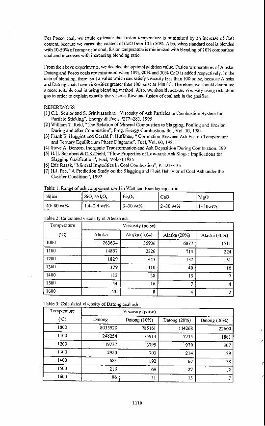
SLAGGING BEHAVIOR IN COAL GASIFIER Slag in the coal gasifier means the melt of coal ash which has constant viscosity and flow along the wall of gasifier. In order to remove ash by the slagging operation, the temperature of the gasifier should be maintained above the fusion temperature of the coal ash. Formed slag should easily flow down to the exit of the gasifier. To maintain this condition, viscosity of the slag should be maintained under the 100 poise [I]. Many empirical equations based on experimental data are proposed in order to explain relationship of chemical composition ofcoal ash and slag viscosity (-51. In the present investigation, Urbain and Watt & Fereday equations are utilized in calculating slag viscosity which give reliable values under 100 poise.

(a) Prediction of slag viscosity Ash slag viscosity can be predicted by Urbain or Watt & Fereday relation. The Urbain equation, in which composition of each slag component is expressed in mole fraction, is derived from CaO-AI,O, S O , three components system. The Urbain equation, as in Eqn (I), is mainly used to determine slag viscosity of low rank coal ash.

1107

In q = In A + In T + 103B/T -A (1)

in equation( I), T is the absolute temperature, A and B are functions of the chemical composition of the ash, and q is the viscosity in poise. Parameter “A’ has different value with the quantity of silica in slag. If the quantity of silica is minimal, slag viscosity can be expanded from Eqns (2)-(13).

A=mT+b

1 O3m=-55.3649F+37.9I 86 b= -I.8244(1O3m)+0.9416

CaO F =

CaO + M g O + N a 2 0 + K 2 0

In A = - (0.2693B+I 1.6725) B= B,+B, (SiO,) + B, @io2)’ +B,(SiO,)’

Bo= 13.8+39.9355a - 4 4 . 0 4 9 ~ ~ ~ B,= 30.481-1 17 .1505~ + 129.9987 a2

B,= - 40.9429 +234.0486a - 300.04 a2 B,= 60.7619-1 53.9276a+211.1616 a2

M e=- M+AI,O,

M = CaO+MgO+Na,O+K,O+Fe0+2Ti0,+3SO, (13)

Meanwhile, in the case of medium silica quantity, Eqn(14)-(16) are used instead of Eqns. (3)-(5)

b= -2.0356(103m)+1 ,1094

F=B(AI,O,+ FeO) - I .3101~+9.9279

When the silica quantity is high in slag, similarly Eqns.(17)-(19) are used instead of Eqns(3)-(5).

b= -1 .7737(103m)+0.0509 103m= -1.7264F+8.4404

SiO,

CaO +MgO +Na,O + K 2 0 (19) F =

Using the Urbain equations in calculating slag viscosity of low rank coal, silica content should be cautiously determined. Silica content mostly affect the B value . In the case of a B value located in the boundary, the larger value is chosen. The experimental result of Watt and Fereday is accepted to determined a reliable relationship between the viscosity of slag and temperature. They proposed Eqn (20), which is derived from regression analysis of experimental data by Hoy et al [6].

1 07m Log,,rl=- +c2 (T - 1 50),

In Eqn. (20), m represents (0.00835 Si02 + 0.00601 AI,O, -1.09) where total percent of (SO, +A1203 +Fe,O,+CaO+MgO) equals 100% and C, is (0.0415Si02+0.0192 AI,O, +0.0276 Fe,O,+ 0.0160CaO-3.92). q is viscosity in poise and T is in OC. This empirical equation is the best fit when the coal ash component is throughly melted so that no crystal exists. Prediction of slag viscosity is correct in the ash component range of Table 1.

The Urbain Watt and Fereday Equation utilized chemical composition of the ash derived by ASTM methods to predict ash fluidity behavior but not the exact behavior of ash fusiodslagging. Calculated viscosity data are represented for Alaska and Datong coal in Table 2 and 3.

(b) Prediction of critical viscosity temperature Liquid phase slag behaves as a Newtonian fluid and, when decreasing temperature, it passes through

1108

.

1

the pseudo-plastic state before solidification. Tlie separation from solid phase depends on the compositioii of slag. When the transition takes place from liquid state to the solid state, the temperature is call Critical Viscosity Temperature (Tcv). Watt [6] derived the equation which is related to chemical composition and Tcv in Eqn(21).

Tcv = 2990-1470(SiO,/AI,O,) + 360(Si02/A1,0,)2-14.7(Fq0,+CaO+Mg0)+ 0.1 5(Fe2O,+CaO+MgO)' (21)

In Eqn (2 I), Tcv is in "C, and the total percent of asli coniponent of SiO, ,AI,O,, Fe,O,, CaO and MgO equals 100. Because of the limitation in using this equation, Tcv can be assigned as a hemispherical temperature determined by tlie ash fusion temperature plus 9 3 T [7].

EXPERIMENT OF ASH SLAGGING CHARACTERISTICS Three different coal samples are utilized for ash fusion teniperature and as11 fluidity behavior. Proximate and ultimate analysis of coal samples are illustrated in Table 4.

From tlie experimental data of ash fusion determination, relationsliip fouling and slagging can be made from the coal combustion and gasification reactions. Determination of not only which coal is tlie best candidate for gasifier or combustor but also whether the dry or wet asli treatment method is appropriate for coal benification. It is well-known that the difference of fusion temperature are related to the degree of fouling and slagging. 'l'he greater the temperature ditlerence between IDT and FT, tlie slower tlie fouling rate so that the intensity of fouling is decrease because more pores are gcnerated in the fouling process.

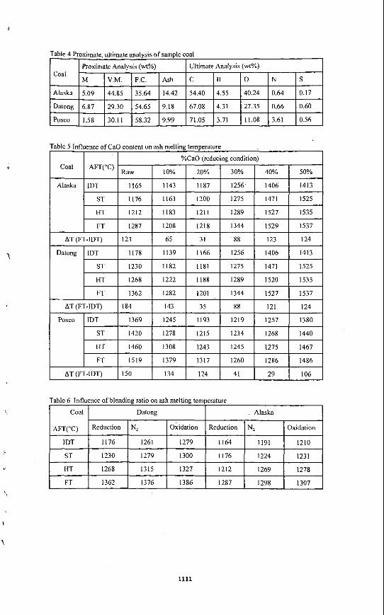
Tlic fusion tcmperaturc of samples has been measured by using the asli fusion deterininator (LECO- 600). Tlie cones were manufacturcd to pyramidal shapc, height I9mm. base 6.5mm. Thc tcmpcraturc of 39OoC, starting temperature of 538"C, final temperature of 1600°C and heating condition and air in oxidizing condition. Table 5 illustrates the nieasuremeiit results of ash temperature of candidate coal while adding CaO as fluxing agent. Ash fusion temperature is decreased with CaO addition until a certain limit but it is increased after that limit because excess addition of CaO results in higher fusion temperature. Table 6 shows the change of tlic asli fusion temperature with mixing ratio and Table 7 shows fusion teniperature change with the coniposition of surrounding gas.

Because ash viscosity measurement is performed in a nitrogen atmosphere, fusion tenipcrature changes with the composition of tlie surrounding gas are evaluated as in Figure 1. Tcv ineasurcd in nitrogen is lower than the Tcv i n air because Fe acted as strong Iluxing agent in the high temperature range. Fusion temperature in a rcducing atmospliere is lower tlian that in the oxidation atmosplicre. The reason is that iron, which plays a significant role i n asli slagging, exists as Fe,O, in an oxidizing environnient but FeO or Fe in reducing one. Actually, the fusion temperature of pure Fe,O, is 1560"C, FeO is 1420°C and Fe is 1275°C. From Table 7, fusion temperature with N, as a surrounding gas is located in the midpoint between those in reduction and oxidation conditions. This result implies that Fe acts as fluxing agent in the inert enviroiiment. AT i n Table 5, wliicli is difference between fluidization temperature and initial dcforiiiation tempcralurc is the index which estimates tlie degree ofslagging. If AT is small, fusion t aka place suddcnly and thin layer of fusion slag is generated. Therefore, to carry out tlie optimal slagging in the gasifier, a candidate coal should be chosen that has an ash composition resulting i n a lower AI' value.

From figure 2 and 3, fusion temperature of Alaska, Datong and Posco coal are mininiuin when IO%, 20% and 30% CaO is added respectively. Also, AT value of Alaska, Datong, Posco coals is niinimuin when 20%, 20%, and 40% CaO is added respectively. Figure 4 shows the rcsults if fusion temperature measurement when mixing Posco coal with Datong and Alaska coals from 10% to 50%, fusion temperatures increased with mixing ratio.

SUMMARY The ob.jectives of this study arc minimi&ition ofthe negative effccts of CaO addition to iiiaiiitaiii a slagging state and expanding the various candidate coals by use of the blending method. We considered the effect of degree of fusion by means of CaO addition and coal blending related with standard coals (Alaska, Datong) and a comparison coal (Posco). First, from the result of fusion temperature measurements when Posco coal with Datong and Alaska coals, fusion temperature is minimum when 10% of CaO is added to Alaska coal, 20% to Datong coal and 50% to Posco coal.

1109

For POSCO coal, we could estimate that fusion temperature is minimized by an increase of CaO content, because we varied the content of CaO from I O to 50%. Also, when standard coal is blended with 10-50% of comparison coal, fusion temperature is minimized with blending of 10% comparison coal and increases with increasing blending ratio.

From the above experiments, we decided the optimal addition value. Fusion temperatures of Alaska, Datong and Posco coals are minimum when IO%, 20% and 30% CaO is added respectively. In the case of blending, there isn’t a value which can satisfy viscosity less than 100 poise, because Alaska and Datong coals have viscosities greater than 100 poise at 1400°C. Therefore, we should determine a more suitable coal in using blcnding mcthod. Also, we should measure viscosity using reduction gas in order to explain exactly the viscous flow and fusion of coal ash in the gasifier.

REFERENCES [ I ] C.L. Senior and S. Srinivasachar, “Viscosity ofAsh Particles in Combustion System for

[2] William T. Reid, “The Relation of Mineral Combustion to Slagging, Fouling and Erosion

[3] Frank E. Huggins and Gerald P. Huffman, “ Correlation Between Ash Fusion Temperature

[4] Steve A. Benson, Inorganic Transformation and Ash Deposition During Combustion, 1991 [5] H.H. Schobert & E.K.Diehl, “Flow Properties of Low-rank Ash Slags : Implications for

[6] Eric Raask, “Mineral Impurities in Coal Combustion”, P. 121-135 [7] H.J. Pac, “A Prediction Study on the Slagging and Fluid Behavior of Coal Ash under the

Particle Sticking”, Energy & Fuel, P277-283, 1995

During and after Combustion”, Prog. Energy Combustion. Sci, Vol IO, 1984

and Ternary Equilibrium Phase Diagrams”, Fuel, Vol. 60, 1981

Slagging Gasification”, Fuel, Vo1.64,1985

Gasifier Condition”. 1997

Silica

40-80 wtyo

SiO, /AI,O, FqO, CaO MgO

1.4-2.4 wt% 3-30 wt% 2-30 wt% 1-30wt%

1110

P

Coal

Alaska

Proximate Analysis (wt%)

M V.M. F.C. Ash C I1 0 N S

5.09 44.85 35.64 14.42 54.40 4.55 40.24 0.64 0.17

Ultimate Analysis (wt%) '

Datong

Posco

6.87 29.30 54.65 9.18 67.08 4.31 27.35 0.66 0.60

1.58 30.11 ' 58.32 9.99 71.05 3.71 11.08 3.61 0.56

Coal

Alaska

%CaO (reducing condition)

AFT("C) Raw 10% 20% 30% 40% 50%

IDT 1165 1143 1187 1256 1406 1413

Datong

ST

HT

1176 1163 1200 1275 1471 1525

1212 1183 1211 1289 1527 1535

1 HT I 1268 I 1222 I 1188 1 1289 I 1520 I 1535 I

FT

AT (FT-IDT)

1287 1208 1218 1344 1529 1537

123 65 31 88 123 124

Posco

IDT 1178 1139 1166 1256 1406 1413

FT

AT (FT-IDT)

AT(FT-IDT) I150 I 134 I 124 1 41 I 29 I 106 I

1362 1282 1201 1344 1527 1537

184 143 35 88 121 124

IDT

ST

IDT I 1176 I 1261 I 1279 I 1164 I 1191 I 1210 I

1369 1245 1193 1219 1257 1380

1420 1278 1215 1234 1268 1440

HT

FT

FT I 1362 I 1376 1 1386 1 1287 I 1298 I 1307 I

1460 1308 1243 1245 1275 1467

1519 1379 1317 1260 1286 1486

1111

Coal

A F T ~ C )

Datong . Alaska

Reduction N, I Oxidation Reduction I N, Oxidation

ST

HT

~~

1230 1279 I300 I I76 I224 1231

1268 1315 1327 1212 1269 1278

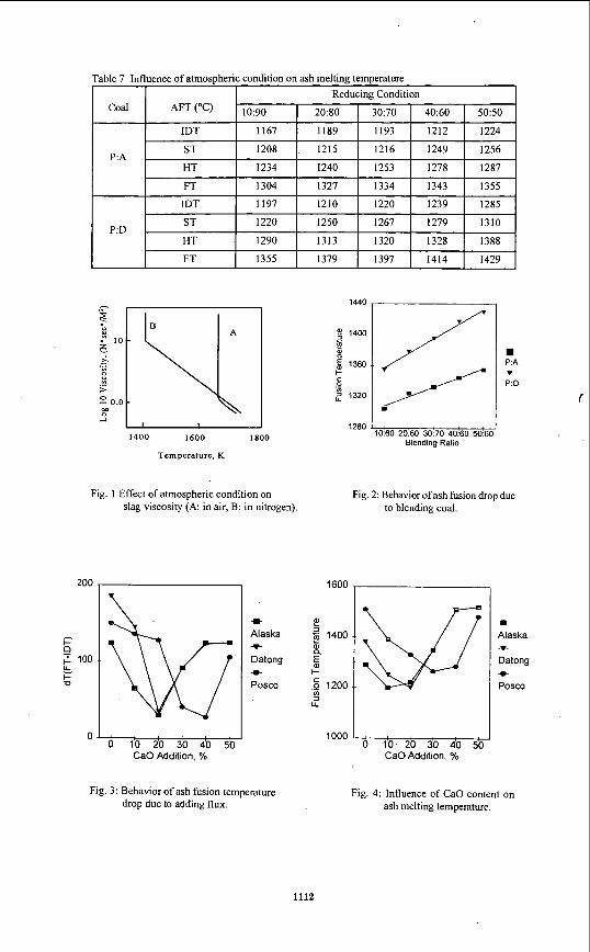
Table 7 Influence of atmospheric condition on ash melting temperature

1400 1600 1800

Temperature, K

Fig. 1 Effect of atmospheric condition on slag viscosity (A: in air, B: in nitrogen).

1360 ! I4O0 1 2 1320

'E I

1440

P:A

P:O v

1280 '1060 2060 30!70 40kO 5060'

Blending Ratio

Fig. 2: Behavior of ash fusion drop due to blending coal.

200

F' Q

o 100 L k

0

b 0 10 20 3b 40 5b

CaO Addition, %

+ Alaska

Datong

Posco

+

*

1600

1400 W a

+ E ._ s 1200 3 LL

1000

Fig. 3: Behavior of ash fusion temperature drop due to adding flux.

- Alaska

Datong

Posco

-t-

+

CaO Addition, %

Fig. 4: Influence of CaO content on ash melting temperature.

1112

1

THE FORMS OF TRACE METALS IN AN ILLINOIS BASIN COAL BY X-RAY ABSORPTION FlNE STRUCTURE SPECTROSCOPY

M.-I.M. Chou, J.A. Bruinius, J.M. Lytle, and R.R. Ruch Illinois State Geological Survey

Champaign, IL 61801

F.E. Huggins and G.P. Huffman University of Kentucky Lexington, KY 40506

K.K. Ho Illinois Clean Coal Institute

Carterville, IL 62918

Abstract Utilities burning Illinois coals currently do not consider trace elements in their flue gas emissions. After the US EPA completes an investigation on trace elements, however, this may change and flue gas emission standards may be established. The mode of occurrence of a trace element may determine its cleanability and flue gas emission potential. X-ray Absorption Fine Structure (XAFS) is a spectroscopic technique that can differentiate the mode of occurrence of an element, even at the low concentrations that trace elements are found in coal. This is principally accomplished by comparing the XAFS spectra of a coal to a database of reference sample spectra. This study evaluated the technique as a potential tool to examine six trace elements in an Illinois #6 coal. For the elements As and Zn, the present database provides a definitive interpretation on their mode of occurrence. For the elements Ti, V, Cr, and Mn the database of XAFS spectra of trace elements in coal was still too limited to allow a definitive interpretation. The data obtained on these elements, however, was sufficient to rule out several of the mineralogical possibilities that have been suggested previously. The results indicate that XAFS is apromising technique for the study of trace elements in coal.

Introduction Currently, Illinois utilities are exempt from having to consider their trace element flue gas emission; however, this may eventually change after the U. S. EPA completes its risk analyses and establishes emission standards. The mode of occurrence of a trace element may determine its cleanability and flue gas emission potential. Trace elements associated with clays and minerals can be reduced by cleaning and those minerals highly dispersed in the coal may be further reduced by advanced cleaning techniques. Also, the volatility of trace elements associated with the organic matrix is different than the volatility of trace elements associated with the inorganic fraction of the coal.

From previous studies of specific gravity testing, many trace elements (such as As, Cd, Mn, Th, and Zn) were shown to have predominantly inorganichineral association’. Some elements (such as Be and B) exhibit an organichaceral association while others (such as Co, Ni, Cu, Cr, and Se) indicate a mixed behavior resulting from different compounds or possibly being highly disseminated in the coal’. Recently, a database of trace element concentrations in a set of 34 commercially utilized coals from the Illinois Basin, which included the Illinois #6 coal used in this investigation, was established2. These data on cleaned and washed samples were compared with those on a set of 222 channel or equivalent samples in the Illinois State Geological Survey records, which represented coal in-place prior to mining and cleaning. A comparison of results indicated that with the exception of uranium (U) and vanadium (V), all other trace elements are reduced in the washed samples as a result of coal cleaning. This phenomenon could suggest that most trace elements may be associated with mineral matter and the U and V in coal may be associated with the organic portion of the coals.

The possibility of misleading results from previous investigations for organichorganic association of trace elements in coal was indicated by many investigators. For example, Finkelman stated that most studies so far offer “little beyond the very rudimentary, and possibly misleading, organichorganic affinity of an element” in coal’. Clarke and Sloss in their review stated that “Genuine organic affinity (organic bonding) has been overestimated in the past, and simple classifications based on rudimentary organic or inorganic affinities may be misleading‘.” It is important to verify previous results with a direct method of determination. This study was conducted to evaluate XAFS techniques as a direct, nondestructive method to determine the mode of occurrence (organichorganic affinity) of trace elements in coal.

1113

Experimental X-ray Absorption Fine Structures (XAFS) spectroscopy, a synchrotron-based technique, is direct and nondestructive. XAFS spectra for Ti and V were obtained at beam-line X19A of the National Synchrotron Light Source (NSLS), Brookhaven National Laboratory, and the XAFS spectra for Cr, Mn, Zn, and As were obtained at beam-line IV3 of the Stanford Synchrotron Radiation Laboratory. Essentially identical experimental procedure was carried out at the two synchrotron facilities. Samples of the coal were exposed to monochromatic X-rays and the fluorescent radiation emitted in response to the X-ray absorption process was detected in a I3 Ge-element solid-state detector. Normally, a scan was made from about 100 eV below the K absorption edge of the element of interest to as much as 1,000 eV above the K-edge. The individual signals recorded in each channel of the 13 Ge-element detector were combined into a single spectral scan. In addition, multiple scans were made for most elements and these scans were also combined to provide a single spectrum for each element. Hence, for most elements, the spectra shown in this paper represent 3 to 5 hours of spectral accumulation time. All spectra were collected and stored on a computer and were transferred electronically to a similar computer at the University of Kentucky for analysis.

The XAFS spectra obtained from different elements in the coal sample were divided into two separate regions: the X-ray Absorption Near-Edge Structure (XANES) region (from -20 to 100 eV of the absorption edge) and the Extended XAFS (EXAFS) region (from 30-50 eV above the edge IO the high-energy limit). The XANES region was used directly as a fingerprint, whereas the EXAFS region was mathematically manipulated further to obtain a radial structure function (RSF) which provided information on the coordination environment of the element. For trace elements, the EXAFS structure is usually only useful if the element is somewhat concentrated (>50 ppm) or if the element is surrounded by heavy elements. Hence, as a consequence of this and other complications, the interpretation of the elemental mode of occurrence was based solely on the XANES region in many cases.

Results Using the data previously obtained on average concentrations of trace elements in coal, a representative Illinois #6 coal sample was chosen for this study2. XAFSKANES spectra were interpreted by comparing them to the spectra of standard compounds. Also, Ti and Mn XAFS spectra of an Argonne #3 coal sample (an lllinois #6 coal from the Argonne Premium Coal Sample) and the Zn XAFS spectra of coals previously studied' were compared with those in this study. The data obtained for the six trace elements in the coal are described as follows:

Arsenic: The Illinois #6 coal as well as its extensively oxidized sample was examined (Figure I) . In both spectra, two distinct peaks were observed, indicating two different forms of arsenic present in these samples. The peak to the negative side of 0 eV arose from arsenic in pyrite (FeAsS), while the higher energy peak arose from an arsenate (AsO,l-) phase, formed by oxidation of the arsenic in pyrite6,'. These assignments were confirmed by examining the RSF derived from the EXAFS region. Although the noise level was high for the arsenic XAFS spectrum of this sample, the RSFs for the two spectra did correctly locate the major peak for the dominant forms at about 2.05 A for arsenic in pyrite and at about 1.30 A for the arsenate anion (Figure 2).

zinc: The spectrum for zinc in the Illinois #6 coal (Figure 3) was strong and was clearly derived largely from zinc sulfide (ZnS). The spectrum was consistent with that seen for other coals from the same seam'. The RSF derived from the EXAFS region for Zn was examined and found to be very similar to that from a ZnS standard (not shown).

Titanium: The titanium spectrum had a relatively weak pre-edge peak at about 3 eV and a broad main peak between 20 and 30 eV that consists of two components (Figure 4).The form of Ti cannot be identified. The spectrum was very similar to that from Ti in Argonne #3 that was examined previouslys. Also, because no sharp minor features were discemable in the spectrum, and because the small pre-edge peak did not exhibit any apparent splitting, virtually all common minerals (rutile, anatase, sphene, Ti-illite, etc.) can be eliminated as being a major contributor to this spectrum.

Vanadium: The University of Kentucky has no database to draw upon to interpret V XAFSKANES spectrum obtained; however, a V rich Kentucky #9 was extensively studied by Maylotte et a18,99. The spectrum of Illinois coal (Figure 5) had a sharp pre-edge feature at about 4 eV which was indicative of either a highly distorted VI' environment or an unusual V" compound This was followed by a two broad peaks from IO to 30 eV. The spectra of the Illinois #6 coal was similar to the spectra of the float fraction of a Kentucky # 9 coal reported by Maylotte et aP9.

1114

'..

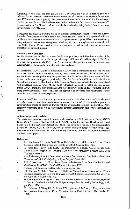
C h m i u m : A very weak pre-edge peak at about 2 eV above the K-edge calibration zero-point indicates that all (>95%) of the chromium was present as C P ; there was no evidence for the more toxic (216' oxidation state (Figure 6). The detection limit was about 5% for CP' for this technique. The Cr spectrum for the Illinois #6 coal was similar to those for Cr in most bituminous coals6.'. Such a spectrum of the Illinois coal was tentatively identified as being derived from a chromium oxyhydroxide (CrOOH) phase.

ManPanese: The spectrum from the Illinois #6 coal used in this study (Figure 7) was quite different from that from Argonne #3' and, except for a weak feature at about 17 eV, appeared to have a profile that was more similar to that of Mn in a lignite (Beulah lignite, ND)'. Additional study using a simulated sample which composited of calcite, illite, and carboxyl material was conducted. The results (Figure 7) suggested its mineral association of calcite and illite and its organic association of carboxyl material.

Summary and Conclusions For the elements As and Zn, the present XAFS data provided a definitive interpretation of the predominant mode of occurrence in the specific sample of Illinois #6 coal investigated. The Zn in this coal was predominately ZnS. The As occurs as either pyritic arsenic or arsenate, and predominately in the arsenate form after extensive oxidation.

For the elements Ti, V, Cr, and Mn; the database of XAFS spectra oftrace elements in coal was still too limited to allow definitive interpretations; however, the data obtained on some ofthese elements were sufficient to make preliminary interpretations. For Ti, the XANES spectrum was sufficient to rule out the minerals suggested previously". The fact that the V XAFS spectra for the Illinois #6 coal was similar to the float fraction of the Kentucky #9 coal may indicate that V was associated with the organic fraction of coal. Most of the Cr in this coal was tentatively identified from coming from a CrOOH phase, but more importantly, the more toxic CP' oxidation state was ruled out from being present in this coal (<5%). The Mn in coal appears to be associated with both mineral (calcite and illite) and organic (carboxyl) phases.

In general, XAFS is a promising technique to determine the mode of occurrence of trace elements in coals. However, more investigations on various coals and standard compounds to produce a larger database should be helpful in drawing solid conclusions for spectrum interpretation. Also, greater understanding of the modes of occurrence of trace elements may help control there flue gas crnission.

Acknowledgment & disclaimer This study was supported, in part, by grants made possible by U.S. department of Energy (DOE) Cooperative Agreement Number DEFC22-PC92521 and the Illinois Coal Development Board (ICDB) and the Illinois Clean Coal Institute (ICCI). Neither authors nor any of the subcontractors nor the U.S. DOE, ISGS, ICDB, ICCI, nor any person acting on behalf of either assumes any liabilities with respect to the use of, or for damages resulting from the use of, any information disclosed in this paper.

References 1.

2.

3.

4.

5. 6.

7.

8.

H.J. Gluskoter, R.R. Ruch, W.G. Miller, R.A. Cahill, G.B. Miller, and J.K. Kuhn, Trace Elements in Coal: Occurrence and Distribution, ISGS Circular 499, 1977. I . Demir, R.D. Harvey, R.R. Ruch, H.H. Damberger, C. Chaven, J.D. Steele, and W.T. Frankie, Characterization of Available (Marketed) Coals form Illinois Mines, ISGS Open File Series 1994-2. R.B. Finkelman, What We Don't Know About the Occurrence and Distribution of the Trace Elements in Coal, J. Coal Quality, v. 8, no. 3-4, pp. 63-66, 1992. L.B. Clarke, and L.L. Sloss, Trace Elements-Emissions form Coal Combustion and Gasification, IEACW49, IEA Coal Research, London, 1992. University of Kentucky XAFS database, unpublished data. F.E. Huggins, N. Shah, J. Zhao, and G.P. Huffman, Nondestructive Determination of Trace Elements Speciation in Coal and Coal Ash by XAFS Spectroscopy, Energy & Fuels, v. 7, no. 4, pp. 482-489, Jul-Aug 1993. G.P. Huffman, F.E. Huggins, N. Shah, and J. Zhao, Speciation of Arsenic and Chromium in Coal and Combustion Ash by XAFS Spectroscopy, Fuel Processing Technology, v. 39, pp. 47-62, 1994. D.H. Maylotte, J. Wong, R.L. St. Peters, F.W. Lytle, and R.B. Greegor, X-ray Absorption Spectroscopic Investigation ofTrace Vanadium Sites in Coal, Science, v. 214, October 30, 1981.

1115

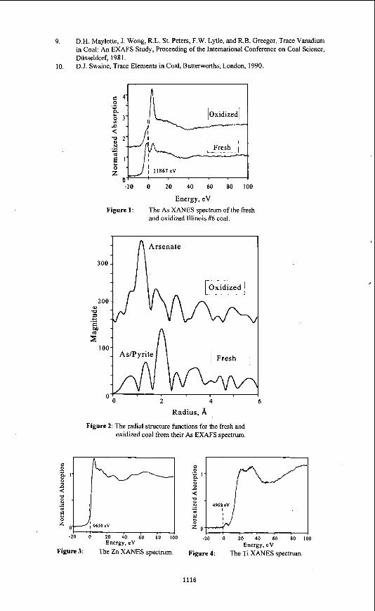
9. D.H. Maylotte, J. Wong, R.L. St. Peters, F.W. Lytle, and R.B. Greegor, Trace Vanadium in Coal: An EXAFS Study, Proceeding of the International Conference on Coal Science, Diisseldorf, 198 1. D.J. Swaine, Trace Elements in Coal, Butterworths, London, 1990. IO.

-20 0 20 40 60 80 100

Energy, eV Figure 1: The As XANES spectrum of the fresh

and oxidized Illinois #6 coal.

" 0 2 4 6

Radius, 8,

Figure 2: The radial structure functions for the fresh and oxidized coal from their As EXAFS spectrum.

9

: U

N ... - z

I 9659sV

-20 0 20 40 60 80 100 Energy, e V

Figure 3: The Zn XANES spectrum. Energy, eV

Figure 4: The Ti XANES spectrum.

1116

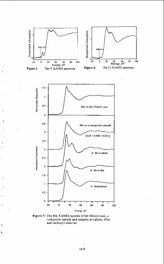
b; 14q5 c v

-20 0 20 40 60 80 100 Energy, e V

Figure 5: The V XANES spectrum

1.5

1

0.5

0

4.5

4

3.5

3

2.5

2

1.5

1

0.5

0

-20 0 20 40 60 80 100 Energy, e V

The Cr XANES spectrum. Figure 6:

Mn in the Illinois coal I

Mn in a composite sample

(0 2A + 0.4% + 0.35 C)

C: Mnkarboxyl

-20 0 20 40 60 BO 100

Energy. eV

Figure 7: The Mn XANES spectra of the Illinois coal, a composite sample and samples of calcite, illite and carboxyl material.

1117

XAFS EXAMINATION OF MERCURY CAPTURE ON THREE ACTIVATED CARBONS

Frank E. Huggins’, Gerald P. Huffman’, Grant E. Dunhain’, and Coiistancc L. Senior’

‘CMWCFFLS, University of Kentucky, Lexington, KY 40506-0043 2University of North Dakola - BBRC, Grand Forks, ND 58202

’Pliysical Scicnces, Inc., Andover, MA 01 810

INTRODUCf ION Mercury is listed as one or the eleven so-called “air-loxics” elements in tlie Amendments to tlie 1990 Clean Air Act [I]. Furthermore, as a result of research stimulated by the passage of this legislation, mercury is now regarded as the single trace elenicnt of greatest concern to utilities generating electrical power from coal combustion, despite its extremely low average concentration in most U.S. coals, typically 0.05 - 0.2 ppm [2,3]. The reasons for this concerti include the volatility of mercury and its compounds, tlie toxicity of its compounds, the ease with which mercury can enter the food chain, particularly by accumulation in fish [4], and tlie huge volunies of coal consumed by tlie power generation industry, wliicli is now approaching one billion tonslyear in the U.S. [ 5 ] .

One promising approach to reducing the atmospheric emission of niercury from coal combustion is the development of sorbent materials tliat cfficiently capture mercury from combustion flue gases at relatively low temperatures (bclow 150°C). Of the many types of inaterials considcrcd for sucli applications, activated carbons have been shown to be among the best. In this work, X-ray absorption fine structure (XAFS) spectroscopy has been employed to examine the mcchanism of mercury capture oii three different activated carbon sorbents. The element-spcci fic nature of the XAFS teclinique has also enabled complementary information to be obtained on the behavior of other important elements present cithcr in the flue gases or in the original carhons.

EXPERIMENTAL (i) Mercury Sorption Experiments Three diffcrcnt activated carbons wcre preparcd at tlic Univcrsity of North Dakota Bncrgy and Environmental Research Center (EERC): a lignite-derived activated carbon (LAC), an iodine- activated carbon (IAC), and a sulfur-activated carbon (SAC). Aliquots or each of tliesc carbons wcrc used i n various experiments at EERC to absorb niercury from a siinulalcd combustion flue gas in a bench-scale reactor. In a typical experiment, about 400 mg of sorbent was held in the simulated flue gas at a tenipcraturc between 225 F and 325 F for a period of up to 16 hours. The baseline flue gas consisted of a synthetic mixture of 6% 0,, 12% CO,, 1600 ppm SO,, 50 ppm HCI, 8% H,O, and the balance N,. Elemenla1 nicrcury was added to the baseline flue gas at a concentration of 60 pg/ni’, altliougli some experiments were run with addition of HgCI, at I2 pg/m’. Three different sets of experiments wcre performed: tlic first set consisted of a comparison of the three sorbents before and aner exposure to tlic simulated flue gas; the second set consisted of the three sorbents exposed to a simulated flue gas containing mercuric chloride (HgCI,); and tlic third set consisted of tlic LAC sorhctil exposed to dirfercnt liorniulalions of the flue gas under otherwise idcnticnl conditioils. Dctails spccific cxpcrilncnts arc sununarizcd in Table I .

(ii) XAFS Experiments The form of mercury and otlier elenients present in tlie activated carbons before and aner the sorption experiments were investigated using XAFS spectroscopy performed at either the Stanford Synchrotron Radiation Laboratory (SSRL), Palo Alto, CA, or tlie National Synchrotron Light Source (NSLS), Brookhaven National Laboratory, NY. At both synchrotrons, a 13-clement gernianium detector [6,7], gated electronically to record the L-edge fluorescence from mercury, was used lo record the niercury L,,, XAFS spectra. A 611 gallium filler was also employed lo inaxiniize the signalhoisc ratio. The XAFS spectra of other elenienls (S, CI, Ca, 1) were recorded at NSLS using a conventional Lytle fluorescence detector [8]. Zero-points of energy for the XAFS spectra of the difrcrent elements are defined as follows: sulfur K-edge - white line peak in elemental sulfur at 2,472 eV; chlorine K-edge - major derivative peak in NaCl at 2,825 eV; calciuni K-edge - major derivative peak in CaCO, at 4,038 eV; iodine L,,, edge - major derivative peak in elemental iodine (I,) at 4,557 eV; and mercury L,,, edge - major derivative pcnk i n clcnicntal mercury at 12,284 cV. Data reduction followed well established proccdurcs [Y.IO]: first, the XAFS spcclrurn was divided into X-ray absorption near-edge struclurc (XANES) and extended X-ray absorption fine structure (EXAFS) spectral regions and each of tliesc regions

/

7

1118

,

1

L

L

was then examined separately. Whereas the XANES spectrum was used without further modification to identify elemental occurrences, the EXAFS spectnun was used to develop a "radial structure function" (RSF). The step-height, determined from the XAFS spectrum as the difference in background absorption above and below the edge, was used as a semi-quantitative measure of the relative concentration of the elements in different sets of samples (Table 2).

TABLE I

Experimental Details for Sorption Experiments

Sample

Filter Temp. H g deg. F Species

Flue Sorbent Gas Hg Mass Conc. mg vdm'

IAC-I IAC-2 LAC- I LAC-2 LAC-3 SAC-I SAC-2

300 60

400 60 500 60

300 60

___

___ __.

Gas Flow Rate m'hr

0.85

0.85 0.85

0.85 -

Length Test

hr Comments

3.37

NA NA

12.42

-- Unreacted

-- Unreacted

- Unreacted

IAC -400 225 HgCI, 400 I2 0.85 12.17 LAC -400 225 HgCI, 400 12 0.85 16.15 SAC -400 225 HgCI, 400 I2 0.85 7.2

LAC-5 225 Hg 400 60 0.85 4.0 IO%O,, bal. N, LAC-6 225 Hg 400 60 0.85 4.0 8%H,O, 10%0,, N, LAC-7 225 Hg 400 60 0.85 4.0 Baseline minus SO, LAC4 225 Hg 400 60 0.85 4.0 Baseline minus HCI

TABLE 2

Relative Step-Heights Determined from XAFS Spectra

Sample S CI Ca I Hg

IAC-I 20 0.1 IAC-2 I I LAC- 1 15 60 6.5 0 LAC-2 18 42 6.0 0 . LAC-3 7 1 0 SAC- I 60 0.9 0 SAC-2 65 I 0

IAC (-400) LAC (-400) SAC (-400)

LAC-5 LAC-6

LAC-8 LAC-I

1 0

2.1 1.5 0

2.8 0

1.5 1.7

1

1.6 1

2.0 6.1

"

" 0 indicates no significant edge detected for that element.

RESULTS AND DISCUSSION (a) Sulfur Sulfur XAFS experiments were carried out on the first suite of seven activated carbons (Table 2). Except for sample IAC-2, the sulfur XAFS spectra were quite strong and different forms of sulfur were readily apparent in the XANES spectra of different samples (Figure 1). Whereas the two SAC samples contained predominantly elemental sulfur (indicated by the major peak at 0 eV), the other samples (IAC-1, LAC) were predominantly sulfate sulfur (indicated by the major peak at IO eV). The LAC samples also contained a minor amount (<lo%) of elemental sulfur. The increase in step-height noted between IAC-1 and IAC-2 and between LAC-I, LAC-2 and LAC-3 suggests that the IAC and LAC carbons may absorb or react with SO,, forming a sulfate species, during exposure to the flue gas. For the two SAC samples, however, there is little

1119

" (blank) field indicates no determination made.

change in sulfur concentration and, moreover, the sulfur form is elemental, which is not consistent with the sulfur speciation in the flue gas as SO,.

(b) Chlorine Chlorine XAFS experiments have been performed only on the three LAC samples in set 1. For the two samples (LAC-I, LAC-2) exposed to the flue gas, a significant increase (approx. 50 times) in chlorine concentration was indicated by the step-height data (Table 2). These data indicate that the LAC carbon readily absorbs chlorine. The chlorine XANES spectra are shown in Figure 2 and are consistent with the capture of chlorine as HCI and not as CI, [ I 11.

(c) Iodine Iodine XAFS experiments were performed on all seven samples in set 1, but as expected, only the two IAC samples gave positive indications of iodine. The iodine L,,, spectra are shown in Figure 3 and appear closest to elemental iodine, although the match is not exact. Whether this reflects a highly dispersed state for elemental iodine in the activated carbons remains to be demonstrated. The step-height data (Table 2) suggest that the iodine content of the carbon after exposure to the flue gas is much less than that before, which may indicate that significant volatilization of iodine from the carbon has occurred during exposure to the flue gas.

(d) Calcium Calcium XAFS experiments were performed only on the two SAC samples and on the two LAC samples exposed to the flue gas. The step-height data for calcium (Table 2) indicate little or no difference in concentration for calcium between the two samples in each pair, suggesting that there is no net loss or gain of calcium during the exposure to the flue gas. The spectra (Figure 4) are distinct for each pair of samples. For the LAC samples, the calcium XANES spectra are similar to that from calcium sulfate (CaSO,) [12]; however, the Ca form that gives rise to the spectra for the SAC samples is not so readily identified.

(e) Mercury The mercury XANES spectra for the four carbon samples in the first sample set that were exposed to the simulated flue gas are shown in Figure 5 . As with all mercury XANES spectra, the fine structure is rather subtle and the first derivative spectrum has been used to accentuate differences among the spectra. As can be seen from the figure, the fine structure becomes more prominent in the order IAC-I < LAC-I, LAC-2 < SAC-I and is accompanied by an increasing separation of the two peaks in the first differential spectra. Based on work on other mercury standards [13], it would appear that the separation of the peaks is highest for ionic mercury compounds and least for covalent and metallic mercury compounds. The observed trend for the peak separation in the activated carbons would be consistent with Hg-S or Hg-CI bonding in the LAC-I, LAC-2 and SAC-I carbons and Hg-I bonding in the IAC-I carbon. Further evidence for this trend can be seen from an analysis of the EXAFS regions of the XAFS spectra presented in Figure 6. The radial structure functions (RSFs) shown in Figure 6 indicate a significantly different local structure for Hg in the iodine-impregnated carbon. In particular, the Hg-X bond for IAC-1 is much longer than those indicated for Hg in SAC-I and for LAC-1,2. The peak positions in the RSFs are consistent with Hg2'-CI, as in HgCI,, andor Hg2+-S, as in HgS (cinnabar), for the LAC-1,2 and SAC-1 samples, and with Hg'+-I, as in HgI,, for the IAC-1 sample. The Hg-S bond distance in HgS (cinnabar) is about 2.36 A, the Hg-Cl-bond distance in HgCI, is about 2.25 A, and the bond distance for Hg-I in HgI, is about 2.78 A.

Very similar mercury XANES spectra to those shown in Figure 5 were obtained from the second set of three samples (IAC -400, SAC -400, LAC -400) that were exposed to the flue gas containing HgCI,. The close similarity of these spectra to those obtained from the corresponding samples exposed to the flue gas containing Hg vapor implies either that the mercury species in the flue gas is the same regardless of whether mercury or mercuric chloride is added to the flue gas, or that the products of the chemisorption reaction on the carbons are not determined by the speciation of mercury in the gas phase, but, rather, are determined by the active species on the carbons. It is also interesting to note that the step-heights derived from the XAFS spectra appear to correlate reasonably well with the durations of the experiments.

Except for differences in the mercury step-height (Table 2) or, equivalently, in the concentration of the mercury captured on the carbons, the spectral data for the LAC samples exposed to different formulations of the flue gas were closely similar to those of other LAC samples investigated previously. Since the experimental conditions were identical, except for the composition of the flue gas, the differences in the mercury step-height must reflect the relative eficiency with which mercuy is captured from the gas stream. It would appear that moisture retards the absorption of mercury, but that HCI and especially SO, enhance the adsorption of elemental mercury. Further experiments will be carried out to confirm these observations.

1120

CONCLUSIONS This work demonstrates that XAFS spectroscopy is a powerful technique for identifying ekmental species on activated carbons and for examining reactions involved in the adsorption of mercury from flue gases on such carbons. Although more work is needed to complete this investigation, a number of interesting conclusions appear to have been reached: ( I ) the mechanism involved in adsorption of mercury appears to depend on the element or method used to activate the carbon; (2) the LAC carbons are very efficient in extracting HCI from the flue gas and both the IAC and LAC carbons appear to react with SO, to form sulfate species; and (3) the adsorption of these gases by the carbons may also aid the adsorption of mercury as the rate of adsorption of mercury appears to be significantly affected by the composition of the flue gas.

'

ACKNOWLEDGEMENTS This work was supported by the U.S. Department of Energy through separate contracts to UND- EERC for preparation of the activated carbons and to PSI and UK for research on the "air-toxics" elements. Both contracts were also supplemented by the Electric Power Research Institute. We also wish to acknowledge Tom Brown, U.S. DOE-FETC, in bringing these efforts together. The U.S. DOE is also acknowledged for its support of the Synchrotron Radiation Laboratories, SSRL and NSLS, without which the XAFS experimentation could not have been carried out.

REFERENCES 1. 2.

3. 4. 5.

6.

7. 8.

9.

10.

11. 12.

13.

US. Public Law 101-549, U.S. Government Printing Offm, Nov. 15th, 1990, 314 pp. Bragg, L.J., Oman, J.K, Tewalt, S., Oman, C.L., Rega, N.H., Washington, P.M. and Finkelman, R.B., Coal quality (COALQUAL) database: version 1.3. U.S. Geological Survey, Open-File Report 94-205, 35Mb CD-ROM, 1994. Swaine, D.J., Trace Elements in Coal, Butterworths, 1990. Porcella, D., EPRI Journal, pp. 46-49, Apr/May 1990. Richardson, C.V., and Nielsen, G.F., (eds.), 1980 Keystone Coal Indushy Manual, McGraw-Hill, New York, NY, 1980. Cramer, S.P., Tench, O., Yocum, N., and George, G.N., Nucl. Instrum. Methods A266, 586-591, 1988. Huggins, F.E., and Huffman, G.P., Intern. J. Coal Geol. a 31-53, 1996. Lytle, F.W., Greegor, R.B., Sandstrom, D.R., Marques, E.C., Wong, J., Spiro, C.L., Huffman, G.P., and Huggins, F.E., Nucl. Instrum. Methods 226, 542-548, 1984. Lee, P.A., Citrin, P.H., Eisenberger, P.A., and Kincaid, B.M., Rev. Mod. Phys. a 769- 808, 1981. Brown, Jr., G.E., Calas, G., Waychunas, G.A., and Petiau, J., Chapter 11 in: Reviews in Mineralogy, Vol. 18, Mineral. SOC. America, Washington DC, pp. 431-512, 1988. Huggins, F.E., and Huffman, G.P., Fuel a 556-569,' 1995. Huffman, G.P., Huggins, F.E., Levasseur, A.A., Durant, J.F., Lytle, F.W., Greegor, R.B., and Mehta, A,, Fuel, a 238-242, 1989. Huggins, F.E., et al., unpublished work.

9

8

7

6

5

4

3

2

1

O ' J -10 10 30

Energy, eV

Figure I : Sulfur XANES of activated carbons.

0.4 . 0.2 ' 0 1 - . . . . . . .

-20 0 20 40 Energy, eV

Figure 2: Chlorine XANES of LAC activated carbons.

1121

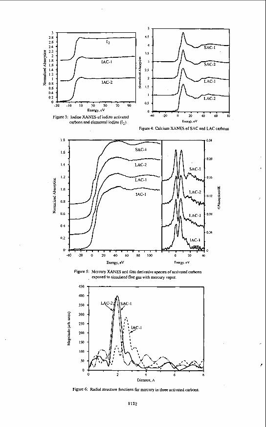
Figure 3: Iodine XANES of iodine activated -40 -20 0 20 40 60 80

carbons and elemental iodine (Iz). E ~ g y . eV

Figure 4: Calcium X A N E S of SAC and LAC carbons.

1.8

1.6

I .4

1.2 0 .- '. f 1.0 d B 2 0.8

I ' 0.6

0.4

0.2

SAC- I

LAC-2

IAC-1

0 -40 -20 0 20 40 60 80 100

Energy, eV

0.20

0.16

0.12

0.08

0.W

0 0 20 40

Energy. eV

Figure 5: Mercury XANES and first derivative spectra of activated carbons , exposed to simulated flue gas with mercury vapor.

400

350

Y 300

$ 250

- 'I v

4 200

$ 150

IO0

50

0 0 ' 2 4 6 8

Distance, A

Figure 6: Radial structure functions for mercury in three activated carbons.

1122

,

, .,

I

STRUCTURAL CHARACTERISTICS AND THERMAL STABILITY OF FGD SCRUBBER SLUDGE

P. S. Valimbe",V. M. Malhotra",and D. D. Banerjeeb a. Department of Physics, Southern Illinois University, Carbondale, IL 62901

b. Illinois Clean Coal Institute, Carterville, IL 62918.

ABSTRACT

We investigated the structural and thermal properties of flue gas desulfurization (FGD) scrubber sludge (CWLP, Springfield, Illinois) to explore this residue's suitability for conversion into structural materials. The structural characteristics of the sludge were obtained by undertaking transmission-Fourier transform infrared (FTIR), diffuse reflectance-FTIR (DRIFT), and scanning electron microscopy (SFM) measurements, while the thermal stability of the residue was gauged by conducting differential scanning calorimetry (DSC) and differential thermal analysis (DTA) experiments at 30°C < T < 1150°C. The SEM data and vibrational results suggest that this fesidue is largely gypsum and contains a few particles of fly ash. We did observe only very weak sO3'- bands in the sludge's FTIR spectrum. The sludge is ,primarily composed of two types of crystallites, i.e., rectangular-shaped needles and parallelogram-shaped crystals. The thermal results on the sludge indicate that the water is lost from the sample in a two step process at 150°C < T < 200°C. The observed dehydration enthalpy of 585 J/g was higher than that reported for gypsum. However, our results are consistent with the commercial gypsum samples we tested. After exothermic transformation at 380°C. the sludge sample and the commercial gypsum samples remained thermally inert at 400°C < T < 1150°C.

INTRODUCTION

Presently more than 90 million tons of coal combustion byproducts, i.e., fly ashes, bottom ashes, and scrubber sludges, are generated in the U.S. annually. These byproducts' yield is expected to grow in the near future as the Clean Air Act is stringently enforced [I-31. The Midwestern USA coals are high in sulfur content, and the combustion of these coals results in emissions containing a high percentage of SO.. Flue gas desulfurization (FGD) technology is commonly used in order to reduce the emission of these venomous gases. Some power plants use a scrubber unit to capture SO,, and this produces about 20 million tons of scrubber sludge in the USA alone.

It is generally believed that the major components of scrubber sludge, depending upon whether it is a forced oxygen unit, are calcium sulfite (CaSO,), calcium sulfate (CaS04), and gypsum (CaS04.2H20). In addition, small amounts of fly ash and excess scrubbing reagents have been reported in the sludges. When lime or limestone is used as a sorbent material in the FGD systems, the purity of calcium sulfate obtained as a byproduct ranges between 95% to 99%. Lime reacts with SO2 in the scrubber unit, and different products are formed depending on the temperature of the system. It has been reported that only CaSO, was formed below 550"C, while a mixture of CaSO,, CaS04 and CaS was produced at 600°C < T < 850°C [4]. Above 800°C, only CaS04 and Cas were formed. On the other hand, if CaCOl is used in a scrubber unit, different byproducts are formed depending on the temperature at which the flue gases react with it. The reactions of CaCO, with air ( 0 2 ) + SO1 have been thoroughly investigated at different temperatures [5]. I t was found that the amount of sulfite formed in such a system was always small compared to the other phases. Significant amounts of CaSO, were formed only at T > 600°C. Formation of Cas04 was extremely low but detectable at temperatures above 400°C. At T h 6OO0C, the formation of CaSO, was significant and reached a maximum at 800°C. Other traces detected above 800°C were CaCO,, CaO, Cas, CaSO,, and Ca(OH)>.

It has been reported that the hydrated calcium sulfate, particularly gypsum, produced as a byproduct of scrubbing flue gases, could be used in a variety of applications. Most of the scrubber sludge produced in the U.S. is currently used only in landfill applications [1-3]. Some other applications of this residue are road construction [6], wallboard manufacturing [7], and agricultural [8]. However, the quantity of these residues produced as well as the cost of disposal are very large and are increasing every year. Hence, it is necessary to develop more applications in which these residues can be utilized. If the gypsum is to be used in different market applications, the fly ash must be removed from the flue gas before the scrubbing process to avoid contamination. Also, it is necessary to ascertain whether scrubber sludges produced are environmentally safe,

1123

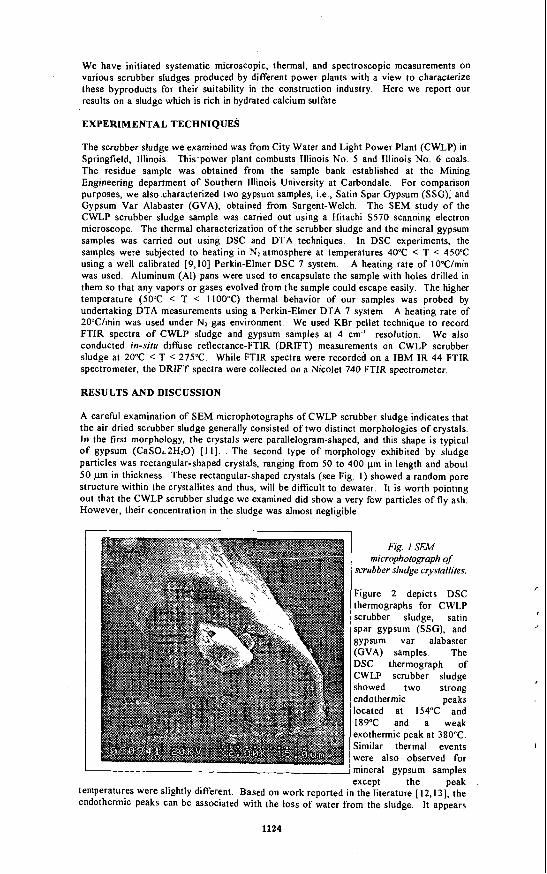
We have initiated systematic microscopic, thermal, and spectroscopic measurements on various scrubber sludges produced by different power plants with a view to characterize these byproducts for their suitability in the construction industry. Here we report our results on a sludge which is rich in hydrated calcium sulfate

EXPERIMENTAL TECHNIQUES

The scrubber sludge we examined was from City Water and Light Power Plant (CWLP) in Springfield, Illinois. This-power plant combusts Illinois No. 5 and Illinois No. 6 coals. The residue sample was obtained from the sample bank established at the Mining Engineering department of Southern Illinois University at Carbondale. For comparison purposes, we also characterized two gypsum samples, i.e., Satin Spar Gypsum (SSG); and Gypsum Var Alabaster (GVA), obtained from Sargent-Welch. The SEM study of the CWLP scrubber sludge sample was carried out using a Hitachi S570 scanning electron microscope. The thermal characterization of the scrubber sludge and the mineral gypsum samples was carried out using DSC and DTA techniques. In DSC experiments, the samples were subjected to heating in N2 atmosphere at temperatures 40°C < T < 450°C using a well calibrated [9,10] Perkin-Elmer DSC 7 system. A heating rate of 10Wmin was used. Aluminum (AI) pans were used to encapsulate the sample with holes drilled in them so that any vapors or gases evolved from the sample could escape easily. The higher temperature (50°C < T < 1100°C) thermal behavior of our samples was probed by undertaking DTA measurements using a Perkin-Elmer DTA 7 system. A heating rate of 20"C/min was used under N1 gas environment. We used KBr pellet technique to record FTIR spectra of CWLP sludge and gypsum samples at 4 cm.' We also conducted in-situ diffuse reflectance-FTIR (DRIFT) measurements on CWLP scrubber sludge at 20°C < T < 275°C. While FTIR spectra were recorded on a IBM IR 44 FTIR spectrometer, the DRIFT spectra were collected on a Nicolet 740 FTIR spectrometer.

RESULTS AND DISCUSSION

resolution.

Fig. I SEA4 microphotograph of

scrubber sludge ctyslalliles.

Figure 2 depicts DSC thermographs for CWLP scrubber sludge, satin spar gypsum (SSG), and gypsum var alabaster (GVA) samples. The DSC thermograph of CWLP scrubber sludge showed two strong endothermic peaks located at 154°C and 189°C and a weak exothermic peak at 380°C. Similar thermal events were also observed for

I mineral gypsum samples

A careful examination of SEM microphotographs of CWLP scrubber sludge indicates that the air dried scrubber sludge generally consisted of two distinct morphologies of crystals. In the first morphology, the crystals were parallelogram-shaped, and this shape is typical o f gypsum (CaSO4,2H2O) [ l l ] . The second type of morphology exhibited by sludge particles was rectangular-shaped crystals, ranging from 50 to 400 pm in length and about 50 pm in thickness. These rectangular-shaped crystals (see Fig. 1) showed a random pore structure within the crystallites and thus, will be difficult to dewater. It is worth pointing out that the CWLP scrubber sludge we examined did show a very few particles of fly ash. However, their concentration in the sludge was almost negligible.

i

i i

that the dehydration reaction in our CWLP scrubber sludge sample occurred in two steps, just as it has been reported for CaSOI.2H20 [13]. The peak at 154°C may be due to the loss of 1.5 water molecules which resulted in the formation of hemihydrate, CaS04.0.5H20. The dehydration further continued when at 189"C, y-anhydrite was formed by the loss of the remaining 0.5 water molecule. Even though there are some dissimilarities in the peak positions of the observed endothermic and exothermic reactions observed for CWLP scrubber sludge and mineral gypsum samples, we believe the CWLP scrubber sludge is largely composed of CaS02.2H20

100 200 300 400 TEMPERATURE ('(2)

Fig. 2 DSC thermographs of (A) CWLP scrubber sludge, (B) Sarin Spar Gypsum (SSG), and (c) Gypsum Var Alabaster (GVA) samples. The two endothermic peaks at 100°C < T

< 200°C represent decomposition and desorpfion of water from the samples.

Our results indicate that the enthalpy of dehydration reaction for CWLP scrubber sludge was 592 J/g, which is much larger than that reported by Strydom et al. [I41 for synthetic gypsum. Strydom et. al., using DSC technique, reported that the dehydration enthalpy of synthetic gypsum varied over a range of 377 J/g t o 420 J/g. However, DSC experiments conducted on mineral gypsum samples in our laboratory revealed a value of 656 J/g and 704 J/g for GVA and SSG, respectively. Since the observed dehydration enthalpy.wil1 be strongly influenced by such factors as packing of the particles in the AI pans, the consistency and uniformity of the holes in the pans, and the ramping rates used, some variation in the enthalpy value is expected. However, to provide conclusive evidence, additional experiments will be needed and are in progress.

Table 1 summarizes our DTA results on scrubber as well as mineral gypsum samples at 50°C < T < 1100°C. Similar to DSC results, the DTA experiments on the sludge exhibited a two-step dehydration reaction. This was followed by a polymorphous transformation, Le., y-CaSOn transforms into 0-CaSO4 at 380°C. After the formation of 0-anhydrite at 380°C. the DTA results did not show any other thermal event either for sludge or mineral gypsum samples at 380°C < T < 1100°C.

We attempted to ascertain the chemical structure and composition of CWLP scrubber sludge by conducting FTIR spectroscopic measurements. The infrared (IR) frequencies along with the observed peak heights are reproduced in Table 2. Also listed in Table 2 are the IR band frequencies for mineral gypsum samples. The IR spectrum of scrubber sludge showed two vibrational modes at 3615 cm' (v, stretch of HO-H)) and 3557 cm-' (vl stretch of HO-H) in the water's stretching region, while a single oscillator at 1620 cm-' was observed in the water's bending region. On the other hand, the mineral gypsum samples showed three vibrational bands in the water's stretching region and two IR bands in the water's bending region. Bensted and Prakash [ 151 have suggested that the different phases of calcium sulfate can be distinguished by the vibrational modes of water observed. For example, 0 - H stretching vibrations are observed at - 3555, - 3500, and - 3400 cm.' in the water's stretching region for gypsum (CaS04.2HzO) along with two oscillators at - 1680 and - 1620 cm.l in the water's bending region. Hemihydrate (CaS04.0.5HzO)

1125

Sample Peak Begins at ("C)

CWLP 93 Scrubber 335 Sludge

Satin Spar 64 Gypsum 330

Gypsum Var 97 Alabaster 338

602 (0.50) I 602 (0.30) I 602 (0.30) I

We performed in-situ DRIFT measurements at 20°C < T < 260°C on air-dried CWLP scrubber sludge to answer whether this sludge was in gypsum or hemihydrate phase. Figure 3 reproduces how temperature altered the DRIFT spectrum of the sludge. At 30°C the sludge's DRIFT spectrum showed four vibrational bands in the water's stretching region, Le., a t 3556, 3489, 3402, and 3249 c m ' and two bands at 1687 and 1620 cm'l in the water's bending region. As the temperature was raised above 30°C. the band at 3556 cm-' lost intensity and shifted to 3570 cm" at 106°C. The band at 1687 cm.' rapidly lost intensity at 106°C and disappeared at 135°C. At 135°C < T < 18OoC, we observed two bands at 3630 and 3550 cm" in the 0-H stretching region and a single band at around 1624 cm.' in the water's bending region. Above T > 180°C, the H-0-H bands were very weak ifthey were observed at all. Based on our in-sifu DRIFT results, we believe CWLP scrubber sludge mostly contains gypsum phase which readily loses water a t 50°C < T <

1126

Peak End at Peak Remark ("C) Temperatures

273 165, 181 Endothermic 480 3 80 Exothermic

316 203 Endothermic 480 3 78 Exothermic

300 183, 193 Endothermic 432 3 79 Exothermic

("C)

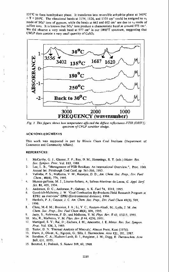
135°C to form hemihydrate phase. It transforms into reversible anhydrite phase at 160°C < T < 260°C. The vibrational bands at 1154, 1126, and 1105 cm-' could be assigned to VI

mode of Sod2. ions of gypsum, while the bands at 662 and 602 cm-' are due to v4 mode of sulfate ions. It is known that SO? ions produce a characteristic band at around 975 cm". We did observe a very weak band at 977 cm-' in our DRIFT spectrum, suggesting that CWLP does contain a very small quantity of CaSO,.

1 I I

3000 2000 1000 FREQUENCY (wavenumber)

Fig. 3 This figure shows how temperature affected the dvfuse rejlectance-FTIR (DlUFT) spectrum of CWLP scrubber sludge.

ACKNOWLEDGMENTS

This work was supported in part by Illinois Clean Coal Institute (Department of Commerce and Community Affairs).

REFERENCES:

1. McCarthy, G. J.; Glasser, F. P.; Roy, D. M.; Hemmings, R. T. (eds.)Mater. Res. SOC. Sympos. Proc. Vol. 113, 1988.

2. Lee, L. B., "Management of FGD Residues: An International Overview.", Proc. 10th Annual Int. Pittsburgh Coal Conf, pp. 561-566, 1993.

3. Valimbe, P. S.; Malhotra, V. M.; Banerjee, D. D.; Am. Chem. SOC. Prep., Div. Fuel Chem., 40(4), 776, 1995.

' 4. Munoz-guillena, M. J., Linares-Solano, A; Salinas-Martinez de Lecea, C. Appl. Surf. Sci. 81, 409, 1994.

5 . Anderson, D. C.; Anderson, P.; Galway, A. K. Fuel 74, 1018, 1995. 6. Goodrich-Mahoney, J. W. "Coal Combustion By-products Field Research Program at

EPRI: an overview" EPRI (Environmental division), 1994. 7. Henkels, P. J.; Gaynor, J. C. Am. Chem. SOC. Prep., Div. Fuel Chem 41(2), 569,

1996. 8. Chou, M.-I. M.; Bruinius, J. A,; Li, Y. C.; Rostam-Abadi, M.; Lytle, J. M. Am.

Chem. SOC. Prep., Div. Fuel Chem 40(4), 896, 1995. 9. Jasty, S.; Robinson, P. D.; and Malhotra, V . M. Phys. Rev. B 43, 13215, 1991. IO . Mu, R.; Malhotra, V. M. Phys. Rev. B 44, 4296, 1991. 11. Mattigod, S. V.; Rai, D.; Zachara, J. M.; Amonette, J. E. Mater. Res. SOC. Sympos.

Proc. Vol. 136, 3 , 1989. 12. Todor, D. N. 'Thermal Analysis ofMinerals', Abacus Press, Kent (1976). 13. Dunn, J.; Oliver, K.; Nguyen, G.; Sills, 1. Thermochim. Acta 121, 181, 1987 14. Strydom, C. A.; Hudson-Lamb, D. I.; Potgieter, J. M.; Dagg, E. Thermochim. Acta

269, 631, 1995. 15. Bensted, J.; Prakash, S. Nature 219, 60, 1968.

1127

the effects of fjel-bound chlorine and alkali on corrosion ... archive/files/merge/vol-42... · the...

Documents