1

Earth and Planetary Science Letters 164 (2004) 1-10

EPSL Frontiers

The evolution of El Niño, past and future

Mark A. Cane

Lamont-Doherty Earth Observatory of Columbia UniversityPalisades, NY 10964-8000

Abstract

We review forecasts of the future of El Niño and the Southern Oscillation (ENSO), a coupledinstability of the ocean-atmosphere system in the tropical Pacific with global impacts. ENSO inthe modern world is briefly described, and the physics of the ENSO cycle is discussed.Particular attention is given to the Bjerknes feedback, the instability mechanism which figuresprominently in ENSO past and future. Our knowledge of ENSO in the paleoclimate record hasexpanded rapidly within the last 5 years. The ENSO cycle is present in all relevant records,going back 130 kyr. It was systematically weaker during the early and middle Holocene, andmodel studies show that this results from reduced amplification of anomalies in the late summerand early fall, a consequence of the altered mean climate in response to boreal summerperihelion. Data from corals shows substantial decadal and longer variations in the strength ofthe ENSO cycle within the past 1000 years; it is suggested that this may be due to solar andvolcanic variations in solar insolation, amplified by the Bjerknes feedback. There is someevidence that this feedback has operated in the 20th century and some model results indicate thatit will hold sway in the greenhouse future, but it is very far from conclusive. Thecomprehensive general circulation models used for future climate projections leave us with anindeterminate picture of ENSO’s future. Some predict more ENSO activity, some less, with thehighly uncertain consensus forecast indicating little change.

1. IntroductionGiven time, we are a very adaptable species. Humans survive, and even flourish, in climatesranging from tropical to arctic, from arid to rain forest. In common with most species, however,we are troubled by rapid changes in climate. A few years of well below average rainfall insome normally well-watered farmlands may fairly be described as “a devastating drought”,although the same level of rainfall might mean a bountiful harvest in a savannah.

Within our lifetimes, the most dramatic, most energetic, and best-defined pattern of climatechanges has been the global set of anomalies referred to as ENSO (El Niño and the SouthernOscillation). The very strong and very heavily reported event in 1997-98 brought El Niñoworldwide notoriety. It is implicated in catastrophic flooding in coastal Peru and Ecuador,drought in the Altiplano of Peru and Bolivia, the Nordeste region of Brazil, and Indonesia, New

2

Guinea and Australia. Huge forest fires on Kalimantan spread a thick cloud of smoke overSoutheast Asia and crippled air travel by shutting down airports in Singapore, Malaysia andIndonesia.

While there is a tendency to hold El Niño responsible for just about anything unusual thathappened anywhere, the listed climate impacts are ones that investigations of events in the pastcentury have shown to be strongly correlated with El Niño. Of course, every year there aredroughts and floods somewhere. Goddard (2004) points out that, paradoxically, El Niño yearsmay come to be the least costly. Unlike the seemingly random set of climate hazards in atypical year, those associated with El Niño are predictable a year or more ahead (Goddard et al2001; Chen et al 2004). This could allow preparations that would mitigate the impacts of ElNiño related climate anomalies. For example, given prior warning of the 1997-98 El Niño, inanticipation of heavy rains the city of Los Angeles cleared storm drains to prevent flooding.Even without good predictions of particular events, there can be adaptive advantages just inknowing the longer-term patterns. Farmers in Queensland now understand that as aconsequence of the ENSO cycle, it is likely that they will make money only 3 years out of 10,and plan accordingly. In Guns, Germs and Steel, Jared Diamond argues that since agriculturewas doomed to fail so often, aboriginal Australians were correct to remain as hunter-gatherers, achoice with the most profound cultural consequences.

All of us now anticipate a change in climate brought about by human activity. Among otherthings, we will have to adjust to a change in the year-to-year variations in climate. Will there bemore El Niños, or more powerful El Niños? Will the impacts of the ENSO cycle change? Overthe past century, the period for which we have instrumental data, there is a statisticallysignificant association between poor monsoons in India and El Niño events. This relationshipseemingly broke down in the 1990s (Kumar et al, 1999); monsoon rainfall was near normalduring the powerful 1997 event. In contrast during the very strong 1877 El Niño there wassevere drought in Indian leading to widespread famine. Kumar et al (1999) speculated that thechange in the monsoon-ENSO relationship might be a consequence of global warming.However, the “normal” association seemingly has returned, as the moderate 2001-02 El Niñowas accompanied by a weak monsoon.

So, how will El Niño change in a greenhouse world? The short answer, to be expanded upon inSec. 4, is that the best estimate is that it will not change much at all, but we have very lowconfidence in this answer. We begin in Sec 2 with a brief review of salient features of ENSOobserved in the modern, instrumental record. We touch on ideas about the physics of ENSO,ideas that are useful in considering how ENSO behavior can change. ENSO’s past is reviewedin Sec. 3. The last few years have seen a great increase in our knowledge of ENSO in theHolocene and late Pleistocene. The changes over this time, and our ability to explain them,offer some guidance for the future.

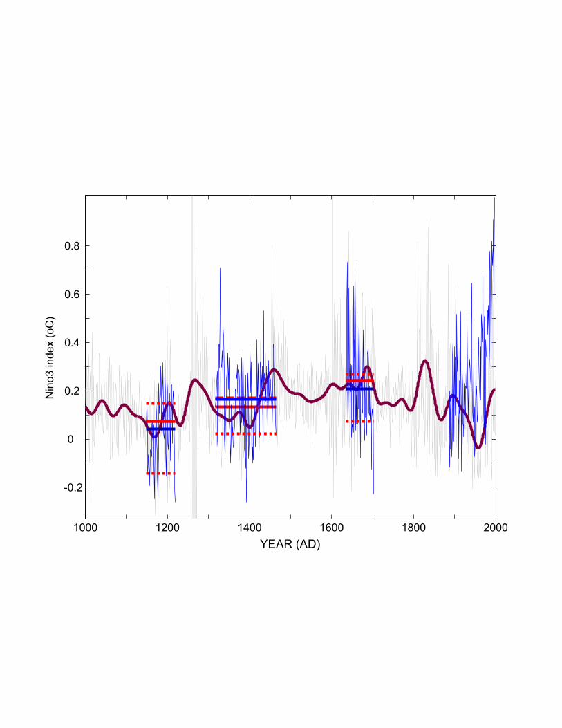
2. ENSO in the PresentFigure 1 shows two widely used indices for ENSO over the past century and a half. The term“El Niño” was used long ago by Peruvian fisherman for the annual warming of coastal watersthat occurs around Christmas time. Scientists now reserve the term for a warming of the easternequatorial Pacific, though there is no widely accepted definition of how much of a warming

3

over exactly what region it takes to qualify as an “El Niño”. NINO3, which refers to the seasurface temperature (SST) anomaly in the NINO3 region (90W-150W, 5S-5N) of the easternequatorial Pacific, is a commonly used index of El Niño. The “Southern Oscillation” is a see-sawing of atmospheric mass, and hence of sea level pressure (SLP), between the eastern andwestern Pacific. It is most often indexed by the Southern Oscillation Index (SOI), a normalizedSLP difference between Darwin, Australia and Tahiti. In Fig. 1 we simply use SLP at Darwin,which is almost the same because the anti-correlation between Tahiti and Darwin is so high.There is a striking similarity between the two measures, one atmospheric and one oceanic,widely separated in space. Clearly, they index the same phenomenon.

The most obvious features of the records in Fig. 1 are the irregular oscillations occurring aboutevery 4 years (2-7 years is usually taken as defining the ENSO band). Some time periods suchas the late 19th or 20th centuries are marked by numerous high amplitude oscillations, whileothers (e.g. the 1930s) are rather quiet.

There is now a widely accepted explanation for the oscillation, built upon Jacob Bjerknes’(1969) masterpiece of physical reasoning from observational data (See Cane, 1986 for a moredetailed historical account of ENSO theory). Bjerknes marked the peculiar character of the“normal” equatorial Pacific: although the equatorial oceans all receive about the same solarinsolation, the Pacific is 4-10°C colder in the east than in the west (see Fig 2). The east is coldbecause of equatorial upwelling, the raising of the thermocline exposing colder waters, and thetransport of cold water from the South Pacific. All of these are dynamical features driven by theeasterly trade winds. But the winds are due, in part, to the temperature contrast in the ocean,which results in higher pressures in the east than the west. The surface air flows down thisgradient. Thus the state of the tropical Pacific is maintained by a coupled positive feedback:colder temperatures in the east drive stronger easterlies which in turn drive greater upwelling,pull the thermocline up more strongly, and transport cold waters faster, making the temperaturescolder still. Bjerknes, writing in the heyday of atomic energy, referred to it as a “chainreaction”. We now prefer “positive feedback” or “instability”.

Bjerknes went on to explain the El Niño state with the same mechanism. Suppose the east startsto warm; for example, because the thermocline is depressed. Then the east-west SST contrast isreduced so the pressure gradient and the winds weaken. The weaker winds bring weakerupwelling, a sinking thermocline, and slower transports of cold water. The positive feedbackbetween ocean and atmosphere is operating in the opposite sense (see Fig 2). Note that thisexplanation locks together the eastern Pacific SST and the pressure gradient – the SouthernOscillation – into a single mode of the ocean-atmosphere system, ENSO.

Bjerknes’ mechanism explains why the system has two favored states but not why it oscillatesbetween them. That part of the story relies on the understanding of equatorial ocean dynamicsthat developed in the two decades after he wrote. The key variable is the depth of thethermocline, or, equivalently, the amount of warm water above the thermocline. The depthchanges in this warm layer associated with ENSO are much too large to be due to exchanges ofheat with the atmosphere; they are a consequence of wind driven ocean dynamics. Let us beginat the peak of a warm (El Niño) event (Fig. 3a). The thermocline is deep in the east and theSST is warm there; hence the trades are weak (the anomalies are westerly), driving Kelvin

4

waves along the equator making the east warmer still. This is the Bjerknes feedback operatingin its warm phase.

But the excess of upper ocean warm water in the east must be compensated somewhere, so thethermocline at the western side of the Pacific is anomalously shallow. The anomalies’ shape andlocation is dictated by the special character of equatorial ocean dynamics. When the warm(deepening) packet of equatorial Kelvin waves hits the eastern coast (South America in the realPacific) it is reflected as Rossby waves, which propagate westward. The closer they are to theequator the faster they move, so the reflection pattern is broad near the equator, narrowing aslatitude increases (viz. Fig. 3). Meanwhile, the cold (shallowing) signal in the west propagatesas packets of equatorial Rossby waves, moving westward at speeds 1/3 or less of the Kelvinwave speed,. In contrast to the equatorial Kelvin waves, their height extrema (minima, in thiscase) are off the equator. Upon reaching the western boundary they are collected inequatorward propagating boundary currents and finally reflected as equatorial Kelvin wavepackets that carry this shallowing signal to the east. There it counters the deepening due to theKelvin waves that were directly wind forced in the central Pacific. The deepening slows, thenstops, then reverses; the El Niño is winding down (Figs 3b), and the process proceeds until theeastern thermocline reaches its normal depth (Fig. 3c). At this time the thermocline andtemperature gradients along the equator are near normal, so the winds are also near normal. Atthis point, if all depended on the Bjerknes feedback, then the cycle would come to a stop. Buteven without any wind driving, the cold anomalies in the west (Fig. 3c) continue to propagatefreely to the western boundary to be reflected eastward along the equator. A cold anomaly isnow created in the east (Fig 3d) and the Bjerknes mechanism begins to create easterlyanomalies (i.e. strong trades). Now the stronger trades send Kelvin waves to withdraw upperlayer fluid from the east, and Rossby waves to add it to the west (Fig 3e). Thus the oscillationcontinues. This mechanism is referred to as the “delayed oscillator”.

There are two elements in this story: the coupled Bjerknes feedback and the (linear) wavepropagation, which introduces the out-of-phase element required to make an oscillator. If thecoupling were strong enough, then the direct link from westerly wind anomaly to deeper easternthermocline to warmer SST and back to increased westerly anomaly would build too quickly forthe delayed, indirect shallowing signal to ever catch up. The “coupling strength” is determinedby a host of physical factors. Among the most important: how strong the mean wind is, whichinfluences how much wind stress is realized from a wind anomaly; how much atmosphericheating is generated by a given SST change, which will depend on mean atmospherictemperature and humidity; how sharp and deep the climatological thermocline is, whichtogether determine how big a change in the temperature of upwelled water is realized from agiven wind-driven change in the thermocline depth. The impact on ENSO frequency andamplitude of these and other factors have been discussed from the beginnings of ENSOmodeling (e.g. Zebiak and Cane, 1987), but Federov and Philander (2000, 2001) have recentlyprovided a far more comprehensive study.

In very simple linear analyses (Battisti and Hirst, 1989; Cane et al, 1990) the period is set by thecompetition between the direct and delayed signal as determined by the coupling strength. In amore realistic nonlinear model this general statement still holds, but the periods tend to staywithin the 2-7 year band. There is no satisfactory theory explaining why this is so, or moregenerally, what sets the average period of the ENSO cycle. There is broad disagreement as to

5

why the cycle is irregular; some attribute it to low order chaotic dynamics, some to noise–weather systems and intraseasonal oscillations -- shaking what is essentially a linear, dampedsystem. We will return to these issues as we consider ENSO past and future.

3. ENSO in the Paleoclimate Record

There is good evidence that the ENSO cycle has been a feature of the earth’s climate for at leastthe past 130,000 years (Tudhope et al 2001; Hughen et al, 1999). Fig. 4 shows records fromfossil corals collected on the Huon Peninsula, a location in ENSO’s “heartland”. The oxygenisotope signal primarily reflects variations in rainfall, which has much greater range there thantemperature. In any case, since greater precipitation and warmer temperatures occur togetherthere, we can take δ18O as an index of ENSO without troubling to disentangle the temperatureand salinity signals. Every record shows oscillations in the 2-7 year band characteristic ofENSO. Since the records cover only a small fraction of the time since the last interglacial, sothe possibility of some period without oscillations or with markedly different oscillations cannotbe ruled out. However, there are enough records to be able to say that if there are such periodsthey cannot be common. It is interesting to note that an ENSO model (Clement et al 2001)shows ENSO stopping only twice in the past 500, 000 years: during the Younger Dryas, andabout 400 kyr earlier when the orbital configuration was most similar to the Younger Dryas.

An earlier study of a laminated core from a lake in Ecuador (Rodbell et al 1999; also see Moy etal, 2002) was often interpreted as showing an absence of ENSO in the early and middleHolocene (Rodbell et al 1999; Federov and Philander, 2000, 2001). The proxy for ENSO is theclastic sediment washed into the lake during the heavy rains that occur almost exclusivelyduring El Niño events It is consistent with the Tudhope et al (2001) record to suppose thatalthough the ENSO cycle continues, there were few El Niño events during this period strongenough to wash material into the lake. In this view, ENSO does not start circa 5000 BP, butmerely picks up strength. Because ENSO amplitudes can vary so much over a century (e.g. Fig1), the fossil coral records are too short and too few to allow a confident statement that the earlyand middle Holocene were surely marked by a weakened ENSO cycle. The lake record,however, covers the whole period, and shows a systematic difference between the early-middleHolocene and the last 5000 years. The fossil coral records strongly suggest that the ENSOcycle was also weaker than at present during the glacial era, and of comparable amplitude to themodern during the last interglacial. More records are needed to establish that this description isindeed correct.

A continuing middle Holocene controversy is whether the mean state of the eastern equatorialPacific was warmer or colder than today. On the basis of warm water mollusk shells found onthe coast of Peru at latitudes where they are not present today, Sandweiss et al (1996) inferredthat the mean temperatures were warmer – a persistent El Niño state. This is not consistent withother geological evidence or the proxy temperature record of Koutavas et al (2002). Moreover,if an El Niño-like state prevailed, there should have been more rain at the lake sites in Ecuador.Clement et al (2000) suggest that the mollusks survive because they were not subjected to theextreme cold temperatures that occur with La Niña today since the cold (La Niña) phase ofENSO was also weaker at this time.

6

Why was the behavior of ENSO so different in the early and middle Holocene? Clement et al(2000) show that the cause is the difference in the earth’s orbital configuration at that time.Using the ENSO model of Zebiak and Cane (1987) they impose the perturbation heating due toorbital changes to an otherwise modern state. The model simulation has a weaker ENSO cycleduring the early and middle Holocene. The average period between events is not greatlydifferent, but strong events are rare. In both the model and real versions of the modern climate,ENSO events amplify through a “growing season” that runs through the boreal summer andinto the autumn, after which growth ceases and anomalies begin to decay. (Thus El Niño andLa Niña events peak around the end of the calendar year, when the rate of change is zero.) Thegrowth is a consequence of the Bjerknes feedback; there is a positive feedback for only part ofthe year. In the model simulations of the early Holocene the growth of anomalies ends aroundAugust, before the summer is over. This shorter growing season means that anomalies do notreach the peak values of today.

The equatorial oceans received about the same annual solar radiation but its seasonaldistribution is quite different. Northern hemisphere insolation was stronger in the late summerand fall, so the Intertropical Convergence Zone (ITCZ), which tends to lie over the warmestwater, was held more firmly in place in the higher tropical latitudes. A key link in the Bjerknesfeedback is from SST to enhanced heating to changes in the winds, but the heating is associatedwith low level convergence, and if the convergence cannot be moved on to the equator the linkis broken and the ENSO anomalies do not grow. This analysis is based on a model ofintermediate complexity, one that omits mechanisms that might alter the outcome, such as theadvection of subsurface temperature anomalies. However, CSM, the NCAR (National Centerfor Atmospheric Research) comprehensive coupled General Circulation Model (GCM) has alsobeen shown to have a weak amplitude ENSO cycle at 9kyr BP and 6 kyr BP (Otto-Bliesner etal, 2003).

Thus orbital changes alter the mean climate and this in turn changes ENSO behavior markedly.The Tudhope et al (2001) records also suggest that ENSO was weakened by glacial conditionsat times when the model, which sees only orbital changes, maintains its strength. The changesin orbital forcing and from modern to glacial are both strong perturbations. Very recent studiesof ENSO over the last millennium provide examples of shifts in ENSO behavior without strongforcing. These are shifts in ENSO variance, typically associated with changes in meantemperatures in the eastern equatorial Pacific, with timescales of decades to perhaps centuries.They could be a consequence of unforced natural variability, but, as discussed below, are morelikely a response to the variations in radiation forcing due to volcanic activity and changes insolar output. These forcings are not only much weaker than the orbital changes, but they havefar less seasonal and latitudinal structure, so they provide more direct lessons for the greenhouseclimate.

Decadal variations in ENSO are intertwined with Pacific-wide decadal variations. In thetropical Pacific the Pacific Decadal Variation (PDO) has a pattern much like ENSO but broader;it has its largest amplitude in the midlatitude North Pacific (Mantua et al 1997; Zhang et al1997). Recent work has shown that there are decadal variations in the South Pacific, stronglyexpressed in the movement of the South Pacific Convergence Zone, and that these are linked tothe PDO (Garreaud and Battisti, 1999; Power et al, 1999; Deser et al, 2004). Power et al

7

(1999), noting that “PDO” is usually taken to be centered in the North Pacific, use “InterdecadalPacific Oscillation” (IPO) to emphasize the basin wide nature of Pacific variability. Having thesignal appears in both hemispheres implicates the tropics as a likely source, and some of thiswork shows a direct connection in the data (see especially Deser et al, 2004). How much of thebasin wide decadal variability is driven from coupled interactions in the tropical Pacific similarto ENSO, and how much is attributable to mid-latitude sources is an area of active research.The IPO (or PDO) has been shown to affect the connections between ENSO and rainfall inAustralia (Power et al, 1999) and North America (Gershunov and Barnett 1998). It appears thatthe total SST perturbation in (at least) the tropical Pacific must be considered to capture globalimpacts; ENSO alone is insufficient.

It is difficult to reach firm conclusions about decadal variations from the instrumental record,since it is only long enough to provide half a dozen or so instances. The principal proxies ableto resolve decadal variations are tree rings and isotopic analyses of corals. Both are at annualresolution and also resolve ENSO. The relevant tree rings are primarily proxies forprecipitation in places where the influence of ENSO and the IPO are strong. They are thusindirect proxies for ENSO, subject to other large-scale climate influences as well as the usuallocal and biological effects. This problem can be overcome by using multiple sites to extractthe signal that corresponds to ENSO or the IPO; see Mann, 2002 for a broad discussion. Thisapproach has been used by a number of investigators to construct indices of the IPO going backseveral centuries, primarily using tree rings, (Biondi et al 2001; D’Arrigo et al 2001; Gedalovand Smith 2001; Villalba et al 2001), but also using both tree ring and coral data (Evans et al2001, 2000; Mann et al 2000) and corals alone (Evans et al 2002).

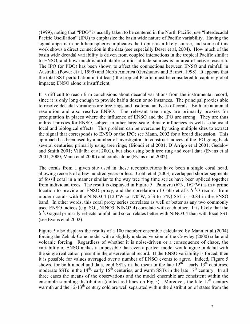
The corals from a given site used in these reconstructions have been a single coral head,allowing records of a few hundred years or less. Cobb et al (2003) overlapped shorter segmentsof fossil coral in a manner similar to the way tree ring time series have been spliced togetherfrom individual trees. The result is displayed in Figure 5. Palmyra (6°N, 162°W) is in a primelocation to provide an ENSO proxy, and the correlation of Cobb et al’s δ18O record frommodern corals with the NINO3.4 (120°W to 170°W, 5°S to 5°N) SST is –0.84 in the ENSOband. In other words, this coral proxy series correlates as well or better as any two commonlyused ENSO indices (e.g. SOI, NINO3, NINO3.4) correlate with each other. It is likely that theδ18O signal primarily reflects rainfall and so correlates better with NINO3.4 than with local SST(see Evans et al 2002).

Figure 5 also displays the results of a 100 member ensemble calculated by Mann et al (2004)forcing the Zebiak-Cane model with a slightly updated version of the Crowley (2000) solar andvolcanic forcing. Regardless of whether it is noise-driven or a consequence of chaos, thevariability of ENSO makes it impossible that even a perfect model would agree in detail withthe single realization present in the observational record. If the ENSO variability is forced, thenit is possible for values averaged over a number of ENSO events to agree. Indeed, Figure 5shows, for both model and data, cold SSTs in the mean in the late 12th – early 13th centuries,moderate SSTs in the 14th- early 15th centuries, and warm SSTs in the late 17th century. In allthree cases the means of the observations and the model ensemble are consistent within theensemble sampling distribution (dotted red lines on Fig 5). Moreover, the late 17th centurywarmth and the 12-13th century cold are well separated within the distribution of states from the

8

model ensemble runs: one would expect the later period to be warmer than the earlier one inroughly 7 out of every 8 realizations. Applying these statistics to reality, we would expectnature’s single realization to be warmer in the later period with close to a 90% probability. Inboth data and model there is also a systematic difference in the strength of the ENSO cycle inthe two periods. There are numerous large El Niño events in the late 17th century and very fewin the 12th to early 13th century period. (This difference is statistically significant at the 0.1 levelfor both model and data.) Thus more (less) ENSO variability goes with a colder (warmer) meanSST in the eastern equatorial Pacific.

The differences -- in the model run, at least -- are a consequence of the Bjerknes mechanism.The result is, at first, counterintuitive: the warmer tropical Pacific temperatures occur at a timeof increased volcanic activity and global cooling (Crowley, 2000; Jones et al 2001) and visaversa. If there is a cooling over the entire tropics then the Pacific will change more in the westthan in the east because the strong upwelling in the east holds the temperature closer to the pre-existing value. Hence the east-west temperature gradient will weaken, so the winds willslacken, so the temperature gradient will decrease further – the Bjerknes feedback, leading to amore El Niño-like state. This chain of physical reasoning is certainly correct as far as it goes,and the agreement between the data and the simulation with the simplified Zebiak-Cane modelis evidence for the idea that the Bjerknes feedback holds sway in response to a change inradiation forcing. But the climate system is complex and processes not considered in thisargument, such as cloud feedbacks, might be controlling.

4. ENSO in the Future

Before turning to model projections of the future, we briefly consider what can be learned fromthe changes since the rise of CO2 began in earnest in the late 19th century. Trenberth and Hoar(1997), noting that greenhouse gas concentrations rose sharply in the past few decades, arguedthat the increase in the frequency and amplitude of ENSO events in the 1980s and 1990s washighly unusual, significantly different from the behavior in the preceding century, and thusattributable to anthropogenic causes. Rajagopalan et al (1997) used a different statistical modelto formulate their null hypothesis and concluded that the behavior was not significantlydifferent from that in the earlier part of the instrumental record (also see Wunsch, 1999). Thearguments are technical and inconclusive; the reader is invited to compare the last quarter ofthe 20th century with the last quarter of the 19th century in Figure 1 and decide if the level ofENSO activity in the two eras is strikingly different. By some measures the 1877 El Niño wasmore powerful than any of the events in the 20th century. Record drought in India, as well assevere droughts in Ethiopia, China, Northeast Brazil and elsewhere, all contributed to what isfairly described as a global holocaust (Davis, 2001).

We noted that the data of Cobb et al (2003) showed cooling in the eastern equatorial Pacific attimes in the past when the global climate warmed due to increased solar radiation or reducedvolcanism, a result reproduced in the modeling study of Mann et al (2004) and explained by theBjerknes feedback. However, this same relation does not seem to hold for the 20th century,when radiative forcing, global temperatures, and NINO3 SST all increase. (Crowley, 2000found the greatest disagreement between global mean temperature and a model forced by solar,volcanic and greenhouse gas variations in the early 20th century.) Perhaps this change in

9

behavior is due to the impact of atmospheric aerosol or perhaps there is something missed in ourargument when the radiative increase is due to increased greenhouse gases. Another possibilityis suggested by the result of Cane et al (1997), whose plots of temperature trends from 1900 to1991 are updated to 2000 in Fig 6. Fig. 6 shows essentially no change in the eastern centralPacific. (Cane et al found a slight cooling, but it was not significantly different from zero in theNINO3.4 region.) However, the data in this region is quite sparse, so this conclusion is notrobust. But the east-west SST gradient does become significantly stronger over the century – aswould be expected from the Bjerknes feedback (Fig 6, bottom panel).

If we are to trust a model to predict ENSO in the greenhouse world, it is necessary that itreproduces the changes in prior centuries, but it may not be sufficient. In addition to simulatingchanges, it greatly increases our confidence if the model can simulate the defining features ofthe ENSO cycle with some skill. Is the mean frequency close to 4 years? Is the largest warmanomaly where it is observed in the eastern equatorial Pacific? Does the model’s cold tongueextend too far to the west, into the warm pool region? Unfortunately, few of thecomprehensive Coupled General Circulation Models (CGCMs) get these features right.AchutaRao and Sperber (2002) reviewed the simulations of ENSO in 17 CGCMs that were partof the Coupled Model Intercomparison Project (CMIP). Most of the model El Niños were tooweak and markedly in the wrong location. Five of the models were judged to “represent wellthe Walker circulation anomalies, the warming and enhanced rainfall in the central/eastPacific.” Some of these model ENSOs had most of their power at a higher frequency (~ 2years) than observed, and most did not have the correct phase with respect to the annual cycle.

Collins et al. (2004) investigated the predictions from 20 CMIP CGCMs of changes in ENSOdue to 1% per year increases in greenhouse gases. Figure 7 summarizes the results. The toppanel shows the histogram over the 20 model results of a measure of whether the mean statebecomes more El Niño-like or more La Niña-like. The most probable outcome is no large trendin either direction. The middle panel is the histogram weighted by how well the modelsimulates ENSO in the present climate. The measure of quality used is obviously somewhatarbitrary, but the results are not very different from the unweighted histogram and would bequalitatively the same for any sensible measure. As the bottom panel shows, the models that dothe best simulations predict small changes.

The ENSO cycle depends on the seasonal cycle, as is obvious from its tendency to have apattern of evolution locked to the calendar. Few CGCMs are capable of realistic simulations ofthe climatology of the real world. This problem can be “fixed” with “flux corrections”,empirical terms added to push the model away from its own climatology toward the observedone. Such a fix raises questions as to whether or not the flux-corrected model will have thecorrect variability or the correct sensitivities to greenhouse gases. Strenuous efforts are nowmade to avoid flux corrections. Much of the difficulty models have with ENSO variability is aconsequence of their poor tropical Pacific mean climates. Rather small changes have greatconsequence, as succinctly illustrated in Collins (2000). In simulations of a 4xCO2 world, theHADCM2 model, which was flux corrected, had a stronger ENSO at a higher frequency than ina control simulation. A 4xCO2 simulation with HADCM3, an improved version of HADCM2(no flux correction, higher resolution, improved process parameterizations), showed no changein ENSO. The two models have different mean states in the control runs, and different changes

10

in the 4xCO2 world. These differences in the mean, which are primarily due to subtledifferences in the parameterization of low cloud, account for the differences in ENSO response.

Doherty and Hulme (2002) looked at the simulations from 12 CGCMs of changes in the SOIand tropical precipitation from 1900 to 2099. (Data from these 12 are available at the IPCCData Distribution Centre; many are also in the CMIP set.) They report that changes in SOIvariability are not coherent among the models, broadly consistent with Collins et al (2004).They do find an overall tendency toward a more positive SOI – a more La Niña-like state.Specifically, 6 of the simulations showed a statistically significant positive trend and 2 astatistically significant negative (El Niño-like) trend, while the remaining 4 showed nosignificant trends.

The positive trend is in keeping with expectations based on the Bjerknes feedback, but wassurprising because two of the earliest studies of ENSO in the greenhouse with this generation ofmodels reported a positive (more El Niño-like) trend in NINO3 (Timmermann et al, 1999; Caiand Whetton, 2000). Moreover, the models used in these studies, ECHAM4 and CSIRO, areamong the ones found to have positive trends in the SOI. One possible reason for thediscrepancy between the two measures of ENSO is that a trend toward more La Niña-like SSTsin the eastern Pacific is overridden by the overall global warming; it would be revealed bylooking at east-west temperature gradients instead of NINO3, as is the case for the 20th centuryobservations in Figure 6. Or, it might be that the overall pattern of the ENSO events is alteredin the greenhouse world; for example, a shift to the southeast as observed in the late 20th centuryby Kumar et al (1999). Doherty and Hulme (2002) found pattern changes in a minority of the12 simulations they considered, with HADCM2 and ECHAM4 showing eastward shifts.

Conclusions

Glendower: I can summon spirits from the vasty deep.Hotspur: why, so can I, or so can any man; but will they come when you do call forthem?Henry IV, Part 1, Act 3 Scene 1

ENSO variations impact climate world wide because the changes in the heating of the tropicalatmosphere they create alter the global atmospheric circulation. Changes in the mean state ofthe tropical Pacific would have similar impacts. Since societies and ecosystems are profoundlyaffected, we would like to know how ENSO and the mean state of the tropical Pacific willchange in our greenhouse future. We must rely on models to make such predictions, since thepast does not provide a true analogue of the new climate we are creating.. Our comprehensivecoupled general circulation models are impressive achievements, now able to simulate manyfeatures of the climate with striking verisimilitude. The ENSO cycle, however, is not theirforte. Present attempts to summon the ENSO of the future bring forth a motley and uncertainset of responses. The paleoclimate record shows us that ENSO behavior is quite sensitive toclimatological conditions, so it stands to reason that ENSO will behave differently in the future.But we can’t say how it will differ with any confidence. Indeed, the models’ consensusestimate is that it won’t change much at all.

11

There are reasons for optimism. The quality of ENSO simulations has improved dramatically inthe past decade, and further progress is likely if computing power grows adequately. Thepaleoclimate record, almost devoid of information about ENSO only 5 years ago, is expandingrapidly and even now provides enough information to test models under conditions substantiallydifferent from modern. Thus there is hope that we can soon increase our confidence in forecastsof future variability. But for the present, the future of ENSO lies in depths of vast uncertainty,beyond our summons.

Acknowledgements. Thanks to Alexey Kaplan, Naomi Naik, Amy Clement, Sandy Tudhopeand Matt Collins for valuable discussions, and to Naomi Naik and Alexey Kaplan for help withfigures and Virginia DiBlasi for help with ms preparation. This work was supported by NOAAgrants NA03OAR4310064 and NA03OAR4320179 and NSF grant ATM0347009.

REFERENCES

AchutaRao, K. and K.R. Sperber, 2002: Simulation of the El Niño Southern Oscillation:Results from the Coupled Model Intercomparision Project, Climate Dynamics, 19, 191-209.

Battisti, D.S. and AC. Hirst, 1989: Interannual variability in a tropical atmosphere-oceanmodel: influence of the basic state, ocean geometry, and nonlinearity. J. Atmos. Sci., 46,1,687-1712.

Bjerknes, J., 1969: Atmospheric teleconnections from the equatorial Pacific, Mon.Weath. Rev., 97, 163-172.

Biondi, F., A. Gershunov, and D.R. Cayan, 2001: North Pacific decadal climatevariability since 1661, Journal of Climate, 14 (1), 5-10.

Cai, W. and P.H. Whetton, 2000: Evidence for a time-varying pattern of greenhousewarming in the Pacific Ocean, Geophys. Res. Lett., 27, 2577-2580

Cane, M.A., 1986: El Niño. Annual Review of Earth and Planetary. Sci, 14, 43-70.

Cane, M.A., M. Münnich and S.E. Zebiak , 1990: A study of self-excited oscillations ofthe tropical ocean- atmosphere system. Part I: linear analysis. J. Atmos. Sci., 47, 1,562-1,577.

Cane, M.A., A.C. Clement, A. Kaplan, Y. Kushnir, R. Murtugudde, D. Pozdnyakov, R.Seager and S.E. Zebiak, 1997: 20th century sea surface temperature trends. Science,275, 957-960.

Chen, D., A. Kaplan and M.A. Cane, 2004: Application of Altimeter Observations toTropical Ocean Modeling and Climate Prediction, Intermat. J. of Remote Sensing, 22,2621-2626.

12

Clement, A.C., M.A. Cane and R. Seager, 2001: An orbitally driven tropical source forabrupt climate change. J. Climate, 14, 11, 2,369-2,375.

Clement, A., R. Seager and Mark A. Cane, 2000: Suppression of El Niño during the mid-holocene by changes in the earth’s orbit, Paleoceanogr., 15, 731-737.

Cobb, K.M., C.D. Charles, R.L. Edwards, H. Cheng, and M. Kastner, 2003: El Niño-Southern Oscillation and tropical Pacific climate during the last millennium, Nature 424,271-276.

Collins, M., 2000: Understanding Uncertainties in the response of ENSO to GreenhouseWarming. Geophys. Res. Letts., 27(21), 3509-3513.

Collins, M. and the CMIP Modelling Groups 2004: El Niño or La Niña –likeclimate change? Geophys Res Lett. Submitted.Crowley, T.J., 2000: Causes of Climate Change Over the Past 1000 years, Science, 289,270-277.

D'Arrigo, R., R. Villalba, and G. Wiles, Tree-ring estimates of Pacific decadal climatevariability, Climate Dynamics, 18, 219-224, 2001.

Doherty, R. and M. Hulme, 2002: The relationship between the SOI and the extendedtropical precipitation in simulations of future climate change. Geophys. Res. Letts.,29(10), 1475, 10.1029/2001GLO14601.

Davis, M., 2001: Late Victorian Holocausts: El Nino Famines and the Making of theThird World. Verso Press, London/New York 465 pp.

Deser, C., A.S. Phillips and J.W. Hurrell, 2004: Pacific Interdecadal Climate Variability,Linkages between the Tropics and North Pacific during boreal winter since 1900. J.Climate, submitted.

Evans, M.N., A. Kaplan and M.A. Cane, 2000: Intercomparison of coral oxygen isotopedata and historical SST: Potential for coral-based SST field reconstructions.Paleoceanogr. 15, 551-563.

Evans, M. N., M. A. Cane, D. P. Schrag, A. Kaplan, B. K. Linsley, R. Villalba, G. M.Wellington, 2001: Support for tropically-driven Pacific decadal variability based onpaleoproxy evidence, Geophysical Research Letters, 28 (19), 3689-3692.

Evans, M. N., A. Kaplan, and M.A. Cane, 2002: Pacific sea surface temperature fieldreconstruction from coral d18O data using reduced space objective analysis,Paleoceanography, 17 (1), 10.1029/2000PA000590.

Federov, A.V. and S.G. Philander, 2000: Is El Niño Changing? Science, 288, 1,997-2,002.

13

Fedorov, A.V. and Philander, S.G.H. 2001: A stability analysis of tropical Ocean-Atmosphere Interactions (Bridging Measurements of, and Theory for El Niño).J.Climate, 14, 3086-3101.

Garreaud, R.D. and D.S. Battisti, 1999: Interannual and interdecadal variability of thetropospheric circulation in the Southern Hemisphere. J. Climate, 12, 2113-2123.

Gedalov, Z., and D.J. Smith, Interdecadal climate variability and regime-scale shifts inPacific North America, Geophysical Research Letters, 28 (8), 1515-1518, 2001.

Gershunov, A. and T.P.Barnett. 1998: Interdecadal modulation of ENSOteleconnections Bull Amer. Met. Soc,. 79, 2715-2725.

Goddard, L., 2004: El Niño: Catastrophe or opportunity? J. Climate, submitted.

Goddard, L., S.J. Mason, S.E. Zebiak, C.F. Ropelewski, R. Basher and M.A. Cane, 2001:Current approaches to seasonal to interannual climate predictions. International J. ofClimatology, 21, 1,111-1,152.

Hughen, K.A., D.P. Schrag, S.B. Jacobsen, and W. Hantoro, 1999: El Niño During theLast Interglacial Period Recorded by a Fossil Coral from Indonesia, Geophys. Res. Lett.26, 3129-3132.

Jones, P.D., T.J. Osborn, and K.R. Briffa, 2001: The Evolution of Climate over the LastMillenium , Science, 292, 662-667.

Kaplan, A., M., A. Cane, Y. Kushnir, A. C. Clement, B. Blumenthal, and B.Rajagopalan, 1998: Analyses of global sea surface temperature, 1856 - 1991, J. Geophys.Res., 103, 18,567-18,589.

Koutavas, A., J. Lynch-Stieglitz, T. M. Marchitto, and J. P. Sachs, 2002: El Nino-likepatter in ice age tropical Pacific sea surface temperature, Science, 297, 226-230.

Kumar, K., B. Rajagopalan and M.A. Cane, 1999: On the weakening relationshipbetween the Indian Monsoon and ENSO. Science, 284, 2,156-2,159.

Latif, M., R. Kleeman and C. Eckert, 1997: Greenhouse warming, decadal variability, orEl Niño? AN attempt to understand the anomalous 1990s. J. Climate., 11, 2325-1339.

Mann, M.E., R.S. Bradley and M.K. Hughes, 2000: Long-Term Variability in the ElNiño/Southern Oscillation and Assocciated Teleconnections, in “El Niño and theSouthern Oscillation. Multiscale Variability and Global and Regional Impacts. Eds. byHenry F. Diaz and Vera Markgraf, Cmbridge University Press.

Mann, M.E. 2002, The Value of Multiple Proxies, Science, 297, 1481-1482.

14

Mann, M.E., M.A. Cane, S.E. Zebiak and A. Clement, 2004: Volcanic and solar forcingof El Niño over the past 100 years. J. Climate, accepted.

Mantua, N.J., S.R. Hare, Y. Zhang, J.M. Wallace, and R.C. Francis, 1997: A Pacificinterdecadal oscillation with impacts on salmon production, Bulletin of the AmericanMeteorological Society, 78, 1069-10079.

Moy, C. M., G. O. Seltzer, D. T. Rodbell, and D. M. Anderson, 2002: Variability of ElNiño/Southern Oscillation activity at millennial timescales during the Holocene epoch,Nature, 420, 162-165.

Otto-Bleisner, B.L., E.C. Brady, S-I Shin, Z. Liu, and C. Shields, 2003: Modeling ElNiño and its tropical teleconnections during the last glacial-interglacial cycle, Geophys.Res. Lett., 30, 2198, doi: 10.1029/2003GL018553.

Power, S., T. Casey, C. Folland, A. Colman, and V. Mehta, 1999: Inter-decadalmodulation of the impact of ENSO on Australia, Climate Dynamics, 15 (5), 319-324.

Rajagopalan, B., U. Lall, and M.A. Cane, 1997: Anomalous ENSO Occurrences: AnAlternate View, J. Climate., 10, 3251-2357.

Rodbell, D., G. Seltzer, D. Anderson, M. Abbott, D. Enfield, and J. Newman, 1999. An15,000 year record of El Niño-driven alluviation in southwestern Ecuador. Science, 283,516-520.

Sandweiss, D., J. Richardson, E. Reitz, H. Rollins, 1996. Geoarchaeological evidencefrom Peru for a 5000 year B.P. onset of El Niño. Science, 273, 1,531-1,533.

Timmermann, A., J. Oberhuber, A. Bacher, M. Esch, M. Latif, E. Roeckner, 1999.Increased El Niño frequency in a climate model forced by future greenhouse gaswarming, Nature, 398, 694-696.

Trenberth, K.E., and T.J. Hoar, 1997. El Niño and climate change, Geophys. Res. Lett.,24, 3057-3060.

Tudhope, A.W., C.P. Cilcott, M.T. McCulloch, E.R. Cook, J. Chappell, R.M. Ellam,D.W. Lea, J.M. Lough and G.B. Shimmield, 2001. Variability in the El Niño-SouthernOscillation Through a Glacial-Interglacial Cycle. Science, 291, 1511–1517.

Villalba, R., R.D. D'Arrigo, E.R. Cook, G.C. Jacoby, and G. Wiles, 2001. Decadal-scaleclimate variability along the extratropical western coast of the Americas: Evidence fromtree-ring records, in Interhemispheric Climate Linkages, edited by V. Markgraf, pp. 155-172, Academic Press, San Diego.

15

Wunsch, C., 1999: The interpretation of short climate records, with comments on theNorth Atlantic and Southern Oscillations. Bull. Amer. Met. Soc., 80, 245-255.

Zebiak, S.E. and M.A. Cane, 1987: A model El Niño/Southern Oscillation, Mon.Weather Rev,. 115, 2262-2278.

Zhang, Y., J.M. Wallace, and D.S. Battisti, 1997: ENSO-like interdecadal variability:1900-93, J.Climate,10, 1004-1020.

16

Figures

1. Measures of El Niño and of the Southern Oscillation, 1866-2003. The red curveis a commonly used index of El Niño, the sea surface temperature (SST) anomalyin the NINO3 region of the eastern equatorial Pacific (90°W-150°W, 5°S-5°N).The blue curve is the sea level pressure (SLP) at Darwin, Australia, an index ofthe atmospheric Southern Oscillation. The close relationship between the twoindices is evident. (Departures in the earliest part of the record are more likelydue to data quality problems than to real structural changes in ENSO.)

2. Schematics of Normal Conditions and El Niño Conditions in the equatorialPacific Ocean and atmosphere to illustrate the Bjerknes feedback. In the“normal” state, the thermocline is near the surface in the east and temperaturesthere are cold. The easterly trades are strong. The stronger winds pull thethermocline up and increase upwelling; the stronger east-west sea surfacetemperature (SST) gradient creates a stronger east west sea level pressure (SLP)gradient (a more positive Southern Oscillation), that drives stronger winds. In theEl Niño state, the winds relax, the thermocline deepens in the east and thetemperatures there warm. The SST and SLP gradients decease, weakening thetrade winds, and the warm state is reinforced.

3. The evolution of the ENSO cycle, illustrating the delayed oscillator mechanismand the Bjerknes feedback. The field indicates thermocline displacement and thearrow wind stress. See text for an explanation. The figures derive from animplementation of the model of Cane, Munnich, and Zebiak (1990). Briefly, ashallow water rectangular ocean on an equatorial beta plane is driven by a wind ofthe form A exp(µ y2/2) over the middle 30% of the basin. The amplitude Adepends on the thermocline depth at the eastern end of the equator, a proxy for theSST gradient. The model may be run at <http://ocp.ldeo.columbia.edu/enso/>

4. P!a!l!e!o!-!E!N!S!O! !v!a!r!i!a!b!i!l!i!t!y! !f!r!o!m! !fossil !c!o!r!a!l!s. From Tudhope et al (2001)!.! !(!A!)! !L!e!f!t!h!a!n!d! !side: !S!e!a!s!o!n!a!l! !r!e!s!o!l!u!t!i!o!n! !(!t!h!i!n! !l!i!n!e!s!)! !a!n!d! !2!.!2!5! !y!e!a!r! b!i!n!o!m!i!a!l! !f!i!l!t!e!r!e!d! !(!t!h!i!c!k!!l!i!n!e!s!)! !s!k!e!l!e!t!a!l! δ18O !r!e!c!o!r!d!s! !f!r!o!m! !! fossil !c!o!r!a!l!s! from the Huon Peninsula!,! !w!i!t!h! !t!h!e!!r!e!c!o!r!d! !f!r!o!m! !mod!e!r!n !c!o!r!a!l! !D!T!9!1!-!7! !s!h!o!w!n! !f!o!r! !c!o!m!p!a!r!i!s!o!n!.! !R!i!g!h!t! !h!a!n!d! !s!i!d!e!:! !2!.!5!-!7!y!e!a!r! !(!E!N!S!O!)! !b!a!n!d!p!a!s!s! !f!i!l!t!e!r!e!d! !c!o!r!a!l! δ18O t!i!m!e!s!e!r!i!e!s!.! !(!B!)! S!t!a!n!d!a!r!d! !d!e!v!i!a!t!i!o!n! !o!f!!t!h!e! !2!.!5!-!7! !y!e!a!r! !(!E!N!S!O!)! !b!a!n!d!p!a!s!s! f!i!l!t!e!r!e!d! !t!i!m!e!s!e!r!i!e!s! !o!f! !a!l!l! !m!o!d!e!r!n! !a!n!d! !f!o!s!s!i!l! !c!o!r!a!l!s!!shown in (A)!.! !A!n! !a!s!t!e!r!i!s!k! !a!f!t!e!r! !t!h!e! !c!o!r!a!l! !l!a!b!e!l! !i!n!d!i!c!a!t!e!s! !t!h!a!t! !t!h!e! t!i!m!e!s!e!r!i!e!s! !i!s! !<! !3!0!!y!e!a!r!s! !l!o!n!g!.! !T!h!e! !h!o!r!i!z!o!n!t!a!l! !d!a!s!h!e!d! !l!i!n!e!s! i!n!d!i!c!a!t!e! !m!a!x!i!m!u!m! !a!n!d! !m!i!n!i!m!u!m! !v!a!l!u!e!s!!o!f! !s!t!a!n!d!a!r!d! !d!e!v!i!a!t!i!on f!o!r! !s!l!i!d!i!n!g! !3!0!-!y!e!a!r! i!n!c!r!e!m!e!n!t!s! !i!n! !t!h!e! !m!o!d!e!r!n! !c!o!r!a!l! !r!e!c!o!r!d!s!.

5. After Mann et al (2004). Comparison of the ensemble annual mean Niño3response to the combined volcanic and solar radiative forcing over the intervalAD 1000-1999. a) Response (red--anomaly in oC relative to AD 1000-1999 mean)to radiative forcing (blue) based on an ensemble of 100 realizations. b)

17

Comparison of model ensemble-mean Niño3 (gray--anomaly in oC relative to AD1950-1980 reference period; 40 year smoothed values shown by thick marooncurve) with reconstructions of ENSO behavior from Palmyra coral oxygenisotopes (blue--the annual means of the published monthly isotope data areshown). The coral data are scaled so that the mean agrees with the model (seeMann et al (2004) for details). Warm-event (cold-event) conditions associatedwith negative (positive) isotopic departures. Thick dashed lines indicate averagesof the scaled coral data for the three available time segments (blue) and theensemble-mean averages from the model (red) for the corresponding timeintervals. The associated inter-fourth quartile range for the model means (theinterval within which the mean lies for 50% of the model realizations) is alsoshown. The ensemble mean is not at the center of this range, due to the skewednature of the underlying distribution of the model Niño3 series. Also shown(green curve) is the 40 year smoothed model result based on the response tovolcanic forcing only, with the mean shifted to match that of the coral segments.

6. (a) The trend in monthly mean SST anomalies from 1900 to 2000 in °C percentury. Updated from Cane et al (1997) Regions that cool, such as the easternequatorial Pacific, are significantly different from the mean global SST warmingof 0.4°C per century. (b) Time series of: (top) the average SST anomaly in theWP region (120°E to 160°E; 5°N to 5°S); (middle) average SST anomaly in theNINO3.4 region (120°W to 170°W; 5°N to 5°S); (bottom) the difference WP-NINO3.4, a measure of the zonal SST gradient. The linear trends in the 3 timeseries (°C per century) are 0.41±0.06, -0.08±0.25, and 0.50±0.25, respectively.

7. (a) Un-weighted histogram of a measure of ENSO (called “ENSOness” in Collinset al (2004)) of the pattern of climate change in the CMIP 1%/year increase ofgreenhouse gas experiments. The histogram is normalized to give probabilityvalues. A bin size of 0.5 is used with bins centered on 0, +/-0.5, +/-1, etc. (b)Histogram of “ENSOness” weighted by the ENSO Simulation Index (ESI), ameasure of the realism of the model control run ENSO cycle. Bin sizes etc. as in(a). (c) ENSOness measure against ESI for the CMIP models. Those models withthe more realistic ENSO cycle tend to have a smaller amplitude trend towardseither El Niño-like or La Niña-like change. From Collins et al (2004).

a

b

c

d

e

1000 1200 1400 1600 1800 2000

-0.2

0

0.2

0.4

0.6

0.8

YEAR (AD)

Nin

o3 in

dex

(oC

)

Figure 11. (a) Un-weighted histogram of the “ENSOness” of the pattern of climate change in the CMIP 1%/year experiments. The ENSOness is defined as the average of the βSAT , βMSLP and βprecip for each model (fig 10) and the histogram is normalized to give probability values. A bin size of 0.5 is used with bins centered on 0, +/-0.5, +/-1, etc. (b) Histogram of ENSOness weighted by the ENSO Simulation Index (ESI), a measure of the realism of the model control run ENSO cycle (see eq. 1). Bin sizes etc. as in (a). (c) ENSOness measure against ESI for the CMIP models. Those models with the more realistic ENSO cycle tend to have a smaller amplitude trend towards either El Niño-like or La Niña-like change.

25