the-eye.eu library...process measurement and control. he has a diploma in electronics and...
TRANSCRIPT


Python 2.6 Graphics Cookbook
Over 100 great recipes for creating and animating graphics using Python
Mike Ohlson de Fine
BIRMINGHAM - MUMBAI

Python 2.6 Graphics Cookbook
Copyright © 2010 Packt Publishing
All rights reserved. No part of this book may be reproduced, stored in a retrieval system, or transmitted in any form or by any means, without the prior written permission of the publisher, except in the case of brief quotations embedded in critical articles or reviews.
Every effort has been made in the preparation of this book to ensure the accuracy of the information presented. However, the information contained in this book is sold without warranty, either express or implied. Neither the author, nor Packt Publishing, and its dealers and distributors will be held liable for any damages caused or alleged to be caused directly or indirectly by this book.
Packt Publishing has endeavored to provide trademark information about all of the companies and products mentioned in this book by the appropriate use of capitals. However, Packt Publishing cannot guarantee the accuracy of this information.
First published: November, 2010
Production Reference: 1181110
Published by Packt Publishing Ltd. 32 Lincoln Road Olton Birmingham, B27 6PA, UK.
ISBN 978-1-849513-84-5
www.packtpub.com
Cover Image by Asher Wishkerman ([email protected])
Credits
AuthorMike Ohlson de Fine
ReviewersFlavio Barbosa
Michael Driscoll
Warren Noronha
Acquisition EditorDilip Venkatesh
Development EditorMeeta Rajani
Technical EditorGauri Iyer
IndexerTejal Daruwale
Editorial Team LeaderMithun Sehgal
Project Team LeaderAshwin Shetty
Project CoordinatorMichelle Quadros
Proofreader
Mario Cecere
GraphicsNilesh R. Mohite
Production Coordinator Aparna Bhagat
Cover WorkAparna Bhagat
About the Author
Mike Ohlson de Fine is a graduate Electrical Engineer specializing in industrial process measurement and control. He has a Diploma in Electronics and Instrumentation from Technikon Witwatersrand, an Electrical Engineering degree from the University of Cape Town, and a Masters in Automatic Control from Rand Afrikaans University. He has worked for mining and mineral extraction companies for the last 30 years. His first encounter with computers was learning Fortran 4 using punched cards on an IBM 360 as an undergraduate. Since then, he has experimented with Pascal, Forth, Intel 8080 Assembler, MS Basic, C, and C++, but was never satisfied with any of these. Always restricted by corporate control of computing activities, he encountered Linux in 2006 and Python in 2007 and became free at last.
As a working engineer he needs tools that facilitate the understanding and solution of industrial process control problems using simulations and computer models of real processes. Linux and Python proved to be excellent tools for these challenges. When he retires he would like to be part of setting up a Free and Open Source engineering virtual workshop for his countrymen and people in other poor countries to enable the bright youngsters of these countries to be intellectually free at last.
His hobbies are writing computer simulations, paddling kayaks in wild water, and surf skiing in the sea.
At the top of the pyramid of people who have helped and encouraged me to write this book is my wonderful wife Suzanne. Thank you Suzy, with all my heart. I want to dedicate this book also to three courageous people, Genevieve, Candace, and Peter, who have bravely chosen a steep and difficult path in their lives. I salute you. Next who I would like to thank are the very professional and pleasant staff of PACKT Publishing. A special thanks to the restrained and long suffering reviewers Mike Driscoll, Warren Noronha, and Flavio Barbosa. Your criticism was invaluable.

About the Reviewers
Michael Driscoll has been programming Python since 2006 and has dabbled in other languages since the late nineties. He graduated from university with a Bachelors in Science degree, majoring in Management Information Systems. Michael enjoys programming for fun and profit. His hobbies include Biblical apologetics, blogging about Python at http://www.blog.pythonlibrary.org/ and learning photography. Michael currently works for local government where he programs with Python as much as possible. Michael was also a technical editor for Python 3: Object Oriented Programming by Dusty Phillips.
I would like to thank my brothers for their support and the fun times they share with me and my dad for his indirect support. Most of all, I want to thank Jesus for saving me from myself.
Warren Noronha is an entrepreneur and geek. Computers have been part of Warren’s life since he was four years old. He began his career as a system administrator, but ended up doing everything from security and design to product development. He enjoys managing people as much as he does managing code or machines. Having worked with small startups as well as Fortune 500 companies, Warren is also a staunch supporter of free software and free speech. He has been a frequent speaker at various colleges and events, discussing subjects ranging from technology and media to launching a startup.
Warren loves working with new technologies; a trait which lead him to become one of the first users of GNU/Linux, Drupal, and Ruby on Rails, much before they grew exponentially and became mainstream technologies. He spends his time working on databases, distributed computing, social computing, and enjoys using internet and communication technology to bridge the digital divide.


Table of ContentsPreface 1Chapter 1: Start your Engines 5
Introduction 5Running a shortest Python program 6Ensuring that the Python modules are present 7A basic Tkinter program 9Make a compiled executable under Windows and Linux 11
Chapter 2: Drawing Fundamental Shapes 15Introduction 16A straight line and the coordinate system 17Draw a dashed line 18Lines of varying styles with arrows and endcaps 20A two segment line with a sharp bend 22A line with a curved bend 23Drawing intricate shapes – the curly vine 24Draw a rectangle 27Draw overlapping rectangles 28Draw concentric squares 30A circle from an oval 32A circle from an arc 34Three arc ellipses 35Polygons 36A star polygon 37Cloning and resizing stars 39
Chapter 3: Handling Text 43Introduction 43Simple text 43

ii
Table of Contents
Text font type, size, and color 45Alignment of text – left and right justify 49All the fonts available on your computer 54
Chapter 4: Animation Principles 57Introduction 57Static shifting of a ball 58Time-controlled shifting of a ball 59Complete animation using draw-move-pause-erase cycles 62More than one moving object 63A ball that bounces 65Bouncing in a gravity field 67Precise collisions using floating point numbers 70Trajectory tracing and ball-to-ball collisions 72Rotating line 76Trajectory tracing on multiple line rotations 78A rose for you 82
Chapter 5: The Magic of Color 85Introduction 85A limited palette of named colors 86Nine ways of specifying color 90A red beachball of varying hue 91A red color wedge of graded hue 94Newton's grand wheel of color mixing 96The numerical color mixing matching palette 101The animated graded color wheel 106Tkinter's own color picker-mixer 110
Chapter 6: Working with Pictures 113Opening an image file and discovering its attributes 114Open, view, and save an image in a different file format 117Image format conversion for JPEG, PNG, TIFF, GIF, BMP 118Image rotation in the plane of the image 120Image size alteration 121Correct proportion image resizing 123Separating one color band in an image 124Red, green, and blue color alteration in images 125Slider controlled color manipulation 127Combining images by blending 130Blending images by varying percentages 131Make a composite image using a mask image 132

iii
Table of Contents
Offset (roll) image horizontally and vertically 134Flip horizontally, vertically, and rotate 134Filter effects: blur, sharpen, contrast, and so on 135
Chapter 7: Combining Raster and Vector Pictures 139Simple animation of a GIF beach ball 140The vector walking creature 141Bird with shoes walking in the Karroo 145Making GIF images with transparent backgrounds using GIMP 149Diplomat walking at the palace 152Spider in the forest 156Moving band of images 160Continuous band of images 162Endless background 164
Chapter 8: Data In and Data Out 167Introduction 167Creation of a new file on a hard drive 168Writing data to a newly-created file 169Writing data to multiple files 169Adding data to existing files 170Saving a Tkinter-drawing shape to disk 171Retrieving Python data from disk storage 172Simple mouse input 173Storing and retrieving a mouse-drawn shape 174A mouse-line editor 177All possible mouse actions 181
Chapter 9: Exchanging Inkscape SVG Drawings with Tkinter Shapes 185Introduction 185The structure of an SVG drawing 186Tracing the shape of an image in Inkscape 189Converting an SVG path into a Tkinter Line 194
Chapter 10: GUI Construction: Part 1 199Introduction 199Widget configuration – a label 200Button focus 201The simplest push button with validation 203A data entry box 204Colored button causing a message pop-up 207Complex interaction between buttons 208Images on buttons and button packing 211

iv
Table of Contents
Grid Geometry Manager and button arrays 213Drop-down menus to select from a list 215Listbox variable selection 216Text in a window 218
Chapter 11: GUI Construction: Part 2 219Introduction 219The Grid Layout Geometry Manager 220The Pack Geometry Manager 222Radiobuttons to select one from many 223Checkbuttons (Tickboxes) to select some of many 224Key-stroke event handling 226Scrollbar 227Custom DIY controller widgets 228Organizing widgets inside frames 232
Appendix: Quick tips for running Python programs in Microsoft Windows 235
Running Python programs in Microsoft Windows 235Where will we find the windows installer? 235Do we have to use Python version 2.7? 236Why do we get "python is not recognized…"? 236
Index 239
PrefacePython 2.6 Graphics Cookbook is a collection of straightforward recipes and illustrative screenshots for creating and animating graphic objects using the Python language. This book makes the process of developing graphics interesting and entertaining by working in a graphic workspace, without the burden of mastering complicated language definitions and opaque examples.
What this book coversChapter 1, Start your Engines: This chapter explains how to acquire and install the Python interpreter, for MS Windows or Linux as well as how to verify that Python is correctly installed. This chapter explains how to create complete working programs that can be run on client computers that do not have Python installed.
Chapter 2, Drawing Fundamental Shapes: This shows how to create all the fundamental graphic elements including lines, circles, ovals, rectangles, polygons, and complex curves. Simple examples are provided to demonstrate how to draw the elementary shapes. The examples also provide a ready for reference for later use.
Chapter 3, Handling Text: This chapter demonstrates how to control font size, color, and position using any of the font typefaces installed on the specific operating system being used. A simple means of discovering and demonstrating all available fonts on the operating system is shown.
Chapter 4, Animation Principles: This chapter starts with examples of simple sequences of a circle in different positions and systematically progresses to smoothly-moving animations of elastic balls bouncing inside a gravity field.
Chapter 5, The Magic of Color: This chapter begins with the assembling of color palettes using color names recognizable to Python. The way colors are constructed using numbers to mix controlled amounts of red, green, and blue is explained. Tools for matching colors to any sample are constructed. This chapter demonstrates how to vary shadings of one color into another.
Dow
nlo
ad fro
m W
ow
! eBook
<w
ww
.wow
ebook.
com
>

Preface
�
Chapter 6, Working with Pictures: This chapter reveals how to acquire and use the Python Imaging Library to manipulate photo images. It also shows methods of image format conversion, re-sizing, rotating, color transforming, and complex filtering.
Chapter 7, Combining Vector and Raster Images: This chapter demonstrates the ways of combining animated vector graphics with photographic images to produce complex animations.
Chapter 8, Data in and Data Out: This chapter starts with basic storing and retrieving of files to a hard drive and progresses to the construction of programs that are tools for creating, storing, and retrieving free-form shapes drawn using a mouse.
Chapter 9, Exchanging Inkscape SVG Drawings with Tkinter Shapes: This chapter shows in detail how to use the Inkscape drawing tool to convert shapes traced from a photographic image into a sequence of points which reproduce the shape in Python. Once a line is expressed as a Python sequence, it can be transformed numerically in many ways.
Chapter 10, GUI Construction: Part 1: This chapter provides basic examples of how to create buttons, data entry boxes, drop-down menus, list-boxes, and text labels. It also covers how to customize button appearance.
Chapter 11, GUI Construction: Part 2: Here the Grid Layout Manager and the Pack Layout Manager are explained and demonstrated. Examples of radio buttons, check buttons, scrollbars, frames, and keystroke event coding are given. It also shows how to construct widgets using graphic elements on a canvas.
Appendix, Quick tips for running Python programs in Microsoft Windows: This gives explanations of how to overcome some of the difficulties a new python programmer might encounter when trying to use Python in Windows.
What you need for this bookTo run the code in this book, the reader will need a Linux operating system or Microsoft Windows, and some way of downloading Python, the Python Imaging Library, and Inkscape from the internet. All these applications are free and open source. The code has been developed on Linux Ubuntu version 9.04, Microsoft Windows XP, and Windows 7.
Who this book is forThis book is for Python programmers wanting simple, clear examples of graphic programming using Python. The examples are aimed at anyone wanting to use graphic elements and images inside Python programs with the minimum of complexity. The intended reader ranges from scholars and teachers to engineers and technicians.
Preface
�
ConventionsIn this book, you will find a number of styles of text that distinguish between different kinds of information. Here are some examples of these styles, and an explanation of their meaning.
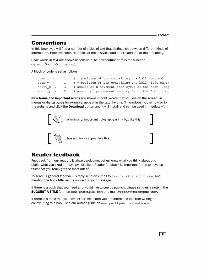
Code words in text are shown as follows: "The new feature here is the function detect_Wall_Collision()."
A block of code is set as follows:
posn_x = 1 # x position of box containing the ball (bottom)posn_y = 1 # y position of box containing the ball (left edge)shift_x = 3 # amount of x-movement each cycle of the 'for' loopshift_y = 2 # amount of y-movement each cycle of the 'for' loop
New terms and important words are shown in bold. Words that you see on the screen, in menus or dialog boxes for example, appear in the text like this: "In Windows, you simply go to the website and click the Download button and it will install and can be used immediately".
Warnings or important notes appear in a box like this.
Tips and tricks appear like this.
Reader feedbackFeedback from our readers is always welcome. Let us know what you think about this book—what you liked or may have disliked. Reader feedback is important for us to develop titles that you really get the most out of.
To send us general feedback, simply send an e-mail to [email protected], and mention the book title via the subject of your message.
If there is a book that you need and would like to see us publish, please send us a note in the SUGGEST A TITLE form on www.packtpub.com or e-mail [email protected].
If there is a topic that you have expertise in and you are interested in either writing or contributing to a book, see our author guide on www.packtpub.com/authors.

Preface
�
Customer supportNow that you are the proud owner of a Packt book, we have a number of things to help you to get the most from your purchase.
Downloading the example code for this book
You can download the example code files for all Packt books you have purchased from your account at http://www.PacktPub.com. If you purchased this book elsewhere, you can visit http://www.PacktPub.com/support and register to have the files e-mailed directly to you.
ErrataAlthough we have taken every care to ensure the accuracy of our content, mistakes do happen. If you find a mistake in one of our books—maybe a mistake in the text or the code—we would be grateful if you would report this to us. By doing so, you can save other readers from frustration and help us improve subsequent versions of this book. If you find any errata, please report them by visiting http://www.packtpub.com/support, selecting your book, clicking on the errata submission form link, and entering the details of your errata. Once your errata are verified, your submission will be accepted and the errata will be uploaded on our website, or added to any list of existing errata, under the Errata section of that title. Any existing errata can be viewed by selecting your title from http://www.packtpub.com/support.
PiracyPiracy of copyright material on the Internet is an ongoing problem across all media. At Packt, we take the protection of our copyright and licenses very seriously. If you come across any illegal copies of our works, in any form, on the Internet, please provide us with the location address or website name immediately so that we can pursue a remedy.
Please contact us at [email protected] with a link to the suspected pirated material.
We appreciate your help in protecting our authors, and our ability to bring you valuable content.
QuestionsYou can contact us at [email protected] if you are having a problem with any aspect of the book, and we will do our best to address it.

1Start your Engines
In this chapter, we will cover:
The Shortest Python Program
Ensure the Python Modules are present
A Basic Python GUI in Tkinter
Make a Compiled Executable under Linux
Make a Compiled Executable under MS Windows
IntroductionThis book is a collection of code recipes for creating and animating graphic objects using the marvelous Python language. In order to create and manipulate graphic objects, Python makes use of the Tkinter module. The prerequisite for using Python and Tkinter is obviously to have both installed. Both are free and Open Source and instructions for obtaining and installing them are abundantly available on the web. Just Google phrases like "install Python" and you will be spoilt for choice.
Our first task is to prove that Python and Tkinter are installed and working on our computer. In this book, we use Python version 2.6. Python 3.0 which came out in 2010 requires some changes in syntax that we won't be using in this book.
Let's look at some simple tests to check if Python is installed. If we download and install Python on Windows, it automatically includes Tkinter as one of the essential modules so we do not need to acquire and install it separately.

Start your Engines
6
Running a shortest Python programWe need a one line Python program that will prove that the Python interpreter is installed and working on our computer platform.
How to do it...1. Create a folder (directory) called something like construction_work or constr
for short. You will place all your Python programs inside this directory. In a text editor such as gedit on Linux or notepad on Windows. If we are working in Windows, there is a nice editor called "Context" that can be downloaded for free from http://www.contexteditor.org/ Context, that is sensitive to Python syntax and has a search-and-replace function that is useful.
2. Type the following line:Print 'My wereld is "my world" in Dutch'
3. Save this as a file named simple_1.py, inside the directory called constr.
4. Open up an X terminal or a DOS window if you are using MS Windows.
5. Change directory into constr - where simple_1.py is located.
6. Type python simple_1.py and your program will execute. The result should look like the following screenshot:
7. This proves that your Python interpreter works, your editor works, and that you understand all that is needed to run all the programs in this book. Congratulations.
"""Program name: simplest_1.pyObjective: Print text to the screen.
Keywords: text, simplest=========================Printed "mywereld" on terminal.Author: Mike Ohlson de Fine
"""Print 'mywereld is "my world" in Dutch'

Chapter 1
�
How it works...Any instructions you type into a Linux X terminal or DOS terminal in MS Windows are treated as operating system commands. By starting these commands from within the same directory where your Python program is stored you do not have to tell the Python and operating system where to search for your code. You could store the code in another directory but you would then need to precede the program name with the path.
There's more...Try the longer version of the same basic print instructions shown in the following program.
All the text between the """ (triple quotation marks) is purely for the sake of good documentation and record keeping. It is for the use of programmers, and that includes you. Alas, the human memory is imperfect. Bitter experience will persuade you that it is wise to provide fairly complete information as a header in your programs as well as comments inside the program.
However, in the interest of saving space and avoiding distractions, these header comments have been left out in the rest of this book.
Ensuring that the Python modules are present
Here is a slightly longer version of the previous program. However, the following modules are commanded to "report for duty" inside our program even though they are not actually used at this time: Tkinter, math, random, time, tkFont.
We need the assurance that all the Python modules we will be using later are present and accessible to Python, and therefore, to our code. Each module is a self-contained library of code functions and objects that are called frequently by the commands in your programs.
How to do it...1. In a text editor type the lines given in the following code.
2. Save this as a file named simple_2.py, inside the directory called constr as we did previously.
3. As before, open up an X terminal or a DOS window, if you are using MS Windows.
4. Change directory into constr - where simple_1.py is located.

Start your Engines
�
5. Type python simple_2.py and our program should execute. The result should look like the following screenshot:
This proves that your Python interpreter can access the necessary library functions it will need."""Program name: simplest_2.pyObjective: Send more than one line of text to the screen.Keywords: text, simple======================================Author: Mike Ohlson de Fine"""import Tkinterimport mathimport randomimport timeimport tkFontprint "======================================="print "A simple, apparently useless program like this does useful things:"print "Most importantly it checks whether your Python interpreter and "print "the accompanying operating system environment works"print " - including hardware and software"print "======================================"print " No matter how simple it is always a thrill"print " to get your first program to run"
How it works...The print command is an instruction to write or print any text between quotation marks like "show these words" onto the monitor screen attached to your computer. It will also print the values of any named variables or expressions typed after print.

Chapter 1
�
For example: print "dog's name: ", dog_name. Where dog_name is the name of a variable used to store some data.
The print command is very useful when you are debugging a complicated sequence of code because even if the execution fails to complete because of errors, any print commands encountered before the error is reached will be respected. So by thoughtful placing of various print statements in your code, you are able to zero in on what is causing your program to crash.
There's more...When you are writing a piece of Python code for the first time, you are often a bit unsure if your understanding of the logic is completely correct. So we would like to watch the progress of instruction execution in an exploratory way. It is a great help to be able to see that at least part of the code works. A major strength of Python is the way it takes our instructions one at a time and executes them progressively. It will only stop when the end is reached or a when programming flaw halts progress. If we have a twenty line program and only the first five lines are bug-free and the rest are unexecutable garbage, the Python interpreter will at least execute the first five. This is where the print command is a really potent little tool.
This is how you use print and the Python interpreter. When we are having trouble with our code and it just won't work and we are battling to figure out why, we can just insert print statements at various chosen points in our program. This way you can get some intermediate values of variables as your own private status reports. When we want to switch off our print watchdogs we simply type a hash (#) symbol in front, thus transforming them into passive comments. Later on, if you change your mind and want the prints to be active again you just remove the leading hash symbols.
A basic Tkinter programHere we attempt to execute a Tkinter command inside the Python program. The Tkinter instruction will create a canvas and then draw a straight line on it.
How to do it...1. In a text editor, type the code given below.
2. Save this as a file named simple_line_1.py, inside the directory called constr again.
3. As before open up an X terminal or DOS window if you are using MS Windows.
4. Change directory into constr - where simple_line_1.py is located.

Start your Engines
10
5. Type python simple_line_1.py and your program should execute. The command terminal result should look like the following screenshot:
6. The Tkinter canvas output should look like the following screenshot:
7. This proves that your Python interpreter works, your editor works, and the Tkinter module works. This is not a trivial achievement – you are definitely ready for great things. Well done.
#>>>>>>>>>>>>>>>>>>>>>>>>>>>>>>>>>>>>>>>from Tkinter import *root = Tk()root.title('Very simple Tkinter line') canvas_1 = Canvas(root, width=300, height=200, background="#ffffff")canvas_1.grid(row=0, column=0)
canvas_1.create_line(10,20 , 50,70)root.mainloop()#>>>>>>>>>>>>>>>>>>>>>>>>>>>>>>>>>>>>>>>>
How it works...To draw a line, we only need to give the start point and the end point.
The start point is the first pair of numbers in canvas_1.create_line(10,20 , 50,70).In another way, the start is given by the coordinates x_start=10 and y_start=20. The end point of the line is specified by the second pair of numbers x_end=50 and y_end=70. The units of measurement are pixels. A pixel is the smallest dot that can be displayed on our screen.

Chapter 1
11
For all other properties like line thickness or color, default values of the create_line() method are used.
However, should you want to change color or thickness, you just do it by specifying the settings.
Make a compiled executable under Windows and Linux
How do we create and execute a.exe file that will run a compiled version of our Python and Tkinter programs? Can we make a self-contained folder that will run on an MS Windows or Linux distribution that uses a different version of Python from the ones we use? The answers to both questions are yes and the tool to achieve this is an Open Source program called cx_Freeze. Often what we would like to do is have our working Python program on a memory stick or downloadable on a network and be able to demonstrate it to friends, colleagues, or clients without the need to download Python onto the client's system. cx_Freeze allows us to create a distributable form of our Python graphic program.
Getting readyYou will need to download cx_Freeze from http://cx-freeze.sourceforge.net/. We need to pick a version that has the same version number as the Python version we are using. Currently, there are versions available from version 2.4 up to 3.1.
How to do it under MS Windows...1. MS Windows: Download cx_Freeze-4.2.win32-py2.6.msi, the windows
installer for Python 2.6. If we have another Python version, then we must choose the appropriate installer from http://cx-freeze.sourceforge.net/.
2. Save and run this installer.
3. On completion of a successful Windows install we will see a folder named cx_Freeze inside \Python26\Lib\site-packages\.
How to do it under Linux (Debian and Ubuntu)...1. In a terminal run the command apt-get install cx-freeze.
2. If this does not work we may need to first install a development-capable version of Python by running the command apt-get install python-dev. Then go back and repeat step 1.
Start your Engines
12
3. Test for success by typing in python in a command terminal to invoke the Python interpreter.
4. Then after the >>> prompt, type import cx_Freeze. If the interpreter returns a new line and the >>> prompt again, without any complaints, we have been successful.
How to compile under both Linux and MS Windows...1. If the file we want to package as an executable is named walking_birdy_1.py in
a folder called /constr, then we prepare a special setup file as follows.#setup.pyfrom cx_Freeze import setup, Executablesetup(executables=[Executable("/constr/walking_birdy_1.py")])
2. Save it as setup.py.
3. Then, in a command terminal runpython /constr/setup.py build
4. We will see a lot of system compilation commands scrolling down the command terminal that will eventually stop without error messages.
5. We will find our complete self-contained executable inside a folder named build. Under Linux, we will find it inside our home directory under /build/exe.linux-i686-2.6. Under MS Windows, we will find it inside C:\Python26\build\exe.win-py2.6.
6. We just need to copy the folder build with all its contents to wherever we want to run our self-contained program.
How it works...A word of caution. If we use external files like images inside our code, then the path addresses of the files must be absolute because they are coded into, or frozen, into the executable version of our Python program. There are ways of setting up search paths which can be read at http://cx-freeze.sourceforge.net/cx_Freeze.html.
For example, say we want to use some GIF images in our program and then demonstrate them on other computers. First we place a folder called, for example, /birdy_pics, onto a USB memory stick. In the original program, walking_birdy_1.py, make sure the path addresses to the images point to the /birdy_pics folder on the stick. After compilation, copy the folder build onto the USB memory stick. Now when we double-click on the executable walking_birdy_1 it can locate the images on the USB memory stick when it needs to. These files include everything that is needed for your program, and you should distribute the whole directory contents to any user who wants to run your program without needing to install Python or Tkinter.
Chapter 1
13
What about py2exe?There is another program called py2exe that will also create executables to run on MS Windows. However, it cannot create self-contained binary executables to run under Linux whereas cx_Freeze can.
Dow
nlo
ad fro
m W
ow
! eBook
<w
ww
.wow
ebook.
com
>


2Drawing Fundamental
Shapes
In this chapter, we will cover:
A straight line and the coordinate system
Drawing a dashed line
Lines of varying styles with arrows and endcaps
A two-segment line with a sharp bend
A line with a curved bend
Drawing intricate stored shapes - the curly vine
Drawing a rectangle
Drawing overlapping rectangles
Drawing concentric squares
A circle from an oval
A circle from an arc
Three ellipses
The simplest polygon
A star polygon
The art of cloning stars

Drawing Fundamental Shapes
16
IntroductionGraphics are all about pictures and drawings. In computer programs, a line is not drawn by a hand, holding a pencil, but by the manipulation of numbers on a screen. This chapter provides the fine-grained detail or atomic structure for the rest of the book. Here we lay down the most basic graphic building blocks in their simplest form. The most useful options are presented inside self-contained programs. You can if you want, use the code without understanding in detail how it works. You can learn by doing. You can learn by playing and play is the serious work that unskilled animals do in order to learn almost everything they need for survival.
You can cut and paste the code and it should just work without modification. The code is easily modified and you are encouraged to tinker with it and tweak the parameters inside the drawing methods. The more you tinker with it, the more you will understand.
The area of screen where lines and shapes are drawn is the canvas in Python. It is created when the Tkinter method canvas() is executed.
Central to using numbers to describe lines and shapes is a coordinate system that says where a line or shape starts and where it ends. In Tkinter, as in most computer graphic systems, the top-left is the start of the screen or canvas and bottom-right is the end – where the largest numbers describe location. This system is shown in the next figure, which is the universal computer screen coordinate system.
Chapter 2
1�
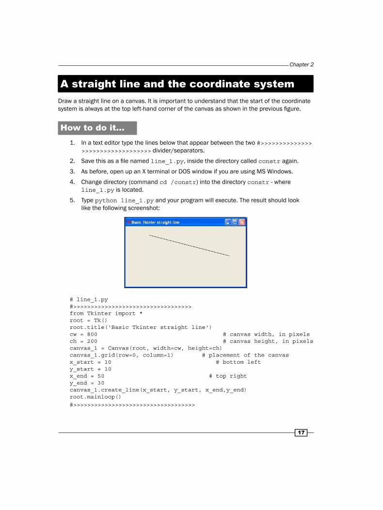
A straight line and the coordinate systemDraw a straight line on a canvas. It is important to understand that the start of the coordinate system is always at the top left-hand corner of the canvas as shown in the previous figure.
How to do it...1. In a text editor type the lines below that appear between the two #>>>>>>>>>>>>>>
>>>>>>>>>>>>>>>>>>> divider/separators.
2. Save this as a file named line_1.py, inside the directory called constr again.
3. As before, open up an X terminal or DOS window if you are using MS Windows.
4. Change directory (command cd /constr) into the directory constr - where line_1.py is located.
5. Type python line_1.py and your program will execute. The result should look like the following screenshot:
# line_1.py#>>>>>>>>>>>>>>>>>>>>>>>>>>>>>>>>>> from Tkinter import *root = Tk()root.title('Basic Tkinter straight line')cw = 800 # canvas width, in pixelsch = 200 # canvas height, in pixelscanvas_1 = Canvas(root, width=cw, height=ch)canvas_1.grid(row=0, column=1) # placement of the canvasx_start = 10 # bottom lefty_start = 10x_end = 50 # top righty_end = 30canvas_1.create_line(x_start, y_start, x_end,y_end)root.mainloop()#>>>>>>>>>>>>>>>>>>>>>>>>>>>>>>>>>>>
Drawing Fundamental Shapes
1�
How it works...We have written the coordinates for our line differently from the way we did in the previous chapter because we want to introduce symbolic assignments into the create_line() method. This is a preliminary step to making our code re-usable. There is more than one way to specify the points that define the location of line. The neatest way is to define a Python list or tuple by name and then just insert this name of the list as the argument of the create_line() method.
For example, if we wanted to draw two lines, one from (x=50, y=25) to (x= 220, y=44) and the second line between(x=11, y=22) and (x=44, y=33) then we could write the following lines in our program:
line_1 = 50, 25, 220, 44 # this is a tuple and can NEVER changeline_2 = [11, 22, 44, 33] # this is a list and can be changed anytime.canvas_1.create_line(line_1)
canvas_1.create_line(line_2)
Note that although line_1 = 50, 25, 220, 44 is syntactically correct Python, it is considered to be poor Python grammar. It is better to write line_1 = ( 50, 25, 220, 44) because this is more explicit and therefore clearer to someone reading the code. Another point to note is that canvas_1 is an arbitrary name I have given to the particular instance of a canvas of a certain size. You can give it any name you like.
There's more...Most shapes can be made up of pieces of lines joined together in a multitude of ways. An extremely useful attribute that Tkinter offers is the ability to transform sequences of straight lines into smooth curves. This attribute of lines can be used in surprising ways and is illustrated in recipe 6.
Draw a dashed lineA straight dashed line, three pixels thick is drawn.
How to do it...The instructions used in the previous example are used. The only change is in the name of the Python program. This time you should use the name dashed_line.py instead of line_1.py.
# dashed_line.py#>>>>>>>>>>>>>>>>>>>>>>>>>>>>>>>>>>>>>>>>>>>from Tkinter import *

Chapter 2
1�
root = Tk()root.title('Dashed line')cw = 800 # canvas widthch = 200 # canvas heightcanvas_1 = Canvas(root, width=cw, height=ch)canvas_1.grid(row=0, column=1)
x_start = 10y_start = 10x_end = 500y_end = 20canvas_1.create_line(x_start, y_start, x_end,y_end, dash=(3,5), width = 3)root.mainloop()#
How it works...The new things here are the addition of some style specifications for the line.
dash=( 3,5) says that there should be three solid pixels followed by five blank pixels and width = 3 specifies that the line should be 3 pixels thick.
There's more...You can specify a limitless variety of dash-space patterns. A dash-space pattern specified as dash = (5, 3, 24, 2, 3, 11) would result in a line with three patterns repeated over and over throughout the length of the line. The pattern would consist of five solid pixels followed by three blank pixels. Then there would be 24 solid pixels followed by only two blank pixels. The third variation would be three solid followed by 11 blank pixels and then the whole set of three patterns would begin again. The list of dash-blank pairs can go on as long as you like. The even-numbered length specifications will specify the length of solid pixels.
The dash attribute is quirky on different operating systems. For instance on a Linux operating system it behaves as it should by obeying the directives for line and space distances but on MS Windows there is no respect for solid-dash directives if they exceed ten pixels in size

Drawing Fundamental Shapes
20
Lines of varying styles with arrows and endcaps
Four lines are drawn in different styles. We see how attributes like color and end shape can be obtained. A Python for loop is used to make an interesting pattern using the specifications of the dash attribute. In addition the color of the canvas background has been made green.
How to do it...The instructions used in recipe 1 should be used again.
Just use the name 4lines.py when you write, save, and execute this program.
Arrows and endcaps have been introduced into the line specifications.
#4lines.py#>>>>>>>>>>>>>>>>>>>>>>>>>>>>>>>>>>>>>>>>>>>>>>from Tkinter import *root = Tk()root.title('Different line styles')cw = 280 # canvas widthch = 120 # canvas heightcanvas_1 = Canvas(root, width=cw, height=ch, background="spring \ green")canvas_1.grid(row=0, column=1)
x_start, y_start = 20, 20x_end, y_end = 180, 20canvas_1.create_line(x_start, y_start, x_end,y_end,\ dash=(3,5), arrow="first", width = 3)x_start, y_start = x_end, y_endx_end, y_end = 50, 70canvas_1.create_line(x_start, y_start, x_end,y_end,\ dash=(9,5), width = 5, fill= "red")x_start, y_start = x_end, y_endx_end, y_end = 150, 70canvas_1.create_line(x_start, y_start, x_end,y_end, \ dash=(19,5),width= 15, caps="round", \ fill= "dark blue")x_start, y_start = x_end, y_endx_end, y_end = 80, 100canvas_1.create_line(x_start, y_start, x_end,y_end, fill="purple") #width reverts to default= 1 in absence of explicit spec.root.mainloop()#>>>>>>>>>>>>>>>>>>>>>>>>>>>>>>>>>>>>>>>>>>>>>>

Chapter 2
21
How it works...To draw a line you only need to give the start point and the end point.
The preceding screenshot shows the result of execution on Ubuntu Linux
In this example we have saved a bit of work by re-using previous line position specifications. See the next two screenshots.
The preceding screenshot shows the result of execution on MS Windows XP.
There's more...Here is where you may see the difference between Linux's and MS Windows's ability to draw dashed lines using Tkinter. The solid portion of the dash was specified as 19 pixels long. On the Linux (Ubuntu9.10) platform this specification was respected but Windows disregarded the instruction.

Drawing Fundamental Shapes
22
A two segment line with a sharp bendLines do not have to be straight. A more general type of line can be made up of many straight segments joined together. You simply decide where you want the points that join sections of the multi-segment line and the order in which they should be joined.
How to do it...The instructions are the same as for recipe 1. Just use the name sharp_bend.py when you write, save, and execute this program.
Just make a list of the x,y pairs defining each point and place them in the sequence that you want them connected in. The list can be as long as you like.
#sharp_bend.py#>>>>>>>>>>>from Tkinter import *root = Tk()root.title('Sharp bend')cw = 300 # canvas widthch = 200 # canvas heightcanvas_1 = Canvas(root, width=cw, height=ch, background="white")canvas_1.grid(row=0, column=1)
x1 = 50y1 = 10x2 = 20y2 = 80x3 = 150y3 = 60
canvas_1.create_line(x1,y1, x2,y2, x3,y3)root.mainloop()
How it works...For clarity only three points have been defined: first =(x1,y1), second =(x2,y2) and third = (x3, y3). However, there is no limit to the number of sequential points that could be specified.
The preceding screenshot shows the line with a sharp bend.
Chapter 2
23
There's more...Ultimately you could have complicated figures stored as long sequences of points in files on some storage device. For example, you might want to produce something like a cartoon strip.
You could construct a library of body parts and face features seen from different angles. There could be a selection of different mouth and eye shapes. The daily chore of assembling your comic strip could be partially automated. One of the things you would need to think about would be how to scale the component parts to be larger or smaller and also how to position them in different places and even rotate them to different angles. All these ideas are developed in this book.
In particular see the next examples of how complex shapes can be stored and manipulated in a relatively compact form. The SVG (Scaled Vector Graphics) standard for drawing manipulation, particularly on web pages, uses a similar but different convention for representing shapes. Because both SVG and Tkinter are well defined it means that you can construct code for converting from one form to the other.
Examples of this are shown in Chapter 6, Working with Pictures.
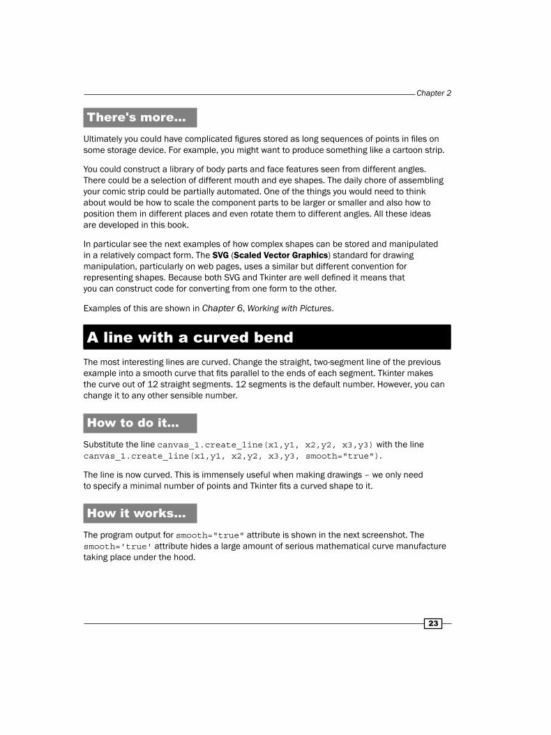
A line with a curved bendThe most interesting lines are curved. Change the straight, two-segment line of the previous example into a smooth curve that fits parallel to the ends of each segment. Tkinter makes the curve out of 12 straight segments. 12 segments is the default number. However, you can change it to any other sensible number.
How to do it...Substitute the line canvas_1.create_line(x1,y1, x2,y2, x3,y3) with the line canvas_1.create_line(x1,y1, x2,y2, x3,y3, smooth="true").
The line is now curved. This is immensely useful when making drawings – we only need to specify a minimal number of points and Tkinter fits a curved shape to it.
How it works...The program output for smooth="true" attribute is shown in the next screenshot. The smooth='true' attribute hides a large amount of serious mathematical curve manufacture taking place under the hood.
Drawing Fundamental Shapes
24
To fit a curve to a pair of intersecting lines requires the curve and the lines to run parallel at the beginning and end but in the middle an entirely different process known as spline fitting is used. The consequence of this is that this kind of curvaceous smoothing is computationally expensive and if you do too much of it your program execution slows down. This has implications for what kinds of action can be successfully animated.
There's more...What we do later is to use the curve attribute to make more pleasing and exciting shapes. Ultimately you could accumulate for yourself a library of shapes. If you did this you would be re-creating some vector graphics that are freely available from the web. Look at www.openclipart.org. The pictures which are freely downloadable from this site are in SVG (Scaled Vector Graphics) format. If you look at the code of these pictures in a text editor you will see lines of code that are vaguely similar to the way these Tkinter programs specify the points. Some techniques for extracting useful shapes from existing SVG pictures will be demonstrated in Chapter 6, Working with Pictures.
Drawing intricate shapes – the curly vineThe task here is to draw a complicated shape in such a way that you can use it as a framework to produce unlimited variety and beauty.
We start out with a pencil and paper and draw a curly growing vine shape and transfer it in the simplest and most direct way into some code that will draw it.
This is a very important example because it reveals the essential elegance of both Python and Tkinter. The central inspiring design philosophy of Python is captured in two words: simplicity and clarity. This is what makes Python one of the best computer coding languages ever conceived.
Getting readyWhen they want to create a fresh design, most graphic artists start with a pencil and paper sketch because of the uncluttered subconscious freedom it gives. For this example, a complex curve was needed – the kind of organic design used in framing pictures in antique books.
Chapter 2
25
The smooth line was drawn with a pencil on paper and marked off at roughly, evenly spaced intervals with X's. Using a millimeter marked ruler the distance from each x to the left edge and the bottom of the paper was measured approximately. High accuracy is not needed because the curved nature of the line compensates for small imperfections.
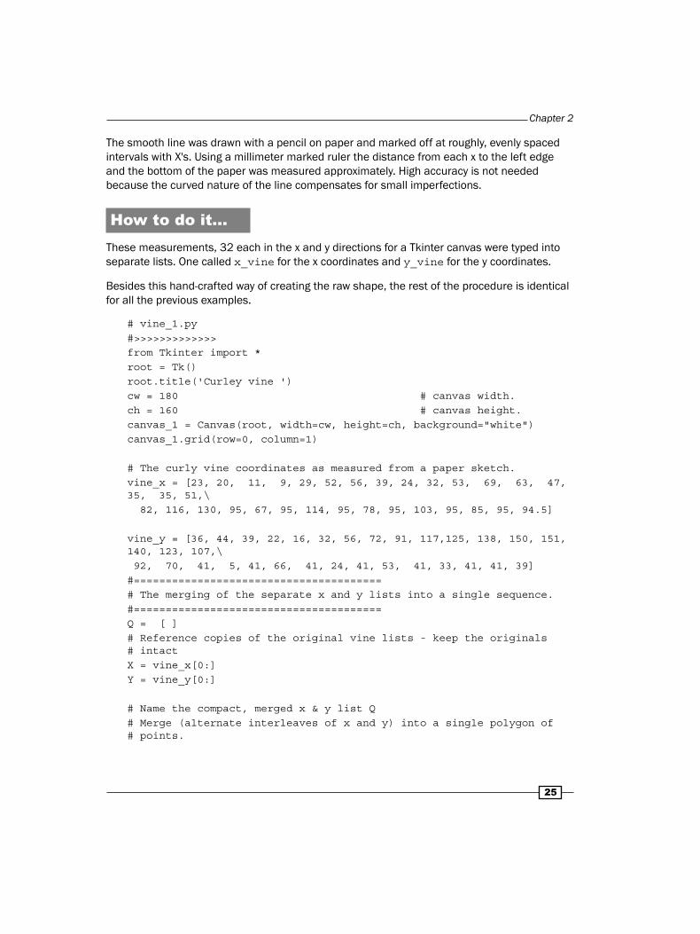
How to do it…These measurements, 32 each in the x and y directions for a Tkinter canvas were typed into separate lists. One called x_vine for the x coordinates and y_vine for the y coordinates.
Besides this hand-crafted way of creating the raw shape, the rest of the procedure is identical for all the previous examples.
# vine_1.py#>>>>>>>>>>>>>from Tkinter import *root = Tk()root.title('Curley vine ')cw = 180 # canvas width.ch = 160 # canvas height.canvas_1 = Canvas(root, width=cw, height=ch, background="white")canvas_1.grid(row=0, column=1)
# The curly vine coordinates as measured from a paper sketch.vine_x = [23, 20, 11, 9, 29, 52, 56, 39, 24, 32, 53, 69, 63, 47, 35, 35, 51,\ 82, 116, 130, 95, 67, 95, 114, 95, 78, 95, 103, 95, 85, 95, 94.5]
vine_y = [36, 44, 39, 22, 16, 32, 56, 72, 91, 117,125, 138, 150, 151, 140, 123, 107,\ 92, 70, 41, 5, 41, 66, 41, 24, 41, 53, 41, 33, 41, 41, 39]#=======================================# The merging of the separate x and y lists into a single sequence.#=======================================Q = [ ]# Reference copies of the original vine lists - keep the originals # intactX = vine_x[0:]Y = vine_y[0:]
# Name the compact, merged x & y list Q# Merge (alternate interleaves of x and y) into a single polygon of # points.

Drawing Fundamental Shapes
26
for i in range(0,len(X)): Q.append(X[i]) # append the x coordinate Q.append(Y[i]) # then the y - so they alternate and you end # with a Tkinter polygon.canvas_1.create_line(Q, smooth='true')root.mainloop()#>>>>>>>>>>>>
How it works...The result is shown in the next screenshot which is a smoothed line of 32 straight segments.
The essential trick in this task is to create a list of numbers that is in precisely the correct form to place into a create_line() method. It has to be an unbroken sequence, comma-separated, of pairs of matched x and y position coordinates of the complex curve we want to draw.
So first we create an empty list Q[] to which we are going to append alternate values of the x and y coordinates.
Because we want to leave the original lists x_vine and y_vine intact (for re-use elsewhere perhaps) we create working copies using:
X = vine_x[0:] Y = vine_y[0:]
And finally the magic interleaved merging into one list with:
for i in range(0,len(X)): Q.append(X[i]) # append the x coordinate Q.append(Y[i]) # then the y
Chapter 2
2�
The for in range() combination and the block of code following it work cyclically through the code starting at i=0, increasing one by one each until the last value len(X) is reached. Then the block of code is exited and execution continues below the block. Len(X) is a function that gives back ('returns' in programmers' parlance) the number of elements in X. Q emerges from this perfect for immediate drawing in create_line(Q).
If you leave out the smooth='true' attribute you will see the original join points that came from the original paper draw and measure process.
There's more...Some interesting effects like curling smoke, charcoal, and glowing neon are produced by copying and transforming the curly vine in various ways in Chapter 6, Working with Pictures.
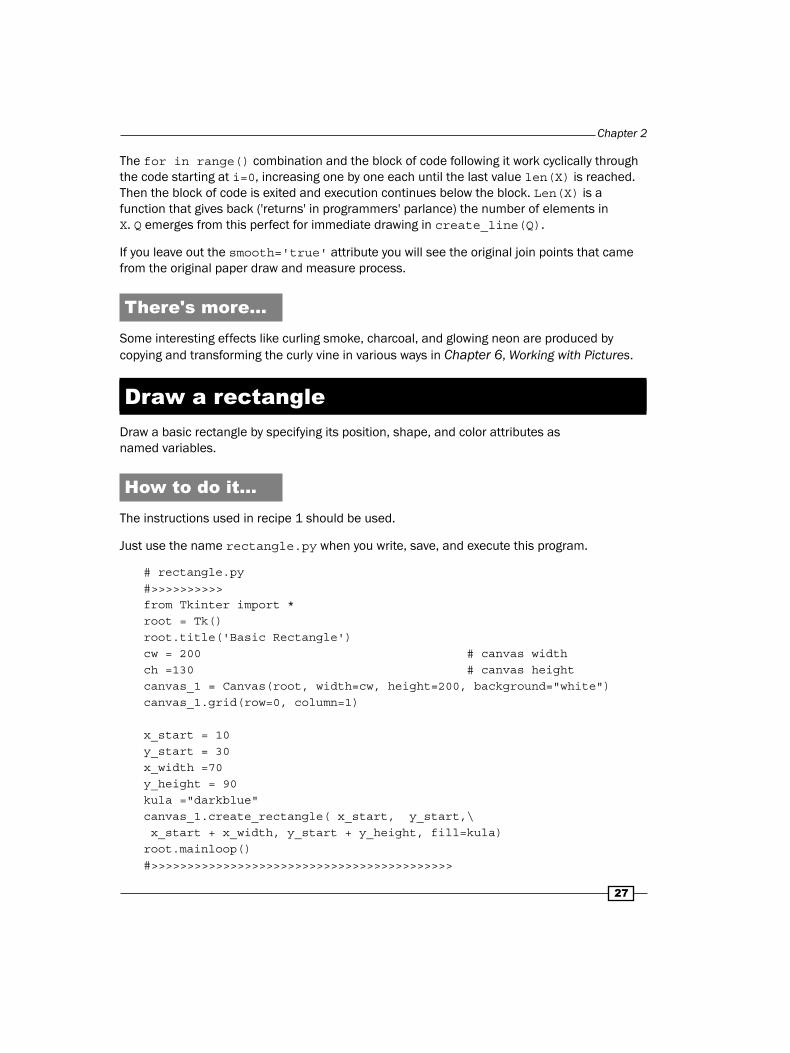
Draw a rectangleDraw a basic rectangle by specifying its position, shape, and color attributes as named variables.
How to do it...The instructions used in recipe 1 should be used.
Just use the name rectangle.py when you write, save, and execute this program.
# rectangle.py#>>>>>>>>>>from Tkinter import *root = Tk()root.title('Basic Rectangle')cw = 200 # canvas widthch =130 # canvas heightcanvas_1 = Canvas(root, width=cw, height=200, background="white")canvas_1.grid(row=0, column=1)
x_start = 10y_start = 30x_width =70y_height = 90kula ="darkblue"canvas_1.create_rectangle( x_start, y_start,\ x_start + x_width, y_start + y_height, fill=kula)root.mainloop()#>>>>>>>>>>>>>>>>>>>>>>>>>>>>>>>>>>>>>>>>>>
Dow
nlo
ad fro
m W
ow
! eBook
<w
ww
.wow
ebook.
com
>

Drawing Fundamental Shapes
2�
How it works...The results are given in the next screenshot showing a basic rectangle.
When drawing rectangles, circles, ellipses and arcs you specify the start point (the bottom-left corner) and then the end point (top-right corner) of the bounding box surrounding the figure being drawn. In the case of rectangles and squares, the bounding box coincides with the figure. But in the case of circles, ellipses, and arcs the bounding box is of course larger.
With this recipe we have tried a new way of defining the shape of the rectangle. We give the start point as [x_start, y_start] and then we just state the width and height that we want as [x_width, y_height]. This way the end point is [x_start + x_width, y_start + y_height]. This way you only need to state what the new start point is if you want to create a multiplicity of rectangles having the same height and width.
There's more...In the next example, we use a common shape to draw a series of similar but different rectangles.
Draw overlapping rectanglesDraw three overlapping rectangles by changing the numerical values defining their position, shape, and color variables.
How to do it...As before the instructions used in recipe 1 should be used.
Just use the name 3rectangles.py when you write, save, and execute this program.
# 3rectangles.py#>>>>>>>>>>>>>>>>>>>>>>>>>>>>>>>>>>>>>>>>>>> from Tkinter import *root = Tk()root.title('Overlapping rectangles')

Chapter 2
2�
cw = 240 # canvas widthch = 180 # canvas heightcanvas_1 = Canvas(root, width=cw, height=200, background="green")canvas_1.grid(row=0, column=1)
# dark blue rectangle - painted first therefore at the bottomx_start = 10y_start = 30x_width =70y_height = 90kula ="darkblue"canvas_1.create_rectangle( x_start, y_start,\ x_start + x_width, y_start + y_height, fill=kula)
# dark red rectangle - second therefore in the middlex_start = 30y_start = 50kula ="darkred"canvas_1.create_rectangle( x_start, y_start,\ x_start + x_width, y_start + y_height, fill=kula)
# dark green rectangle - painted last therefore on top of previous # ones.x_start = 50y_start = 70kula ="darkgreen"canvas_1.create_rectangle( x_start, y_start,\x_start + x_width, y_start + y_height, fill=kula)#>>>>>>>>>>>>>>>>>>>>>>>>>>>>>>>>>>>>>>>>>>>
How it works...The results are given in the next screenshot, which shows overlapping rectangles drawn in sequence.
Drawing Fundamental Shapes
30
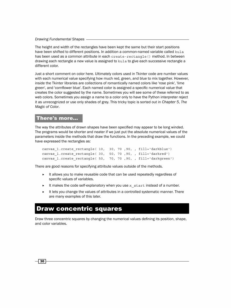
The height and width of the rectangles have been kept the same but their start positions have been shifted to different positions. In addition a common-named variable called kula has been used as a common attribute in each create-rectangle() method. In between drawing each rectangle a new value is assigned to kula to give each successive rectangle a different color.
Just a short comment on color here. Ultimately colors used in Tkinter code are number values with each numerical value specifying how much red, green, and blue to mix together. However, inside the Tkinter libraries are collections of romantically named colors like 'rose pink', 'lime green', and 'cornflower blue'. Each named color is assigned a specific numerical value that creates the color suggested by the name. Sometimes you will see some of these referred to as web colors. Sometimes you assign a name to a color only to have the Python interpreter reject it as unrecognized or use only shades of grey. This tricky topic is sorted out in Chapter 5, The Magic of Color.
There's more...The way the attributes of drawn shapes have been specified may appear to be long winded. The programs would be shorter and neater if we just put the absolute numerical values of the parameters inside the methods that draw the functions. In the preceding example, we could have expressed the rectangles as:
canvas_1.create_rectangle( 10, 30, 70 ,90, , fill='darkblue')canvas_1.create_rectangle( 30, 50, 70 ,90, , fill='darkred')canvas_1.create_rectangle( 50, 70, 70 ,90, , fill='darkgreen')
There are good reasons for specifying attribute values outside of the methods.
It allows you to make reusable code that can be used repeatedly regardless of specific values of variables.
It makes the code self-explanatory when you use x_start instead of a number.
It lets you change the values of attributes in a controlled systematic manner. There are many examples of this later.
Draw concentric squaresDraw three concentric squares by changing the numerical values defining its position, shape, and color variables.

Chapter 2
31
How to do it...The instructions used in recipe 1 should be used.
Just use the name 3concentric_squares.py when you write, save, and execute this program.
# 3concentric_squares.py#>>>>>>>>>>>>>>>>>from Tkinter import *root = Tk()root.title('Concentric squares')
cw = 200 # canvas widthch = 400 # canvas heightcanvas_1 = Canvas(root, width=cw, height=200, background="green")canvas_1.grid(row=0, column=1)
# dark bluex_center= 100y_center= 100x_width= 100y_height= 100kula= "darkblue"canvas_1.create_rectangle( x_center - x_width/2, \ y_center - y_height/2,\ x_center + x_width/2, y_center + y_height/2, fill=kula)
#dark redx_width= 80y_height= 80kula ="darkred"canvas_1.create_rectangle( x_center - x_width/2, \ y_center - y_height/2,\ x_center + x_width/2, y_center + y_height/2, fill=kula)
#dark greenx_width= 60y_height= 60kula ="darkgreen"canvas_1.create_rectangle( x_center - x_width/2, \ y_center - y_height/2,\ x_center + x_width/2, y_center + y_height/2, fill=kula)root.mainloop()#>>>>>>>>>>>>>>>>>>>>>>>>>>>>>>>>>>>>>>>>>>>

Drawing Fundamental Shapes
32
How it works...The results are given in the next screenshot.
In this recipe, we have specified where we want the geometric center of the rectangles located. This is at the position [x_center, y_center] in each instance. You need to do this whenever you want to draw shapes that are concentric. Generally it is always awkward to try and position the center of some drawn figure by manipulating the bottom-right corner. It does of course mean that there is a small amount of arithmetic in calculating where the bottom-left and top-right corners of the bounding box are but this is a small price to pay for the artistic freedom you gain. You only have to use this technique once and it is at your beck and call forever.
A circle from an ovalThe best way to draw a circle is to use the Tkinter's create_oval() method from the canvas widget.
How to do it...The instructions used in the first recipe should be used.
Just use the name circle_1.py when you write, save, and execute this program.
#circle_1.py#>>>>>>>>>>>>>>from Tkinter import *root = Tk()root.title('A circle')
cw = 150 # canvas widthch = 140 # canvas height

Chapter 2
33
canvas_1 = Canvas(root, width=cw, height=ch, background="white")canvas_1.grid(row=0, column=1)
# specify bottom-left and top-right as a set of four numbers named # 'xy'xy = 20, 20, 120, 120
canvas_1.create_oval(xy)root.mainloop()
How it works...The results are given in the next screenshot, showing a basic circle.
A circle is just an ellipse whose height and width are equal. In the example here, we have created a circle with the a very compact-looking statement: canvas_1.create_oval(xy).
The compactness comes from the trick of specifying the dimension attributes as a Python tuple xy = 20, 20, 420, 420 . It actually would be better in other instances to use a list such as xy = [ 20, 20, 420, 420 ] because a list allows you to alter the value of the individual member variables, whereas a tuple is an unchangeable sequence of constant values. Tuples are referred to as immutable.
There's more...Drawing a circle as a special case of an oval is definitely the best way to draw circles. An inexperienced user of Tkinter may be tempted into using an arc to do the job. This is a mistake because as shown in the next recipe the behavior of the create_arc() method does not allow an unblemished circle to be drawn.

Drawing Fundamental Shapes
34
A circle from an arcAnother way to make a circle is to use the create_arc() method. This method may appear to be a more natural way to make circles but it does not allow you to quite complete the circle. If you do try to the circle disappears.
How to do it...The instructions used in the first example should be used.
Just use the name arc_circle.py when you write, save and execute this program.
# arc_circle.py#>>>>>>>>>>>>>>>>>>>>>>>>>>>>>>>>>>>>> from Tkinter import *root = Tk()root.title('Should be a circle')cw = 210 # canvas widthch = 130 # canvas heightcanvas_1 = Canvas(root, width=cw, height=ch, background="white")canvas_1.grid(row=0, column=1)
xy = 20, 20, 320, 320 # bounding box from x0,y0 to x1, y1 # The Arc is drawn from start_angle, in degrees to finish_angle.# but if you try to complete the circle at 360 degrees it evaporates.canvas_1.create_arc(xy, start=0, extent=359.999999999, fill="cyan")root.mainloop()#>>>>>>>>>>>>>>>>>>>>>>>>>>>>>>>>>>>>>>
How it works...The results are given in the next screenshot, showing a failed circle resulting from create_arc().

Chapter 2
35
Generally the create_arc() method is not the best method of making complete circles because an attempt to go from 0 to 360 degrees results in the disappearance of the circle from view. Rather use the create_oval() method. However, there are occasions when you need the properties of the create_arc() method to be able to create a particular distribution of color. See the color wheel in the later chapters for a good example of this.
There's more...The create_arc() method is well suited to the production of the pie charts favored in corporate presentations. The create_arc() method draws a segment of a circle with the ends of the arc joined to the center by radial lines. But if we just want to draw a circle those radial lines are unwanted.
Three arc ellipsesThree elliptic arcs are drawn.
How to do it...The instructions used in recipe 1 should be used.
Just use the name 3arc_ellipses.py when you write, save, and execute this program.
# 3arc_ellipses.py#>>>>>>>>>>>>>>>>>>>>>>>>>>>>>>>>>>>>>>>>> from Tkinter import *root = Tk()root.title('3arc ellipses')
cw = 180 # canvas widthch = 180 # canvas heightcanvas_1 = Canvas(root, width=cw, height=ch)canvas_1.grid(row=0, column=1)
xy_1 = 20, 80, 80, 20xy_2 = 20, 130, 80, 100xy_3 = 100, 130, 140, 20
canvas_1.create_arc(xy_1, start=20, extent=270, fill="red")canvas_1.create_arc(xy_2, start=-50, extent=290, fill="cyan")canvas_1.create_arc(xy_3, start=150, extent=-290, fill="blue")root.mainloop()#>>>>>>>>>>>>>>>>>>>>>>>>>>>>>>>>>>>>>>>>>>>

Drawing Fundamental Shapes
36
How it works...The results are given in the next screenshot, showing well-behaved create_arc() ellipses.
The point to note here is that just like rectangles and ovals; the overall shape of the drawn object is governed by the shape of the bounding box. Start and finish (that is extent) angles are expressed in conventional degrees. Note that if trigonometry functions are going to be used then the circular measure has to be radians and not degrees.
There's more...The create_arc() method has been made user-friendly by requiring angular measurements in degrees rather than radians because most people can visualize degree amounts more easily than radians. But you need to know this is NOT the case with angular measurement in any function used by the math module. All the trigonometric functions like sine, cosine, and tangent use radian angular measurement which are only a minor convenience. The math module provides easy to use conversion functions.
PolygonsDraw a polygon. A polygon is a closed, multi-sided figure. These sides are made up of straight line segments. The specification of points is identical to that of multi-segment lines.
How to do it...The instructions used in recipe 1 should be used.
Just use the name triangle_polygon.py when you write, save, and execute this program.
# triangle_polygon.py#>>>>>>>>>>>>>>>> from Tkinter import *root = Tk()

Chapter 2
3�
root.title('triangle')
cw = 160 # canvas widthch = 80 # canvas heightcanvas_1 = Canvas(root, width=cw, height=ch, background="white")canvas_1.grid(row=0, column=1)
# point 1 point 2 point 3canvas_1.create_polygon(140,30, 130,70, 10,50, fill="red")root.mainloop()
How it works...The results are given in the next screenshot, showing a polygon triangle.
The create_polygon() method draws a sequence of straight line segments between the points specified as the arguments of the method. The final point is automatically joined to the first point to close the figure. As the figure is closed you can fill the interior with color.
A star polygonDraw a five-pointed star using named variables to specify the polygon attributes so that all the points or vertexes or tips of the star are defined with reference to a single start position. We refer to this position as the anchor position.
How to do it...The instructions used in recipe 1 should be used.
Just use the name star_polygon.py when you write, save, and execute this program.
# star_polygon.py#>>>>>>>>>>>> from Tkinter import *root = Tk()root.title(Polygon')

Drawing Fundamental Shapes
3�
cw = 140 # canvas widthch = 80 # canvas heightcanvas_1 = Canvas(root, width=cw, height=ch, background="white")canvas_1.grid(row=0, column=1)
# blue star, anchored to an anchor point.x_anchor = 15y_anchor = 50
canvas_1.create_polygon(x_anchor, y_anchor,\ x_anchor + 20, y_anchor - 40,\ x_anchor + 30, y_anchor + 10,\ x_anchor, y_anchor - 30,\ x_anchor + 40, y_anchor - 20,\ fill="blue")root.mainloop() #>>>>>>>>>>>>>>>>>>>>>>>>>>>>>>>>>>>>>>>>>
How it works...The results are given in the next screenshot, a polygon star.
The first position of the star is the point [x_anchor, y_anchor]. All the other points are positive or negative additions to the position of the anchor point. This concept was introduced in the recipes for the three superimposed rectangles. This idea of drawing complicated shapes with reference to a point defined as a pair of named variables is very useful and is used extensively in the second half of this book.
To improve code readability, the pairs of x and y variables defining each point are laid out vertically making use of the line continuation character \ (backslash).

Chapter 2
3�
Cloning and resizing starsA technique of simultaneous re-positioning and resizing a set of stars is shown.
How to do it...The instructions used in recipe 1 should be used.
Just use the name clone_stars.py when you write, save, and execute this program.
# clone_stars.py#>>>>>>>>>>>>>>>>>>>>>>>>>>>>>>>>>>>>>>>from Tkinter import *root = Tk()root.title('Re-sized and re-positioned polygon stars')
cw = 200 # canvas widthch = 100 # canvas heightcanvas_1 = Canvas(root, width=cw, height=ch, background="white")canvas_1.grid(row=0, column=1)
# blue star, anchored to an anchor point.x_anchor = 15y_anchor = 150size_scaling = 1
canvas_1.create_polygon(x_anchor, y_anchor,\ x_anchor + 20 * size_scaling, y_anchor - \ 40* size_scaling,\ x_anchor + 30 * size_scaling, y_anchor + \ 10* size_scaling,\ x_anchor, y_anchor - 30* size_scaling,\ x_anchor + 40 * size_scaling, y_anchor - \ 20* size_scaling,\ fill="green") size_scaling = 2x_anchor = 80y_anchor = 120canvas_1.create_polygon(x_anchor, y_anchor,\ x_anchor + 20 * size_scaling, y_anchor - \ 40* size_scaling,\ x_anchor + 30 * size_scaling, y_anchor + \ 10* size_scaling,\
Dow
nlo
ad fro
m W
ow
! eBook
<w
ww
.wow
ebook.
com
>
Drawing Fundamental Shapes
40
x_anchor, y_anchor - 30* size_scaling,\ x_anchor + 40 * size_scaling, y_anchor - \ 20* size_scaling,\ fill="darkgreen") size_scaling = 3x_anchor = 160y_anchor = 110canvas_1.create_polygon(x_anchor, y_anchor,\ x_anchor + 20 * size_scaling, y_anchor - \ 40* size_scaling,\ x_anchor + 30 * size_scaling, y_anchor + \ 10* size_scaling,\ x_anchor, y_anchor - 30* size_scaling,\ x_anchor + 40 * size_scaling, y_anchor - \ 20* size_scaling,\ fill="lightgreen") size_scaling = 3x_anchor = 160y_anchor = 110canvas_1.create_polygon(x_anchor, y_anchor,\ x_anchor + 20 * size_scaling, y_anchor - \ 40* size_scaling,\ x_anchor + 30 * size_scaling, y_anchor + \ 10* size_scaling,\ x_anchor, y_anchor - 30* size_scaling,\ x_anchor + 40 * size_scaling, y_anchor - \ 20* size_scaling,\ fill="forestgreen")root.mainloop()#>>>>>>>>>>>>>>>>>>>>>>>>>>>>>>>>>>>>>>>
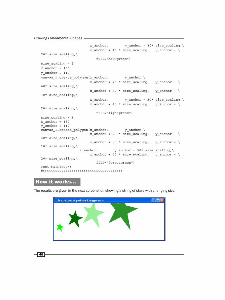
How it works...The results are given in the next screenshot, showing a string of stars with changing size.

Chapter 2
41
In addition to the variable and conveniently re-assigned anchor point of the polygon star we have now introduced an amplification factor that can change the size of any particular star without distorting it.
There's more...The last three examples have illustrated some important and fundamental ideas used to draw pre-defined shapes in any size and in any position. It was important to separate these effects in different examples at this stage so that the separate actions are easy to understand. Later on, where the effects are used in combination, it becomes difficult to wrap your head around what is happening, particularly if extra transformations like rotation are involved. If we animate code that generates images it can be much easier to understand geometric relationships. By animate, I mean the display of successive images separated by short-time intervals similar to the way images in movies are manipulated. Such time-regulated animation, surprisingly, offers methods of examining the behavior of image-generating code in a way that is much more intuitive and clear to the human brain. This idea is developed in the later chapters.


3Handling Text
In this chapter, we will cover:
Simple text
Text font type, size, and color
Placement of text – north, south, east, and west
Placement of text – right and left justification
Fonts available on your platform
IntroductionText can be tricky. We need to be able to manipulate font family, size, color, and placement. Placement in turn requires that we specify where text must begin and what areas it should be confined to.
In this chapter, we focus on handling text on a canvas.
Simple textThis is how to place text onto your canvas.
How to do it...1. In a text editor, type the code given in the following code.
2. Save this as a file named text_1.py, inside the directory called constr again.
3. As before, open up an X terminal or DOS window if you are using MS Windows.
4. Change directory into constr - where text_1.py is located.

Handling Text
44
5. Type text_1.py and your program should execute.
# text_1.py#>>>>>>>>>>from Tkinter import *root = Tk()root.title('Basic text')cw = 400 # canvas widthch = 50 # canvas heightcanvas_1 = Canvas(root, width=cw, height=ch, background="white")canvas_1.grid(row=0, column=1)
xy = 150, 20canvas_1.create_text(xy, text=" The default text size looks \ about 10.5 point")root.mainloop()
How it works...The results are given in the following screenshot:
Placing text exactly where you want it on a screen can be tricky because of the way font height and inter-character spacing as well as the text window dimensions all interfere with each other. You will probably have to spend a bit of time experimenting to get your text as you want it.
There's more...Text placed onto a canvas offers a useful alternative to the often used print function as a debugging tool. You can send the values of many variables for display onto a canvas and watch their values change.
As will be demonstrated in the chapter on animation, the easiest way of observing the interaction of complex numerical relationships is to animate them in some way.

Chapter 3
45
Text font type, size, and colorIn a very similar manner to the way attributes are specified for lines and shapes, font type, size, and color are governed by the attributes of the create_text() method.
Getting readyNothing needed here.
How to do it...The instructions used in recipe 1 should be used.
Just use the name 4color_text.py when you write, save, and execute this program.
# 4color_text.py#>>>>>>>>>>>>>>from Tkinter import *root = Tk() root.title('Four color text')
cw = 500 # canvas widthch = 140 # canvas heightcanvas_1 = Canvas(root, width=cw, height=ch, background="white")canvas_1.grid(row=0, column=1)
xy = 200, 20 canvas_1.create_text(200, 20, text=" text normal SansSerif 20", \ fill='red',\ width=500, font='SansSerif 20 ')canvas_1.create_text(200, 50, text=" text normal Arial 20", \ fill='blue',\ width=500, font='Arial 20 ')canvas_1.create_text(200, 80, text=" text bold Courier 20", \ fill='green',\ width=500, font='Courier 20 bold')canvas_1.create_text(200, 110, text=" bold italic BookAntiqua 20",\ fill='violet', width=500, font='Bookantiqua 20 bold')root.mainloop()#>>>>>>>>>>>>>>>>>>>>>>>>>>>>>>>>>>>>
Handling Text
46
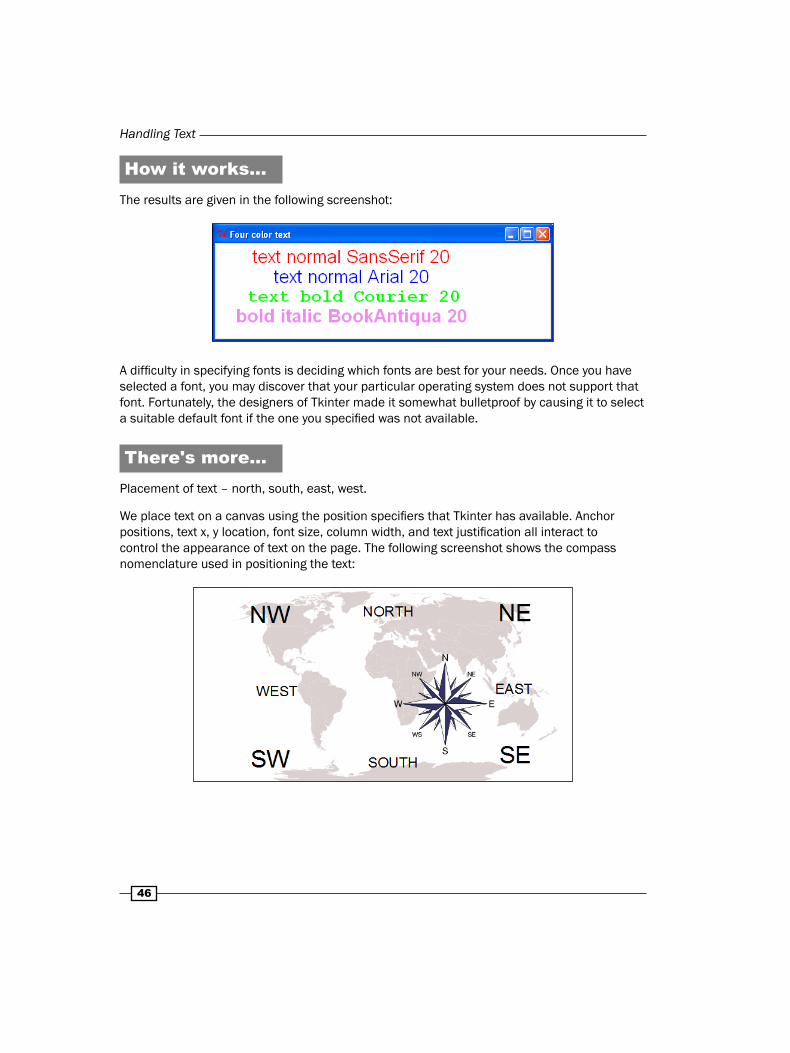
How it works...The results are given in the following screenshot:
A difficulty in specifying fonts is deciding which fonts are best for your needs. Once you have selected a font, you may discover that your particular operating system does not support that font. Fortunately, the designers of Tkinter made it somewhat bulletproof by causing it to select a suitable default font if the one you specified was not available.
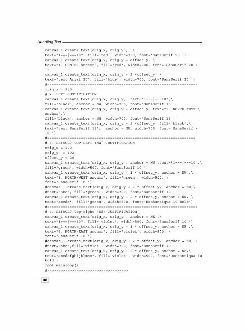
There's more...Placement of text – north, south, east, west.
We place text on a canvas using the position specifiers that Tkinter has available. Anchor positions, text x, y location, font size, column width, and text justification all interact to control the appearance of text on the page. The following screenshot shows the compass nomenclature used in positioning the text:

Chapter 3
4�
Getting readyPlacing text onto a canvas is tricky until we understand the navigation system that Tkinter uses. Here is how it works. All text goes into an invisible box. The box is like an empty picture frame placed over a nail on a board. The Tkinter canvas is the board and the empty frame is the box that the text we type is going to fit inside. The nail is the x and y location. The empty frame can be moved so that the nail is in the top left-corner (North-West) or the bottom right (South-East) or in the center or the other corners or sides. The following screenshot shows the imaginary frame on the canvas that contains the text:
How to do it...Execute the code and observe how the various text position specifiers
control the appearance of the text.
# anchor_align_text_1.py#>>>>>>>>>>>>>>>>>>>>>>>>>>>>>>>>>>>>>from Tkinter import *root = Tk()root.title('Anchoring Text North, South, East, West')cw = 650 # canvas widthch = 180 # canvas heightcanvas_1 = Canvas(root, width=cw, height=ch, background="white")canvas_1.grid(row=0, column=1)
orig_x = 220orig_y = 20 offset_y = 30 # 1. DEFAULT CENTER JUSTIFICATION# width is maximum line length.
Handling Text
4�
canvas_1.create_text(orig_x, orig_y , \text="1===|===10", fill='red', width=700, font='SansSerif 20 ')canvas_1.create_text(orig_x, orig_y + offset_y, \text="1. CENTER anchor", fill='red', width=700, font='SansSerif 20 \ ') canvas_1.create_text(orig_x, orig_y + 2 *offset_y, \text="text Arial 20", fill='blue', width=700, font='SansSerif 20 ')#===================================================================orig_x = 380# 2. LEFT JUSTIFICATION canvas_1.create_text(orig_x, orig_y, text="1===|===10",\fill='black', anchor = NW, width=700, font='SansSerif 16 ')canvas_1.create_text(orig_x, orig_y + offset_y, text="2. NORTH-WEST \ anchor",\fill='black', anchor = NW, width=700, font='SansSerif 16 ') canvas_1.create_text(orig_x, orig_y + 2 *offset_y, fill='black',\text="text SansSerif 16", anchor = NW, width=700, font='SansSerif \ 16 ')#==================================================================# 3. DEFAULT TOP-LEFT (NW) JUSTIFICATIONorig_x = 170orig_y = 102offset_y = 20canvas_1.create_text(orig_x, orig_y , anchor = NW ,text="1===|===10",\fill='green', width=500, font='SansSerif 10 ')canvas_1.create_text(orig_x, orig_y + 1 * offset_y, anchor = NW ,\text="3. NORTH-WEST anchor", fill='green', width=500, \ font='SansSerif 10 ')#canvas_1.create_text(orig_x, orig_y + 2 * offset_y, anchor = NW,\#text="abc", fill='green', width=700, font='SansSerif 10 ')canvas_1.create_text(orig_x, orig_y + 2 * offset_y, anchor = NW, \text="abcde", fill='green', width=500, font='Bookantiqua 10 bold')#===================================================================# 4. DEFAULT Top-right (SE) JUSTIFICATIONcanvas_1.create_text(orig_x, orig_y , anchor = NE ,\text="1===|===10", fill='violet', width=500, font='SansSerif 10 ')canvas_1.create_text(orig_x, orig_y + 1 * offset_y, anchor = NE ,\text="4. NORTH-EAST anchor", fill='violet', width=500, \ font='SansSerif 10 ')#canvas_1.create_text(orig_x, orig_y + 2 * offset_y, anchor = NE, \#text="abc",fill='violet', width=700, font='SansSerif 10 ')canvas_1.create_text(orig_x, orig_y + 2 * offset_y, anchor = NE,\text="abcdefghijklmno", fill='violet', width=500, font='Bookantiqua 10 bold')root.mainloop()#>>>>>>>>>>>>>>>>>>>>>>>>>>>>>>>>>>>>

Chapter 3
4�
How it works...The results are given in the following screenshot:
Alignment of text – left and right justifyWe now concentrate particularly on how the justification of the text in columns interacts with column anchor positions.
Getting readyThe following code contains a paragraph that is much too long to fit onto a single line. This is where we see how the term justify lets us decide whether we want the text to line up to the right of the column or to its left or perhaps even the center. The column width, in pixels, is specified and then the text is made to fit.
How to do it...Run the following code and observe that the height of the column is only confined by the height of the canvas but the width, anchor position, justification, and font size determine how the text gets laid out on the canvas.
# justify_align_text_1.py#>>>>>>>>>>>>>>>>>>>>>>>>>>>>>>>>>>>>>from Tkinter import *root = Tk()root.title('North-south-east-west Placement with LEFT and RIGHT \ justification of Text')
cw = 850 # canvas widthch = 720 # canvas height

Handling Text
50
canvas_1 = Canvas(root, width=cw, height=ch, background="white")canvas_1.grid(row=0, column=1)
orig_x = 220orig_y = 20 offset_y = 20 jolly_text = "And now ladies and gentlemen she will attempt - for the very first time in the history of 17 Shoeslace street - a one handed right arm full toss teacup fling. Yes you lucky listners you are about to witness what, in recorded history, has never been attempted before without the aid of hair curlers and fluffy slippers."# width is maximum line length.#=================================================================# 1. Top-left (NE) ANCHOR POINT, no column justification specified.canvas_1.create_text(orig_x, orig_y + 1 * offset_y, anchor = NE \ ,text="1. \NORTH-EAST anchor, no column justification", fill='blue', width=200, \ font='Arial 10')canvas_1.create_text(orig_x, orig_y + 3 * offset_y, anchor = NE, \ text=jolly_text,\ fill='blue', width=150, font='Arial 10')#==================================================================# 2. Top-right (NW) ANCHOR POINT, no column justification specified.canvas_1.create_text(orig_x, orig_y + 1 * offset_y, anchor = NW \ ,text="2. \NORTH-WEST ancho, no column justification", fill='red', width=200, \ font='Arial 10')canvas_1.create_text(orig_x, orig_y + 3 * offset_y, anchor = NW, \ text= jolly_text,\ fill='red', width=200, font='Arial 10')#==================================================================orig_x = 600canvas_1.create_text(orig_x, orig_y + 1 * offset_y, anchor = NE \ ,text="3. \SOUTH-EAST anchor, no column justification",fill='black', width=200, \ font='Arial 10')canvas_1.create_text(orig_x, orig_y + 1 * offset_y, anchor = NW \ ,text="4. \SOUTH-WEST anchor, no column justification", fill='#666666', \ width=200, font='Arial 10')#============================================================orig_x = 600orig_y = 280 # 3. BOTTOM-LEFT (SW) JUSTIFICATION, no column justification # specified.

Chapter 3
51
canvas_1.create_text(orig_x, orig_y + 2 * offset_y, anchor = SW, \ text=jolly_text,\ fill='#666666', width=200, font='Arial \ 10')#==================================================================# 4. TOP-RIGHT (SE) ANCHOR POINT, no column justification specified.canvas_1.create_text(orig_x, orig_y + 2 * offset_y, anchor = SE, \ text=jolly_text,\ fill='black', width=150, font='Arial 10')#===================================================================orig_y = 350orig_x = 200 # 5. Top-right (NE) ANCHOR POINT, RIGHT column justification # specified.canvas_1.create_text(orig_x, orig_y + 1 * offset_y, anchor = NE , \ justify=RIGHT,\text="5. NORTH-EAST anchor, justify=RIGHT", fill='blue', width=200, \ font='Arial 10 ')canvas_1.create_text(orig_x, orig_y + 3 * offset_y, anchor = NE, \ justify=RIGHT, \text=jolly_text, fill='blue', width=150, font='Arial 10')#===================================================================# 6. TOP-LEFT (NW) ANCHOR POINT, RIGHT column justification specified.canvas_1.create_text(orig_x, orig_y + 1 * offset_y, anchor = NW \ ,text="6.\NORTH-WEST anchor, justify=RIGHT", fill='red', width=200, \ font='Arial 10 ')canvas_1.create_text(orig_x, orig_y + 3 * offset_y, anchor = NW, \ justify=RIGHT,\text=jolly_text, fill='red', width=200, font='Arial 10')
#===================================================================orig_x = 600# Header lines for 7. and 8.canvas_1.create_text(orig_x, orig_y + 1 * offset_y, anchor = NE \ ,text="7. \SOUTH-EAST anchor, justify= CENTER", fill='black', width=160, \ font='Arial 10 ')canvas_1.create_text(orig_x, orig_y + 1 * offset_y, anchor = NW , \ text="8.\SOUTH-WEST anchor, justify= CENTER", fill='#666666', width=200, \ font='Arial 10 ')#==================================================================orig_y = 600# 7. TOP-RIGHT (SE) ANCHOR POINT, CENTER column justification # specified.
Dow
nlo
ad fro
m W
ow
! eBook
<w
ww
.wow
ebook.
com
>

Handling Text
52
canvas_1.create_text(orig_x, orig_y + 4 * offset_y, anchor = SE, \ justify= CENTER,\text=jolly_text, fill='black', width=150, font='Arial 10')#=================================================================== # 8. BOTTOM-LEFT (SW) ANCHOR POINT, CENTER column justification # specified.canvas_1.create_text(orig_x, orig_y + 4 * offset_y, anchor = SW, \ justify= CENTER,\text=jolly_text, fill='#666666', width=200, font='Arial 10')
root.mainloop()#>>>>>>>>>>>>>>>>>>>>>>>>>>>>>>>>>>>>
How it works...The interaction of column width, anchor position, and justification are complex and the clearest way to explain the results is with annotated pictures of the canvas display resulting from execution. The following screenshot shows Top-right (NE) ANCHOR POINT, no justification specified (default LEFT justification).

Chapter 3
53
The following screenshot shows the Top-right(SE)ANCHOR POINT, no justification specified:
The following screenshot shows the Bottom-right (SE) ANCHOR POINT, CENTER justification specified:
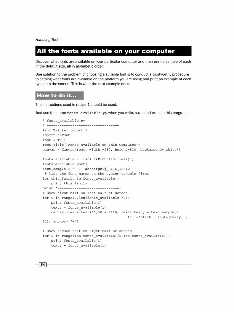
Handling Text
54
All the fonts available on your computerDiscover what fonts are available on your particular computer and then print a sample of each in the default size, all in alphabetic order.
One solution to the problem of choosing a suitable font is to conduct a trustworthy procedure to catalog what fonts are available on the platform you are using and print an example of each type onto the screen. This is what the next example does.
How to do it...The instructions used in recipe 1 should be used.
Just use the name fonts_available.py when you write, save, and execute this program.
# fonts_available.py# ==================================from Tkinter import *import tkFontroot = Tk()root.title('Fonts available on this Computer')canvas = Canvas(root, width =930, height=830, background='white')
fonts_available = list( tkFont.families() )fonts_available.sort()text_sample = ' : abcdefghij_HIJK_12340' # list the font names on the system console first.for this_family in fonts_available : print this_familyprint '============================='# Show first half on left half of screen .for i in range(0,len(fonts_available)/2): print fonts_available[i] texty = fonts_available[i] canvas.create_text(50,30 + i*20, text= texty + text_sample,\ fill='black', font=(texty, \ 12), anchor= "w")
# Show second half on right half of screen .for i in range(len(fonts_available)/2,len(fonts_available)): print fonts_available[i] texty = fonts_available[i]

Chapter 3
55
canvas.create_text(500,30 + (i-len(fonts_available)/2 )*20, \ text= texty+ text_sample, fill='black', \ font=(texty, 12),anchor= "w")
canvas.pack()root.mainloop()
How it works...The results are given in the following screenshot showing all fonts available to Python on a specific operating system.
This program is very useful when you want to select pleasing and suitable fonts. Fonts available can vary significantly from platform to platform. So here we make use of the families() method belonging to the tkFont module to put the names of the font families into a list named fonts_available. The list is sorted into alphabetic order using fonts_available.sort().

Handling Text
56
Finally, two handy things have been used.
Firstly, the list of fonts has been made neat by anchoring the text to the west or left side by use of the anchor= "w" attribute of the create_text method.
Secondly, it is the very useful len() function in len(fonts_available).
This function gives back to you ("returns" in programming parlance) the number of items in a list. It is very handy when defining how many times a for loop iteration should go on for when you have no idea what that number is going to be. In this example we need to write the name of a font and a text sample for each font name in a list that has not yet been discovered when we write the code.
4Animation Principles
In this chapter, we will cover:
Static shifting of a ball
Timed shifting of a ball
Animation – timed draw-and-erase cycles
Two balls moving unimpeded
A ball that bounces
Bouncing in a gravitational field
Colliding balls with tracer trails
Elastic ball against ball collisions
Dynamic debugging
Trajectory tracing
Rotating a line and vital trigonometry
Rotating lines which rotate lines
A digital flower
IntroductionAnimation is about making graphic objects move smoothly around a screen. The method to create the sensation of smooth dynamic action is simple:
1. First present a picture to the viewer's eye.
2. Allow the image to stay in view for about one-twentieth of a second.
3. With a minimum of delay, present another picture where objects have been shifted by a small amount and repeat the process.

Animation Principles
5�
Besides the obvious applications of making animated figures move around on a screen for entertainment, animating the results of computer code gives you powerful insights into how code works at a detailed level. Animation offers an extra dimension to the programmers' debugging arsenal. It provides you with an all encompassing, holistic view of software execution in progress that nothing else can.
Static shifting of a ballWe make an image of a small colored disk and draw it in a sequence of different positions.
How to do it...
Execute the program shown in exactly the same way as all the examples in Chapter 2, Drawing Fundamental Shapes and you will see a neat row of colored disks laid on top of each other going from top left to bottom right. The idea is to demonstrate the method of systematic position shifting that we will use again and again throughout the book.
# moveball_1.py#>>>>>>>>>>>>>from Tkinter import *root = Tk()root.title("shifted sequence")cw = 250 # canvas widthch = 130 # canvas height chart_1 = Canvas(root, width=cw, height=ch, background="white")chart_1.grid(row=0, column=0)# The parameters determining the dimensions of the ball and its # position.# ==========================================posn_x = 1 # x position of box containing the ball (bottom)posn_y = 1 # y position of box containing the ball (left edge)shift_x = 3 # amount of x-movement each cycle of the 'for' loopshift_y = 2 # amount of y-movement each cycle of the 'for' loopball_width = 12 # size of ball - width (x-dimension)ball_height = 12 # size of ball - height (y-dimension)color = "violet" # color of the ball
for i in range(1,50): # end the program after 50 position shifts posn_x += shift_x posn_y += shift_y
Chapter 4
5�
chart_1.create_oval(posn_x, posn_y, posn_x + ball_width,\ posn_y + ball_height, fill=color)
root.mainloop()#>>>>>>>>>>>>>>>>>>>>>>>>>>>>>>>>>>>>>>>>>>
How it works...A simple ball is drawn on a canvas in a sequence of steps, one on top of the other. For each step, the position of the ball is shifted by three pixels as specified by the size of shift_x. Similarly, a downward shift of two pixels is applied by an amount to the value of shift_y. shift_x and shift_y only specify the amount of shift, but they do not make it happen. What makes it happen are the two commands posn_x += shift_x and posn_y += shift_y. posn is the abbreviation for position. An important word of explanation of this notation is needed here because we use it often throughout the book. It is neat and handy.
posn_x += shift_x means "take the variable posn_x and add to it an amount shift_x." It is the same as posn_x = posn_x + shift_x.
Another minor point to note is the use of the line continuation character, the backslash "\". We use this when we want to continue the same Python command onto a following line to make reading easier. Strictly speaking for text inside brackets "(...)" this is not needed. In this particular case you can just insert a carriage return character. However, the backslash makes it clear to anyone reading your code what your intention is.
There's more...The series of ball images in this recipe were drawn in a few microseconds. To create decent looking animation, we need to be able to slow the code execution down by just the right amount. We need to draw the equivalent of a movie frame onto the screen and keep it there for a measured time and then move on to the next, slightly shifted, image. This is done in the next recipe.
Time-controlled shifting of a ballHere we introduce the time control function canvas.after(milliseconds) and the canvas.update() function that refreshes the image on the canvas. These are the cornerstones of animation in Python.
Control of when code gets executed is made possible by the time module that comes with the standard Python library.

Animation Principles
60
How to do it...Execute the program as previously. What you will see is a diagonal row of disks being laid in a line with a short delay of one fifth of a second (200 milliseconds) between updates. The result is shown in the following screenshot showing the ball shifting in regular intervals.
# timed_moveball_1.py#>>>>>>>>>>>>>>>>>>>>>>>>>>>>>>>>>>>>>>>>>>>>from Tkinter import *root = Tk()root.title("Time delayed ball drawing")
cw = 300 # canvas widthch = 130 # canvas height chart_1 = Canvas(root, width=cw, height=ch, background="white")chart_1.grid(row=0, column=0)
cycle_period = 200 # time between fresh positions of the ball # (milliseconds).# The parameters determining the dimensions of the ball and it's # position.posn_x = 1 # x position of box containing the ball (bottom).posn_y = 1 # y position of box containing the ball (left edge).shift_x = 3 # amount of x-movement each cycle of the 'for' loop.shift_y = 3 # amount of y-movement each cycle of the 'for' loop. ball_width = 12 # size of ball - width (x-dimension).ball_height = 12 # size of ball - height (y-dimension).color = "purple" # color of the ball
for i in range(1,50): # end the program after 50 position shifts. posn_x += shift_x posn_y += shift_y
chart_1.create_oval(posn_x, posn_y, posn_x + ball_width,\ posn_y + ball_height, fill=color)
Chapter 4
61
chart_1.update() # This refreshes the drawing on the canvas. chart_1.after(cycle_period) # This makes execution pause for 200 # milliseconds.
root.mainloop()
How it works...This recipe is the same as the previous one except for the canvas.after(...) and the canvas.update() methods. These are two functions that come from the Python library. The first gives you some control over code execution time by allowing you to specify delays in execution. The second forces the canvas to be completely redrawn with all the objects that should be there. There are more complicated ways of refreshing only portions of the screen, but they create difficulties so they will not be dealt with here.
The canvas.after(your-chosen-milliseconds) method simply causes a timed-pause to the execution of the code. In all the preceding code, the pause is executed as fast as the computer can do it, then when the pause, invoked by the canvas.after() method is encountered, execution simply gets suspended for the specified number of milliseconds. At the end of the pause, execution continues as if nothing ever happened.
The canvas.update() method forces everything on the canvas to be redrawn immediately rather than wait for some unspecified event to cause the canvas to be refreshed.
There's more...The next step in effective animation is to erase the previous image of the object being animated shortly before a fresh, shifted clone is drawn on the canvas. This happens in the next example.
The robustness of TkinterIt is also worth noting that Tkinter is robust. When you give position coordinates that are off the canvas, Python does not crash or freeze. It simply carries on drawing the object 'off-the-page'. The Tkinter canvas can be seen as just a tiny window into an almost unlimited universe of visual space. We only see objects when they move into the view of the camera which is the Tkinter canvas.
Animation Principles
62
Complete animation using draw-move-pause-erase cycles
This recipe gives you the whole animation procedure. All the actions necessary for the human brain to interpret images on the retina as moving objects are present in this example. The whole craft of animation and the million dollar movies based thereon is demonstrated here in its simplest and purest form.
How to do it...Execute this program as we have done before. Note that this time we have reduced the timed pause to 50 milliseconds which is 20 times per second. This is close to the standard 24 frames per second used in movies. However, without a graphics card this time becomes less accurate as shorter pauses are specified. In addition, the distance moved between position shifts of the ball has been reduced to one pixel.
# move_erase_cycle_1.py# >>>>>>>>>>>>>>>>>>>>>>>>>>>>>>>>>>>>>>>>>>>>>>from Tkinter import *root = Tk()root.title("move-and-erase")cw = 230 # canvas widthch = 130 # canvas height chart_1 = Canvas(root, width=cw, height=ch, background="white")chart_1.grid(row=0, column=0)cycle_period = 50 # time between new positions of the ball # (milliseconds). # The parameters determining the dimensions of the ball and its # position.posn_x = 1 # x position of box containing the ball (bottom).posn_y = 1 # y position of box containing the ball (left edge).shift_x = 1 # amount of x-movement each cycle of the 'for' loop.shift_y = 1 # amount of y-movement each cycle of the 'for' loop.ball_width = 12 # size of ball - width (x-dimension).ball_height = 12 # size of ball – height (y-dimension).color = "hot pink" # color of the ball
for i in range(1,500): # end the program after 500 position shifts. posn_x += shift_x posn_y += shift_y

Chapter 4
63
chart_1.create_oval(posn_x, posn_y, posn_x + ball_width,\ posn_y + ball_height, fill=color) chart_1.update() # This refreshes the drawing on the canvas. chart_1.after(cycle_period) # This makes execution pause for 200 # milliseconds. chart_1.delete(ALL) # This erases everything on the canvas.
root.mainloop()# >>>>>>>>>>>>>>>>>>>>>>>>>>>>>>>>>>>>>>>>>>>>>>
How it works...The new element in this self-contained animation is the canvas.delete(ALL) method that clears the entire canvas of everything that was drawn on it. It is possible to erase only specific objects on the screen through the use of identification tags. This is not needed now. Selective object deletion using tags will be used in the last three recipes of this chapter.
There's more...How accurate is the timing of the pause() method?.
With modern computers, pauses of five milliseconds are realistic but the animation becomes jerky as the pause times get shorter.
More than one moving objectWe want to be able to develop programs where more than one independent graphic object co-exists and interacts according to some rules. This is how most computer games work. Pilot training simulators and serious engineering design models are designed on the same principles. We start this process simply by working up to an application that ends up with two balls bouncing off the walls and each other under the influence of gravity and energy loss.
How to do it...The following code is very similar to that in the previous recipe, except that two similar objects are created. They are independent of each other and do not interact in any way.
# two_balls_moving_1.py# >>>>>>>>>>>>>>>>>>>>>>>>>>>>>>>>>>>>>>>>>>>>>>from Tkinter import *root = Tk()root.title("Two balls")cw = 200 # canvas width
Dow
nlo
ad fro
m W
ow
! eBook
<w
ww
.wow
ebook.
com
>

Animation Principles
64
ch = 130 # canvas height chart_1 = Canvas(root, width=cw, height=ch, background="white")chart_1.grid(row=0, column=0)cycle_period = 100 # time between new positions of the ball # (milliseconds). # The parameters defining ball no 1.posn_x_1 = 1 # x position of box containing the ball (bottom).posn_y_1 = 1 # y position of box containing the ball (left edge).shift_x_1 = 1 # amount of x-movement each cycle of the 'for' loop.shift_y_1 = 1 # amount of y-movement each cycle of the 'for' loop.ball_width_1 = 12 # size of ball - width (x-dimension).ball_height_1 = 12 # size of ball - height (y-dimension).color_1 = "blue" # color of ball #1
# The parameters defining ball no 2.posn_x_2 = 180 # x position of box containing the ball (bottom).posn_y_2 = 180 # x position of box containing the ball (left # edge).shift_x_2 = -2 # amount of x-movement each cycle of the 'for' # loop.shift_y_2 = -2 # amount of y-movement each cycle of the 'for' # loop.ball_width_2 = 8 # size of ball - width (x-dimension).ball_height_2 = 8 # size of ball - height (y-dimension).color_2 = "green" # color of ball #2.
for i in range(1,100): # end the program after 50 position shifts. posn_x_1 += shift_x_1 posn_y_1 += shift_y_1 posn_x_2 += shift_x_2 posn_y_2 += shift_y_2
chart_1.create_oval(posn_x_1, posn_y_1, posn_x_1 + ball_width_1,\ posn_y_1 + ball_height_1, fill=color_1) chart_1.create_oval(posn_x_2, posn_y_2, posn_x_2 + ball_width_2,\ posn_y_2 + ball_height_2, fill=color_2) chart_1.update() # This refreshes the drawing on the canvas. chart_1.after(cycle_period) # This makes execution pause for 100 # milliseconds. chart_1.delete(ALL) # This erases everything on the canvasroot.mainloop()# >>>>>>>>>>>>>>>>>>>>>>>>>>>>>>>>>>>>>>>>>>>>>>

Chapter 4
65
How it works...The main point to note is that these programs, and many others in this book, are divided into five parts:
1. Creating the environment where objects will exist.
2. Defining the individual objects and their attributes.
3. Defining the rules of engagement between objects.
4. Creating the objects.
5. Using a loop to simulate the march of time by changing properties such as position at rates that mimic real-time motion.
6. Controlling the environment inside which the objects exist.
The environment in most of our examples is the Tkinter canvas. The objects that are going to exist inside the canvas environment in this example are two colored balls. The rules of engagement are that they will not have any effect on each other at all and they will not be affected by the edges of the canvas. Another rule of engagement is how their positions will shift each time the for loop is executed.
Finally the environment is controlled by the time regulated canvas.update() and canvas.delete(ALL) methods.
There's more...The principle idea demonstrated in this recipe is that we can create more than one similar, but different objects exist and react independently. This gives rise to the idea of object-oriented programming.
Python offers more than one way to use the ideas of object-oriented programming. In this book, we use three ways of making objects: lists, dictionaries, and classes.
A ball that bouncesNow and in the next three examples, we add rules of engagement that are increasingly complex. The overall objective is to introduce behaviors and interactions into our artificial world to make it behave more like the real world. We use numbers, calculations, and graphical drawings to represent aspects of the real world as we know it.
The first new behavior is that our colored disks will bounce elastically off the walls of the container that is the Tkinter canvas.

Animation Principles
66
How to do it...The code has purposely been kept as similar as possible to the previous four examples so that we feel we are still in familiar territory as the world we create gets increasingly more complicated. If we did not do this, we would get lost and bewildered. The whole secret in successfully constructing complex computer programs is to build it up gradually and systematically piece-by-piece. It is not a planned journey along a well-mapped road but rather a strenuous exploration through uncharted jungle.
# bounce_ball.py#>>>>>>>>>>>>>>>>>>>>>>>>>>>>>>>>>>>>>>>>>>from Tkinter import *import timeroot = Tk()root.title("The bouncer")cw = 200 # canvas widthch = 120 # canvas height chart_1 = Canvas(root, width=cw, height=ch, background="white")chart_1.grid(row=0, column=0)cycle_period = 50 # time between new positions of the ball # (milliseconds).# The parameters determining the dimensions of the ball and its position.posn_x = 1 # x position of box containing the ball (bottom).posn_y = 1 # x position of box containing the ball (left edge).shift_x = 1 # amount of x-movement each cycle of the 'for' loop.shift_y = 1 # amount of y-movement each cycle of the 'for' loop.ball_width = 12 # size of ball - width (x-dimension).ball_height = 12 # size of ball - height (y-dimension).color = "firebrick" # color of the ball
# Here is a function that detects collisions with the walls of the # container# and then reverses the direction of movement if a collision is # detected.def detect_wall_collision():global posn_x, posn_y, shift_x, shift_y, cw, cy if posn_x > cw : # Collision with right-hand container wall.shift_x = -shift_x # reverse direction. if posn_x < 0 : # Collision with left-hand wall.shift_x = -shift_x

Chapter 4
6�
if posn_y > ch : # Collision with floor.shift_y = -shift_y if posn_y < 0 : # Collision with ceiling.shift_y = -shift_y
for i in range(1,1000): # end the program after1000 position shifts. posn_x += shift_x posn_y += shift_y chart_1.create_oval(posn_x, posn_y, posn_x + ball_width,\ posn_y + ball_height, fill=color) detect_wall_collision() # Has the ball collided with # any container wall? chart_1.update() # This refreshes the drawing on the canvas. chart_1.after(cycle_period) # This makes execution pause # for 200 milliseconds. chart_1.delete(ALL) # This erases everything on the canvas.
root.mainloop()#>>>>>>>>>>>>>>>>>>>>>>>>>>>>>>>>>
How it works...The new feature here is the function detect_Wall_Collision(). Whenever it is called, it checks whether the position of the ball has moved outside the boundary of the canvas. If it has, the direction of the ball is reversed. This method is crude because it does not compensate for the size of the ball. Consequently the ball pops out of existence.
Bouncing in a gravity fieldIn this recipe, the influence of a gravitational field is added to the previous rule of bouncing off the canvas wall.
How to do it...What makes this recipe different to all the previous ones is a new attribute of the ball named velocity_y. With every cycle of the for i in range(0,300) loop the velocity is modified just as it would be in the gravitational field of our real world.
# gravityball.py# >>>>>>>>>>>>>>>>>>>>>>>>>>>>>from Tkinter import *root = Tk()root.title("Gravity bounce")

Animation Principles
6�
cw = 220 # canvas widthch = 200 # canvas heightGRAVITY = 4 chart_1 = Canvas(root, width=cw, height=ch, background="white")chart_1.grid(row=0, column=0)cycle_period = 30
# The parameters determining the dimensions of the ball and its # position.posn_x = 15 posn_y = 180 shift_x = 1 velocity_y = 50 ball_width = 12 ball_height = 12 color = "blue"
# The function that detects collisions with the walls and reverses # directiondef detect_wall_collision(): global posn_x, posn_y, shift_x, velocity_y, cw, cy if posn_x > cw -ball_width: # Collision with right-hand # container wall. shift_x = -shift_x # reverse direction. if posn_x < ball_width: # Collision with left-hand wall. shift_x = -shift_x if posn_y < ball_height : # Collision with ceiling. velocity_y = -velocity_y if posn_y > ch - ball_height : # Floor collision. velocity_y = -velocity_y
for i in range(1,300): posn_x += shift_x velocity_y = velocity_y + GRAVITY # a crude equation # incorporating gravity. posn_y += velocity_y chart_1.create_oval(posn_x, posn_y, posn_x + ball_width, \ posn_y + ball_height, \ fill=color) detect_wall_collision() # Has the ball collided with any # container wall?

Chapter 4
6�
chart_1.update() # This refreshes the drawing on the canvas. chart_1.after(cycle_period) # This makes execution pause for 200 # milliseconds. chart_1.delete(ALL) # This erases everything on the canvas.
root.mainloop()
How it works... The vertical velocity_y property of our ball is increased by a constant quantity GRAVITY every time a new position is calculated. The net result is that the speed gets faster when the ball is falling downward and slower when it moves upward. Because the y-direction of a Tkinter canvas is positively increasing downward (contrary to our real world) this has the effect of slowing down the ball when moving upward and speeding it up when moving downward.
There's more...There is a flaw with this simulation of a bouncing ball. The ball disappears off the canvas after about three bounces because the integer arithmetic used in calculating each new position of the ball and the criteria used to detect collisions with the wall are much too coarse. The result of this is that the ball finds itself outside of the conditions we have set up to reverse its direction when it hits the floor. The GRAVITY added to its velocity kick it beyond the interval if posn_y > ch – ball_height, and the ball never gets placed back inside the canvas.
Positions on the canvas are defined as integers only but we need to deal with much greater precision than that when calculating the position of our ball. It turns out there is no problem here. In their wisdom the Python designers have allowed us to work with all our variables as floating point numbers that are very precise and still pass them to the canvas.create_oval(...) method which draws the ball on the canvas. For the final drawing they obviously get converted into integers. Thank you wise Python guys.
See alsoThe next recipe, floating_point_collisions_1.py, uses floating point position calculation to fix the flaws in this example.
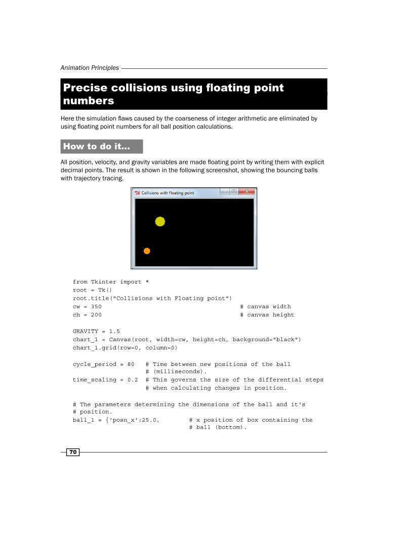
Animation Principles
�0
Precise collisions using floating point numbers
Here the simulation flaws caused by the coarseness of integer arithmetic are eliminated by using floating point numbers for all ball position calculations.
How to do it...All position, velocity, and gravity variables are made floating point by writing them with explicit decimal points. The result is shown in the following screenshot, showing the bouncing balls with trajectory tracing.
from Tkinter import *root = Tk()root.title("Collisions with Floating point")cw = 350 # canvas widthch = 200 # canvas height
GRAVITY = 1.5chart_1 = Canvas(root, width=cw, height=ch, background="black")chart_1.grid(row=0, column=0)
cycle_period = 80 # Time between new positions of the ball # (milliseconds).time_scaling = 0.2 # This governs the size of the differential steps # when calculating changes in position.
# The parameters determining the dimensions of the ball and it's # position.ball_1 = {'posn_x':25.0, # x position of box containing the # ball (bottom).

Chapter 4
�1
'posn_y':180.0, # x position of box containing the # ball (left edge). 'velocity_x':30.0, # amount of x-movement each cycle of # the 'for' loop. 'velocity_y':100.0, # amount of y-movement each cycle of # the 'for' loop. 'ball_width':20.0, # size of ball - width (x-dimension). 'ball_height':20.0, # size of ball - height (y-dimension). 'color':"dark orange", # color of the ball 'coef_restitution':0.90} # proportion of elastic energy # recovered each bounce
ball_2 = {'posn_x':cw - 25.0, 'posn_y':300.0, 'velocity_x':-50.0, 'velocity_y':150.0, 'ball_width':30.0, 'ball_height':30.0, 'color':"yellow3", 'coef_restitution':0.90}
def detectWallCollision(ball): # Collision detection with the walls of the container if ball['posn_x'] > cw - ball['ball_width']: # Collision # with right-hand wall. ball['velocity_x'] = -ball['velocity_x'] * ball['coef_ \ restitution'] # reverse direction. ball['posn_x'] = cw - ball['ball_width'] if ball['posn_x'] < 1: # Collision with left-hand wall. ball['velocity_x'] = -ball['velocity_x'] * ball['coef_ \restitution'] ball['posn_x'] = 2 # anti-stick to the wall if ball['posn_y'] < ball['ball_height'] : # Collision # with ceiling. ball['velocity_y'] = -ball['velocity_y'] * ball['coef_ \ restitution'] ball['posn_y'] = ball['ball_height'] if ball['posn_y'] > ch - ball['ball_height']: # Floor # collision. ball['velocity_y'] = - ball['velocity_y'] * ball['coef_ \restitution'] ball['posn_y'] = ch - ball['ball_height']
def diffEquation(ball): # An approximate set of differential equations of motion # for the balls ball['posn_x'] += ball['velocity_x'] * time_scaling ball['velocity_y'] = ball['velocity_y'] + GRAVITY # a crude # equation incorporating gravity.

Animation Principles
�2
ball['posn_y'] += ball['velocity_y'] * time_scaling chart_1.create_oval( ball['posn_x'], ball['posn_y'], ball['posn_x'] + ball['ball_width'],\ ball ['posn_y'] + ball['ball_height'], \ fill= ball['color']) detectWallCollision(ball) # Has the ball collided with # any container wall?
for i in range(1,2000): # end the program after 1000 position shifts.
diffEquation(ball_1) diffEquation(ball_2)
chart_1.update() # This refreshes the drawing on the canvas. chart_1.after(cycle_period) # This makes execution pause for 200 # milliseconds. chart_1.delete(ALL) # This erases everything on theroot.mainloop()
How it works...Use of precision arithmetic has allowed us to notice simulation behavior that was previously hidden by the sins of integer-only calculations. This is the UNIQUE VALUE OF GRAPHIC SIMULATION AS A DEBUGGING TOOL. If you can represent your ideas in a visual way rather than as lists of numbers you will easily pick up subtle quirks in your code. The human brain is designed to function best in graphical images. It is a direct consequence of being a hunter.
A graphic debugging tool...There is another very handy trick in the software debugger's arsenal and that is the visual trace. A trace is some kind of visual trail that shows the history of dynamic behavior. All of this is revealed in the next example.
Trajectory tracing and ball-to-ball collisionsNow we introduce one of the more difficult behaviors in our simulation of ever increasing complexity – the mid-air collision.
The hardest thing when you are debugging a program is to try to hold in your short term memory some recently observed behavior and compare it meaningfully with present behavior. This kind of memory is an imperfect recorder. The way to overcome this is to create a graphic form of memory – some sort of picture that shows accurately what has been happening in the past. In the same way that military cannon aimers use glowing tracer projectiles to adjust their aim, a graphic programmer can use trajectory traces to examine the history of execution.

Chapter 4
�3
How to do it...In our new code there is a new function called detect_ball_collision (ball_1, ball_2) whose job is to anticipate imminent collisions between the two balls no matter where they are. The collisions will come from any direction and therefore we need to be able to test all possible collision scenarios and examine the behavior of each one and see if it does not work as planned. This can be too difficult unless we create tools to test the outcome. In this recipe, the tool for testing outcomes is a graphic trajectory trace. It is a line that trails behind the path of the ball and shows exactly where it went right since the beginning of the simulation. The result is shown in the following screenshot, showing the bouncing with ball-to-ball collision rebounds.
# kinetic_gravity_balls_1.py# >>>>>>>>>>>>>>>>>>>>>>>>>>>>>>>>>>>>>>>>>>>>>>>>>>from Tkinter import *import mathroot = Tk()root.title("Balls bounce off each other")cw = 300 # canvas widthch = 200 # canvas height
GRAVITY = 1.5 chart_1 = Canvas(root, width=cw, height=ch, background="white")chart_1.grid(row=0, column=0)
cycle_period = 80 # Time between new positions of the ball # (milliseconds).time_scaling = 0.2 # The size of the differential steps
# The parameters determining the dimensions of the ball and its # position.

Animation Principles
�4
ball_1 = {'posn_x':25.0, 'posn_y':25.0, 'velocity_x':65.0, 'velocity_y':50.0, 'ball_width':20.0, 'ball_height':20.0, 'color':"SlateBlue1", 'coef_restitution':0.90}
ball_2 = {'posn_x':180.0, 'posn_y':ch- 25.0, 'velocity_x':-50.0, 'velocity_y':-70.0, 'ball_width':30.0, 'ball_height':30.0, 'color':"maroon1", 'coef_restitution':0.90}
def detect_wall_collision(ball): # detect ball-to-wall collision if ball['posn_x'] > cw - ball['ball_width']: # Right-hand wall. ball['velocity_x'] = -ball['velocity_x'] * ball['coef_ \restitution'] ball['posn_x'] = cw - ball['ball_width'] if ball['posn_x'] < 1: # Left-hand wall. ball['velocity_x'] = -ball['velocity_x'] * ball['coef_ \restitution'] ball['posn_x'] = 2 if ball['posn_y'] < ball['ball_height'] : # Ceiling. ball['velocity_y'] = -ball['velocity_y'] * ball['coef_ \restitution'] ball['posn_y'] = ball['ball_height'] if ball['posn_y'] > ch - ball['ball_height'] : # Floor ball['velocity_y'] = - ball['velocity_y'] * ball['coef_ \restitution'] ball['posn_y'] = ch - ball['ball_height']
def detect_ball_collision(ball_1, ball_2): #detect ball-to-ball collision # firstly: is there a close approach in the horizontal direction if math.fabs(ball_1['posn_x'] - ball_2['posn_x']) < 25: # secondly: is there also a close approach in the vertical # direction.
Dow
nlo
ad fro
m W
ow
! eBook
<w
ww
.wow
ebook.
com
>

Chapter 4
�5
if math.fabs(ball_1['posn_y'] - ball_2['posn_y']) < 25: ball_1['velocity_x'] = -ball_1['velocity_x'] # reverse # direction. ball_1['velocity_y'] = -ball_1['velocity_y'] ball_2['velocity_x'] = -ball_2['velocity_x'] ball_2['velocity_y'] = -ball_2['velocity_y'] # to avoid internal rebounding inside balls ball_1['posn_x'] += ball_1['velocity_x'] * time_scaling ball_1['posn_y'] += ball_1['velocity_y'] * time_scaling ball_2['posn_x'] += ball_2['velocity_x'] * time_scaling ball_2['posn_y'] += ball_2['velocity_y'] * time_scaling
def diff_equation(ball): x_old = ball['posn_x'] y_old = ball['posn_y'] ball['posn_x'] += ball['velocity_x'] * time_scaling ball['velocity_y'] = ball['velocity_y'] + GRAVITY ball['posn_y'] += ball['velocity_y'] * time_scaling chart_1.create_oval( ball['posn_x'], ball['posn_y'],\ ball['posn_x'] + ball['ball_width'],\ ball['posn_y'] + ball['ball_height'],\ fill= ball['color'], tags="ball_tag") chart_1.create_line( x_old, y_old, ball['posn_x'], \ ball ['posn_y'], fill= ball['color']) detect_wall_collision(ball) # Has the ball # collided with any container wall?
for i in range(1,5000): diff_equation(ball_1) diff_equation(ball_2) detect_ball_collision(ball_1, ball_2) chart_1.update() chart_1.after(cycle_period) chart_1.delete("ball_tag") # Erase the balls but # leave the trajectories
root.mainloop()

Animation Principles
�6
How it works...Mid-air ball against ball collisions are done in two steps. In the first step, we test whether the two balls are close to each other inside a vertical strip defined by if math.fabs(ball_1['posn_x'] - ball_2['posn_x']) < 25. In plain English, this asks "Is the horizontal distance between the balls less than 25 pixels?" If the answer is yes, then the region of examination is narrowed down to a small vertical distance less than 25 pixels by the statement if math.fabs(ball_1['posn_y'] - ball_2['posn_y']) < 25. So every time the loop is executed, we sweep the entire canvas to see if the two balls are both inside an area where their bottom-left corners are closer than 25 pixels to each other. If they are that close then we simply cause a rebound off each other by reversing their direction of travel in both the horizontal and vertical directions.
There's more...Simply reversing the direction is not the mathematically correct way to reverse the direction of colliding balls. Certainly billiard balls do not behave that way. The law of physics that governs colliding spheres demands that momentum be conserved. This requires more complicated mathematics not covered in this book.
Why do we sometimes get tkinter.TckErrors?If we click the close window button (the X in the top right) while Python is paused, when Python revives and then calls on Tcl (Tkinter) to draw something on the canvas we will get an error message. What probably happens is that the application has already shut down, but Tcl has unfinished business. If we allow the program to run to completion before trying to shut the window then termination is orderly.
Rotating lineNow we will see how to handle rotating lines. In any kind of graphic computer work, the need to rotate objects arises eventually. By starting off as simply as possible and progressively adding behaviors we can handle some increasingly complicated situations. This recipe is that first simple step in the art of making things rotate.
Getting readyTo understand the mathematics of rotation you need to be reasonably familiar with the trigonometry functions of sine, cosine, and tangent. The good news for those of us whose eyes glaze at the mention of trigonometry is that you can use these examples without understanding trigonometry. However, it is much more rewarding if you do try to figure out the math. It is like the difference between watching football or playing it. Only the players get fit.
Chapter 4
��
How to do it...You just need to write and run this code and observe the results as you did for all the other recipes. The insights come from repeated tinkering and hacking the code. Change the values of variables p1_x to p2_y one at a time and observe the results.
# rotate_line_1.py#>>>>>>>>>>>>>>>>>>>>>>>>>>>>>>>>>>>>>>>>>>from Tkinter import *import mathroot = Tk()root.title("Rotating line")cw = 220 # canvas widthch = 180 # canvas heightchart_1 = Canvas(root, width=cw, height=ch, background="white")chart_1.grid(row=0, column=0)cycle_period = 50 # pause duration (milliseconds).
p1_x = 90.0 # the pivot pointp1_y = 90.0 # the pivot point,p2_x = 180.0 # the specific point to be rotatedp2_y = 160.0 # the specific point to be rotated.
a_radian = math.atan((p2_y - p1_y)/(p2_x - p1_x))a_length = math.sqrt((p2_y - p1_y)*(p2_y - p1_y) +\ (p2_x - p1_x)*(p2_x - p1_x))
for i in range(1,300): # end the program after 300 position shifts a_radian +=0.05 # incremental rotation of 0.05 radians p1_x = p2_x - a_length * math.cos(a_radian) p1_y = p2_y - a_length * math.sin(a_radian) chart_1.create_line(p1_x, p1_y, p2_x, p2_y) chart_1.update() chart_1.after(cycle_period) chart_1.delete(ALL)
root.mainloop()
How it works...In essence, all rotation comes down to the following:
Establish a center of rotation or pivot point
Pick a specific point on the object you want to rotate
Animation Principles
��
Calculate the distance from the pivot point to the specific point of interest
Calculate the angle of the line joining the pivot and the specific point
Increase the angle of the line joining the points by a known amount, the rotation angle, and re-calculate the new x and y coordinates for that point.
For math students what you do is relocate the origin of your rectangular coordinate system to the pivot point, express the coordinates of your specific point into polar coordinates, add an increment to the angular position, and convert the new polar coordinate position into a fresh pair of rectangular coordinates. The preceding recipe performs all these actions.
There's more...The pivot point was purposely placed near the bottom corner of the canvas so that the point on the end of the line to be rotated would fall outside the canvas for much of the rotation process. The rotation continues without errors or bad behavior emphasizing a point made earlier in this chapter that Python is mathematically robust. However, we need to exercise care when using the arctangent function math.atan() because it flips from a value positive infinity to negative infinity as angles move through 90 and 270 degrees. Atan() can give ambiguous results. Again the Python designers have taken care of business well by creating the math. atan2(y,x) function that takes into account the signs of both y and x to give unambiguous results between 180 degrees and -180.
Trajectory tracing on multiple line rotationsThis example draws a visually appealing kind of Art Noveau arrowhead but that is just an issue on the happy-side. The real point of this recipe is to see how you can have any number of pivot points all with different motions and that the essential arithmetic remains simple and clean looking in Python. The use of animation methods to slow the execution down makes it entertaining to watch. We also see how tag names given to different parts of the objects drawn onto the canvas allow them to be selectively erased when the canvas.delete(...) method is invoked.
Getting readyImagine a skilled drum major marching in a parade whirling a staff in circles. Holding onto the end of the staff is a small monkey also twirling a baton but at a different speed. At the tip of the monkey's staff is a miniature marmoset twirling a baton in the opposite direction...
Now run the program.
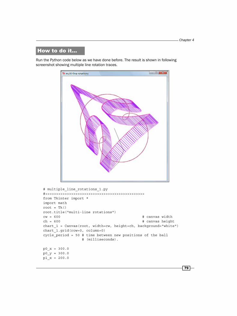
Chapter 4
��
How to do it...Run the Python code below as we have done before. The result is shown in following screenshot showing multiple line rotation traces.
# multiple_line_rotations_1.py#>>>>>>>>>>>>>>>>>>>>>>>>>>>>>>>>>>>>>>>>>>>>>>from Tkinter import *import mathroot = Tk()root.title("multi-line rotations")cw = 600 # canvas widthch = 600 # canvas heightchart_1 = Canvas(root, width=cw, height=ch, background="white")chart_1.grid(row=0, column=0)cycle_period = 50 # time between new positions of the ball # (milliseconds).
p0_x = 300.0p0_y = 300.0p1_x = 200.0

Animation Principles
�0
p1_y = 200.0p2_x = 150.0 # central pivotp2_y = 150.0 # central pivotp3_x = 100.0p3_y = 100.0p4_x = 50.0p4_y = 50.0
alpha_0 = math.atan((p0_y - p1_y)/(p0_x - p1_x))length_0_1 = math.sqrt((p0_y - p1_y)*(p0_y - p1_y) +\ (p0_x - p1_x)*(p0_x - p1_x))
alpha_1 = math.atan((p1_y - p2_y)/(p1_x - p2_x))length_1_2 = math.sqrt((p2_y - p1_y)*(p2_y - p1_y) +\ (p2_x - p1_x)*(p2_x - p1_x))
alpha_2 = math.atan((p2_y - p3_y)/(p2_x - p3_x))length_2_3 = math.sqrt((p3_y - p2_y)*(p3_y - p2_y) +\ (p3_x - p2_x)*(p3_x - p2_x))
alpha_3 = math.atan((p3_y - p4_y)/(p3_x - p4_x))length_3_4 = math.sqrt((p4_y - p3_y)*(p4_y - p3_y) +\ (p4_x - p3_x)*(p4_x - p3_x))
for i in range(1,5000): alpha_0 += 0.1 alpha_1 += 0.3 alpha_2 -= 0.4 p1_x = p0_x - length_0_1 * math.cos(alpha_0) p1_y = p0_y - length_0_1 * math.sin(alpha_0)
tip_locus_2_x = p2_x tip_locus_2_y = p2_y p2_x = p1_x - length_1_2 * math.cos(alpha_1) p2_y = p1_y - length_1_2 * math.sin(alpha_1)
tip_locus_3_x = p3_x tip_locus_3_y = p3_y p3_x = p2_x - length_2_3 * math.cos(alpha_2) p3_y = p2_y - length_2_3 * math.sin(alpha_2)
Chapter 4
�1
tip_locus_4_x = p4_x tip_locus_4_y = p4_y p4_x = p3_x - length_3_4 * math.cos(alpha_3) p4_y = p3_y - length_3_4 * math.sin(alpha_3)
chart_1.create_line(p1_x, p1_y, p0_x, p0_y, tag='line_1') chart_1.create_line(p2_x, p2_y, p1_x, p1_y, tag='line_2') chart_1.create_line(p3_x, p3_y, p2_x, p2_y, tag='line_3') chart_1.create_line(p4_x, p4_y, p3_x, p3_y, fill="purple", \tag='line_4')
# Locus tip_locus_2 at tip of line 1-2 chart_1.create_line(tip_locus_2_x, tip_locus_2_y, p2_x, p2_y, \ fill='maroon') # Locus tip_locus_2 at tip of line 2-3 chart_1.create_line(tip_locus_3_x, tip_locus_3_y, p3_x, p3_y, \ fill='orchid1') # Locus tip_locus_2 at tip of line 2-3 chart_1.create_line(tip_locus_4_x, tip_locus_4_y, p4_x, p4_y, \ fill='DeepPink')
chart_1.update() chart_1.after(cycle_period) chart_1.delete('line_1', 'line_2', 'line_3')
root.mainloop()
How it works...As we did in the previous recipe we have lines defined by connecting two points, each being specified in the rectangular coordinates that Tkinter drawing methods use. There are three such lines connected pivot-to-tip. It may help to visualize each pivot as a drum major or a monkey. We convert each pivot-to-tip line into polar coordinates of length and angle. Then each pivot-to-tip line is rotated by its own individual increment angle. If you alter these angles alpha_1 etc. or the positions of the various pivot points you will get a limitless variety of interesting patterns.
There's more...Once you are able to control and vary color you are able to make extraordinary and beautiful patterns never seen before. Color control is the subject of the next chapter.

Animation Principles
�2
A rose for youThis last example of the chapter is simply a gift for the reader. No illustration is provided. We will only see the result if we run the code. It is a surprise.
from Tkinter import *root = Tk()root.title("This is for you dear reader. A token of esteem and affection.")import math
cw = 800 # canvas widthch = 800 # canvas height
chart_1 = Canvas(root, width=cw, height=ch, background="black")chart_1.grid(row=0, column=0)
p0_x = 400.0p0_y = 400.0
p1_x = 330.0p1_y = 330.0
p2_x = 250.0p2_y = 250.0
p3_x = 260.0p3_y = 260.0
p4_x = 250.0p4_y = 250.0
p5_x = 180.0p5_y = 180.0
alpha_0 = math.atan((p0_y - p1_y)/(p0_x - p1_x))length_0_1 = math.sqrt((p0_y - p1_y)*(p0_y - p1_y) + (p0_x - p1_ \x)*(p0_x - p1_x))
alpha_1 = math.atan((p1_y - p2_y)/(p1_x - p2_x))length_1_2 = math.sqrt((p2_y - p1_y)*(p2_y - p1_y) + (p2_x - p1_ \x)*(p2_x - p1_x))

Chapter 4
�3
alpha_2 = math.atan((p2_y - p3_y)/(p2_x - p3_x))length_2_3 = math.sqrt((p3_y - p2_y)*(p3_y - p2_y) + (p3_x - p2_ \ x)*(p3_x - p2_x))
alpha_3 = math.atan((p3_y - p4_y)/(p3_x - p4_x))length_3_4 = math.sqrt((p4_y - p3_y)*(p4_y - p3_y) + (p4_x - p3_ \ x)*(p4_x - p3_x))
alpha_4 = math.atan((p3_y - p5_y)/(p3_x - p5_x))length_4_5 = math.sqrt((p5_y - p4_y)*(p5_y - p4_y) + (p5_x - p4_ \x)*(p5_x - p4_x))
for i in range(1,2300): # end the program after 500 position # shifts.
alpha_0 += 0.003 alpha_1 += 0.018 alpha_2 -= 0.054 alpha_3 -= 0.108 alpha_4 += 0.018
p1_x = p0_x - length_0_1 * math.cos(alpha_0) p1_y = p0_y - length_0_1 * math.sin(alpha_0)
tip_locus_2_x = p2_x tip_locus_2_y = p2_y p2_x = p1_x - length_1_2 * math.cos(alpha_1) p2_y = p1_y - length_1_2 * math.sin(alpha_1)
tip_locus_3_x = p3_x tip_locus_3_y = p3_y p3_x = p2_x - length_2_3 * math.cos(alpha_2) p3_y = p2_y - length_2_3 * math.sin(alpha_2)
tip_locus_4_x = p4_x tip_locus_4_y = p4_y p4_x = p3_x - length_3_4 * math.cos(alpha_3) p4_y = p3_y - length_3_4 * math.sin(alpha_3)
tip_locus_5_x = p5_x tip_locus_5_y = p5_y p5_x = p4_x - length_4_5 * math.cos(alpha_4) p5_y = p4_y - length_4_5 * math.sin(alpha_4)
Animation Principles
�4
chart_1.create_line(p1_x, p1_y, p0_x, p0_y, tag='line_1', \ fill='gray') chart_1.create_line(p2_x, p2_y, p1_x, p1_y, tag='line_2', \ fill='gray') chart_1.create_line(p3_x, p3_y, p2_x, p2_y, tag='line_3', \ fill='gray') chart_1.create_line(p4_x, p4_y, p3_x, p3_y, tag='line_4', \ fill='gray') chart_1.create_line(p5_x, p5_y, p4_x, p4_y, tag='line_5', \ fill='#550000')
chart_1.create_line(tip_locus_2_x, tip_locus_2_y, p2_x, p2_y, \ fill='#ff00aa') chart_1.create_line(tip_locus_3_x, tip_locus_3_y, p3_x, p3_y, \ fill='#aa00aa') chart_1.create_line(tip_locus_4_x, tip_locus_4_y, p4_x, p4_y, \ fill='#dd00dd') chart_1.create_line(tip_locus_5_x, tip_locus_5_y, p5_x, p5_y, \ fill='#880066') chart_1.create_line(tip_locus_2_x, tip_locus_2_y, p5_x, p5_y, \ fill='#0000ff') chart_1.create_line(tip_locus_3_x, tip_locus_3_y, p4_x, p4_y, \ fill='#6600ff')
chart_1.update() # This refreshes the drawing on the # canvas. chart_1.delete('line_1', 'line_2', 'line_3', 'line_4') # Erase # selected tags.
root.mainloop()
How it works...The structure of this program is similar to the previous example but the rotation parameters have been adjusted to evoke the image of a rose. The colors used are chosen to remind us that control over color is extremely import in graphics.

5The Magic of Color
In this chapter, we will cover:
A limited palette of named colors
Nine ways of specifying color
A ball of varying shades of red
A red color wedge of graded hue
The artist's color wheel (Newton's Color Wheel)
The numerical color mixing-matching palette
The animated graded color wheel
Tkinter's own color mixer-picker
IntroductionTkinter allows you to use more than 16 million colors. That is 256 levels each of red, green, and blue added together. There are two main ways of specifying colors: by name, or as a hexadecimal value packed together as a string. A competent color expert can create any color possible by mixing red, green, and blue in varying amounts. There are accepted rules and conventions for what constitutes pleasing and tasteful color combinations. Sometimes you want to make shaded blends of colors and at other times you just want to use a limited number of colors with the minimum amount of both. We deal with these issues in this chapter.

The Magic of Color
�6
A limited palette of named colorsThere is a vast list of romantically named colors like cornflower blue, misty rose, or papaya whip. There are about 340 of these named colors that are usable in Python.
Colors get names because people remember them most easily in association with a place and an emotional mood. It is easy to remember evocative names and therefore easier to use them. In this example, we reduce the long list down to 140 by using systematic names and eliminating colors that are very similar.
How to do it...Execute the program shown in exactly the same way as all the examples in previous chapters. What you should see on your screen is a logically laid out chart of rectangular color swatches. Each will have its callable name on it. These are names you can use in Python/Tkinter programs and they will be correctly displayed.
#systematic_colorNames_1.py#>>>>>>>>>>>>>>>>>>>>>>>>>>>>>>>>>>>>>>>>>>>>>>from Tkinter import *root = Tk()root.title("Systematically named colors - limited pallette")cw = 1000 # canvas widthch = 800 # canvas heightcanvas_1 = Canvas(root, width=cw, height=ch, background="black")canvas_1.grid(row=0, column=1)
whiteColors = "Gainsboro","peach puff","cornsilk",\"honeydew","aliceblue","misty rose","snow", "snow3","snow4",\"SlateGray1", "SlateGray3", "SlateGray4",\"gray", "darkGray","DimGray","DarkSlateGray"
redColors = "Salmon","salmon1","salmon2","salmon3","salmon4",\"orange red","OrangeRed2","OrangeRed3","OrangeRed4",\"red","red3","red4",\"IndianRed1","IndianRed3","IndianRed4",\"firebrick","firebrick1","firebrick3","firebrick4",\"sienna","sienna1","sienna3","sienna4"
pinkColors = "Pink","pink3","pink4",\"hot pink","HotPink3","HotPink4",\"deep pink","DeepPink3","DeepPink4",\"PaleVioletRed1","PaleVioletRed2","PaleVioletRed3","PaleVioletRed4",\"maroon","maroon1","maroon3","maroon4"
Dow
nlo
ad fro
m W
ow
! eBook
<w
ww
.wow
ebook.
com
>

Chapter 5
��
magentaColors = "magenta","magenta3","magenta4","DarkMagenta",\"orchid1","orchid3","orchid4",\"MediumOrchid3","MediumOrchid4",\"DarkOrchid","DarkOrchid1","DarkOrchid4",\"MediumPurple1","MediumPurple3", "MediumPurple4",\"purple","purple3","purple4"
blueColors = "blue","blue3","blue4",\"SlateBlue1", "SlateBlue3","SlateBlue4",\"DodgerBlue2", "DodgerBlue3","DodgerBlue4",\"deep sky blue","DeepSkyBlue3", "DeepSkyBlue4",\"sky blue", "SkyBlue3", "SkyBlue4"
cyanColors = "CadetBlue1", "CadetBlue3", "CadetBlue4",\"pale turquoise", "PaleTurquoise3","PaleTurquoise4",\"cyan", "cyan3", "cyan4",\"aquamarine","aquamarine3", "aquamarine4"
greenColors = "green", "green3", "green4","dark green",\"chartreuse", "chartreuse3", "chartreuse4",\"SeaGreen","SeaGreen1", "SeaGreen3",\"pale green", "PaleGreen3", "PaleGreen4",\"spring green", "SpringGreen3", "SpringGreen4",\"olive drab","OliveDrab1", "OliveDrab4",\"dark olive green","DarkOliveGreen1", "DarkOliveGreen3", \ "DarkOliveGreen4",\
yellowColors= "yellow", "yellow3","yellow4",\"gold","gold3","gold4",\"goldenrod","goldenrod1","goldenrod3","goldenrod4",\"orange","orange3","orange4",\"dark orange","DarkOrange1","DarkOrange4"
x_start = 10y_start = 25x_width = 118x_offset = 2y_height = 30y_offset = 3text_offset = 0text_width = 95kbk = [x_start, y_start, x_start + x_width, y_start + y_height]

The Magic of Color
��
defshowColors(selectedColor):# Basic columnar color swatch display. All colours laid down in a # vertical stripe. print "number of colors --> ", len(selectedColor) for i in range (0,len(selectedColor)):kula = selectedColor[i] canvas_1.create_rectangle(kbk, fill=kula) canvas_1.create_text(kbk[0]+10, kbk[1] , text=kula, \ width=text_width, fill ="black", anchor=NW)kbk[1] += y_offset + y_height y0 = kbk[1]kbk[3] += y_offset + y_height y1 = kbk[3]kbk[1] = y_offset + y_heightkbk[3] = y_offset + 2 * y_heightkbk[0] += x_width + 2*x_offsetkbk[2] += x_width + 2*x_offset return y0,y1
showColors(redColors) showColors(pinkColors)showColors(magentaColors)showColors(cyanColors)showColors(blueColors) showColors(greenColors) showColors(yellowColors) showColors(whiteColors)
root.mainloop()#>>>>>>>>>>>>>>>>>>>>>>>>>>>>>>>>>>>>>>>>>>
How it works...
This program uses techniques developed in Chapter 2, Drawing Fundamental Shapes. There are eight lists of named colors grouped in color families with each family arranged in a logical sequence. The main technique was to use a general purpose function that would use a pre-defined rectangle and using a for loop, work through the list of color names in sequence. With each iteration of the loop, a rectangle is filled with that color and the color name is printed across it.

Chapter 5
��
There's more...These colors were chosen by trial and error to provide a reasonably wide palette suitable for most purposes. In the numbered sequences of colors like red where red1, red2, red3, and red4 represent increasingly darker shades, colors that are very similar to other colors in their neighborhood have been left out. It was also discovered that many colors were fake in that they are painted onto the canvas as grey.
The complete set of color names that Tkinter recognizes are found at http://wiki.tcl.tk/16166
To get fine shadings of the primary colorsTo achieve the subtle shadings and graduations of color combination, you need to mix the primary colors used on computer screens in controlled amounts. We begin this process in the next recipe.
A more compact color listAn even shorter sub-set of useful named colors are in the following color lists:
white_Colors = "white", "lemon chiffon", "honeydew","aliceblue","thistle", "misty rose"
blue_Colors = "blue","blue4","SlateBlue1","dodger blue","steelblue","sky blue"
grey_Colors ="SlateGray3", "SlateGray4", "LightGrey", "DarkGray", "DimGray", "LightSlateGray"
cyan_Colors = "CadetBlue1", "cyan", "cyan4", "LightSeaGreen", "aquamarine", "aquamarine3"
red_Colors = "light pink","IndianRed1","red","red2","red3","red4"
pink_Colors = "light pink","deeppink","hot pink","HotPink3","LightPink","LightPink2"
magenta_Colors = "PaleVioletRed1", "maroon", "maroon1", "magenta","magenta4", "orchid1"
purple_Colors = "purple", "purple4", "MediumPurple1", "plum2", "MediumOrchid", "DarkOrchid"
brown_Colors = "orange", "DarkOrange1", "DarkOrange2", "DarkOrange3", "DarkOrange4", "saddle brown"
green_Colors = "green", "green3", "green4"," chartreuse"," green yellow", "SpringGreen2"
yellow_Colors= "light yellow", "yellow", "yellow3","gold", "goldenrod1", "Khaki"
If you cut and paste these lists to replace the previous ones in systematic_colorNames_1.py, you will have a smaller, easier to manage, palette of 55 colors that you may find simpler to use.

The Magic of Color
�0
Nine ways of specifying colorWith this recipe we see an example of all the valid types of color specification. Basically there are two methods of specifying color that Tkinter recognizes, but there are a total of nine ways of expressing these. Thanks to the Python designers, the system is flexible and accepts all without complaint.
How to do it...
Execute the program shown in exactly the same way as all the examples in Chapter 2, Drawing Fundamental Shapes and you will see three disks filled with red and four with blue. Each is specified differently.
# color_arithmetic_1.py#>>>>>>>>>>>>>>>>>>>>>>>>>>>>>>>>>>>>>>>>>>from Tkinter import *root = Tk()root.title('Ways of Specifying Color')
cw = 270 # canvas widthch = 80 # canvas heightcanvas_1 = Canvas(root, width=cw, height=ch, background="white")canvas_1.grid(row=0, column=1)
# specify bottom-left and top-right as a set of four numbers named # 'xy'named_color_1 = "light blue" # oknamed_color_2 = "lightblue" # oknamed_color_3 = "LightBlue" # oknamed_color_4 = "Light Blue" # oknamed_color_5 = "Light Blue" # Name error - not ok: Tcl Error, # unknown color name
rgb_color = "rgb(255,0,0)" # Unknown color name.#rgb_percent_color = rgb(100%, 0%, 0%) # Invalid syntaxrgb_hex_1 = "#ff0000" # ok - 16.7 million colorsrgb_hex_2 = "#f00" # okrgb_hex_3 = "#ffff00000000" # ok - a ridiculous number
tk_rgb = "#%02x%02x%02x" % (128, 192, 200)printtk_rgby1, width, height = 20,20,20

Chapter 5
�1
canvas_1.create_oval(10,y1,10+width,y1+height, fill= rgb_hex_1)canvas_1.create_oval(30,y1,30+width,y1+height, fill= rgb_hex_2)canvas_1.create_oval(50,y1,50+width,y1+height, fill= rgb_hex_3)canvas_1.create_oval(70,y1,70+width,y1+height, fill= tk_rgb)y1 = 40canvas_1.create_oval(10,y1,10+width,y1+height, fill= named_color_1)canvas_1.create_oval(30,y1,30+width,y1+height, fill= named_color_2)canvas_1.create_oval(50,y1,50+width,y1+height, fill= named_color_3)canvas_1.create_oval(70,y1,70+width,y1+height, fill= named_color_4)root.mainloop()#>>>>>>>>>>>>>>>>>>>>>>>>>>>>>>>>>>>>>>>>>
How it works...Tkinter has the different name strings defined in a dictionary somewhere inside the Tkinter module library.
Converting color tuples to Tkinter Hex compatible specifiers
Some other languages specify colors as a numerical mixture of red, green and blue with each band ranging from 0 to 255 as a tuple. For example, pure red would be (255,0,0), pure green would be (0,255,0) and blue would be (0,0,255). A mixture of lots of red with a medium amount of green and just a touch of blue could be (230, 122, 20). These tuples are not recognized by Tkinter but the following line of Python code will convert any color_tuple into a color hex number that Tkinter will recognize and use as a color:
Tkinter_hex_color = '#%02x%02x%02x' % color_tuple,
where color_tuple = (230, 122, 20) or whatever numbers we choose to have in the tuple.
A red beachball of varying hueWe use the hexadecimal color specification scheme to make a series of color shades arranged in a pattern determined by predefined lists of numerical constants. The underlying idea is to establish a method of accessing these constants in a way that can be reused for quite different picture designs.

The Magic of Color
�2
How to do it...Execute the program shown in exactly the usual way, and you will see a sequence of colored disks laid on top of each other going from dark to light shades. The size and location of each disk is determined by the lists hFac and wFac. hfacisa mnemonic for " Height factor" andwFac for "Width factor". The following screenshot shows the Graded Color Ball.
# red_beach_ball_1.py# >>>>>>>>>>>>>>>>>from Tkinter import *root = Tk()root.title("Red beach ball")
cw = 240 # canvas widthch = 220 # canvas heightchart_1 = Canvas(root, width=cw, height=ch, background="black")chart_1.grid(row=0, column=0)
x_orig = 100y_orig = 200x_width = 80y_hite = 180
xy0 = [x_orig, y_orig]xy1 = [x_orig - x_width, y_orig - y_hite]xy2 = [x_orig + x_width, y_orig - y_hite ]wedge =[ xy0, xy1 , xy2 ]
width= 80 # Standard disk diameterhite = 80 # Median distance from origin (x_orig, y_orig).

Chapter 5
�3
hFac = [1.1, 1.15, 1.25, 1.35, 1.5, 1.6, 1.7] # Height # radial factors.wFac = [ 2.0, 1.9, 1.7, 1.4, 1.1, 0.75, 0.40] # Disk # diameter factors.# Color list. Elements incresing in darkness.kulaRed = ["#500000","#6e0000","#a00000","#ff0000",\ "#ff5050", "#ff8c8c", "#ffc8c8", "#ffffff" ]kula = kulaRed
for i in range(0, 7): # Red disks x0_disk = xy0[0] - width * wFac[i]/2 # Bottom left y0_disk = xy0[1] - hite * hFac[i] + width * wFac[i]/2xya = [x0_disk, y0_disk] # BOTTOM LEFT x1_disk = xy0[0] + width * wFac[i]/2 # Top right y1_disk = xy0[1] - hite * hFac[i] - width * wFac[i]/2xyb = [x1_disk, y1_disk] # TOP RIGHT chart_1.create_oval(xya ,xyb , fill=kula[i], outline=kula[i])
root.mainloop()
How it works...The series of images of varying shades of red disks is laid down in a specific sequence by a for loop. The matching shades of red are held in the sequenced list of hex colors. Hex is the short form for hexadecimal.
The variables used to specify the reference origin as well as all the other positional parameters have been set up so they can be reused in other patterns later. The important principle here is that with careful planning of our programming we only need to solve a problem once in a universal, designed-for-reuse way. Of course in practice this planned design takes more time and includes lot more experimentation than the simpler once-off way of writing code. Either way the whole experimental process starts off with writing messy, rough and ready code that 'kind-of' works. This initial rough work is a very necessary part of the creative process as it allows vaguely formed ideas to grow and evolve into effective software programs.
There's more...Having ironed out a scheme for drawing shaded disks in chosen geometric arrangements, we can now try different arrangements and end up with richer and more useful ideas. The next two recipes evolve this idea into a version of the artist's color wheel that illustrates how to achieve any color by controlled mixing of primary colors.

The Magic of Color
�4
A red color wedge of graded hueWe create a wedge-shaped segment to form a logical pattern that can be incorporated into a wheel arrangement intended to show the relationships between different colors.
How to do it...The code structure used in the previous recipe is re-used here. When you execute the following code you will see a neat row of colored disks laid onto a dark shaded triangular wedge going from dark to light shades of red. The following screenshot shows the Graded Color Wedge.
# red_color_segment_1.py#>>>>>>>>>>>>>>>>>>>from Tkinter import *root = Tk()root.title("Red color wedge")cw = 240 # canvas widthch = 220 # canvas heightchart_1 = Canvas(root, width=cw, height=ch, background="white")chart_1.grid(row=0, column=0)
theta_deg = 0.0x_orig = 100y_orig = 200x_width = 80y_hite = 180
xy0 = [x_orig, y_orig]xy1 = [x_orig - x_width, y_orig - y_hite]
Chapter 5
�5
xy2 = [x_orig + x_width, y_orig - y_hite ]wedge =[ xy0, xy1 , xy2 ]
width= 40 #standard disk diameterhite = 80 # median wedge height.hFac = [0.25, 0.45, 0.75, 1.2, 1.63, 1.87, 2.05] # Radial # factorswFac = [ 0.2, 0.36, 0.6, 1.0, 0.5, 0.3, 0.25] # disk # diameter factors
# Color list. Elements increasing in darkness.kulaRed = ["#000000","#6e0000","#a00000","#ff0000",\ "#ff5050", "#ff8c8c", "#ffc8c8", \ "#440000" ] kula = kulaRed
wedge =[ xy0, xy1 , xy2 ] # black backgroundchart_1.create_polygon(wedge,fill=kula[0])
x_width = 40 # dark red wedgey_hite = 160xy1 = [x_orig - x_width, y_orig - y_hite]xy2 = [x_orig + x_width, y_orig - y_hite ]wedge =[ xy0, xy1 , xy2 ]chart_1.create_polygon(wedge,fill=kula[1])
for i in range(0, 7): # red disks x0_disk = xy0[0] - width * wFac[i]/2 # bottom left y0_disk = xy0[1] - hite * hFac[i] + width * wFac[i]/2xya = [x0_disk, y0_disk] # BOTTOM LEFT x1_disk = xy0[0] + width * wFac[i]/2 # top right y1_disk = xy0[1] - hite * hFac[i] - width * wFac[i]/2xyb = [x1_disk, y1_disk] #TOP RIGHT chart_1.create_oval(xya ,xyb , fill=kula[i], outline=kula[i])
root.mainloop()
How it works...By adjusting the numerical values in the lists hFac and wFac, we arrange the colored disks to fit inside a background wedge that happens to be the correct shape to form a one-twelfth pie slice of a circle.

The Magic of Color
�6
There's more...The way we have named and re-renamed the color list kula seems redundant and therefore perhaps confusing. However, the method in this apparent madness is that if we had many other lists of colors to use at the same time, it then becomes much simpler to reuse existing methods.
Newton's grand wheel of color mixingWe make a version of the artist's color wheel which shows how any known color and shade of color can be obtained by judicious mixing of the three primary colors of red, green and blue.
How to do it...We have made a set of twelve color lists. Each list represents the color that results when you mix colors on either side of it, except for the primary colors of red, green, and blue. The other critical addition to the code is the function rotate(xya, xyb, theta_deg_incr) that is used to rotate the color wedge pattern to a new chosen position around a central point. As some trigonometry is used to do the rotation, the math module needs to be imported at the top of the code. Each segment forms part of the complete circle of color variations. The following screenshot shows a version of Isaac Newton's Color Wheel.

Chapter 5
��
# primary_color_wheel_1.py#>>>>>>>>>>>>>>>>>>>>>from Tkinter import *import mathroot = Tk()root.title("Color wheel segments")cw = 400 # canvas widthch = 400 # canvas heightchart_1 = Canvas(root, width=cw, height=ch, background="black")chart_1.grid(row=0, column=0)
theta_deg = 0.0x_orig = 200y_orig = 200x_width = 40y_hite = 160
xy0 = [x_orig, y_orig]xy1 = [x_orig - x_width, y_orig - y_hite]xy2 = [x_orig + x_width, y_orig - y_hite ]wedge =[ xy0, xy1 , xy2 ]
width= 40 #standard disk diameterhite = 80 # median wedge height.hFac = [0.25, 0.45, 0.75, 1.2, 1.63, 1.87, 2.05] # Radial # factorswFac = [ 0.2, 0.36, 0.6, 1.0, 0.5, 0.3, 0.25] # disk # diameter factorsx_DiskRot = [1.0, 1.0, 1.0, 1.0, 1.0, 1.0, 1.0] # rotational coordinatesy_DiskRot = [1.0, 1.0, 1.0, 1.0, 1.0, 1.0, 1.0]
#REDkulaRed = ["#000000", "#6e0000", "#a00000", "#ff0000",\ "#ff5050", "#ff8c8c", "#ffc8c8", \ "#440000" ]# KhakikulaRRedGreen = ["#000000", "#606000", "#8f9f00", "#b3b300",\ "#d6d600", "#dbdb30", \ "#dbdb77", "#3e2700" ]# YellowkulaRedGreen = ["#000000", "#6e6e00", "#a0a000", "#ffff00",\ "#ffff50", "#ffff8c", \ "#ffffc8", "#444400" ] # OrangekulaRedGGreen = ["#000000", "#493100", "#692f00", "#a25d00",\

The Magic of Color
��
"#ff8300", "#ffa55a", \ "#ffb681", "#303030" ] # GreenkulaGreen = ["#000000", "#006e00", "#00a000", "#00ff00",\ "#50ff50", "#8cff8c", "#c8ffc8", \ "#004400" ] # Dark greenkulaGGreenBlue = ["#000000", "#003227", "#009358", "#00a141",\ "#00ff76", "#72ff99", \ "#acffbf", "#003a1d" ] # CyankulaGreenBlue = ["#000000", "#006e6e", "#00a0a0", "#00ffff",\ "#50ffff", "#8cffff", \ "#c8ffff", "#004444" ]# Steel BluekulaGreenBBlue = ["#000000", "#002c46", "#00639c", "#008cc8",\ "#00b6ff", "#7bb6ff", \ "#addfff", "#001a27" ]# BluekulaBlue = ["#000000", "#00006e", "#0000a0", "#0000ff",\ "#5050ff", "#8c8cff", "#c8c8ff", \ "#000044" ]# PurplekulaBBlueRed = ["#000000", "#470047", "#6c00a2", "#8f00ff",\ "#b380ff", "#d8b3ff", "#f1deff", \ "#200031" ]# CrimsonkulaBlueRed = ["#000000", "#6e006e", "#a000a0", "#ff00ff",\ "#ff50ff", "#ff8cff", "#ffc8ff", \ "#440044" ]# MagentakulaBlueRRed = ["#000000", "#380023", "#80005a", "#b8007b",\ "#ff00a1", "#ff64c5", "#ff89ea", \ "#2e0018" ]
# ROTATEdef rotate(xya, xyb, theta_deg_incr): #xya, xyb are 2 component # points # General purpose point rotation functiontheta_rad = math.radians(theta_deg_incr)a_radian = math.atan2( (xyb[1] - xya[1]) , (xyb[0] - xya[0]) )a_length = math.sqrt( (xyb[1] - xya[1])**2 + (xyb[0] - xya[0])**2)theta_rad += a_radiantheta_deg = math.degrees(theta_rad)new_x = a_length * math.cos(theta_rad)new_y = a_length * math.sin(theta_rad) return new_x, new_y, theta_deg # theta_deg = post # rotation angle
Dow
nlo
ad fro
m W
ow
! eBook
<w
ww
.wow
ebook.
com
>

Chapter 5
��
# GENL. SEGMENT BACKGROUND FUNCTIONdefsegmentBackground(kula, angle, xy1, xy2): xy_new1 = rotate(xy0, xy1, angle) # rotate xy1 xy1 =[ xy_new1[0] + xy0[0], xy_new1[1] + xy0[1] ] xy_new2 = rotate(xy0, xy2, angle) # rotate xy2 xy2 =[ xy_new2[0] + xy0[0], xy_new2[1] + xy0[1] ] wedge =[ xy0, xy1 , xy2 ] chart_1.create_polygon(wedge,fill=kula[7])
# GENL. COLOR DISKS FUNCTIONdefcolorDisks( kula, angle): global hite, width, hFac, wFac for i in range(0, 7): # green segment disksxya = [xy0[0], xy0[1] - hite * hFac[i] ] # position of point for # rotation xy_new1 = rotate(xy0, xya, angle) # rotate xya # NEW CIRCLE CENTERS AFTER ROTATION OF CENTERLINE x0_disk = xy_new1[0] + xy0[0] - width*wFac[i]/2 y0_disk = xy_new1[1] + xy0[1] + width * wFac[i]/2xya = [x0_disk, y0_disk] # BOTTOM LEFT x1_disk = xy_new1[0] + xy0[0] + width*wFac[i]/2 y1_disk = xy_new1[1] + xy0[1] - width * wFac[i]/2xyb = [x1_disk, y1_disk] #TOP RIGHT chart_1.create_oval(xya ,xyb , fill=kula[i], outline=kula[i])
for i in range(0,12): if i==0: angle = 0.0kula = kulaRed if i==1: angle = 30.0kula = kulaRRedGreen if i==2: angle = 60.0kula = kulaRedGreen if i==3: angle = 90.0kula = kulaRedGGreen if i==4: angle = 120.0kula = kulaGreen if i==5: angle = 150.0kula = kulaGGreenBlue if i==6: angle = 180.0kula = kulaGreenBlue

The Magic of Color
100
if i==7: angle = 210.0kula = kulaGreenBBlue if i==8: angle = 240.0kula = kulaBlue if i==9: angle = 270.0kula = kulaBBlueRed if i==10: angle = 300.0kula = kulaBlueRed if i==11: angle = 330.0kula = kulaBlueRRed if i==12: angle = 360.0kula = kulaBlueRRedsegmentBackground( kula, angle, xy1, xy2)colorDisks( kula, angle)
root.mainloop()
How it works...For each color segment of the wheel a list of shaded hex color values was included in the list. The exact amounts of red, green, and blue to add together for colors that require portions of all three primary colors is not a simple matter. In general, to lighten a color we need to add extra amounts of the color that doesn't even belong to the target color. For example, if we want a pale yellow we need equal amounts of red and green together. But to make the yellow paler we need to add some blue. To darken the yellow we make sure there is no blue at all and we combine smaller but equal proportions of red and blue.
There's more...Mixing colors is an art as much as a science. Astute color mixing demands practice and experimentation. Mixing colors numerically does not come naturally to the human brain. We need some visual-numerical-computational tools to help us mix colors. But the math must be invisible. It must not hamper the artist. We want the equivalent of tubes of primary colors and a palette to mix them on. Our palette must automatically display the numerical values that represent the colors we have mixed so that we can record and incorporate them into Python code. It would be cool if our palette could be placed on top of or next to portions of existing pictures so that we could match existing colors in the picture. Would that be a nice thing to have? Well, the next recipe tries to grant that wish.

Chapter 5
101
The numerical color mixing matching paletteWe make a widget that allows us to easily mix any proportion of the three primary colors of red, green, and blue. The resulting mixture is displayed on a large swatch of resultant color that can be dragged around the display screen. The swatch is at the edge of the widget with the minimum of intervening colors. We can place the swatch next to any color in a picture that we wish to match and adjust the combined color using handy slider controls that are intuitive to use.
How to do it...To produce this mixing tool we have made use of Tkinter slider controls two chapters before they are formally introduced. At this stage you should just copy and use the code without knowing the details of how they work knowing that they will be explained in Chapter 7, Combining Raster and Vector Pictures.
The following screenshot shows a color mixing palette.
# color_mixer_1.py#>>>>>>>>>>>>>>>>>>>>>>>>>>>>>>>>>>>>>>>>>>>>from Tkinter import *root = Tk()root.title("Color mixer in Hex and Integer")canvas_1 = Canvas(root, width=320, height=400, background="white")canvas_1.grid(row=0, column=1)
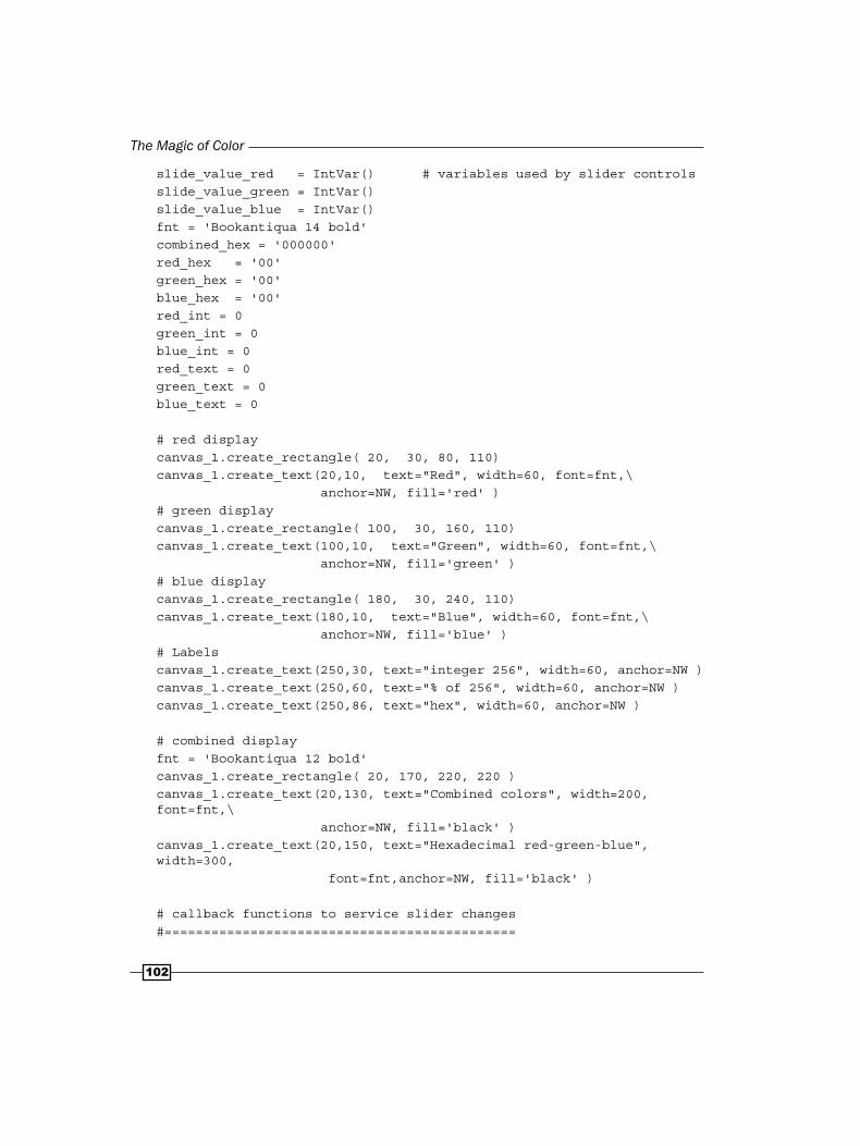
The Magic of Color
102
slide_value_red = IntVar() # variables used by slider controlsslide_value_green = IntVar()slide_value_blue = IntVar()fnt = 'Bookantiqua 14 bold'combined_hex = '000000'red_hex = '00'green_hex = '00'blue_hex = '00'red_int = 0green_int = 0blue_int = 0red_text = 0green_text = 0blue_text = 0
# red displaycanvas_1.create_rectangle( 20, 30, 80, 110)canvas_1.create_text(20,10, text="Red", width=60, font=fnt,\ anchor=NW, fill='red' )# green displaycanvas_1.create_rectangle( 100, 30, 160, 110)canvas_1.create_text(100,10, text="Green", width=60, font=fnt,\ anchor=NW, fill='green' )# blue displaycanvas_1.create_rectangle( 180, 30, 240, 110)canvas_1.create_text(180,10, text="Blue", width=60, font=fnt,\ anchor=NW, fill='blue' )# Labelscanvas_1.create_text(250,30, text="integer 256", width=60, anchor=NW )canvas_1.create_text(250,60, text="% of 256", width=60, anchor=NW )canvas_1.create_text(250,86, text="hex", width=60, anchor=NW )
# combined displayfnt = 'Bookantiqua 12 bold'canvas_1.create_rectangle( 20, 170, 220, 220 )canvas_1.create_text(20,130, text="Combined colors", width=200, font=fnt,\ anchor=NW, fill='black' )canvas_1.create_text(20,150, text="Hexadecimal red-green-blue", width=300, font=fnt,anchor=NW, fill='black' )
# callback functions to service slider changes#=============================================
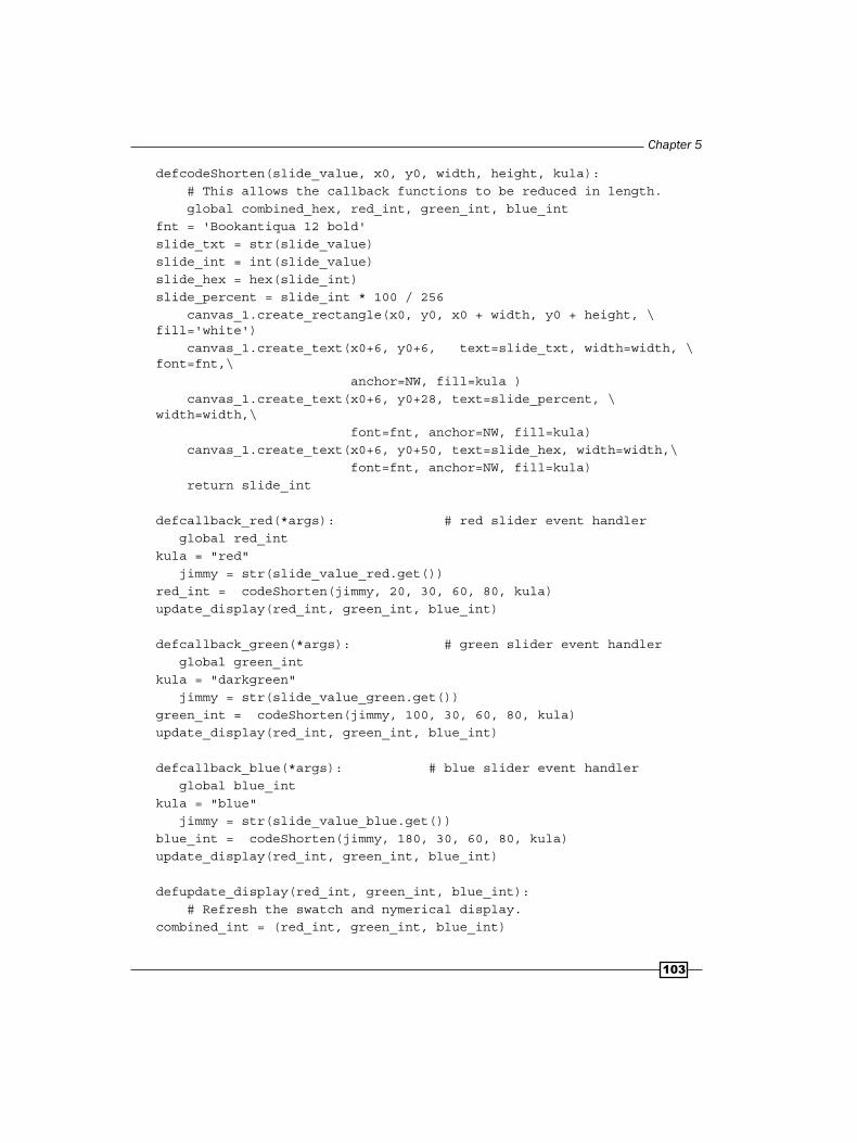
Chapter 5
103
defcodeShorten(slide_value, x0, y0, width, height, kula): # This allows the callback functions to be reduced in length. global combined_hex, red_int, green_int, blue_intfnt = 'Bookantiqua 12 bold'slide_txt = str(slide_value)slide_int = int(slide_value)slide_hex = hex(slide_int)slide_percent = slide_int * 100 / 256 canvas_1.create_rectangle(x0, y0, x0 + width, y0 + height, \ fill='white') canvas_1.create_text(x0+6, y0+6, text=slide_txt, width=width, \ font=fnt,\ anchor=NW, fill=kula ) canvas_1.create_text(x0+6, y0+28, text=slide_percent, \ width=width,\ font=fnt, anchor=NW, fill=kula) canvas_1.create_text(x0+6, y0+50, text=slide_hex, width=width,\ font=fnt, anchor=NW, fill=kula) return slide_int
defcallback_red(*args): # red slider event handler global red_intkula = "red" jimmy = str(slide_value_red.get())red_int = codeShorten(jimmy, 20, 30, 60, 80, kula)update_display(red_int, green_int, blue_int)
defcallback_green(*args): # green slider event handler global green_intkula = "darkgreen" jimmy = str(slide_value_green.get())green_int = codeShorten(jimmy, 100, 30, 60, 80, kula)update_display(red_int, green_int, blue_int)
defcallback_blue(*args): # blue slider event handler global blue_intkula = "blue" jimmy = str(slide_value_blue.get())blue_int = codeShorten(jimmy, 180, 30, 60, 80, kula)update_display(red_int, green_int, blue_int)
defupdate_display(red_int, green_int, blue_int): # Refresh the swatch and nymerical display.combined_int = (red_int, green_int, blue_int)

The Magic of Color
104
combined_hex = '#%02x%02x%02x' % combined_int canvas_1.create_rectangle( 20, 170, 220 , 220, fill='white') canvas_1.create_text(26, 170, text=combined_hex, width=200,\ anchor=NW, font='Bookantiqua 16 bold') canvas_1.create_rectangle( 0, 400, 300, 230, fill=combined_hex)
slide_value_red.trace_variable("w", callback_red)slide_value_green.trace_variable("w", callback_green)slide_value_blue.trace_variable("w", callback_blue)
slider_red = Scale(root, # red slider specification # parameters. length = 400,fg = 'red',activebackground = "tomato", background = "grey",troughcolor = "red", label = "RED", from_ = 0, to = 255, resolution = 1, variable = slide_value_red, orient = 'vertical')
slider_red.grid(row=0, column=2)
slider_green =Scale(root, # green slider specification # parameters. length = 400,fg = 'dark green',activebackground = "green yellow", background = "grey",troughcolor = "green", label = "GREEN", from_ = 0, to = 255, resolution = 1, variable = slide_value_green, orient = 'vertical')
slider_green.grid(row=0, column=3)
slider_blue = Scale(root, # blue slider specification # parameters.

Chapter 5
105
length = 400,fg = 'blue',activebackground = "turquoise", background = "grey",troughcolor = "blue", label = "BLUE", from_ = 0, to = 255, resolution = 1, variable = slide_value_blue, orient = 'vertical')
slider_blue.grid(row=0, column=4)
root.mainloop()
How it works...Red, green, and blue color values ranging from zero (no color at all) to 255 (full saturated primary color) are set by the position of a slider widget that is self explanatory to use. Every time a slider is moved, the values from all three sliders are combined and displayed graphically on a color swatch as well as numerically. There is no better way of explaining the relationships between primary color components expressed as 0 to 255 integer values, hexadecimal values, and pure or combined colors.
There's more...This widget has the swatch placed at the edge of the bottom-left corner to let you drag it close to an area of a picture underneath in order to be able to match the color visually and read off its hex value. There is also a separate window filled with color that can be moved freely around the screen. If you wanted to match a color to some portion of an image in a photo, you could place this swatch right next to the patch of interest in the image and move the sliders until you achieve a decent match and then note the hex value.
There are other tools to select colorsThe last example in this chapter demonstrates color mixers built in Python modules.
Is there a way to make neater slide controllers?The use of slider widgets as a graphical method of entering numbers which need to share screen real estate with our canvas is sometimes inconvenient. Why can't we make our number controllers just another kind of drawn object inside our canvas? Can we make the slide controllers smaller, neater, and less obtrusive? The answer is yes and we explore this idea in Chapter 7, Combining Raster and Vector Pictures.

The Magic of Color
106
The animated graded color wheelWe draw a smoothly-graded version of the artists color mixing wheel and animate it to allow the viewer to watch how the rgb hex color value changes as the blended color spectrum is being drawn.
How to do it...Copy, save, and run this example as you have done with previous ones and watch the spectrum unfold numerically and colorfully. The following screenshot shows a graded color wheel.
#animated_color_wheel_1.py# >>>>>>>>>>>>>>>>>>>>>>>from Tkinter import *root = Tk()root.title("Animated Color Wheel")
cw = 300 # canvas widthch = 300 # canvas heightcanvas_1 = Canvas(root, width=cw, height=ch, background="black")canvas_1.grid(row=0, column=1) cycle_period = 200

Chapter 5
10�
redFl = 255.0greenFl = 0blueFl = 0kula = "#000000"
arcStart = 89arcEnd = 90
xCentr = 150yCentr = 160radius = 130circ = xCentr - radius, yCentr + radius, xCentr + radius, yCentr - \ radius
# angular position markers, degreesA_ANG = 0B_ANG = 60C_ANG = 120D_ANG = 180E_ANG = 240F_ANG = 300#G_ANG = 1G_ANG = 359intervals = 60 # degrees
# Percent color at each position marker# index 0 1 2 3 4 5 6 7redShift = 100, 100, 0, 0, 0, 100, 100 # percent of redgreenShift = 0, 100, 100, 100, 0, 0, 0 # percent of greenblueShift = 0, 0, 0, 100, 100, 100, 0 # percent of blue
# Rate of change of color per degree, rgb integer counts per degree.red_rate = [0,1,2,3,4,5,6,7]green_rate = [0,1,2,3,4,5,6,7]blue_rate = [0,1,2,3,4,5,6,7]
# Calibrate counts-per-degree in each interval, place in xrate listfor i in range(0,6):red_rate[i] = 256.0 * (redShift[i+1] - redShift[i])/(100 * \ intervals)green_rate[i] = 256.0 * (greenShift[i+1] - greenShift[i])/(100 * \ intervals)blue_rate[i] = 256.0 * (blueShift[i+1] - blueShift[i])/(100 * \ intervals)

The Magic of Color
10�
def rgb2hex(redFl, greenFl, blueFl): # Convert integer to hex color. red = int(redFl) green = int(greenFl) blue = int(blueFl)rgb = red, green, blue return '#%02x%02x%02x' % rgb
for i in range (0, 359): canvas_1.create_arc(circ, start=arcStart, extent=arcStart - arcEnd,\ fill= kula, outline= kula)arcStart = arcEndarcEnd -=1
# Color component transitions in 60 degree sectors if i>A_ANG and i<B_ANG:redFl += red_rate[0]greenFl += green_rate[0] blueFl += blue_rate[0]kula = rgb2hex(redFl, greenFl, blueFl)
if i>B_ANG and i<C_ANG:redFl += red_rate[1]greenFl += green_rate[1] blueFl += blue_rate[1]kula = rgb2hex(redFl, greenFl, blueFl)
if i>C_ANG and i<D_ANG:redFl += red_rate[2]greenFl += green_rate[2] blueFl += blue_rate[2]kula = rgb2hex(redFl, greenFl, blueFl)
if i>D_ANG and i<E_ANG:redFl += red_rate[3]greenFl += green_rate[3] blueFl += blue_rate[3]kula = rgb2hex(redFl, greenFl, blueFl)

Chapter 5
10�
if i>E_ANG and i<F_ANG:redFl += red_rate[4]greenFl += green_rate[4] blueFl += blue_rate[4]kula = rgb2hex(redFl, greenFl, blueFl)
if i>F_ANG and i<G_ANG:redFl += red_rate[5]greenFl += green_rate[5] blueFl += blue_rate[5]kula = rgb2hex(redFl, greenFl, blueFl)
#kula = rgb2hex(redFl, greenFl, blueFl) canvas_1.create_text(100, 20, text=kula, fill='white', \ width=200,\ font='SansSerif 12 ', tag= 'degreesAround', anchor= SW) canvas_1.update() # This refreshes the # drawing on the canvas. canvas_1.after(cycle_period) # This makes execution pause for # 200 milliseconds. canvas_1.delete('degreesAround') # This erases the # changing text
root.mainloop()
How it works...The coding ideas used here are relatively simple. In essence, we have the executing code work through the process of drawing a colored arc from zero to 358 degrees. At each thin slice of the wedge red, green, and blue components are added according to calculations of linearly increasing or decreasing ramp values redFL, greenfly, and blueFL in counts-per-degree. By ramp, we mean a gradually increasing value from zero to 100%. The ramp values are controlled by transition points (A_ANG, B_ANG, and so on) evenly spaced at 60 degree intervals around the periphery of the colored disk.
The rgb2hex(red, green, blue) function converts the red, green, and blue floating point values into the form of a hexadecimal number that Tkinter will interpret as a color. For the viewer's edification, this number is displayed at the top of the canvas.

The Magic of Color
110
Tkinter's own color picker-mixerTkinter has its own color chooser tool that is remarkably simple to use.
Four lines of code gets you a tool of elegance and usefulness.
How to do it...Copy, save, and run this example as you have done with previous programs. The following screenshot shows the Tkinter's color picker (MS windows XP).
The following screenshot shows the Tkinter's color picker (Linux – Ubuntu 9.10).
# color_picker_1 .py#>>>>>>>>>>>>>>>from Tkinter import *from tkColorChooser import askcolor
askcolor()mainloop()
Dow
nlo
ad fro
m W
ow
! eBook
<w
ww
.wow
ebook.
com
>

Chapter 5
111
How it works...This tool is so remarkably easy to use you will ask why we have bothered with the more cumbersome versions shown in the numerical color mixing-matching palette example. There are two reasons. Firstly we can see how to manipulate color inside python code. And secondly, the independent swatch window that you can move around on top of pictures can be useful.
There's more...The subject of color mixing, nomenclature and tasteful color combinations is vast and interesting. The web provides some excellent sites explaining this art and science very elegantly.
Here is a selection of some of the best webpages that explain the ideas well.
http://www.1728.com/colors.htm: A display of over 400 html-recognizable named color swatches with their hex equivalents, arranged in alphabetic order. The color swatches displayed are large so you can see the subtle differences between similar colors.http://aggie-horticulture.tamu.edu/floriculture/container-garden/lesson/colorwheel.html: A flower color wheel using names of colors that florists use.
http://realcolorwheel.com/tubecolors.htm: An artist's color wheel, where the colors are matched up to the names of tube pigments that an artist would purchase from an art supply shop.
http://www.colormatters.com/colortheory.html: Elegantly simplified color combination practice, with rich sources of backup and complimentary information. This has loads of illustrations and examples.http://en.wikipedia.org/wiki/Web_colors
The article titled "web colors" in Wikipedia, the free encyclopedia.
http://colorschemedesigner.com/: This website is a most magnificent and complete treatise on the art and science of color. It has everything. Play with the tools here for 15 minutes and you will learn just about everything you will ever need regarding the mixing of colors and how colors can be combined tastefully. This site is the best of the best.


6Working with Pictures
In this chapter, we will cover:
Picture formats in native Python
Opening an image and discovering its attributes
The Python image Library format conversions: .jpg, .png, .tiff, .gif, and, .bmp
Image rotation in the plane
Re-sizing images
Re-sizing with correct aspect ratio
Rotating images
Separating color bands
Red, green, and blue color re-mixing
Combining images by blending
Blending images by varying percentages
Making composites with image masks
Offset (roll) an image horizontally and vertically
Geometric transformations: horizontal and vertical flipping and rotation
Filters: sharpen, blur, edge enhance, emboss, smooth, contour, and detail
Apparent rotation by re-sizing
Now we will work with raster images. These are things like photographs, bitmap images, and digital paintings – all the image types that are NOT the vector graphic drawings we have been using until now. Raster images are made up of pixels, which is short for picture elements. Vector images are defined and processed as mathematical shape and color expressions that can be altered by algebra and arithmetic directly under your control. These vector graphics are only one part of the computer graphics world.

Working with Pictures
114
The other part is concerned with the representation and manipulation of photographic images and painted bitmap images, generally referred to as raster images. The only raster image type that Python recognizes are GIF (Graphics Interchange Format) images which have a limited range of color capability – GIF can work with 256 different colors as opposed to 16.7 million with .png or .jpg. The advantage is that GIF image control in Python allows you to animate them, but basic Tkinter provides no library of functions that can manipulate and alter raster images.
However, there is a very useful bundle of Python modules, the Python Imaging Library (PIL), which is designed just for raster image manipulation. It has most of the basic functions that good photo editing tools have. Modules in the PIL easily convert from one format to another including GIF, PNG, TIFF, JPEG, BMP. and PIL will work with many others, but the ones mentioned previously are probably the most common ones. The Python Image Library is an important part of your general graphics tool kit and skills repertoire.
To reduce confusion, we shall use the file extension abbreviations, like .gif, .png, .jpg and so on as the name of file formats like GIF, PNG, and JPEG.
Opening an image file and discovering its attributes
First we need to test if the PIL is loaded into the library where the rest of our Python modules are. The simplest way to test this is to try and open a file using the image_open() function of the Image module.
Getting readyIf the Python Imaging Library (PIL) is not already installed on our file system, and is ready and accessible to Python, we will need to find and install it. Tkinter is not needed for raster image processing. You will note that there are no from Tkinter import * and no root = tK() or root.mainloop() statements.
You can download PIL from http://www.pythonware.com/products/pil/
This site contains source code, MS Windows installation executables, and handbooks in either HTML or PDF formats.
One of the best explanatory documents on PIL is a PDF file at New Mexico Tech Computer Center http:// infohost.nmt.edu/tcc/help/pubs/pil.pdf. It is clear and concise.

Chapter 6
115
In all the examples that follow in this chapter, all images that get saved to our hard drive are placed into a folder called picsx inside the folder constr. This is to keep the results separate from the pics1 folder which contains all the input images that will be used. This saves us from the dilemma of deciding what to keep and what to throw away. You should keep everything in pics1 and can discard anything in picsx as it should be simple to re-run the programs that created those files.
How to do it...Copy the following code into an editor and save it as image_getattributes_1.py and then execute as with all previous programs. In this program, we are going to use the PIL to discover the attributes of a JPG format image. Remember that although Python on its own only recognizes GIF images, the PIL module can work with many image formats. Until we can get this tiny program to work we can go no further using PIL.
# image_getattributes_1.py# >>>>>>>>>>>>>>>>>>import ImageimageFile = "/constr/pics1/canary_a.jpg"
im_1 = Image.open(imageFile)im_width = im_1.size[0]im_height = im_1.size[1]im_mode = im_1.modeim_format = im_1.formatprint "Size: ",im_width, im_heightprint "Mode: ",im_modeprint "Format: ",im_formatim_1.show()
How it works...The Image module, which is part of the PIL library, has a method Image_open() which opens files that are recognizable as image files. It does not display the images. This may be confusing. Opening a file means that our application program has found where the file is located and has dealt with all the permissions and administration required for loading the file. When you open a file, the file header is read to determine the file format and extract things like mode, size, and, other properties required to decode the file, but the rest of the file is not processed until later. Mode is a term used to refer to the way the data bytes containing the image are to be interpreted – whether a particular byte refers to the red channel or the transparency channel and so on. Only when the Image module gets commands to view the file, change its size, view one of the color channels, rotate it, or any of the dozens of things that the modules in PIL can do to image files, will it actually be loaded from the hard drive and into memory.

Working with Pictures
116
If we want to view the image, then we use the im_1. show() method. Just add the line im.show() at the end.
Why do we need to get image attributes? When we are going to change and manipulate images, we need to make changes to the attributes and therefore we often need to be able to find out what they are originally.
There's more...The Image module of PIL (the Python Imaging Library) can read and write (open and save) the common image formats. The following formats can be both read and written: BMP, GIF, IM, JPG, JPEG, JPE, PCX, PNG, PBM, PPN, TIF, TIFF, XBM, XPM.
The following file formats can only be read: PCD, DCX, PSD. If we needed to store image files which were PCD, DCX, or PSD, then we would first convert them into one of the file formats that did work like PNG, TIFF, JPEG, or BMP. Python on its own, without the PIL module, only deals with GIF files so these would be preferred file formats for self-contained applications. JPG files are ubiquitous and therefore we need to prove that the code we write can use JPG, GIF, PNG, and, BMP formats.
Things we need to know about image formatsIt is useful to know the following about file image formats:
GIF image files are the smallest and fastest to use and transport down a wire. They are probably the best balance of image quality and file size. On the downside, they have a limited range of colors and are not good for high quality pictures.
JPEG images are the most common ones on the web. The quality can vary from high to low depending on what degree of compression you specify. A large image can be compressed substantially, but you will lose image quality.
TIFF images are large and high quality/resolution. Detailed engineering drawings are often archived as TIFF files.
PNG images are a modern high quality replacement for GIF files. But Tkinter will not recognize them.
BMP images are uncompressed and a bit old fashioned but there are still many around. Not recommended.
When working with images in PIL, PNG images are a convenient form to use. However, if you are preparing images for display inside Python programs on the widest variety of platforms, then you need to convert them into GIF format before saving them.

Chapter 6
11�
Images and the numbers gameImage formats are like studying ancient languages – the more you learn, the more complicated things get. But here are the basic numbers governing them that give you some insight.
GIF has a maximum of 256 colors, but can use a lot less.
PNG has a maximum of about 14000, different colors.
JPEG can handle 16 million – the same number of colors as the #rrggbb numbers used in the previous chapter.
Most images from digital cameras are compressed into JPG images and this reduces the range of colors. Therefore, in most cases, we can convert them to PNG images without apparent loss of quality.
Open, view, and save an image in a different file format
Quite often, there is some image we want to work with but it is in the wrong format. Most web images are JPEG (.jpg) files. Native Python will only recognize GIF (.gif) formats.
Getting readyGet hold of a .jpg image file and save or copy it into a directory you have created for this imaging work. For the purpose of these exercises we are going to assume there is a directory named constr (abbreviation for "construction site"). In the code, you will see images addressed in the form /constr/pics1/images-name.ext. image-name.ext is the actual image you have selected to work with. This means that the Python program expects to find the file you are asking it to open, inside a system directory called constr. You can change this to wherever you decide is the best place for you to make a mess in – like an artist's studio. The path to retrieve your image file can even be a web address.
So for this example, there is an image named duzi_leo_1.jpg, a JPEG image stored inside a folder (directory) called pics1 which in turn is inside constr.
How to do it...Execute the program shown as follows in the usual fashion.
# images_jpg2png_1.py#>>>>>>>>>>>>>>>>>>>>>>>>>>>>>>>>>>>>>>>>import Imageim_1 = Image.open("/constr/pics1/duzi_leo_1.jpg")im_1.show()im_1.save('/constr/picsx/duzi_leo_2.png', 'PNG')

Working with Pictures
11�
How it works...In the typical Python fashion the designers of Python have made things as simple as they possibly could for the coder. What happens here is that we create an instance im_1 of an image object which is in JPEG format (extension .jpg) and we command that it be saved as PNG (extension .png). The complex conversion takes place out of sight. We display the image to reassure ourselves that it has been found.
Finally we convert it to PNG format and save it as duzi_leo_2.png.
There's more...We would like to know that we can convert any image format to any other format. Unfortunately image formats are something of a tower of Babel phenomenon. For reasons of history, technology evolution, patent restrictions, and proprietary commercial hegemony many image formats were not intended to be openly readable. For instance up until 2004, GIF was proprietary. PNG was developed as an alternative. The next example presents code for discovering which conversions will work on your platform.
Image format conversion for JPEG, PNG, TIFF, GIF, BMP
We start with a PNG format image then save it in each of the following formats: JPG, PNG, GIF, TIFF, and BMP and save them on the local hard drive. Then we take the saved image formats and convert each in turn into the other formats. Thus we test all the likely conversion combinations.
Getting readyWe need to place a JPG image into the folder /constr/pics1. A specific PNG image design to emphasize flaws in the different formats is provided with the name test_pattern_a.png.
How to do it...Execute the program shown as before. Read their describing 'metadata' on the command terminal

Chapter 6
11�
# images_one2another_1.py#>>>>>>>>>>>>>>>>>>>>>import Image
# Convert a jpg image to OTHER formatsim_1 = Image.open("/constr/pics1/test_pattern_1.jpg")im_1.save('/constr/picsx/test_pattern_2.png', 'PNG')im_1.save('/constr/picsx/test_pattern_3.gif', 'GIF')im_1.save('/constr/picsx/test_pattern_4.tif', 'TIFF')im_1.save('/constr/picsx/test_pattern_5.bmp', 'BMP')
# Convert a png image to OTHER formatsim_2 = Image.open("/constr/picsx/test_pattern_2.png")im_2.save('/constr/picsx/test_pattern_6.jpg', 'JPEG')im_2.save('/constr/picsx/test_pattern_7.gif', 'GIF')im_2.save('/constr/picsx/test_pattern_8.tif', 'TIFF')im_2.save('/constr/picsx/test_pattern_9.bmp', 'BMP')
# Convert a gif image to OTHER formats# It seems that gif->jpg does not workim_3 = Image.open("/constr/pics1/test_pattern_3.gif")#im_3.save('/constr/pics1/test_pattern_10.jpg', 'JPEG')# "IOError "cannot write mode P as JPEG"im_3.save('/constr/picsx/test_pattern_11.png', 'PNG')im_3.save('/constr/picsx/test_pattern_12.tif', 'TIFF')im_3.save('/constr/picsx/test_pattern_13.bmp', 'BMP')
# Convert a tif image to OTHER formatsim_4 = Image.open("/constr/picsx/test_pattern_4.tif")im_4.save('/constr/picsx/test_pattern_14.png', 'PNG')im_4.save('/constr/picsx/test_pattern_15.gif', 'GIF')im_4.save('/constr/picsx/test_pattern_16.tif', 'TIFF')im_4.save('/constr/picsx/test_pattern_17.bmp', 'BMP')

Working with Pictures
120
# Convert a bmp image to OTHER formatsim_5 = Image.open("/constr/picsx/test_pattern_5.bmp")im_5.save('/constr/picsx/test_pattern_18.png', 'PNG')im_5.save('/constr/picsx/test_pattern_19.gif', 'GIF')im_5.save('/constr/picsx/test_pattern_20.tif', 'TIFF')im_5.save('/constr/picsx/test_pattern_21.jpg', 'JPEG')
How it works...This conversion just works if PIL is installed. One exception is that conversions from GIF to JPG will not work. It is interesting to have the contents of the folder /constr/pics1 already open prior to executing the program and watch the images successively appear as the execution takes pace.
There's more...Note that it is difficult to notice loss of image quality for any of the image qualities except for GIF images. The problems are most noticeable when the GIF conversion algorithm has to make a choice between two similar colors as shown in the figure.
Does size count?The original test_pattern_1.jpg was 77 kilobytes. All the images derived from it were four to ten times larger, even the low quality GIF images. The reason is that only the JPG and GIF images are lossy, meaning that some image information is discarded in the conversion and it can't be recovered.
Image rotation in the plane of the imageWe have an image lying on its side and we need to fix it up by rotating it clockwise by 90 degrees. We want a stored copy of the corrected image.
Getting readyWe need to place a PNG image into the folder /constr/pics1. In the following code, we have used the image dusi_leo.png. This image has prominent red and yellow components.

Chapter 6
121
How to do it...Execute the program shown as before.
# image_rotate_1.py#>>>>>>>>>>>>>>>>import Imageim_1 = Image.open("/constr/pics1/dusi_leo.png")im_2= im_1.rotate(-90)im_2.show()im_2.save("/constr/picsx/dusi_leo_rightway.png")
How it works...The displayed image will be correctly oriented. Note that we can rotate the image by amounts as small as one degree, but no smaller than that. There are other transformations that can rotate an image to integer multiples of 90 degrees. These are demonstrated under the title Multiple Transformations.
There's more...How would we create the effect of a smoothly rotating image? Attempting it with PIL on its own does not work. PIL is designed to do the calculation intensive operations for manipulating and transforming images. It is not possible to display one image after another in a time-controlled sequence. For this, you would need Tkinter and Tkinter will only work with GIF images.
What we would do would be to first create a series of images, each slightly more rotated than the previous one and store each image. Later, we would run a Python Tkinter program that displayed the series of images in a time-controlled sequence. This would animate the rotation. There are difficulties related to the fact that the rotated images must be placed in a frame that has the same size and orientation as the original image. These kinds of problems are tackled in the next chapter. Some surprisingly effective results can be achieved.
Image size alterationWe reduce the size of a large image file (1.8 megabytes) down to 24.7 kilobytes. But the image gets distorted because the height-to-width ratio is not taken into account.
Getting readyAs we did for the previous recipe, we need to place the dusi_leo.png image into the folder /constr/pics1.
Dow
nlo
ad fro
m W
ow
! eBook
<w
ww
.wow
ebook.
com
>

Working with Pictures
122
How to do it...To change the size of an image we need to specify the final dimensions as well as specify a filter type that provides rules for filling in any pixel gaps that result from the re-sizing process. Execute the program shown as before. The following image shows the result.
# image_resize_1.py#>>>>>>>>>>>>>>>>import Imageim_1 = Image.open("/constr/pics1/dusi_leo_1.jpg")
# adjust width and height to desired sizewidth = 300height = 300# NEAREST Filter is compulsory to resize the imageim_2 = im_1.resize((width, height), Image.NEAREST)
im_2.save("/constr/picsx/dusi_leo_2.jpg")
How it works...Here we changed the size of a picture to fit a 300x300 pixel rectangle. If the image is increased in size, extra pixels need to be added. If the image is reduced, then pixels have to be discarded. Which particular pixels are added, what color they will be has to be decided automatically by an algorithm in the re-sizing method. There are several ways provided in PIL to do this. These pixel-adding algorithms are made available as filters.
This is what filters are designed for and in the preceding example we have chosen to use the nearest filter. This is documented as using the value of the NEAREST neighboring pixel. The documentation is a bit ambiguous because it does not explain which nearest pixel will be selected. In a rectangular grid, the pixels to the north, south, east, and west are equally close. Other possible filters to use are BILINEAR (linear interpolation in a 2x2 environment), BICUBIC (cubic spline interpolation in a 4x4 environment), or ANTIALIAS (a high-quality down-sampling filter).
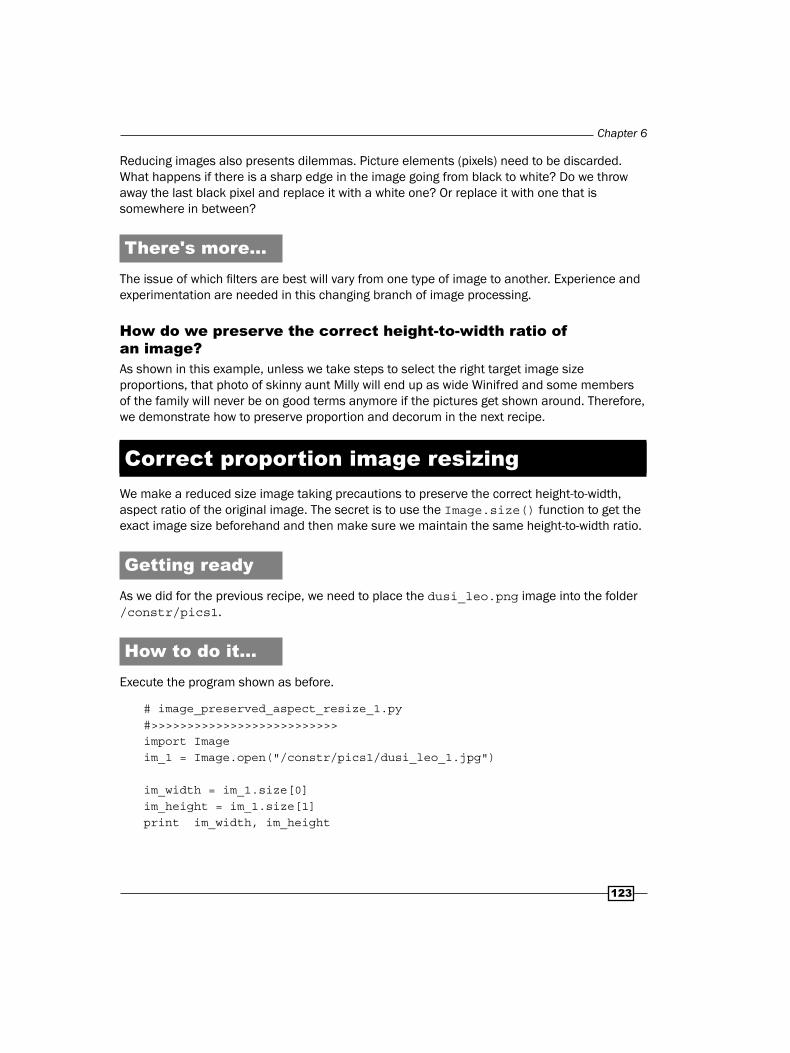
Chapter 6
123
Reducing images also presents dilemmas. Picture elements (pixels) need to be discarded. What happens if there is a sharp edge in the image going from black to white? Do we throw away the last black pixel and replace it with a white one? Or replace it with one that is somewhere in between?
There's more...The issue of which filters are best will vary from one type of image to another. Experience and experimentation are needed in this changing branch of image processing.
How do we preserve the correct height-to-width ratio of an image?As shown in this example, unless we take steps to select the right target image size proportions, that photo of skinny aunt Milly will end up as wide Winifred and some members of the family will never be on good terms anymore if the pictures get shown around. Therefore, we demonstrate how to preserve proportion and decorum in the next recipe.
Correct proportion image resizingWe make a reduced size image taking precautions to preserve the correct height-to-width, aspect ratio of the original image. The secret is to use the Image.size() function to get the exact image size beforehand and then make sure we maintain the same height-to-width ratio.
Getting readyAs we did for the previous recipe, we need to place the dusi_leo.png image into the folder /constr/pics1.
How to do it...Execute the program shown as before.
# image_preserved_aspect_resize_1.py#>>>>>>>>>>>>>>>>>>>>>>>>>>import Imageim_1 = Image.open("/constr/pics1/dusi_leo_1.jpg")
im_width = im_1.size[0]im_height = im_1.size[1]print im_width, im_height

Working with Pictures
124
new_size = 0.2 # New image to be reduced to one fifth of original.# adjust width and height to desired sizewidth = int(im_width * new_size)height = int(im_height * new_size)# Filter is compulsory to resize the imageim_2 = im_1.resize((width, height), Image.NEAREST)
im_2.save("/constr/picsx/dusi_leo_3.jpg")
How it works...The Image.size() function returns two integers, - the width, size[0], and height, size[1] of the opened image. We use the scaling multiplier new_size to scale both the width and the height by the same proportion.
Separating one color band in an imageWe isolate just the green portion or band of an image.
Getting readyAs we did for the previous recipe, we need to place the dusi_leo.png image into the folder /constr/pics1.
How to do it...Execute the program shown as before.
#image_get_green_1.py#>>>>>>>>>>>>>>>>>>import ImageEnhanceimport Image
red_frac = 1.0green_frac = 1.0blue_frac = 1.0
im_1 = Image.open("/a_constr/pics1/dusi_leo_1.jpg")
# split the image into individual bandssource = im_1.split()R, G, B = 0, 1, 2
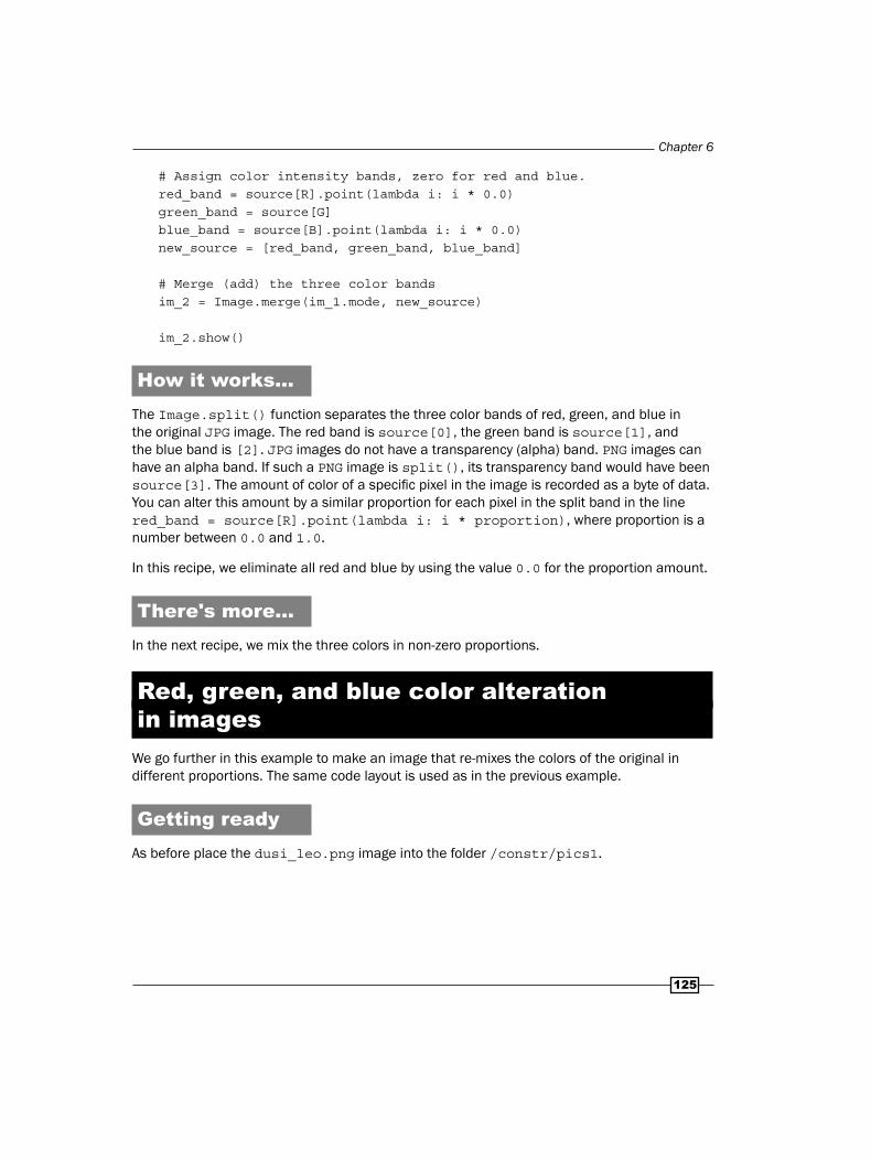
Chapter 6
125
# Assign color intensity bands, zero for red and blue.red_band = source[R].point(lambda i: i * 0.0)green_band = source[G]blue_band = source[B].point(lambda i: i * 0.0)new_source = [red_band, green_band, blue_band]
# Merge (add) the three color bandsim_2 = Image.merge(im_1.mode, new_source)
im_2.show()
How it works...The Image.split() function separates the three color bands of red, green, and blue in the original JPG image. The red band is source[0], the green band is source[1], and the blue band is [2]. JPG images do not have a transparency (alpha) band. PNG images can have an alpha band. If such a PNG image is split(), its transparency band would have been source[3]. The amount of color of a specific pixel in the image is recorded as a byte of data. You can alter this amount by a similar proportion for each pixel in the split band in the line red_band = source[R].point(lambda i: i * proportion), where proportion is a number between 0.0 and 1.0.
In this recipe, we eliminate all red and blue by using the value 0.0 for the proportion amount.
There's more...In the next recipe, we mix the three colors in non-zero proportions.
Red, green, and blue color alteration in images
We go further in this example to make an image that re-mixes the colors of the original in different proportions. The same code layout is used as in the previous example.
Getting readyAs before place the dusi_leo.png image into the folder /constr/pics1.

Working with Pictures
126
How to do it...Execute the following code.
#image_color_manip_1.py#>>>>>>>>>>>>>>>>>>>>>>>>>>>>>>>>>>>>>>>>import ImageEnhance, Imageim_1 = Image.open("/constr/pics1/dusi_leo_smlr_1.jpg")
# Split the image into individual bandssource = im_1.split()
R, G, B = 0, 1, 2# Select regions where red is less than 100red_band = source[R]green_band = source[G]blue_band = source[B]
# Process the red band: intensify red x 2out_red = source[R].point(lambda i: i * 2.0)
# Process the green band: weaken by 20%out_green = source[G].point(lambda i: i * 0.8)
# process the blue band: Eliminate all blueout_blue = source[B].point(lambda i: i * 0.0)
# Make a new source of color band valuesnew_source = [out_red, out_green, out_blue]
# Add the three altered bands back togetherim_2 = Image.merge(im_1.mode, new_source)im_2.show()
How it works...As before, the Image.split() function separates the three color bands of red, green, and blue from the original JPG image. In this case, the amounts of each red, green, and blue are 200%, 20%, and 0% of blue respectively.

Chapter 6
12�
There's more...Altering the proportion of colors in existing pictures is a complex and subtle art and as we did in the previous chapters, in the next example we provide a recipe that uses slide controls to allow the user to use trial and error to achieve a desirable color mix on a band-separated image.
Slider controlled color manipulationWe construct a tool for the purpose of obtaining a desirable color mix on a band-separated image. The slide control, which we have used previously, is a convenient device for consciously adjusting the relative proportions of color in each primary color band.
Getting readyUse the dusi_leo.png image from the folder /constr/pics1.
How to do it...Execute the following program.
#image_color_adjuster_1.py#>>>>>>>>>>>>>>>>>>>import ImageEnhanceimport Imageimport Tkinterroot =Tkinter.Tk()root.title("Photo Image Color Adjuster")
red_frac = 1.0green_frac = 1.0blue_frac = 1.0
slide_value_red = Tkinter.IntVar()slide_value_green = Tkinter.IntVar()slide_value_blue = Tkinter.IntVar()
im_1 = Image.open("/constr/pics1/dusi_leo_smlr_1.jpg")im_1.show()source = im_1.split() # split the image into individual bandsR, G, B = 0, 1, 2

Working with Pictures
12�
# Assign color intensity bandsred_band = source[R]green_band = source[G]blue_band = source[B]#===============================================# Slider and Button event service functions (callbacks)def callback_button_1(): # Adjust red intensity by slider value. out_red = source[R].point(lambda i: i * red_frac) out_green = source[G].point(lambda i: i * green_frac) # Adjust # green out_blue = source[B].point(lambda i: i * blue_frac) # Adjust # blue new_source = [out_red, out_green, out_blue] im_2 = Image.merge(im_1.mode, new_source) # Re-combine bands im_2.show()
button_1= Tkinter.Button(root,bg= "sky blue", text= "Display adjusted image \ (delete previous one)", command=callback_ \button_1)button_1.grid(row=1, column=2, columnspan=3)
def callback_red(*args): global red_frac red_frac = slide_value_red.get()/100.0
def callback_green(*args): global green_frac green_frac = slide_value_green.get()/100.0
def callback_blue(*args): global blue_frac blue_frac = slide_value_blue.get()/100.0
slide_value_red.trace_variable("w", callback_red)slide_value_green.trace_variable("w", callback_green)slide_value_blue.trace_variable("w", callback_blue)
slider_red = Tkinter.Scale(root, length = 400, fg = 'red', activebackground = "tomato", background = "grey", troughcolor = "red",

Chapter 6
12�
label = "RED", from_ = 0, to = 200, resolution = 1, variable = slide_value_red, orient = 'vertical')
slider_red.grid(row=0, column=2)
slider_green = Tkinter.Scale(root, length = 400, fg = 'dark green', activebackground = "green yellow", background = "grey", troughcolor = "green", label = "GREEN", from_ = 0, to = 200, resolution = 1, variable = slide_value_green, orient = 'vertical')
slider_green.grid(row=0, column=3)
slider_blue = Tkinter.Scale(root, length = 400, fg = 'blue', activebackground = "turquoise", background = "grey", troughcolor = "blue", label = "BLUE", from_ = 0, to = 200, resolution = 1, variable = slide_value_blue, orient = 'vertical')
slider_blue.grid(row=0, column=4)
root.mainloop()#===============================================
Working with Pictures
130
How it works...Using mouse-controlled slider positions, we adjust the amount of color intensity in each of the red, green, and blue channels. The scale of adjustment goes from zero to 200, but is scaled to a percentage value in the callback functions.
In source = im_1.split(), the split() method separates the image into red, green, and blue bands. The point(lambda i: i * intensity) method multiplies the color value for each pixel in a band by an 'intensity' value and the merge(im_1.mode, new_source) method re-combines the resultant bands into a new image.
In this example PIL and Tkinter are being used together.
If you use from Tkinter import *, you seem to get namespace confusion:
The interpreter says:
" im_1 = Image.open("/a_constr/pics1/redcar.jpg")
AttributeError: class Image has no attribute 'open' ",
but if you just say import Tkinter it seems ok.
But of course now you have to prefix all Tkinter methods with Tkinter.
Combining images by blendingThe effect of blending two images is like projecting two transparent slide images onto a projector screen from two separate projectors where the amount of light from each projector is controlled by proportion setting. The command is of the form Image.blend(image_1, image_2, proportion-of-image_1).
Getting readyUse the two images 100_canary.png and 100_cockcrow.png from the folder /constr/pics1. The 100_ in the titles is a reminder that the images are 100 x 100 pixels in size and we will see the format, size, and type of each image printed onto the console.
How to do it...With the two identical size and mode images in place, execute the following code.
# image_blend_1.py# >>>>>>>>>>>>>>>>import Image

Chapter 6
131
im_1 = Image.open("/constr/pics1/100_canary.png") # mode is RGBAim_2 = Image.open("/constr/pics1/100_cockcrow.png") # mode is RGB
# Check on mode, size and format first for compatibility.print "im_1 format:", im_1.format, ";size:", im_1.size, "; mode:",im_1.modeprint "im_2 format:", im_2.format, ";size:", im_2.size, "; mode:",im_2.modeim_2 = im_2.convert("RGBA") # Make both modes the sameim_4 = Image.blend(im_1, im_2, 0.5)im_4.show()
There's more...From format information, we will see that the mode of the first image is RGBA while the second is RGB. Therefore, it is necessary to first convert the second image to RGBA.
In this particular example, the proportion control was set to 0.5. That is, the two images were blended together by equal amounts. If the proportion setting had been 0.2, then 20% of im_1 would have been combined with 80% of im_2.
More Info Section 1Another way of combining images would be to use a third image as a mask to control the positions where the mask determines both the shape and the proportion of each image in the resulting image.
Blending images by varying percentagesWe blend two images with various amounts of transparency.
How to do it...With the two identical size and mode images in place, execute the following code.
# image_blend_2.py# >>>>>>>>>>>>>>>>>>>>>>>>>>>>>>>>>>>>>>>>>>>>>>>>>>>>>>>import Imageim_1 = Image.open("/constr/pics1/lion_ramp_2.png")im_2 = Image.open("/constr/pics1/fiery_2.png")
# Various degrees of alphaim_3 = Image.blend(im_1, im_2, 0.05) # 95% im_1, 5% im_2im_4 = Image.blend(im_1, im_2, 0.2)

Working with Pictures
132
im_5 = Image.blend(im_1, im_2, 0.5)im_6 = Image.blend(im_1, im_2, 0.6)im_7 = Image.blend(im_1, im_2, 0.8)im_8 = Image.blend(im_1, im_2, 0.95) # 5% im_1, 95% im_2 im_3.save("/constr/picsx/fiery_lion_1.png")im_4.save("/constr/picsx/fiery_lion_2.png")im_5.save("/constr/picsx/fiery_lion_3.png")im_6.save("/constr/picsx/fiery_lion_4.png")im_7.save("/constr/picsx/fiery_lion_5.png")im_8.save("/constr/picsx/fiery_lion_6.png")
How it works...By changing the amount of alpha with which the images are blended, we can control the degree to which each image dominates in the result.
There's more...This kind of process performed on each frame of a movie is the kind of effect often used to fade from one scene to another.
Make a composite image using a mask image
Here, we control the combination of two images using the function Image.composite(image_1, image_2, mask_image).
Getting readyUse the images 100_canary.png, 100_cockcrow.png, and 100_sun_1.png from the folder /constr/pics1. The 100_ in the titles is a reminder that the images are 100 x 100 pixels in size and we will see the format, size, and type of each image printed onto the console.
How to do it...With the three identical size and mode images in place, execute the following code.
# image_composite_1.py# >>>>>>>>>>>>>>>>>import Imageim_1 = Image.open("/constr/pics1/100_canary.png") # mode is RGBA

Chapter 6
133
im_2 = Image.open("/constr/pics1/100_cockcrow.png") # mode is RGBim_3 = Image.open("/constr/pics1/100_sun_1.png")# Check on mode, size and format first for compatibility.print "im_1 format:", im_1.format, ";size:", im_1.size, "; mode:", \im_1.modeprint "im_2 format:", im_2.format, ";size:", im_2.size, "; mode:", \im_2.modeprint "im_3 format:", im_3.format, ";size:", im_3.size, "; mode:", \im_3.mode
im_2 = im_2.convert("RGBA")im_3 = im_3.convert("L")im_4 = Image.composite(im_1, im_2, im_3)
im_4.show()
How it works...From format information, we will see that the mode of the first image is RGBA while the second is RGB. Therefore, it is necessary to first convert the second image to RGBA.
The mask image has to be of the form 1, L, or RGBA and of the same size. In this recipe, we have converted it to mode L which is a 256 value gray-scale image. The value of each pixel in the mask is used to multiply the source images. If the value of a particular pixel in a certain location was 56, then image_1 would be multiplied by 256 – 56 =200 and image_2 would be multiplied by 56.
There's more...There are other effects like Image.eval(function, Image) where each pixel is multiplied by the function and we can convert the function to some complicated algebraic expression. If the image has multiple bands, then the function is applied to each band.
Another effect is the Image.merge(mode, bandList) which creates a multi-band image from multiple single-band images of equal size. We specify the desired mode of the new image. The bandList specifier is a sequence of single-band image components to be combined.
See alsoUsing the image operations shown previously in combinations, there are an endless number of effects that can be achieved. We would be delving into the world of image and signal processing which can get extremely complex and sophisticated. Certain effects have become fairly standard and can be seen in the list of filtering options available in image-processing applications like GIMP and Photoshop.
Dow
nlo
ad fro
m W
ow
! eBook
<w
ww
.wow
ebook.
com
>

Working with Pictures
134
Offset (roll) image horizontally and verticallyWe see here how to roll an image. That is, to shift it to the right or left without losing anything - the image effectively rolls as if the edges were joined. The same process will work in the vertical direction.
Getting readyUse the image canary_a.jpg from the folder /constr/pics1.
How to do it...Execute the following program noting that we need to import a module belonging to PIL called ImageChops. The Chops stands for channel operations.
# image_offset_1.py# >>>>>>>>>>>>>>>import Imageimport ImageChops
im_1 = Image.open("/constr/pics1/canary_a.jpg")
# adjust width and height to desired sizedx = 200dy = 300
im_2 = ImageChops.offset(im_1, dx, dy)im_2.save("/constr/picsx/canary_2.jpg")
How it works...The excellent guide Python Imaging Library by John Shipman written in mid 2009 does not mention ImageChops.
Flip horizontally, vertically, and rotateHere we look at a set of quick and easy transformations that are typical of the operations we would need in a photo viewer.
Getting readyUse the image dusi_leo_1.jpg from the folder /constr/pics1.

Chapter 6
135
How to do it...Execute the following program and see the results in /constr/picsx.
# image_flips_1.py#>>>>>>>>>>>>>>import Imageim_1 = Image.open("/a_constr/pics1/dusi_leo_1.jpg")im_out_1 = im_1.transpose(Image.FLIP_LEFT_RIGHT)im_out_2 = im_1.transpose(Image.FLIP_TOP_BOTTOM)im_out_3 = im_1.transpose(Image.ROTATE_90)im_out_4 = im_1.transpose(Image.ROTATE_180)im_out_5 = im_1.transpose(Image.ROTATE_270)im_out_1.save("/a_constr/picsx/dusi_leo_horizontal.jpg")im_out_1.save("/a_constr/picsx/dusi_leo_vertical.jpg")im_out_1.save("/a_constr/picsx/dusi_leo_90.jpg")im_out_1.save("/a_constr/picsx/dusi_leo_180.jpg")im_out_1.save("/a_constr/picsx/duzi_leo_270.jpg")
How it works...The preceding commands are self-explanatory.
Filter effects: blur, sharpen, contrast, and so on
PIL has an ImageFilter module that has a useful selection of filters for enhancing certain characteristics of images such as sharpening features that were blurred. Ten of these filters are demonstrated in the following recipe.
Getting readyUse the images russian_doll.png from the folder /constr/pics1. Create a folder /constr/picsx for the resulting filtered images. Using a separate folder for the results helps prevent the folder pics1 from becoming overcrowded with a heap of redundant images and work-in-progress. After each execution, we can delete the contents of picsx without the fear of losing source images for the recipes.

Working with Pictures
136
How to do it...Open the folder /constr/picsx on your screen before you execute the following code and watch as the images appear once the execution is complete. The source image was chosen to have a blurred Russian doll on an in-focus background because it allows the effects of the different filters to be readily distinguished.
# image_pileof_filters_1.py# >>>>>>>>>>>>>>>>>>>import ImageFilterim_1 = Image.open("/constr/pics1/russian_doll.png")
im_2 = im_1.filter(ImageFilter.BLUR)im_3 = im_1.filter(ImageFilter.CONTOUR)im_4 = im_1.filter(ImageFilter.DETAIL)im_5 = im_1.filter(ImageFilter.EDGE_ENHANCE)im_6 = im_1.filter(ImageFilter.EDGE_ENHANCE_MORE)im_7 = im_1.filter(ImageFilter.EMBOSS)im_8 = im_1.filter(ImageFilter.FIND_EDGES)im_9 = im_1.filter(ImageFilter.SMOOTH)im_10 = im_1.filter(ImageFilter.SMOOTH_MORE)im_11 = im_1.filter(ImageFilter.SHARPEN)
im_2.save("/constr/picsx/russian_doll_BLUR.png")im_3.save("/constr/picsx/ russian_doll_CONTOUR.png")im_4.save("/constr/picsx/ russian_doll_DETAIL.png")im_5.save("/constr/picsx/ russian_doll_EDGE_ENHANCE.png")im_6.save("/constr/picsx/ russian_doll_EDGE_ENHANCE_MORE.png")im_7.save("/constr/picsx/ russian_doll_EMBOSS.png")im_8.save("/constr/picsx/ russian_doll_FIND_EDGES.png")im_9.save("/constr/picsx/ russian_doll_SMOOTH.png")im_10.save("/constr/picsx/ russian_doll_SMOOTH_MORE.png")im_11.save("/constr/picsx/ russian_doll_SHARPEN.png")
How it works...This recipe shows that the best filtering results are highly dependent on both the feature of the image we wish to enhance or suppress, as well as some subtle characteristics of the individual image being worked on. In the particular example of the Russian doll used here, the EDGE_ENHANCE filter is particularly effective for counteracting the poor focus of the doll. It improves the color contrast in comparison to the SHARPEN filter. Re-size and paste for synthetic rotation

Chapter 6
13�
We want to create an animation that makes an image apparently rotate around a vertical axis in the middle of the picture. In this recipe, we see how the basic sequences of images for the animation are prepared.
We want to make a sequence of images that are progressively narrower – as if they were a poster on a board that was being gradually rotated. Then, we want to paste these narrow images in the middle of a standard-sized black background. If this sequence were displayed as a time-controlled series of frames, we would see the image apparently rotating around a central vertical axis.
Getting readyWe use the image 100_canary.png in a directory /constr/pics1 and we place the results in /constr/picsx to avoid cluttering our source folder /constr/pics1.
How to do it...Again open the folder /constr/picsx on your screen before you execute the following code and watch as the images appear once the execution is complete. This is not necessary but it is interesting to watch the results materialize before your eyes.
# image_rotate_resize_1.py# >>>>>>>>>>>>>>>>>>>>import Imageimport math
THETADEG = 5.0 # degreesTHETARAD = math.radians(THETADEG)
im_1 = Image.open("/constr/pics1/blank.png")im_seed = Image.open("/constr/pics1/100_canary.png") # THE SEED IMAGEim_seq_name = "canary"
#GET IMAGE WIDTH AND HEIGHT - not done here# For the time being assume the image is 100 x 100width = 100height = 100num_images = int(math.pi/(2*THETARAD))Q = []for j in range(0,2*num_images + 1): Q.append(j)

Working with Pictures
13�
for i in range(0, num_images): new_size = width * math.cos(i*THETARAD) # Width for reduced # image im_temp = im_seed.resize((new_size, height), Image.NEAREST) im_width = im_temp.size[0] # Get the width of the reduced image x_start = 50 -im_width/2 # Centralize new image in a 100x100 # square. im_1.paste(im_temp,( x_start,10)) # Paste: This creates the # annoying ghosting. stri = str(i) # Save the reduced image Q[i] = "/constr/picsx/" + im_seq_name + stri + ".gif" im_1.save(Q[i]) # Flip horizontally and save the reduced image. im_transpose = im_temp.transpose(Image.FLIP_LEFT_RIGHT) im_1.paste(im_transpose,( x_start,10)) strj = str(2 * num_images - i) Q[ 2 * num_images - i ] = "/constr/picsx/" + im_seq_name + strj \ + ".gif" im_1.save(Q[ 2 * num_images - i ])
How it works...To mimic the effect of rotation, we reduce the width of each image to cosine(new_angle) where new_angle is increased by 5 degrees of rotation for each image. Then we take this narrowed image and paste it onto a blank black square. Finally we name each picture in the sequence in a systematic way such as canary0.gif, canary1.gif, and so on until the last image is named canary36.gif.
There's more...This example demonstrates the kind of task the Python Imaging Library is well-suited to - when you need to repeatedly perform a controlled transformation on an image or collection of images. The images could be the frames of a video film. Effects like fade-in and fade-out, zoom-out, color-shift, sharpen, and blur are the obvious ones that can be used but your programmer's imagination will be able to come up with many others.

�Combining Raster and
Vector Pictures
In this chapter, we will cover:
Simple animation of a GIF beach ball
The vector walking creature
Bird with shoes walking in the karroo
Making a partially transparent image with Gimp
Diplomat walking at the palace
Spider in the forest
Moving band of images
Continuous band of images
Endless background – a passing cloudscape
Vector graphics as seen in Chapter 2, Drawing Fundamental Shapes and Chapter 3, Handling Text can be shrunk and expanded to any size and in any direction using simple algebra. They can be animated with rotations using basic trigonometry. Raster graphics are limited. They cannot be resized or rotated dynamically while the code is executing. They are more cumbersome. However, we can get tremendous effects when we combine both vector and raster graphics together. The one thing that Python cannot do is to rotate a GIF image by itself. There are ways of mimicking rotation reasonably but there are limitations you will appreciate after trying out some of these recipes. PIL can rotate them, but not dynamically on a Tkinter canvas. We explore some possibilities and workarounds here.

Combining Raster and Vector Pictures
140
Because we are not altering and manipulating the actual properties of the images we do not need the Python Imaging Library (PIL) in this chapter. We need to work exclusively with GIF format images because that is what Tkinter deals with.
We will also see how to use "The GIMP" as a tool to prepare images suitable for animation.
Simple animation of a GIF beach ballWe want to animate a raster image, derived from a photograph.
To keep things simple and clear we are just going to move a photographic image (in GIF format) of a beach ball across a black background.
Getting readyWe need a suitable GIF image of an object that we want to animate. An example of one, named beachball.gif has been provided.
How to do it...Copy a .gif file from somewhere and paste it into a directory where you want to keep your work-in-progress pictures.
Ensure that the path in our computer's file system leads to the image to be used. In the example below the instruction ball = PhotoImage(file = "constr/pics2/beachball.gif") says that the image to be used will be found in a directory (folder) called pics2, which is a sub-folder of another folder called constr.
Then execute the following code.
# photoimage_animation_1.py#>>>>>>>>>>>>>>>>>>>>>>>>from Tkinter import *root = Tk()root.title("Animating a Photo Beachball")cycle_period = 100
cw = 320 # canvas widthch = 120 # canvas heightcanvas_1 = Canvas(root, width=cw, height=ch, bg="black")canvas_1.grid(row=0, column=1)posn_x = 10posn_y = 10

Chapter 7
141
shift_x = 2shift_y = 1
ball = PhotoImage(file = "/constr/pics2/beachball.gif")
for i in range(1,100): # end the program after 100 position # shifts. posn_x += shift_x posn_y += shift_y canvas_1.create_image(posn_x,posn_y,anchor=NW, image=ball) canvas_1.update() # This refreshes the drawing on the # canvas. canvas_1.after(cycle_period) # This makes execution pause for # 100 milliseconds. canvas_1.delete(ALL) # This erases everything on the # canvas.
root.mainloop()
How it works...The image of the beach ball is shifted across a canvas in exactly the same manner that was used in Chapter 4, Animation Principles. The difference now is that the photo type images always occupy a rectangular area of screen. The size of this box, called the bounding box, is the size of the image. We have used a black background so the black corners on the image of our beach ball cannot be seen.
The vector walking creatureWe make a pair of walking legs using the vector graphics of Chapter 2, Drawing Fundamental Shapes and Chapter 4, Animation Principles, Handling Text. We want to use these legs together with pieces of raster images and see how far we can go in making appealing animations. We import Tkinter, math, and time modules. The math is needed to provide the trigonometry that sustains the geometric relations that move the parts of the leg in relation to each other.

Combining Raster and Vector Pictures
142
Getting readyWe will be using Tkinter and time modules as was done in Chapter 4, again to animate the movement of lines and circles. You will see some trigonometry in the code. If you do not like mathematics you can just cut and paste the code without the need to understand exactly how the maths works. However, if you are a friend of mathematics it is fun to watch sine, cosine, and tangent working together to make a child smile.
How to do it...Execute the program as shown in the previous image.
# walking_creature_1.py# >>>>>>>>>>>>>>>>from Tkinter import *import mathimport timeroot = Tk()root.title("The thing that Strides")
cw = 400 # canvas widthch = 100 # canvas height#GRAVITY = 4 chart_1 = Canvas(root, width=cw, height=ch, background="white")chart_1.grid(row=0, column=0)
cycle_period = 100 # time between new positions of the ball # (milliseconds).
base_x = 20base_y = 100hip_h = 40thy = 20#===============================================# Hip positions: Nhip = 2 x Nstep, the number of steps per foot per # stride.hip_x = [0, 5, 10, 15, 20, 25, 30, 35, 40, 45, 50, 55, 60, 60, 60] #15hip_y = [0, 8, 12, 16, 12, 8, 0, 0, 0, 8, 12, 16, 12, 8, 0] #15
step_x = [0, 10, 20, 30, 40, 50, 60, 60] # 8 = Nhipstep_y = [0, 35, 45, 50, 43, 32, 10, 0]
Chapter 7
143
# The merging of the separate x and y lists into a single sequence.#==================================# Given a line joining two points xy0 and xy1, the base of an # isosceles triangle,# as well as the length of one side, "thy" . This returns the # coordinates of the apex joining the equal-length sides.
def kneePosition(x0, y0, x1, y1, thy): theta_1 = math.atan2((y1 - y0), (x1 - x0)) L1 = math.sqrt( (y1 - y0)**2 + (x1 - x0)**2) if L1/2 < thy: # The sign of alpha determines which way the knees bend. alpha = -math.acos(L1/(2*thy)) # Avian #alpha = math.acos(L1/(2*thy)) # Mammalian else: alpha = 0.0 theta_2 = alpha + theta_1 x_knee = x0 + thy * math.cos(theta_2) y_knee = y0 + thy * math.sin(theta_2) return x_knee, y_knee
def animdelay(): chart_1.update() # This refreshes the drawing on the # canvas. chart_1.after(cycle_period) # This makes execution pause for # 100 milliseconds. chart_1.delete(ALL) # This erases *almost* everything on # the canvas. # Does not delete the text from # inside a function.bx_stay = base_xby_stay = base_y
for j in range(0,11): # Number of steps to be taken - arbitrary. astep_x = 60*j bstep_x = astep_x + 30 cstep_x = 60*j + 15 aa = len(step_x) -1 for k in range(0,len(hip_x)-1): # Motion of the hips in a stride of each foot. cx0 = base_x + cstep_x + hip_x[k] cy0 = base_y - hip_h - hip_y[k] cx1 = base_x + cstep_x + hip_x[k+1] cy1 = base_y - hip_h - hip_y[k+1]
Dow
nlo
ad fro
m W
ow
! eBook
<w
ww
.wow
ebook.
com
>

Combining Raster and Vector Pictures
144
chart_1.create_line(cx0, cy0 ,cx1 ,cy1) chart_1.create_oval(cx1-10 ,cy1-10 ,cx1+10 ,cy1+10, \ fill="orange")
if k >= 0 and k <= len(step_x)-2: # Trajectory of the right foot. ax0 = base_x + astep_x + step_x[k] ax1 = base_x + astep_x + step_x[k+1] ay0 = base_y - step_y[k] ay1 = base_y - step_y[k+1] ax_stay = ax1 ay_stay = ay1
if k >= len(step_x)-1 and k <= 2*len(step_x)-2: # Trajectory of the left foot. bx0 = base_x + bstep_x + step_x[k-aa] bx1 = base_x + bstep_x + step_x[k-aa+1] by0 = base_y - step_y[k-aa] by1 = base_y - step_y[k-aa+1] bx_stay = bx1 by_stay = by1
aknee_xy = kneePosition(ax_stay, ay_stay, cx1, cy1, thy) chart_1.create_line(ax_stay, ay_stay ,aknee_xy[0], \ aknee_xy[1], width = 3, fill="orange") chart_1.create_line(cx1, cy1 ,aknee_xy[0], aknee_xy[1], \ width = 3, fill="orange")
chart_1.create_oval(ax_stay-5 ,ay1-5 ,ax1+5 ,ay1+5, \ fill="green") chart_1.create_oval(bx_stay-5 ,by_stay-5 ,bx_stay+5 , \ by_stay+5, fill="blue") bknee_xy = kneePosition(bx_stay, by_stay, cx1, cy1, thy) chart_1.create_line(bx_stay, by_stay ,bknee_xy[0], \ bknee_xy[1], width = 3, fill="pink") chart_1.create_line(cx1, cy1 ,bknee_xy[0], bknee_xy[1], \ width = 3, fill="pink")
animdelay()
root.mainloop()

Chapter 7
145
How it works...Without getting bogged down in detail, the strategy in the program consists of defining the motion of a foot while walking one stride. This motion is defined by eight relative positions given by the two lists step_x (horizontal) and step_y (vertical). The motion of the hips is given by a separate pair of x- and y-positions hip_x and hip_y.
Trigonometry is used to work out the position of the knee on the assumption that the thigh and lower leg are the same length. The calculation is based on the sine rule taught in high school. Yes, we do learn useful things at school!
The time-animation regulation instructions are assembled together as a function animdelay().
There's more...In Python math module, two arc-tangent functions are available for calculating angles given the lengths of two adjacent sides. atan2(y,x) is the best because it takes care of the crazy things a tangent does on its way around a circle - tangent flicks from minus infinity to plus infinity as it passes through 90 degrees and any multiples thereof.
A mathematical knee is quite happy to bend forward or backward in satisfying its equations. We make the sign of the angle negative for a backward-bending bird knee and positive for a forward bending mammalian knee.
More Info Section 1This animated walking hips-and-legs is used in the recipes that follow this to make a bird walk in the desert, a diplomat in palace grounds, and a spider in a forest.
Bird with shoes walking in the KarrooWe now coordinate the movement of four GIF images and the striding legs to make an Apteryx (a flightless bird like the kiwi) that walks.

Combining Raster and Vector Pictures
146
Getting readyWe need the following GIF images:
A background picture of a suitable landscape
A bird body without legs
A pair of garish-colored shoes to make the viewer smile
The walking avian legs of the previous recipe
The images used are karroo.gif, apteryx1.gif, and shoe1.gif. Note that the images of the bird and the shoe have transparent backgrounds which means there is no rectangular background to be seen surrounding the bird or the shoe. In the recipe following this one, we will see the simplest way to achieve the necessary transparency.
How to do it...Execute the program shown in the usual way.
# walking_birdy_1.py# >>>>>>>>>>>>>>>>from Tkinter import *import mathimport timeroot = Tk()root.title("A Walking birdy gif and shoes images")cw = 800 # canvas widthch = 200 # canvas height#GRAVITY = 4 chart_1 = Canvas(root, width=cw, height=ch, background="white")chart_1.grid(row=0, column=0)
cycle_period = 80 # time between new positions of the bird # (milliseconds).im_backdrop = "/constr/pics1/karoo.gif"im_bird = "/constr/pics1/apteryx1.gif"im_shoe = "/constr/pics1/shoe1.gif"birdy =PhotoImage(file= im_bird)shoey =PhotoImage(file= im_shoe)backdrop = PhotoImage(file= im_backdrop)chart_1.create_image(0 ,0 ,anchor=NW, image=backdrop)base_x = 20base_y = 190hip_h = 70thy = 60

Chapter 7
14�
#==========================================# Hip positions: Nhip = 2 x Nstep, the number of steps per foot per # stride.hip_x = [0, 5, 10, 15, 20, 25, 30, 35, 40, 45, 50, 55, 60, 60, 60] #15hip_y = [0, 8, 12, 16, 12, 8, 0, 0, 0, 8, 12, 16, 12, 8, 0] #15
step_x = [0, 10, 20, 30, 40, 50, 60, 60] # 8 = Nhipstep_y = [0, 35, 45, 50, 43, 32, 10, 0]
#=============================================# Given a line joining two points xy0 and xy1, the base of an # isosceles triangle,# as well as the length of one side, "thy" this returns the # coordinates of# the apex joining the equal-length sides. def kneePosition(x0, y0, x1, y1, thy): theta_1 = math.atan2(-(y1 - y0), (x1 - x0)) L1 = math.sqrt( (y1 - y0)**2 + (x1 - x0)**2) alpha = math.atan2(hip_h,L1) theta_2 = -(theta_1 - alpha) x_knee = x0 + thy * math.cos(theta_2) y_knee = y0 + thy * math.sin(theta_2) return x_knee, y_knee
def animdelay(): chart_1.update() # Refresh the drawing on the canvas. chart_1.after(cycle_period) # Pause execution pause for 80 # milliseconds. chart_1.delete("walking") # Erases everything on the canvas.
bx_stay = base_xby_stay = base_y
for j in range(0,13): # Number of steps to be taken - arbitrary. astep_x = 60*j bstep_x = astep_x + 30 cstep_x = 60*j + 15 aa = len(step_x) -1 for k in range(0,len(hip_x)-1): # Motion of the hips in a stride of each foot. cx0 = base_x + cstep_x + hip_x[k]

Combining Raster and Vector Pictures
14�
cy0 = base_y - hip_h - hip_y[k] cx1 = base_x + cstep_x + hip_x[k+1] cy1 = base_y - hip_h - hip_y[k+1] #chart_1.create_image(cx1-55 ,cy1+20 ,anchor=SW, \ image=birdy, tag="walking")
if k >= 0 and k <= len(step_x)-2: # Trajectory of the right foot. ax0 = base_x + astep_x + step_x[k] ax1 = base_x + astep_x + step_x[k+1] ay0 = base_y - 10 - step_y[k] ay1 = base_y - 10 -step_y[k+1] ax_stay = ax1 ay_stay = ay1
if k >= len(step_x)-1 and k <= 2*len(step_x)-2: # Trajectory of the left foot. bx0 = base_x + bstep_x + step_x[k-aa] bx1 = base_x + bstep_x + step_x[k-aa+1] by0 = base_y - 10 - step_y[k-aa] by1 = base_y - 10 - step_y[k-aa+1] bx_stay = bx1 by_stay = by1
chart_1.create_image(ax_stay-5 ,ay_stay + 10 ,anchor=SW, \ image=shoey, tag="walking") chart_1.create_image(bx_stay-5 ,by_stay + 10 ,anchor=SW, \ image=shoey, tag="walking")
aknee_xy = kneePosition(ax_stay, ay_stay, cx1, cy1, thy) chart_1.create_line(ax_stay, ay_stay-15 ,aknee_xy[0], \ aknee_xy[1], width = 5, fill="orange", tag="walking") chart_1.create_line(cx1, cy1 ,aknee_xy[0], aknee_xy[1], \ width = 5, fill="orange", tag="walking")
bknee_xy = kneePosition(bx_stay, by_stay, cx1, cy1, thy) chart_1.create_line(bx_stay, by_stay-15 ,bknee_xy[0], \ bknee_xy[1], width = 5, fill="pink", tag="walking") chart_1.create_line(cx1, cy1 ,bknee_xy[0], bknee_xy[1], \ width = 5, fill="pink", tag="walking")
Chapter 7
14�
chart_1.create_image(cx1-55 ,cy1+20 ,anchor=SW, image=birdy, \ tag="walking") animdelay()
root.mainloop()
# >>>>>>>>>>>>>>>>>>>>>>>>>>>>>>>>>>>>>>>>>>>>>>>>>>>>>>>
How it works...The same remarks concerning the trigonometry made in the previous recipe apply here. What we see here now is the ease with which vector objects and raster images can be combined once suitable GIF images have been prepared.
There's more...For teachers and their students who want to make lessons on a computer, these techniques offer all kinds of possibilities like history tours and re-enactments, geography tours, and, science experiments. Get the students to do projects telling stories. Animated year books?
Making GIF images with transparent backgrounds using GIMP
We make an image with an opaque background into one with a transparent background using the free and open-source GIMP image editor.
Getting readyWe can get GIMP (GNU Image Manipulation Program) at http://www.gimp.org/. There are versions that can be installed on Windows and Linux. GIMP is an excellent package and well-worth the effort of learning to use. It can be frustrating when you are not used to it so this particular recipe is devoted to describing the steps that will transform a .png image with an opaque background into a .gif image with a transparent background.
In Windows, you simply go to the website and click the Download button and it will install and can be used immediately. With Linux, it is often already installed. With any Debian-based Linux sudo apt-get install gimp should get it installed and you are ready to go.
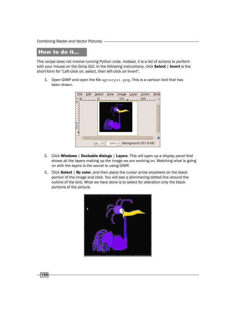
Combining Raster and Vector Pictures
150
How to do it...This recipe does not involve running Python code. Instead, it is a list of actions to perform with your mouse on the Gimp GUI. In the following instructions, click Select | Invert is the short-form for "Left-click on, select, then left-click on Invert".
1. Open GIMP and open the file apteryx1.png. This is a cartoon bird that has been drawn.
2. Click Windows | Dockable dialogs | Layers. This will open up a display panel that shows all the layers making up the image we are working on. Watching what is going on with the layers is the secret to using GIMP.
3. Click Select | By color, and then place the cursor arrow anywhere on the black portion of the image and click. You will see a shimmering dotted line around the outline of the bird. What we have done is to select for alteration only the black portions of the picture.

Chapter 7
151
4. Click Select | Invert. What this does is it changes the selection to everything except the black portion.
5. Click Edit | Copy. This picks up a copy of the selected portion (everything not black) and places it onto an invisible clipboard.
6. Click Edit | Paste. This takes a copy from the clipboard and potentially pastes it onto our existing image. But until you have completed the next step, the pasted image is held in a kind of no-man's land.
7. Click Layer | New. This firmly places the pasted portion of the image onto its own separate layer. The layers are like sheets of clear glass with portions of a composite picture on it. When you work on them and change one layer, the others are unaltered.
8. Right-click the Backdrop layer as shown, then click Delete Layer. This discards the Backdrop layer that consists of the original image. You will see there is only one layer left. It contains the bird image placed on a transparent background.

Combining Raster and Vector Pictures
152
9. Click File | Save as. In the save window, type in apteryx1.gif for the file name.
10. Close GIMP. You will find your new GIF image with a transparent background in whatever folder you sent it to. In Linux systems, transparent areas are shown as a gray checker-board pattern.
How it works...All images used in this chapter that have areas which are transparent were prepared using GIMP this way. There are other ways to achieve this but this is possibly the most readily available one. The animations in this chapter consist of a smaller, partially transparent image moving across a larger opaque image.
Diplomat walking at the palaceWe now animate a dignified man using the same legs as before, appropriately colored. For the human style walk, we need to select the correct mammalian knee-bend angle option chosen in the code prior to interpreting.

Chapter 7
153
Getting readyWe need the following GIF images:
A background picture of a suitable landscape
A human body without legs
A pair of sober shoes for dignity
The walking mammal legs
The images used are palace.gif, ambassador.gif, and ambassador_shoe1.gif. As before, the images of the man and the shoe have transparent backgrounds.
How to do it...Execute the program shown as before.
# walking_toff_1.py# >>>>>>>>>>>>>>>>>from Tkinter import *import mathimport timeroot = Tk()root.title("A Walking Toff in Natural Habitat - gif images")cw = 800 # canvas widthch = 200 # canvas height#GRAVITY = 4 chart_1 = Canvas(root, width=cw, height=ch, background="white")chart_1.grid(row=0, column=0)
cycle_period = 120 # time between new positions of the man # (milliseconds).im_backdrop = "/constr/pics1/toff_bg.gif"im_toff = "/constr/pics1/ambassador.gif"im_shoe = "/constr/pics1/toff_shoe.gif"toff =PhotoImage(file= im_toff)shoey =PhotoImage(file= im_shoe)backdrop = PhotoImage(file= im_backdrop)chart_1.create_image(0 ,0 ,anchor=NW, image=backdrop)base_x = 20base_y = 190hip_h = 60thy = 25#============================================

Combining Raster and Vector Pictures
154
# Hip positions: Nhip = 2 x Nstep, the number of steps per foot per # stride.hip_x = [0, 5, 10, 15, 20, 25, 30, 35, 40, 45, 50, 55, 60, 60, 60] #15hip_y = [0, 4, 6, 8, 6, 4, 0, 0, 0, 4, 6, 8, 6, 4, 0] #15
step_x = [0, 10, 20, 30, 40, 50, 60, 60] # 8 = Nhipstep_y = [0, 15, 25, 30, 25, 22, 10, 0]#============================================# Given a line joining two points xy0 and xy1, the base of an # isosceles triangle,# as well as the length of one side, "thy" this returns the # coordinates of# the apex joining the equal-length sides.
def kneePosition(x0, y0, x1, y1, thy): theta_1 = math.atan2((y1 - y0), (x1 - x0)) L1 = math.sqrt( (y1 - y0)**2 + (x1 - x0)**2) if L1/2 < thy: alpha = math.acos(L1/(2*thy)) else: alpha = 0.0 theta_2 = alpha + theta_1 x_knee = x0 + thy * math.cos(theta_2) y_knee = y0 + thy * math.sin(theta_2) return x_knee, y_knee
def animdelay(): chart_1.update() # Refresh the drawing on the canvas. chart_1.after(cycle_period) # Pause execution for 120 # milliseconds. chart_1.delete("walking") # Erases everything on the canvas.
bx_stay = base_xby_stay = base_y
for j in range(0,13): # Number of steps to be taken - # arbitrary. astep_x = 60*j bstep_x = astep_x + 30 cstep_x = 60*j + 15 aa = len(step_x) -1 for k in range(0,len(hip_x)-1): # Motion of the hips in a stride of each foot.

Chapter 7
155
cx0 = base_x + cstep_x + hip_x[k] cy0 = base_y - hip_h - hip_y[k] cx1 = base_x + cstep_x + hip_x[k+1] cy1 = base_y - hip_h - hip_y[k+1]
if k >= 0 and k <= len(step_x)-2: # Trajectory of the right foot. ax0 = base_x + astep_x + step_x[k] ax1 = base_x + astep_x + step_x[k+1] ay0 = base_y - 10 - step_y[k] ay1 = base_y - 10 -step_y[k+1] ax_stay = ax1 ay_stay = ay1
if k >= len(step_x)-1 and k <= 2*len(step_x)-2: # Trajectory of the left foot. bx0 = base_x + bstep_x + step_x[k-aa] bx1 = base_x + bstep_x + step_x[k-aa+1] by0 = base_y - 10 - step_y[k-aa] by1 = base_y - 10 - step_y[k-aa+1] bx_stay = bx1 by_stay = by1 # The shoes chart_1.create_image(ax_stay-5 ,ay_stay + 10 ,anchor=SW, \ image=shoey, tag="walking") chart_1.create_image(bx_stay-5 ,by_stay + 10 ,anchor=SW, \ image=shoey, tag="walking")
# Work out knee positions aknee_xy = kneePosition(ax_stay, ay_stay, cx1, cy1, thy) bknee_xy = kneePosition(bx_stay, by_stay, cx1, cy1, thy)
# Right calf. chart_1.create_line(ax_stay, ay_stay-5 ,aknee_xy[0], \ aknee_xy[1], width = 5, fill="black", tag="walking") # Right thigh. chart_1.create_line(cx1, cy1 ,aknee_xy[0], aknee_xy[1], \ width = 5, fill="black", tag="walking") # Left calf. #bknee_xy = kneePosition(bx_stay, by_stay, cx1, cy1, thy)

Combining Raster and Vector Pictures
156
chart_1.create_line(bx_stay, by_stay-5 ,bknee_xy[0], \ bknee_xy[1], width = 5, fill="black", tag="walking") # Left thigh. chart_1.create_line(cx1, cy1 ,bknee_xy[0], bknee_xy[1], \ width = 5, fill="black", tag="walking") # Torso chart_1.create_image(cx1-20 ,cy1+30 ,anchor=SW, \ image=toff, tag="walking")
animdelay() # Animation
root.mainloop()
How it works...The great possibilities offered through the use of image combining using the transparent channel in GIF images allows us to create studio-quality cartoon animations. The same remarks concerning the trigonometry made in the previous recipe apply here.
Spider in the forestWe now combine both mammal and bird leg motions to create a sinister-looking spider. We also introduce a moving background for the first time. No transparent images are used here as the entire spider is made of animated vector lines and ovals.
Getting readyHere, we need one long narrow strip image that is substantially wider than the Tkinter canvas provided. This not a problem and aids us in creating the illusion of a spider walking through an endless forest.
Dow
nlo
ad fro
m W
ow
! eBook
<w
ww
.wow
ebook.
com
>

Chapter 7
15�
How to do it...Execute the program shown as before.
# walker_spider_1.py# >>>>>>>>>>>>>>>>from Tkinter import *import mathimport timeroot = Tk()root.title("Mr Incy Wincy")cw = 500 # canvas widthch = 100 # canvas height chart_1 = Canvas(root, width=cw, height=ch, background="white")chart_1.grid(row=0, column=0)
cycle_period = 100 # time between new positions of thespider # (milliseconds).
base_x = 20base_y = 100avian = 1
ax = [ base_x, base_x+20, base_x+60 ]ay = [ base_y, base_y, base_y ]bx = [ base_x+90, base_x+130, base_x+170]by = [ base_y, base_y, base_y ]
cx1 = base_x + 80cy1 = base_y - 20thy = 50#=============================================posn_x = 0posn_y = 00
spider_backg = PhotoImage(file = "/constr/pics1/jungle_strip_1.gif")
#===========================================
foot_lift = [10,10,5,-5,-10,-10] # 3 legs per side, each foot in # sequence = 18 movesfoot_stay = [ 0, 0,0, 0, 0, 0]
Combining Raster and Vector Pictures
15�
#========================================# Given a line joining two points xy0 and xy1, the base of an # isosceles triangle,# as well as the length of one side, "thy" this returns the # coordinates of# the apex joining the equal-length sides - the position of the knee.
def kneePosition(x0, y0, x1, y1, thy, avian): theta_1 = math.atan2((y1 - y0), (x1 - x0)) L1 = math.sqrt( (y1 - y0)**2 + (x1 - x0)**2) if L1/2 < thy: # The sign of alpha determines which way the knees bend. if avian == 1: alpha = -math.acos(L1/(2*thy)) # Avian else: alpha = math.acos(L1/(2*thy)) # Mammalian else: alpha = 0.0 theta_2 = alpha + theta_1 x_knee = x0 + thy * math.cos(theta_2) y_knee = y0 + thy * math.sin(theta_2) return x_knee, y_knee
def animdelay(): chart_1.update() # This refreshes the drawing on the # canvas. chart_1.after(cycle_period) # This makes execution pause for 100 # milliseconds. chart_1.delete(ALL) # This erases *almost* everything on # the canvas.
for j in range(0,11): # Number of steps to be taken - arbitrary.
posn_x -= 1 chart_1.create_image(posn_x,posn_y,anchor=NW, image=spider_backg) for k in range(0,len(foot_lift)*3): posn_x -= 1 chart_1.create_image(posn_x,posn_y,anchor=NW, \ image=spider_backg) #cx1 += 3.5 cx1 += 2.6 # Phase 1 if k >= 0 and k <= 5: ay[0] = base_y - 10 - foot_lift[k] ax[0] += 8
Chapter 7
15�
by[0] = base_y - 10 - foot_lift[k] bx[0] += 8
# Phase 2 if k > 5 and k <= 11: ay[1] = base_y - 10 - foot_lift[k-6] ax[1] += 8 by[1] = base_y - 10 - foot_lift[k-6] bx[1] += 8
# Phase 3 if k > 11 and k <= 17: ay[2] = base_y - 10 - foot_lift[k-12] ax[2] += 8 by[2] = base_y - 10 - foot_lift[k-12] bx[2] += 8
for i in range(0,3): aknee_xy = kneePosition(ax[i], ay[i], cx1, cy1, thy, 1) # Mammal knee bknee_xy = kneePosition(bx[i], by[i], cx1, cy1, thy, 0) # Bird knee chart_1.create_line(ax[i], ay[i] ,aknee_xy[0], \ aknee_xy[1], width = 3) chart_1.create_line(cx1, cy1 ,aknee_xy[0], \ aknee_xy[1], width = 3) chart_1.create_line(bx[i], by[i] ,bknee_xy[0], \ bknee_xy[1], width = 3) chart_1.create_line(cx1, cy1 ,bknee_xy[0], \ bknee_xy[1], width = 3)
chart_1.create_oval(cx1-15 ,cy1-10 ,cx1+15 , \ cy1+10, fill="black") animdelay()
root.mainloop()
How it works...The essential art in making the spider walk acceptably is to adjust the length of stride, height of body above the ground, and thigh (leg segment) length to be consistent with each other. With slightly wrong adjustments, the legs roll over or appear made of very stretchy material.
There is also the issue of how the spider's leg movements should be synchronized. In this recipe, we have opted to make the limbs move in paired sequences.
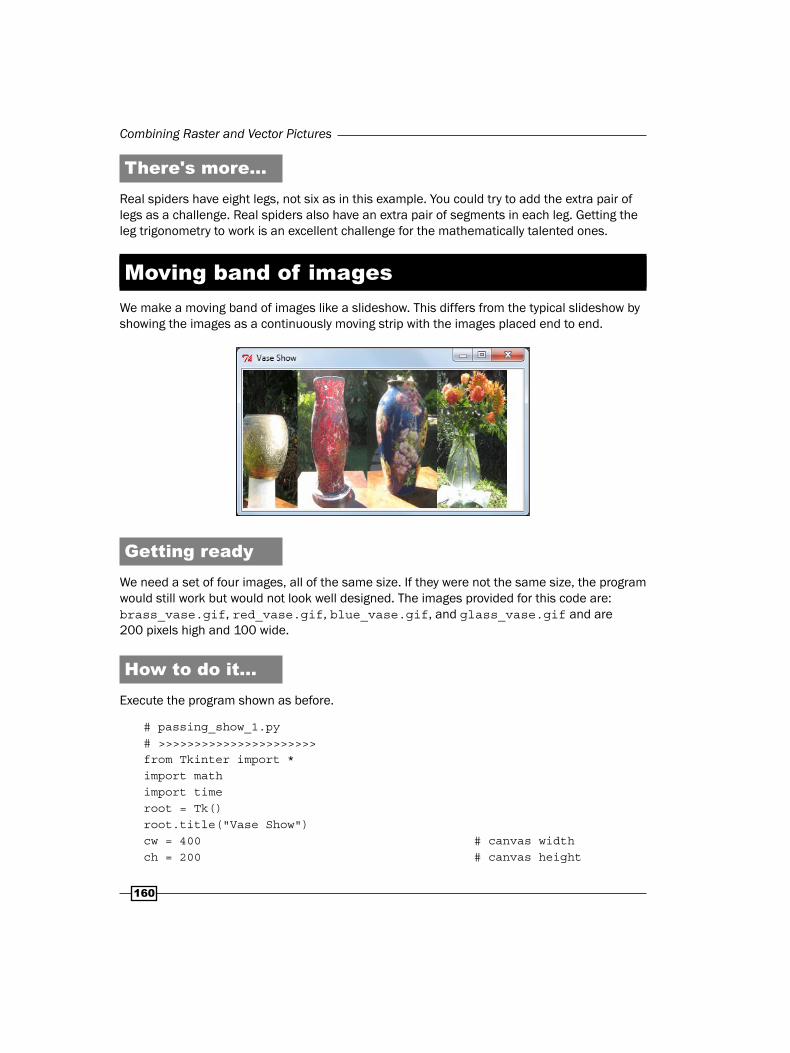
Combining Raster and Vector Pictures
160
There's more...Real spiders have eight legs, not six as in this example. You could try to add the extra pair of legs as a challenge. Real spiders also have an extra pair of segments in each leg. Getting the leg trigonometry to work is an excellent challenge for the mathematically talented ones.
Moving band of imagesWe make a moving band of images like a slideshow. This differs from the typical slideshow by showing the images as a continuously moving strip with the images placed end to end.
Getting readyWe need a set of four images, all of the same size. If they were not the same size, the program would still work but would not look well designed. The images provided for this code are: brass_vase.gif, red_vase.gif, blue_vase.gif, and glass_vase.gif and are 200 pixels high and 100 wide.
How to do it...Execute the program shown as before.
# passing_show_1.py# >>>>>>>>>>>>>>>>>>>>>>from Tkinter import *import mathimport timeroot = Tk()root.title("Vase Show")cw = 400 # canvas widthch = 200 # canvas height

Chapter 7
161
chart_1 = Canvas(root, width=cw, height=ch, background="white")chart_1.grid(row=0, column=0)
cycle_period = 100 # time between new positions of the ball (milliseconds).#=======================================================================posn_x1 = 0posn_x2 = 100posn_x3 = 200posn_x4 = 300
posn_y = 00
im_brass = PhotoImage(file = "/constr/pics1/brass_vase.gif")im_red = PhotoImage(file = "/constr/pics1/red_vase.gif")im_blue = PhotoImage(file = "/constr/pics1/blue_vase.gif")im_glass = PhotoImage(file = "/constr/pics1/glass_vase.gif")#=======================================================================def animdelay(): chart_1.update() # This refreshes the drawing on the canvas. chart_1.after(cycle_period) # This makes execution pause for 100 milliseconds. chart_1.delete(ALL) # This erases *almost* everything on the canvas.
for j in range(0,400): # Number of steps to be taken - arbitrary. posn_x1 -= 1 posn_x2 -= 1 posn_x3 -= 1 posn_x4 -= 1 chart_1.create_image(posn_x1,posn_y,anchor=NW, image=im_brass) chart_1.create_image(posn_x2,posn_y,anchor=NW, image=im_red) chart_1.create_image(posn_x3,posn_y,anchor=NW, image=im_blue) chart_1.create_image(posn_x4,posn_y,anchor=NW, image=im_glass) animdelay()
root.mainloop()# >>>>>>>>>>>>>>>>>>>>>>>>>>>>>>>>>>>>>>>>>>>>>>>>>>>>>>>
Combining Raster and Vector Pictures
162
How it works...Each image has its own x position coordinate posn_x1, posn_x2 etc. A 'for' loop adjusts these positions by one pixel each time the loop is executed, causing the images to progressively shift to the left.
Continuous band of imagesThis recipe extends the position-adjusting mechanism used in the previous example to sustain a continuous strip of images.
Getting readyWe use the same set of four images that were used in the previous recipe.
How to do it...Execute the program shown in exactly the same way as before.
# endless_passing_show_1.py# >>>>>>>>>>>>>>>>>>>>>from Tkinter import *import mathimport timeroot = Tk()root.title("Vase Show")cw = 100 # canvas widthch = 200 # canvas height chart_1 = Canvas(root, width=cw, height=ch, background="black")chart_1.grid(row=0, column=0)
cycle_period = 100 # time between new positions of the images milliseconds).#==============================================posn_x1 = 0posn_x2 = 100posn_x3 = 200posn_x4 = 300posn_y = 00
im_brass = PhotoImage(file = "/constr/pics1/brass_vase.gif")im_red = PhotoImage(file = "/constr/pics1/red_vase.gif")

Chapter 7
163
im_blue = PhotoImage(file = "/constr/pics1/blue_vase.gif")im_glass = PhotoImage(file = "/constr/pics1/glass_vase.gif")#=============================================def animdelay(): chart_1.update() # This refreshes the drawing on the canvas. chart_1.after(cycle_period) # This makes execution pause for 100 milliseconds. chart_1.delete(ALL) # This erases *almost* everything on the canvas.
for j in range(0,600): # Number of steps to be taken - arbitrary. posn_x1 -= 1 posn_x2 -= 1 posn_x3 -= 1 posn_x4 -= 1 chart_1.create_image(posn_x1,posn_y,anchor=NW, image=im_brass) chart_1.create_image(posn_x2,posn_y,anchor=NW, image=im_red) chart_1.create_image(posn_x3,posn_y,anchor=NW, image=im_blue) chart_1.create_image(posn_x4,posn_y,anchor=NW, image=im_glass) # The numerical parameters below could be turned into # a 'for' loop and allow the loop to be compact and interminable. if j == 100: posn_x1 = 300 if j == 200: posn_x2 = 300 if j == 400: posn_x3 = 300 if j == 400: posn_x4 = 300 animdelay()
root.mainloop()
How it works...The trick with this program is to reset the x position coordinates, posn_1, and so on, which control the position of each image on the canvas after the image has exited the canvas on the left. The position coordinates get reset to a position 200 pixels off to the right of the canvas.

Combining Raster and Vector Pictures
164
Endless backgroundThe next thing to achieve is to create what appears to be one practically infinitely wide panorama. We extend the technique used in the previous example and make a background image that appears to be endless.
Getting readyWe have provided a single image that has been doctored so that the right-hand edge fits exactly onto the left-hand edge to create an endless and continuous image if they are placed side by side. The GIMP image manipulation program was used to do this editing. In a very condensed explanation, we do the following:
1. We copy a portion of the image that does not have too much detail vertically where we make the cut.
2. This is then pasted onto one end so that there is substantial overlap of the two images.
3. Then the top layer, containing the copy-and-pasted portion, has the eraser tool with a fuzzy edge applied so that we cannot see the transition from one image to the next.
How to do it...Execute the following code.
# passing_cloudscape_1.py# >>>>>>>>>>>>>>>>from Tkinter import *import timeroot = Tk()

Chapter 7
165
root.title("Freedom Flight Cloudscape")cw = 400 # canvas widthch = 239 # canvas height chart_1 = Canvas(root, width=cw, height=ch, background="black")chart_1.grid(row=0, column=0)
cycle_period = 50 # time between new positions of the background # (milliseconds).#=============================================posn_x1 = 0posn_x2 = 574posn_plane_x = 60posn_plane_y = 60posn_y = 00# Panorama image size = 574 x 239im_one = PhotoImage(file = "/constr/pics1/continuous_clouds \ _panorama.gif")im_two = PhotoImage(file = "/constr/pics1/continuous_clouds \ _panorama.gif")im_plane = PhotoImage(file = "/constr/pics1/yellow_airplane_2.gif")#===========================================def animdelay(): chart_1.update() # This refreshes the drawing on the # canvas. chart_1.after(cycle_period) # This makes execution pause for 50 # milliseconds. chart_1.delete(ALL) # This erases *almost* everything on # the canvas.num_cycles = 10 # Number of total cycles of the # loop.k = 0for j in range(0,num_cycles*1148): # Number of steps to be taken # arbitrary. posn_x1 -= 1 posn_x2 -= 1 k += 1 chart_1.create_image(posn_x1,posn_y,anchor=NW, image=im_one) chart_1.create_image(posn_x2,posn_y,anchor=NW, image=im_two) chart_1.create_image(posn_plane_x,posn_plane_y,anchor=NW, \ image=im_plane) if k == 574: posn_x1 = 574 if k == 1148: posn_x2 = 574

Combining Raster and Vector Pictures
166
k = 0 posn_x1 = 0 animdelay()
root.mainloop()
How it works...We use the same x coordinate position adjustment technique as we did in the previous recipe. This time we choose the position for readjustment to be a multiple of 574 which is the width, in pixels, of the cloudscape image. We also use the image of an airplane, on a transparent background. The airplane is kept stationary.

�Data In and Data Out
In this chapter, we will cover:
Creating a new file on the hard drive
Writing data to a newly created file
Writing data to multiple files
Adding data to existing files
Saving a Tkinter drawing shape to disk
Retrieving Python data from disk
Simple mouse input
Storing and retrieving a mouse-drawn shape
A mouse-line editor
All possible mouse actions
IntroductionNow we address the technicalities of storing and retrieving graphic data on storage media like hard disks. Besides raster images, we need to be able to create, store, and retrieve vector graphics of ever increasing complexity. We also want techniques for transforming portions of raster images into vector images.
Till now, all our programs have carried their data inside the source code. This limits the complexity of the data lists and arrays that we can conveniently type in a few minutes. We do not want this limitation. We want to be able to handle and manipulate blocks of raw data that may be hundreds of megabytes in size if necessary. Typing in such files by hand is unthinkably inefficient. There are better ways of doing things. This is what named-files, data streams, and hard drives are for.

Data In and Data Out
16�
Creation of a new file on a hard driveWe write and execute the simplest program that will create a data file on disk.
Till now, it was not required to store any data on our hard drive or a USB memory stick. Now we work through a series of simple exercises in storing and retrieving data in files on storage media. Then we use these methods to save and edit Tkinter lines in a practical way. Tkinter lines can be a large collection of separate line segments and shapes. If we are developing a drawing of complexity and richness, it is vital that we be able to store and retrieve work in progress.
How to do it...Write, save, and execute the program shown in the usual way. When you run the program, all you will observe from a successful execution is a short pause after you have clicked Enter. The execution will terminate without any messages. However, a new file called brand_new_file.dat now exists on the destination directory constr. We should open constr and verify that this is indeed the case.
# file_make_1 .py# >>>>>>>>>>>>>>filename = "constr/brand_new_file.dat"FILE = open(filename,"w")
How it works...This minimalist-looking program achieves the following objectives:
It verifies that Python's file IO functions are present and working. No modules need to be imported
It demonstrates that there is nothing unusual about the way Python accesses data files on storage devices
It proves that the operating system obeys file creation directives from Python
How to read the newly created fileOnce a file has been created, it can then be read. So a program to read an existing file on disk would be:
# file_read_1 .py# >>>>>>>>>>>filename = "constr/brand_new_file.dat"FILE = open(filename,"r")
Dow
nlo
ad fro
m W
ow
! eBook
<w
ww
.wow
ebook.
com
>

Chapter 8
16�
As you can see, the only difference is the r instead of the w.
Note that Python reads and writes files in more than one format. A b as in rb and wb reads and writes as byte or binary format. These are the 1s and 0s in each byte. r and w without the b as in our examples tells the Python interpreter that it must interpret the bytes as ASCII characters. The only point we need to remember is to keep the formats separate.
Writing data to a newly-created fileWe now create a file and then write a small amount of data to it. The value of these very, very simple recipes is that when we are trying some task that is complex and things do not work as expected, the simple one-action-only test programs allow us to break our problem down into simple tasks that we can gradually add complexity to, verifying the validity of each new change. This is a tried and trusted philosophy used by many of the best programmers.
# file_write_1.py#>>>>>>>>>>>>># Let's create a file and write it to disk.filename = "/constr/test_write_1.dat"filly = open(filename,"w") # Create a file object, in write # mode
for i in range(0,2): filly.write("everything inside quotes is a string, even 3.1457") filly.writelines("\n") filly.write("How will stored data be delimited so we can read \ chunks of it into elements of list, tuple or dictionart?") filly.writelines("\n")#filly.close()
How it works...The important thing to note at this point is that the newline character \n is the natural way by which Python separates variables. Space characters will also be used as number or character value separators or delimiters.
Writing data to multiple filesWe see here that opening and writing data to a series of separate files is, as we have come to expect from Python, very simple and straightforward. Once we have seen an example of the correct syntax, it just works.
# file_write_2.py#>>>>>>>>>>>>># Let's create a file and write it to disk.

Data In and Data Out
1�0
filename_1 = "/constr/test_write_1.dat"filly = open(filename_1,"w") # Create a file object, in # write modefilly.write("This is number one and the fun has just begun")
filename_2 = "/constr/test_write_2.dat"filly = open(filename_2,"w") # Create a file object, in # write modefilly.write("This is number two and he has lost his shoe")
filename_3 = "/constr/test_write_3.dat"filly = open(filename_3,"w") # Create a file object, in # write modefilly.write("This is number three and a bump is on his knee")#filly.close()
How it works...The value of this example is that it provides examples of correct debugged syntax. So it is available for reuse and modification with the minimum of bother.
Adding data to existing filesWe test three ways of writing data to existing files in order to discover some basic rules of data storage.
# file_append_1.py#>>>>>>>>>>>>>>>>># Open an existing file and add (append) data to it.filename_1 = "/constr/test_write_1.dat"filly = open(filename_1,"a") # Open a file in append modefilly.write("\n")filly.write("This is number four and he has reached the door")
for i in range(0,5): filename_2 = "/constr/test_write_2.dat" filly = open(filename_2,"a") # Create a file in append mode filly.write("This is number five and the cat is still alive")
filename_3 = "/constr/test_write_2.dat"filly = open(filename_3,"w") # Open an existing file in # write mode
# The command below WILL fail – "w" is really "overwrite"filly.write("This is number six and they cannot find the fix")
Chapter 8
1�1
How it works...What make up the first method are two things: firstly, we open the file for appending ("a") which means we will add data to what is already in the file. Nothing will be destroyed or overwritten. Secondly, we separate the new data from the old with the line
filly.write("\n")
The second method works, but is a very bad practice because there is no way of separating different entries.
The third method wipes out whatever was previously stored in the file.
So remember the difference between write and appendIf we keep the above three methods clear in our heads, we will be able to successfully store and retrieve our data without mishap and frustration.
Saving a Tkinter-drawing shape to diskWhen we create an elaborate shape using Tkinter, we often want to preserve that shape for later use. In fact, we would like to build up a whole library of shapes. If other people do similar work, we may want to share and exchange shapes. Such community efforts are the key to the success of the most powerful and successful open-source programs.
Getting readyIf we go back to the example titled "Drawing Intricate Shapes – the Curly Vine", in Chapter 2, Drawing Fundamental Shapes, we see that the shapes are defined by the two coordinate lists vine_x and vine_y. We are going to first save these shapes in a disk file and then see what is needed to successfully retrieve and draw them.
Create a folder /constr/vector_shapes on your hard drive ready to receive your stored data.
How to do it...Execute the program shown in the usual way.
# save_curly_vine_1.py#>>>>>>>>>>>>>>>>>vine_x = [23, 20, 11, 9, 29, 52, 56, 39, 24, 32, 53, 69, 63, \ 47, 35, 35, 51,\ 82, 116, 130, 95, 67, 95, 114, 95, 78, 95, 103, 95, 85, 95, 94.5]
Data In and Data Out
1�2
vine_y = [36, 44, 39, 22, 16, 32, 56, 72, 91, 117,125, 138, 150, \ 151, 140, 123, 107,\ 92, 70, 41, 5, 41, 66, 41, 24, 41, 53, 41, 33, 41, 41, 39]
vine_1 = open('/constr/vector_shapes/curley_vine_1.txt', 'w')
vine_1.write(str(vine_x ))vine_1.write("\n")vine_1.write(str(vine_y ))
How it works...The first thing to note is that stored data does not have a 'type' – it is just text characters. So any data being appended to an open file must be converted into string format using the string conversion function str(some_integer_or_float_object).
The second thing to note is that storing the whole list as a list object, like str(vine_x), is the best way to do things because when stored this way it can be read back directly as a whole line read into a similar list object– see the next recipe to how to do this. In typical Python fashion, the simple and obvious method always seems to be the best.
Storing commandsThe problem we face when retrieving lists of mixed integer and floating point data is that it is stored as a long string of characters. So how do we get Python to convert the long lists of characters that include square brackets, commas, spaces and new-line characters, into a normal Python numerical list? We want our drawing back undamaged. There is a lovely function eval() that does this effortlessly.
There is another method called pickle that does the same thing.
Retrieving Python data from disk storageWe retrieve two lists vine_x and vine_y from the stored file curley_vine_1.txt. We want them to be in exactly the same form they were in before they were sent for storage.
Getting readyThe preparation for this recipe was done by running the previous program save_curly_vine_1.py. If this ran successfully, there will be a file curly_vine_1.txt inside /constr/vector_shapes. If you open the text file you will see two lines, the first line being the string representation of our original vine_x and similarly the second line of this file will represent vine_y.
Chapter 8
1�3
# retrieve_curly_vine_1.py#>>>>>>>>>>>>>>>>>>>>>#vine_x = []vine_1 = open('/constr/vector_shapes/curley_vine_1.txt', 'r')
vine_x = eval(vine_1.readline())vine_y = eval(vine_1.readline())
# Tests to confirm that everything worked.print "vine_x = ",vine_xprint vine_x[31]print "vine_y = ",vine_yprint vine_y[6]
How it works...This works so simply and elegantly because of the eval() function. The documentation says: "The expression argument is parsed and evaluated as a Python expression" and "The return value is the result of the evaluated expression". This is a way of saying that the text inside the brackets is treated as if it were plain Python expressions and executed as such. In our particular example, the string inside the curly brackets is interpreted as a list of numbers, not characters which is what we desire.
Simple mouse inputWe now develop code that helps to draw complicated shapes by capturing mouse clicks on electronic graph paper rather than with a pencil, eraser, and sheets of paper made from dead trees. We break this complex task into simple steps covered by the next three recipes.
# mouseclick_1.py#>>>>>>>>>>>>>>>from Tkinter import *root = Tk()
frame = Frame(root, width=100, height=100)
def callback(event): print "clicked at", event.x, event.y
frame.bind("<Button-1>", callback)frame.grid()
root.mainloop()root.destroy()

Data In and Data Out
1�4
How it works...Clicking a mouse button is referred to as an event. If we want our program to perform some actions within our program, then we need to write a callback function that is called whenever the event occurs. Older terminology for callback was "interrupt service routine".
The line frame.bind("<Button-1>", callback) says in effect:
"Make a connection (bind()) between the event, which is the click of the left button on the mouse (<Button-1>), and the function called callback". You could name this function anything you like, but the word callback makes the code easier to understand.
The final point to note is that the variables event.x and event.y are reserved for recording the x-y coordinates of the mouse. In this specific callback function we print out the position, in a frame called "frame", of the mouse when clicked.
There's more...We build on the use of mouse-triggered callback functions in the next two recipes with the objective of producing a shape-tracing tool.
Storing and retrieving a mouse-drawn shapeWe make a program that lets you create a shape through the use of the mouse and by means of three buttons we can store the shape on disk, clear the canvas and then recall and display the shape on the screen.
Getting readyEnsure you have created a folder call constr because this is where the code in our program expects to be able to save the shape drawn. It is also where it will retrieve it from when commanded to retrieve and display it.
# mouse_shape_recorder_1.py#>>>>>>>>>>>>>>>>>>>>>from Tkinter import *root = Tk()root.title("Mouse Drawn Shape Saver")cw = 600 # canvas widthch = 400 # canvas heightchart_1 = Canvas(root, width=cw, height=ch, background="#ffffff")chart_1.grid(row=1, column=1)

Chapter 8
1�5
pt = [0]x0 = [0]y0 = [0]count_point = 0x_end = 10y_end = 10#============================================# Create a new circle where the click happens and draw a new line# segment to the last point (where the mouse was left clicked).def callback_1(event): # Left button pressed. global count_point, x_end, y_end global x0, y0 global x0_n, y0_n, pt
x_start = x_end y_start = y_end x_end = event.x y_end = event.y chart_1.create_line(x_start, y_start , x_end,y_end , fill = \ "#0088ff") chart_1.create_oval(x_end-5,y_end-5, x_end+5, y_end+5, outline = \ "#0088ff")
count_point += 1 pt = pt + [count_point] x0 = x0 + [x_end] # extend list of all points y0 = y0 + [y_end]
chart_1.bind("<Button-1>", callback_1) # <button-1> left mouse button#==============================================# 1. Button control to store segmented linedef callback_6(): global x0, y0 xy_points = open('/constr/shape_xy_1.txt', 'w') xy_points.write(str(x0)) xy_points.write('\n') xy_points.write(str(y0)) xy_points.close()
Button(root, text="Store", command=callback_6).grid(row=0, column=2)#=============================================# 2. Button control to retrieve line from file.def callback_7():

Data In and Data Out
1�6
global x0, y0 # Stored list of mouse-click positions. xy_points = open('/constr/shape_xy_1.txt', 'r') x0 = eval(xy_points.readline()) y0 = eval(xy_points.readline()) xy_points.close() print "x0 = ",x0 print "y0 = ",y0
for i in range(1, count_point): # Re-plot the stored and # retreived line chart_1.create_line(x0[i], y0[i] , x0[i+1], y0[i+1] , \ fill = "#0088ff") chart_1.create_oval(x_end - 5,y_end - 5, x_end + 5, \ y_end + 5 , outline = "#0088ff")
Button(root, text="retrieve", command=callback_7).grid(row=1, \ column=2)#=============================================# 3. Button control to clear canvasdef callback_8(): chart_1.delete(ALL)
Button(root, text="CLEAR", command=callback_8).grid(row=2, column=2)
root.mainloop()
How it works...In addition to a callback function for adding the positions of left mouse clicks to lists x0 and y0, of x and y-coordinates, we have another three callback functions. The three additional callback functions are to trigger the execution of functions that:
Save the lists x0 and y0 to a disk in a file called shape_xy_1.txt.
Clear the canvas of all drawn lines and circles
Retrieve the contents of shape_xy_1.txt and re-draw it onto the canvas
There's more...Drawing is an imperfect process and artists and draughtsman use an eraser as well as a pencil. When we make drawings with a mouse connected to a computer we also need to make adjustments and corrections to any lines we draw. We need editing ability.

Chapter 8
1��
We need to edit mistakesDrawing is an imperfect process. We would like to be able to adjust the position of some of the points in order to improve the drawing. We do this in the next recipe.
A mouse-line editorWe edit (change) a shape drawn using the mouse after the drawing is finished.
Getting readyTo limit the complexity and length of the code, we have excluded the facilities provided in the previous recipe for storing and recalling the drawn shape. So for this recipe no storage folders will be used.
# mouse_shape_editor_1.py#>>>>>>>>>>>>>>>>>>>>>>>>>>>>>>>>>>>>>>>>>>from Tkinter import *import mathroot = Tk()root.title("Left drag to draw, right to re-position.")cw = 600 # canvas widthch = 650 # canvas heightchart_1 = Canvas(root, width=cw, height=ch, background="#ffffff")chart_1.grid(row=1, column=1)
linedrag = {'x_start':0, 'y_start':0, 'x_end':0, 'y_end':0}map_distance = 0dist_meter = 0x_initial = 0y_initial = 0#==============================================# Adjust the distance between points if desiredway_points = 50 # Distance between editable way-points#==============================================magic_circle_flag = 0 # 0-> normal dragging, 1 -> double-click: # Pull point.point_num = 0x0 = []y0 = []#================================================

Data In and Data Out
1��
def separation(x_now, y_now, x_dot, y_dot): # DISTANCE MEASUREMENT # Distance to points - used to find out if the mouse # clicked inside a circle sum_squares = (x_now - x_dot)**2 + (y_now -y_dot)**2 distance= int(math.sqrt(sum_squares)) # Get Pythagorean # distance return( distance)#================================================# CALLBACK EVENT PROCESSING FUNCTIONSdef callback_1(event): # LEFT DOWN global x_initial, y_initial x_initial = event.x y_initial = event.y
def callback_2(event): # LEFT DRAG global x_initial, y_initial global map_distance, dist_meter global x0, y0 linedrag['x_start'] = linedrag['x_end'] # update positions linedrag['y_start'] = linedrag['y_end'] linedrag['x_end'] = event.x linedrag['y_end'] = event.y
increment = separation(linedrag['x_start'],linedrag['y_start'], \ linedrag['x_end'], linedrag['y_end'] ) map_distance += increment # Total distance - # potentiasl use as a map odometer. dist_meter += increment # Distance from last circle
if dist_meter>way_points: # Action at way-points x0.append(linedrag['x_end']) # append to line y0.append(linedrag['y_end']) xb = linedrag['x_end'] - 5 ; yb = linedrag['y_end'] - 5 # Centre circle on line x1 = linedrag['x_end'] + 5 ; y1 = linedrag['y_end'] + 5 chart_1.create_oval(xb,yb, x1,y1, outline = "green") dist_meter = 0 # re-zero the odometer. linexy = [ x_initial, y_initial, linedrag['x_end'] , \ linedrag['y_end'] ] chart_1.create_line(linexy, fill='green') x_initial = linedrag['x_end'] # start of next segment

Chapter 8
1��
y_initial = linedrag['y_end']
def callback_5(event): # RIGHT CLICK global point_num, magic_circle_flag, x0, y0 # Measure distances to each point in turn, determine if any are # inside magic circle. # That is, identify which point has been clicked on. for i in range(0, len(x0)): d = separation(event.x, event.y, x0[i], y0[i]) if d <= 5: point_num = i # this is the index that controls editing magic_circle_flag = 1 chart_1.create_oval(x0[i] - 10,y0[i] - 10, x0[i] + 10, \ y0[i] + 10 , width = 4, outline = "#ff8800") x0[i] = event.x y0[i] = event.y
def callback_6(event): # RIGHT RELEASE global point_num, magic_circle_flag, x0, y0 if magic_circle_flag == 1: # The point is going to be # repositioned. x0[point_num] =event.x y0[point_num] =event.y chart_1.delete(ALL) chart_1.update() # Refreshes the drawing on the # canvas. q=[] for i in range(0,len(x0)): q.append(x0[i]) q.append(y0[i]) chart_1.create_oval(x0[i] - 5,y0[i] - 5, x0[i] + 5, \ y0[i] + 5 , outline = "#00ff00") chart_1.create_line(q , fill = "#ff00ff") # Now show the # new positions magic_circle_flag = 0#==============================chart_1.bind("<Button-1>", callback_1) # <Button-1> ->LEFT mouse # buttonchart_1.bind("<B1-Motion>", callback_2)chart_1.bind("<Button-3>", callback_5) # <Button-3> ->RIGHT mouse # buttonchart_1.bind("<ButtonRelease-3>", callback_6)
root.mainloop()
Dow
nlo
ad fro
m W
ow
! eBook
<w
ww
.wow
ebook.
com
>
Data In and Data Out
1�0
How it works...The preceding program now includes:
callback functions to deal with left and right mouse clicks and drags.
A distance-measuring function separation(x_now, y_now, x_dot, y_dot). When the right mouse button is clicked, the distance to every line joint is measured. If one of these distances is inside an existing joint then an orange circle is drawn and control is passed to callback_6 which updates the coordinates of the new point and refreshes the revised drawing. The decision on whether to move a point or not is decided by the value of the magic_circle_flag. The state of this flag is determined by the distance computed by separation(). It is set to 1 if the distance measurement finds it inside a joint when the right mouse is pressed and set to 0 after a point has been moved.
There's more...Now that we have a means to control and adjust the drawing of lines and curves using mouse manipulation, other possibilities are opened up.
Why don't we add more features?It would be good to extend the features of this program to include:
The ability to erase points
The ability to work with unjoined segments
The ability to select or click to create points
Drag fairy lights (equal length segments)
The list will grow longer as we work on the extensions. In the end, we will have created a useful vector graphics editor and the pressure would be on to match features of existing proprietary and open-source editors. Why re-invent the wheel? What may bear more fruit would be an effort to work with vector images produced by an existing mature vector editor, if this is a practical option.
Using other tools to acquire and re-work imagesIn the next chapter, we explore ways and means of using vector images from the open-source vector graphics editor Inkscape. Inkscape is able to export images in a wide choice of formats including a standardized web format called Scaled Vector Graphics or SVG for short.

Chapter 8
1�1
How to exploit that mouseThis chapter has made much use of the mouse as a user-interaction tool for drawing shapes on Tkinter canvasses. To complete the job of acquiring the know-how of using the mouse to its fullest the next recipe will be an examination of the full toolkit of mouse interactions.
We can measure the distance along a meandering lineIn the code, there is a variable called map_distance that has not been used. It can be used to trace the distance travelled on meandering paths on maps. The idea is that if we wanted to measure distances on unmarked paths and roads on something like a Google map, we would be able to adapt this recipe to the task.
All possible mouse actionsNow we make a program that tests each possible mouse event that Python is capable of responding to.
How to do it...Execute the program shown in the normal way.
# all_mouse_actions_1.py#>>>>>>>>>>>>>>>>>>from Tkinter import *root = Tk()root.title("Mouse follower")# The Canvas here is bound to the mouse eventscw = 200 # canvas widthch = 100 # canvas heightchart_1 = Canvas(root, width=cw, height=ch, background="#ffffff")chart_1.grid(row=1, column=1)
#========= Left Mouse Button Events ===============# callback eventsdef callback_1(event): print "left mouse clicked"
def callback_2(event): print "left dragged"
def callback_3(event): print "left doubleclick"

Data In and Data Out
1�2
def callback_4(event): print "left released"#======== Center Mouse Button Events ======================def callback_5(event): print "center mouse clicked"
def callback_6(event): print "center dragged"
def callback_7(event): print "center doubleclick"
def callback_8(event): print "center released"#======== Right Mouse Button Events ======================def callback_9(event): print "right mouse clicked"
def callback_10(event): print "right dragged"
def callback_11(event): print "right doubleclick" def callback_12(event): print "right released"
# <button-1> is the left mouse buttonchart_1.bind("<Button-1>", callback_1)chart_1.bind("<B1-Motion>", callback_2)chart_1.bind("<Double-1>", callback_3)chart_1.bind("<ButtonRelease-1>", callback_4)
# <button-2> is the center mouse buttonchart_1.bind("<Button-2>", callback_5)chart_1.bind("<B2-Motion>", callback_6)chart_1.bind("<Double-2>", callback_7)chart_1.bind("<ButtonRelease-2>", callback_8)
# <button-3> is the right mouse buttonchart_1.bind("<Button-3>", callback_9)chart_1.bind("<B3-Motion>", callback_10)chart_1.bind("<Double-3>", callback_11)chart_1.bind("<ButtonRelease-3>", callback_12)
root.mainloop()#>>>>>>>>>>>>>>>>>>>>>>>>>>>>>>>>>>>>>>>>>>>>>>>>>>>>

Chapter 8
1�3
How it works...The preceding code is reasonably self-explanatory. A small canvas is created that is responsive to all the mouse actions. Proof that the responses are working correctly are by means of confirmation messages typed on the system console. We can adapt the callback functions to do any kind of task we choose simply by inserting appropriate Python commands into the callback functions.
There's more...Mouse events and Tkinter widgets often work together. Most Tkinter GUI widgets are designed to be controlled by mouse events such as left or right-clicks or dragging with a button held down. Tkinter provides a versatile selection of widgets and these will be explored in Chapter 10, GUI Construction Part 1 and Chapter 11, GUI Construction Part 2.

�Exchanging Inkscape
SVG Drawings with Tkinter Shapes
In this chapter, we will cover:
Inkscape as a tool for acquiring Tkinter line shapes (paths)
Finding and installing Inkscape
Where to find SVG clipart
Getting Tkinter paths from raster images
Converting path data from SVG images into other formats
Using Inkscape as a graphic tool for Tkinter paths
IntroductionIn this chapter, we explore alternate ways and means of getting graphic-shaped data into Tkinter programs. Probably the most widespread vector-graphic format is the one designed to work on web pages. This is known as SVG, which is short-form for Scaled Vector Graphics. It is the official standard specification defined by the World Wide Web Consortium and has been around since 1999.
Our interest in SVG comes from the practical use it has for us in creating drawn shapes in Python with the Tkinter module.

Exchanging Inkscape SVG Drawings with Tkinter Shapes
1�6
Professional vector-drawing packages like Inkscape and some of the proprietary-drawing packages allow us, aided by some Python code, to acquire lists of coordinates that can be used directly in the create_line(x0,y0 …) functions of Tkinter.
There are growing libraries of copyright-free SVG pictures available on the web. With tools like Inkscape, we can dismantle existing images and use parts of them for our own graphic work and Python programs. One such site is www.openclipart.org/ which allows and encourages anyone to copy the thousands of images stored there in SVG format.
SVG drawings encode lines in more than one way. One way is to represent a line as a series of x-y coordinate points on a canvas. Each point is defined as a pair of numbers referred to the zero position of the canvas which is the North-West corner (top-right). The second way is to represent each point as a relative shift from the previous point.
The structure of an SVG drawingWe shall examine how Inkscape encodes drawings so that we may interpret them for use in Python. What we will do is:
1. Draw some simple objects in Inkscape and save them somewhere as "Plain SVG" format files.
2. Then we open the files in a text editor and inspect the contents so that we can recognize the lines we are interested in.
3. Finally we write code that will convert the SVG lines of interest into Tkinter lists which we can use directly in our Python programs.
Getting readyThe first thing we need to do now is acquire and install a copy of Inkscape onto our computer. We will find this at www.inkscape.org/download/ where there are versions for Linux and Microsoft Windows.
The on-line documentation and tutorials for Inkscape are excellent. However, we want to use the minimum amount of Inkscape so this recipe is just that – a few pointers to get the minimum task done.
How to do it...The only tool we need to use in Inkscape is the line-drawing pen as shown in the following screenshot. We drew a "Z" shape with this tool and saved the file as z_inkscape.svg.

Chapter 9
1��
The code produced, displayed in a text editor is shown after the screenshot:
<?xml version="1.0" encoding="UTF-8" standalone="no"?><!-- Created with Inkscape (http://www.inkscape.org/) --><svgxmlns:svg="http://www.w3.org/2000/svg"xmlns="http://www.w3.org/2000/svg"version="1.1"width="744.09448"height="1052.3622"id="svg3741"><defsid="defs3743" /><gid="layer1"><path d="m 122.85714,89.50504 280,0 -280,45.71429 271.42857,0 "id="path3751" style="fill:none;stroke:#000000;stroke-width:1px;stroke-linecap:butt;stroke-linejoin:miter;stroke-opacity:1" /></g></svg>
How it works...Most of the preceding code is of no interest to us. It is the XML code that a web browser interprets in order to display a web page. Embedded within it, however, are SVG paths which we somehow want to transfer to Python so Tkinter can display it as a drawn shape.
Exchanging Inkscape SVG Drawings with Tkinter Shapes
1��
The portion we are interested in is the paragraph starting with <path as this is the SVG format description of the "Z" shape that was drawn with the pen tool. This is the section of code:
<path d="m 122.85714,89.50504 280,0 -280,45.71429 271.42857,0 " id="path3751" style="fill:none;stroke:#000000;stroke-width:1px;stroke- linecap:butt;stroke-linejoin:miter;stroke-opacity:1" />
This is the whole SVG description of the 'Zorro' sign and the following line, has been slightly simplified, by removing the decimal fractions, to improve readability:
d="m 122, 89 280,0 -280,45 271,0"
This line is the equivalent of a group of Tkinter instructions that could be written:
x0 = 122y0 = 89canvas.create_line(x0,y0, x0+280,y0+0, x0-280,y0+45, x0+271,y0,+0 )
The 'm' symbol is the SVG instruction "move-to" where the number of pixels moved are increments added to the coordinates of the previous point in the line – except for the first point 122,89 which tells the pen where to begin.
There's more...We do not want to become SVG experts. We only want to know enough to be able to recognize graphic data which we can use in Python. In this spirit, a summary of a few of the most common SVG directives is given here.
m x,y is the "move-to" instruction which moves the pen to the point x,y without drawing a line.
m x0,y0 x1,y1 x2,y2 will draw a line from x0,y0 to x1,y1 and then another segment from x1,y1 to x2, y2. Note that the SVG interpreter only interprets the first point x0,y0 as a "move-to" but interprets subsequent pairs of points as "line-to". "line-to" is an instruction to put the tip of the pen onto the surface and draw.
m x0,y0 x1,y1 x2,y2 will draw a line from x0,y0 to x0+x1,y0+y1 and then another segment from x0+x1,y0+y1 to x0+x2,y0+y2.
The point to note is that the use of lower case is significant and is telling the SVG interpreter to calculate the coordinates as increment values that must be added to the previous location. As with the m directive the pen moves to the first point x0,y0 without drawing anything, but all subsequent points are drawn as segments joining adjacent points.

Chapter 9
1��
l x,y commands the pen to draw a line from wherever the pen happens to be now to the point x,y.
l x,y commands the pen to draw a line from the current pen position (x0,y0 for instance) to the point x0 + x, y0 + y.
z at the end of a list of path coordinates will close the path by drawing a line from the current point back to the start point.
SVG code for separate pathsSeparate paths each get their own <path innards-of the path /> code.
Thus the SVG code for three separate paths could be as follows:
<path d="M 125,100 340,149 340,100"id="path3000"style="style-descriptors" /><path d="m 128,258 0,137 148,0 0,-145 -148,8 z"id="path3001"style="style-descriptors" /><path d="m 114,629 0,-134 0,122 102,0 0,-134 105,0 0,120 82,0 0,-114"id="path3002"style="style-descriptors " />
Our interest is in the three lines starting from d= because these give the strings of x,y pairs that give the location of points on a drawn shape. The high degree of arithmetic precision is redundant because Tkinter will only use the integer part. However, if we needed to scale the picture up by multiplying each number by an amplification factor then the high arithmetic precision would avoid a small amount of distortion of the shape.
Tracing the shape of an image in InkscapeWe want to use Inkscape to capture a complex series of shapes – ones that would be tedious and difficult to draw with pencil and paper. A practical example of the use of this could be that you may want to paint a picture of an elephant and you need some reliable guidelines, based on a magazine picture or photograph, for the outlines of the limbs and body. One way is to draw a grid on the picture with a pencil and ruler, then repeat a scaled version of the grid on blank canvas and finally to draw the outlines with a lead pencil. An alternative method is to pull a JPG, GIF, PNG, BMP, or TIFF image of the elephant into Inkscape and trace a series of lines over it using the pen tool. These outlines can be printed and traced onto your canvas. These same shapes can be used in Python with Tkinter.

Exchanging Inkscape SVG Drawings with Tkinter Shapes
1�0
There are other ways of converting raster images to SVG paths but they require a fair amount of pre-conditioning of the images such as color separation and converting continuous grey scales into pure black and white. The method shown below allows us to decide exactly what path our line must follow even when the original image presents many subtle and ambiguous choices.
Getting readyPlace the image we are going to work on in a convenient folder. We use /constr/pics1 in this recipe.
How to do it...1. Open Inkscape and select File | Open….
2. Select the image you want to work on.
Dow
nlo
ad fro
m W
ow
! eBook
<w
ww
.wow
ebook.
com
>

Chapter 9
1�1
3. Add a new layer. This allows us to draw lines on one layer without interfering with the background layer that contains the photographic image.
4. Magnify the image to make it easier to see where to place the pen tool. This also improves the accuracy of the traced path we will make.
We do this by clicking on the magnifying glass icon on the left border toolbar and then clicking on the zoom-in magnifying glass with the plus symbol inside it. This is in the toolbar that appears on the top border.

Exchanging Inkscape SVG Drawings with Tkinter Shapes
1�2
5. Click on the pen tool on the left border toolbar and follow the path on the picture that we want to capture, save, and eventually convert to a Tkinter form.
Note that Inkscape allows us to shift the picture around and zoom in or out without interrupting the action of tracing a line. Then we can start clicking on points along a selected path in the image and move the mouse pointer across to a scroll bar or a zoom icon and move or click on them. Tkinter temporarily suspends the actions of the pen tool while the pointer is outside the drawing area.
Another convenient feature is that if we mistakenly click the mouse in the wrong position, we can wipe out this mistake by hitting the Delete key ("del") on the keyboard once. This will undo the last click position on the line being traced.
If we wish to re-position any of the points on a completed line, this can be done using the point-editing tool which is the second from the top along the left border toolbar.

Chapter 9
1�3
6. At the final point of each separate path, the pen tool must be double-clicked. This ends the drawing of that particular path and puts the pen away. For the next line, we need to click on the pen icon in the toolbar once again.
7. A full set of traces of the lines of interest is shown in the following screenshot:
8. Now we save our work as a SVG format file.
To extract the SVG paths for conversion to Tkinter lines, we just open a text editor, and then open the SVG format file we have just saved in the editor. This file is an XML text file with some SVG code inside it as explained in the first recipe of this chapter. The pieces we are interested in are lines that start as follows:d="m 1 ...
The next recipe gives the Python code to convert the SVG paths into Tkinter lines and display them for confirmation.
How often do we need to click the mouse?As soon as we start the activity of tracing a line, we discover that we have to exercise discretion about how often to left-click the mouse to create a new point. You will get best accuracy with many points and the least fidelity with the fewest of points. We will be surprised at how only a few numbers of points are needed to represent our shapes with acceptable fidelity.

Exchanging Inkscape SVG Drawings with Tkinter Shapes
1�4
This is due to the magic of the smooth='true' attribute in the Tkinter smooth line function:canvas_1.create_line(Q, fill='green', smooth='true') as shown in the next recipe.
Another way to get SVG paths from raster imagesAnother way to get SVG vector code from raster images is to use the trace path and path-simplify tools of Inkscape.
Converting an SVG path into a Tkinter LineWe take long and complex Inkscape-traced paths that are SVG encoded and convert them into Tkinter lines that can be displayed using methods like canvas.create_line(x0,y0, x1,y1, x2,y2, ...).
The following program takes a slightly edited form of a SVG path and transforms it into a form usable in a Tkintercreate_line() function.
To do this we need to exchange the single space characters that separate pairs of coordinates and replace them with commas.
At the same time, we want to convert the incremental coordinate values used by the SVG path into absolute values by adding the increment value to the corresponding previous value.
Getting readyA typical SVG path for a 5-point line is shown below:
d="m 128,258 0,137 148,0 0,-145 -148,8 z"
In a text editor, it is easy to make some substitutions to convert it to the form of a list a = "[128,258 0,137 148,0 0,-145 -148,8] "
These lists of numbers can be hundreds of lines long so we want to automate the tedious and error-prone job of exchanging each space with a comma and followed by the arithmetic of replacing the incremental values with absolute ones. That is what the code does.
This program uses one of the previous traced lines from Inkscape and inserts the commas and does the arithmetic to get the list of coordinates needed for canvas.create_line(x0,y0, x1,y1, x2,y2, ...).

Chapter 9
1�5
How to do it...Execute the code below in the usual way.
# spaces_for_commas_svg2tkinter_1.py# >>>>>>>>>>>>>>>>>>>>>>>>>>>>>>>>>>>>>>>>>>>>>>>>>>>>>>>fromTkinter import *root = Tk()root.title("Conversion of SVG paths to Tkintercreate_line()")cw = 1000 # canvas width.ch = 800 # canvas height.canvas_1 = Canvas(root, width=cw, height=ch, background="white")canvas_1.grid(row=0, column=1)
tkint_line = [] svg_line_coords = '1551.2964,83.663208 -92.9426,0 -64.2149,28.727712 -13.5189,32.10744\ 37.177,43.9365 65.9048,27.03785 82.8034,5.06959 82.8034,-11.82906\ 45.6264,-30.41757 -3.3798,-38.86691 -72.6642,-42.246629 -59.1453,-11.829058'
# replace each space with a comma. b is a stringb = svg_line_coords.replace(' ', ',')# separates string b, at each comma, into a list.c = b.split(',')
# Convert string elements into a floating point number list.p= len(c) for i in range(0,p):tkint_line.append(float(c[i]))
# Add incremental coordinates to the previous value for i in range(0, p-2): # Add the increment to the value two positions back # because two positions separate each x and each y. tkint_line[i +2] = tkint_line[i +2] + tkint_line[i]
# Scale it to a convenient size for i in range(0,len(tkint_line)): tkint_line[i] =int((tkint_line[i]+1)/ 2)
canvas_1.create_line(tkint_line, fill='green', smooth='true')
root.mainloop()
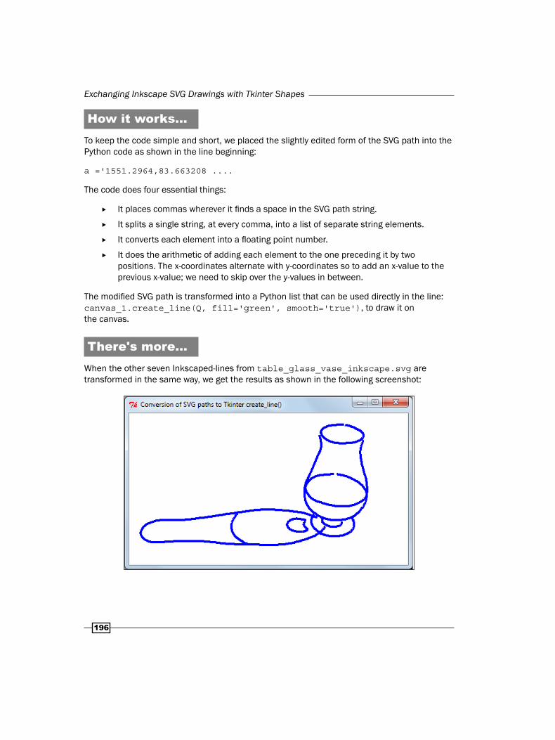
Exchanging Inkscape SVG Drawings with Tkinter Shapes
1�6
How it works...To keep the code simple and short, we placed the slightly edited form of the SVG path into the Python code as shown in the line beginning:
a ='1551.2964,83.663208 ....
The code does four essential things:
It places commas wherever it finds a space in the SVG path string.
It splits a single string, at every comma, into a list of separate string elements.
It converts each element into a floating point number.
It does the arithmetic of adding each element to the one preceding it by two positions. The x-coordinates alternate with y-coordinates so to add an x-value to the previous x-value; we need to skip over the y-values in between.
The modified SVG path is transformed into a Python list that can be used directly in the line: canvas_1.create_line(Q, fill='green', smooth='true'), to draw it on the canvas.
There's more...When the other seven Inkscaped-lines from table_glass_vase_inkscape.svg are transformed in the same way, we get the results as shown in the following screenshot:

Chapter 9
1��
How far should we go with image conversion code?We have tried to keep the code simple and brief. We could have put a lot more effort into automating the slight editing that we did in a text editor to remove the m and place square brackets just inside the quotation marks.
Another way to get SVG paths from raster imagesAnother method of extracting SVG paths from raster images is to use the Path, Trace Bitmap tool followed by the Path, and simplify tools in Inkscape. This method does not work well with complex images such as the one of the transparent glass vase we have used here. It works best with simple black and white images. The Inkscape tool is based on another tool called potrace which has its own interface called potracegui. The problem with the potrace tool is you first have to convert your image into bitmap-type formats. The method we have used in this chapter allows us to make very specific choices about which particular lines we want to use no matter how complex the original image is.


10GUI Construction:
Part 1
In this chapter, we will cover:
Widget configuration
Button focus
The simplest push button with validation
The data entry box
Colored button causing message pop-ups
Complex interaction between buttons
Images on buttons and widget packing geometry
The grid geometry manager and button arrays
Drop-down menus to select from a list
Listbox
Text in a window
IntroductionIn this chapter, we provide recipes for the components that are used to create user interfaces of the graphical kind. These are known as GUI or Graphic User Interface. The commonly-used term for GUI components is Widget. The word Widget has no particular meaning other than "general sort of gadget". If you used the example from Chapter 4, Animation Principles on a color-mixing palette, then you would have used the slider or scale widget which will be explained in this chapter. We will also demonstrate that it is not too difficult to create our own widgets.

GUI Construction: Part 1
200
Widget configuration – a labelWe see here how to change the properties (attributes) of most widgets using its configuration() method.
How to do it...Execute the program shown in the usual way.
# widget_configuration_1.py#>>>>>>>>>>>>>>>>>>>>>>>>>>>>>>>>>>>>>>>>>> from Tkinter import * root = Tk( ) labelfont = ('times', 30, 'bold') widget = Label(root, text='Purple and red mess with your focus') widget.config(bg='red', fg='purple') widget.config(font=labelfont) widget.config(bd=6) widget.config(relief=RAISED)widget.config(height=2, width=40) # lines high, characters widewidget.pack(expand=YES, fill=BOTH)root.mainloop( )
How it works...All widgets have default values such as a gray background, and 12 point font size. Once the code for the creation of a widget has been executed the widget appears on the screen with all its assigned properties. Further down the code, as the program is being executed, the properties of the widget can be changed using the widget.config(attribute=new value) method. The result is shown in the following screenshot:

Chapter 10
201
There's more...Choice is good because it allows us to make our GUIs look good. The downside of this choice is that it allows us to make poor choices. But as the adage goes: poor choices made with intelligence lead to good choices.
If we run this program we will see that the combination of colors made is about the worst that can be made – they interfere with the eye's focusing mechanics because the two colors have different wavelengths and follow slightly different paths on their way to the retina.
Button focusHere we demonstrate the concept of focus, which is easier to show than describe. When there are a group of widgets inside a window, only one widget can react to an event like the click of the mouse button. In this example, the button underneath the mouse cursor has focus and therefore is the one that will respond to a click of the mouse. As the cursor moves over another button, then that button has focus. In this example, the button that has focus changes its color, on a Linux-operating system. On MS Windows, the buttons do not change color but the mouse cursor changes.
How to do it...Execute the program shown in the usual way.
#button_focus_1.py #>>>>>>>>>>>>>>>from Tkinter import * root = Tk()
butn_widget_1 = Button(text='First, RAISED', padx=10, pady=10) butn_widget_1.config(cursor='gumby') butn_widget_1.config(bd=8, relief=RAISED) butn_widget_1.config(bg='dark green', fg='white') butn_widget_1.config(font=('helvetica', 20, 'underline italic')) butn_widget_1.grid(row=1, column = 1)
butn_widget_2 = Button(text='Second, FLAT', padx=10, pady=10) butn_widget_2.config(cursor='circle') butn_widget_2.config(bd=8, relief=FLAT) butn_widget_2.grid(row=1, column = 2)

GUI Construction: Part 1
202
butn_widget_3 = Button(text='Third, SUNKEN', padx=10, pady=10) butn_widget_3.config(cursor='heart') butn_widget_3.config(bd=8, relief=SUNKEN) butn_widget_3.config(bg='dark blue', fg='white') butn_widget_3.config(font=('helvetica', 30, 'underline italic')) butn_widget_3.grid(row=1, column = 3)
butn_widget_4 = Button(text='Fourth, GROOVE', padx=10, pady=10) butn_widget_4.config(cursor='spider') butn_widget_4.config(bd=8, relief=GROOVE) butn_widget_4.config(bg='red', fg='white') butn_widget_4.config(font=('helvetica', 20, 'bold')) butn_widget_4.grid(row=1, column = 4)
butn_widget_5 = Button(text='Fifth RIDGE', padx=10, pady=10) butn_widget_5.config(cursor='pencil') butn_widget_5.config(bd=8, relief=RIDGE) butn_widget_5.config(bg='purple', fg='white') butn_widget_5.grid(row=1, column = 5)
root.mainloop( )
How it works...When we run the preceding code under Linux, we will see that the color of each button change as it acquires focus. The button that has focus is the only one of the group that will react to a left mouse click. Under MS Windows 7, this change of color with focus does not work. Nevertheless, the logic of focus behavior and reaction to mouse events is unaffected.
We have also taken the opportunity to look at the different button border styles available.
There's more...One thing to note in this example is that the size of a button is determined by the font size and amount of text placed on the button.

Chapter 10
203
The simplest push button with validationWe now home in on the simplest example of event processing by means of a callback() function.
The validation referred to previously is any kind of reaction that provides confirmation that our code did what we wanted it to do. When you are developing code experimentally you need some kind of validation at the earliest stage in order build up insight.
How to do it...Copy, save and execute. The result is shown as follows:
# button_1.py#>>>>>>>>>>>>>from Tkinter import * root = Tk()
def callback_1(): # The event processor function print "Someone pushed a button"
# The instantiation (i.e. creation of a specific instance or # realization) of a button.button_1= Button(root, command=callback_1).grid(row=1, column=0) root.mainloop()
How it works...When you push the little button with your mouse pointer, a message will appear on your terminal. The appearance of the message is the vital validation action your program produces.
This simple example demonstrates the fundamental design of all programs that react to user input. Then all you have to do is the following:
Wait for some external event such as the click of a mouse or the tap of a key on the keyboard.
If and when the external event occurs, we must have an event handler function inside our program that specifies what actions must occur. These are often referred to as callback functions.
GUI Construction: Part 1
204
Inside the code, that makes an instance of any widget designed to accept user input, there must always be an option-specifier like command=callback_1 that points to the name of your event-processing function named callback_1 that will do all the things we want it to do when the event occurs. We do not have to use the actual word callback_1 - we could have chosen any word we liked. In this case, the event is the push of a button. All we ask it to do inside the callback() function is to print a message. However, the list of resulting actions initiated by our callback() function can be as long as we like.
There's more...Programming literature often uses the word instantiation, especially with reference to objects in the object-oriented programming context. The word instantiation means to transform some object, which previously only existed as a semi-abstract description, into an actual block of code with a real namespace for its variables that interact with the data and commands inside your program. Python with Tkinter has a pre-defined object called a button. In our preceding program, we instantiate a button named button_1 into existence by the command:
button_1= Button(root, command=callback_1).grid(row=1, column=0)
The description to the right of the equals sign is the pre-existing abstract description taken from a long list of objects inside the Tkinter library. The name button_1 on the left is the name of the instance that will have all of the actual properties that were previously just words in a library. This is like having a file with engineering drawings and assembly instructions for a sports car (the abstract description) and then getting some engineering workshop to actually manufacture an instance of the gleaming steel and chrome speedster. The file with drawings and manufacturing instructions is the equivalent of the object definition in our Python code. The thing with a metallic blue paint job, which you will sit in and drive with the wind in your hair, is an instance of the object.
Buttons behave differently on WindowsThe button in this recipe behaves slightly differently in MS Windows compared to Linux. Windows displays the normal minimize, maximize, close symbols on the top right of the frame containing the button. We close the application by clicking on the top right "X" symbol. In Linux, there is a round button in the top of the frame. When we click this button, a menu opens up with a close command that can end the program.
A data entry boxWe make a GUI that provides a data entry box and a button for handling whatever text is typed into the box.
The Entry widget is a standard Tkinter widget used to enter or display a single line of text.
The button callback() function (event handler) assigns the contents of the textbox to be the value of a variable. All these actions are verified by displaying the value of this variable.

Chapter 10
205
How to do it...Execute the program shown in the normal way.
# entry_box_1.py #>>>>>>>>>>>>>>>from Tkinter import * from Dialog import Dialog root = Tk() root.title("Data Entry Box")
enter_data_1 = Entry(root, bg = "pale green") # Creates a text entry # field enter_data_1.grid(row=1, column=1) enter_data_1.insert(0, "enter text here") # Place text into the box.
def callback_origin(): # Push button event handler. data_inp_1 = enter_data_1.get() # Fetch text from the box.
# Create a label and write the value of 'data_inp_1' to it. # ie. Validate by displaying the newly acquired data as a label on # the frame. label_2_far_right = Label(root, text=data_inp_1) label_2_far_right.grid(row=1, column=3)
# This is button that triggers data transfer from entry box to named# variable 'data_inp_1'. but1= Button(root, text="press to \transfer",command=callback_origin).grid(row=5, column=0)
root.mainloop()
How it works...
A text entry box on its own is not much use. It is like a post box – text can be sent to it or picked up from it.
Dow
nlo
ad fro
m W
ow
! eBook
<w
ww
.wow
ebook.
com
>
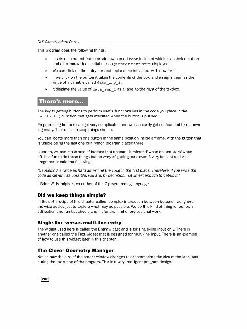
GUI Construction: Part 1
206
This program does the following things:
It sets up a parent frame or window named root inside of which is a labeled button and a textbox with an initial message enter text here displayed.
We can click on the entry box and replace the initial text with new text.
If we click on the button it takes the contents of the box, and assigns them as the value of a variable called data_inp_1.
It displays the value of data_inp_1 as a label to the right of the textbox.
There's more...The key to getting buttons to perform useful functions lies in the code you place in the callback() function that gets executed when the button is pushed.
Programming buttons can get very complicated and we can easily get confounded by our own ingenuity. The rule is to keep things simple.
You can locate more than one button in the same position inside a frame, with the button that is visible being the last one our Python program placed there.
Later on, we can make sets of buttons that appear 'illuminated' when on and 'dark' when off. It is fun to do these things but be wary of getting too clever. A very brilliant and wise programmer said the following:
"Debugging is twice as hard as writing the code in the first place. Therefore, if you write the code as cleverly as possible, you are, by definition, not smart enough to debug it."
—Brian W. Kernighan, co-author of the C programming language.
Did we keep things simple?In the sixth recipe of this chapter called "complex interaction between buttons", we ignore the wise advice just to explore what may be possible. We do this kind of thing for our own edification and fun but should shun it for any kind of professional work.
Single-line versus multi-line entryThe widget used here is called the Entry widget and is for single-line input only. There is another one called the Text widget that is designed for multi-line input. There is an example of how to use this widget later in this chapter.
The Clever Geometry ManagerNotice how the size of the parent window changes to accommodate the size of the label text during the execution of the program. This is a very intelligent program design.

Chapter 10
20�
Colored button causing a message pop-upButtons can be given different visual properties and complex behaviors. Here we create a blue raised button that changes appearance when clicked with a mouse. A message box widget is made to pop up when the button is pushed.
How to do it...Execute the program shown in the normal way.
# button_message_1.py #>>>>>>>>>>>>>>>>>>>from Tkinter import * import tkMessageBox root = Tk() root.title("Message Button")
def callback_button(): tkMessageBox.showinfo( "Certificate of Button Pushery", \ "Are glowing pixels a reality?")
message_button = Button(root, bd=6, # border width relief = RAISED, # raised appearance # to button border bg = "blue", # normal background # color fg = "green", # normal foreground # (text) color font = "Arial 20 bold", text ="Push me", # text on button activebackground = "red", # background when # button is clicked activeforeground = "yellow", # text color when # clicked command = callback_button) # name of event # handler message_button.grid(row=0, column=0)
root.mainloop()

GUI Construction: Part 1
20�
How it works...
What we see now is that buttons are highly customizable, as are many Tkinter widgets. This recipe illustrates another term that you are bound to come across as a GUI programmer and that is the word focus.
Focus is the idea that when there are several widgets on a graphic container only one of them can be given attention or listened to at a time. Each button is programmed to respond to the click of a mouse but when the mouse is clicked, only one button should respond. The widget responding is the one that the program focuses on. In our example, you actually see the focus being given to the button when the mouse pointer moves across it – the focus is used to change the button's coloring in a Linux operating system. It is like the chairman offering the floor to someone wanting to address a meeting group. The aspirant talker can only do so when the chairman offers them the floor (gives them focus). When this happens, everyone else is expected to be quiet and listen courteously.
Complex interaction between buttonsIn this recipe, we show how button actions can be made as complex as we choose by getting a set of three buttons that modify each other.
How to do it...Execute the program shown in the normal way.
# button_interaction_1.py #>>>>>>>>>>>>>>>>>>>>from Tkinter import * root = Tk() root.title("now what?")

Chapter 10
20�
def callback_button_1(): message_button_1.flash() message_button_2["bg"]= "grey" message_button_2.flash() message_button_3.flash() message_button_3["bg"]= "pink" message_button_1["relief"] = SUNKEN message_button_1["text"]= "What have you done?" def callback_button_2(): message_button_2["bg"]= "green" message_button_3["bg"]= "cyan" message_button_1["relief"] = RAISED message_button_1["text"]= "Beware"
def callback_button_3(): message_button_1.destroy() message_button_2.destroy() message_button_3.destroy() root.destroy()
message_button_1 = Button(root, bd=6, relief = RAISED, # Raised # appearance. bg = "blue" # Normal (without # focus) # background # color fg = "green", # Normal (without # focus) # foreground # (text) color font = "Arial 20 bold", text ="Push me first", # Text on button activebackground = "red", # Background when # button has # focus activeforeground = "yellow", #Text with focus command = callback_button_1) # event handler message_button_1.grid(row=0, column=0)
message_button_2 = Button(root, bd=6, relief = SUNKEN,

GUI Construction: Part 1
210
bg = "green", fg = "blue", font = "Arial 20 bold", text ="Now Push me", activebackground = "purple", activeforeground = "yellow", command = callback_button_2) message_button_2.grid(row=1, column=0)
message_button_3 = Button(root, bd=6, relief = SUNKEN, bg = "grey", fg = "blue", font = "Arial 20 bold", text ="kill everything", activebackground = "purple", activeforeground = "yellow", command = callback_button_3) message_button_3.grid(row=2, column=0)
root.mainloop()
How it works...

Chapter 10
211
All the action happens in the event handler (callback()) functions. Every instantiated object, like the buttons used here, has a collection of attributes like color, text, and appearance that can be modified by specifications like: message_button_2["bg"]= "grey"
So what happens is that when button 1 is clicked, button 2 has its background color changed from green to grey.
While it is fun to create very complicated interactive behavior with button actions, it rapidly becomes nearly impossible to keep track of what behavior you want. The more complexity you add, the more unintended behaviors appear. The best advice then is to try to keep things simple.
Images on buttons and button packingBy placing GIF format images onto buttons, we can create any appearance desirable. The images can convey information about the function of the button. Image size has to be taken into account and the geometry manager has to be used thoughtfully.
How to do it...Execute the program shown in exactly the same way as usual.
# image_button_1.py#>>>>>>>>>>>>>>>>>>>>>>>>>>>>>>>>>>>>>>>>>>from Tkinter import *root = Tk()root.title("Image Sized Buttons")
go_image = PhotoImage(file = "/constr/pics1/go_on.gif")fireman_image = PhotoImage(file = "/constr/pics1/fireman_1.gif")winged_lion_image = PhotoImage(file = "/constr/pics1/winged_lion.gif")earth_image = PhotoImage(file = "/constr/pics1/earth.gif")
def callback_go(): print "Go has been pushed to no purpose"
def callback_fireman(): print "A little plastic fireman is wanted"
def callback_lion(): print "A winged lion rampant would look cool on a t-shirt"

GUI Construction: Part 1
212
def callback_earth(): print "Think of the children (and therefore also of their parents)"
btn_go= Button(root, image = go_image, \ command=callback_go ).grid(row=0, column=0)btn_firmean= Button(root, image = fireman_image, \ command=callback_fireman).grid(row=0, column=1)btn_lion= Button(root, image = winged_lion_image, \ command=callback_lion ).grid(row=0, column=2)btn_earth= Button(root, image = earth_image, \ command=callback_earth ).grid(row=0, column=3)
root.mainloop()
How it works...
The thing to notice here is that the grid geometry manager packs all the widgets together as neatly as it can regardless of widget size.
There's more...One of the wonderful thoughts behind the design of Python modules is that their actions should be kind and tolerant. This means that if attributes are coded with unsuitable values then defaults will be selected by the interpreter as at least some choice that is likely to work. This is an enormous boon to coders. If you ever come across one of the inner circle of Python developers they deserve an affectionate hug for this reason alone.

Chapter 10
213
Grid Geometry Manager and button arraysBy placing GIF format images onto buttons, we can create any desired appearance. Image size has to be taken into account and the geometry manager has to be used thoughtfully.
How to do it...Execute the program shown in the normal way.
# button_array_1.py #>>>>>>>>>>>>>>>>> from Tkinter import * root = Tk() root.title("Button Array")
usb = PhotoImage(file = "/constr/pics1/Usbkey_D.gif") galaxy = PhotoImage(file = "/constr/pics1/galaxy_D.gif") alert = PhotoImage(file = "/constr/pics1/alert_D.gif") earth = PhotoImage(file = "/constr/pics1/earth_D.gif")
eye = PhotoImage(file = "/constr/pics1/eye_D.gif") rnd_2 = PhotoImage(file = "/constr/pics1/random_2_D.gif") rnd_3 = PhotoImage(file = "/constr/pics1/random_3_D.gif")
smile = PhotoImage(file = "/constr/pics1/smile_D.gif") vine = PhotoImage(file = "/constr/pics1/vine_D.gif") blueye = PhotoImage(file = "/constr/pics1/blueeye_D.gif") winglion = PhotoImage(file = "/constr/pics1/winglion_D.gif")
def cb_usb(): print "usb" def cb_galaxy(): print "galaxy" def cb_alert(): print "alert" def cb_earth(): print "earth"
def cb_eye(): print "eye" def cb_rnd_2(): print "random_2" def cb_rnd_3(): print "random_3"
def cb_smile(): print "smile" def cb_vine(): print "vine" def cb_blueeye(): print "blueeye" def cb_winglion(): print "winglion"

GUI Construction: Part 1
214
butn_usb = Button(root, image = usb, command=cb_usb \).grid(row=0, column=0) butn_galaxy = Button(root, image = galaxy, command=cb_galaxy).grid(row=1, column=0) butn_alert = Button(root, image = alert, command=cb_alert \).grid(row=2, column=0) butn_earth = Button(root, image = earth, command=cb_earth \).grid(row=3, column=0)
butn_eye = Button(root, image = eye, command=cb_eye \).grid(row=0, column=1, rowspan=2) butn_rnd_2 = Button(root, image = rnd_2, command=cb_rnd_2 \).grid(row=2, column=1) butn_rnd_3 = Button(root, image = rnd_3, command=cb_rnd_3 \).grid(row=3, column=1)
butn_smile = Button(root, image = smile, command=cb_smile \).grid(row=0, column=2, columnspan=2) butn_vine = Button(root, image = vine, command=cb_vine \).grid(row=1, column=2, rowspan=2, columnspan=2) butn_blueye = Button(root, image = blueye, \command=cb_blueeye).grid(row=3, column=2)
butn_winglion= Button(root, image = winglion, command=cb_winglion \).grid(row=3, column=3)
root.mainloop()
How it works...

Chapter 10
215
There are two geometry managers in Tkinter. In this book, we have used the Grid Geometry Manager exclusively up until now because it keeps the level of complexity down and also because it is easy to use and gives you direct control of your interface layout. The other layout geometry manager is called pack and is addressed in the next chapter.
The rules are simple. Our parent window or frame is divided into rows and columns. Row=0 is the first row along the top and column=0 is the first column down the left-hand side. columnspan=2 means that the widget using this attribute sits in the center of two adjacent columns. Note that the button with the vine icon on it sits in the center of four grid regions because it has both columnspan=2 and rowspan=2.
There's more...By changing the grid attributes in this example, you can help yourself acquire an insight to the Grid Geometry Manager. Please experiment with the grid manager for a while – it will pay dividends in your programming endeavors.
Drop-down menus to select from a listHere we use a drop-down menu widget as a way to select one item from a choice of several on offer.
How to do it...Execute the program shown in the usual way. The result is shown in the following screenshot:
# dropdown_1.py# >>>>>>>>>>>>>>>>>>>from Tkinter import *root = Tk()root.title("Drop-down boxes for option selections.")
var = StringVar(root)var.set("drop down menu button")
def grab_and_assign(event): chosen_option = var.get()
Dow
nlo
ad fro
m W
ow
! eBook
<w
ww
.wow
ebook.
com
>

GUI Construction: Part 1
216
label_chosen_variable= Label(root, text=chosen_option) label_chosen_variable.grid(row=1, column=2) print chosen_option
drop_menu = OptionMenu(root, var, "one", "two", "three", "four", \ "meerkat", "12345", "6789", command=grab_and_assign)drop_menu.grid(row=0, column=0)
label_left=Label(root, text="chosen variable= ")label_left.grid(row=1, column=0)
root.mainloop()
How it works...The drop-down menu has its own button. The callback() function that gets called when this button is clicked is named grab_and_assign in this particular recipe and one of the instructions in this event service routine is to assign the value of the menu item selected to the variable chosen_option. The instruction that does this is chosen_option = var.get().
As we did previously, we reassure ourselves that everything works as expected by printing the new value of chosen_option as a label on the parent window.
Listbox variable selectionA listbox is a widget that shows a choice of alternatives in a list form. An item in the list can be selected by clicking the mouse cursor on it.
How to do it...Execute the program shown in the usual way.
# listbox_simple_1.py #>>>>>>>>>>>>>>>>>>from Tkinter import * root = Tk() root.title("Listbox Data Input")
def get_list(event): # Mouse button release callback # Read the listbox selection and put the result in an entry box

Chapter 10
21�
# widget index = listbox1.curselection()[0] # get selected line index seltext = listbox1.get(index) # get the line's text & # assign # to a variable enter_1.delete(0, 50) # delete previous text in # enter_1 otherwise the # entries # append to each other. enter_1.insert(0, seltext) # now display the selected # text
# Create the listbox (note that size is in characters) listbox1 = Listbox(root, width=50, height=6) listbox1.grid(row=0, column=0)
# Fill the listbox with data listbox1.insert(END, "a list entry") for item in ["one has begun", "two is a shoe", "three like a knee", \"four to the door"]: listbox1.insert(END, item)
# use entry widget to display/edit selection enter_1 = Entry(root, width=50, bg='yellow') enter_1.insert(0, 'Click on an item in the listbox') enter_1.grid(row=1, column=0)
# left mouse click on a list item to display selection listbox1.bind('<ButtonRelease-1>', get_list) root.mainloop()
How it works...

GUI Construction: Part 1
21�
A listbox named listbox1 is created and placed inside a Tkinter window. It is populated with five string items using a for loop.
When the mouse cursor is clicked on an item, the function get_list assigns that item as the value of a variable seltext. The value of this variable is displayed in the yellow entry box.
Text in a windowHere is a simple way to place text in a window. There is no provision made to interact with the text.
How to do it...Execute the program shown in the usual way.
# text_in_window_1.py#>>>>>>>>>>>>>>>>>>>>>>>>>>>>>>>>>>>>>>>>>>from Tkinter import *root = Tk()root.title("Text in a window")
text_on_window = Text(root)text_on_window.grid(row=0, column=0)
for i in range(20): text_on_window.insert(END, "Fill an area with some text: line %d\n"\ % i)
root.mainloop()
How it works...A Text widget is created by the Text(root) method and the insert(…) function places the text inside. The END attribute places each new line at the end of the previous one.

11GUI Construction:
Part 2
In this chapter, we will cover:
The Grid Layout Geometry ManagerThe Pack Geometry ManagerRadio buttons to select one from manyCheck buttons (Tick boxes) to select some of manyKeystroke event handlingScrollbarFramesCustom DIY Controller Widgets (a slimmer slider)
IntroductionIn this chapter, we provide more recipes for the Graphical User Interfaces(GUI). The recipes in the previous chapter were devised as basic ways of interacting with your code while it is running. In this chapter we extend these ideas and try to tie them together.
We start by exploring the characteristics of the two layout geometry managers. Throughout this book, up until this chapter we have used the grid manager as it seems to be the one that gives us most control over the appearance of the GUI.
One choice we are forced to make when we write Tkinter code that uses widgets is how we are going to arrange the widgets inside the master widget that contains them. There are two layout geometry managers to choose from: the pack and the grid. The pack manager is the easiest to use until you have your own ideas of how you want the furniture arranged in your house, with furniture and house being useful metaphors for widget and containing widget. The grid manager gives you absolute control of layout.
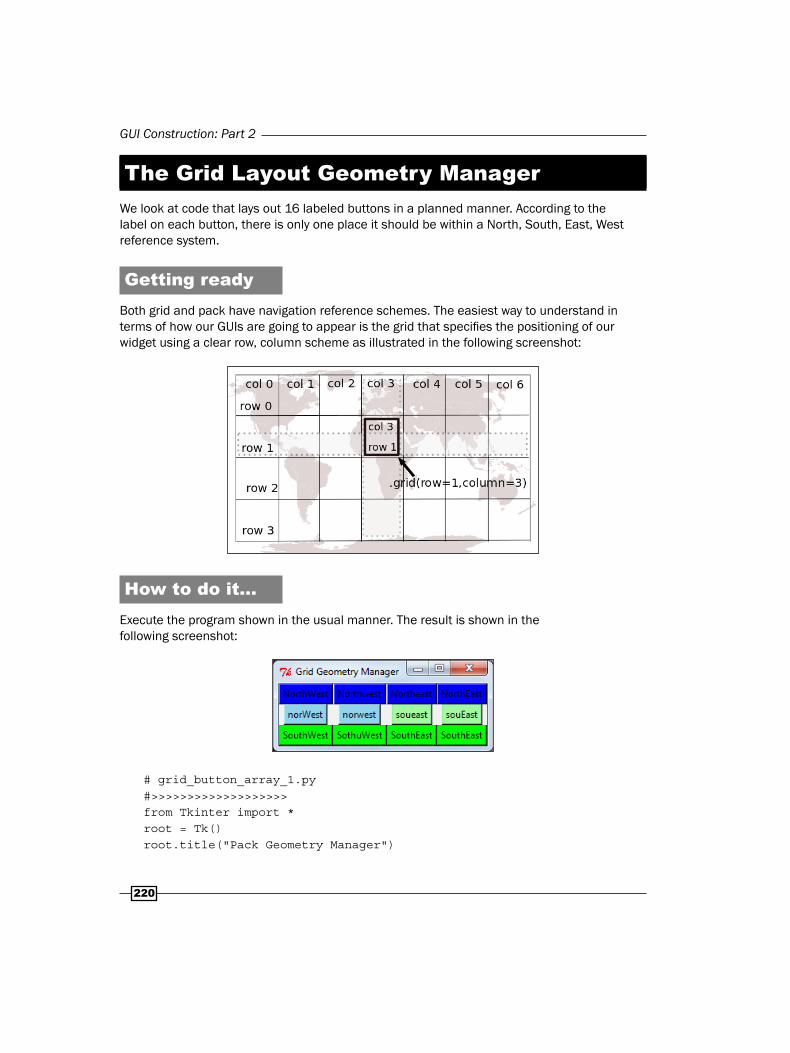
GUI Construction: Part 2
220
The Grid Layout Geometry ManagerWe look at code that lays out 16 labeled buttons in a planned manner. According to the label on each button, there is only one place it should be within a North, South, East, West reference system.
Getting readyBoth grid and pack have navigation reference schemes. The easiest way to understand in terms of how our GUIs are going to appear is the grid that specifies the positioning of our widget using a clear row, column scheme as illustrated in the following screenshot:
How to do it...Execute the program shown in the usual manner. The result is shown in the following screenshot:
# grid_button_array_1.py#>>>>>>>>>>>>>>>>>>>from Tkinter import * root = Tk() root.title("Pack Geometry Manager")

Chapter 11
221
butn_NW = Button(root, bg='blue',text="NorthWest").grid(row=0, \ column=0) butn_NW1 = Button(root, bg='blue',text="Northwest").grid(row=0, \ column=1) butn_NE1 = Button(root, bg='blue',text="Northeast").grid(row=0, \ column=2) butn_NE = Button(root, bg='blue',text="NorthEast").grid(row=0, \ column=3)
butn_N1W = Button(root, bg='sky blue',text="norWest").grid(row=1, \ column=0) butn_N1W1 = Button(root, bg='sky blue',text="norwest").grid(row=1, \ column=1) butn_S1E1 = Button(root, bg='pale green',text="soueast").grid(row=1, column=2) butn_S1E = Button(root, bg='pale green',text="souEast").grid(row=1, column=3)
butn_SW = Button(root, bg='green',text="SouthWest").grid(row=2, \column=0) butn_SW1 = Button(root, bg='green',text="SothuWest").grid(row=2, \ column=1) butn_SE1 = Button(root, bg='green',text="SouthEast").grid(row=2, \ column=2) butn_SE = Button(root, bg='green',text="SouthEast").grid(row=2, \ column=3)
root.mainloop()
How it works...The Grid Layout Manager is explicit in interpreting layout instructions. There is no ambiguity and the results are easy to understand. Fortunately, for us users, one of the entrenched philosophies of the Python language is that wherever possible the interpreter should be kind and forgiving to mildly careless programming. For instance, say for example, we assigned the grid layout of all the buttons to the same address. For example, say we assigned all the buttons as grid(row=5, column=5). The result would be what appeared to be a single button inside the window. In fact, the layout manager would place all the buttons on top of one another, with the first one at the bottom and the last one on top. If we destroyed them one at a time in reverse order we would see this sequence unfolding.
There's more...Just remember that we never mix pack and grid layout managers in the same program. If you do, your program will freeze as each of the managers attempts to obey conflicting instructions.

GUI Construction: Part 2
222
The Pack Geometry ManagerWe attempt to achieve the same result as shown in the previous screenshot without complete success because pack tries to arrange widgets in a single strip. The limited flexibility pack offers is that it allows us to decide where the strip should begin.
Getting readyThe Pack Layout Manager uses a navigator's compass scheme illustrated as follows:
How to do it...Execute the program shown in the usual way. The result is shown in the following screenshot:
# pack_button_array_1.py #>>>>>>>>>>>>>>>>>>>>>>from Tkinter import * root = Tk() root.title("Pack Geometry Manager")
butn_NW = Button(root, bg='blue',text="NorthWest").pack(side=LEFT) butn_NW1 = Button(root, bg='blue',text="Northwest").pack(side=LEFT) butn_NE1 = Button(root, bg='blue',text="Northeast").pack(side=LEFT) butn_NE = Button(root, bg='blue',text="NorthEast").pack(side=LEFT)

Chapter 11
223
butn_N1W = Button(root, bg='sky blue',text="norWest").pack() butn_N1W1 = Button(root, bg='sky blue',text="norwest").pack() butn_S1E1 = Button(root, bg='pale green',text="soueast").pack(side=BOTTOM) butn_S1E = Button(root, bg='pale green',text="souEast").pack(side=BOTTOM)
butn_SW = Button(root, bg='green',text="SouthWest").pack(side=RIGHT) butn_SW1 = Button(root, bg='green',text="SothuWest").pack(side=RIGHT) butn_SE1 = Button(root, bg='green',text="SouthEast").pack(side=RIGHT) butn_SE = Button(root, bg='green',text="SouthEast").pack(side=RIGHT)
root.mainloop()
How it works...The pack geometry packs widgets either in rows or in columns. If we try to do both, the results are difficult to predict as shown in the previous screenshot.
What it does is it starts at one edge, which you may specify, and then just lays the widgets one-by-one next to each other in the same order that they appear in our code. If you do not specify an edge to start on the default is TOP so the widgets will be laid out as a single column.
There are also parameters that specify whether the widget should be padded out to fill available space. We can get this detail from:
http://effbot.org/tkinterbook/pack.htm
Radiobuttons to select one from manyWe use radiobuttons to make one choice from a selection of choices. Each button in the set is linked to the same variable. As one button is left-clicked with the mouse, the value associated with that particular button gets assigned as the value of the variable.
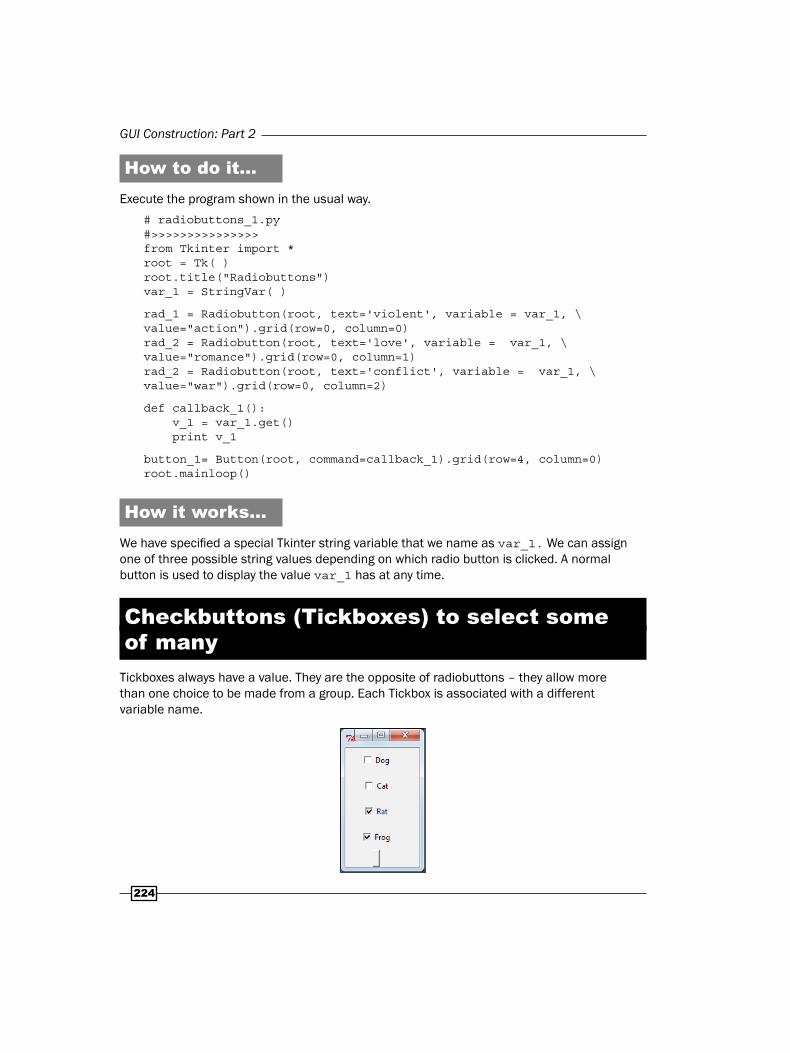
GUI Construction: Part 2
224
How to do it...Execute the program shown in the usual way.
# radiobuttons_1.py #>>>>>>>>>>>>>>>from Tkinter import * root = Tk( ) root.title("Radiobuttons") var_1 = StringVar( )
rad_1 = Radiobutton(root, text='violent', variable = var_1, \ value="action").grid(row=0, column=0) rad_2 = Radiobutton(root, text='love', variable = var_1, \ value="romance").grid(row=0, column=1) rad_2 = Radiobutton(root, text='conflict', variable = var_1, \ value="war").grid(row=0, column=2)
def callback_1(): v_1 = var_1.get() print v_1
button_1= Button(root, command=callback_1).grid(row=4, column=0) root.mainloop()
How it works...We have specified a special Tkinter string variable that we name as var_1. We can assign one of three possible string values depending on which radio button is clicked. A normal button is used to display the value var_1 has at any time.
Checkbuttons (Tickboxes) to select some of many
Tickboxes always have a value. They are the opposite of radiobuttons – they allow more than one choice to be made from a group. Each Tickbox is associated with a different variable name.
Dow
nlo
ad fro
m W
ow
! eBook
<w
ww
.wow
ebook.
com
>

Chapter 11
225
How to do it...Execute the program shown in the usual way.
# checkbox_1.py#>>>>>>>>>>>>>>>>>>>>from Tkinter import * import tkMessageBox root = Tk() root.title("Checkboxes") check_var1 = IntVar() check_var2 = IntVar() check_var3 = StringVar() check_var4 = StringVar()
def change_it(): print "Why do you want to change things?"
Ck_1 = Checkbutton(root, text = "Dog", variable = check_var1, \ command=change_it, \ onvalue = 1, offvalue = 0, height=3, \ width = 10).grid(row=0, column=0) Ck_2 = Checkbutton(root, text = "Cat", variable = check_var2, \ onvalue = 1, offvalue = 0, height=6, \ width = 10).grid(row=1, column=0) Ck_3 = Checkbutton(root, text = "Rat", variable = check_var3, \ onvalue = "fly me", offvalue = "keep walking", \ height=9, \ width = 10).grid(row=2, column=0) Ck_4 = Checkbutton(root, text = "Frog", variable = check_var4, \ onvalue = "to the moon", offvalue = "to Putney road", \height=12, \ width = 10).grid(row=3, column=0)
def callback_1(): v_1 = check_var1.get() v_2 = check_var2.get() v_3 = check_var3.get() v_4 = check_var4.get() print v_1, v_2, v_3, v_4
button_1= Button(root, command=callback_1).grid(row=4, column=0)
root.mainloop()

GUI Construction: Part 2
226
How it works...There are four checkboxes (tickboxes) and therefore four variables. Two are integer and two are strings. Whenever the button at the bottom is clicked, all four values are displayed.
Key-stroke event handlingIn GUI terminology, an Event Handler is a term for a function that executes when an external event such as a key or a mouse being clicked occurs. An equivalent term used in this book, is a callback function. We recognize a callback function because it has the word event as an argument in the function definition.
Here we make an event handler that reacts to key strokes.
How to do it...Execute the program shown in the usual way.
# keypress_1.py #>>>>>>>>>>>>>>>>>>from Tkinter import * root = Tk() root.title("Key symbol Getter") def key_was_pressed(event): print 'keysym=%s' % (event.keysym)
text_1 = Text(root, width=20, height=5, highlightthickness=15) text_1.grid(row=0, column=0)
text_1.focus_set() root.mainloop()
How it works...We have made a textbox to show which key was clicked when a keyboard "event" occurs. We have chosen to display and verify our key presses inside a textbox, which does not react to function key presses. If we used a Label widget instead, we would see the function key displayed as expected. In other words the function event.keypress correctly senses all keystrokes even if they are not represented by normal characters.

Chapter 11
22�
ScrollbarA scrollbar provides a way to move a viewing window across a larger image or text area using a mouse-controlled slider. It can be used with Listboxes, Canvasses, Entry widgets, or Text widgets. In this example, we use a vertical scrollbar to move a GIF image up and down behind a scrollbar's viewing window.
How to do it...A two-way connection needs to be made between the canvas and the scrollbar:
The canvas's yscrollcommand option has to be connected to the vertical scrollbar's .set method, and
The scrollbar's command option has to connected to the canvas's .yview method.
Execute the program shown in the usual way.
scrollbar_1.py#>>>>>>>>>>>>>>>>>>>>>>>>>>>>>>>>>>>>>>>>>>from Tkinter import *
root = Tk()
frame_1 = Frame(root, bd=2, relief=SUNKEN)frame_1.grid(row=0, column=0)
pic_1 = PhotoImage(file="/constr/pics1/table_glass_vase.gif")
yscrollbar = Scrollbar(frame_1, orient=VERTICAL, \ bg="skyblue",activebackground="blue")yscrollbar.grid(row=0, column=1, sticky=N+S)
canvas_1 = Canvas(frame_1, bd=0, scrollregion=(0, 0, 2100, 2000), # The extent of the scrollable area. yscrollcommand=yscrollbar.set, # Link to the # scrollbar.)canvas_1.grid(row=0, column=0)canvas_1.create_image(0 ,0 ,anchor=NW, image= pic_1)
yscrollbar.config(command=canvas_1.yview) # Link to the #canvas.mainloop()
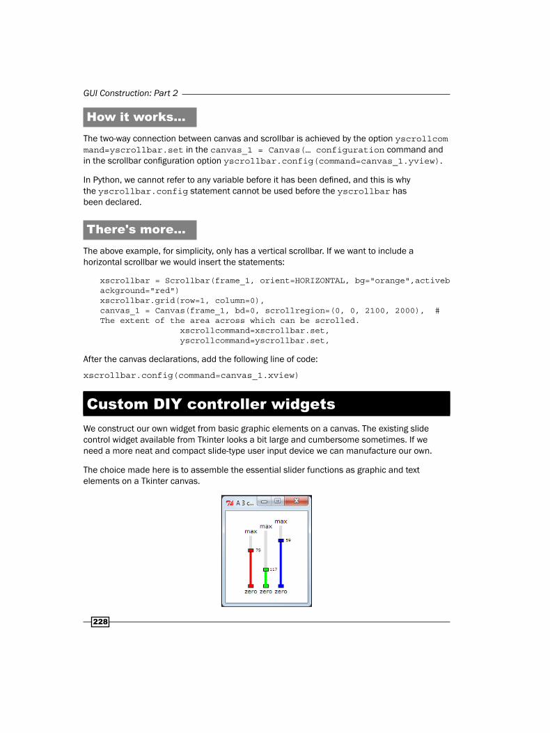
GUI Construction: Part 2
22�
How it works...The two-way connection between canvas and scrollbar is achieved by the option yscrollcommand=yscrollbar.set in the canvas_1 = Canvas(… configuration command and in the scrollbar configuration option yscrollbar.config(command=canvas_1.yview).
In Python, we cannot refer to any variable before it has been defined, and this is why the yscrollbar.config statement cannot be used before the yscrollbar has been declared.
There's more...The above example, for simplicity, only has a vertical scrollbar. If we want to include a horizontal scrollbar we would insert the statements:
xscrollbar = Scrollbar(frame_1, orient=HORIZONTAL, bg="orange",activebackground="red")xscrollbar.grid(row=1, column=0),canvas_1 = Canvas(frame_1, bd=0, scrollregion=(0, 0, 2100, 2000), # The extent of the area across which can be scrolled. xscrollcommand=xscrollbar.set, yscrollcommand=yscrollbar.set,
After the canvas declarations, add the following line of code:
xscrollbar.config(command=canvas_1.xview)
Custom DIY controller widgetsWe construct our own widget from basic graphic elements on a canvas. The existing slide control widget available from Tkinter looks a bit large and cumbersome sometimes. If we need a more neat and compact slide-type user input device we can manufacture our own.
The choice made here is to assemble the essential slider functions as graphic and text elements on a Tkinter canvas.

Chapter 11
22�
How to do it...What we see in the following code are three similar groups of code separated by double lines and a callback function that focuses on one of the three segments depending on the value of a variable named focus_flag. Execute the program shown in the usual way.
# mini_slider_widget_1.py #>>>>>>>>>>>>>>>>>>>>from Tkinter import * import math root = Tk() root.title("A 3 color linear slider control gadget") cw = 200 # canvas width ch = 200 # canvas height chart_1 = Canvas(root, width=cw, height=ch, background="#ffffff") chart_1.grid(row=1, column=1)
#============================================# Mini slider canvas widget focus_flag = 0 # 0-> uncommited, 1 -> slider #1, 2 -> slider #2 etc. x_1 = 50 # Position of slider #1 base. y_1 = 150 x_2 = 80 # Position of slider #2 base. y_2 = 150 x_3 = 110 # Position of slider #3 base. y_3 = 150
length_1 = 100 # Length of slider #1 (pixels) - constant. length_2 = 110 length_3 = 120 slide_1 = y_1 # Position of slider handle #1 - variable. slide_2 = y_2 slide_3 = y_3 #============================================== def separation(x_now, y_now, x_dot, y_dot): # distance # measurement # Distance to points - used to find out if the mouse clicked # inside a circle sum_squares = (x_now - x_dot)**2 + (y_now -y_dot)**2 distance= int(math.sqrt(sum_squares)) # get #pythagorean distance return( distance)

GUI Construction: Part 2
230
#============================================== def canv_slider(xn, yn, length, kula): # Draw the background slider gadgets. y_top = yn -length chart_1.create_line(xn, yn, xn, y_top, fill="gainsboro", width = 6) chart_1.create_rectangle(xn - 5, yn -3, xn + 5, yn + 3, fill=kula, tag="knob_active") chart_1.create_text(xn, yn + 10, text='zero',font=('verdana', 8)) chart_1.create_text(xn, y_top - 10, text='max',font=('verdana', 8))
canv_slider(x_1, y_1, length_1, "red") canv_slider(x_2, y_2, length_2, "green") canv_slider(x_3, y_3, length_3, "blue") #============================================== def dyn_slider(xn, yn, slide_val, kula, tagn): # Draw the dynamic slider position. chart_1.delete(tagn) chart_1.create_line(xn, yn, xn, slide_val, fill=kula, width=4, tag =tagn) chart_1.create_rectangle(xn - 5, slide_val -3 , xn + 5,slide_val + 3, fill=kula, tag=tagn) chart_1.create_text(xn + 15, slide_val, text=str(slide_val), font=('verdana', 6),tag =tagn) #============================================== def callback_1(event): # LEFT CLICK event processor. global x_1, y_1, x_2, y_2, x_3, y_3, focus_flag global slide_1, slide_2, slide_3 # Measure distances to identify which point has been clicked on. d1 = separation(event.x, event.y, x_1, slide_1) d2 = separation(event.x, event.y, x_2, slide_2) d3 = separation(event.x, event.y, x_3, slide_3) if d1 <= 5: focus_flag = 1 if d2 <= 5: focus_flag = 2 if d3 <= 5: focus_flag = 3
def callback_2(event): # LEFT DRAG event processor. global length_1, length_2, length_3 global x_1, y_1, x_2, y_2, x_3, y_3, focus_flag global slide_1, slide_2, slide_3
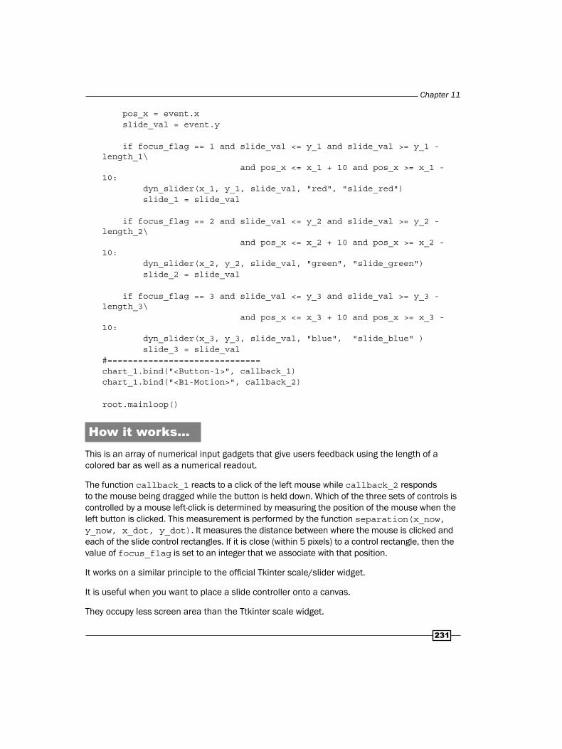
Chapter 11
231
pos_x = event.x slide_val = event.y
if focus_flag == 1 and slide_val <= y_1 and slide_val >= y_1 - length_1\ and pos_x <= x_1 + 10 and pos_x >= x_1 - 10: dyn_slider(x_1, y_1, slide_val, "red", "slide_red") slide_1 = slide_val
if focus_flag == 2 and slide_val <= y_2 and slide_val >= y_2 - length_2\ and pos_x <= x_2 + 10 and pos_x >= x_2 - 10: dyn_slider(x_2, y_2, slide_val, "green", "slide_green") slide_2 = slide_val
if focus_flag == 3 and slide_val <= y_3 and slide_val >= y_3 - length_3\ and pos_x <= x_3 + 10 and pos_x >= x_3 - 10: dyn_slider(x_3, y_3, slide_val, "blue", "slide_blue" ) slide_3 = slide_val #============================== chart_1.bind("<Button-1>", callback_1) chart_1.bind("<B1-Motion>", callback_2)
root.mainloop()
How it works...This is an array of numerical input gadgets that give users feedback using the length of a colored bar as well as a numerical readout.
The function callback_1 reacts to a click of the left mouse while callback_2 responds to the mouse being dragged while the button is held down. Which of the three sets of controls is controlled by a mouse left-click is determined by measuring the position of the mouse when the left button is clicked. This measurement is performed by the function separation(x_now, y_now, x_dot, y_dot). It measures the distance between where the mouse is clicked and each of the slide control rectangles. If it is close (within 5 pixels) to a control rectangle, then the value of focus_flag is set to an integer that we associate with that position.
It works on a similar principle to the official Tkinter scale/slider widget.
It is useful when you want to place a slide controller onto a canvas.
They occupy less screen area than the Ttkinter scale widget.

GUI Construction: Part 2
232
There's more...If we need only one canvas slider widget and not three it is a simple matter to comment-out or delete any lines of code dealing with two of the widgets.
Organizing widgets inside framesWe use Tkinter frames to group bunches of related widgets together. When we have done this, we only have to think about how we want the frames arranged because their contents are already taken care of.
How to do it...Execute the program shown in the usual way.
# frame_1.py #>>>>>>>>>>>>>>from Tkinter import * root = Tk() root.config(bg="black")root.title("It's a Frame-up")
#================================================ # frame_1 and her motley little family frame_1 = Frame(root, bg="red", border = 4, relief="raised") frame_1.grid(row=0, column=0, columnspan=2)

Chapter 11
233
redbutton_1 = Button(frame_1, text="Red",bg ="orange", fg="red") redbutton_1.grid(row=0, column=1)
greenbutton_1 = Button(frame_1, text="Brown",bg ="pink", fg="brown") greenbutton_1.grid(row=1, column=2)
bluebutton_1 = Button(frame_1, text="Blue",bg ="yellow", fg="blue") bluebutton_1.grid(row=0, column=3) #================================================ # frame _2 and her neat blue homeframe_2 = Frame(root, bg="blue", border = 10, relief="sunken") frame_2.grid(row=1, column=0)
redbutton_2 = Button(frame_2, text="Green",bg ="brown", fg="green") redbutton_2.grid(row=0, column=1)
greenbutton_2 = Button(frame_2, text="Brown",bg ="green", fg="brown") greenbutton_2.grid(row=2, column=2)
bluebutton_2 = Button(frame_2, text="Pink",bg ="gray", fg="black") bluebutton_2.grid(row=3, column=3)
#================================================ # frame_3 with her friendly green homeframe_3 = Frame(root, bg="green", border = 20, relief="groove") frame_3.grid(row=1, column=1)
redbutton_3 = Button(frame_3, text="Purple",bg ="white", fg="red") redbutton_3.grid(row=0, column=3)
greenbutton_3 = Button(frame_3, text="Violet",bg ="cyan", fg="violet") greenbutton_3.grid(row=2, column=2)
bluebutton_3 = Button(frame_3, text="Cyan",bg ="purple", fg="blue") bluebutton_3.grid(row=3, column=0)
root.mainloop()

GUI Construction: Part 2
234
How it works...The position of frames is specified relative to the "root" window.
Inside each frame, the widgets that belong to it are arranged without reference to anything outside that frame.
For instance, the specification redbutton_1.grid(row=0, column=1) places the red_button in row=0 and column=1 in the grid geometry that is the universe of the red frame – frame_1. The red button is completely unaware of the world outside her frame.
There's more...For the first time we have changed the background color of the root Tkinter window from the default gray one to black.
Dow
nlo
ad fro
m W
ow
! eBook
<w
ww
.wow
ebook.
com
>

Quick tips for running Python programs in Microsoft Windows
Running Python programs in Microsoft Windows
In a Linux-operating system, Python is usually already installed. It already has Tkinter, math, and many other libraries installed. You do not have to modify any system search path variables like Path to run Python.
Microsoft Windows may throw up some obstacles but it is not too difficult to overcome them. The Python Windows installer will install everything it needs in a Windows directory C:\Python27, if it is version 2.7. Python version 2.6 would get stored in C:\Python26.
Where will we find the windows installer?We will find it at www.python.org/download/. When the www.python.org/download/ page opens up, select Python 2.7 Windows installer (Windows binary – does not include source).
This will download a file named Python-2.7.msi into our windows Downloads folder. We just have to double-click on this file and Python version 2.7 will install itself onto our system at C:\Python27.

Quick tips for running Python programs in Microsoft Windows
236
Do we have to use Python version 2.�?No, the code in this book should work on Python versions 2.4, 2.5, 2.6, and 2.7. It has been run by various people on these versions. It will not run on Python version 3.0 and higher without changes required by the new Python syntax. For instance, print has to be changed to print (stuff-to-be printed).
Why do we get "python is not recognized…"?This happens because the Windows operating system does not know where to find Python when you type python into a command window as shown in the following screenshot:
There are three ways around this problem:
1. Type in the full pathname for both python and the target program we want to run. In this example, we have used the python program named entry_box_1.py. It has been stored inside a folder named constr as described in the first example Running a Shortest Python Program in the first chapter. The following screenshot shows the command-line dialog. george is the name of the user logged into Windows.

Appendix
23�
2. Work inside the Python27 folder. What we do is cd.. and cd.. again. Then cd into folder Python27. Then we can just type python \constr\entry_box_1.py into the command-line as shown in the following screenshot:
3. Change the Windows system variable that informs Windows where to search for executable files. We do this by typing set PATH=%PATH%;C:\Python27 into the command-line window. From now on, we can just type python \constr\entry_box_.py from within any folder. The dialog that achieves this is shown in the following screenshot:


��9
IndexAalignment property, text 49, 52animation
about 57ball, bouncing 65, 67ball, bouncing in gravity field 67-69ball-to-ball collision rebounds 73-76colored disk, creating 58, 59colored disk, shifting 58, 59completing, draw-move-pause-erase cycles
used 62, 63digital flower example 82-84image sequence, creating for 137, 138lines, rotating 76-78mid-air collision 72-76multiple objects, moving 63-65simulation flaws, eliminating 70-72static shifting 58, 59time controlled shifting 60, 61trajectory tracing, on multiple line rotations
78-81working 57
animdelay() function 145ANTIALIAS filters 122Apteryx image
animating 145-149arc
circle, drawing from 34, 35arrows
lines, drawing with 20, 21attributes
defining 115
Bbackground image
making endless 164, 166ball
bouncing 65, 67bouncing, in gravity field 67-69static shifting 58, 59time controlled shifting 59-61
bandList specifier 133BICUBIC filters 122BILINEAR filters 122blue raised button
creating 207, 208BMP image 116button arrays
GIF format images, placing 211-215button focus
concept, demonstrating 201, 202buttons
behaving, differently on Windows 204
Ccanvas
text, placing on 43, 44, 47canvas() method 16canvas.after(milliseconds) function 59canvas.after(your-chosen-milliseconds)
method 61canvas.delete(ALL) method 63canvas.update() function 59checkbuttons
about 224example 225working 226
��0
choice 201circle
about 33drawing, from arc 34, 35drawing, from oval 32, 33
Clever Geometry Manager 206colored disk
creating 58, 59shifting 58, 59
color lists 89color mixing 97color mixing palette 101colors
altering, in images 125, 126rectangular color swatches chart 86-88similar colors, eliminating 86-88specifying, ways 90
color tuplesconverting, to Tkinter Hex compatible
specifiers 91compiled executable
creating, under Linux 11, 12creating, under MS Windows 11, 12
complicated shapesdrawing, mouse clicks used 173, 174
composite imagemaking 132, 133
concentric squaresdrawing 30, 32
configuration() methodabout 200using 200
continuous band of imagespreparing 162, 163
coordinate system 17create-rectangle() method 30create_arc() method 34, 35create_line() method 11, 18create_line(x0,y0 …) function 186create_oval() method 32create_polygon() method 37create_text() method 45cx_Freeze program
about 11downloading, URL 11
Ddashed line
drawing 18, 19data
adding, to existing file 170, 171retrieving, from disk 172, 173writing, to file 169writing, to multiple files 169, 170
data entry boxabout 204working 206
data filecreating, on disk 168reading 168, 169
debugging 206detect_Wall_Collision() function 67diplomat walking at palace recipe 152-156disk
data, retrieving from 172, 173data file, creating 168Tkinter-drawing shape, saving 171, 172
draw-move-pause-erase cyclesusing, in animation 62, 63
drop-down menu widgetusing 215, 216
EEDGE_ENHANCE filter 136ellipse
three arc ellipse, drawing 35, 36endcaps
lines, drawing with 20, 21Entry widget 204eval() function 172, 173event handler
about 226example 226working 226
event processingexample 203, 204
Ffile image formats
BMP 116GIF 116

��1
JPEG 116PNG 116TIFF 116
filter effectsdemonstrating, on images 135, 136
filtersabout 122ANTIALIAS 122BICUBIC 122BILINEAR 122
fontsavailability, verifying on computer 54, 55
fonts_available.sort() function 55
Ggedit text editor 6get_list function 218GIF beach ball image
animating 140, 141GIF format images
placing, on button arrays 211-215GIF images
about 114-116making, with transparent background 149-
152GIMP
about 149GIF images. making with transparent
backgrounds 149-152URL 149
GNU Image Manipulation Program. See GIMPgraded color wheel
example 106-109graphics 16Graphic User Interface. See GUIgrid geometry manager 215Grid Layout Geometry Manager
about 220example 220, 221working 221
GUI 199
Hhexadecimal color specification scheme
color shades series, preparing 91-93
Iimage
blending 130, 131blending, by percentages 131, 132color band, isolating 124, 125colors, altering 125, 126composite image, making 132, 133converting, to other format 118, 120filter effects, demonstrating on 135, 136opening, in different format 117, 118re-sizing, with correct aspect ratio 123, 124rolling 134rotating, in plane 120, 121saving, in different format 117, 118sequence, creating for animation 137, 138size, altering 121, 122transformation effects, applying 134
Image.size() functionabout 123working 124
Image.split() function 125image_open() function 114image file
opening 114-116ImageFilter module 135image formats, Python 114Image module
about 114working 115, 116
image shapetracing, InkSpace used 189-193
Inkscapeabout 180downloading, URL 186drawings, encoding 186, 187image shape, tracing 189-193
insert(…) function 218instantiation 204intricate shapes
drawing 24-26Isaac Newton's Color Wheel 96item
selecting, from listbox 216-218
JJPEG image 116
���
Llines
drawing, with arrows 20, 21drawing, with endcaps 20, 21line with curved bend, drawing 23rotating 76-78
Linuxcompiled executable, creating 11, 12
listboxabout 216item, selecting from 216-218
Mmammal and bird leg motions
combining 156-159mask image
using 132, 133math module 145message box widget 207Microsoft Windows
Python programs, running 235mouse-controlled slider positions
using 130mouse-drawn shape
retrieving 174-176storing 174-176
mouse-shaped editorabout 177working 180
mouse events 181, 183moving band of images
preparing 160, 162MS Windows
compiled executable, creating 11, 12multi line entry
versus single line entry 206multiple line rotations
trajectory tracing 78-81multiple objects
moving 63-65
Nnamed colors 86newline character 169
OOpenClipArt
URL 186oval
circle, drawing from 32, 33overlapping rectangles
drawing 28-30
PPack Geometry Manager
about 215, 222example 222, 223working 223
pair of walking legscreating, vector graphics used 141-145
pen toolZ shape, drawing with 186, 187
pickle method 172PIL
about 114, 140downloading, URL 114
pixel 10PNG image 116polygons
drawing 36potrace 197potracegui 197print command
about 8, 44working 9
propertieschanging, for widgets 200
push buttonwith validation 203, 204
py2exe program 13Python
image formats 114Python 2.7 Windows installer
URL, for downloading 235Python Imaging Library. See PILpython is not recognized… problem
about 236solving, ways 236, 237
Python modules 7

���
Python programrunning 6, 7running, in Microsoft Windows 235Tkinter command, executing 9, 10
Rradiobuttons
about 223example 224working 224
raster imagesabout 113, 139SVG paths, extracting from 197
rectangledrawing 27, 28
SScaled Vector Graphics. See SVGscrollbar
about 227example 227working 228
set of three buttonsmodifying, one another 208-211
SHARPEN filter 136simulation flaws
eliminating 70-72single line entry
versus multi line entry 206size
altering, for image 121, 122slide control 127slider widgets 105spline fitting 24star polygon
drawing 37, 38stars
re-positioning 39, 40resizing 39, 40
straight linedrawing, on canvas 17, 18
SVGabout 23, 180, 185code 189directives 188
SVG code 189SVG directives 188SVG drawing
about 186structure 186, 187
SVG pathconverting, into Tkinter Line 194-196extracting, from raster images 197
Ttext
aligning 49, 52color attribute 45, 46font type attribute 45, 46placing, in window 218placing, on canvas 43, 44, 47placing, position specifiers used 46size attribute 45, 46
Text(root) method 218tickboxes. See checkbuttonsTIFF image 116tkFont module 55Tkinter
about 85robustness 61
Tkinter-drawing shapesaving, to disk 171, 172
Tkinter commandexecuting, inside Python program 9, 10
Tkintercreate_line() function 194Tkinter frames
widgets, organizing 232, 234Tkinter Hex compatible specifiers
color tuples, converting to 91Tkinter Line
SVG path, converting to 194-196tool
constructing, for desirable color mix 127-130trigonometry
about 141using 145
two segment linedrawing 22
Dow
nlo
ad fro
m W
ow
! eBook
<w
ww
.wow
ebook.
com
>

���
Vvector images
about 113, 139pair of walking legs, creating 141-145
Wwedge-shaped segment
creating 94, 95widget.config(attribute=new value) method
200
widgetsabout 199constructing 228-231organizing, in frames 232, 234properties, changing 200
windowtext, placing on 218
World Wide Web Consortium 185
ZZ shape
drawing, with pen tool 186, 187

Thank you for buying
Python 2.6 Graphics Cookbook
About Packt PublishingPackt, pronounced 'packed', published its first book "Mastering phpMyAdmin for Effective MySQL Management" in April 2004 and subsequently continued to specialize in publishing highly focused books on specific technologies and solutions.
Our books and publications share the experiences of your fellow IT professionals in adapting and customizing today's systems, applications, and frameworks. Our solution based books give you the knowledge and power to customize the software and technologies you're using to get the job done. Packt books are more specific and less general than the IT books you have seen in the past. Our unique business model allows us to bring you more focused information, giving you more of what you need to know, and less of what you don't.
Packt is a modern, yet unique publishing company, which focuses on producing quality, cutting-edge books for communities of developers, administrators, and newbies alike. For more information, please visit our website: www.packtpub.com.
About Packt Open SourceIn 2010, Packt launched two new brands, Packt Open Source and Packt Enterprise, in order to continue its focus on specialization. This book is part of the Packt Open Source brand, home to books published on software built around Open Source licenses, and offering information to anybody from advanced developers to budding web designers. The Open Source brand also runs Packt's Open Source Royalty Scheme, by which Packt gives a royalty to each Open Source project about whose software a book is sold.
Writing for PacktWe welcome all inquiries from people who are interested in authoring. Book proposals should be sent to [email protected]. If your book idea is still at an early stage and you would like to discuss it first before writing a formal book proposal, contact us; one of our commissioning editors will get in touch with you.
We're not just looking for published authors; if you have strong technical skills but no writing experience, our experienced editors can help you develop a writing career, or simply get some additional reward for your expertise.
Python MultimediaISBN: 978-1-849510-16-5 Paperback: 292 pages
Learn how to develop Multimedia applications using Python with this practical step-by-step guide
1. Use Python Imaging Library for digital image processing.
2. Create exciting 2D cartoon characters using Pyglet multimedia framework
3. Create GUI-based audio and video players using QT Phonon framework.
4. Get to grips with the primer on GStreamer multimedia framework and use this API for audio and video processing.
Matplotlib for Python DevelopersISBN: 978-1-847197-90-0 Paperback: 308 pages
Build remarkable publication-quality plots the easy way
1. Create high quality 2D plots by using Matplotlib productively
2. Incremental introduction to Matplotlib, from the ground up to advanced levels
3. Embed Matplotlib in GTK+, Qt, and wxWidgets applications as well as web sites to utilize them in Python applications
4. Deploy Matplotlib in web applications and expose it on the Web using popular web frameworks such as Pylons and Django
Please check www.PacktPub.com for information on our titles

Python 3 Object Oriented ProgrammingISBN: 978-1-849511-26-1 Paperback: 404 pages
Harness the power of Python 3 objects
1. Learn how to do Object Oriented Programming in Python using this step-by-step tutorial
2. Design public interfaces using abstraction, encapsulation, and information hiding
3. Turn your designs into working software by studying the Python syntax
4. Raise, handle, define, and manipulate exceptions using special error objects
Python Testing: Beginner’s GuideISBN: 978-1-847198-84-6 Paperback: 256 pages
An easy and convenient approach to testing your powerful Python projects
1. Covers everything you need to test your code in Python
2. Easiest and enjoyable approach to learn Python testing
3. Write, execute, and understand the result of tests in the unit test framework
4. Packed with step-by-step examples and clear explanations
Please check www.PacktPub.com for information on our titles

MySQL for PythonISBN: 978-1-849510-18-9 Paperback: 440 pages
Integrate the flexibility of Python and the power of MySQL to boost the productivity of your Python applications
1. Implement the outstanding features of Python’s MySQL library to their full potential
2. See how to make MySQL take the processing burden from your programs
3. Learn how to employ Python with MySQL to power your websites and desktop applications
4. Apply your knowledge of MySQL and Python to real-world problems instead of hypothetical scenarios
Python Text Processing with NLTK �.0 CookbookISBN: 978-1-84951-360-9 Paperback: 272 pages
Use Python’s NLTK suite of libraries to maximize your Natural Language Processing capabilities
1. Quickly get to grips with Natural Language Processing – with Text Analysis, Text Mining, and beyond
2. Learn how machines and crawlers interpret and process natural languages
3. Easily work with huge amounts of data and learn how to handle distributed processing
4. Part of Packt’s Cookbook series: Each recipe is a carefully organized sequence of instructions to complete the task as efficiently as possible
Please check www.PacktPub.com for information on our titles
Expert Python ProgrammingISBN: 978-1-847194-94-7 Paperback: 372 pages
Best practices for designing, coding, and distributing your Python software
1. Learn Python development best practices from an expert, with detailed coverage of naming and coding convention
2. Apply object-oriented principles, design patterns, and advanced syntax tricks
3. Manage your code with distributed version control
4. Profile and optimize your code
Python Geo-Spatial DevelopmentISBN: 978-1-84951-154-4 Paperback: 480 pages
Build a complete and sophisticated mapping application from scratch using Python tools for GIS development
1. Build applications for GIS development using Python
2. Analyze and visualize Geo-Spatial data
3. Comprehensive coverage of key GIS concepts
4. Recommended best practices for storing spatial data in a database
5. Draw maps, place data points onto a map, and interact with maps
Please check www.PacktPub.com for information on our titles
Dow
nlo
ad fro
m W
ow
! eBook
<w
ww
.wow
ebook.
com
>