the financial markets and wealth effects on …
TRANSCRIPT
UNIVERSITA' DEGLI STUDI DI TRENTO - DIPARTIMENTO DI ECONOMIA ___________________________________________________________________
__________
THE FINANCIAL MARKETS AND WEALTH EFFECTS ON
CONSUMPTION AN EXPERIMENTAL ANALYSIS
Matteo Ploner
_________________________________________________________
Discussion Paper No. 6, 2003

The Discussion Paper series provides a means for circulating preliminary research results by staff of or visitors to the Department. Its purpose is to stimulate discussion prior to the publication of papers. Requests for copies of Discussion Papers and address changes should be sent to: Prof. Andrea Leonardi Dipartimento di Economia Università degli Studi Via Inama 5 38100 TRENTO ITALY
2

THE FINANCIAL MARKETS AND WEALTH EFFECTS ON CONSUMPTION
AN EXPERIMENTAL ANALYSIS∗
Matteo Ploner
S.Anna School for Advanced Studies, Pisa, Italy
3
∗ I am grateful for the support and for the useful comments received from Professor Roberto Tamborini. The experiment has benefited from the comments of Professor Luigi Mittone and of all the staff at CEEL (Computable and Experimental Economics Labotatory) of the University of Trento, Italy. These people and oll the others who enriched this paper with their ideas are not responsible for the remaining errors.

ABSTRACT
The paper investigates the effects exerted by the ownership of quoted equities on intertemporal wealth allocation. To this end, it reports an experiment conducted with human subjects. The fact that an increasing share of household balances is allocated to equities raises numerous questions on the nature and magnitude of so-called ‘wealth effects’. The traditional theories are based on the assumption of perfect rational agents and do not consider wealth effects in detail. The empirical literature on the topic is heterogeneous and does not give a uniform description of such effects. The decision to work with experimental tools was prompted by the idea that this approach would shed light on the behaviour of subjects asked to decide on simulated consumption/saving decisions. The neutral position taken up with respect to the traditional theory when designing the experiment enabled us to compare the outcomes of the laboratory experiment against the theoretical findings of Hall's (1978) model, which describes a Random Walk in consumption. This analysis yielded a much more complex picture than would have been obtained in the perfect rationality framework which supports the traditional theories of life cycle-permanent income. In trying to understand and give a theoretical framework to the behaviour observed in the laboratory, we consider models taken from both the economic and the psychological literature. The analysis furnishes interesting insights, which are described and considered as future directions for research.
4

INTRODUCTION
Decisions on the intertemporal allocation of wealth constitute one of the building blocks of modern economic theory. This field of inquiry comprises models that are widely accepted and appear in all the economics textbooks (life cycle, permanent income). There are also numerous empirical studies on time series. The contradictions apparent in the empirical literature, and the criticisms brought against the strong rationality requirements and computational capacity pretensions of the traditional theories, prompted us to tackle the problem using an alternative approach open to the contributions of both psychological and economic studies, the intention being to reconcile theory with the real computational, motivational and decisional factors of the human mind. Within this general framework, the paper describes an experiment conducted with human subjects in order to observe how decisions regarding the intertemporal allocation of wealth are taken in a controlled environment.
The experiment comprised three different sessions, during which each subject working independently from the others. The starting point of each session was a given amount of wealth which had to be changed into consumption within a given and known time horizon. At the end of this time interval, the subject was rewarded with an amount of real money proportional to the consumption recorded in the three sessions. The sessions were of increasing difficulty, and in the last one the subjects were at risk of having insufficient wealth to "survive" until the end.
In the main sessions of the experiment (the last two), we investigated the behaviour of individuals whose portfolios were stochastic determined in value – as are the portfolios of those who possess equities. The number of households that allocate their wealth in financial markets is increasing, and this feature, together with sharp changes in stock values like those observed in the 1990s, may generate unexpected effects on aggregate consumption.
Although experimental analysis is becoming increasingly frequent in economics, there are still topics that are not appropriately considered in this framework. A case in point is decisions regarding the intertemporal allocation of wealth. Other experimental studies on intertemporal allocation (Hey, 1998; Anderhub-Guth-Müller-Strobel, 2001) have shown the difficulties encountered by researchers when seeking to reproduce the intertemporal context in a laboratory. In consideration of previous studies on the matter, we tried to impose the least constraints possible on the subjects’ decisions. We assumed only that individuals obey the monotonicity axiom and hence prefer a larger 5

reward to a smaller one. We also adopted a deterministic and known life horizon so that the subjects were not given an excessively burdensome computational task.
The first section of the paper gives a short description of wealth effects, taking consideration of the point of view adopted by the standard theories and empirical studies on time series. Section 2 briefly illustrates the behavioural implications of consumption/saving decisions, referring to specific models taken from both the economic and psychological literature. Section 3 describes the experiment and its theoretical underpinnings. Section 4 illustrates the experimental design and gives some technical details. Section 5 continues the presentation, focusing on the three sections which constituted the experiment. Section 6 analyzes the data collected, while the final section verifies the behavioral hypothesis set out in Section 2 against the outcomes of the experiment. On the basis of this analysis, some possible future directions for research are described.
1. THE WEALTH EFFECTS ON CONSUMPTION
Quoted stocks are becoming an increasing component of the wealth of households. This is due both to the increase in direct ownership and to the spread of pension wealth programmes. If the value of owned stocks increases (decreases), there will be a direct effect on the intertemporal budget constraint, which will expand or diminish respectively. Because decisions about current consumption or saving are based on this budget, a change will be observed in the strategy of intertemporal allocation. The mechanism described, which starts from the financial markets and leads to the decision whether to save or consume, is called the wealth effect. The effect is then termed ‘direct’ because it works on the budget constraint. The situation in which the financial markets influence consumption as a proxy for future economic activity is called the ‘indirect’ effect.
The standard theories on intertemporal wealth allocation (permanent income-life cycle) do not discriminate among variations in wealth by nature and source. The variation recorded in consumption is determined only by the marginal propensity to consume. This coefficient is independent of wealth and is defined by the interest rate and by the residual life perspectives. This result is a derivation of the strong assumption of the perfect rationality of agents. Individuals are supposed not to be bounded in their computational capacities for intertemporal planning, nor in their amount of will power.
Numerous empirical studies based on time series have sought to assess the nature and magnitude of wealth effects. The outcomes of these studies are not 6

unambiguous, and in particular they do not furnish evidence for "regular" wealth effects like those described by life cycle-permanent income theories. In trying to answer the equity premium puzzle, Mankiw-Zeldes (1991) highlights how expenditures by subjects with equities in their portfolios are much more closely correlated to stock market behaviour than are those of subjects that do not hold stocks.
As a general result, one corroborated by other studies as well, it seems that on the occasion of sudden and large falls in stock prices the link between markets and consumption is weak, but when events are more prolonged the link becomes closer and more in line with the models’ forecasts. With reference to the magnitude of wealth effects, one should bear in mind the official FED estimate, which sets the effect at between 3% and 5% in the period of wealth variation. Dynan-Maki (2001), in a study based on Consumer Expenditure Survey data, estimate a rather wide range for wealth effects: from 5% to 15% over two years. Starr-Mccluer (2000), when considering interviews conducted with American families, found that the majority of these families had not altered their level of consumption in response to financial market trends.
An important element to consider when studying wealth effects is the marked heterogeneity of stock ownership. Palumbo-Maki (2001) divide microeconomic data according to income levels. This division is a good proxy for stock ownership, because the higher the income the greater the share of stocks in total wealth. The main finding of this work is that households in the highest income quintile, which are also those with the largest stock ownerships, are the same ones that displayed a considerable decline in the propensity to save during the 1990s. Households in the lowest three quintiles exhibited an increasing propensity to save in the same period. Another interesting study which takes account of heterogeneity in stock ownership is Poterba-Samwick. The conclusions of this study are less clear-cut than those of Palumbo-Maki, but they nevertheless seem to confirm the presence of a direct wealth effect.
It thus seems possible to state that there is no single point of view on the nature and magnitude of wealth effects. It is possible to observe, however, that they certainly make a contribution to determining consumption volatility. Starting from this consideration, here we shall study volatility in consumption linked to stock values, seeking in particular to detect the possible psychological motivation underlying this specific aspect of consumption behaviour. The data collected will be analyzed with reference to standard theories of intertemporal allocation. This method seems to be the most appropriate one, given that values defined with reference to standard models are characterized by minimum variance, and in terms of psychological contents are only characterized by maximization principle. For these two reasons, data originating from standard 7

theories, and specifically from Hall's model, are good benchmarks for evaluation.
2. BEHAVIOURAL ASPECTS INVOLVED IN THE EXPERIMENT
When designing the experiment, we considered both the possibility of comparing outcomes with the theoretical benchmark represented by Hall's model and the possibility of highlighting specific forms of behaviour. As regards the behavioural aspect, we referred to models proposed in both the economic and the psychological literature.
The first of these behavioural models is the well-known Prospect Theory (Kahnemann-Tversky, 1979) based on empirical observation and which divides essentially into two phases: editing and evaluation. In the first phase all the possible options are organized so that the subsequent evaluation phase is easier. The evaluation stage is developed by considering the variation in wealth instead of its final state. Evaluation of losses and gains starts from a reference point, and the value attributed to losses and gains depends on a value function. The shape of this value function is such that for the same wealth variation in absolute value losses have a greater impact in terms of value (loss aversion).
When designing the experiment, we provided the subjects with an amount of virtual stocks with an implicit anchor value represented by the value of the equity at time zero. Our decision to keep this value as an anchor value can be justified by citing the fact that the value considered is a round number (i.e. 10 Euros). Confirmation of the previous guess is provided by the observation of clearly distinct forms of behaviour relative to values above or below 10 Euros. It should be borne in mind, however, that stocks are not purchased, so that the experimental situation lacks the important component of the initial cash payment. Doubts can be cast on the effective emotional involvement of experimental subjects with respect to changes in equity value. In reply to these doubts we would point out that equity value directly influences the magnitude of consumption on which the final return is computed. Values in equities must thus be perceived as a key variable in the successful maximization of the final reward.
Fundamental for understanding subjects’ behaviour may also be Mental Accounting theory (Thaler, 1980; Kahnemann-Tversky, 1981). The main contention of this theory is that individuals do not act according to the principle of the fungibility of wealth. In the real world, the nature and origin of wealth influence the way in which it is considered and spent. This position is
8
supported by a large body of empirical evidence.1 With reference to our experiment, we would point out that in all the sessions total resources were distinguished into two categories: one "familiar" and certain, named current account (C/C in short) and one which is "riskier", because it is random in value, called "equities". The two sources are perfectly equivalent in terms of consumption possibilities, so that the two sources of wealth are perfectly fungible even if they are different in nature. A possible hypothesis is that, in experiments as in real world, subjects will exhibit different approaches to the two sources in terms of consumption. This differentiated behaviour may emerge in particular during the third phase of the experiment, when a "calibrated" use of stocks and liquidity is indispensable.
A third interesting theoretical contribution in the field of intertemporal decisions is the concept of Choice Bracketing (Read-Loewenstein-Rabin, 1999).2 This concept refers to the time horizon adopted by subjects in making their decision. To this end, each session of the experiment was constructed as a sequence of finite and separable periods. It should be borne in mind that, in the perfect rationality framework, decisions taken in different periods must not be considered separately. The experimental setting allows one to determine whether the behaviour of the subjects observed is more oriented towards a Narrow Bracketing view, which represents each phase in isolation, or towards a Broad Bracketing view, which implies a global representation of the problem. If the former attitude prevails, it is likely that subjects will react sharply to high stock values. If stock values are high in the first phases, this will lead to a very fast use of stocks. It should be noted that using a broader framework determines a behaviour in line with the values of the theoretical benchmark considered. Using a Broad Bracketing approach instead of a Narrow Bracketing one proved very important in the third session. The structure of this session "forced" the subjects to use a narrow approach because scarce resources had to be "wisely" split among the whole subset of phases. It is possible that the subjects understood that this was the appropriate behaviour, but it might also be the case that they preferred to work on each phase in isolation, because this involved less computational effort.
The theory of Cognitive Dissonance (Festinger, 1956) must also be considered, since this can aid understanding of the well-known bias that causes different reactions to losses which are realized and losses which are not. This is 1 For an interesting survey on Mental Accounting and its application in various fields, see Thaler (1999). For connections between MA and financial markets see Shefrin and Statman (1995) and Shiller (1998).
9
2 Another related work is Benartzi-Thaler (1995) on Myopic Loss Aversion in the context of Equity premium Puzzle to which Loewenstein-Prelec-Rabin refer.

a phenomenon that does not fit with the perfect rationality assumption underlying all the standard theories on intertemporal decisions. Enlarging the frame makes it possible to model this apparently irrational behaviour: everyone has a projection of themselves as coherent choosers, but when the reality does not fit this representation (i.e. the value of the stocks is diminishing), subjects may develop an anti-dissonant representation of the part of the world included in their decision. In the specific case of the investor, this corresponds to the decision to ignore the real value of equities and thus postpone the painful decision of selling bad stocks. In this case, only the monetary event (selling stocks) generates the psychological discomfort of regret (Loomes-Sugden, 1982).
Cognitive dissonance-driven behaviour has been observed by Shefrin-Statman (1993) among a large group of stock owners. This is known as the Disposition Effect. It refers to the paradoxical behaviour of stock owners who rapidly sell their shares with good fundamental valuesand hold "bad" shares in their portfolios for a long time. To be noted is that the observation of behaviours connected with cognitive dissonance in cases of share ownership is closely correlated with the guesses of subjects about future values. In a pure random process, like the one in the experiment, subjects are not supposed to figure out any future path of the value for themselves. The best approximation of the future value is today's value. But it may be that subjects use some sort of Judgement Heuristic (Kahneman-Twersky, 1974) which helps them to construct a possible future path of the value by considering past observations. Behaviour of this kind is not acceptable when a strict-rationality approach is used, but it is nevertheless observed in the real financial markets (Shiller, 1998). The most appropriate heuristic in the specific environment of our experiment was the one known as availability (see Table 1 for a brief description). This heuristic seems particularly suited to describing behaviour during peaks in stock prices. Since this phenomenon has a major impact and is easily recordable, it can be assumed that individuals will tend to replicate previous observed trends and adapt their behaviour accordingly.
There are consequently numerous behavioral aspects to be considered when analysing the intertemporal allocation of wealth (see also Table 1 for a summary). The foregoing brief survey should be seen as a working hypothesis which was tested by means of an experiment. A good result would either validate or disprove the initial hypothesis.
10

Table 1 - Summary of the behavioural models considered
BEHAVIORAL MODEL
DESCRIPTION
Prospect Theory (Kahneman and Tversky, 1979)
PT has been derived from empirical observation. It divides essentially into two phases: editing and evaluation. In the first phase all the possible options are organized so that the subsequent evaluation phase is made easier. The evaluation stage is developed by considering the variation in wealth rather than its final state. Evaluation of losses and gains starts from a reference point, and the value attributed to losses and gains depends on a value function. The shape of the value function is such that for the same wealth variation in absolute value losses have a greater impact in terms of value (loss aversion).
Mental Accounting (Thaler, 1985; Kahneman-Tversky, 1984)
Subjects tend to develop mental accounts in which they ideally "store" their wealth. Every account has its own weight in the global decision process. The attribution of weights does not respect the principle of wealth fungibility. The amount of each of these weights depends on elements like the origin of wealth, the extension of the time interval considered, and the general environment.
Myopic Loss Aversion (Benartzi-Thaler, 1995) Choice Bracketing (Read-Loewenstein-Rabin, 1998)
Myopic Loss Aversion is a particular form of behaviour by share owners who alter their assessment of stock performances in a given time interval according to the frequency of their observations of performance. Choice Bracketing concerns the way in which subjects group sequential choices on different time intervals. The grouping action may be broad oriented (broad Bracketing) or with narrow scope (Narrow Bracketing).
Cognitive Dissonance (Festinger, 1957) Regret Theory (Loomes-Sugden, 1982)
Individuals want to behave coherently with their self-representations in different contexts. If reality returns messages which conflict with these self-representations (cognitive dissonance), psychological discomfort will arise (regret). Responses to this discomfort will be different and may work either on the external situation (social and physical environment) or on the internal situation (perception).
Judgement Heuristics (Kahneman-Tversky, 1974)
Representativeness is the tendency to determine probabilistic frequency by considering only the similarity among events, not the general context. Availability is the propensity of decision-makers to determine the probability of an event by referring only to the mental availability of this event. Adjustment and Anchoring: when individuals form their beliefs, they fix a point of reference from which they process context information.
11

3. GENERAL DESCRIPTION OF THE EXPERIMENT
When designing the experiment, great effort was made to maintain a neutral position vis-à-vis theoretical models of the intertemporal allocation of wealth. The reward was designed so that the subjects could express "free" behaviour, and not behaviour that might have been imitative of that described by a specific model. By way of example, consider the possibility of assuming a concave function as a rule of payment. This would have led to a unique best solution corresponding to homogeneous choices. An experiment of this kind would have been merely a validation of standard theories, and not, as we intended it to be, an observation of decisions taken in a controlled environment. Adopting a concave function as a rule of distribution would have reduced the participants’ task to mere understanding of the instructions.
We also had to provide the appropriate incentive for the subjects to obey the fundamental principles of dominance, monotonicity and salience (Friedman-Sunder, 1994). In the light of these considerations, we opted for a retribution system based on the principle that reward must be directly proportional to the quantity of consumption allocated over all the three sessions. The coefficient of retribution was fixed according to the budget available to us, and it was such that for each unit of consumption the subject received 3/10000 Euros.
The model used as the evaluation benchmark was the life cycle-permanent income model, and specifically for sessions 2 and 3, the version of it developed by Hall (1978). This version is a strict derivation of neoclassical models and assumes that part of the total resources of individuals is governed by a random process (cf. Romer, 1996). In the original formulation, this component is income, while in our specific environment the random component was represented by stocks.
The maximizing condition which subjects obey was:
[1]
++
= + )1()1()(')(' 1 ρ
rCuEC ttu
where Ct stands for consumption during phase t, u’(Ct) is the marginal utility of consumption during phase t, r is the real interest rate and ρ is the intertemporal discount factor. Having assumed that r = ρ and assuming that utility function is additive and constant with respect to time we obtain:
[2] [ ]1+= ttt CEC
12

which guarantees that, with constant information, consumption is constant in all periods. Consumption may change only as a response to new information which alters conditional expectation Et.
Recalling the intertemporal budget constraint, and leaving aside problems related to time discounting, it follows that at time t = 1
[3] ∑ ∑ = =
+≤T
t
T
ttt YAC
1 11
where A1 is wealth at time t = 1 (constant throughout the experiment), Yt is a random variable which in Hall's original model represents income at time t; T is the last life period. Introducing uncertainty, we obtain:
[4] ∑ [ ] [∑==
+=T
tt
T
tt YEACE
111
11 ]
and from [2] it is possible to derive the left hand side of [4], which is equal to TC1, so that by substitution we obtain:
[5] [ ]
+= ∑
=t
T
tYEA
T 1111
1C
On the basis of [5], subjects would consume a constant quantity (1/T) of their total resources in each single phase. The specific experimental design adopted permitted the assumption of an discount intertemporal rate equal to zero, because every session was of "instantaneous" nature.3 As regards the interest rate, in the instructions given to subjects this was specified as being equal to zero.
Before we consider each session individually, it may be helpful to provide a general sketch of the experiment. The three sessions which constituted the experiment had a similar structure, but in each of them certain parameters were changed as described below. A feature shared by all three sessions was the initial amount of resources available to the subjects. These resources had to be distributed among the remaining phases of each session, and the participants had to bear in mind that part of the resources consisted of a deterministic component (C/C) and part of a variable component (stocks). Put in algebraic form, the initial resources can be described thus:
[6] tit
it
it VAYX +=
13
3 This does not rule out the possibility that with different experimental designs, the nature of the intertemporal discount rate could be investigated.

where Xti are total resources at time t of subject i, Yt
i is the amount of virtual money on C/C, At
i are titles in portfolio, and Vt is the value of stocks at time t.
The value of equities was determined with a random numbers generator based on a uniform distribution with zero average. During the experiment all the subjects face the same values.
The subjects' task was to define the quantity of the consumption good that they wanted to purchase in each phase with the resources at their disposal in that phase. Ct represents the units of unique consumption good consumed in phase t. Because price p of the consumption good is constant and equal to 1, in each phase:
[7] tttt
t XcPXc
C ==
where represents the marginal propensity to consume during phase t. tcThe retribution warranted by the experiment was directly proportional to
total consumption. Assuming that the subjects had monotonic preferences with respect to final retribution, they faced the following maximization problem:
[8] ∑=
T
ttC
1
max
subject to the following constraints
(a) SX t ≥
(b) for anyi t tt XC ≤ Tt ≤≤1
(c) C St ≥
where S was a minimum consumption level constant throughout the session and T was the last phase of each session. Whenever constraint (a) was not respected, the subject would be excluded from the current session and his/her return from that session was equal to zero. Whenever constraints (b) and (c) were not respected, the subject would be asked to restate his/her decisions for that phase. The implications of the linearity of the retribution function are described above. It should finally be noted that each single consumption decision was not independent from the others, because resources in one phase depended on decisions in previous ones, according to a relation of the following kind:
14

[9] Y Yttt CY 11 −− −=
[10] Attt CAA 11 −− −=
[11] At
Ytt CCC +=
where CYt-1 stands for consumption from C/C in phase t-1 and CA
t-1 is consumption deriving from the sale of equities in the portfolio during the same phase.
4. THE EXPERIMENTAL DESIGN
The experiment was conducted with the assistance of the Computational and Experimental Economics Laboratory (CEEL)4 of the University of Trento. Each experimental subject was asked to work on a personal computer running a model of the experiment. This model had been constructed using the popular application Microsoft Excel®, with the standard framework enriched with Visual Basic input/output masks.5 This language was also used to impose control devices on the subjects' choices. The experiment took place in a room of the Faculty of Economics of Trento where it was possible to have the twenty participants work individually and simultaneously. The funds kindly made available by the University of Trento enabled us to fix a upper bound on the retribution of 15 Euros for each single participant. The subjects were recruited through channels customarily used by the CEEL. The participants were students at the University of Trento. The experiment with retribution took place on 28/05/2002 after a check experiment with non-retributed subjects had been conducted the week before. The instructions were read out loud before each of the three sessions of the experiment and clarifications were made if necessary. The experiment started at 10:25 and the last participant left the room at 11:23. The average working time recorded was about 40 minutes.
4 http://www-ceel.gelso.unitn.it
15
5I am indebted to Matteo Forti for first suggesting the use of input masks. I am grateful to Marco Tecilla for his technical assistance and operational support, and to Dino Parise and Macrina Marchesin for their help during the experiment. A special acknowledgement goes to Dominique Cappelletti for her support in compiling the instructions and structuring the experimental framework.

5. SESSION BY SESSION DESCRIPTION OF THE EXPERIMENT
5.1 SESSION I
The aim of the first session was to train the participants for subsequent ones. Nevertheless, useful insights could be gained from observations during this session as well. In particular we expected to find traces of Mental Accounting-oriented behaviour in terms of the differential treatment of wealth depending on its source. In this session the subjects could rely on an amount of wealth composed as follows:
- 8000 Euros in a virtual C/C which paid zero interest; - 200 equities with zero dividend yield and whose unit value was fixed
equal to 10. A subject's life lasted ten years (phases) and the unitary cost of the unique
consumption good (u.c.g.) was 1 Euro. The participants were asked to define for each phase the quantity of u.c.g. that they were willing to purchase in that phase knowing that their reward in real money would be proportional to the total quantity of the good being purchased.
The quantity of consumption good purchased was determined both by C/C use and by the sale of equities. The effective equity sale value was instantaneously converted into consumption during the selling phase. The lower bound on consumption in each phase was 500 units of the good. Whenever a subject had insufficient resources to satisfy this constraint, s/he was automatically excluded from the session and transferred to the next one. His/her payoff for the session from which s/he had been excluded was zero. This "punishment" seemed sufficiently strong and perceivable to force the subjects into conceiving a strategy that enabled them to "survive".
In the first session there was no single strategy that ensured maximization of the final payoff. The only conditions that had to be observed in order to maximize the payoff was constraint (a) above and complete spending of the wealth for the session. It is arguable that as to minimize their computational mental effort the subjects had to develop a static strategy, which in this specific case consisted in using 800 Euros from C/C and selling 20 securities for any single phase.
16

5.2 SESSION II
In this session the subjects possessed an amount of wealth composed as follows:
- 15000 Euros in a virtual C/C which paid zero interest; - 300 equities with zero dividend yield and whose unit value was
variable. The nature and magnitude of the variations was not possible to forecast a
priori because they were determined by a computer generator of random numbers. The unit value of securities at the beginning of phase 1 was equal to 10 Euros. Lifetime in this session was known to the subjects and it consisted of 30 phases. At the beginning of each phase the value of the stock in that phase was communicated to the participants, with a frame which also showed the variation with respect to the previous phase. The participants were asked to define for each phase the quantity of u.c.g. that they were willing to purchase in that phase knowing that their reward in real money would be proportional to the total quantity of the good being purchased. The unit price of the good was 1 Euro, and the subjects could use either C/C or stocks to consume it. Effective equity sales were instantaneously converted into consumption during the selling phase. In this session, as in the previous one, the minimal amount of consumption per phase was 500 Euros (or units of the good, as the price per unit was unitary). Whenever a subject had insufficient resources to satisfy constraint (a), s/he was automatically excluded from that session and transferred to the next one. His/her payoff for the session from which s/he had been excluded was zero.
The theoretical reference model, as depicted above, is that developed by Hall. In our specific case it was:
[12] ( )
( ) ( )( )
( )tTPVEA
tTPY
tTPXE
C ttttt −
+−
=−
=
where Ct = consumption in phase t; Yt= C/C value at time t; At = amount of securities owned at time t; Et(V)= expected value of securities at time t; T = length of life (session); P = price of consumption good;
Because the process underlying the equity's evolution was a Random Walk it follows that
[13] V ttt V µ+=+1 ⇒ [ ] 0=µE ⇒ ( ) tt VVE =+1
17
and this implies, taking account of the wealth fungibility principle, the following version of Hall's equation:
[14] ( ) ( ) ( )tVA
tY
tX tttt
t −+
−=
−=
303030C
Behaviour which evolves following equation [14] is clearly behaviour that makes consumption the most homogeneous in the entire session. Moreover, again from [14], we have that share selling is constant and equal to 10 units in each single phase of the experiment. This behaviour is justified by the fact that the process underlying the equity's price is a random walk; the best forecast of the future price in a process of this kind is current value, so that this must be the reference value for sales in the current and future periods. Homogeneity-oriented behaviour is depicted by a marginal propensity to consume which is linear with respect to time and makes share selling constant in every phase.
It should be pointed out, however, that in the specific experimental design adopted for this session the deterministic resources (C/C) sufficed to achieve the important – in terms of maximization of the final reward – goal of survival. Thanks to this setting, the strategy in equity sales can be separated from that of reaching the end of the session. The timing of equity sales must be seen from another perspective as well: in a random walk process it is impossible to define the value at time t + k a priori, so that selling the stock when the price seems high will result in a wrong decision if the value is higher in the future. A situation such as the one depicted represents a loss in terms of total consumption and therefore a loss in terms of final retribution. It is thus clear that if we apply the same reasoning to the symmetrical case of a decline in stocks value, the best a priori strategy that takes account of the nature of the process underlying equity values and the fact that the equities sold go directly into the consumption account is the one described by [14] (Hall's model).
The incentive to make homogeneous use of the C/C derived from considerations about the certainty of survival. Indeed, only this strategy ensured that the subject could reach the end of the session and would therefore able to convert consumption into real retribution.
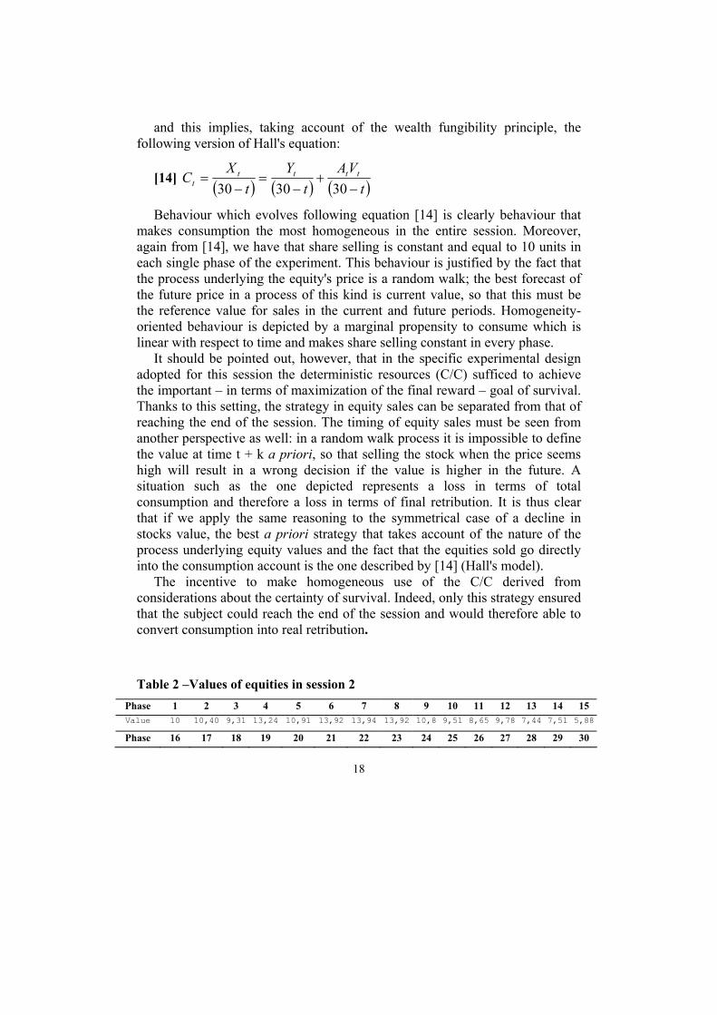
Table 2 –Values of equities in session 2 Phase 1 2 3 4 5 6 7 8 9 10 11 12 13 14 15 Value 10 10,40 9,31 13,24 10,91 13,92 13,94 13,92 10,8 9,51 8,65 9,78 7,44 7,51 5,88
Phase 16 17 18 19 20 21 22 23 24 25 26 27 28 29 30
18

Value 4,26 3,47 4,77 8,51 11,48 15,15 11,37 8,44 8,28 5,28 6,04 3,07 4,61 8,61 5,55
Given the above-reported trend in prices, the theoretical behaviour as
described in equation [14] takes the following form (assuming constant consumption out of deterministic resources):
Figure 1- Possible evolution à la Hall (Benchmark)
0
100
200
300
400
500
600
700
1 2 3 4 5 6 7 8 9 10 11 12 13 14 15 16 17 18 19 20 21 22 23 24 25 26 27 28 29 30Fasi
C/C consumption equities consumption total consumption
Figure 1 shows that in the benchmark model total consumption changes in
direct proportion to the value of equities, and also that this relation is a linear one. Despite variance in the equity wealth, total consumption is rather homogeneous, with limited variability (standard deviation = 33,50).
5.3 SESSION III
As seen, in session 2 the deterministic resources represented by C/C ensured the certainty of survival in that session. For session 3 we decided to increase the minimum consumption level to 600 units of good for each phase. With this change in the experimental design equities assumed an active role in the survival strategy and were no longer to be considered only in "speculative" terms. A posteriori, however, it should be pointed out that the average of the values of equities was greater than 10 Euros and large enough to guarantee survival.
19

In a context like the one depicted above it is not possible to find a single strategy that ensures survival a priori, and neither does Hall’s model give values which are valid beforehand.
One possible strategy for the subjects could have been to"anchor" themselves to the minimal subsistence value of 600 units in each phase. Using a strategy of this kind, total consumption could have consisted mainly of equities when their value was relatively high, and mainly of C/C when their value was relatively low. A possible guess is that the initial value of 10 Euros would be the discriminating factor between the two strategies. This is because the total initial value of equities and C/C was 18000 Euros, which was the sum that enabled the subject to reach the end of the session consuming exactly 600 units in each phase.
Elaborating a strategy in session 3 was a quite complex undertaking, and this suggested that a number of "deaths" would occur during the session. It is of interest to observe how the participants dealt with the change from a situation with a manageable risk of default to one in which survival was strictly linked to the random walk in equity values (see Table 3). Table 3 – Values of equities in session 3
Phase 1 2 3 4 5 6 7 8 9 10 11 12 13 14 15 Value 10 7,81 4,97 1,94 4,32 6,57 6,34 9,93 13,4 10,14 11,64 14,87 11,15 11,36 9,05
Phase 16 17 18 19 20 21 22 23 24 25 26 27 28 29 30 Value 10,98 12,88 12,51 10,75 7,56 8,01 8,18 11,11 14,3 16,24 16,02 18,01 15,89 13,41 13,7
6. DATA ANALYSIS
For a graphic representation of the data collected by means of the experiment see the appendix. There now follows an analysis session by session of the data collected.
6.1 SESSION I
As described above, the main aim of first session was to let subjects learn the general framework of the experiment so that they could more easily tackle subsequent phases. As regards the instructions, retribution in this phase ranged from the minimum amount of 0 Euros to the maximum of 3 Euros. Since the first session was characterized by a static environment, the only explanation for this result isthat the instructions were misunderstood. Only three (15%) of the participants were able to maximize their return, and subject number 8 even used
20

up all her resources before the end. As a general statement, one notes that behaviour was rather random in this session, and it is difficult is to find typical reactions by the experimental subjects. This impression is confirmed by the high average volatility observed in each phase. It should be pointed out, however, that the size of this indicator was increased by the anomalous behaviour of subject 8, who in this sense should be considered an outlier.
6.2 SESSION II
Inspection of the results from session 2, which are summarized in figures 2a and 3a in the appendix, shows that there were four subjects who did not respect constraint (a) and were therefore forced to leave this session with zero retribution. We got this result although the easiness to develop an elementary strategy for surviving in this session. On the other hand, it should be stressed that eleven subjects used all their resources properly, thereby displaying better understanding of the instructions with respect to the previous session. In this sense the subjects proved able to learn from their actions.
On disaggregating the consumption, one notes that there were different underlying approaches to equities and C/C in terms of consumption. Of the subjects who reached the end of the session considered, fourteen sold all their equities and only eleven used their C/C completely.
Average total consumption was very high in the first phases, also because there were two outlier subjects (8 and 14) who used their C/C extensively in these phases. As expected, excessive volatility in consumption led to premature exhaustion of resources. As regards final retribution, it should be noted that, on average and in relative terms, the reward was bigger in this session than in the previous one; and in general that the subjects acted properly with respect to the residual wealth in their portfolios in the last period (complete use was a necessary condition for the maximization of final retribution).
The standard deviation of consumption computed in each phase among the subjects was still rather high, revealing a lack of homogeneous behaviour among the subjects. The standard deviation for each subject across the entire session was also rather high. Of interest is comparison between average standard deviation in consumption (218.9) and the same measure for the benchmark, which was 33.50 and represented the best "smoothing" behaviour given the variability of the stock values. To be noted as regards variance is the behaviour of subject 4, who fixed her consumption in each phase to 500 units and used equities when their value was relatively high, and C/C if they were not. 21

As regards the distribution of equities selling by quantities, Figure 6 in the appendix shows that this was heavily asymmetrical to the left. Small quantity selling, up to 10 units, predominated. The distribution of frequencies considered refers only to the decisions to sell taken by subjects alive in that phase. All values equal to zero are not considered in tables 4 and 5, because associated with this value are both decisions not to sell in that phase and the forced behaviour of the excluded subjects. The frequency distribution of selling decisions was rather dishomogeneous, with a clear predominance of the two lower classes, a central cluster for quantities between 30 and 60, and some isolated action for larger quantities up to 180-190 units (the appendix contains the detailed frequency tables). Table 4 shows that larger quantities of equities were sold when prices of equities were higher. This was an expected observation. Less expected, though, was the amount of selling observed in the first phases and the pronounced reaction in terms of selling after that price rose above the entry price of 10 Euros.
As shown by figure 3a, the selling of equities was sensitive to the trend in values, especially when they were markedly above the entry price of 10 Euros. It should be remembered, however, that the interdependency of the phases made the response of consumption to the values observed biased as time went by.
Analysis of the C/C should bear in mind that in the first phases the presence of "outlying" subjects 8 and 14 added a great deal of noise, and that in the last phase the considerations on maximizing the final retribution altered the behaviour of the subjects. In the other phases, the consumption deriving from C/C was in the neighbourhood of the survival limit of 500. This suggests that a "speculative" approach was taken to equities, which were used as a function of observed, and implicitly forecasted, values. Inspection of individual behaviour shows that three subjects consumed exactly 500 Euros of C/C in each single phase.
6.2.1 COMPARISON WITH THE THEORETICAL BENCHMARK
As stressed when presenting the experiment, session 2 was designed to permit comparison of the behaviour observed with the theoretical benchmark derived from Hall's model (see section 5.2). This comparison is possible either for total consumption or forequity sales. In the theoretical model, the latter are equal to 10, independently of the trend in prices.
A concise representation of the observed average consumption and of that deriving from Hall's model is given by Figure 5, from which it is possible to conclude that up until phase 4 there was excessive average consumption with 22

respect to the benchmark, while from phase 5 to phase 9 the two lines more or less overlapped. From period 10 onwards, the consumption observed was slightly less than the theoretical one and in the neighbourhood of the subsistence level of 500. To be noted is the peak on phase 21, when the value is at its maximum (15,16). The subjects reacted instantaneously to this event, and observing the average value it is understandable that this reaction should be rather homogeneous. Also to be noted is that in the last period the consumption stands above the benchmark and reaches a peak in the last phase. The last movement is indicative of better understanding of the instructions in this phase than in the previous one, but it also reveals that the subjects were unable to allocate resources coherently across the entire session. This difficulty in choosing a broad strategy also emerges from figure 3a, where the trend in values and average equities selling is plotted. In the last phase, subjects sell residuals equities and, unlike in the other phases, the two lines move specularly rather in the same direction.
To be pointed out, too, is that the aggregate observation is influenced by the distorting behaviour of subjects 8 and 14 (see also figure 8), who used all their resources in the first phases, thereby revealing a clear lack of understanding of the instructions. Again referring to the theoretical model, but observing individual behaviour (figure 8), it is evident that the behaviours observed are generally more fragmented than the smooth theoretical one, in particular when peaks in the values are observed. Another relevant observation is that a minority of subjects (3) adopted behaviour similar to that prescribed by Hall's model.
6.3 SESSION III
In session 3 the salient feature emerging from individual data is the high death rate. Indeed, 12 out of 20 subjects did not conclude the session because they had used up all their resources before the end. Among the subjects who developed a successful strategy it is possible to observe a rather strong anchoring to the survival threshold of 600 Euros in total consumption. This kind of cautious behaviour is also observable in the total consumption standard deviation per subject, which is in general lower than in session 2.
Comparison of figure 6 with the trend in equities values shows that on average surviving subjects developed some sort of "rule" on the sale of equities and the use of C/C: when the value is relatively high use equities, and when it is relatively low use C/C. Consumption was generally near to 600 units but in the last phases a large increase in consumption took place.
23

Evident in figures 3b and 4b is the strong reaction in terms of equities sales, and consequently of total consumption, with respect to "high" values. To be stressed is that, although the resources were limited, the two observations, quotations and consumption, moved closely together, especially in the first stages. A more cautious approach would have been more oriented to homogeneity in consumption and to using resources in more balanced manner. With regard to this argument, brief discussion is required of the rule described above. This operational device was biased because it did not take account of the random process governing the trend in values, and it gave rise to consumption which was strongly correlated with the same process. However, as an a posteriori observation, this biased rule proved efficacious in achieving the final goal of survival. Given the uncertain nature of the session, a biased rule helped the subjects to make their choices.
With regard to individual behaviours, attention should be paid to the numerous defaults recorded (12). This large number testifies to the difficulty encountered by many of the participants in developing a "good" strategy. To be noted is the behaviour of subject 18, who set her consumption at the minimum level in each phase but sold equities when their value was low and used C/C when their value was high, thus developing an unsuccessful "counter-rule". The behaviour that adhered most closely to the above rule dwas that of subject 4, who also set consumption to the minimum level but used the two kinds of resources in a "reasonable" manner.
As a general consideration one may say (see also figure 5) that even if the C/C consumption was negatively correlated to the trend in equities, there were small changes in its levels, and throughout the session it remained close to the survival threshold.
Of some interest, too, is the frequency of equities sales (see figure 7 and table 4), which also in this case refers only to positive decisions to sell in the stage considered. As depicted in figure 6, the distribution assumes a more homogeneous shape in this session than in session 2. Most of the observations refer to the 0-5 class, but in this session a closer concentration is observable in the classes from 35 to 60. To be noted is that there are no cases of large entity selling , given that a decision of this kind was not compatible with a coherent strategy in this session. The observation of frequencies seemingly reinforces the guess that survivors followed the simple rule of selling equities when their value was considered high and using C/C when it was not.
24
FINAL REMARKS
From the foregoing analysis of the data we may develop some considerations with regard to the behavioural hypothesis set out in section 2. As regards Prospect Theory, it emerges that for most of the subjects the initial value of 10 Euros was an important reference point for subsequent selling decisions. Many subjects responded to a value below this threshold in central stages with a very small quantity sold. The behaviour described seemed to be widespread, but as an example we may take the average selling in phase 12, when the value rose from 8.66 to 9.79 and the recorded selling value was 2.88. Compare this with the decision in phase 21, when the unit value rose from the 5.16 of the previous phase to 11.37 and the corresponding value was 5.05 (figure 3a). The difference in values is even more striking if we consider the general tendency to sell more in earlier phases. It should be borne in mind, however, that drawing too firm conclusions in terms of prospect theory is dangerous in the experimental setting proposed. The reference point described is less strong than the one observed in reality, where there is a monetary cost of equities, and this may alter the evaluation of losses and gains with respect to the model's indications.
The different approaches to C/C wealth and equities can be better understood by referring to Mental Accounting theory. As stressed above, 14 out of the 16 subjects who successfully completed session 2 sold all the equities at their disposal, and only 11 completely used their C/C. Explanation for this behaviour may be provided by a Mental Accounting approach, but it may also, at least partially, reside in a misunderstanding of the instructions. More evident in terms of Mental Accounting is the behaviour observed in the third session. Observation of the 12 subjects who used up their resources before the end of the session shows that C/C consumption was rather high in all phases, even when the value of equities was high. Default by the participants was due to a lower than expected reaction of C/C consumption to the values of equities. In this respect the selling of equities was much more sensitive to the values observed than was the use of C/C. It is consequently possible to argue that the subjects regarded the C/C as a reserve value on which to define their consumption, and considered equities more as a "speculative" resource. Behaviour of this kind seems to be in line with the hypothesis of non-fungibility of wealth which is the bottom line of the Mental Accounting theory. The Mental Accounting framework is also applicable to subjects who successfully completed the session. The difference between the two groups is that the "winners" were able to allocate resources more appropriately, taking the values of stocks into consideration. From this perspective, maintaining 25

different mental accounts for equities and C/C could foster correct behaviour, because this facilitated the calibration of equities and C/C in an uncertainty governed session like the third one.
In the last session a high death rate was expected, but not so for session 2, when contrary to expectations 4 subjects did not keep enough resources. A possible explanation for this observation may be forthcoming from the concept of Choice Bracketing, and in particular a Narrow Bracketing attitude of the participants. Strong support for this consideration is also provided by the selling of equities recorded in session 2 (figure 3a). Inspection of the average values shows that in the first phases, in particular up until phase 8, sales were rather high. Another interesting point concerning average values is the high level of sales in the last phase. It is possible to deduce from the individual data that behaviour such as that recorded at an aggregate level was due to the interaction between two different profiles of wealth allocation. One group sold a large amount of equities in the first stages, and in so doing the subjects prematurely consumed all their resources. The subjects belonging to the other group sold a few equities during the session and concentrated their sales in the last phase. In both cases it is possible to envisage the existence of a narrow framework to the subjects’ decisions. In the former situation, indeed, the decision-maker failed to consider the total length of the experiment. In the latter, the subjects were too cautious in their selling activity and saw the last phase in isolation, in which they concentrated all their considerations about maximizing the final retribution. Hence the fact that the peak in selling activity is very sharp in the last phase seemingly confirms the hypothesis that the subjects tended to develop a step by step vision of the experiment, rather than a global one. The observed average volatility was rather high, particularly when compared with that of the theoretical model described above, which also represents a Broad Bracketing benchmark. It is possible to state that in general the divergence of an observed behaviour from the model is indicative of a narrow bracketing approach.
As regards the contribution of cognitive dissonance to the experiment’s outcomes, reference must necessarily be made to the above statement about anchoring at the 10 Euro price. With reference to the selling trend observed from phase 18 to phase 21 in session 2 (figure 3a), one notes that four consecutive positive observations are recorded. At the beginning of phase 18 the value is 4.78, at phase 19 it is 8.5, at phase 20 it is 11.49, and finally at phase 21 it is 15.16, which is also the absolute maximum in this session. The average variation in sales between phase 18 and 19 is +0.8 units, and between the subsequent phases it is +9.5 units. Between phases 20 and 21 the recorded variation in selling is +23 units. These figures confirm the hypothesis about 26

behaviour around the "barrier" of 10 Euros. After values cross the entry quotation the owners of stocks exhibit increasing anxiety. This feeling may be determined by rejoicing feelings associated with the belief that one can "forecast" the future trend of prices, maybe by developing a heuristic based on past values. With reference to the possibility of detecting a heuristic in the subjects' behaviour it is interesting to consider phase 21. If the availability heuristic hypothesis were true, we would not observe a single peak in sales, because the previous peak between phase 3 and 7 had a two-peak shape. The scant evidence of heuristics is probably due to the shortness of each session, and consequently to the impossibility of accumulating enough experience. However, although it is not possible to discern specific heuristic-driven behaviour the participants sought to figure out the future evolution of values by themselves. This evidence underlies session 3 and in general plays a major role in the correlation between stock values and selling decisions. The decision to sell substantial amounts when the price is high suggests that the subjects assumed that future prices would be no higher than current ones. A stronger anchoring to the value of 10 is observed, as expected, in session 3 (figure 4b). Important in this regard is comparison of average values between phase 8 and 9. From a methodological standpoint, comparison of adjacent phases has the major advantage of obtaining a more homogeneous distribution of wealth among individuals. At phase 8 the value is 9.93, which is very close to 10, and sales amount to 9.84; at phase 9 the value rises to 13.38 and sales reach the high amount of 14.632.
In general, there may be further confirmations for the hypothesis besides the
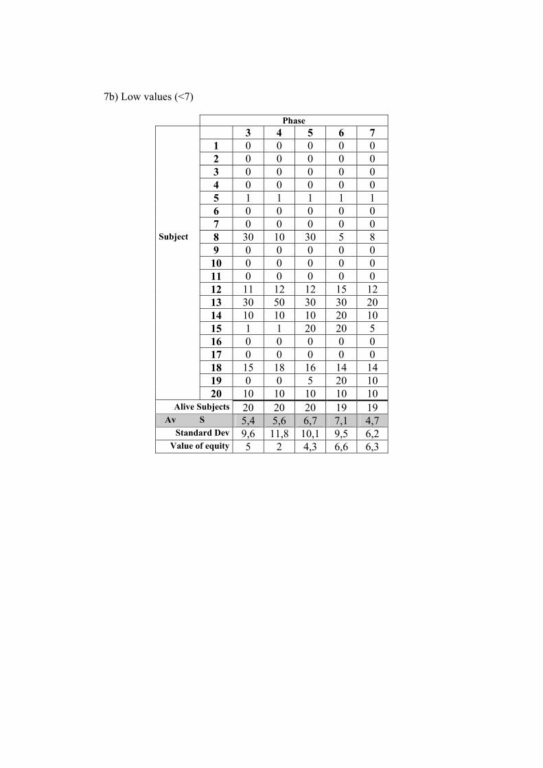
one summarized above. A first important implication of the experiment is that the behaviour observed is in general more complex than that envisaged by standard theories. The subjects tended to ignore the Random Walk nature of equity values and to figure out possible future paths of evolution of the prices for themselves. In session 3, behaviour of this kind seems to facilitate successful conclusion of the session. Further strong evidence is the tendency to consider each phase in isolation, rather than develop a global framework around the sessions. Moreover, C/C wealth and equity wealth are approached differently in terms of opportunity of consumption. When high values are observed, marked peaks in consumption are recorded as well, and the behaviour at phases with high quotations accounts for most of the overall volatility in consumption. As regards the reaction of consumption to low values in price, it should be noted that the experimental setting had a structural limitation in evidencing this decision character due the bottom line represented by the zero value. As also shown in table 6, when the value is below 7 sales are on average 27

around 6 units per phase. The downward change in selling seems proportionally less strong than the upward one. This observation on experimental data resembles the empirical finding with regard to financial markets which highlights the fact that when sharp falls in the stock values are observed, consumption shrinks to a lesser extent than one would expect from the traditional theories. It should be pointed out, however, that the psychological forces underlying experimental choices and real choices may be different in this case. It is likely that experimental observations are driven more by the irrational belief that the value could fall further in the future. Choices in the real world can probably be better explained by concepts like consumption habits and the lack of monetization of nominal losses.
Given that the phenomenon studied in this paper is complex, and given that
the sample used was small, it is important to make clear that the correspondences found between the working hypothesis and the experimental data are mainly an incentive for research to continue in this field using experimental tools. Indeed, it emerges from the research that there is room for analysis of this kind in the intertemporal context. Besides the specific study presented here, there are numerous aspects to be investigated in this field. One such aspect might be the differing impact of losses on consumption when they are effective or when they are only nominal.
Experimental tools coupled with closer attention to the behavioural aspect of decisions in an intertemporal context seem to be a good basis for the development of further research in this field.
28

Figure 2 - Comparison between values of equities (dotted line and left-side vertical axis) and average selling of equities (continuous line and right-side vertical axis).
2a) Session 2
0
5
10
15
20
25
1 3 5 7 9 11 13 15 17 19 21 23 25 27 29
Valu
e
0
10
20
30
40
50
Ave
rage
sel
ling
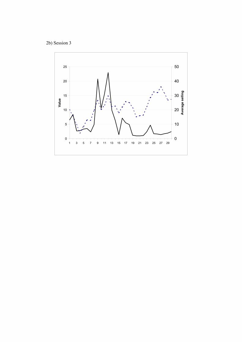
2b) Session 3
0
5
10
15
20
25
1 3 5 7 9 11 13 15 17 19 21 23 25 27 29
Valu
e
0
10
20
30
40
50
Ave
rage
sel
ling

Figure 3 - Comparison between values of equities (dotted line and left-side vertical axis) and average total consumption (continuous line and right-side vertical axis).
3a) Session 2
0
5
10
15
20
25
1 3 5 7 9 11 13 15 17 19 21 23 25 27 29
Valu
e
500
600
700
800
900
1000
Ave
rage
tota
l con
sum
ptio
n

3b) Session 3
0
5
10
15
20
25
1 3 5 7 9 11 13 15 17 19 21 23 25 27 29
Valu
e
600
700
800
900
1000
Ave
rage
tota
l con
sum
ptio
n

Figure 4 - Comparison between average consumption observed in session 2 (continuous line and right-side vertical axis) and theoretical values of the Hall's model (dotted line and left-side vertical axis)
500
600
700
800
900
1000
1 3 5 7 9 11 13 15 17 19 21 23 25 27 29
Hal
l's m
odel
(ben
chm
ark)
500
600
700
800
900
1000
Ave
rage
tota
l con
sum
ptio
n ob
serv
ed
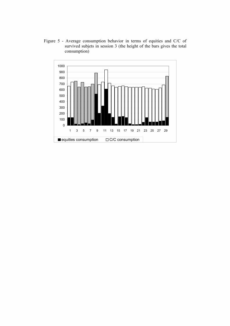
Figure 5 - Average consumption behavior in terms of equities and C/C of survived subjets in session 3 (the height of the bars gives the total consumption)
0
100
200
300
400
500
600
700
800
900
1000
1 3 5 7 9 11 13 15 17 19 21 23 25 27 29
equities consumption
C/C consumption
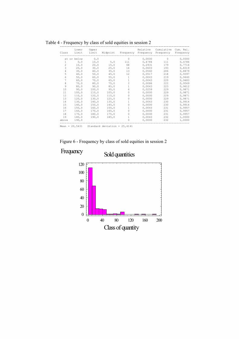
Table 4 - Frequency by class of sold equities in session 2 -------------------------------------------------------------------------------- Lower Upper Relative Cumulative Cum. Rel. Class Limit Limit Midpoint Frequency Frequency Frequency Frequency -------------------------------------------------------------------------------- at or below 0,0 0 0,0000 0 0,0000 1 0,0 10,0 5,0 111 0,4784 111 0,4784 2 10,0 20,0 15,0 68 0,2931 179 0,7716 3 20,0 30,0 25,0 14 0,0603 193 0,8319 4 30,0 40,0 35,0 13 0,0560 206 0,8879 5 40,0 50,0 45,0 12 0,0517 218 0,9397 6 50,0 60,0 55,0 1 0,0043 219 0,9440 7 60,0 70,0 65,0 1 0,0043 220 0,9483 8 70,0 80,0 75,0 2 0,0086 222 0,9569 9 80,0 90,0 85,0 1 0,0043 223 0,9612 10 90,0 100,0 95,0 6 0,0259 229 0,9871 11 100,0 110,0 105,0 0 0,0000 229 0,9871 12 110,0 120,0 115,0 0 0,0000 229 0,9871 13 120,0 130,0 125,0 0 0,0000 229 0,9871 14 130,0 140,0 135,0 1 0,0043 230 0,9914 15 140,0 150,0 145,0 0 0,0000 230 0,9914 16 150,0 160,0 155,0 1 0,0043 231 0,9957 17 160,0 170,0 165,0 0 0,0000 231 0,9957 18 170,0 180,0 175,0 0 0,0000 231 0,9957 19 180,0 190,0 185,0 1 0,0043 232 1,0000 above 190,0 0 0,0000 232 1,0000 -------------------------------------------------------------------------------- Mean = 20,5431 Standard deviation = 25,4141
Figure 6 - Frequency by class of sold equities in session 2
Sold quantities
Class of quantity
Frequency
0 40 80 120 160 2000
20
40
60
80
100
120
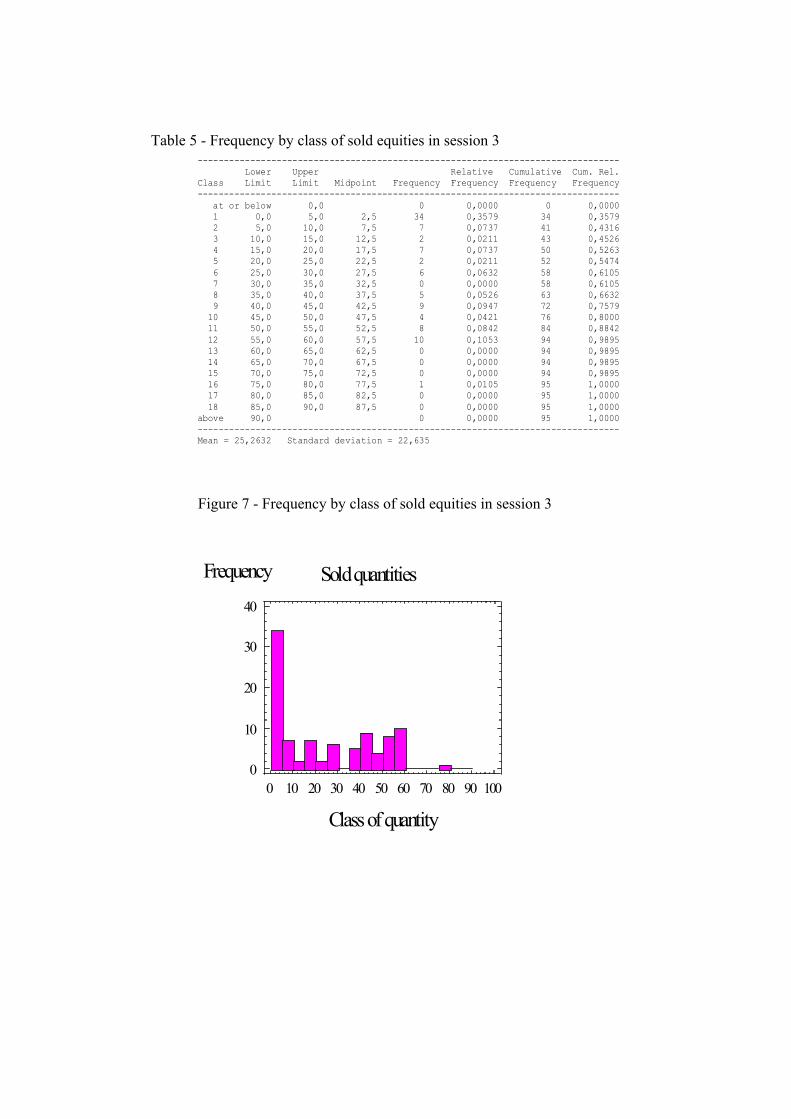
Table 5 - Frequency by class of sold equities in session 3
-------------------------------------------------------------------------------- Lower Upper Relative Cumulative Cum. Rel. Class Limit Limit Midpoint Frequency Frequency Frequency Frequency -------------------------------------------------------------------------------- at or below 0,0 0 0,0000 0 0,0000 1 0,0 5,0 2,5 34 0,3579 34 0,3579 2 5,0 10,0 7,5 7 0,0737 41 0,4316 3 10,0 15,0 12,5 2 0,0211 43 0,4526 4 15,0 20,0 17,5 7 0,0737 50 0,5263 5 20,0 25,0 22,5 2 0,0211 52 0,5474 6 25,0 30,0 27,5 6 0,0632 58 0,6105 7 30,0 35,0 32,5 0 0,0000 58 0,6105 8 35,0 40,0 37,5 5 0,0526 63 0,6632 9 40,0 45,0 42,5 9 0,0947 72 0,7579 10 45,0 50,0 47,5 4 0,0421 76 0,8000 11 50,0 55,0 52,5 8 0,0842 84 0,8842 12 55,0 60,0 57,5 10 0,1053 94 0,9895 13 60,0 65,0 62,5 0 0,0000 94 0,9895 14 65,0 70,0 67,5 0 0,0000 94 0,9895 15 70,0 75,0 72,5 0 0,0000 94 0,9895 16 75,0 80,0 77,5 1 0,0105 95 1,0000 17 80,0 85,0 82,5 0 0,0000 95 1,0000 18 85,0 90,0 87,5 0 0,0000 95 1,0000 above 90,0 0 0,0000 95 1,0000 -------------------------------------------------------------------------------- Mean = 25,2632 Standard deviation = 22,635
Figure 7 - Frequency by class of sold equities in session 3
Sold quantities
Class of q ntity
Frequency
0 10 20 30 40 50 60 70 80 90 100 0
10
20
30
40
ua

values (>13)
Table 6 - Sellings of equities in session 2 divided into "high" and "low" values (<7) of the price of the equities.
6a) High values (>13)
Phase 4 6 7 8 21 1 15 15 15 10 50 2 30 30 0 0 140 3 0 0 0 0 0 4 30 35 35 35 26 5 13 14 13 14 16 6 38 36 37 37 33 7 11 20 20 10 15 8 80 5 5 10 0
9 38 37 25 0 30 10 0 0 0 0 190 11 50 50 50 50 33 12 11 12 14 14 15 13 5 10 10 10 0 14 5 0 0 0 0 15 20 10 10 0 0 16 100 20 10 0 0 17 100 50 20 30 80 18 7 12 12 13 10 19 5 20 20 25 10
Subject
20 14 13 10 10 16 Alive subjects 20 19 19 19 18
Average Sellings 29 20 16 14 37 Standard Dev 31 15 13 15 50
Value of equity 13 14 14 14 15

6b) Low values (<7)
Phase 15 16 17 18 25 26 27 28 30 1 0 0 0 0 0 0 0 0 155 2 0 0 0 0 0 0 0 0 100 3 0 0 0 0 0 0 0 0 0 4 0 0 0 0 0 0 0 0 0 5 5 4 3 4 1 1 1 1 92 6 0 0 0 0 0 0 0 0 0 7 0 0 0 0 0 0 0 0 0
5 5 10
0 0 0 0
0 15 14 0
18 17 17 3,1 1,6 1,9 0,9 ,7 3,6 3 1,7 ,8 5,3 6 3,1
8 0 0 0 0 0 0 0 0 0 9 0 0 0 0 0 0 0 20 40 10 0 0 0 0 0 0 0 0 0 11 0 0 0 0 0 0 0 0 67 12 10 2 15 1 5 10 0 13 20 20 20 0 0 0 0 0 0 14 0 0 0 0 0 0 0 15 0 0 0 0 0 0 0 16 0 0 0 0 0 0 0 0 0 17 0 0 0 0 0 0 0 0 0 18 15 15 17 1 0 0 0 19 2 50 10 20 0 5 10 3
Subject
20 6 6 5 6 6 7 4 10 29 Alive Subjects 18 18 18 16 16 16
Average Sellings 3,2 5,4 3,9 3,2 30 Standard Dev 5,7 12 6,5 5 ,9 5,5 44
Value of equity 5,9 4,3 3,5 4 ,1 4,6 5,6

Table 7 - Sellings of equities in session 3 divided into "high" values (>13) and "low" values (<7) of the price of the equities.
7a) High va Phase
lues (>13)
0 0
5 1 1 1 1 50 40 50 55 80 6 46 41 10 5 0 0 0 0 0 7 100 10 0 0 0 0 0 0 0 0 8 27 0 0 0 05 0 0 0 9 45 40 0 0 0 0 0 0 0 0 1 2 3 0 0 0 0 4 0 0 0 0 0 5 4 0 0 0 6 40 50 0 0 0 0 0 0 0
17 50 100 0 0 0 0 0 0 0 18 7 5 6 4 4 2 6 9 0 19 30 40 20 10 0 0 0 0 0
20 15 18 15 18 1 0 0 0 0
9 12 24 25 26 27 28 29 30 1 60 60 3 0 0 0 0 0 0 2 45 41 43 0 0 0 0 0 0 3 0 0 0 0 0 0 0 0 0 4 44 40 0 0 0 0 0
1 0 60 60 0 0 0 0 0 0 1 45 45 42 16 0 0 0 0 0 1 16 20 15 5 0 0 0 0 0 1 10 10 0 0 0 1 20 10 0 01 30 40 0 0 0 1 1 1
Subject
Alive Subjects 19 18 17 17 17 16 16 16 16 Average Sellings 41,6 45,9 9,3 3,4 3,2 2,68 3,5 4 5
Standard Dev 33,8 38,6 13,3 5,4 11,1 8,9 11,2 12,3 17,9 Value of equity 13,3 14,9 14,3 16,2 16,0 18 15,9 13,4 13,7
7b) Low values (<7)
Phase
4 0 0 0 0 0 5 1 1 1 1 1 6 0 0 0 0 0 7 0 0 0 0 0 8 30 10 30 5 8 9 0 0 0 0 0 10 0 0 0 0 0 11 0 0 0 0 0 1 2 11 12 12 15 1213 30 50 30 30 2014 10 10 10 20 1015 1 1 20 20 5 16 0 0 0 0 0 17 0 0 0 0 0 18 15 18 16 14 1419 0 0 5 20 10
S ect
20 10 10 10 10 10A live Su bjects 20 20 20 19 19e erag el gslin 5,4 5,6 6,7 7,1 4,7 Standar v 10,1 9,5 d De 9,6 11,8 6,2alue quity 5 2 4,3 6,6 6,3
3 4 5 6 7 1 0 0 0 0 0 2 0 0 0 0 0 3 0 0 0 0 0
ubj
Av S
V of e

Comparison between total con
Subject 10
0
500
1000
1500
2000
2500
1 4 7 10 13 16 19 22 25 28
sumption in session 2 (continuous line) and behaviour à la Hall (dotted line)
Subject 1
0
500
1000
1500
2000
2500
1 4 7 10 13 16 19 25 2822
50
100
150
200
250
7 13 1 22
22 2
bjec
0
50
100
150
2000
250
4 7 13 16 22
22 25
ubject 8
150
2000
2500
ubject
0
50
1000
150
200
250
13 16 22 25
Subject 7
0
500
1000
1500
2000
2500
1 4 7 10 13 16 19 22 25 28
Subject 2
0
0
0
0
0
0
1 4 10 6 19 25 28
Subject 3
0
500
1000
1500
2000
2500
1 4 7 10 13 16 19 5 28
Su t 4
0
0
0
0
1 10 19 25 28
Subject 5
0
500
1000
1500
2000
2500
1 4 7 10 13 16 19 28
S
0
500
1000
0
1 4 7 10 13 16 19 22 25 28
Subject 10
0
500
1000
1500
2000
2500
1 4 7 10 13 16 19 22 25 28
S 6
0
0
0
0
1 4 7 10 19 28

0
500
1000
1500
2000
1 4 7 10 13 16 19 22 25 28
0
500
1000
1500
2000
2500
1 4 7 10 13 16 19 22 25 28
Subject 13
0
500
1000
1500
2000
2500
1 4 7 10 13 16 19 22 25 28 Subject 15
0
500
1000
1500
2000
2500
1 4 7 10 13 16 19 22 25 28
Subject 17
0
500
1000
1500
2000
25001 4 7 10 13 16 19 22 25 28
Subject 18
0
500
1000
1500
2000
2500
1 4 7 10 13 16 19 22 25 28
Subject 19
0
500
1000
1500
2000
2500
1 4 7 10 13 16 19 22 25 28
Subject 14
0
500
1000
1500
2000
2500
1 4 7 10 13 16 19 22 25 28
Subject 16
0
500
1000
1500
2000
2500
1 4 7 10 13 16 19 22 25 28
Subject 20
0
500
1000
1500
2000
2500
1 4 7 10 13 16 19 22 25 28
Subject 11 Subject 12 2500

•
•
•
•
•
•
REFERENCES
Anderhub, V. - Guth, W. - Muller, W. - Strobel, M. “An Experimental Analysis of Intertemporal Allocation Behavior” in Experimental Economics, 3(2), 2000
Attanasio, O.P. - Weber, G. “Is Consumption Growth Consistent with Intertemporal Optimization? Evidence from the Consumer Expenditure Survey ” in Journal of Political Economy, 103(6), 1995
Bell, D.E. “Regret in decision making under Uncertainty” in Operations Research, 30(5), 1982
Benartzi, S. - Thaler, R.H. “Myopic Loss Aversion and the Equity Premium Puzzle” in The Quarterly Journal of Economics, 110(1), 1995
Daniel, T.R. “Delay of Consumption and saving Behavior: Some Preliminary, Empirical Outcomes” in “Advances in Economic Psychology” Wiley edito da Antonides, Maital, Van Raaij, 1997
Dynan, K.E. - Maki, D.M. “Does Stock Market Wealth Matter for Consumption?” Federal Reserve Board, Board of Governors http://www.federalreserve.gov/pubs/feds/2001/200123/200123pap.pdf
Festinger, L. –“Teoria della Dissonanza Cognitiva (Introduzione)” VI edizione Franco Angeli Milano, 1996
M.Friedman “A Theory of Consumption” Princeton University Press 1957
Friedman, D. – Sunder, S. “Experimental Economics: A Primer for Economists” Cambridge University Press, 1994
Garcia, R. – Lusardi, A. – Ng, S. “Excess Sensitivity and Asimmetries in consumption: An empirical Investigation” in Journal of Money, Credit and Banking, 29(2), 1997
Gramlich, E.M “Consumption and the wealth effect: The United States and the United Kingdom”, 2002 http://www.federalreserve.gov
Hall, R.H. "Stochastic Implications of the Life Cycle-Permanent Income Hypothesis: Theory and evidence", 1978, JPE
Hey, J. D “Esperimenti in economia” Giappichelli, 1998
•
•
•
•
•
•
•

• Kagel, J.H. - Roth, A. k of Experimental Economics” Princeton University Press, cap.6, 1995
• lec, D. “Anomalies in intertemporal Choice”
• l, Vol 92, 1982
?” sito FED, 1998
ck, NJ:
•
ngs Papers on Economic Activity,
• D. - Loewenstein, G. - Rabin, M. “Choice Bracketing” Journal of Risk and Uncertainty Dicembre, 19(1-3), 1999
• to Sell Winners Too
• vior and the efficiency of Financial System”
• nding” Federal Reserve Board of Governors
E. “The Handboo
• Kahneman, D. - Tversky, A. “Prospect Theory” in “Choices, Values and Frames” Cambridge University Press, 2000
Loewenstein, G. - PreQuarterly Journal of Economics, 1992
Loomes, G. – Sugden, R. “Regret Theory: An Alternative Theory of Rational Choice Under Uncertainty” in Economic Journa
• Ludvingson, S. – Steindel, C. “How Important is The Stock Market Effect on Consumption
• Mankiw, N.G. - Zeldes, S.P. “The consumption of Stockholders and Nonstockholders” in Journal of Financial Economics, 29(1), 1991
• Modigliani, F. & Brumberg, R. (1954): Utility analysis and the consumption function: An interpretation of cross-section data. In: Kurihara, K.K (ed.): Post-Keynesian Economics. New BrunswiRutgers University Press
Palumbo, M.G. - Maki, D.M. “Disentangling The wealth effect: a Cohort Analysis of Household Saving in the ‘90” sito FED, 2001
• Poterba, J. – Samwick, A.A. ”Stock Ownership Patterns, Stock Market Fluctuation and Consumption” Brooki2, 1995
Read,
Shefrin, H. M. - Statman, M. “ The DispositionEarly and Ride Losers Too Long“ 1985 in „Advances in Behavioral Finance“ Russell Sage Foundation New York edito da. Thaler, R.H 1993
Shiller, R.J. “Human behaNBER Working Papers, 1998
Starr McCluer, M. “Stock Market Wealth and Consumer Spe
http://www.federalreserve.gov/pubs/feds/1998/199820/199820pap.pdf
• l Accounts” in Thaler, R.H. “Anomalies: Saving, Fungibility and MentaJournal of Economic Perspectives, 4(1), Winter 1990

• Thaler, R.H. “Mental Accounting Matters” in Journal of Behavioral Decision Making, 1999
• Tversky, A. - Kahneman, D. “Judgement under Uncertainty: Heuristics and Biases” in Science, 1974

Elenco dei papers del Dipartimento di Economia
198 Economic Behaviour: Towards A Constructivist Approach. by Roberto Tamborini. 1989.2 Export Stabilization and Optimal Currency Baskets: the Case of Latin American Countries. by Renzo G.Avesani Giampiero M. Gallo and Peter Pauly. 1989.3 Quali garanzie per i sottoscrittori di titoli di Stato? Una rilettura del rapporto della Commissione Economica dell'Assemblea Costituente di Franco Spinelli e Danilo Vismara. (What Guarantees to the Treasury Bill Holders? The Report of the Assemblea Costituente Economic Commission Reconsidered by Franco Spinelli and Danilo Vismara.) 1989.4 L'intervento pubblico nell'economia della "Venezia Tridentina" durante l'immediato dopoguerra di Angelo Moioli. (The Public Intervention in "Venezia Tridentina" Economy in the First War Aftermath by Angelo Moioli.) 1989.5 L'economia lombarda verso la maturità dell'equilibrio agricolo-commerciale durante l'età delle riforme di Angelo Moioli. (The Lombard Economy Towards the Agriculture-Trade Equilibrium in the Reform Age by Angelo Moioli.) 1989.6 L'identificazione delle allocazioni dei fattori produttivi con il duale. di Quirino Paris e di Luciano Pilati. (Identification of Factor Allocations Through the Dual Approach by Quirino Paris and Luciano Pilati.) 1990.1 Le scelte organizzative e localizzative dell'amministrazione postale: un modello intrpretativo di Gianfranco Cerea. (The Post Service's Organizational and Locational Choices: An Interpretative Model by Gianfranco Cerea.) 1990.2 Towards a Consistent Characterization of the Financial Economy by Roberto Tamborini. 1990.3 Nuova macroeconomia classica ed equilibrio economico generale: considerazioni sulla pretesa matrice walrasiana della N.M.C. di Giuseppe Chirichiello. (New Classical Macroeconomics and General Equilibrium: Some Notes on the Alleged Walrasian Matrix of the N.C.M.by Giuseppe Chirichiello.)
9.1 Knowledge and Prediction of

1990.4 Exch Markets by Roberto Tam
Congestion and Traffic Policy. An Economic Analysis by Giuseppe Folloni and
990.6 Il ruolo della qualità nella domanda di servizi pubblici. Un metodo di analisi
y Luigi Mittone.)
uality: a ote by Pilati Luciano and Giuseppe Ricci.
in an Interdependent World by Luigi Bosco.
consumo, qualità incerta e razionalità limitata di Luigi Mittone e oberto Tamborini.
in the Band: Undeclared Intervention Thresholds in a Target Zone by enzo G. Avesani and Giampiero M. Gallo.
Problem. Capital Flows and the Adjustment of Payments by
992.1 Can People Learn Rational Expectations? An Ecological Approach by Pier Luigi
992.3 Politica tariffaria e politica informativa nell'offerta di servizi pubblici di Luigi
in the Supply of Public Services by Luigi Mittone.)
ange Rate Changes and Price Determination in Polypolistic borini.
1990.5 Congestione urbana e politiche del traffico. Un'analisi economica di Giuseppe Folloni e Gianluigi Gorla. (Urban Gianluigi Gorla.) 1empirica di Luigi Mittone. (The Role of Quality in the Demand for Public Services. A Methodology for Empirical Analysis b 1991.1 Consumer Behaviour under Conditions of Incomplete Information on QN 1991.2 Current Account and Budget Deficit 1991.3 Scelte di R(Consumer Choice, Unknown Quality and Bounded Rationality by Luigi Mittone and Roberto Tamborini.) 1991.4 Jumping R 1991.5 The World Tranfer Roberto Tamborini. 1Sacco. 1992.2 On Cash Dividends as a Social Institution by Luca Beltrametti. 1Mittone (Pricing and Information Policy 1992.4 Technological Change, Technological Systems, Factors of Production by Gilberto Antonelli and Giovanni Pegoretti.

992.5 Note in tema di progresso tecnico di Geremia Gios e Claudio Miglierina.
992.6 Deflation in Input Output Tables by Giuseppe Folloni and Claudio Miglierina.
plessità decisionale: politiche normative e produzione di
sion complexity: normative policies and information production by uigi Mittone)
nd Widening. Responses to Three Institutional Shocks in the
993.1 La tutela dei soggetti "privi di mezzi": Criteri e procedure per la valutazione della
ures for a novel means test by Gianfranco erea )
993.2 La tutela dei soggetti "privi di mezzi": un modello matematico per la
oor: a mathematical model for a novel means test by Wolfgang
993.3 Quasi-markets and Uncertainty: the Case of General Proctice Service by Luigi
993.4 Aggregation of Individual Demand Functions and Convergence to Walrasian
993.5 A Learning Experiment with Classifier System: the Determinants of the Dollar-
993.6 Alcune considerazioni sui paesi a sviluppo recente di Silvio Goglio
Europe: Notes on the Crisis of the EMS by Luigi Bosco)
993.8 Un contributo all'analisi del mutamento strutturale nei modelli input-output di
put-Output Models: a Contribution by Gabriella erloffa)
1(Notes on Technical Progress, by Geremia Gios and Claudio Miglierina). 1 1992.7 Riduzione della cominformazione di Luigi Mittone (Reduction in deciL 1992.8 Single Market Emu aEuropean Community by Pier Carlo Padoan and Marcello Pericoli 1condizione economica di Gianfranco Cerea (Public policies for the poor: criteria and procedC 1rappresentazione della condizione economica di Wolfgang J. Irler (Public policies for the pJ.Irler) 1Mittone 1Equilibria by Dario Paternoster 1Mark Exchange Rate by Luca Beltrametti, Luigi Marengo and Roberto Tamborini 1(Latecomer Countries: Evidence and Comments by Silvio Goglio) 1993.7 Italia ed Europa: note sulla crisi dello SME di Luigi Bosco ( Italy and 1Gabriella Berloffa (Measuring Structural Change in InB

1993.9 On Competing Theories of Economic Growth: a Cross-country Evidence by
aurizio Pugno
993.10 Le obbligazioni comunali di Carlo Buratti (Municipal Bonds by Carlo Buratti)
zazione e il finanziamento della scuola statale di Carlo
he Organization and Financing of Italian State Schools by Carlo Buratti
Hypothesis about regional Growth: Leaders, induced Activities and Policy by
i Mittone.
he punto è la storia d'impresa? Una riflessione storiografica e due ricerche sul ampo a cura di Luigi Trezzi.
futuro dell'impresa cooperativa: tra sistemi, reti ed ibridazioni di Luciano Pilati. the cooperative enterprise: among systems, networks and hybridisation by
995.4 Sulla possibile indeterminatezza di un sistema pensionistico in perfetto equilibrio
tti nd Luigi Bonatti).
an NICs by Maurizio ugno.
atial Diffusion into rugman's Economic Geography by Giuseppe Folloni and Gianluigi Gorla.
conomic Policy Cooperation in a Model with Current Account
M 1 1993.11 Due saggi sull'organizBuratti (Two Essays on t 1994.1 Un'interpretazione della crescita regionale: leaders, attività indotte e conseguenze di policy di Giuseppe Folloni e Silvio Giove. (A Giuseppe Folloni and Silvio Giove). 1994.2 Tax evasion and moral constraints: some experimental evidence by Luigi Bosco and Luig 1995.1 A Kaldorian Model of Economic Growth with Shortage of Labour and Innovations by Maurizio Pugno. 1995.2 A cc 1995.3 Il (The future ofLuciano Pilati). 1finanziario di Luca Beltrametti e Luigi Bonatti. (On the indeterminacy of a perfectly balanced social security system by Luca Beltramea 1995.5 Two Goodwinian Models of Economic Growth for East AsiP 1995.6 Increasing Returns and Externalities: Introducing SpK 1995.7 Benefit of EDynamics and Budget Deficit by Luigi Bosco.

995.8 Coalition and Cooperation in Interdependent Economies by Luigi Bosco.
pubblica italiana e l'ingresso nell'unione monetaria europea di erdinando Targetti.
zi and Paola Villa.
996.2 Keynes' Idea of Uncertainty: a Proposal for its Quantification by Guido Fioretti.
b Trap" in a Dynamic Model of a Dual
996.4 Lebanon: from Development to Civil War by Silvio Goglio.
erspective on the Break-Down of the Relationship between articipation and Fertility by Francesca Bettio and Paola Villa.
sistence in innovative activities? by Elena Cefis.
997.3 A Stability Pact for the EMU? by Roberto Tamborini.
xel Leijonhufvud.
llian Heritage by Axel Leijonhufvud.
997.7 The Multi-Stakeholders Versus the Nonprofit Organisation by Carlo Borzaga and
997.8 How can the Choice of a Tme-Consistent Monetary Policy have Systematic Real
1 1995.9 La finanzaF(Italian Public Finance and the Entry in the EMU by Ferdinando Targetti) 1996.1 Employment, Growth and Income Inequality: some open Questions by Annamaria Simonaz 1 1996.3 The Persistence of a "Low-Skill, Bad-JoLabor Market by Luigi Bonatti. 1 1996.5 A Mediterranean PP 1996.6 Is there any per 1997.1 Imprenditorialità nelle alpi fra età moderna e contemporanea a cura di Luigi Trezzi. 1997.2 Il costo del denaro è uno strumento anti-inflazionistico? di Roberto Tamborini. (Is the Interest Rate an Anti-Inflationary Tool? by Roberto Tamborini). 1 1997.4 Mr Keynes and the Moderns by A 1997.5 The Wickse 1997.6 On pension policies in open economies by Luca Beltrametti and Luigi Bonatti. 1Luigi Mittone. 1Effects? by Luigi Bonatti.

1997.9 Negative Externalities as the Cause of Growth in a Neoclassical Model by Stefano artolini and Luigi Bonatti.
nd Growth in an Evolutionary Game by Angelo Antoci and
ni.
iuseppe Espa.
tive or Optimizing? by Axel Leijonhufvud.
hrough changes y Elisabetta De Antoni.
nd Cross-Sectors omparative Analysis by Elena Cefis and Luigi Orsenigo
998.5 Growth as a Coordination Failure by Stefano Bartolini and Luigi Bonatti
onetary Theory and Central Banking by Axel Leijonhufvud
and growth by aurizio Pugno
998.9 Two types of crisis by Axel Leijonhufvud
998.10 Trade and labour markets: vertical and regional differentiation in Italy by
B 1997.10 Externalities aStefano Bartolini. 1997.11 An Investigation into the New Keynesian Macroeconomics of Imperfect Capital Markets by Roberto Tambori 1998.1 Assessing Accuracy in Transition Probability Matrices by Elena Cefis andG 1998.2 Microfoundations: Adapta 1998.3 Clower’s intellectual voyage: the ‘Ariadne’s thread’ of continuity tb 1998.4 The Persistence of Innovative Activities. A Cross-Countries aC 1 1998.6 M 1998.7 Monetary policy, credit and aggregate supply: the evidence from Italy by RiccardoFiorentini and Roberto Tamborini 1998.8 Stability and multiple equilibria in a model of talent, rent seeking, M 1 1Giuseppe Celi e Maria Luigia Segnana 1998.11 Utilizzo della rete neurale nella costruzione di un trading system by Giulio Pettenuzzo 1998.12 The impact of social security tax on the size of the informal economy by Luigi Bonatti

1999.1 L’economia della montagna interna italiana: un approccio storiografico, a cura di Andrea Leonardi e Andrea Bonoldi.
999.4 The nationalisation of the British Railways in Uruguay, by Giorgio Fodor
r the history of the standard commodity, by Giorgio Fodor
Gaffeo
000.1 A two-sector model of the effects of wage compression on unemployment and
000.2 From Kuwait to Kosovo: What have we learned? Reflections on globalization and
man, by Matteo otterlini
ployment by Maurizio Pugno
Service Sector: an Analysis of the mployment and Welfare Implications, by Luigi Bonatti, Carlo Borzaga and Luigi
001.3 Statistical Economic Approach to Mixed Stock-Flows Dynamic Models in
001.4 The monetary transmission mechanism in Italy: The credit channel and a missing
001.5 Vat evasion: an experimental approach, by Luigi Mittone
1999.2 Unemployment risk, labour force participation and savings, by Gabriella Berloffa e Peter Simmons 1999.3 Economia sommersa, disoccupazione e crescita, by Maurizio Pugno 1 1999.5 Elements fo 1999.6 Financial Market Imperfections, Heterogeneity and growth, by Edoardo 1999.7 Growth, real interest, employment and wage determination, by Luigi Bonatti 2industry distribution of employment, by Luigi Bonatti 2peace, by Roberto Tamborini 2000.3 Metodo e valutazione in economia. Dall’apriorismo a FriedM 2000.4 Under tertiarisation and unem 2001.1 Growth and Monetary Rules in a Model with Competitive Labor Markets, by Luigi Bonatti. 2001.2 Profit Versus Non-Profit Firms in the EMittone. 2Macroeconomics, by Bernardo Maggi and Giuseppe Espa. 2ring, by Riccardo Fiorentini and Roberto Tamborini. 2

2001.6 Decomposability and Modularity of Economic Interactions, by Luigi Marengo, Corrado Pasquali and Marco Valente.
002.1 The Underground Economy and the Underdevelopment Trap, by Maria Rosaria
Perfect apital Mobility and Unionized Labor Markets, by Luigi Bonatti.
002.3 Firms’ bankruptcy and turnover in a macroeconomy, by Marco Bee, Giuseppe
omic tabilization policies in the European Monetary Union, by Roberto Tamborini.
Loans in London 1822-1825, by iorgio Fodor.
itore di Axel Leijonhufvud: le ‘forze oscure del tempo e ell’ignoranza’ e la complessità del coordinamento, by Elisabetta De Antoni.
is Trade between the European Union and the Transition Economies ertical?, by Hubert Gabrisch and Maria Luigia Segnana.
003.1 The service paradox and endogenous economic growth, by Maurizio Pugno.
appe di probabilità di sito archeologico: un passo avanti, di Giuseppe Espa, oberto Benedetti, Anna De Meo e Salvatore Espa.
003.3 The Long Swings in Economic Understianding, by Axel Leijonhufvud.
ia Felice.
tion An Experimental nalysis, by Matteo Ploner.
2001.7 Unbalanced Growth and Women’s Homework, by Maurizio Pugno 2Carillo and Maurizio Pugno. 2002.2 Interregional Income Redistribution and Convergence in a Model with C 2Espa and Roberto Tamborini. 2002.4 One “monetary giant” with many “fiscal dwarfs”: the efficiency of macroecons 2002.5 The Boom that never was? Latin American G 2002.6 L’economia senza bandd 2002.7 WhyV 2 2003.2 MR(Probability maps of archaeological site location: one step beyond, by Giuseppe Espa, Roberto Benedetti, Anna De Meo and Salvatore Espa). 2 2003.4 Dinamica strutturale e occupazione nei servizi, di Giul 2003.5 The Desirable Organizational Structure for Evolutionary Firms in Static Landscapes, by Nicolás Garrido. 2003.6 The Financial Markets and Wealth Effects on ConsumpA


PUBBLICAZIONE REGISTRATA PRESSO IL TRIBUNALE DI TRENTO