wealth and substitution effects in labor and …€¦ · 221 wealth and substitution effects in...
TRANSCRIPT

S O L U T I O N S
8Wealth and Substitution Effects in Laborand Capital Markets
Solutions for Microeconomics: An IntuitiveApproach with Calculus (International Ed.)
Apart from end-of-chapter exercises provided in the student Study Guide, thesesolutions are provided for use by instructors. (End-of-Chapter exercises with
solutions in the student Study Guide are so marked in the textbook.)
The solutions may be shared by an instructor with his or her students at theinstructor’s discretion.
They may not be made publicly available.
If posted on a course web-site, the site must be password protected and foruse only by the students in the course.
Reproduction and/or distribution of the solutions beyond classroom use isstrictly prohibited.
In most colleges, it is a violation of the student honor code for a student toshare solutions to problems with peers that take the same class at a later date.
• Each end-of-chapter exercise begins on a new page. This is to facilitate max-
imum flexibility for instructors who may wish to share answers to some but
not all exercises with their students.
• If you are assigning only the A-parts of exercises in Microeconomics: An In-
tuitive Approach with Calculus, you may wish to instead use the solution set
created for the companion book Microeconomics: An Intuitive Approach.
• Solutions to Within-Chapter Exercises are provided in the student Study Guide.
Wealth and Substitution Effects in Labor and Capital Markets 220
8.1 In this chapter, we began by considering the impact of an increase in the price of gasoline on George
Exxon who owns a lot of gasoline. In this exercise, assume that George and I have exactly the same tastes
and that gasoline and other goods are both normal goods for us.
A: Unlike George Exxon, however, I do not own gasoline but simply survive on an exogenous income
provided to me by my generous wife.
(a) With gallons of gasoline on the horizontal and dollars of other goods on the vertical, graph
the income and substitution effects from an increase in the price of gasoline.
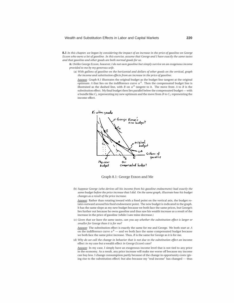
Answer: Graph 8.1 illustrates the original budget as the budget line tangent at the original
optimum A that lies on the indifference curve u A . Then the compensated budget line is
illustrated as the dashed line, with B on u A tangent to it. The move from A to B is the
substitution effect. My final budget then lies parallel below the compensated budget — with
a bundle like C1 representing my new optimum and the move from B to C1 representing the
income effect.
Graph 8.1: George Exxon and Me
(b) Suppose George (who derives all his income from his gasoline endowment) had exactly the
same budget before the price increase that I did. On the same graph, illustrate how his budget
changes as a result of the price increase.
Answer: Rather than rotating inward with a fixed point on the vertical axis, the budget ro-
tates outward around his fixed endowment point. The new budget is indicated in the graph.
It has the same slope as my new budget because we both face the same prices, but George’s
lies further out because he owns gasoline and thus saw his wealth increase as a result of the
increase in the price of gasoline (while I saw mine decrease.)
(c) Given that we have the same tastes, can you say whether the substitution effect is larger or
smaller for George than it is for me?
Answer: The substitution effect is exactly the same for me and George. We both start at A
on the indifference curve u A — and we both face the same compensated budget because
we both face the same price increase. Thus, B is the same for George as it is for me.
(d) Why do we call the change in behavior that is not due to the substitution effect an income
effect in my case but a wealth effect in George Exxon’s case?
Answer: In my case, I simply have an exogenous income level that is not tied to any price
in the economy. As a result, any price increase will make me worse off because my income
can buy less. I change consumption partly because of the change in opportunity costs (giv-
ing rise to the substitution effect) but also because my “real income” has changed — thus

221 Wealth and Substitution Effects in Labor and Capital Markets
the term income effect. The story for George is a bit different — he owns gasoline, and the
value of his wealth from which he can draw income therefore depends on the price of gaso-
line. While an increase in the price of gasoline makes me worse off and decreases my “real
income”, the same increase in price actually makes George better off because it increases
how much income he can draw from what he owns. Put differently, George’s wealth has in-
creased because something he owns has become more valuable — and this will impact his
consumption behavior (in addition to the impact of the change in opportunity costs).
B: In Section 8B.1, we assumed the utility function u(x1,x2) = x0.11
x0.92
for George Exxon as well as
an endowment of gasoline of 1000 gallons. We then calculated substitution and wealth effects when
the price of gasoline goes up from $2 to $4 per gallon.
(a) Now consider me with my exogenous income I = 2000 instead. Using the same utility function
we used for George in the text, derive my optimal consumption of gasoline as a function of p1
(the price of gasoline) and p2 (the price of other goods).
Answer: Solving
maxx1,x2
x0.11 x0.9
2 subject to p1x1 +p2x2 = 2000, (8.1)
we can derive x1 = 200/p1 and x2 = 1800/p2 .
(b) Do I consume the same as George Exxon prior to the price increase? What about after the price
increase?
Answer: Prior to the price increase, p1 = 2 — thus x1 = 200/2 = 100 which is the same as
we calculated in the text for George Exxon. After the price increase, I consume 200/4=50
gallons of gasoline — less than we calculated for George.
(c) Calculate the substitution effect from this price change and compare it to what we calculated
in the text for George Exxon.
Answer: To calculate the substitution effect, we first have to know how much utility I get
before the price increase. We already calculated that x1 = 100, and we can similarly calculate
that x2 = 1800/1 = 1800 (since p2 = 1). My original bundle is therefore A = (100,1800) —
which gives utility u A = u(100,1800) = 1000.118000.9 ≈ 1348 — same as for George Exxon.
Then we ask what the least is that we could spend and reach this utility level again after the
price increase; i.e. we solve
minx1,x2
4x1 +x2 subject to x0.11 x0.9
2 = 1348. (8.2)
Note that this is exactly the same problem we wrote down to determine the substitution
effect for George Exxon in the text — because we are asking exactly the same question. Thus
we get the same answer — x1 = 53.59 and x2 = 1929.19.
(d) Suppose instead that the price of “other goods” fell from $1 to 50 cents while the price of gaso-
line stayed the same at $2. What is the change in my consumption of gasoline due to the
substitution effect? Compare this to the substitution effect you calculated for the gasoline
price increase above.
Answer: We would now solve
minx1 ,x2
2x1 +0.5x2 subject to x0.11 x0.9
2 = 1348. (8.3)
Note that, while this problem looks different from the problem described above in (8.2), it
will necessarily give the same answer because the ratio of the prices is exactly the same, as
is the indifference curve we are trying to fit the compensated budget to. Thus, the solution
will be x1 = 53.59 and x2 = 1929.19 as above — i.e. the substitution effect is the same.
(e) How much gasoline do I end up consuming? Why is this identical to the change in consump-
tion we derived in the text for George when the price of gasoline increases? Explain intuitively
using a graph.
Answer: In B(a) we derived my optimal consumption to be x1 = 200/p1 and x2 = 1800/p2 .
When p1 = 2 and p2 = 0.5, this implies x1 = 100 and x2 = 3600.
Wealth and Substitution Effects in Labor and Capital Markets 222
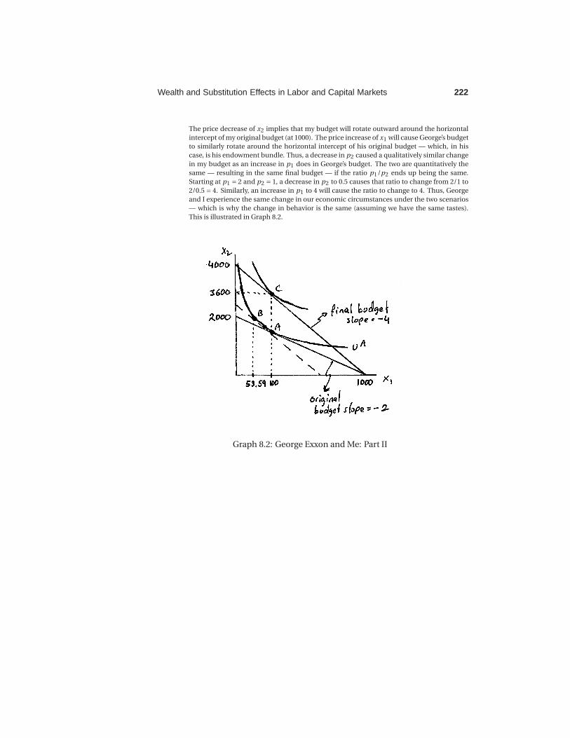
The price decrease of x2 implies that my budget will rotate outward around the horizontal
intercept of my original budget (at 1000). The price increase of x1 will cause George’s budget
to similarly rotate around the horizontal intercept of his original budget — which, in his
case, is his endowment bundle. Thus, a decrease in p2 caused a qualitatively similar change
in my budget as an increase in p1 does in George’s budget. The two are quantitatively the
same — resulting in the same final budget — if the ratio p1/p2 ends up being the same.
Starting at p1 = 2 and p2 = 1, a decrease in p2 to 0.5 causes that ratio to change from 2/1 to
2/0.5 = 4. Similarly, an increase in p1 to 4 will cause the ratio to change to 4. Thus, George
and I experience the same change in our economic circumstances under the two scenarios
— which is why the change in behavior is the same (assuming we have the same tastes).
This is illustrated in Graph 8.2.
Graph 8.2: George Exxon and Me: Part II
223 Wealth and Substitution Effects in Labor and Capital Markets
8.2 As we have suggested in the chapter, it is often important to know whether workers will work more or
less as their wage increases.
A: In each of the following cases, can you tell whether a worker will work more or less as his wage
increases?
(a) The worker’s tastes over consumption and leisure are quasilinear in leisure.
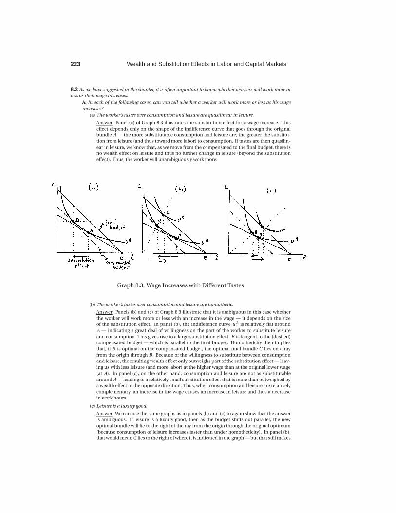
Answer: Panel (a) of Graph 8.3 illustrates the substitution effect for a wage increase. This
effect depends only on the shape of the indifference curve that goes through the original
bundle A — the more substitutable consumption and leisure are, the greater the substitu-
tion from leisure (and thus toward more labor) to consumption. If tastes are then quasilin-
ear in leisure, we know that, as we move from the compensated to the final budget, there is
no wealth effect on leisure and thus no further change in leisure (beyond the substitution
effect). Thus, the worker will unambiguously work more.
Graph 8.3: Wage Increases with Different Tastes
(b) The worker’s tastes over consumption and leisure are homothetic.
Answer: Panels (b) and (c) of Graph 8.3 illustrate that it is ambiguous in this case whether
the worker will work more or less with an increase in the wage — it depends on the size
of the substitution effect. In panel (b), the indifference curve u A is relatively flat around
A — indicating a great deal of willingness on the part of the worker to substitute leisure
and consumption. This gives rise to a large substitution effect. B is tangent to the (dashed)
compensated budget — which is parallel to the final budget. Homotheticity then implies
that, if B is optimal on the compensated budget, the optimal final bundle C lies on a ray
from the origin through B . Because of the willingness to substitute between consumption
and leisure, the resulting wealth effect only outweighs part of the substitution effect — leav-
ing us with less leisure (and more labor) at the higher wage than at the original lower wage
(at A). In panel (c), on the other hand, consumption and leisure are not as substitutable
around A — leading to a relatively small substitution effect that is more than outweighed by
a wealth effect in the opposite direction. Thus, when consumption and leisure are relatively
complementary, an increase in the wage causes an increase in leisure and thus a decrease
in work hours.
(c) Leisure is a luxury good.
Answer: We can use the same graphs as in panels (b) and (c) to again show that the answer
is ambiguous. If leisure is a luxury good, then as the budget shifts out parallel, the new
optimal bundle will lie to the right of the ray from the origin through the original optimum
(because consumption of leisure increases faster than under homotheticity). In panel (b),
that would mean C lies to the right of where it is indicated in the graph — but that still makes
Wealth and Substitution Effects in Labor and Capital Markets 224
it plausible that the wealth effect is smaller than the substitution effect leaving us with less
leisure than at A (and thus more work). In panel (c), C will again lie to the right of where
it is indicated in the graph — but that implies that the wealth effect is even larger and will
still outweigh the substitution effect. This will again leave us with more leisure and thus less
work.
(d) Leisure is a necessity.
Answer: For reasons analogous to those just cited for luxury goods, the answer is still am-
biguous and depends on the size of the substitution effect. This time, C will lie to the left
of where it is marked in panels (b) and (c) of the graph — but that still leaves room for the
ambiguity.
(e) The worker’s tastes over consumption and leisure are quasilinear in consumption.
Answer: Going back to panel (a) of the graph, if consumption is the quasilinear good, then it
will remain unchanged from the optimal bundle B on the compensated budget to the final
budget. This creates a wealth effect on leisure that is opposite to the substitution effect. As
drawn in panel (a), it looks like that returns us to a bundle C that will lie right above A —
thus returning us to the same leisure consumption (and thus the same amount of work) as
before the wage increase. But had we drawn a smaller substitution effect, the horizontal line
through B would take us to the right of A on the final budget — thus causing an increase in
leisure (and a decrease in work). If, on the other hand, we had made the indifference curve
u A flatter and thus had produced a larger substitution effect, the horizontal line through B
would take us to the left of A on the final budget — thus causing a decrease in leisure (and
thus an increase in work) from the original optimum A. As is usually the case when we have
competing substitution and wealth effects, the answer is therefore again ambiguous.
B: Suppose that tastes take the form u(c ,ℓ) = (0.5c−ρ +0.5ℓ−ρ )−1/ρ .
(a) Set up the worker’s optimization problem assuming his leisure endowment is L and his wage
is w.
Answer: The problem is
maxc,ℓ
(0.5c−ρ +0.5ℓ−ρ
)−1/ρsubject to w(L −ℓ) = c. (8.4)
(b) Set up the Lagrange function corresponding to your maximization problem.
Answer: The Lagrange function is
L (c ,ℓ,λ) =(0.5c−ρ +0.5ℓ−ρ
)−1/ρ +λ(wL −wℓ−c). (8.5)
(c) Solve for the optimal amount of leisure.
Answer: The first two first order conditions are
∂L
∂c= 0.5c−(ρ+1) (
0.5c−ρ +0.5ℓ−ρ)−(ρ+1)/ρ −λ= 0,
∂L
∂ℓ= 0.5ℓ−(ρ+1) (
0.5c−ρ +0.5ℓ−ρ)−(ρ+1)/ρ −λw = 0.
(8.6)
The problem simplifies quite a bit if we simply take the λ terms to the other side of each
equation and then divide the second equation by the first — which gives
( c
ℓ
)(ρ+1)= w. (8.7)
If you remember the expression of the MRS for a CES utility function from Chapter 5, you
could have just skipped to this equation — which simply says the MRS is equal to the slope
of the budget. The equation can then be written in terms of just c = ℓw1/(ρ+1). When
plugged into the budget constraint w(L −ℓ) = c , we can solve for
ℓ=L
1+w−ρ/(ρ+1). (8.8)

225 Wealth and Substitution Effects in Labor and Capital Markets
(d) Does leisure consumption increase or decrease as w increases? What does your answer depend
on?
Answer: We can see whether leisure increases or decreases with the wage rate by checking
whether the first derivative of the equation for optimal leisure consumption from above is
positive or negative. This derivative is (after a little algebra)
∂ℓ
∂w= ρ
L(1+w−ρ/(ρ+1)
)−2
(ρ+1)w (2ρ+1)/(ρ+1)
(8.9)
Note L and w are positive and, since ρ lies between −1 and ∞, (ρ+1) is also positive. This
implies that the entire term in the square brackets must be positive regardless of what value
ρ takes. (The negatives in the exponents of course only affect whether the term appears in
the numerator or denominator — not whether it is positive or not.) Since the bracketed term
is positive, the sign of the derivative depends entirely on whether ρ is positive or negative.
If ρ = 0, the tastes are Cobb-Douglas with elasticity of substitution 1/(1−ρ) = 1. In that case,
∂ℓ/∂w = 0 and the wage therefore does not affect leisure consumption (or labor supply).
For ρ < 0 the elasticity of substitution is greater than 1 — and ∂ℓ/∂w < 0. Thus, as the
elasticity of substitution rises above 1, leisure consumption declines with an increase in the
wage — and work hours increase. For ρ > 0, on the other hand, the elasticity of substitution
is less than 1 — and ∂ℓ/∂w > 0. Thus, as the elasticity of substitution falls below 1, leisure
consumption increases with the wage — and work hours fall. (Note that the elasticity of
substitution is σ= 1/(1+ρ).)
(e) Relate this to what you know about substitution and wealth effects in this type of problem.
Answer: We have seen in part A of the question that the substitution effect points to less
leisure (and more work) as wage increases — and, so long as leisure is a normal good, the
wealth effect points in the opposite direction. For homothetic tastes (which CES tastes are),
we showed that the overall effect of a wage increase on leisure consumption then depends
on the substitutability of consumption and leisure. The greater the substitutability, the
larger is the substitution effect — and the larger the substitution effect, the less likely it
is that the wealth effect can fully offset it. We now see that for CES utility functions, the di-
rection of the effect of a wage increase on leisure consumption depends entirely on ρ which
determines the elasticity of substitution or the degree of substitutability between consump-
tion and leisure. Elasticities below 1 make indifference curves look more like those in panel
(c) of Graph 8.3 — with the wealth effect outweighing the substitution effect. Elasticities
above 1, on the other hand, make the indifference curve look more like those in panel (b)
where the substitution effect outweighs the wealth effect.
Wealth and Substitution Effects in Labor and Capital Markets 226
8.3 Suppose that an invention has just resulted in everyone being able to cut their sleep requirement by
10 hours per week — thus providing an increase in their weekly leisure endowment.
A: For each of the cases below, can you tell whether a worker will work more or less?
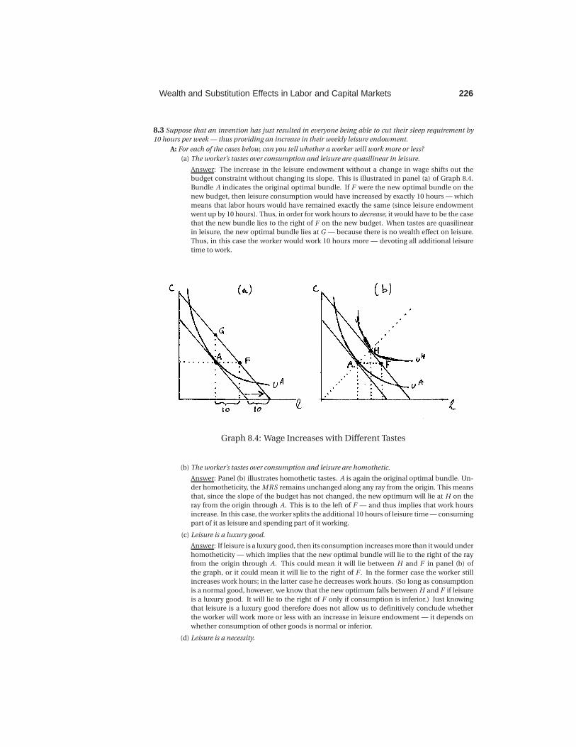
(a) The worker’s tastes over consumption and leisure are quasilinear in leisure.
Answer: The increase in the leisure endowment without a change in wage shifts out the
budget constraint without changing its slope. This is illustrated in panel (a) of Graph 8.4.
Bundle A indicates the original optimal bundle. If F were the new optimal bundle on the
new budget, then leisure consumption would have increased by exactly 10 hours — which
means that labor hours would have remained exactly the same (since leisure endowment
went up by 10 hours). Thus, in order for work hours to decrease, it would have to be the case
that the new bundle lies to the right of F on the new budget. When tastes are quasilinear
in leisure, the new optimal bundle lies at G — because there is no wealth effect on leisure.
Thus, in this case the worker would work 10 hours more — devoting all additional leisure
time to work.
Graph 8.4: Wage Increases with Different Tastes
(b) The worker’s tastes over consumption and leisure are homothetic.
Answer: Panel (b) illustrates homothetic tastes. A is again the original optimal bundle. Un-
der homotheticity, the MRS remains unchanged along any ray from the origin. This means
that, since the slope of the budget has not changed, the new optimum will lie at H on the
ray from the origin through A. This is to the left of F — and thus implies that work hours
increase. In this case, the worker splits the additional 10 hours of leisure time — consuming
part of it as leisure and spending part of it working.
(c) Leisure is a luxury good.
Answer: If leisure is a luxury good, then its consumption increases more than it would under
homotheticity — which implies that the new optimal bundle will lie to the right of the ray
from the origin through A. This could mean it will lie between H and F in panel (b) of
the graph, or it could mean it will lie to the right of F . In the former case the worker still
increases work hours; in the latter case he decreases work hours. (So long as consumption
is a normal good, however, we know that the new optimum falls between H and F if leisure
is a luxury good. It will lie to the right of F only if consumption is inferior.) Just knowing
that leisure is a luxury good therefore does not allow us to definitively conclude whether
the worker will work more or less with an increase in leisure endowment — it depends on
whether consumption of other goods is normal or inferior.
(d) Leisure is a necessity.

227 Wealth and Substitution Effects in Labor and Capital Markets
Answer: If leisure is a necessity, than the new optimum will lie to the left of the ray from the
origin through A. Thus, the new optimum lies to the left of H which means that the worker
will definitely work more hours.
(e) The worker’s tastes over consumption and leisure are quasilinear in consumption.
Answer: Returning to panel (a), quasilinearity in consumption implies that there are no
wealth effects for consumption. Thus, the new optimum will lie at F — which we identified
as the bundle at which work hours remain exactly as they were before (because the worker
simply takes all the additional leisure endowment as leisure consumption).
(f) Do any of your answers have anything to do with how substitutable consumption and leisure
are? Why or why not?
Answer: They do not — because substitution effects arise only when opportunity costs
change — and here no opportunity cost has changed (as seen by the fact that the slope
of the budget constraint does not change.)
B: Suppose that a worker’s tastes for consumption c and leisure ℓ can be represented by the utility
function u(c ,ℓ) = cαℓ(1−α).
(a) Write down the worker’s constrained optimization problem and the Lagrange function used
to solve it, using w to denote the wage and L to denote the leisure endowment.
Answer: The problem is
maxc,ℓ
cαℓ(1−α) subject to w(L −ℓ) = c. (8.10)
The corresponding Lagrange function is
L (c ,ℓ,λ) = cαℓ(1−α) +λ(wL −wℓ−c). (8.11)
(b) Solve the problem to determine leisure consumption as a function of w, α and L. Will an
increase in L result in more or less Leisure consumption?
Answer: The first two first order conditions are
∂L
∂c=αc(α−1)ℓ(1−α) −λ= 0,
∂L
∂ℓ= (1−α)cαℓ−α−λw = 0.
(8.12)
Taking the λ terms to the other side and dividing the equations by one another, we can solve
for c = (α/(1−α))wℓ. Plugging this into the constraint, we can then solve for ℓ = (1−α)L.
Since L clearly enters positively into this equation, an increase in L will increase leisure
consumption. (You can show this more formally by simply taking the derivative of ℓ with
respect to L — which is (1−α) > 0.)
(c) Can you determine whether an increase in leisure will cause the worker to work more?
Answer: Suppose the leisure endowment increases from L to L+H . Then leisure consump-
tion increases from (1−α)L to (1−α)(L+H). The number of hours spent working, however,
is the leisure endowment minus the leisure consumption. Thus, initially the worker works
for L− (1−α)L =αL hours, and after the leisure increase, he works (L+H)− (1−α)(L+H) =α(L+H). Thus, the worker works more after the increase in leisure — and spends a fraction
α of his additional leisure on work.
(d) Repeat the above parts using the utility function u(c ,ℓ) = c +α lnℓ instead.
Answer: The problem now becomes
maxc,ℓ
u(c ,ℓ) = c +α lnℓ subject to w(L −ℓ) = c , (8.13)
with corresponding Lagrange function
L (c ,ℓ,λ) = c +α lnℓ+λ(wL −wℓ−c). (8.14)

Wealth and Substitution Effects in Labor and Capital Markets 228
The first two first order conditions are
∂L
∂c= 1−λ= 0,
∂L
∂ℓ=
α
ℓ−λw = 0.
(8.15)
These solve straightforwardly to ℓ = α/w . Thus, leisure consumption is independent of
leisure endowment (assuming we are not at a corner solution) — which means an increase
in the leisure endowment translates directly into an increase in work hours by the same
amount. This makes sense in light of our answer to A(a) given that the utility function here
treats leisure as a quasilinear good.
(e) Can you show that, if tastes can be represented by the CES utility function u(c ,ℓ) = (αc−ρ(1−α)ℓ−ρ )−1/ρ , the worker will choose to consume more leisure as well as work more when there
is an increase in the leisure endowment L? (Warning: The algebra gets a little messy. You can
occasionally check your answers by substituting ρ = 0 and checking that this matches what
you know to be true for the Cobb-Douglas function u(c ,ℓ) = c0.5ℓ0.5.)
Answer: Setting up the usual maximization problem and solving the first two first order
conditions (or alternatively, recalling the CES formula for MRS and setting it equal to the
slope of the budget line) gives us
c =(
αw
(1−α)
)1/(ρ+1)
ℓ. (8.16)
Substituting this into the constraint w(L −ℓ) = c and solving for ℓ we get
ℓ=L
1+ (αw−ρ/(1−α))1/(ρ+1). (8.17)
(You can check that this is correct by substituting ρ = 0 to see if it gives the Cobb-Douglas
answer ℓ = (1−α)L — which it does.) The derivative of this function with respect to L is
positive (since all the terms in the denominator are positive given 0 < α < 1 and w > 0.
Thus, leisure consumption increases with leisure endowment regardless of the value of ρ —
and thus regardless of the elasticity of substitution.
Labor hours l are just given by L minus leisure consumption; i.e.
l = L −L
1+ (αw−ρ/(1−α))1/(ρ+1)=
L(αw−ρ/(1−α)
)1/(ρ+1)
1+ (αw−ρ/(1−α))1/(ρ+1). (8.18)
(You can again check that this is correct by substituting ρ = 0 to see if it gives the Cobb-
Douglas answer l =αL — which it does.) The derivative of this with respect to L is similarly
positive regardless of ρ. Thus, regardless of the elasticity of substitution, work hours in-
crease as leisure endowment rises.
229 Wealth and Substitution Effects in Labor and Capital Markets
8.4 Business Application: Merchandise Exchange Policies: Suppose you have $200 in discretionary in-
come that you would like to spend on ABBA CDs and Arnold Schwarzenegger DVDs.
A: On the way to work, you take your $200 to the Wal-Mart and buy 10 CDs and 5 DVDs at CD prices
of $10 and DVD prices of $20.
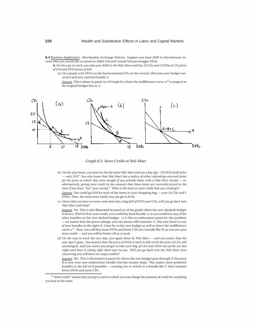
(a) On a graph with DVDs on the horizontal and CDs on the vertical, illustrate your budget con-
straint and your optimal bundle A.
Answer: This is done in panel (a) of Graph 8.5 where the indifference curve u A is tangent to
the original budget line at A.
Graph 8.5: Store Credit at Wal-Mart
(b) On the way home, you drive by the the same Wal-Mart and see a big sign: “All DVDs half-price
— only $10!” You also know that Wal-Mart has a policy of either refunding returned items
for the price at which they were bought if you provide them with a Wal-Mart receipt — or,
alternatively, giving store credit in the amount that those items are currently priced in the
store if you have “lost” your receipt.1 What is the most in store credit that you could get?
Answer: You could get $10 for each of the items in your shopping bag — your 10 CDs and 5
DVDs. Thus, the most store credit you can get is $150.
(c) Given that you have no more cash and only a bag full of DVDs and CDs, will you go back into
Wal-Mart and shop?
Answer: Yes. This is also illustrated in panel (a) of the graph where the new (dashed) budget
is drawn. With $150 in store credit, you could buy back bundle A, or you could buy any of the
other bundles on the new dashed budget. (A is like an endowment point for this problem
— no matter how the prices change, you can always still consume A.) But now there is a set
of new bundles to the right of A that lie on the new budget as well as above the indifference
curve u A . Thus, you will buy more DVDs and fewer CDs (at a bundle like B ) as you use your
store credit — and you will be better off as a result.
(d) On the way to work the next day, you again drive by Wal-Mart — and you notice that the
sale sign is gone. You assume that the price of DVDs is back to $20 (with the price of CDs still
unchanged), and you notice you forgot to take your bag of CDs and DVDs out of the car last
night and have it sitting right there next to you. Will you go back into the Wal-Mart store
(assuming you still have an empty wallet)?
Answer: Yes. This is illustrated in panel (b) where the new budget goes through B (because
B is now your new endowment bundle) but has steeper slope. This makes more preferred
bundles to the left of B possible — causing you to switch to a bundle like C that contains
fewer DVDs and more CDs.
1“Store credit” means that you get a card to which you can charge the amount of credit for anything
you buy in the store.
Wealth and Substitution Effects in Labor and Capital Markets 230
(e) Finally, you pass Wal-Mart again on the way home — and this time see a sign: “Big Sale — All
CDs only $5, All DVDs only $10!” With your bag of merchandise still sitting next to you and
your wallet still empty, will you go back into Wal-Mart?
Answer: No, you will not. The slope of the last budget constraint you faced at Wal-Mart was
−2 — and resulted in you leaving with bundle C in panel (b) of the graph. C is now your
new endowment bundle. When prices of both CDs and DVDs fall by the same proportion,
the ratio of the price of DVDs to CDs is still 2 (i.e. 10/5=2) — which implies the slope of the
budget is not changing. If you went back into Wal-Mart, you could therefore get store credit
in an amount that would allow you to buy C again — or any bundle on the budget that goes
through C with slope −2. But that is the same budget you had in the morning — which
would mean C , the bundle that is in your bag already, would still be the optimal bundle.
(f) If you are the manager of a Wal-Mart with this “store credit” policy, would you tend to favor
— all else being equal — across the board price changes or sales on selective items?
Answer: All else being equal, you would favor across the board price cuts. These would keep
the ratio of prices the same and would make it impossible for people to game the store credit
policy. Selective price changes, as we have seen — whether they are increases or decreases
— make it possible for people to game the system.
(g) True or False: If it were not for substitution effects, stores would not have to worry about
people gaming their “store credit” policies as you did in this example.
Answer: This is true. To see this, we can draw an indifference curve without any substi-
tutability at the original optimal bundle A. This is done in panel (c) of Graph 8.5. The steeper
slope is the original budget. When the price of DVDs falls, the new budget goes through A
but has half the slope. Without any substitutability between the goods, this would imply
that A is still the optimal bundle — i.e. A=B . Then the price of DVDs increases again —
causing the budget constraint to revert back to the original. A is still optimal — i.e. A=C .
B: Suppose your tastes for DVDs (x1) and CDs (x2) can be characterized by the utility function
u(x1,x2) = x0.51 x0.5
2 . Throughout, assume that it is possible to buy fractions of CDs and DVDs.
(a) Calculate the bundle you initially buy on your first trip to Wal-Mart.
Answer: By now you probably probably realize that, when tastes are Cobb-Douglas and
the exponents sum to 1, the optimal quantity of each good is the exponent on that good
times income divided by the good’s price. (You can of course derive this by solving the usual
maximization problem.) This gives us
x1 =0.5I
p1=
0.5(200)
20= 5 and x2 =
0.5I
p2=
0.5(200)
10= 10. (8.19)
Your original bundle A is therefore (5,10) (as in part A of the question).
(b) Calculate the bundle you buy on your way home from work on the first day (when p1 falls to
10).
Answer: The value of your goods when exchanged for store credit when p1 = p2 = 10 is
$150. When dealing with endowments, this value of the endowment takes the place of the
exogenous income I in our equations. Thus, using the same insight about the equations for
optimal consumption under Cobb-Douglas tastes as we used in B(a), we get
x1 =0.5(150)
10= 7.5 and x2 =
0.5(150)
10= 7.5. (8.20)
In essence, you are trading 2.5 CDs for 2.5 DVDs because the opportunity cost of DVD’s has
fallen.
(c) If you had to pay the store some fixed fee for letting you get store credit, what’s the most you
would be willing to pay on that trip?
Answer: The most you’d be willing to pay is an amount that will make you as well off after
using your store credit as you were before you went back into Wal-Mart. Before you went
back in, you had 5 DVDs and 10 CDs — which gave you utility u A = 50.5100.5 ≈ 7.071. To
calculate the bundle on that same indifference curve that you would buy if you paid the
maximum bribe fee you are willing to pay, we have to solve the problem

231 Wealth and Substitution Effects in Labor and Capital Markets
minx1,x2
10x1 +10x2 subject to x0.51 x0.5
2 = 7.071. (8.21)
Setting up the Lagrange function and solving the first two first order conditions, we get x1 =x2. Plugging this back into the constraint and solving, we get x1 = 7.071 = x2. This bundle
costs 10(7.071)+10(7.071) ≈ 141.42. Thus, you would be willing to pay up to about $8.58 to
be able to get store credit at Wal-Mart.
(d) What bundle will you eventually end up with if you follow all the steps in part A?
Answer: Eventually you go back and exchange your x1 = x2 = 7.071 bundle for store credit
when p1 = 20 and p2 = 10. This would give you store credit of 20(7.071) + 10(7.071) ≈$212.13. With that, you would buy
x1 =0.5(212.13)
20≈ 5.30 and x2 =
0.5(212.13)
10≈ 10.61. (8.22)
(e) Suppose that your tastes were instead characterized by the function u(x1,x2) = (0.5x−ρ1
+0.5x
−ρ2 )−1/ρ . Can you show that your ability to game the store credit policy diminishes as the
elasticity of substitution goes to zero (i.e. as ρ goes to ∞)?
Answer: If we solve
maxx1,x2
(0.5x
−ρ1
+0.5x−ρ2
)−1/ρsubject to p1 x1 +p2 x2 = I (8.23)
in the usual way, we get
x1 =I
p1 +p1/(ρ+1)1 p
ρ/(ρ+1)2
and x2 =I
p2 +p1/(ρ+1)2 p
ρ/(ρ+1)1
. (8.24)
Note that the limit of 1/(ρ+1) as ρ goes to ∞ is 0, and the limit of ρ/(ρ+1) as ρ goes to ∞ is
1. Thus, the limit of the solutions for x1 and x2 as ρ goes to ∞ is
x1 =I
p1 +p01 p1
2
=I
p1 +p2and x2 =
I
p2 +p11 p0
2
=I
p1 +p2. (8.25)
Initially, I = 200, p1 = 20 and p2 = 10. Thus, x1 = 200/(20 + 10) = 6.67 = x2. Thus, the
initial optimum is A=(6.67,6.67). Then p1 falls to 10. The value of the endowment A is the
10(6.67)+10(6.67) = 133.33. Plugging this into our equations for x1 and x2 — and using the
new prices p1 = p2 = 10 — we get x1 = 133.33/(10+10) = 6.67 = x2. Thus, our new optimal
bundle if we use store credit is B =(6.67,6.67) which is equal to A. Nothing was gained by
using the store credit. When p1 then goes back to 20, store credit for this bundle is back to
$200 — which implies the optimal bundle is once again A.
Wealth and Substitution Effects in Labor and Capital Markets 232
8.5 Policy Application: Savings Behavior and Tax Policy: Suppose you consider the savings decisions of
three households - households 1, 2 and 3. Each household plans for this year’s consumption and next
year’s consumption, and each household anticipates earning $100,000 this year and nothing next year.
The real interest rate is 10%. Assume throughout that consumption is always a normal good.
A: Suppose the government does not impose any tax on interest income below $5,000 but taxes any
interest income above $5,000 at 50%.
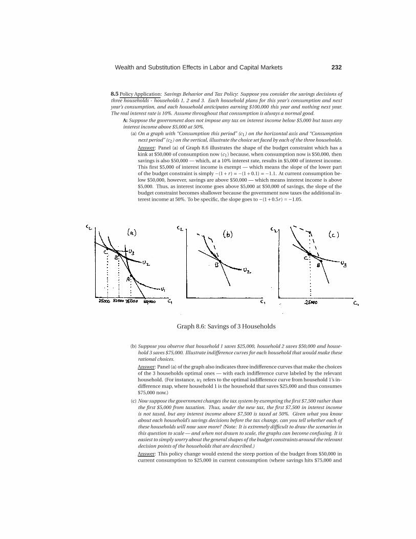
(a) On a graph with “Consumption this period” (c1) on the horizontal axis and “Consumption
next period” (c2) on the vertical, illustrate the choice set faced by each of the three households.
Answer: Panel (a) of Graph 8.6 illustrates the shape of the budget constraint which has a
kink at $50,000 of consumption now (c1) because, when consumption now is $50,000, then
savings is also $50,000 — which, at a 10% interest rate, results in $5,000 of interest income.
This first $5,000 of interest income is exempt — which means the slope of the lower part
of the budget constraint is simply −(1+ r ) =−(1+0.1) =−1.1. At current consumption be-
low $50,000, however, savings are above $50,000 — which means interest income is above
$5,000. Thus, as interest income goes above $5,000 at $50,000 of savings, the slope of the
budget constraint becomes shallower because the government now taxes the additional in-
terest income at 50%. To be specific, the slope goes to −(1+0.5r ) =−1.05.
Graph 8.6: Savings of 3 Households
(b) Suppose you observe that household 1 saves $25,000, household 2 saves $50,000 and house-
hold 3 saves $75,000. Illustrate indifference curves for each household that would make these
rational choices.
Answer: Panel (a) of the graph also indicates three indifference curves that make the choices
of the 3 households optimal ones — with each indifference curve labeled by the relevant
household. (For instance, u1 refers to the optimal indifference curve from household 1’s in-
difference map, where household 1 is the household that saves $25,000 and thus consumes
$75,000 now.)
(c) Now suppose the government changes the tax system by exempting the first $7,500 rather than
the first $5,000 from taxation. Thus, under the new tax, the first $7,500 in interest income
is not taxed, but any interest income above $7,500 is taxed at 50%. Given what you know
about each household’s savings decisions before the tax change, can you tell whether each of
these households will now save more? (Note: It is extremely difficult to draw the scenarios in
this question to scale — and when not drawn to scale, the graphs can become confusing. It is
easiest to simply worry about the general shapes of the budget constraints around the relevant
decision points of the households that are described.)
Answer: This policy change would extend the steep portion of the budget from $50,000 in
current consumption to $25,000 in current consumption (where savings hits $75,000 and
233 Wealth and Substitution Effects in Labor and Capital Markets
thus interest income hits $7,500). Household 1 would be unaffected by this change since the
indifference curve u1 that is tangent at A lies above any new bundle that becomes available
as a result of the policy change. Thus, household 1’s savings would not change.
Household 2’s savings, on the other hand, would almost certainly increase. In order for B to
be optimal before the policy change, this household has an indifference curve that “hangs”
on the kink of the original budget constraint. That means the MRS could lie between −1.1
(which is the slope of the steep portion of the budget) and −1.05 (which is the slope of the
shallower portion). If the MRS =−1.1 at B , then the indifference curve u2 is tangent to the
extended steep budget that runs through B after the policy change — and thus B would
continue to be optimal. However, if the MRS falls anywhere from −1.05 to −1.1 at B , then
the new (dashed) budget constraint will cut the indifference curve u2 as illustrated in panel
(b) of Graph 8.6 — thus enabling the household to choose from a set of new bundles that lie
above the original indifference curve. All of these bundles are such that consumption now
(c1) falls — i.e. savings increases.
Household 3, however, will definitely not save more. Panel (c) of the graph illustrates the
change for this household. The new kink point now happens right above C . If the household
were to choose a bundle on the flat portion of the new (dashed) budget line, then c1 would
be an inferior good and we have assumed that consumption is always normal. (It would
be inferior because, when faced with a parallel outward shift in the budget, the household
would be choosing to consume less.) Thus we know that the household will choose either
the kink point (and keep savings the same) or a point on the steeper portion of the new
(dashed) budget — with more c1 and thus less savings.
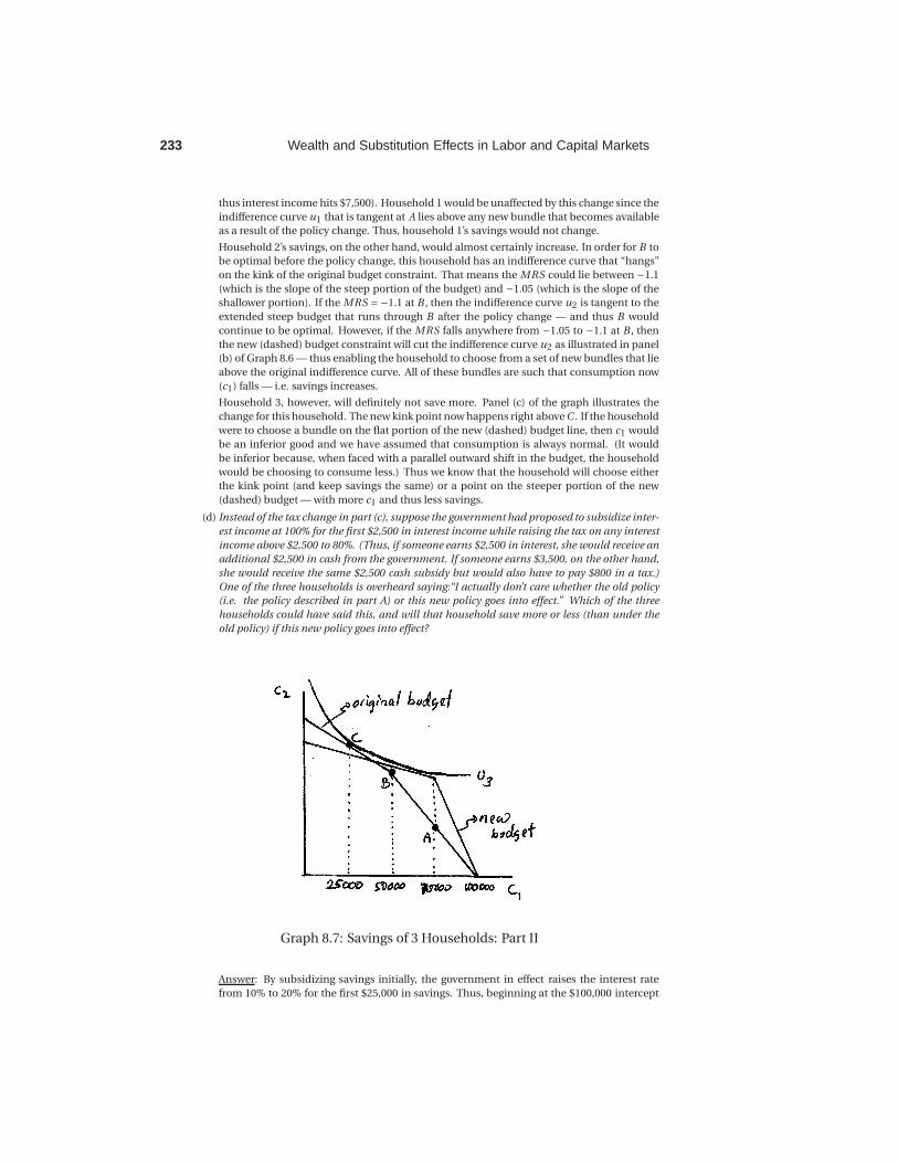
(d) Instead of the tax change in part (c), suppose the government had proposed to subsidize inter-
est income at 100% for the first $2,500 in interest income while raising the tax on any interest
income above $2,500 to 80%. (Thus, if someone earns $2,500 in interest, she would receive an
additional $2,500 in cash from the government. If someone earns $3,500, on the other hand,
she would receive the same $2,500 cash subsidy but would also have to pay $800 in a tax.)
One of the three households is overheard saying:“I actually don’t care whether the old policy
(i.e. the policy described in part A) or this new policy goes into effect.” Which of the three
households could have said this, and will that household save more or less (than under the
old policy) if this new policy goes into effect?
Graph 8.7: Savings of 3 Households: Part II
Answer: By subsidizing savings initially, the government in effect raises the interest rate
from 10% to 20% for the first $25,000 in savings. Thus, beginning at the $100,000 intercept
Wealth and Substitution Effects in Labor and Capital Markets 234
on the c1 axis, the budget constraint is twice as steep. From that point on, however, the
government is in effect reducing the interest rate from 10% to 2% because of the 80% tax
on interest income. Thus, beginning at $75,000 of current (c1) consumption and moving
leftward, the budget constraint becomes shallower than it was before. It seems clear that
the two budget constraints will cross at some point — the question is where. We can check,
for instance, which budget gives higher consumption next period (c2) at $50,000 of savings
where the original kink occurred. Under the original policy, you make $5,000 in interest
when you save $50,000 — giving you c2 = $55,000. Under the new policy, you get $5,000
of interest (including the subsidy) for the first $25,000 you save, you earn another $2,500
of interest for the next $25,000 in savings — but that is taxed at 80% to leave you with only
$500 of after-tax interest income. Thus, your total interest income (including the subsidy
and subtracting out the tax) is $5,500 — leaving you with $55,500 in c2. This is $500 more
than under the original policy. If you save an additional $25,000 (for a total of $75,000), you
would earn an additional $2,500 in interest. Under the original policy, half of that would be
taxed away, leaving you with $1,250. Under the new policy, 80% is taxed away — leaving you
with only $500 more. Thus, at $75,000 of savings, the old policy results in greater c2 than
the new policy — $250 more, to be exact. The old and the new budgets therefore intersect
between $75,000 and $50,000 in savings.
The general relationship between the original and the new budget constraints is graphed in
Graph 8.7 (previous page). Households 1 and 2 must prefer the new policy since it opens
up new bundles to the northeast of their original optimal bundles. Household 3, however,
might be indifferent — as illustrated with the indifference curve u3. Under the new policy,
household 3 would then consume more now — and save less — if indeed it is indifferent
between the policies.
B: Now suppose that our 3 households had tastes that can be represented by the utility function
u(c1,c2) = cα1 c(1−α)2 , where c1 is consumption now and c2 is consumption a year from now.
(a) Suppose there were no tax on savings income. Write down the intertemporal budget con-
straint with the real interest rate denoted r and current income denoted I (and assume that
consumer anticipate no income next period).
Answer: The intertemporal budget constraint is
(1+ r )c1 +c2 = (1+ r )I . (8.26)
(b) Write down the constrained optimization problem and the accompanying Lagrange function.
Then solve for c1, current consumption, as a function of α, and solve for the implied level of
savings as a function of α, I and r . Does savings depend on the interest rate?
Answer: The maximization problem is
maxc1 ,c2
cα1 c(1−α)2 subject to (1+ r )c1 +c2 = (1+ r )I . (8.27)
The Lagrange function for this problem is
L (c1,c2,λ) = cα1 c(1−α)2
+λ((1+ r )I − (1+ r )c1 −c2). (8.28)
The first two first order conditions can be solved to yield
c2 =(1−α)(1+ r )
αc1. (8.29)
Plugging this into the constraint (1+ r )c1 +c2 = (1+ r )I , we can solve for c1 =αI . Savings s
is then simply c1 subtracted from current income; i.e.
s = I −αI = (1−α)I . (8.30)
Savings therefore does not depend on the interest rate.
(c) Determine the α value for consumer 1 as described in part A.
Answer: Consumer 1 saves 25% of her income on the portion of the budget where there is
no tax — thus, it must be that (1−α) = 0.25 or α= 0.75.

235 Wealth and Substitution Effects in Labor and Capital Markets
(d) Now suppose the initial 50% tax described in part A is introduced. Write down the budget
constraint (assuming current income I and before-tax interest rate r ) that is now relevant for
consumers who end up saving more than $50,000. (Note: Don’t write down the equation for
the kinked budget — write down the equation for the linear budget on which such a consumer
would optimize.)
Answer: To write down this budget, we need to know an intercept and a slope. The slope
is simply −(1+0.5r ) since the government is taxing interest income at 50%. We can deter-
mine the c2 intercept by calculating the total interest a consumer would earn if she saved
all her income I assuming I > 50,000. For the first $50,000, she would save at the un-
taxed interest rate of r — thus accumulating (1+ r )50000 for next period. She would then
have (I − 50000) left to save — on which she would earn 0.5r interest. In addition to ac-
cumulating (1 + r )50000 for the first $50,000 in savings, she would therefore accumulate
(1+0.5r )(I −50000) if she saved all her income. Her total possible c2 consumption is there-
fore
(1+ r )50000+ (1+0.5r )(I −50000) = (1+0.5r )I +25000r. (8.31)
This, then, is the c2 intercept. Given we already determined the slope to be −(1+0.5r ), the
budget constraint is c2 = (1+0.5r )I +25000r − (1+0.5)c1 or
(1+0.5r )c1 +c2 = (1+0.5r )I +25000r. (8.32)
(e) Use this budget constraint to write down the constrained optimization problem that can be
solved for the optimal choice given that households save more than $50,000. Solve for c1 and
for the implied level of savings as a function of α, I and r .
Answer: The maximization problem is
maxc1,c2
cα1 c(1−α)2 subject to (1+0.5r )c1 +c2 = (1+0.5r )I +25000r. (8.33)
The Lagrange function for this problem is
L (c1,c2,λ) = cα1 c(1−α)2 +λ((1+0.5r )I +25000r − (1+0.5r )c1 −c2). (8.34)
Solving this in the same way as before, we then get
c1 =αI +25000αr
(1+0.5r )(8.35)
and an implied savings s of
s = (1−α)I −25000αr
(1+0.5r ). (8.36)
(f) What value must α take for household 3 as described in part A?
Answer: Household 3 saves $75,000 with income of $100,000 and before-tax interest rate
r = 0.1. Thus
75000 = (1−α)100000−25000α(0.1)
(1+0.5(0.1))(8.37)
which solves to α≈ 0.244.
(g) With the values of α that you have determined for households 1 and 3, determine the impact
that the tax reform described in (c) of part A would have?
Answer: Using panels (b) and (c) of Graph 8.6, we concluded in part A that both households
will choose to locate on the steeper portion of the budget under the new policy — i.e. on
the portion defined by the constraint (1+ r )c1 +c2 = (1+ r )I where I = 100,000 and r = 0.1.
In B(b), we determined that savings in this case is given by s = (1−α)I . Thus, household 1
for whom α= 0.75 would save (1−0.25)100,000 = 25,000 as before. Household 3, for whom
α≈ 0.244, will save approximately (1−0.244)100,000 = 75,600 — but that level of savings lies
to the left of the kink point of the dashed budget in panel (c). Thus, household 3 optimizes
at the kink point, implying unchanged savings at $75,000.

Wealth and Substitution Effects in Labor and Capital Markets 236
(h) What range of values can α take for household 2 as described in part A?
Answer: There are several ways you could use to figure this out. One way is to note that
MRS =−αc2
(1−α)c1(8.38)
and that this must, for household 2, lie between −1.05 and −1.10 at (c1,c2)= (50000,55000)
in order for that kink point in the budget to be optimal. Substituting these values for c1 and
c2 into the expression for MRS and setting it equal to these two endpoint values, we can
solve
−55000α
50000(1−α)=−1.05 and −
55000α
50000(1−α)=−1.10 (8.39)
to conclude that 0.488 ≤α≤ 0.5.
Another way to solve for this is to use our results from the previous parts. Household 2
might have a tangency with the steep portion of the budget at (c1,c2) = (50000,55000). We
concluded in B(b) (equation (8.30)) that in this case, savings s is s = (1 −α)I . Thus, for
household 2 to choose $50,000 in savings under the steeper portion of the budget, 50000 =(1−α)100000 which implies α= 0.5.
Alternatively, household 2 could have a tangency with the shallow portion of the budget at
(c1,c2) = (50000,55000). We concluded in B(3) that savings then satisfies equation (8.36).
Substituting s = 50,000, I = 100,000 and r = 0.1 into that equation, we can solve for α ≈0.488. Thus, again we get that 0.488 ≤α≤ 0.5.
237 Wealth and Substitution Effects in Labor and Capital Markets
8.6 Policy Application: The Earned Income Tax Credit: Since the early 1970’s, the U.S. government has
had a program called the Earned Income Tax Credit (previously mentioned in end-of-chapter exercises in
Chapter 3.) A simplified version of this program works as follows: The government subsidizes your wages
by paying you 50% in addition to what your employer paid you but the subsidy applies only to the first
$300 (per week) you receive from your employer. If you earn more than $300 per week, the government
gives you only the subsidy for the first $300 you earned but nothing for anything additional you earn. For
instance, if you earn $500 per week, the government would give you 50% of the first $300 you earned — or
$150.
A: Suppose you consider workers 1 and 2. Both can work up to 60 hours per week at a wage of $10
per hour, and after the policy is put in place you observe that worker 1 works 39 hours per week while
worker 2 works 24 hours per week. Assume throughout that Leisure is a normal good.
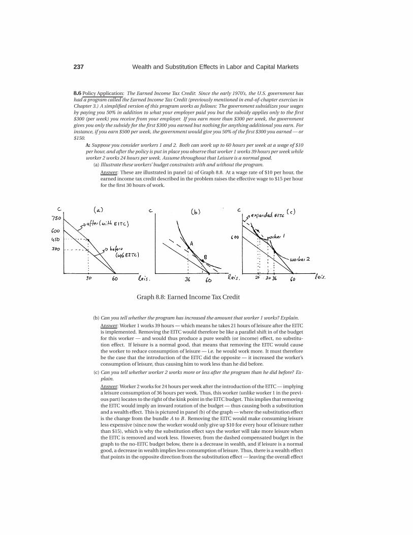
(a) Illustrate these workers’ budget constraints with and without the program.
Answer: These are illustrated in panel (a) of Graph 8.8. At a wage rate of $10 per hour, the
earned income tax credit described in the problem raises the effective wage to $15 per hour
for the first 30 hours of work.
Graph 8.8: Earned Income Tax Credit
(b) Can you tell whether the program has increased the amount that worker 1 works? Explain.
Answer: Worker 1 works 39 hours — which means he takes 21 hours of leisure after the EITC
is implemented. Removing the EITC would therefore be like a parallel shift in of the budget
for this worker — and would thus produce a pure wealth (or income) effect, no substitu-
tion effect. If leisure is a normal good, that means that removing the EITC would cause
the worker to reduce consumption of leisure — i.e. he would work more. It must therefore
be the case that the introduction of the EITC did the opposite — it increased the worker’s
consumption of leisure, thus causing him to work less than he did before.
(c) Can you tell whether worker 2 works more or less after the program than he did before? Ex-
plain.
Answer: Worker 2 works for 24 hours per week after the introduction of the EITC — implying
a leisure consumption of 36 hours per week. Thus, this worker (unlike worker 1 in the previ-
ous part) locates to the right of the kink point in the EITC budget. This implies that removing
the EITC would imply an inward rotation of the budget — thus causing both a substitution
and a wealth effect. This is pictured in panel (b) of the graph — where the substitution effect
is the change from the bundle A to B . Removing the EITC would make consuming leisure
less expensive (since now the worker would only give up $10 for every hour of leisure rather
than $15), which is why the substitution effect says the worker will take more leisure when
the EITC is removed and work less. However, from the dashed compensated budget in the
graph to the no-EITC budget below, there is a decrease in wealth, and if leisure is a normal
good, a decrease in wealth implies less consumption of leisure. Thus, there is a wealth effect
that points in the opposite direction from the substitution effect — leaving the overall effect
Wealth and Substitution Effects in Labor and Capital Markets 238
ambiguous. The more substitutable leisure and consumption are, the more likely it is that
the removal of the EITC would cause the worker to work less. The introduction of the EITC
is of course the mirror image — the more substitutable leisure and consumption are, the
more likely it is that the introduction of the EITC will cause the worker to work more.
(d) Now suppose the government expands the program by raising the cut-off from $300 to $400.
In other words, now the government applies the subsidy to earnings up to $400 per week. Can
you tell whether worker 1 will now work more or less? What about worker 2?
Answer: Panel (c) of the graph illustrates the initial without-EITC budget and the $300 EITC
budget as in panel (a). In addition, the dashed extension of the EITC budget represents
the expanded $400 EITC budget. This extension of the steeper EITC slope has no impact
on worker 2 — worker 2 originally optimized at 36 hours of leisure, and no better bundles
are made available by the expanded budget. Thus, worker 2 would do nothing differently.
Worker 1, on the other hand, is affected by the change in the EITC. He initially takes 21 hours
of leisure — which means the new EITC budget affects him both because it has a different
slope and because it is further out. Since leisure is a normal good, we know the worker will
not choose to optimize on the part of the new budget that lies to the left of the new kink
point (at 20 hours of leisure) — because that would be equivalent to reducing the amount of
leisure when wealth increases. So worker 1 will end up somewhere on the steeper portion
of the new EITC budget — somewhere between 20 hours of leisure and 30 hours of leisure.
We can’t tell exactly where — there are once again offsetting wealth and substitution effects.
The substitution effect says that worker 1 should now consume less leisure (i.e. work more)
because leisure has become more expensive ($15 rather than $10 per hour). The wealth
effect, on the other hand, says the worker is richer and therefore should consume more
leisure (i.e. work less). Either effect may dominate. The more substitutable leisure and
consumption are for the worker, the more likely it is that the worker will work more under
the expanded EITC. The most he will work more, however, is 1 hour.
B: Suppose that workers have tastes over consumption c and leisure ℓ that can be represented by the
function u(c ,ℓ) = cαℓ(1−α).
(a) Given you know which portion of the budget constraint worker 2 ends up on, can you write
down the optimization problem that solves for his optimal choice? Solve the problem and
determine what value α must take for worker 2 in order for him to have chosen to work 24
hours under the EITC program.
Answer: The optimization problem for worker 2 is
maxc,ℓ
cαℓ(1−α) subject to c = 15(60−ℓ). (8.40)
Setting up the Lagrange function and solving the first two first order conditions, we get c =(15αℓ)/(1−α). Plugging this into the budget constraint and solving for ℓ,we get ℓ= 60(1−α),
and plugging this into c = (15αℓ)/(1−α), we get c = 900α.
In order for the worker to choose 24 hours of work and thus 36 hours of leisure, it must then
be that ℓ= 36 = 60(1−α). Solving for α, we get α= 24/60 = 0.4.
(b) Repeat the same for worker 1 — but be sure you specify the budget constraint correctly given
that you know the worker is on a different portion of the EITC budget. (Hint: If you extend the
relevant portion of the budget constraint to the leisure axis, you should find that it intersects
at 75 leisure hours.)
Answer: The optimization problem now would be
maxc,ℓ
cαℓ(1−α) subject to c = 750−10ℓ. (8.41)
Going through the same steps as above, we then get ℓ= 75(1−α) and c = 750α. In order for
this worker to choose 39 hours of work or 21 hours of leisure, it therefore has to be the case
that ℓ= 21 = 75(1−α) or α= 0.72.
(c) Having identified the relevant α parameters for workers 1 and 2, determine whether either of
them works more or less than he would have in the absence of the program.
Answer: In the absence of the EITC program, the workers would solve

239 Wealth and Substitution Effects in Labor and Capital Markets
maxc,ℓ
cαℓ(1−α) subject to c = 10(60−ℓ) (8.42)
which gives ℓ = 60(1−α) and c = 600α. Worker 1 has α = 0.72 — which means he takes
60(1−0.72) = 16.8 hours of leisure without EITC and 21 hours of leisure with the EITC. Thus,
worker 1 works 4.2 hours less under EITC. This is consistent with our intuitive graphs —
where we concluded that the EITC has a pure wealth effect for worker 1 — causing him to
work less. Worker 2 has α = 0.4 — which means he takes 60(1− 0.6) = 36 hours of leisure
before EITC and 36 hours of leisure after EITC. Thus, worker 2 does not change his work
hours as a result of the EITC. This is also consistent with our graphical analysis where we
found competing wealth and substitution effects for worker 2 — effects that exactly offset
each other when the worker has the tastes modeled here.
(d) Determine how each worker would respond to an increase in the EITC cut-off from $300 to
$400.
Answer: We already know from our intuitive analysis that nothing changes for worker 2
— he continues to operate on the steeper portion of the budget defined by the equation
c = 15(60− ℓ) which we used in problem (8.40). Since the problem remains unchanged,
the solution remains unchanged. For worker 1, however, the relevant budget constraint
now is c = 900− 15ℓ (rather than 750− 10ℓ as in problem (8.41)). Thus, since the relevant
constraint has changed, we need to solve the problem with the new constraint — which
gives us ℓ = 60(1−α) = 60(1−0.72) = 16.8 and c = 900α = 900(0.72) = 648. But this would
put him on the steep budget to the right of the kink — which implies the true optimum is at
the kink where ℓ= 20. Thus, he will work 1 hour more.
(e) For what ranges of α would a worker choose the kink-point in the original EITC budget you
drew (i.e. the one with a $300 cutoff)?
Answer: To figure out this range, we need to determine the values of α for which 30 hours
of leisure is optimal for the problems written out in equations (8.40) and (8.41). In other
words, for each of the two budget line segments, what are the values of α for which a worker
would optimize at precisely the kink point. Any α between the values we get from these two
exercises will be such that the kink point is optimal.
For the problem in (8.41), we calculated ℓ= 60(1−α). Setting ℓ equal to 30, we can solve for
α = 0.5. For the problem in (8.40), we calculated ℓ= 75(1−α). Setting ℓ = 30, we can solve
for α = 0.6. Thus, for 0.5 ≤ α ≤ 0.6, the kink point where the worker works for 30 hours a
week is optimal.
Wealth and Substitution Effects in Labor and Capital Markets 240
8.7 Policy Application: Subsidizing Savings versus Taxing Borrowing: In end-of-chapter exercise 6.5 we
analyzed cases where the interest rates for borrowing and saving are different. Part of the reason they
might be different is because of government policy.
A: Suppose banks are currently willing to lend and borrow at the same interest rate. Consider an
individual who has income e1 now and e2 in a future period, with the interest rate over that period
equal to r . After considering the tradeoffs, the individual chooses to borrow on his future income
rather than save. Suppose in this exercise that the individual’s tastes are homothetic.
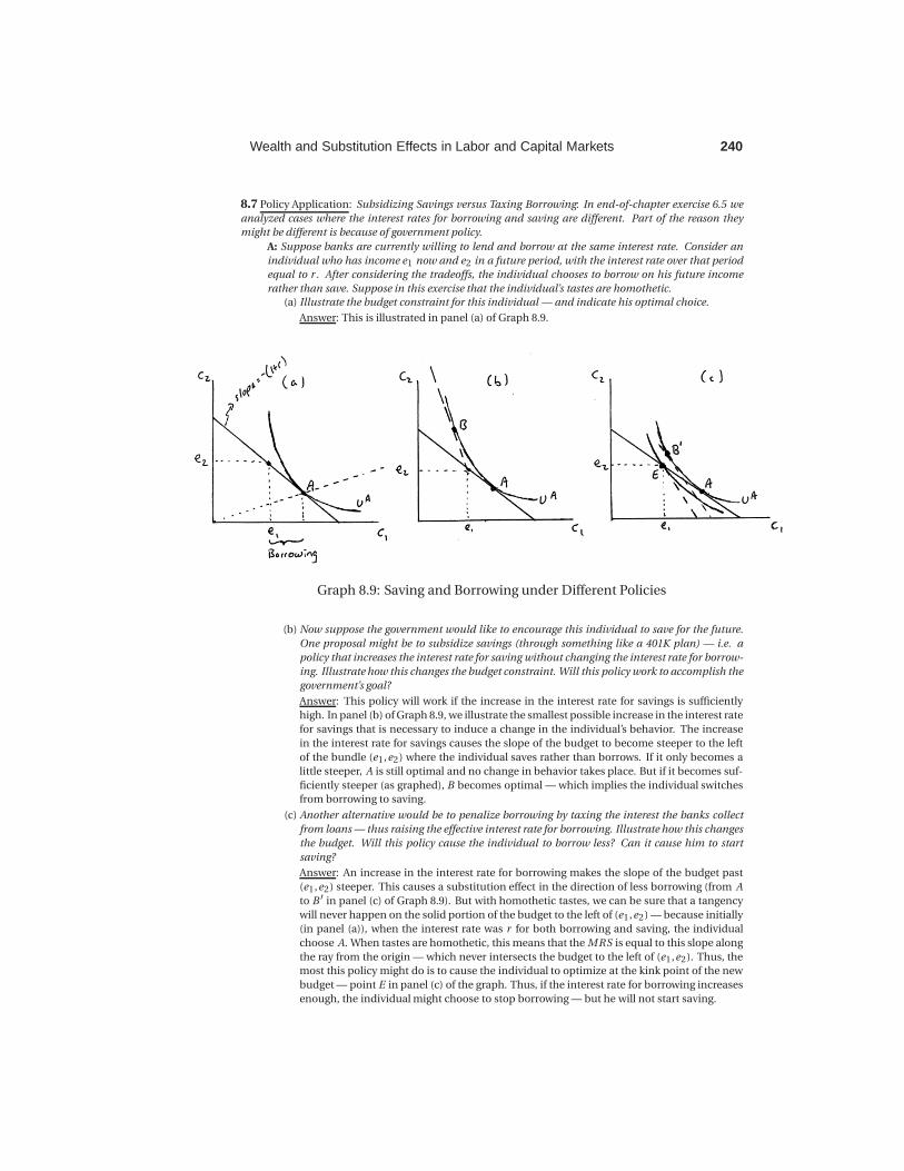
(a) Illustrate the budget constraint for this individual — and indicate his optimal choice.
Answer: This is illustrated in panel (a) of Graph 8.9.
Graph 8.9: Saving and Borrowing under Different Policies
(b) Now suppose the government would like to encourage this individual to save for the future.
One proposal might be to subsidize savings (through something like a 401K plan) — i.e. a
policy that increases the interest rate for saving without changing the interest rate for borrow-
ing. Illustrate how this changes the budget constraint. Will this policy work to accomplish the
government’s goal?
Answer: This policy will work if the increase in the interest rate for savings is sufficiently
high. In panel (b) of Graph 8.9, we illustrate the smallest possible increase in the interest rate
for savings that is necessary to induce a change in the individual’s behavior. The increase
in the interest rate for savings causes the slope of the budget to become steeper to the left
of the bundle (e1,e2) where the individual saves rather than borrows. If it only becomes a
little steeper, A is still optimal and no change in behavior takes place. But if it becomes suf-
ficiently steeper (as graphed), B becomes optimal — which implies the individual switches
from borrowing to saving.
(c) Another alternative would be to penalize borrowing by taxing the interest the banks collect
from loans — thus raising the effective interest rate for borrowing. Illustrate how this changes
the budget. Will this policy cause the individual to borrow less? Can it cause him to start
saving?
Answer: An increase in the interest rate for borrowing makes the slope of the budget past
(e1,e2) steeper. This causes a substitution effect in the direction of less borrowing (from A
to B ′ in panel (c) of Graph 8.9). But with homothetic tastes, we can be sure that a tangency
will never happen on the solid portion of the budget to the left of (e1,e2) — because initially
(in panel (a)), when the interest rate was r for both borrowing and saving, the individual
choose A. When tastes are homothetic, this means that the MRS is equal to this slope along
the ray from the origin — which never intersects the budget to the left of (e1,e2). Thus, the
most this policy might do is to cause the individual to optimize at the kink point of the new
budget — point E in panel (c) of the graph. Thus, if the interest rate for borrowing increases
enough, the individual might choose to stop borrowing — but he will not start saving.
241 Wealth and Substitution Effects in Labor and Capital Markets
(d) In reality, the government often does the opposite of these two policies: Savings (outside qual-
ified retirement plans) are taxed while some forms of borrowing (in particular borrowing to
buy a home) are subsidized. Suppose again that initially the interest rate for borrowing and
saving is the same — and then suppose that the combination of taxes on savings (which low-
ers the effective interest rate on savings) and subsidies for borrowing (which lowers the effec-
tive interest rate for borrowing) reduce the interest rate to r ′ < r equally for both saving and
borrowing. How will this individual respond to this combination of policies?
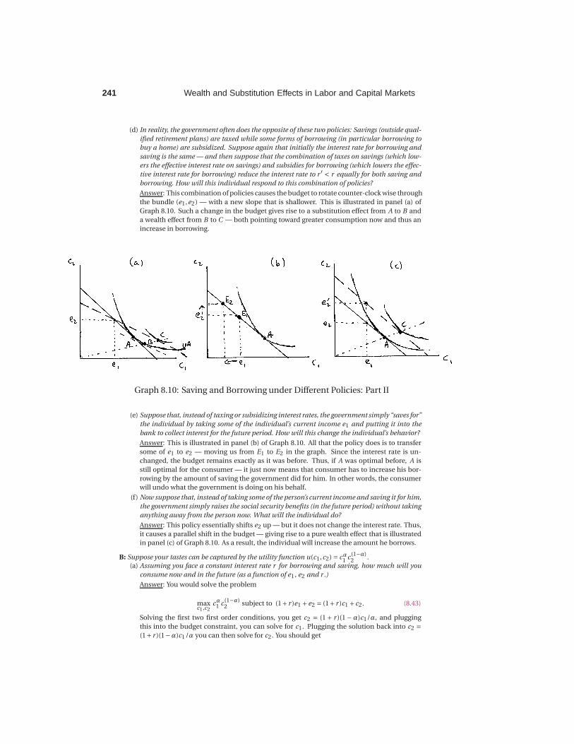
Answer: This combination of policies causes the budget to rotate counter-clock wise through
the bundle (e1,e2) — with a new slope that is shallower. This is illustrated in panel (a) of
Graph 8.10. Such a change in the budget gives rise to a substitution effect from A to B and
a wealth effect from B to C — both pointing toward greater consumption now and thus an
increase in borrowing.
Graph 8.10: Saving and Borrowing under Different Policies: Part II
(e) Suppose that, instead of taxing or subsidizing interest rates, the government simply “saves for”
the individual by taking some of the individual’s current income e1 and putting it into the
bank to collect interest for the future period. How will this change the individual’s behavior?
Answer: This is illustrated in panel (b) of Graph 8.10. All that the policy does is to transfer
some of e1 to e2 — moving us from E1 to E2 in the graph. Since the interest rate is un-
changed, the budget remains exactly as it was before. Thus, if A was optimal before, A is
still optimal for the consumer — it just now means that consumer has to increase his bor-
rowing by the amount of saving the government did for him. In other words, the consumer
will undo what the government is doing on his behalf.
(f) Now suppose that, instead of taking some of the person’s current income and saving it for him,
the government simply raises the social security benefits (in the future period) without taking
anything away from the person now. What will the individual do?
Answer: This policy essentially shifts e2 up — but it does not change the interest rate. Thus,
it causes a parallel shift in the budget — giving rise to a pure wealth effect that is illustrated
in panel (c) of Graph 8.10. As a result, the individual will increase the amount he borrows.
B: Suppose your tastes can be captured by the utility function u(c1,c2) = cα1
c(1−α)2
.
(a) Assuming you face a constant interest rate r for borrowing and saving, how much will you
consume now and in the future (as a function of e1, e2 and r .)
Answer: You would solve the problem
maxc1,c2
cα1 c(1−α)2 subject to (1+ r )e1 +e2 = (1+ r )c1 +c2. (8.43)
Solving the first two first order conditions, you get c2 = (1 + r )(1 −α)c1/α, and plugging
this into the budget constraint, you can solve for c1. Plugging the solution back into c2 =(1+ r )(1−α)c1 /α you can then solve for c2. You should get
Wealth and Substitution Effects in Labor and Capital Markets 242
c1 =α[(1+ r )e1 +e2]
(1+ r )and c2 = (1−α)[(1+ r )e1 +e2]. (8.44)
(b) For what values of α will you choose to borrow rather than save?
Answer: In order for you to borrow, it must be that your optimal c1 is greater than your
current income e1 — i.e. c1 > e1. Using the optimal c1 just derived above, this implies
α[(1+ r )e1 +e2]
(1+ r )> e1. (8.45)
Solving for α, we get that
α>(1+ r )e1
e1(1+ r )+e2. (8.46)
(c) Suppose that α = 0.5, e1 = 100,000, e2 = 125,000 and r = 0.10. How much do you save or
borrow?
Answer: Using our solutions in equation (8.44), we get c1 = $106,818.18 and c2 = $117,500.
Thus, you would borrow $6,818.
(d) If the government could come up with a “financial literacy” course that changes how you view
the tradeoff between now and the future by impacting α, how much would this program have
to change your α in order to get you to stop borrowing?
Answer: Using equation (8.46), α = 0.4681 would be necessary in order for you to neither
borrow nor save. For α greater than that, you would continue to borrow.
(e) Suppose the “financial literacy” program had no impact on α. How much would the govern-
ment have to raise the interest rate for saving (as described in A(b)) in order for you to become
a saver? (Hint: You need to first determine c1 and c2 as a function of just r . You can then
determine the utility you receive as a function of just r — and you will not switch to saving
until r is sufficiently high to give you the same utility you get by borrowing.)
Answer: Using our answers from above, the utility you get from borrowing is
u(106818.18,117500) = 106818.180.5 1175000.5 ≈ 112,031.85. (8.47)
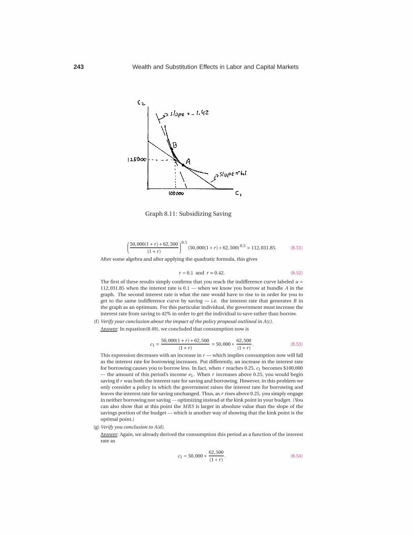
Put differently, the label on the indifference curve that you end up at if you borrow is 112,031.85.
This indifference curve, and the optimal bundle when you borrow, is illustrated as point A
in Graph 8.11.
We know that, as the interest rate for savings goes up, the budget to the left of (e1,e2) =(100000,125000) increases. To find how much the government must subsidize the inter-
est rate in order to cause you to switch from borrowing to saving, we have to determine
the interest rate that makes this steeper budget tangent to the same indifference curve that
contains A — i.e. the indifference curve with utility 112,031.85.
With e1 = 100,000, e2 = 125,000 and α= 1/2, equation (8.44) tells us you will consume
c1 =100000(1+ r )+125000
2(1+ r )and c2 =
[100000(1+ r )+125000]
2(8.48)
for any given interest rate r . This can also be written
c1 =50,000(1+ r )+62,500
(1+ r )and c2 = 50,000(1+ r )+62,500. (8.49)
Using the results from equation (8.49), the utility you get at interest rate r is then
u(c1,c2) =(
50,000(1+ r )+62,500
(1+ r )
)0.5
(50,000(1+ r )+62,500) 0.5 . (8.50)
Thus, to solve for the interest rate r that gets the same utility as the utility you currently get
by borrowing, we have to solve
243 Wealth and Substitution Effects in Labor and Capital Markets
Graph 8.11: Subsidizing Saving
(50,000(1+ r )+62,500
(1+ r )
)0.5
(50,000(1+ r )+62,500) 0.5 = 112,031.85. (8.51)
After some algebra and after applying the quadratic formula, this gives
r = 0.1 and r ≈ 0.42. (8.52)
The first of these results simply confirms that you reach the indifference curve labeled u =112,031.85 when the interest rate is 0.1 — when we know you borrow at bundle A in the
graph. The second interest rate is what the rate would have to rise to in order for you to
get to the same indifference curve by saving — i.e. the interest rate that generates B in
the graph as an optimum. For this particular individual, the government must increase the
interest rate from saving to 42% in order to get the individual to save rather than borrow.
(f) Verify your conclusion about the impact of the policy proposal outlined in A(c).
Answer: In equation(8.49), we concluded that consumption now is
c1 =50,000(1+ r )+62,500
(1+ r )= 50,000+
62,500
(1+ r ). (8.53)
This expression decreases with an increase in r — which implies consumption now will fall
as the interest rate for borrowing increases. Put differently, an increase in the interest rate
for borrowing causes you to borrow less. In fact, when r reaches 0.25, c1 becomes $100,000
— the amount of this period’s income e1. When r increases above 0.25, you would begin
saving if r was both the interest rate for saving and borrowing. However, in this problem we
only consider a policy in which the government raises the interest rate for borrowing and
leaves the interest rate for saving unchanged. Thus, as r rises above 0.25, you simply engage
in neither borrowing nor saving — optimizing instead at the kink point in your budget. (You
can also show that at this point the MRS is larger in absolute value than the slope of the
savings portion of the budget — which is another way of showing that the kink point is the
optimal point.)
(g) Verify you conclusion to A(d).
Answer: Again, we already derived the consumption this period as a function of the interest
rate as
c1 = 50,000+62,500
(1+ r ). (8.54)

Wealth and Substitution Effects in Labor and Capital Markets 244
A decrease in the general interest rate for both saving and borrowing will thus increase c1.
Thus, you will increase your borrowing under these policies.
(h) Verify your conclusion to A(e); i.e. suppose the government takes x of your current income e1
and saves it — thus increasing e2 by x(1+ r ).
Answer: The original budget constraint (1 + r )e1 + e2 = (1 + r )c1 + c2 is thus changed to
(1+ r )(e1 −x)+ (e2 + (1+ r )x) = (1+ r )c1 +c2. The left hand side of the latter reduces to the
left hand side of the former — thus the budget constraint remains the same. With the same
budget constraint, the optimal choice remains unchanged.
(i) Finally, suppose the increase in social security benefits outlined in A(f) is implemented; i.e.
suppose e2 is increased by x. How and by how much does your borrowing change?
Answer: In equation (8.44), we determined
c1 =α[(1+ r )e1 +e2]
(1+ r ). (8.55)
An increase in e2 by x causes an increase in consumption c1 by αx/(1+ r ) — which implies
an increase in borrowing by that amount.
245 Wealth and Substitution Effects in Labor and Capital Markets
8.8 Policy Application: Tax Revenues and the Laffer Curve: In this exercise, we will consider how the tax
rate on wages relates to the amount of tax revenue collected.
A: As introduced in Section B, the Laffer Curve depicts the relationship between the tax rate on the
horizontal axis and tax revenues on the vertical. (See the footnote in Section 8B.2.2 for background
on the origins of the name of this curve.) Because people’s decision on how much to work may be
affected by the tax rate, deriving this relationship is not as straightforward as many think.
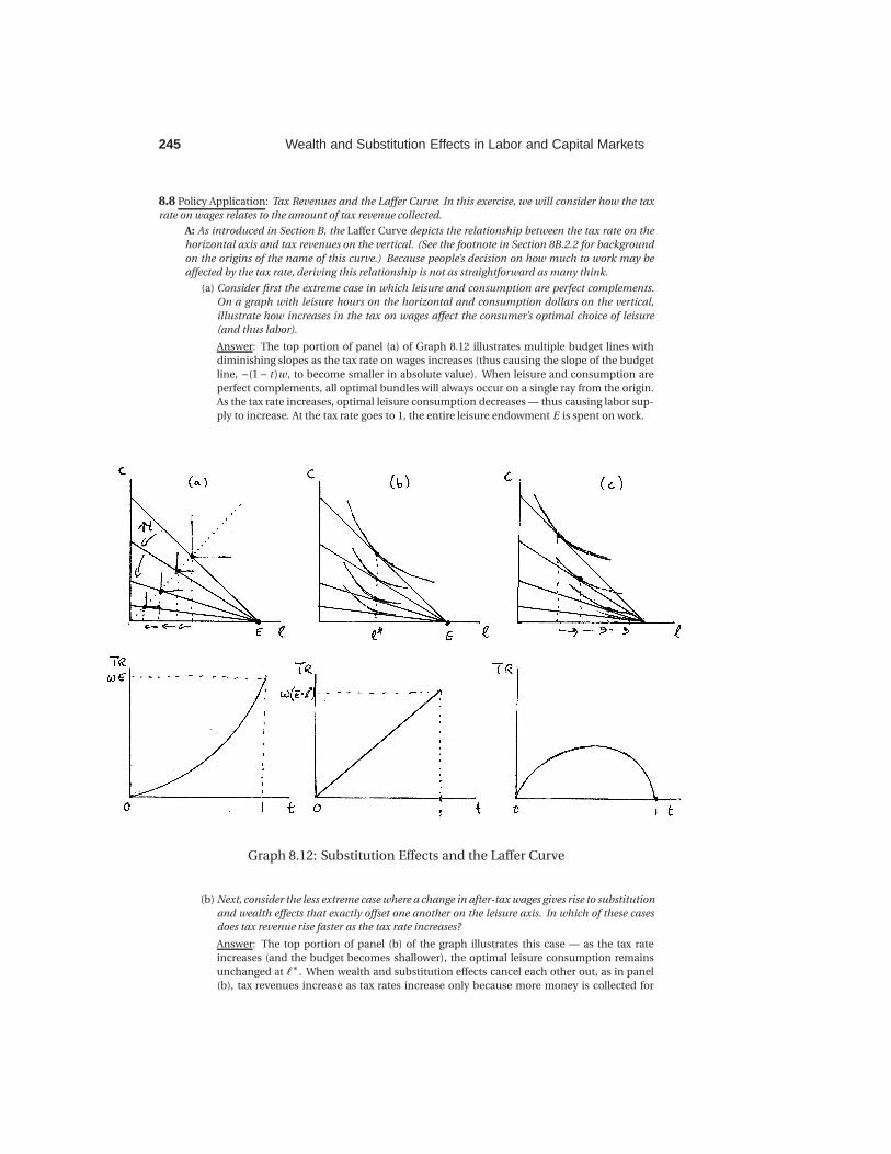
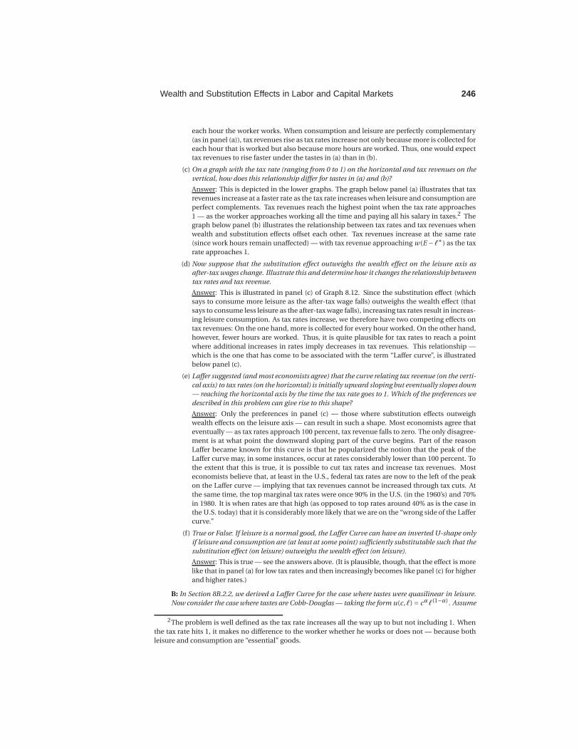
(a) Consider first the extreme case in which leisure and consumption are perfect complements.
On a graph with leisure hours on the horizontal and consumption dollars on the vertical,
illustrate how increases in the tax on wages affect the consumer’s optimal choice of leisure
(and thus labor).
Answer: The top portion of panel (a) of Graph 8.12 illustrates multiple budget lines with
diminishing slopes as the tax rate on wages increases (thus causing the slope of the budget
line, −(1− t )w , to become smaller in absolute value). When leisure and consumption are
perfect complements, all optimal bundles will always occur on a single ray from the origin.
As the tax rate increases, optimal leisure consumption decreases — thus causing labor sup-
ply to increase. At the tax rate goes to 1, the entire leisure endowment E is spent on work.
Graph 8.12: Substitution Effects and the Laffer Curve
(b) Next, consider the less extreme case where a change in after-tax wages gives rise to substitution
and wealth effects that exactly offset one another on the leisure axis. In which of these cases
does tax revenue rise faster as the tax rate increases?
Answer: The top portion of panel (b) of the graph illustrates this case — as the tax rate
increases (and the budget becomes shallower), the optimal leisure consumption remains
unchanged at ℓ∗. When wealth and substitution effects cancel each other out, as in panel
(b), tax revenues increase as tax rates increase only because more money is collected for
Wealth and Substitution Effects in Labor and Capital Markets 246
each hour the worker works. When consumption and leisure are perfectly complementary
(as in panel (a)), tax revenues rise as tax rates increase not only because more is collected for
each hour that is worked but also because more hours are worked. Thus, one would expect
tax revenues to rise faster under the tastes in (a) than in (b).
(c) On a graph with the tax rate (ranging from 0 to 1) on the horizontal and tax revenues on the
vertical, how does this relationship differ for tastes in (a) and (b)?
Answer: This is depicted in the lower graphs. The graph below panel (a) illustrates that tax
revenues increase at a faster rate as the tax rate increases when leisure and consumption are
perfect complements. Tax revenues reach the highest point when the tax rate approaches
1 — as the worker approaches working all the time and paying all his salary in taxes.2 The
graph below panel (b) illustrates the relationship between tax rates and tax revenues when
wealth and substitution effects offset each other. Tax revenues increase at the same rate
(since work hours remain unaffected) — with tax revenue approaching w(E −ℓ∗) as the tax
rate approaches 1.
(d) Now suppose that the substitution effect outweighs the wealth effect on the leisure axis as
after-tax wages change. Illustrate this and determine how it changes the relationship between
tax rates and tax revenue.
Answer: This is illustrated in panel (c) of Graph 8.12. Since the substitution effect (which
says to consume more leisure as the after-tax wage falls) outweighs the wealth effect (that
says to consume less leisure as the after-tax wage falls), increasing tax rates result in increas-
ing leisure consumption. As tax rates increase, we therefore have two competing effects on
tax revenues: On the one hand, more is collected for every hour worked. On the other hand,
however, fewer hours are worked. Thus, it is quite plausible for tax rates to reach a point
where additional increases in rates imply decreases in tax revenues. This relationship —
which is the one that has come to be associated with the term “Laffer curve”, is illustrated
below panel (c).
(e) Laffer suggested (and most economists agree) that the curve relating tax revenue (on the verti-
cal axis) to tax rates (on the horizontal) is initially upward sloping but eventually slopes down
— reaching the horizontal axis by the time the tax rate goes to 1. Which of the preferences we
described in this problem can give rise to this shape?
Answer: Only the preferences in panel (c) — those where substitution effects outweigh
wealth effects on the leisure axis — can result in such a shape. Most economists agree that
eventually — as tax rates approach 100 percent, tax revenue falls to zero. The only disagree-
ment is at what point the downward sloping part of the curve begins. Part of the reason
Laffer became known for this curve is that he popularized the notion that the peak of the
Laffer curve may, in some instances, occur at rates considerably lower than 100 percent. To
the extent that this is true, it is possible to cut tax rates and increase tax revenues. Most
economists believe that, at least in the U.S., federal tax rates are now to the left of the peak
on the Laffer curve — implying that tax revenues cannot be increased through tax cuts. At
the same time, the top marginal tax rates were once 90% in the U.S. (in the 1960’s) and 70%
in 1980. It is when rates are that high (as opposed to top rates around 40% as is the case in
the U.S. today) that it is considerably more likely that we are on the “wrong side of the Laffer
curve.”
(f) True or False: If leisure is a normal good, the Laffer Curve can have an inverted U-shape only
if leisure and consumption are (at least at some point) sufficiently substitutable such that the
substitution effect (on leisure) outweighs the wealth effect (on leisure).
Answer: This is true — see the answers above. (It is plausible, though, that the effect is more
like that in panel (a) for low tax rates and then increasingly becomes like panel (c) for higher
and higher rates.)
B: In Section 8B.2.2, we derived a Laffer Curve for the case where tastes were quasilinear in leisure.
Now consider the case where tastes are Cobb-Douglas — taking the form u(c ,ℓ) = cαℓ(1−α). Assume
2The problem is well defined as the tax rate increases all the way up to but not including 1. When
the tax rate hits 1, it makes no difference to the worker whether he works or does not — because both
leisure and consumption are “essential” goods.

247 Wealth and Substitution Effects in Labor and Capital Markets
that a worker has 60 hours of weekly leisure endowment that he can sell in the labor market for wage
w.
(a) Suppose the worker’s wages are taxed at a rate t . Derive his optimal leisure choice.
Answer: We need to solve
maxc,ℓ
cαℓ(1−α) subject to c = (1− t )w(60−ℓ). (8.56)
Solving this in the usual way, we get ℓ= 60(1−α).
(b) For someone with these tastes, does the Laffer Curve take the inverted U-shape described in
Section 8B.2.2. Why or why not? Which of the cases described in A does this represent?
Answer: We just derived that ℓ= 60(1−α) — which means that the number of weekly hours
worked is equal to 60α. Thus, work hours are not impacted by the tax rate t — which means
substitution and wealth effects exactly offset each other as in the case described in A(b). The
relationship between tax rates t and tax revenues T R is then quite straightforward:
T R = w(60α)t , (8.57)
which has the shape depicted in the lower graph of panel (b) in Graph 8.12, a straight line
with intercept of zero and slope w(60α).
(c) Now consider the more general CES function (αc−ρ + (1−α)ℓ−ρ )−1/ρ . Again derive the opti-
mal leisure consumption.
Answer: We now need to solve the problem
maxc,ℓ
(αc−ρ + (1−α)ℓ−ρ
)−1/ρsubject to c = (1− t )w(60−ℓ). (8.58)
The usual first two first order conditions simplify to
c =(α(1− t )w
(1−α)
)1/(ρ+1)
ℓ. (8.59)
Substituting this into the budget constraint c = (1− t )w(60−ℓ), we get
ℓ=60(1− t )w
(α(1−t )w
(1−α)
)1/(ρ+1)+ (1− t )w
= 60
[(α
(1−α)
)1/(ρ+1)
((1− t )w)−ρ/(ρ+1) +1
]−1
. (8.60)
(d) Does your answer simplify to what you would expect when ρ = 0?
Answer When ρ = 0, equation (8.60) reduces to
ℓ= 60
[(α
(1−α)
)1
((1− t )w)0 +1
]−1
= 60
[(α
(1−α)
)+1
]−1
= 60(1−α). (8.61)
This is exactly what we derived for the Cobb-Douglas tastes in (a) — which makes sense
since CES utility functions become Cobb-Douglas when ρ approaches 0.
(e) Determine the range of values of ρ such that leisure consumption increases with t .
Answer: We are interested in the change in ℓ with a change in t — i.e. we are interested in
the derivative of ℓ in equation (8.60) with respect to t . This derivative is
∂ℓ
∂t=−60
[(α
(1−α)
) 1ρ+1
((1− t )w)− ρ
ρ+1 +1
]−2 ( −ρ(ρ+1)
)(α
(1−α)
) 1ρ+1
((1− t )w)− 2ρ+1
ρ+1 (−w).
(8.62)
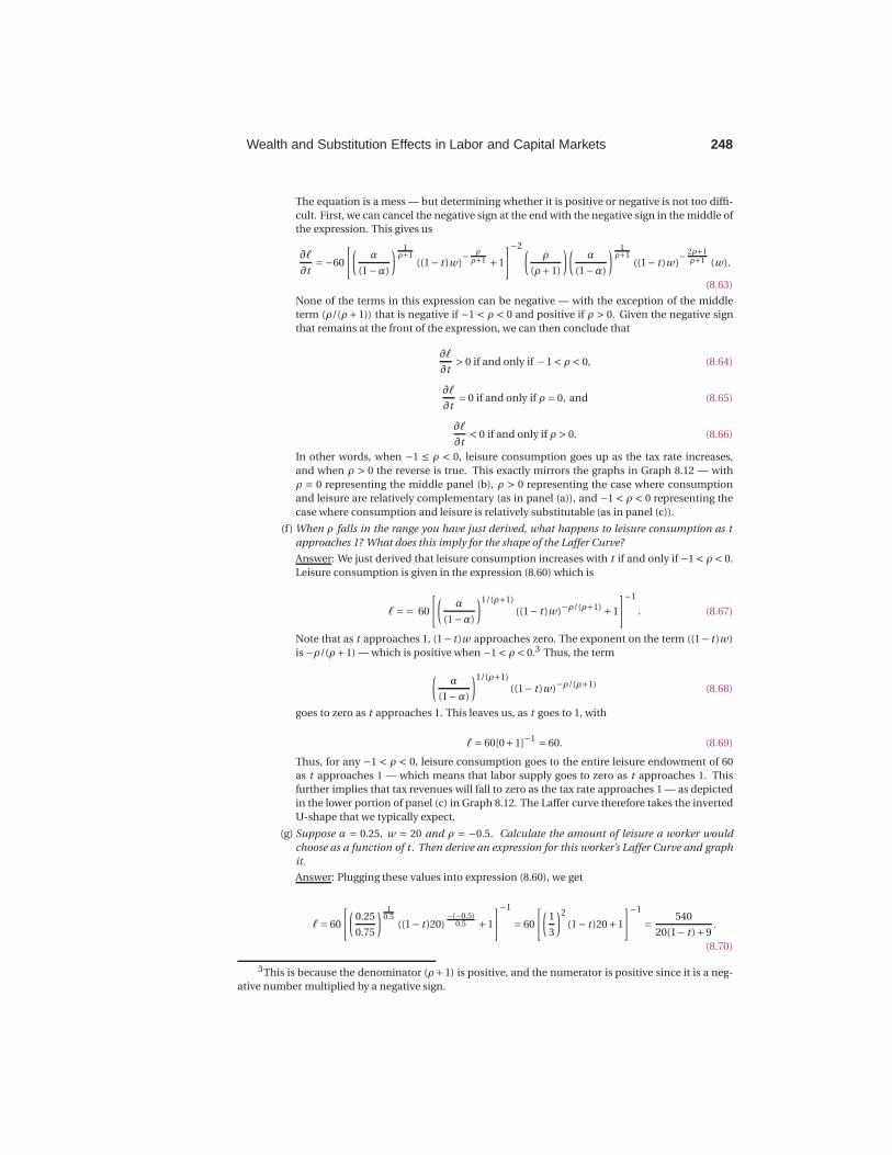
Wealth and Substitution Effects in Labor and Capital Markets 248
The equation is a mess — but determining whether it is positive or negative is not too diffi-
cult. First, we can cancel the negative sign at the end with the negative sign in the middle of
the expression. This gives us
∂ℓ
∂t=−60
[(α
(1−α)
) 1ρ+1
((1− t )w)− ρ
ρ+1 +1
]−2 (ρ
(ρ+1)
)(α
(1−α)
) 1ρ+1
((1− t )w)− 2ρ+1
ρ+1 (w).
(8.63)
None of the terms in this expression can be negative — with the exception of the middle
term (ρ/(ρ+1)) that is negative if −1 < ρ < 0 and positive if ρ > 0. Given the negative sign
that remains at the front of the expression, we can then conclude that
∂ℓ
∂t> 0 if and only if −1 < ρ < 0, (8.64)
∂ℓ
∂t= 0 if and only if ρ = 0, and (8.65)
∂ℓ
∂t< 0 if and only if ρ > 0. (8.66)
In other words, when −1 ≤ ρ < 0, leisure consumption goes up as the tax rate increases,
and when ρ > 0 the reverse is true. This exactly mirrors the graphs in Graph 8.12 — with
ρ = 0 representing the middle panel (b), ρ > 0 representing the case where consumption
and leisure are relatively complementary (as in panel (a)), and −1 < ρ < 0 representing the
case where consumption and leisure is relatively substitutable (as in panel (c)).
(f) When ρ falls in the range you have just derived, what happens to leisure consumption as t
approaches 1? What does this imply for the shape of the Laffer Curve?
Answer: We just derived that leisure consumption increases with t if and only if −1 < ρ < 0.
Leisure consumption is given in the expression (8.60) which is
ℓ== 60
[(α
(1−α)
)1/(ρ+1)
((1− t )w)−ρ/(ρ+1) +1
]−1
. (8.67)
Note that as t approaches 1, (1− t )w approaches zero. The exponent on the term ((1− t )w)
is −ρ/(ρ+1) — which is positive when −1 < ρ < 0.3 Thus, the term
(α
(1−α)
)1/(ρ+1)
((1− t )w)−ρ/(ρ+1) (8.68)
goes to zero as t approaches 1. This leaves us, as t goes to 1, with
ℓ= 60[0+1]−1 = 60. (8.69)
Thus, for any −1 < ρ < 0, leisure consumption goes to the entire leisure endowment of 60
as t approaches 1 — which means that labor supply goes to zero as t approaches 1. This
further implies that tax revenues will fall to zero as the tax rate approaches 1 — as depicted
in the lower portion of panel (c) in Graph 8.12. The Laffer curve therefore takes the inverted
U-shape that we typically expect.
(g) Suppose α = 0.25, w = 20 and ρ = −0.5. Calculate the amount of leisure a worker would
choose as a function of t . Then derive an expression for this worker’s Laffer Curve and graph
it.
Answer: Plugging these values into expression (8.60), we get
ℓ= 60
[(0.25
0.75
) 10.5
((1− t )20)−(−0.5)
0.5 +1
]−1
= 60
[(1
3
)2
(1− t )20+1
]−1
=540
20(1− t )+9.
(8.70)
3This is because the denominator (ρ+1) is positive, and the numerator is positive since it is a neg-
ative number multiplied by a negative sign.
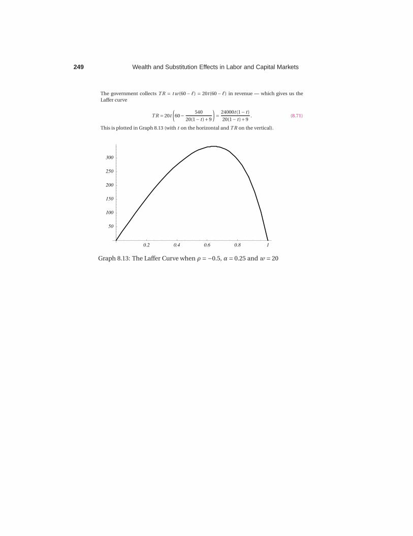
249 Wealth and Substitution Effects in Labor and Capital Markets
The government collects T R = t w(60− ℓ) = 20t (60− ℓ) in revenue — which gives us the
Laffer curve
T R = 20t
(60−
540
20(1− t )+9
)=
24000t (1− t )
20(1− t )+9. (8.71)
This is plotted in Graph 8.13 (with t on the horizontal and T R on the vertical).
0.2 0.4 0.6 0.8 1
50
100
150
200
250
300
Graph 8.13: The Laffer Curve when ρ =−0.5, α= 0.25 and w = 20
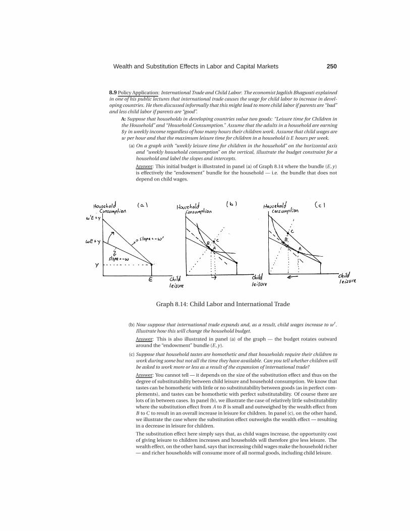
Wealth and Substitution Effects in Labor and Capital Markets 250
8.9 Policy Application: International Trade and Child Labor: The economist Jagdish Bhagwati explained
in one of his public lectures that international trade causes the wage for child labor to increase in devel-
oping countries. He then discussed informally that this might lead to more child labor if parents are “bad”
and less child labor if parents are “good”.
A: Suppose that households in developing countries value two goods: “Leisure time for Children in
the Household” and “Household Consumption.” Assume that the adults in a household are earning
$y in weekly income regardless of how many hours their children work. Assume that child wages are
w per hour and that the maximum leisure time for children in a household is E hours per week.
(a) On a graph with “weekly leisure time for children in the household” on the horizontal axis
and “weekly household consumption” on the vertical, illustrate the budget constraint for a
household and label the slopes and intercepts.
Answer: This initial budget is illustrated in panel (a) of Graph 8.14 where the bundle (E , y)
is effectively the “endowment” bundle for the household — i.e. the bundle that does not
depend on child wages.
Graph 8.14: Child Labor and International Trade
(b) Now suppose that international trade expands and, as a result, child wages increase to w ′.Illustrate how this will change the household budget.
Answer: This is also illustrated in panel (a) of the graph — the budget rotates outward
around the “endowment” bundle (E , y).
(c) Suppose that household tastes are homothetic and that households require their children to
work during some but not all the time they have available. Can you tell whether children will
be asked to work more or less as a result of the expansion of international trade?
Answer: You cannot tell — it depends on the size of the substitution effect and thus on the
degree of substitutability between child leisure and household consumption. We know that
tastes can be homothetic with little or no substitutability between goods (as in perfect com-
plements), and tastes can be homothetic with perfect substitutability. Of course there are
lots of in between cases. In panel (b), we illustrate the case of relatively little substitutability
where the substitution effect from A to B is small and outweighed by the wealth effect from
B to C to result in an overall increase in leisure for children. In panel (c), on the other hand,
we illustrate the case where the substitution effect outweighs the wealth effect — resulting
in a decrease in leisure for children.
The substitution effect here simply says that, as child wages increase, the opportunity cost
of giving leisure to children increases and households will therefore give less leisure. The
wealth effect, on the other hand, says that increasing child wages make the household richer
— and richer households will consume more of all normal goods, including child leisure.
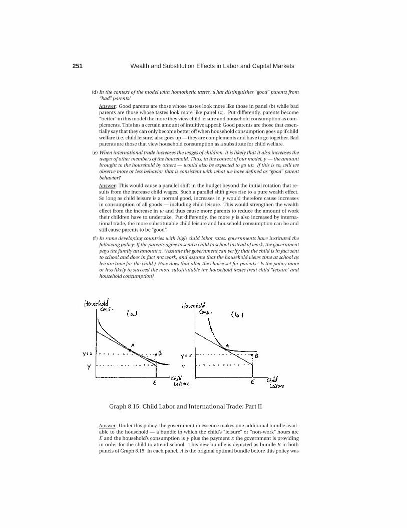
251 Wealth and Substitution Effects in Labor and Capital Markets
(d) In the context of the model with homothetic tastes, what distinguishes “good” parents from
“bad” parents?
Answer: Good parents are those whose tastes look more like those in panel (b) while bad
parents are those whose tastes look more like panel (c). Put differently, parents become
“better” in this model the more they view child leisure and household consumption as com-
plements. This has a certain amount of intuitive appeal: Good parents are those that essen-
tially say that they can only become better off when household consumption goes up if child
welfare (i.e. child leisure) also goes up — they are complements and have to go together. Bad
parents are those that view household consumption as a substitute for child welfare.
(e) When international trade increases the wages of children, it is likely that it also increases the
wages of other members of the household. Thus, in the context of our model, y — the amount
brought to the household by others — would also be expected to go up. If this is so, will we
observe more or less behavior that is consistent with what we have defined as “good” parent
behavior?
Answer: This would cause a parallel shift in the budget beyond the initial rotation that re-
sults from the increase child wages. Such a parallel shift gives rise to a pure wealth effect.
So long as child leisure is a normal good, increases in y would therefore cause increases
in consumption of all goods — including child leisure. This would strengthen the wealth
effect from the increase in w and thus cause more parents to reduce the amount of work
their children have to undertake. Put differently, the more y is also increased by interna-
tional trade, the more substitutable child leisure and household consumption can be and
still cause parents to be “good”.
(f) In some developing countries with high child labor rates, governments have instituted the
following policy: If the parents agree to send a child to school instead of work, the government
pays the family an amount x. (Assume the government can verify that the child is in fact sent
to school and does in fact not work, and assume that the household views time at school as
leisure time for the child.) How does that alter the choice set for parents? Is the policy more
or less likely to succeed the more substitutable the household tastes treat child “leisure” and
household consumption?
Graph 8.15: Child Labor and International Trade: Part II
Answer: Under this policy, the government in essence makes one additional bundle avail-
able to the household — a bundle in which the child’s “leisure” or “non-work” hours are
E and the household’s consumption is y plus the payment x the government is providing
in order for the child to attend school. This new bundle is depicted as bundle B in both
panels of Graph 8.15. In each panel, A is the original optimal bundle before this policy was
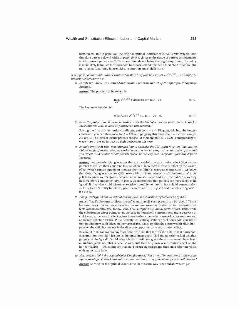
Wealth and Substitution Effects in Labor and Capital Markets 252
introduced. But in panel (a), the original optimal indifference curve is relatively flat and
therefore passes below B while in panel (b) it is closer to the shape of perfect complements
which makes it pass above B . Thus, conditional on A being the original optimum, the policy
is more likely to induce the household to choose B (and thus send their child to school) the
more substitutable are household consumption and child leisure.
B: Suppose parental tastes can be captured by the utility function u(c ,ℓ) = c0.5ℓ0.5. For simplicity,
suppose further that y = 0.
(a) Specify the parents’ constrained optimization problem and set up the appropriate Lagrange
function.
Answer: The problem to be solved is
maxc,ℓ
c0.5ℓ0.5 subject to c = w(E −ℓ). (8.72)
The Lagrange function is
L (c ,ℓ,λ) = c0.5ℓ0.5 +λ(w(E −ℓ)−c). (8.73)
(b) Solve the problem you have set up to determine the level of leisure the parents will choose for
their children. Does w have any impact on this decision?
Solving the first two first order conditions, you get c = wℓ. Plugging this into the budget
constraint, you can then solve for ℓ = E/2 and plugging this back into c = wℓ, you can get
c = wE/2. The level of leisure parents choose for their children (ℓ= E/2) is independent of
wage — so w has no impact on their decision in this case.
(c) Explain intuitively what you have just found. Consider the CES utility function (that has the
Cobb-Douglas function you just worked with as a special case). For what ranges of ρ would
you expect us to be able to call parents “good” in the way that Bhagwati informally defined
the term?
Answer: For the Cobb-Douglas tastes that are modeled, the substitution effect (that causes
parents to reduce their children’s leisure when w increases) is exactly offset by the wealth
effect (which causes parents to increase their children’s leisure as w increases). We know
that Cobb-Douglas tastes are CES tastes with ρ = 0 and elasticity of substitution of 1. As
ρ falls below zero, the goods become more substitutable and as ρ rises above zero they
become more complementary. In part A we determined that parents are more likely to be
“good” if they view child leisure as relatively complementary to household consumption
— thus, for CES utility functions, parents are “bad” if −1 ≤ ρ < 0 and parents are “good” if
0 < ρ ≤∞.
(d) Can parents for whom household consumption is a quasilinear good ever be “good”?
Anwer: Yes, if substitution effects are sufficiently small, such parents can be “good”. This is
because tastes that are quasilinear in consumption would only give rise to substitution ef-
fects with no wealth effect for household consumption (i.e. on the vertical axis). Thus, while
the substitution effect points to an increase in household consumption and a decrease in
child leisure, the wealth effect points to no further change in household consumption and
an increase in child leisure. Put differently, while the quasilinearity of household consump-
tion implies no wealth effect on the vertical axis, it also implies the entire wealth effect hap-
pens on the child leisure axis in the direction opposite to the substitution effect.
Be careful in this answer to pay attention to the fact that the question states that household
consumption, not child leisure, is the quasilinear good. Had the question asked whether
parents can be “good” if child leisure is the quasilinear good, the answer would have been
an unambiguous no. This is because we would then only have a substitution effect on the
horizontal axis — which implies that child leisure decreases and thus child labor increases
with an increase in w .
(e) Now suppose (with the original Cobb-Douglas tastes) that y > 0. If international trade pushes
up the earnings of other household members — thus raising y, what happens to child leisure?
Answer: Solving for the optimal leisure time (in the same way as we did above), we get

253 Wealth and Substitution Effects in Labor and Capital Markets
ℓ=wE + y
2w. (8.74)
The derivative of this with respect to y is positive — i.e. as y increases, so does the amount
of leisure chosen for the child.
(f) Suppose again that y = 0 and the government introduces the policy described in part A(f).
How large does x have to be in order to cause our household to send their child to school
(assuming again that the household views the child’s time at school as leisure time for the
child)?
Answer: Without participating in the policy, the household consumes c = wE/2 and ℓ= E/2
— and therefore gets utility (wE/2)0.5 (E/2)0.5 = w0.5E/2. If the household participates in
the policy, it’s child would get leisure of E and the household consumption would be x.
Thus, participating in the policy means utility of x0.5E0.5. The household will be indifferent
between the two options if the utility of participating and not participating are equal; i.e. if
w0.5E
2= x0.5E0.5. (8.75)
Solving this for x we get x = wE/4. For any x greater than this, the household is therefore
better off choosing to send their child to school.
(g) Using your answer to the previous part, put into words what fraction of the market value of
the child’s time the government has to provide in x in order for the family to choose schooling
over work for their child?
Answer: We concluded above that x has to be at least wE/4 in order for the household to be
willing to send the child to school. The market value of the child’s time endowment is wE .
The amount that is required for the child to be sent to school is therefore equivalent to one
quarter of the market value of the leisure time of the child.
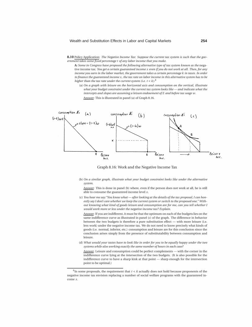
Wealth and Substitution Effects in Labor and Capital Markets 254
8.10 Policy Application: The Negative Income Tax: Suppose the current tax system is such that the gov-
ernment takes some fixed percentage t of any labor income that you make.
A: Some in Congress have proposed the following alternative type of tax system known as the nega-
tive income tax: You get a certain guaranteed income x even if you do not work at all. Then, for any
income you earn in the labor market, the government takes a certain percentage k in taxes. In order
to finance the guaranteed income x, the tax rate on labor income in this alternative system has to be
higher than the tax rate under the current system (i.e. t < k).4
(a) On a graph with leisure on the horizontal axis and consumption on the vertical, illustrate
what your budget constraint under the current tax system looks like — and indicate what the
intercepts and slopes are assuming a leisure endowment of E and before tax wage w.
Answer: This is illustrated in panel (a) of Graph 8.16.
Graph 8.16: Work and the Negative Income Tax
(b) On a similar graph, illustrate what your budget constraint looks like under the alternative
system.
Answer: This is done in panel (b) where, even if the person does not work at all, he is still
able to consume the guaranteed income level x.
(c) You hear me say:“You know what — after looking at the details of the tax proposal, I can hon-
estly say I don’t care whether we keep the current system or switch to the proposed one.” With-
out knowing what kind of goods leisure and consumption are for me, can you tell whether I
would work more or less under the negative income tax? Explain.
Answer: If you are indifferent, it must be that the optimum on each of the budgets lies on the
same indifference curve as illustrated in panel (c) of the graph. The difference in behavior
between the two budgets is therefore a pure substitution effect — with more leisure (i.e.
less work) under the negative income tax. We do not need to know precisely what kinds of
goods (i.e. normal, inferior, etc.) consumption and leisure are for this conclusion since the
conclusion arises simply from the presence of substitutability between consumption and
leisure.
(d) What would your tastes have to look like in order for you to be equally happy under the two
systems while also working exactly the same number of hours in each case?
Answer: Leisure and consumption could be perfect complements — with the corner in the
indifference curve lying at the intersection of the two budgets. (It is also possible for the
indifference curve to have a sharp kink at that point — sharp enough for the intersection
point to be optimal.)
4In some proposals, the requirement that t < k actually does not hold because proponents of the
negative income tax envision replacing a number of social welfare programs with the guaranteed in-
come x.

255 Wealth and Substitution Effects in Labor and Capital Markets
(e) True or False: The less substitutable consumption and leisure are, the less policy makers have
to worry about changes in people’s willingness to work as we switch from one system to the
other.
Answer This is true — the closer the tastes are to perfect complements, the closer will be A
and B in panel (c) of the graph.
B: Consider your weekly decision of how much to work, and suppose that you have 60 hours of
available time to split between leisure and work. Suppose further that your tastes over consumption
and leisure can be captured by the utility function u(c ,ℓ) = cℓ and that your market wage is w = 20
per hour.
(a) Write down the budget constraint under the two different tax policies described above; i.e.
write down the first budget constraint as a function of c, ℓ and t and the second as a function
of c, ℓ, k and x.
Answer: The initial budget constraint is
c = 20(1− t )(60−ℓ). (8.76)
The negative income tax budget constraint is
c = x +20(1−k)(60−ℓ). (8.77)
(b) Derive the optimal choice under the current tax system (as a function of t .) In the absence of
anything else changing, do changes in wage taxes cause you to change how much you work?
Can you relate your answer (intuitively) to wealth and substitution effects?
Answer: To solve for the optimal choice, we solve the problem
maxc,ℓ
cℓ subject to c = 20(1− t )(60−ℓ). (8.78)
Setting up the Lagrangian and solving the first two first order conditions, we get c = 20(1−t )ℓ. Plugging this into the constraint and solving for ℓ, we get ℓ = 60/2 = 30. Substituting
this back into c = 20(1− t )ℓ, we get c = 600(1− t ). The optimal choice under the current tax
system is therefore
c = 600(1− t ) and ℓ= 30. (8.79)
Since ℓ— the amount of leisure consumed — does not depend on t , work effort under these
tastes does not depend on the tax rate. Thus, the substitution effect (that says we should
work less under higher tax rates) is exactly offset by the wealth effect (which says we work
more).
(c) Now derive your optimal leisure choice under a negative income tax (as a function of k and
x). How is your work decision now affected by an increase in k or an increase in x?
Answer: We now solve the problem
maxc,ℓ
cℓ subject to c = 20(1−k)(60−ℓ)+x. (8.80)
Following the same steps as in the last part, we again get from the first two first order con-
ditions that c = 20(1−k)ℓ. Plugging this into the budget constraint c = 20(1−k)(60−ℓ)+ x
and solving for ℓ (and then plugging the solution back into c = 20(1−k)ℓ), however, we now
get the following optimal choices:
c = 600(1−k)+x
2and ℓ= 30+
x
40(1−k). (8.81)
An increase in k decreases the denominator in our expression for the optimal ℓ — which
means it increases the value of the optimal ℓ. Thus, an increase in the tax rate k increases
leisure consumption and thus decreases work effort. An increase in the guaranteed income
x increases ℓ — and thus also decreases work effort. (You can also check the partial deriva-
tive of ℓ with respect to k and x — and you should find that both are positive — which
implies that leisure consumption is positively related to both k and x and thus negatively to
work effort.)

Wealth and Substitution Effects in Labor and Capital Markets 256
(d) Suppose that t = 0.2. Using your utility function to measure happiness, what utility level do
you attain under the current tax system?
Answer: Under the current tax system, equation (8.79) tells us that, with t = 0.2, your con-
sumption is c = 480 and your leisure consumption is ℓ= 30. Thus, your utility is
u(c ,ℓ) = 480(30) = 14,400. (8.82)
(e) Now the government wants to set k = 0.3. Suppose you are the pivotal voter — if you approve
of the switch to the negative income tax, then it will pass. What is the minimum level of
guaranteed income x that the negative income tax proposal would have to include in order
to win your support?
Answer: From equation (8.81) we know that optimal consumption and leisure when k = 0.3
are
c = 420+x
2and ℓ= 30+
x
28. (8.83)
In order for you to be indifferent between the original tax (where you received utility of
14,400) and the negative income tax with k = 0.3, it must then be that your utility from
consuming c and ℓ in equation (8.83) is equal to 14,400; i.e.
(420+
x
2
)(30+
x
28
)= 14,400. (8.84)
Writing this as
1
56x2 +30x −1800 = 0, (8.85)
we can apply the quadratic formula to solve this for x. This gives us x = $58.5
(f) How much less will you work if this negative income tax is implemented (assuming x is the
minimum necessary to get your support)?
Answer: Plugging x = 58 into equation (8.83), we get c = 449 and ℓ= 32.07. You will therefore
work less by a little over two hours per week.
5The quadratic formula yields two solutions — with the other being x = −1,738. The latter is not
economically meaningful — it is not possible to take an amount away from the consumer while also
raising his tax and at the same time keep him equally happy.
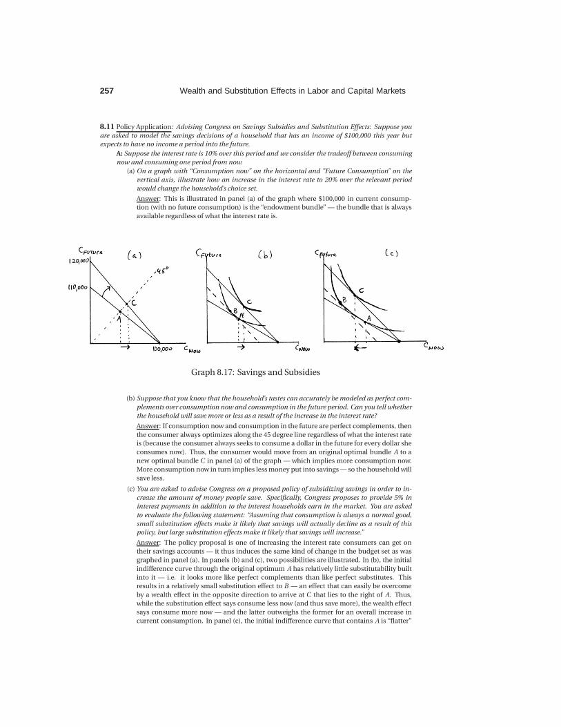
257 Wealth and Substitution Effects in Labor and Capital Markets
8.11 Policy Application: Advising Congress on Savings Subsidies and Substitution Effects: Suppose you
are asked to model the savings decisions of a household that has an income of $100,000 this year but
expects to have no income a period into the future.
A: Suppose the interest rate is 10% over this period and we consider the tradeoff between consuming
now and consuming one period from now.
(a) On a graph with “Consumption now” on the horizontal and ”Future Consumption” on the
vertical axis, illustrate how an increase in the interest rate to 20% over the relevant period
would change the household’s choice set.
Answer: This is illustrated in panel (a) of the graph where $100,000 in current consump-
tion (with no future consumption) is the “endowment bundle” — the bundle that is always
available regardless of what the interest rate is.
Graph 8.17: Savings and Subsidies
(b) Suppose that you know that the household’s tastes can accurately be modeled as perfect com-
plements over consumption now and consumption in the future period. Can you tell whether
the household will save more or less as a result of the increase in the interest rate?
Answer: If consumption now and consumption in the future are perfect complements, then
the consumer always optimizes along the 45 degree line regardless of what the interest rate
is (because the consumer always seeks to consume a dollar in the future for every dollar she
consumes now). Thus, the consumer would move from an original optimal bundle A to a
new optimal bundle C in panel (a) of the graph — which implies more consumption now.
More consumption now in turn implies less money put into savings — so the household will
save less.
(c) You are asked to advise Congress on a proposed policy of subsidizing savings in order to in-
crease the amount of money people save. Specifically, Congress proposes to provide 5% in
interest payments in addition to the interest households earn in the market. You are asked
to evaluate the following statement: “Assuming that consumption is always a normal good,
small substitution effects make it likely that savings will actually decline as a result of this
policy, but large substitution effects make it likely that savings will increase.”
Answer: The policy proposal is one of increasing the interest rate consumers can get on
their savings accounts — it thus induces the same kind of change in the budget set as was
graphed in panel (a). In panels (b) and (c), two possibilities are illustrated. In (b), the initial
indifference curve through the original optimum A has relatively little substitutability built
into it — i.e. it looks more like perfect complements than like perfect substitutes. This
results in a relatively small substitution effect to B — an effect that can easily be overcome
by a wealth effect in the opposite direction to arrive at C that lies to the right of A. Thus,
while the substitution effect says consume less now (and thus save more), the wealth effect
says consume more now — and the latter outweighs the former for an overall increase in
current consumption. In panel (c), the initial indifference curve that contains A is “flatter”
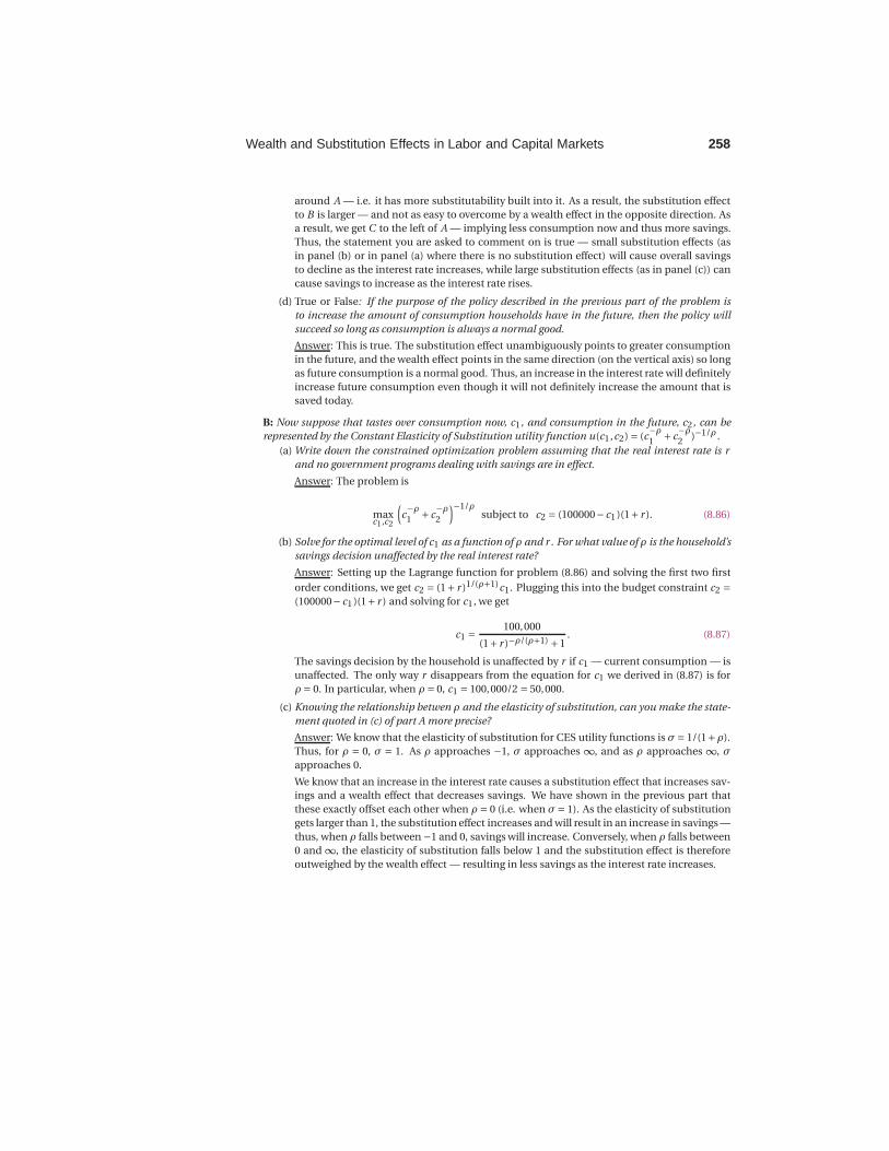
Wealth and Substitution Effects in Labor and Capital Markets 258
around A — i.e. it has more substitutability built into it. As a result, the substitution effect
to B is larger — and not as easy to overcome by a wealth effect in the opposite direction. As
a result, we get C to the left of A — implying less consumption now and thus more savings.
Thus, the statement you are asked to comment on is true — small substitution effects (as
in panel (b) or in panel (a) where there is no substitution effect) will cause overall savings
to decline as the interest rate increases, while large substitution effects (as in panel (c)) can
cause savings to increase as the interest rate rises.
(d) True or False: If the purpose of the policy described in the previous part of the problem is
to increase the amount of consumption households have in the future, then the policy will
succeed so long as consumption is always a normal good.
Answer: This is true. The substitution effect unambiguously points to greater consumption
in the future, and the wealth effect points in the same direction (on the vertical axis) so long
as future consumption is a normal good. Thus, an increase in the interest rate will definitely
increase future consumption even though it will not definitely increase the amount that is
saved today.
B: Now suppose that tastes over consumption now, c1, and consumption in the future, c2, can be
represented by the Constant Elasticity of Substitution utility function u(c1,c2) = (c−ρ1
+c−ρ2
)−1/ρ .
(a) Write down the constrained optimization problem assuming that the real interest rate is r
and no government programs dealing with savings are in effect.
Answer: The problem is
maxc1,c2
(c−ρ1 +c
−ρ2
)−1/ρsubject to c2 = (100000−c1 )(1+ r ). (8.86)
(b) Solve for the optimal level of c1 as a function of ρ and r . For what value ofρ is the household’s
savings decision unaffected by the real interest rate?
Answer: Setting up the Lagrange function for problem (8.86) and solving the first two first
order conditions, we get c2 = (1+ r )1/(ρ+1)c1. Plugging this into the budget constraint c2 =(100000−c1 )(1+ r ) and solving for c1, we get
c1 =100,000
(1+ r )−ρ/(ρ+1) +1. (8.87)
The savings decision by the household is unaffected by r if c1 — current consumption — is
unaffected. The only way r disappears from the equation for c1 we derived in (8.87) is for
ρ = 0. In particular, when ρ = 0, c1 = 100,000/2 = 50,000.
(c) Knowing the relationship betwen ρ and the elasticity of substitution, can you make the state-
ment quoted in (c) of part A more precise?
Answer: We know that the elasticity of substitution for CES utility functions is σ= 1/(1+ρ).
Thus, for ρ = 0, σ = 1. As ρ approaches −1, σ approaches ∞, and as ρ approaches ∞, σ
approaches 0.
We know that an increase in the interest rate causes a substitution effect that increases sav-
ings and a wealth effect that decreases savings. We have shown in the previous part that
these exactly offset each other when ρ = 0 (i.e. when σ= 1). As the elasticity of substitution
gets larger than 1, the substitution effect increases and will result in an increase in savings —
thus, when ρ falls between −1 and 0, savings will increase. Conversely, when ρ falls between
0 and ∞, the elasticity of substitution falls below 1 and the substitution effect is therefore
outweighed by the wealth effect — resulting in less savings as the interest rate increases.