The first step in energy management

Andrew Ibbotson

Joe Flanagan

Energy Survey Workshop

What is an energy survey?

For a site, dept, or process

• Establishes the energy cost and consumption

• Is a technical investigation of the energy flows

• Aims to identify cost effective energy savings

• Examines both the technical and ‘soft’

management issues.

Why carry out a survey?

Identify savings

Establish the viability of an energy management programme

Establish a ‘baseline’

Identify where Energy is Used and Develop an Action Plan

Senior Management Commitment

Produce Reports to Monitor Energy Use Against Output

Review Performance and Action Plan

Implement Energy Saving Measures

Measure Energy Consumption and Production

Develop Targets

Survey

The Energy Management Process

DIY or Consultant? Consultant

Expertise

Fresh pair of eyes

Should not be afraid to poke into any corner

Opinions may carry more weight

Job will be completed

DIY

No cost

No learning curve

Projects should be viable

Choosing a Consultant

Salesman or consultant?

Ensure he/she is experienced in your process

Don’t be afraid to take up references

Cost - day rate of fixed price

1. Define the scope

2. Establish energy balances

3. Identify priority areas

4. Identify energy saving projects Low cost (control, housekeeping, awareness)

Medium cost (revenue expenditure <1 year payback)

High cost (capital expenditure <2-3 year payback)

5. Reporting

The Survey Process

Depends upon

complexity of the site and scope

Level of detail available (esp. sub-meters)

Size and energy intensity

Rule of thumb

Up to €200,000 – 6 mandays

Up to €1,000,000 – 10-15 mandays

How much effort is required?

Electricity, gas, oil, solid fuel etc

?Water, effluent, industrial gases

In general further detailed study will be required for medium and high cost opportunities

Scope

Last 12 months bills

Sub-meter readings

Principal energy users

Production and climatic data

1st Law of Thermodynamics – energy can neither be created or destroyed

Energy Balances and Data Analysis

Maximum Demand charges (kVA, kW)

Capacity charges (kVA, kW)

Day and night rates

Power factor

Electricity Bills

kWhkWh

kVAhkVAhkVArhkVArh

φφPF = kWh/kVAh

= cos φ

PF = kWh/kVAh

= cos φ

From the electricity bill

kWh = 17,400

kVArh = 8,700

What is the power factor?

From the electricity bill

kWh = 17,400

kVArh = 8,700

What is the power factor?

Power Factor

Power factor

tan φ = 8,700/17,400

= 0.5

φ = 26.5º

cos 26.5 = 0.89

PF improved by adding capacitors

Worthy of further investigation below 0.85-0.90

Date 00:30 01:00 01:30 02:00 02:30 03:00 03:30 04:00 04:30 05:00 05:30

01-Jan-02 Tue 144 148 146 146 148 146 148 148 148 152 146

02-Jan-02 Wed 586 576 570 558 572 558 560 568 562 564 560

03-Jan-02 Thu 570 580 550 568 564 568 556 576 574 546 568

04-Jan-02 Fri 544 570 572 566 566 574 568 562 566 582 568

05-Jan-02 Sat 544 560 516 506 452 408 400 412 416 408 374

06-Jan-02 Sun 494 512 504 504 514 506 516 524 526 510 528

07-Jan-02 Mon 594 574 570 562 554 542 534 544 538 550 518

08-Jan-02 Tue 584 574 570 564 566 566 562 564 572 566 568

09-Jan-02 Wed 576 550 556 568 570 560 568 566 552 560 568

10-Jan-02 Thu 568 556 564 556 548 526 538 544 550 536 524

11-Jan-02 Fri 576 568 578 568 572 566 564 570 538 564 576

12-Jan-02 Sat 458 446 422 406 360 294 290 272 228 190 174

13-Jan-02 Sun 502 502 492 486 472 506 508 512 508 478 508

14-Jan-02 Mon 590 572 566 564 552 544 548 572 584 536 534

15-Jan-02 Tue 602 582 568 580 562 562 560 572 590 580 572

16-Jan-02 Wed 562 560 562 524 544 546 558 542 540 538 544

17-Jan-02 Thu 570 566 572 546 562 542 554 554 522 542 564

18-Jan-02 Fri 586 588 572 566 576 568 570 574 556 580 576

19-Jan-02 Sat 344 292 282 230 196 194 194 194 198 204 204

20-Jan-02 Sun 496 504 506 502 504 506 492 516 518 508 526

21-Jan-02 Mon 586 574 524 560 560 560 564 556 560 560 540

22-Jan-02 Tue 582 572 576 544 546 566 566 572 558 544 562

23-Jan-02 Wed 564 572 536 552 552 550 544 558 532 564 566

24-Jan-02 Thu 566 570 564 538 544 546 522 566 560 562 566

25-Jan-02 Fri 570 572 572 550 562 556 542 532 572 560 570

26-Jan-02 Sat 408 398 354 336 288 234 226 210 206 210 210

27-Jan-02 Sun 512 510 490 502 468 442 444 452 454 446 458

Date 00:30 01:00 01:30 02:00 02:30 03:00 03:30 04:00 04:30 05:00 05:30

01-Jan-02 Tue 144 148 146 146 148 146 148 148 148 152 146

02-Jan-02 Wed 586 576 570 558 572 558 560 568 562 564 560

03-Jan-02 Thu 570 580 550 568 564 568 556 576 574 546 568

04-Jan-02 Fri 544 570 572 566 566 574 568 562 566 582 568

05-Jan-02 Sat 544 560 516 506 452 408 400 412 416 408 374

06-Jan-02 Sun 494 512 504 504 514 506 516 524 526 510 528

07-Jan-02 Mon 594 574 570 562 554 542 534 544 538 550 518

08-Jan-02 Tue 584 574 570 564 566 566 562 564 572 566 568

09-Jan-02 Wed 576 550 556 568 570 560 568 566 552 560 568

10-Jan-02 Thu 568 556 564 556 548 526 538 544 550 536 524

11-Jan-02 Fri 576 568 578 568 572 566 564 570 538 564 576

12-Jan-02 Sat 458 446 422 406 360 294 290 272 228 190 174

13-Jan-02 Sun 502 502 492 486 472 506 508 512 508 478 508

14-Jan-02 Mon 590 572 566 564 552 544 548 572 584 536 534

15-Jan-02 Tue 602 582 568 580 562 562 560 572 590 580 572

16-Jan-02 Wed 562 560 562 524 544 546 558 542 540 538 544

17-Jan-02 Thu 570 566 572 546 562 542 554 554 522 542 564

18-Jan-02 Fri 586 588 572 566 576 568 570 574 556 580 576

19-Jan-02 Sat 344 292 282 230 196 194 194 194 198 204 204

20-Jan-02 Sun 496 504 506 502 504 506 492 516 518 508 526

21-Jan-02 Mon 586 574 524 560 560 560 564 556 560 560 540

22-Jan-02 Tue 582 572 576 544 546 566 566 572 558 544 562

23-Jan-02 Wed 564 572 536 552 552 550 544 558 532 564 566

24-Jan-02 Thu 566 570 564 538 544 546 522 566 560 562 566

25-Jan-02 Fri 570 572 572 550 562 556 542 532 572 560 570

26-Jan-02 Sat 408 398 354 336 288 234 226 210 206 210 210

27-Jan-02 Sun 512 510 490 502 468 442 444 452 454 446 458

Average Electricity Half Hourly Data Lock Street (Year to 30/9/02)

0

100

200

300

400

500

600

700

00:0

001

:00

02:0

003

:00

04:0

005

:00

06:0

007

:00

08:0

009

:00

10:0

011

:00

12:0

013

:00

14:0

015

:00

16:0

017

:00

18:0

019

:00

20:0

021

:00

22:0

023

:00

kWh

per

1/2

ho

ur

Monday

Tuesday

Wednesday

Thursday

Friday

Saturday

Sunday

Gas Bills

• More frequently estimated (in the UK)

• Errors more prevalent

• Very rarely obtain ½ hourly demand

• Can obtain some useful energy management information

0

50,000

100,000

150,000

200,000

250,000

300,000

350,000

400,000

450,000

500,000

Jan-99 Feb-99 Mar-99 Apr-99 May-99 Jun-99 Jul-99 Aug-99 Sep-99 Oct-99 Nov-99 Dec-99

kW

h/m

on

th

‘Base’ or process gas load

‘Base’ or process gas load

Electrical Balance

• Sub-meters help – but rarely provide all the required information

• Need to list major electrical consumers (pumps, fans, compressors, chillers, lighting, process heating etc)

• Need rating and running hours

Estimating Electricity

Load Design kW

Actual kW

Load factor

Hours per year

kWh

Grinder 150 120 0.7 4000 336,000

Pump 55 55 1 6000 330,000

Compressor 150 140 0.5 6000 420,000

Lights 25 25 1 3000 75,000

Total 1,161,000

Estimating Electricity

Load Design kW

Actual kW

Load factor

Hours per year

kWh

Grinder 150 120 0.7 4000 336,000

Pump 55 55 1 6000 330,000

Compressor 150 140 0.5 6000 420,000

Lights 25 25 1 3000 75,000

Total 1,161,000

Design kW = rating on equipment

e.g. plate rating of a motor; wattage of a bulb

Estimating Electricity

Load Design kW

Actual kW

Load factor

Hours per year

kWh

Grinder 150 120 0.7 4000 336,000

Pump 55 55 1 6000 330,000

Compressor 150 140 0.5 6000 420,000

Lights 25 25 1 3000 75,000

Total 1,161,000

Actual kW = best estimate of actual power

e.g. based on ammeter reading or design data

kW = √3*V * I * PFkW = √3*V * I * PF

Estimating Electricity

Load Design kW

Actual kW

Load factor

Hours per year

kWh

Grinder 150 120 0.7 4000 336,000

Pump 55 55 1 6000 330,000

Compressor 150 140 0.5 6000 420,000

Lights 25 25 1 3000 75,000

Total 1,161,000

Load factor allows for variable load

e.g. air compressor on load / off load

Estimating Electricity

Load Design kW

Actual kW

Load factor

Hours per year

kWh

Grinder 150 120 0.7 4000 336,000

Pump 55 55 1 6000 330,000

Compressor 150 140 0.5 6000 420,000

Lights 25 25 1 3000 75,000

Total 1,161,000

Total should = metered total

either for whole site or for a sub-meter

Estimating Electricity

• High accuracy is time consuming

• ±10% is very good

• Portable data logger useful for large users

• Don’t underestimate the large number of small users e.g. conveyors, fans, pumps

Electricity Balance

Furnace Cooling Fans14%

Lighting17%

Compressors13%K Line EP

11%

Furnace Water Pumps7%

Bath Heating6%

Bath bottom cooling fans4%

Lehr Fans 3%

Batch Plant2%

Lehr Heating2%

Other10%

Fin Fan Coolers11%

Fuel Balances

• Process vs. space heating from a year of monthly or weekly data

• Difficult to estimate the distribution among process users if there is no metering

• Most gas process plant will operate well below MCR – manufacturers specification

• No portable gas metering

Could CHP be feasible?

• Power demand >500 kW

• Coincident heat (steam or hot water) demand?

• Heat to power 3:1

• High operating hours > 2 shift 5d/week

Benchmarking

• Comparison to a published benchmark often seen as method for estimating savings

• Treat with caution

> ‘best practice’ often refers to ‘state of the art’

> Utilisation has a large influence

• Generally confirms what you already know

• Greatest validity for ‘basic’ industry – metals, ceramics, glass etc..

• Lots of information at www.actionenergy.org.uk

Boilers & Steam Systems

Scope

Basic Combustion Process

Natural gas

8N2 + CH4 + 2O2 CO2 + 2H2O + 8N2

Plus the release of ~10 kWh/m3 of CH4

10 volumes of air required for 1 volume of methane

Heat Recovery Process

Burner Furnace Tube - radiation

Gas Passes - convection

Boiler Losses

Exhaust(~20% on gas, ~16% on oil)

Blowdown(<5%)

Convection & Radiation

(1% to 1.5% @ max continuous

rating (mcr))

Air & Fuel

Convection proportional to TRadiation proportional to T4

Combustion Losses

• heat loss in flue gases

• Latent heat of water vapour in flue gases

• incomplete carbon combustion

• ‘Excess’ air must be kept to a minimum

• Generally at least 10% excess is required to ensure good combustion

• Combustion losses depend upon volume and temperature of flue gases

Excess Air

• measured by inference from O2 in exhaust or level of CO2 in exhaust

• Portable instrument (measures O2, temp and CO

• Permanent zirconia probe in stack linked to air/gas valves (oxygen trim)

Best Boiler Efficiency

• optimised fuel / air ratio well insulated (shiny surface)

• clean burner nozzles

• clean boiler surfaces

• minimum steam pressure / temperature

• reasonable load (~80%)

• optimised TDS controlling blowdown

Combustion

• 1% efficiency increase, 79% to 80% savers 1- 0.8 = 1.25% fuel

> reduction of 02 by ~2%

> reduction of exhaust temperature by ~20ºC

• oxygen trim control; 1% to 1.5% on well adjusted boiler

• Air preheat (duct from air compressors or boilerhouse) saving 0.5% to 1%

Blowdown

• maintaining recommended TDS levels ensures clean heat transfer surfaces

• operating low TDS waste energy, water, chemicals and increases effluent costs

• heat recovery (for large boilers payback 2-3 years)

Other

• check optimum load on boilers

• rank multiple boilers to operate the group with minimum loss

• Shutdown Loss Minimisation

> gas side isolation with dampers

> water/steam side isolation with crown valve

Heat Recovery

• economiser (to feedwater)

• recuperator (to wash water)

Insulation

• check existing quality

• insulate all hot pipework, flanges (1m pipe), valve bodies (5m pipe)

• hotwell cover and insulation

Key Points for the Boiler House

Check

• Boiler efficiency

• Blowdown procedure

• Condensate return

• insulation

The Nature of Steam

Item Heat Content

KJ/kg %

Latent at 7 bar g 2050 74

Flash at Atmospheric from 7 bar g 300 11

Condensate at Atmospheric 420 15

Total 2770 100

Breakdown of heat content of 7 bar g saturated steam

System Standing Losses

Fixed loss from:

• Pipework

• Valves

• Fittings etc.

Losses range from 2% to 5%

System Variable Losses

Flash and % losses with steam at

condensate ? bar g & cond. at 0 bar g

return 7 5 3 0

Total loss 26 24 22 15

50% cond. return 19 17 15 7

Management Control

• Automatic isolation systems

• Pressure reduction

• Energy management:

> Metering

> Data analysis

> Action

Fixed Losses

• Insulation

• air ingress

• steam leaks

Pipework

• Size:

> cost trade-off

• Installation:

> air removal

> condensate drainage

> weather sealing

> group users

Pressure Reduction

• More efficient

• Saves fuel

• Cost incurred for:

> pressure reduction sets

> larger heat exchangers

> larger traps

• Consider life cycle costs

Steam Leaks

1000800

Examples:Steam Leak = 7.5mm diameterSteam Pressure (barg) ( or pressure difference between steam and condensate) = 6 barSteam Loss = 100 kg/h

600

400

200

1008060

40

20

1086

43

2 3 45 7 10 14

12.5 mm10 mm

7.5 mm

5 mm

3 mm

Steam Trapping & Air Venting

• Steam trapping> function> testing> group trapping> sizing traps

• Air venting

• Scale and dirt removal

Condensate Recovery

Saves costs for:

• Water

• Treatment chemicals

• Fuel

• Effluent

Produces rapid payback

Flash Steam Recovery

By:• Indirect method• Direct method

Potential sinks:• BFW• Wash water• Process fluid• Space heating

Key Points for Steam Systems

• Pipe insulation

• Leaks

• Isolation of redundant plant/off line plant

• Steam traps

• Condensate return

Lighting

Lighting

• Overview of main industrial lighting types

• Their efficiency

• Common savings

Lighting

• Typically 10-50% of electricity use

• Good lighting is critical to all manufacturing operations

• Survey is relatively easy to carry out

Estimate of Load

• Rating of lamp

• Number

• Operating hours

• Add 10% for control gear

Common Industrial Lighting Types

• Fluorescent> Offices, general manufacturing

> Good colour rendering

> Instant instantaneous on and off

• Metal Halide (HPI, MBI)> Good colour rendering

• High Pressure Sodium (SON)> Poor colour rendering

• Low Pressure Sodium (SOX)> Very poor colour (orange yellow)

> Very efficient

Comparison of Lamp Types

Lamp Type Lumens/watt Standard Life hrs (50% survival)

GLS 12 1,000

CFL 70 8,000

T8 70-100 6,000-15,000

T12 70 5,000-10,000

Metal halide 60-80 6,000-13,000

SON 108 15,000-30,000

SOX 138 12,000-23,000

Induction 70 60,000 (80%)

Typical Illuminance Levels

Lux Activity

50 Cable tunnels, walkways

100 Corridors, bulk stores

150 Loading bays. Plant rooms

300 Offices (300/500), assembly

500 Engine assembly, painting spraying

750 Ceramic decoration, meat inspection

1000 Electronic assembly, toolrooms

1500 Precision assembly

Savings with Fluorescents

• Change T12 for T8

• Control (PIR, zoning, daylight)

• New systems> High frequency ballasts

> High efficiency reflectors/diffusers

> Payback 2-4 years

Length T8 (ø26mm) T12 (ø38mm)

600mm 2’ 18W 20W

1200mm 4’ 36W 40W

1500mm 5’ 58W 65W

1800mm 6’ 70W 75/85W

2400mm 8’ 100W 125W

Savings with Metal Halides

• Convert to SON (beware of colour issues)

• Payback ~1 year if replace 400W MBF to 250W SON (8760h/y). Cost of SON €100

• Convert to fluorescent if switching off is possible

Top Tips for Lighting

• Lux measurement is worthwhile

• Switch off

• Need high lighting hours (2 shift) to justify replacement

• Plenty of suppliers will carry out free surveys

Compressed Air

Compressed Air

• Background to Compressed Air

• Reducing loads and pressure

• Improving distribution

• Improving generation

Compressed Air

• very expensive form of energy

> typically costs 1€/kWh

• often used unnecessarily or inappropriately

> Cooling, cleaning etc

• similar philosophy to steam / refrigeration

> minimise loads and pressures

> minimise distribution system losses

> maximise generation efficiency

Potential Savings

• Compressed air can account for up to 20% electricity use.

• Enviros study identified minimum potential savings of 27%

> generation (7%)

> distribution (11%)

> end usage (3%)

> new technology (6%)

Compressed Air System Components

What to look out for - use

• Leaks

• Main uses of air such as tools, painting, instrumentation or process

• Misuses such as open ended lances, full pressure blow guns, product ejection and vacuum venturis

• End of line pressure

• Ring or spur mains?

Check Each Load

• why is air being used

> a key requirement or ‘habit’?

• can a load be eliminated or reduced

> replace pneumatic valves with electric

> ‘amplifier’ nozzles

• pressure and air quality requirements

> is it as low as possible

> how does it compare with other loads

Three main issues:Three main issues:• pressure dropspressure drops• waterwater• leaksleaks

Distribution

The Distribution System

• examine the pressure drop across the system (velocity 6-9 m/s)

• pipework is rarely upgraded when system extended

• small bore pipe, elbows and short bends increase pressure drop

• internal corrosion increases friction losses

• A 1 bar pressure drop increases energy cost by 10%

Distribution Lines – The Effect of Water

• Problems with water

> Causes corrosion

> Product quality

> Increases pressure drops

• Is drying adequate? Additional automatic drain points

Leakage Losses

• typically 25 - 50% of full load usage!

• regular maintenance required to identify and repair leaks especially where flexible connections are used

• identify and tag leaks at the weekend when production areas are quiet

Leak reduction

Leakage Losses

Hole diameter Leakage at 7 bar/100 psi

Equiv. Power

mm Inches l/s scfm kW

0.4 1/64 0.2 0.4 0.1

1.6 1/16 3.1 6.5 1.0

3.0 1/8 11.0 23.2 3.5

Some Ways of Reducing Losses

• Isolate air supplies outside working hours> to the machines

> Interlock air supply with machinery

> to areas of the factory with different working hours

• Use the lowest possible operating pressure> reduce pressure locally if possible

• If some consumers use low pressure air install a separate system

75%75%Energy CostEnergy Cost

10%10%MaintenanceMaintenance

15%15%CapitalCapital

Life Cycle Costs of Compressor

• Type, make, capacity, hours run and control of each compressor

• Type make and configuration of treatment package

• Room ventilation, inlets in or outside?

• Is waste heat recovered?

• What is the generation pressure?

• Is there a group controller?

• What is the estimated demand?

• Are the feeding mains OK are there any other bottlenecks?

• Do they have electronic zero loss condensate traps?

What to look out for in the Compressor Room

Filtration

• Filters cause pressure drops.

> To save energy meet the minimum requirement

> Undersizing raises pressure drop

> Every 25mbar pressure drop increases compressor power consumption by 2%

Drying

• Ambient air at 15oC contains about 12.5g water per cubic metre

• Most condenses in the aftercooler> An after cooler might remove 68% of the water in the air

if cooled to 35oC

• Further drying is usually necessary> Deliquescent - energy efficient, cheap

> Refrigerated - popular, 3-5% energy cost (dew point 3ºC)

> Desiccant – air regenerated can consume 15-20% of air produced (dew point -60ºC)

Guidelines for Drying

• Generally design to dry air to 6ºC below ambient temperature

• Don’t run pipework outside if possible

• Only dry as much air as is necessary (i.e.

have a separate wet and dry system)

Configuration Capacity Nm3/h Specific PowerkWh/Nm 3

Control

Lubricated Piston2-25

25-250250-1,000

14.211.810.0

Good with step unloading and lowoff load power

Oil Free Piston2-25

25-250250-1,000

15.313.011.2

Good with step unloading and lowoff load power

Lubricated Screw/Vane2-25

25-250250-1,000

14.212.411.2

High power on part load

Oil Free Screw25-250

250-1,0001,000-2,000

11.910.610.6

Two step with good part load power

Centrifugal250-1,000

1,000-2,000Above 2,000

12.410.610.0

Good over modulation range

Compressor Efficiencies

Reciprocating Compressors

• Single or multi stage

• Idling losses normally around 25% of full load current

• Relatively efficient on part load

• Valve deterioration reduces efficiency

• Noisy

• High maintenance

Rotary Screw Compressors

• Normally provide cleaner air

• Most popular unit

• Packaged units available with integral heat recovery

• Very efficient if run with variable speed control

• Unloaded power greater than reciprocating machines

Centrifugal Compressors

• High capacity base load machines

• Large machines have very good efficiency on full load

• Part load operation achieved by inlet throttling modulation

• Modulation should only be used around full load conditions, very poor efficiency at low loads

Rotary Sliding Vane

• Normally used for less demanding duties

• Generally low capital cost machines

• Used for single shift operations

• No integral heat recovery

• Part load operation very inefficient

Control - General Rules

• On/off control (where possible) is better than variable speed, which is better than modulating control

• Modern control systems can select the optimum combination of compressors

• For multiple compressors check hours run and loaded meters

Modulating and Variable Speed Control

100%

50% 100%

Power

Output

Variable Speed

Modulating

Heat Recovery

• Process

> Drying

> Heating

• Building Services

> Space Heating

> Water Heating

• Compressed Air Treatment

> Dryers

• Boiler Pre-heating

> Feed Water

> Combustion Air

Into air or water for:

Heat Recovery Example

• A 20kW compressor would satisfy the combustion air requirements of a 1 MW boiler

• For each 20oC rise in combustion air temperature there is an approximate 1% rise in boiler efficiency.

• If this air is at 60oC, an efficiency increase of 3% may result.

2422884000090002501500

1934967100075002001200

154245350005600160900

105353650003700110600

5263182000160055300

20767200081022120

1249440004501580

Gas equivalent£

Heat availableWarm air flowL/s

Motor PowerKW

Capacity cfm

Heat available from compressors at full load

Heat Recovery Potential

Intake Air Temperature

For every 4For every 4C that the intake air C that the intake air temperature falls: temperature falls:

The energy required for The energy required for compression falls by 1%compression falls by 1%

Intake Air Temperature - Example

• A compressor draws air from a plant room that is typically at 25oC, and consumes 75kW

• The average UK/Ireland outside air temperature is 10oC

• Taking the air from outside means that the average temperature is 15oC lower

• Saving 3.75%, 2.8kW, £1000/yr

Summary

• compressed air is very expensive

> often equivalent to >50p/kWh

• only use when really necessary

• minimise system pressure

• minimise leaks

> simplify distribution

> isolate unused sections

• optimise generation efficiency

Top Tips

• Check compressor instrumentation (hrs run, on-load etc.)

• Simple ‘rotameters’ for (temporary) flow measurement are very cheap

• Install automatic drain traps

• Look carefully what happens at meal breaks, shift changes and weekends

Energy Management

Level

Energy Policy

Organising

Motivation

Information

Systems

Marketing

Investment

4 Energy policy, action plan and regular review have commitment of top management as part of an environmental strategy

Energy management fully integrated into management structure. Clear delegation of responsibility for energy consumption.

Formal and informal channels of communication regularly exploited by energy manager and energy staff at all levels.

Comprehensive system sets targets, monitors consumption, identifies faults, quantifies savings and provides budget tracking.

Marketing the value of energy efficiency and the performance of energy management both within the organisation and outside it.

Positive discrimination in favour of ‘green’ schemes with detailed investment appraisal of all new-build and refurbishment opportunities.

3 Formal energy policy, but no active commitment from top management.

Energy manager accountable to energy committee representing all users, chaired by a member of the managing board.

Energy committee used as main channel together with direct contact with major users.

M&T reports for individual premises based on sub-metering, but savings not reported effectively to users.

Programme of staff awareness and regular publicity campaigns.

Same pay back criteria employed as for all other investment.

2 Un-adopted energy policy set by energy manager or senior departmental manager.

Energy manager in post, reporting to ad-hoc committee, but line management and authority are unclear.

Contact with major users through ad-hoc committee chaired by senior departmental manager.

Monitoring and targeting reports based on supply meter data. Energy unit has ad-hoc involvement in budget setting.

Some ad-hoc staff awareness training.

Investment using short-term payback criteria only.

1 An unwritten set of guidelines

Energy management is the part-time responsibility of someone with limited authority or influence

Informal contacts between engineer and a few users.

Cost reporting based on invoice data. Engineer compiles reports for internal use within technical department.

Informal contacts used to promote energy efficiency.

Only low cost measures taken.

0 No explicit policy No energy management or any formal delegation of responsibility for energy consumption

No contact with users.

No information system. No accounting for energy consumption.

No promotion of energy efficiency.

No investment in increasing energy efficiency in premises.

Expectations have been raised

The two outside columns are significantly higher

U-shaped3

Is this balance a symptom or orderly progress or stagnation

Balanced score of less than 3 on all columns

Low Balanced

2

Excellent performance; the challenge is to maintain this high standard

Score 3 or more on all columns

High Balanced

1

DiagnosisDescriptionShape

The more imbalance the harder it is to perform well

Two or more columns are 2 points above or below average

Unbalanced7

Effort in this area could be wasted by lack of progress elsewhere

A single column is significant higher than the rest

Peak6

Underachievement in this column may well hold back success elsewhere

A single column is significantly lower than the rest

Trough5

Achievement in the centre is likely to be wasted

The two outside columns are significantly lower

N-shaped4

DiagnosisDescriptionShape

Refrigeration

General comments

• Refrigeration systems are often complex

• Maintenance often sub-contracted

• Poor energy efficiency not obvious

• Savings potential is good ~20%

The Refrigeration Process (1)

Condenser

Evaporator

Substance Being Cooled

Ambient Cooling Stream

Low P

High P Compressor

High pressure vapour

High pressure liquid

Expansion valve

Low pressure liquid/vapour

Low pressure vapour

Refrigerants - A Few Examples

• Ammonia R717

• CFCs R11, R12, R502

• HCFC R22

• Pure HFCs R134a, R32

• HCFC blends R403B, R408A

• HFC blends R404A, R507

• Hydrocarbons R290

System Efficiency

Coefficient of Performance (COP) = useful cooling/system power

Theoretical efficiency (Carnot efficiency)= Te/(Tc – Te) (T is degK)

Useful approximation COP=0.6Te/(Tc – Te)

Chillers often specified in tons (US) 1 ton = 200 BTU/min (3.52kW)

Measurement of Tc & Te

• Often chillers only equipped with pressure gauges

• Pressure can be converted temp. if refrigerant is known

Typical Compressor COPs

COP

Air Conditioning 15°C 5

Chilling 3°C 4

Freezing -30°C 2

Calculation of COP

• Need to know

• Compressor power

• Flow/return temps of primary/secondary refrigerant

• Flow rate of primary/secondary refrigerant

• Thermodynamic properties/specific heat of primary/secondary refrigerant

• Only possible on large systems

Improving COP

• From Carnot = Te/(Tc – Te) theoretical efficiency increases as:

• Tc – Te approach 0

• Te increases for the same temperature lift (Tc – Te)

Increasing Te

• Efficient heat transfer in evaporator

> Clean heat exchange surfaces (e.g. ice on evaporator)

• Avoid overcooling of product

> e.g. product stored at -20ºC, but freezer cools to -30ºC

• Temperature set point unnecessarily; low ΔT between refrigerant and process liquid <5ºC

> Two stage cooling

• Increase Te 1ºC increases efficiency by ~3%

Condensers

• Water cooled shell and tube (with CT)

> Water approach temp 5ºC

> Water temp rise ~ 5ºC

> Condensing temp 15 ºC greater than wet bulb

• Air cooled> Condensing temp 15 ºC greater than air

• Evaporative condensers

> Similar to shell and tube

• Decrease Tc 1ºC increases efficiency by ~3%

Compressor Performance

% of full load COP

100

50

0% 100%% of full duty

Reciprocating

Centrifugaland screw

Modular Design, 3 water chillers

Case Study (a) poor part load control of 3 modular water chillers

Load % Power kW

Compressor 1 33 902 33 903 33 90

Chilled water pumps 1 100 252 100 253 100 25

Condenser pumps 1 100 202 100 203 100 20

Total Power Absorbed - 405

Case Study (b) good control

Load % Power kW

Compressor 1 100 1502 0 03 0 0

Chilled water pumps 1 100 252 0 03 0 0

Condenser pumps 1 100 202 0 03 0 0

Total Power Absorbed - 195

What can be easily assessed?

• If possible calculate COP

• Minimise cooling loads

> Free cooling in HVAC systems

> Two stage

> Cold store housekeeping

• Check ΔTs

> Condition of heat exchangers

Using Variable Speed Drives

and Efficient Motors

Content

• Background to Motors and Drives

• Using High Efficiency Motors

• Using soft starts for better control

• Using voltage controllers for partly loaded

motors

• Using variable speed drives

Motor and Drives

• constitute over half of industrial electrical demand

• overall saving potential - 10% across Industrial & Commercial sectors

• A motor will consume its capital cost in just a month of continuous operation. SoThe capital investment is insignificant compared to running costs.

Motor Operation Costs

0

500

1000

1500

2000

2500

3000

3500

4000

4500

5000

0 100 200 300 400 500 600 700 800 900Hours in use

£

132kW motor

132kW running cost

22kW motor

22kW running costs

132kW motor, cost £3600, efficiency 93%22kW motor, cost £660, efficiency 90%Electricity cost 4p/kWh, both motors fully loaded

Typical Motor Efficiency (simplified)

0

25

50

75

100

0 25 50 75 100 125% load

% e

ffic

ien

cy

Motor Rating (kW)

Mo

tor

Eff

icie

ncy

%

Nominal Motor Efficiency v. Rating

% E

ffic

ienc

y

kW1.1 90

The European EfficiencyLabeling Scheme

iron loss

friction and windage

I2R (copper)

lossstray loss

Total Loss

0 40 80 120

12

9

6

3

0

Load (%)

FullLoadPowerLoss (%)

High Efficiency Motors

• reduced Iron (Steel) Losses

• reduced copper Losses

• stray losses minimised

• more efficient motor generates less heat

High Efficiency Versus Standard Motors Payback Period

New Motor - 7.5 kW

Hours of Electricity Additional PaybackUsage p.a. Cost Savings Costs Years £ p.a. £

2000 36 83 2.3

4000 72 83 1.2

6000 108 83 0.8

At 4p/kWh for electricity, the incremental cost payback occurs after about

5000 hours.

High Efficiency Motors - Conclusions

• most suitable for highly loaded motors

• justified on new or replacement motors

> rewinds introduce extra losses – buy HEM instead of rewinding

• on 4,000 hrs or more operation, marginal payback just over a year

Switch it off!

• don’t leave motors running needlessly

• fit automatic controls to avoid motors being left on

> e.g. timers or load sensors on conveyors

• look for fixed loads

> e.g. tank mixers – why not switch motor off for 1 minute every 5 with a saving of 20%

Soft start equipment

• can enable switch off strategies to work

• gives a more controlled motor start

> by ramping up motor voltage

> replaces DOL or star-delta starters

• reduces power surge

• reduces mechanical wear on motor, drive and connected equipment

• makes it possible to stop and start motors more frequently

Motor Voltage Controllers

• improve efficiency at loads below 50%

> regulate the voltage at the motor terminals

> iron losses are reduced

> efficiency and power factor are improved

• suitable for variable load motors that operate under 50% load for long periods

• do not use on highly loaded motors

> reduce efficiency at high load!

Variable Speed Drives

• excellent “new” technology to help reduce

electricity consumption

• for pumps / fans savings can be dramatic

> cubic relationship between power and flow

> reduce flow to 80%, reduce power to 50%

• not applicable to all motors

> e.g. difficult for refrigeration compressors

Advantages of VSD

• many loads run at fixed speed, but user requirement is varying

> e.g. pumps and fans

• system often designed for worst case

> then designer adds a safety margin

• under average conditions flow too high

• at fixed speed control is inefficient

> e.g. dampers, flow bypass etc.

• VSD can provide excellent savings

> e.g. 80% flow at 50% power

Ways to vary the speed

• Electro-mechanical variable speed systems

• Electronic Variable Speed Drives(Inverters or VSDs)

• Variable Speed Motors

• Some savings, but losses in transmission systems

• Good savings, efficiency maintained reasonably well

• Better than an inverter, but a special motor

Electro-Mechanical Drives

• Mechanical (V-belts & gears)

• Hydraulic Couplings (Slippage between discs)

• Eddy Current Couplings

Variable Speed Motors

• Two speed AC Motors

• AC 3-phase Commutator Motors

• AC Switched Reluctance Motors

• DC Motor & Drive Systems

Inverter VSDs

• can be applied to most existing 3 phase motors

• AC current is rectified into DC and then “inverted” back to AC at any desired frequency

• motor speed proportional to frequency

> speed can go from ~10% to ~120%

> speed range depends on motor design and load requirements

Getting the savings wrong

• Some consultants, salesmen and suppliers assume that the cube law always applies

• IT DOESN’T apply, if

> the variable speed is set to maintain a constant pressure at the pump or fan discharge

> if a liquid is being pumped up to a tank at higher level (called “static head”)

Estimating VSD savings properly

• See Good Practice Guide 249, Appendix 3

• You will need> An understanding of the static head of your system

> A good picture of the flow requirements of your system

> The fan/pump curves from the manufacturer

> The motor and VSD efficiency curves from the manufacturer

Achieving the maximum saving

Control point A

Control point B

Fan feeding large ductwork system

At control point A, the pressure cannot change, so the new power will be in simple proportion to the flow:

Reduced power = old power x (new flow/old flow)

Achieving the maximum saving

Control point A

Control point B

At control point B, the pressure through most of the system can change as friction reduces, so the new power will follow the cube law:

Reduced power = old power x (new flow/old flow)3

Achieving the maximum saving

Control point A

Control point B

Typical invertor costs

Motor (kW) Cost € Typical Payback

11 2,500 1.5-2 years

37 4,500 1 -1.5 years

75 8,000 1 year

132 15,000 1 year

Case Study - Variable Speed DriveTownsend Hook - Paper

• Fan Drives

• 3x45kW fan motors

> damper controlled and drawing 30kW

• £15,750 to install inverters on 3 motors

• Savings 20kW/motor or £13,500/annum

• Simple payback 14 months

Case Study - Variable Speed DriveTownsend Hook - Paper

• Pump Drives

• Two pump motors, 1x75kW and 1x37.5kW

• £12,500 to install inverters on both motors

• Savings 74kW or £16,650/annum

• Simple payback 9 months

Summary

• most electricity consumed via electric motors

• HEMs should always be selected

• motor rewinds can introduce losses

• motor switch off strategies should be adopted where possible

• VSDs can improve control significantly

Top Tips

• Look for large motors with long running hours

• Big motors >20 kW

• Variable flow (fans and pumps)

• Inventory listing

• HEM policy

Insulation

Where to Insulate

• Generally any hot surface above 60 ºC and any

cold surface less than 5 ºC

• Types of insulation

> Mineral fibres (bonded or loose)

> Polyurethane

> polystyrene

Estimating Heat Losses (Qr)

Radiation Qr = CE(T4s –T4

a) W/m2

C= 5.67x10-8

E = emissivity (0.1 – 0.9)

T = K (ºC +273)

Estimating Heat Losses (Qc)

Radiation Qc = C(T1 –T2)1.25 W/m2

C= 2.56 upward horizontal hot or down horizontal cold

= 1.97 flat vertical surfaces at least 0.5 m high

= 1.32 downward facing hot

= 2.3 horizontal cylinders greater than 150mm diam

Use a factor of V0.8 to allow for forced convection

Heat loss from open tanks

• Can be very large at high temperatures

• Typical areas – metal treatment vats, hot wells

• Losses can be reduced by ~80% with lids and insulation balls

Process Integration

Process Integration

• Commonly used technique in the chemical industry to optimise heat recovery between hot and cold streams

• Complex process but worthwhile quantifying fluid heating and cooling streams

Ref Description Flow Rate Tin Tout Cp hin hout Power Hours/yr Energy Value(kg/hr) (C) (C) (kJ/kgK) (kJ/kg) (kJ/kg) (kW) (MWh) (£ pa)

1 Boiler feed water preheat 12700 10 105 46 439 1,386 8760 12,145 68,0122 Thermal converter feed water preheat 5700 10 62 151 439 344 8500 2,925 23,4023 Deaerator Steam (CHP) 7500 2798 897 3,960 8760 34,693 194,2824 Thermal Converter deaerator5 Chlorine vaporisation & superheating 110 1,200 8760 10,512 84,0966 XXXX to distillation 69100 65 120 0.826 872 8760 7,639 61,1107 XXXX to oxidation 59500 15 80 0.826 887 8760 7,773 62,1878 O2 to oxidation 9009 Wash water

10 Water used in treatment plants11 Spray drier supply air No 1 29800 10 700 1.004 5,735 8760 50,234 281,31212 Spray drier supply air No 2 29800 10 700 1.004 5,735 8760 50,234 281,31213 Spray drier supply air No 3A 8600 10 700 1.004 1,655 8760 14,497 81,18414 Spray drier supply air No 3B 11800 10 700 1.004 2,271 8760 19,891 111,39215 Filter water16 Air to ROC drier 16810 10 450 1.004 2,063 8760 18,070 101,191

Ref Description Flow Rate Tin Tout Cp hin hout Power Hours/yr Energy Value(kg/hr) (C) (C) (kJ/kgK) (kJ/kg) (kJ/kg) (kW) (MWh) (£ pa)

1 Boiler feed water preheat 12700 10 105 46 439 1,386 8760 12,145 68,0122 Thermal converter feed water preheat 5700 10 62 151 439 344 8500 2,925 23,4023 Deaerator Steam (CHP) 7500 2798 897 3,960 8760 34,693 194,2824 Thermal Converter deaerator5 Chlorine vaporisation & superheating 110 1,200 8760 10,512 84,0966 XXXX to distillation 69100 65 120 0.826 872 8760 7,639 61,1107 XXXX to oxidation 59500 15 80 0.826 887 8760 7,773 62,1878 O2 to oxidation 9009 Wash water

10 Water used in treatment plants11 Spray drier supply air No 1 29800 10 700 1.004 5,735 8760 50,234 281,31212 Spray drier supply air No 2 29800 10 700 1.004 5,735 8760 50,234 281,31213 Spray drier supply air No 3A 8600 10 700 1.004 1,655 8760 14,497 81,18414 Spray drier supply air No 3B 11800 10 700 1.004 2,271 8760 19,891 111,39215 Filter water16 Air to ROC drier 16810 10 450 1.004 2,063 8760 18,070 101,191

Heat sinks

Ref Description Flow Rate Latent Tin Tout h in h out Cp Power Energy Value Current Heat Sink(kg/hr) (kJ/kg) (C) (C) (kJ/kg) (kJ/kg) (kJ/kgK) (kW) (MWh) (£ pa)

1 Reactor shell 2,634 8760 23,074 184,591 Cooling Tower (water heated to 60C)2 XXXX quench coolers 2748000 70 40 0.827 18,938 8760 165,900 1,327,196 Cooling Tower (water heated to 38C)3 1st Stage 28650 60 22 0.827 3,790 8760 33,200 265,603 Cooling Tower (water heated to 30C)4 2nd Stage 23275 22 -15 0.827 2,998 8760 26,263 210,104 Brine refrigeration system.5 Condensor 59500 184 136 136 3,041 8760 26,640 213,121 Cooling Tower (water heated to 36C)6 Liquid XXXX cooling 59500 136 50 0.827 1,175 8760 10,297 82,378 Cooling Tower (water heated to 36C)

7 XXXX cooler 1500 200 Rapid cooling essential 20,319 8760 177,994 1,423,956Evaporation from flue pond and cooling tower (water heated to 38C). Pond water

8 Filter wash water to drain 72,100 70 10 5,022 8760 43,993 351,942 Drain. NB Heated by heat recovery9 Spray Drier XX exhaust 59600 105 30 1.004 1,247 8760 10,921 87,364 Ambient air

10 Spray Drier XXX exhaust 20400 105 30 1.004 427 8760 3,738 29,903 Ambient air11 exhaust 1 140 30 2737 84 20,807 8760 182,269 1,458,155 Wash & tower water12 exhaust 2 140 30 20,807 8760 182,269 1,458,155 Wash & tower water13 exhaust 3 140 30 19,793 8760 173,387 1,387,093 Wash & tower water14 XXX drier exhaust 19623 125 534 2,911 8760 25,498 203,985 Ambient air15 Condensate from purification 7093 141 605 1,192 8760 10,442 83,537 Drain.16 Condensate from drains etc

Hours/yr

Ref Description Flow Rate Latent Tin Tout h in h out Cp Power Energy Value Current Heat Sink(kg/hr) (kJ/kg) (C) (C) (kJ/kg) (kJ/kg) (kJ/kgK) (kW) (MWh) (£ pa)

1 Reactor shell 2,634 8760 23,074 184,591 Cooling Tower (water heated to 60C)2 XXXX quench coolers 2748000 70 40 0.827 18,938 8760 165,900 1,327,196 Cooling Tower (water heated to 38C)3 1st Stage 28650 60 22 0.827 3,790 8760 33,200 265,603 Cooling Tower (water heated to 30C)4 2nd Stage 23275 22 -15 0.827 2,998 8760 26,263 210,104 Brine refrigeration system.5 Condensor 59500 184 136 136 3,041 8760 26,640 213,121 Cooling Tower (water heated to 36C)6 Liquid XXXX cooling 59500 136 50 0.827 1,175 8760 10,297 82,378 Cooling Tower (water heated to 36C)

7 XXXX cooler 1500 200 Rapid cooling essential 20,319 8760 177,994 1,423,956Evaporation from flue pond and cooling tower (water heated to 38C). Pond water

8 Filter wash water to drain 72,100 70 10 5,022 8760 43,993 351,942 Drain. NB Heated by heat recovery9 Spray Drier XX exhaust 59600 105 30 1.004 1,247 8760 10,921 87,364 Ambient air

10 Spray Drier XXX exhaust 20400 105 30 1.004 427 8760 3,738 29,903 Ambient air11 exhaust 1 140 30 2737 84 20,807 8760 182,269 1,458,155 Wash & tower water12 exhaust 2 140 30 20,807 8760 182,269 1,458,155 Wash & tower water13 exhaust 3 140 30 19,793 8760 173,387 1,387,093 Wash & tower water14 XXX drier exhaust 19623 125 534 2,911 8760 25,498 203,985 Ambient air15 Condensate from purification 7093 141 605 1,192 8760 10,442 83,537 Drain.16 Condensate from drains etc

Hours/yr

Heat sources

Identify where Energy is Used and Develop an Action Plan

Senior Management Commitment

Produce Reports to Monitor Energy Use Against Output

Review Performance and Action Plan

Implement Energy Saving Measures

Measure Energy Consumption and Production

Develop Targets

Survey

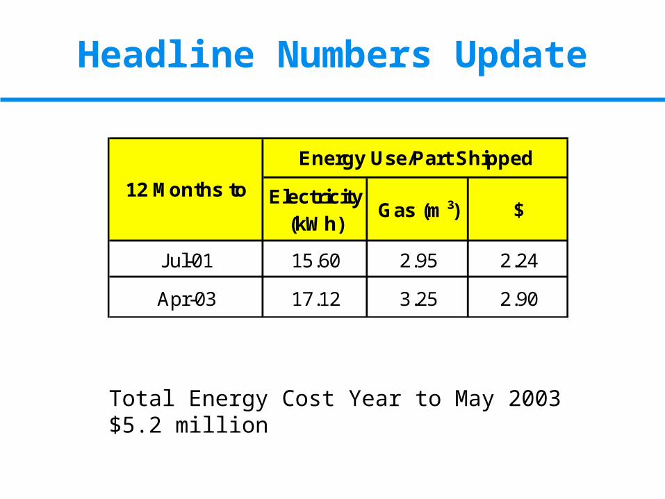
Electricity

(kWh)Gas (m³) $

Jul-01 15.60 2.95 2.24

Apr-03 17.12 3.25 2.90

Energy Use/Part Shipped

12 Months to

Total Energy Cost Year to May 2003 $5.2 million

Headline Numbers Update

Electricity Cost By Department

Colour Line

Compressors

Chillers

Site Utilities

South Warehouse

RTO Unit

Test Laboratory

Prime Line

North Warehouse

Total Cost from 13/01/2003 to 08/05/2003

$1,789,556

$1,444,140

$1,427,079

$1,413,034

$392,723

$359,454

$339,292

$332,951$194,298

Utility Management

• In 2001, utility consumption data was very poor

• Metering is now excellent

• The only significant gap is the RTO

• Environmental drivers are more powerful

• Montage, Powerlogic and ORCI all provide excellent data

Priority Areas

• Compressed air

• Chillers

• RTO

• Colour Line

Air compressors

• Well metered

• Annual energy consumption is 5.3 million kWh/year ($480,000)

• Centacs now meet all demand

• One machine is shutdown at weekends

• Manual control

$1400/day

$700/day

0

100

200

300

400

500

600

700

800

01.0

5.03

02.0

5.03

03.0

5.03

04.0

5.03

05.0

5.03

06.0

5.03

07.0

5.03

08.0

5.03

09.0

5.03

10.0

5.03

11.0

5.03

12.0

5.03

13.0

5.03

kW

E Broomwade

E Centac Units

E XLE-1

E XLE-2

Total

$1400/day

$970/day

Air Compressors Hourly Electricity Use

• Run a Centac and the Broomwade - estimated saving $150,000/year

• Just run the Broomwade at night and weekends estimated saving $30,000

• When Prime Line restarts investigate a heat regenerated drier

Scope for Savings

Chillers

• Chillers, pumps and CTs consume 6 million kWh/year ($550,000)

• 1 chiller in the winter and 2 in the summer

• System is oversized and inflexible

• In the winter cooling load from ASH is 74kW (+90kW from old compressors) actual cooling is 750kW and compressor power is 350kW i.e. effective COP of 0.4

0

5

10

15

20

25

30

35

01-J

un-0

2

08-J

un-0

2

15-J

un-0

2

22-J

un-0

2

29-J

un-0

2

06-J

ul-0

2

13-J

ul-0

2

20-J

ul-0

2

27-J

ul-0

2

03-A

ug-0

2

10-A

ug-0

2

17-A

ug-0

2

24-A

ug-0

2

31-A

ug-0

2

07-S

ep-0

2

14-S

ep-0

2

21-S

ep-0

2

28-S

ep-0

2

05-O

ct-0

2

12-O

ct-0

2

19-O

ct-0

2

Ave

rag

e T

emp

deg

C

0

5000

10000

15000

20000

25000

30000

35000

40000

45000

kWh

/day

Mean Temp

Chiller kWh

Chillers – Daily Elec. Use and Average Temperature

3 Pumps 4 Pumps

2 Pumps

5 Pumps

6 Pumps

Chillers Potential Savings

• In the summer one chiller is switched off at weekend

• Corresponding pumps are not always switched off – potential saving 60,000 kWh/year ($5,400)

• Can a chiller be switched off at night in the summer 3hrs@50 days – potential savings 60,000 kWh/year ($5,400)

• VFD for glycol pumps

• Small chiller for winter

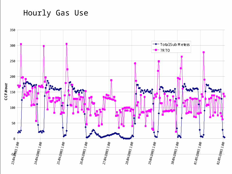
RTO

• Meter has not yet been configured

• Estimated gas use $1.4 million/year

• Electricity use of RTO fan 1.6 million kWh/year ($140,000)

• Control of flow and LEL to the RTO is essentially manual

-50

0

50

100

150

200

250

300

350

23/0

4/20

03 1

:00

24/0

4/20

03 1

:00

25/0

4/20

03 1

:00

26/0

4/20

03 1

:00

27/0

4/20

03 1

:00

28/0

4/20

03 1

:00

29/0

4/20

03 1

:00

30/0

4/20

03 1

:00

01/0

5/20

03 1

:00

02/0

5/20

03 1

:00

CC

F/H

ou

r

Total Sub Meters

?RTO

Hourly Gas Use

RTO Savings Potential

• Weekend setting for night non productive time estimated saving 280,000 m³/year ($90,000) for gas and 50,000 kWh/year ($4,500) for electricity

• Optimization of LEL set points (and air flows) Saving ?$100,000/year

Colour Line

• Is comprehensively metered

• Total gas cost is $400,000/year

• Total electricity is $600,000/year

• Is well controlled

0

5

10

15

20

25

3795

6.79

167

3795

6.95

834

1/13

/03

3:00

:00

AM

1/13

/03

7:00

:00

AM

1/13

/03

11:0

0:01

AM

1/13

/03

3:00

:01

PM

1/13

/03

7:00

:01

PM

1/13

/03

11:0

0:00

PM

1/14

/03

3:00

:01

AM

1/14

/03

7:00

:00

AM

1/14

/03

11:0

0:00

AM

1/14

/03

3:00

:01

PM

1/14

/03

7:00

:01

PM

1/14

/03

11:0

0:01

PM

1/15

/03

3:00

:00

AM

1/15

/03

7:00

:01

AM

1/15

/03

11:0

0:01

AM

1/15

/03

3:00

:00

PM

1/15

/03

7:00

:00

PM

1/15

/03

11:0

0:01

PM

1/16

/03

3:00

:00

AM

1/16

/03

7:00

:01

AM

1/16

/03

11:0

0:00

AM

1/16

/03

3:00

:01

PM

1/16

/03

7:00

:01

PM

1/16

/03

11:0

0:01

PM

1/17

/03

3:00

:00

AM

1/17

/03

7:00

:01

AM

1/17

/03

11:0

0:00

AM

1/17

/03

3:00

:01

PM

CC

F/h

ou

r

G Colour DryoffG Colour Radiant Zone 2G Colour Oven Zone 3G Colour Oven Zone 4G Colour Radiant Zone 2G Colour Radiant Zone 1G Colour Wash Stg1 - B#1G Colour Wash Stg1 - B#1

Colour Line Hourly Gas Use

Colour Line Hourly Electricity Use kW

-50

0

50

100

150

200

250

300

350

400

450

500 E Colour Clear Ash

E Colour Washline

Thurs Fri Sat Sun Mon Tues Weds Thurs Fri Sat Sun Mon

Colour Line Gas Savings Potential

• Appears well controlled

• Improving shut down and start up procedure would save $3-4000/year for gas and $6,000 for electricity

Potential Savings

Colour Shutdown $10,000

Compressed air $180,000

Glycol Pumps $5,400

Chiller switch off $5,400

RTO $190,000

Total $391,000

Other significant areas are lighting and space heating

Conclusions

• Level of data is very impressive

• Major gaps are:

> RTO

>Main site gas meter

>Correlate chiller performance to ambient conditions and/or COP

• Next step is to analyse and act upon the data