The Flash ADC system and PMT waveform reconstruction for the Daya BayExperiment

Yongbo Huanga,b, Jinfan Changa,c, Yaping Chenga, Zhang Chena,b, Jun Hua,c, Xiaolu Jia,c, Fei Lia,c, Jin Lia,b,c, Qiuju,Lia,c, Xin Qiane, Jetter Soerena, Wei Wangd, Zheng Wanga,c, Yu Xud, Zeyuan Yua,∗

aInstitute of High Energy Physics, Beijing 100049, ChinabUniversity of Chinese Academy of Sciences, Beijing 100049, China

cState Key Laboratory of Particle Detection and Electronics, Beijing 100049, ChinadSun Yet-Sen University, Guangzhou 510275, China

ePhysics Department, Brookhaven National Laboratory, Upton, NY, USA

Abstract

To better understand the energy response of the Antineutrino Detector (AD), the Daya Bay Reactor Neutrino Experi-ment installed a full Flash ADC readout system on one AD that allowed for simultaneous data taking with the currentreadout system. This paper presents the design, data acquisition, and simulation of the Flash ADC system, and focuseson the PMT waveform reconstruction algorithms. For liquid scintillator calorimetry, the most critical requirement towaveform reconstruction is linearity. Several common reconstruction methods were tested but the linearity perfor-mance was not satisfactory. A new method based on the deconvolution technique was developed with 1% residualnon-linearity, which fulfills the requirement. The performance was validated with both data and Monte Carlo (MC)simulations, and 1% consistency between them has been achieved.

Keywords: Flash ADC, Waveform reconstruction, Daya Bay ExperimentPACS: 85.60.Ha, 14.60.Pq

1. Introduction

The Daya Bay Reactor Neutrino Experiment pro-vided the world’s most precise measurement of sin22θ13and the effective squared mass splitting |∆m2

ee| [1]. Aprecise measurement of the reactor anti-neutrino spectrawas also reported [2]. Both analyses require a good un-derstanding of the Antineutrino Detector’s (AD) energyresponse, that is the relationship between the energy ofthe ν̄e and the reconstructed energy of the positron, thefinal-state lepton of the Inverse Beta Decay (IBD) reac-tion (Eq. 1).

ν̄e + p = e+ + n (1)

Liquid scintillator (LS) has been used in calorimetersfor several decades. It is also utilized by Daya Bay asthe ν̄e target and detector. The positron from an IBD re-action deposits its kinetic energy then annihilates withan electron creating two γ-rays in the LS. The deposited

∗Corresponding author. Tel:+86-10-8823-6256.Email address: yuzy@ihep.ac.cn (Zeyuan Yu )

energy is converted to scintillation light. It has been es-tablished that scintillation light production is not linearwith the deposited energy, due to ionization quenchingand contributions from Cherenkov light[3], referred toas LS non-linearity.

The scintillation light is detected by photomultipliertubes (PMTs). The PMT output analog signal is pro-cessed by custom front-end electronics designed by theDaya Bay collaboration, giving the integrated chargeand a time stamp. Daya Bay utilizes a CR-(RC)4 shap-ing circuit to integrate the PMT signal that possessesa complex interplay with the scintillation timing pro-file, which consists of three exponential decayed com-ponents: a fast one with a time-constant of less than 10ns, a medium one with a time-constant of about 30 ns,and a slow one with a time-constant larger than 150 ns.This interplay creates a non-linear relationship betweenthe PMT’s received photons and the integrated charge,referred to as electronic non-linearity, which is about10% from 1 p.e. to 10 p.e. for Daya Bay [1].

Coupling between the particle-dependent LS non-linearity and energy-dependent electronic non-linearity

Preprint submitted to Nucl. Instr. Meth. A April 10, 2018

arX

iv:1

707.

0369

9v2

[ph

ysic

s.in

s-de

t] 9

Apr

201

8

introduces difficulties to the precise understanding ofthe detector energy response. To de-couple them, aFlash Analog Digital Convertor (FADC) readout systemwas installed for AD1 in the Daya Bay Experiment Hall.Simultaneous data taking with the current readout sys-tem began in Feb. 2016.

The PMT’s waveform recorded by the FADC inprinciple allows for the precise reconstruction of PMTcharge and a measurement of the electronics non-linearity. However, due to the coupling of Daya BayPMTs’ overshoot and the LS scintillation timing, theprecise charge extraction is not trivial. The scientificgoal requires the non-linearity of PMT charge recon-struction to be no more than 1%, which controls the sizeof electronics non-linearity to less than 0.3%.

This paper presents the design, data acquisition(DAQ), and simulation of the FADC system. Severalwaveform reconstruction methods were developed andtested, but the 1% linearity requirement was not satisfiedinitially. Then a fast, robust and precise charge recon-struction algorithm was developed based on the decon-volution technique with 1% non-linearity as estimatedfrom MC. To validate the results, data and MC werecompared achieving agreement at 1% level.

2. Flash ADC system

2.1. System design

In Daya Bay, each AD contains 192 HamamatsuR5912 8” PMTs, operating under positive high voltages(HV). The HV and PMT output signal share the samecable, and to decouple them, a custom-built splitter fil-ters the high voltage. The analog signal is passed to thefront-end electronics (FEE). Details of the current read-out system are reported elsewhere [4].

The signal distribution scheme to the newly installedFADC system is shown in Fig. 1.

Figure 1: Signal distribution scheme to the Daya Bay FADC system.PMT signals were sent into a FIFO with two outputs. One output wasfed into the old electronics named FEE, and the other one with 10times amplification was fed into the new FADC system.

To enable FEE and FADC simultaneously data tak-ing, a Fan-In-Fan-Out (FIFO) system with 192 channelswas built. The PMT signals from the splitter are fed intothe FIFO with two outputs. One output with 1x amplifi-cation is sent to the FEE, and the other one with 10x am-plification is sent to the FADC. The chip used in the firstoutput (for the FEE) is ADA4817, with a -3 dB band-width 1.05 GHz. The second output uses the AD8000,chip with a -3 dB bandwidth 1.5 GHz. Both amplifiersare fast enough to prevent distortions, since the signalsconcentrated in the frequency range less than 300 MHz.

The custom-built FADC system consists of twelveboards with 192 channels in total. The ADC chip oper-ating with a sampling rate of 1 GHz, an effective num-ber of bits (ENOB) of 7.8, and a maximum range of 500mV. The main function of the high speed ADC moduleis signal conditioning, high speed AD conversion, datacapture and transmitting the interesting data to the DAQaccording to the trigger signal. The module is based onthe daughter-mother board structure and both boards are8 layers pcb. The structure of this module is shown inFig. 2. The daughter board is based on a 4-channel, 1GSps, 10-bit ADC chip and the model is EV10AQ190.

To provide high performance 1 GHz clock to ADC, aHMC830LP6GE jitter cleaner is used. The analog sig-nal from the detector is converted into a differential sig-nal through a high speed amplifier and then transferredto the ADC chip. The FPGA captures the ADCs outputdigital data. After receiving a trigger signal, the FPGApackages the interesting data and transmits it to DAQserver.

The mother board is a 9U-VME board. It collectsthe raw data from 4 daughter boards and transmits themto the data acquisition system via gigabit Ethernet withTCP/IP protocol. It also receives the trigger signaland fans it out to all the ADC daughter boards. A re-mote update circuit based on CPLD makes updating thefirmware of the system convenient. As the key com-ponent in this system, FPGA is Xilinx XC5VSX50Twhich contains enough logic, ram and interface resourcefor the data transmitting, especially DSP resource forthe complex signal processing algorithm in the future.

The readout window length is configurable from 100ns to 100 µs, and was chosen to be 1008 ns during datataking. The window length is chosen to ensure the over-shoot is well recovered while minimizing the data vol-ume.

The trigger of FADC and FEE comes from the sametrigger board. Trigger signal from the trigger board goesto a Fan-In-Fan-Out (FIFO) board which is installed onthe crate of FEE. The FIFO has more than ten outputswhich are sent to each FEE board and FADC board.

2

And the cables connecting the FIFO and FEE/FADChave the same length. So the FADC system shared thesame trigger and global time with the FEE. Both FEEand FADC events contain global trigger time stampswhich could be used to align the events recorded by twosystems.

Figure 2: Photograph of one FADC board consisting of 16 channels.The mother board is a 9U-VME board. It collects the raw data from 4daughter boards.

An example waveform taken by the FADC system isshown in Fig. 3. The amplitude of a single p.e. is about40 mV (about 80 ADC counts) after 10x amplification.Frequency analysis shows that signals concentrated toless than 300 MHz, which is due to the PMT itself,and the electronics noise was almost white, as shownin Fig. 4. It can be concluded that the FADC designfulfilled the Sampling Theorems [5] and QuantisationTheorems [6].

Since the Daya Bay experiment utilizes the near andfar relative measurement to measure the neutrino mix-ing angle θ13, it was critical to prevent FEE response dif-ferences before and after the FADC installation. Manychecks were done to demonstrate that the FEE wasworking as before, including PMT gains, dark rates,measured charge and time spectra, etc. Nothing abnor-mal was found, indicating that the relative ν̄e detectionefficiencies between AD1 and the other ADs was notaffected.

2.2. Data acquisitionAlthough benefiting from a high sampling rate, huge

data volumes are a significant issue for experiments em-ploying FADCs. Data of the FADC system at Daya Bay

Time [ns]50 100 150 200 250 300 350 400 450 500

AD

C

0

50

100

150

200

Figure 3: One PMT waveform with pile-up hits from data. Amplitudeof a single p.e. was about 80 ADC counts (40 mV). The overshootcame from the PMT base and the HV-signal splitter.

Figure 4: Frequency response of the FADC data. The red solid lineis the sum of PMT signals and noise, and the black dash line is pureelectronics noise.

were sent to the new DAQ via Ethernet, the raw triggerrate of the FADC system was about 240 Hz, generating80 MB/s of raw data, which was much larger than the 20MB/s network bandwidth between the experiment siteand the offline computing center. An effective data re-duction strategy was therefore developed.

The DAQ scheme and its implementation was re-ported elsewhere [7]. The DAQ program was further de-veloped for the data reduction which consisted of threesteps [8].

1) Time correlation cut. The DAQ recorded onlyevent pairs within a time interval less than 0.5 ms. Thiseliminates most of the single events from natural ra-dioactivity, keeping the events of interest, for example,Inverse Beta Decay and Bi-Po cascade decays. Afterthis step, the trigger rate and data size are decreased to30 Hz and 10 MB/s, respectively.

2) Energy cut. A prompt energy reconstruction was

3

done in the DAQ program. Events with an energy lessthan 0.6 MeV or larger than about 15 MeV are removed.The trigger rate and data size were further reduced to 13Hz and 5 MB/s.

3) Empty channel cut. In each event, if a channel didnot pass a 0.3 p.e. threshold, it was removed, resultingin a 2 MB/s data size.

The time correlation cut is done on the FADC board,DAQ program doesn’t read events which don’t pass thiscut. The other cuts are done in the memory of DAQserver, before writing data to hard disk. With this effec-tive data reduction algorithm, the data size fulfilled therequirements for the data transferring from Daya Bay tothe computing center.

3. FADC simulation

To model the FADC responses and validate the PMTcharge reconstruction algorithms, a precise single chan-nel electronics simulation was developed, with the fol-lowing steps.

1) Sample the PMT hit number and time. The hitnumber distribution was user defined, i.e. physical oruniformly distributed. The time of each hit was sampledfrom the measured LS scintillation timing profile.

2) Convolve the hits with analog PMT single p.e.waveform, which was modeled by a data-driven func-tion, to be discussed in Sec. 3.1. The amplitude of singlep.e. followed a Gaussian distribution with 30% resolu-tion according to the real PMT response.

3) Add analog electronics noise and the baseline off-set. White noise with 0.7 mV sigma and measured noisefrom Daya Bay FADC data were tested, and no differ-ences were found.

4) Digitization. The analog waveform was digitizedwith the FADC configurations, following the round off

principle.

3.1. Single p.e. waveform modeling

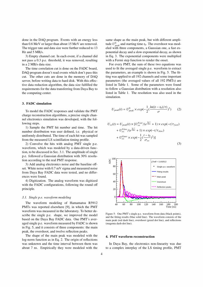
The waveform modeling of Hamamatsu R5912PMTs was reported elsewhere [9], in which the PMTwaveform was measured in the laboratory. To better de-scribe the single p.e. shape, we improved the modelbased on the Daya Bay FADC data. One PMT’s aver-aged single p.e. waveform measured by FADC is shownin Fig. 5, and it consists of three components: the mainpeak, the overshoot, and twelve reflection peaks.

The shape of the main peak was modeled with thelog-norm function as in Eq. 2. The origin of reflectionswas unknown and the time interval between them wasabout 7 ns. Empirically they were modeled with the

same shape as the main peak, but with different ampli-tude U0

peak and starting time t0. The overshoot was mod-eled with three components, a Gaussian one, a fast ex-ponential decay and a slow exponential decay, as shownin Eq. 3. The exponential components were multipliedwith a Fermi step function to render the onset.

For every PMT, the sum of these two equations wasused to fit the averaged single p.e. waveform to extractthe parameters, an example is shown in Fig. 5. The fit-ting was applied to all 192 channels and some importantparameters (the averaged values of all 192 PMTs) arelisted in Table 1. Some of the parameters were foundto follow a Gaussian distribution with a resolution alsolisted in Table 1. The resolution was also used in thesimulation.

Upeak(t) = U0peak × exp(−

12

(ln((t − t0)/τ)

σ)2) (2)

Uos(t) = Upeak(t) × [UFastos /(e

t0−t10ns + 1) × exp(−t/τ f ast)

+ US lowos /(e

t0−t10ns + 1) × exp(−t/τslow)

+ UGausos × exp(−

12

(t − t0σos

)2)]

(3)

Time [ns]40 60 80 100 120 140 160 180 200

AD

C

0

20

40

60

80

100/ndf = 1143/5122χ

Single p.e. waveform

Fitting results

Main peak

Overshoot

Reflection peaks

Figure 5: One PMT’s single p.e. waveform from data (black points),and the fitting results (blue solid line). The waveform consists of themain peak (red dash line), overshoot (greed dot line), and reflections(magenta dash-dot line).

4. PMT waveform reconstruction

In Daya Bay, the electronics non-linearity was dueto a complex interplay of the LS timing profile, PMT

4

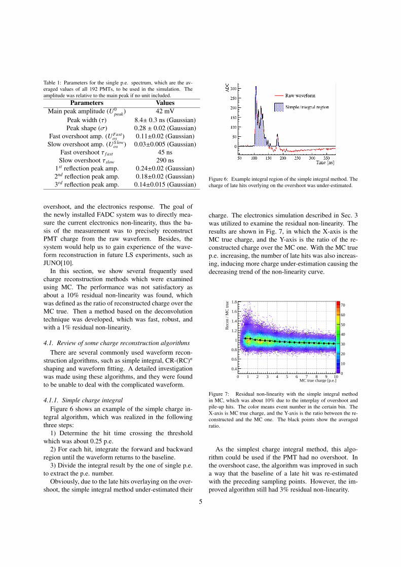
Table 1: Parameters for the single p.e. spectrum, which are the av-eraged values of all 192 PMTs, to be used in the simulation. Theamplitude was relative to the main peak if no unit included.

Parameters ValuesMain peak amplitude (U0

peak) 42 mVPeak width (τ) 8.4± 0.3 ns (Gaussian)Peak shape (σ) 0.28 ± 0.02 (Gaussian)

Fast overshoot amp. (UFastos ) 0.11±0.02 (Gaussian)

Slow overshoot amp. (US lowos ) 0.03±0.005 (Gaussian)

Fast overshoot τ f ast 45 nsSlow overshoot τslow 290 ns

1st reflection peak amp. 0.24±0.02 (Gaussian)2nd reflection peak amp. 0.18±0.02 (Gaussian)3rd reflection peak amp. 0.14±0.015 (Gaussian)

overshoot, and the electronics response. The goal ofthe newly installed FADC system was to directly mea-sure the current electronics non-linearity, thus the ba-sis of the measurement was to precisely reconstructPMT charge from the raw waveform. Besides, thesystem would help us to gain experience of the wave-form reconstruction in future LS experiments, such asJUNO[10].

In this section, we show several frequently usedcharge reconstruction methods which were examinedusing MC. The performance was not satisfactory asabout a 10% residual non-linearity was found, whichwas defined as the ratio of reconstructed charge over theMC true. Then a method based on the deconvolutiontechnique was developed, which was fast, robust, andwith a 1% residual non-linearity.

4.1. Review of some charge reconstruction algorithmsThere are several commonly used waveform recon-

struction algorithms, such as simple integral, CR-(RC)n

shaping and waveform fitting. A detailed investigationwas made using these algorithms, and they were foundto be unable to deal with the complicated waveform.

4.1.1. Simple charge integralFigure 6 shows an example of the simple charge in-

tegral algorithm, which was realized in the followingthree steps:

1) Determine the hit time crossing the thresholdwhich was about 0.25 p.e.

2) For each hit, integrate the forward and backwardregion until the waveform returns to the baseline.

3) Divide the integral result by the one of single p.e.to extract the p.e. number.

Obviously, due to the late hits overlaying on the over-shoot, the simple integral method under-estimated their

Figure 6: Example integral region of the simple integral method. Thecharge of late hits overlying on the overshoot was under-estimated.

charge. The electronics simulation described in Sec. 3was utilized to examine the residual non-linearity. Theresults are shown in Fig. 7, in which the X-axis is theMC true charge, and the Y-axis is the ratio of the re-constructed charge over the MC one. With the MC truep.e. increasing, the number of late hits was also increas-ing, inducing more charge under-estimation causing thedecreasing trend of the non-linearity curve.

MC true charge [p.e.]0 1 2 3 4 5 6 7 8 9 10

Rec

on /

MC

true

0.4

0.6

0.8

1

1.2

1.4

1.6

1.8

0

10

20

30

40

50

60

70

Figure 7: Residual non-linearity with the simple integral methodin MC, which was about 10% due to the interplay of overshoot andpile-up hits. The color means event number in the certain bin. TheX-axis is MC true charge, and the Y-axis is the ratio between the re-constructed and the MC one. The black points show the averagedratio.

As the simplest charge integral method, this algo-rithm could be used if the PMT had no overshoot. Inthe overshoot case, the algorithm was improved in sucha way that the baseline of a late hit was re-estimatedwith the preceding sampling points. However, the im-proved algorithm still had 3% residual non-linearity.

5

4.1.2. CR-(RC)n shapingThe CR-(RC)n shaping method for charge reconstruc-

tion was also investigated. It improved the Signal-to-Noise ratio, but increased the pulse width, induced bypulse pile-up and affected the charge measurement. Ifthe signals’ arrival time was concentrated to less than 20ns, the shaping could give a linear charge measurement.In the LS detector, which had medium and slow scintil-lation components, the shaping seemed not proper.

Figure 8: Left: the black solid line is the simulated waveform oftwo simultaneous hits and the red dashed line is that of the same twohits separated by 30 ns, both without electronics noise. Right: thetwo waveforms after CR-(RC)4 shaping. The separated hits have aunder-estimated charge, which is 6753 and about 5% lower than thatof simultaneous hits.

MC true charge [p.e.]0 1 2 3 4 5 6 7 8 9 10

Rec

on /

MC

true

0

0.2

0.4

0.6

0.8

1

1.2

1.4

1.6

1.8

2

0

5

10

15

20

25

30

35

40

45

Figure 9: Residual non-linearity of CR-(RC)4 shaping, about 10%,due to the complex interplay between the shaping constant, overshootand LS scintillation timing.

Since the current Daya Bay electronics was designedwith the CR-(RC)4 shaping circuit, with the τ of eachCR or RC of 25 ns, we chose n=4 as an example . PMTcharge was reconstructed with a peak finding algorithmafter the CR-(RC)4 circuit, and the integral value wasapproximated as peak height. As shown in Fig. 8, if twohits were separated by 30 ns, the reconstructed chargewas under-estimated by 5% compared to the case of thesame two simultaneous hits. With the time separationincreasing, the under-estimation was also increasing.

With electronics simulation the residual non-linearitywas studied and is shown in Fig. 9, which was also about10%.

4.1.3. Waveform fittingTo reconstruct the late hits better, a waveform fitting

algorithm was developed, which utilized the calibratedsingle p.e. waveform as a template. A fitting exampleis shown in Fig. 10. Although the residual non-linearitywas improved to about 2%, the algorithm had two short-ages to overcome.

/ ndf 2χ 936.3 / 490Prob 2.672e-30

Time [ns]0 50 100 150 200 250 300 350

AD

C

-50

0

50

100

150

200

250 / ndf 2χ 936.3 / 490Prob 2.672e-30

Figure 10: An example of waveform fitting. Late hits could be wellreconstructed, but the fitting speed was a significant problem with 0.5s per waveform.

The first one was speed. The fitting of one waveformrequired about 0.5 second, which was a huge workloadduring the data reconstruction.

The second one was fitting quality. The fitting hada increasing failure rate with increasing number of hits,introducing a residual non-linearity which was difficultto calibrate.

The waveform fitting method could be used in thecrosscheck analysis of small event samples, for exam-ple, Inverse Beta Decays, etc., in which special carecould be taken to examine the fitting quality.

4.2. A method with the deconvolution technique

Deconvolution is a well-developed and widely usedtechnique in Digital Signal Processing (DSP) [12]. Itis also utilized in various physics experiments, for ex-ample, to extract correct information from pile-up [13],pattern recognition [14], and energy spectrum study[15]. Furthermore, we found that deconvolution was apowerful tool to reconstruct the PMT charge with goodlinearity, especially in the case when signals were bi-polar and overlapping.

In the time domain the deconvolution was not easyto process, but in the frequency domain it was rather

6

simple. The raw waveform was converted to the fre-quency domain with Discrete Fourier Transform (DFT),then multiplied with a noise filter, divided by the fre-quency response of a calibrated single p.e. waveform,and finally converted to the time domain with InverseDFT. The DFT and Inverse DFT were done with the FastFourier Transform package in the data analysis frame-work ROOT [11].

There were a lot of noise filters in the DSP, such asOptimized Wiener Filter, Windowed-Sinc Filter, Gaus-sian Filter etc [12]. They were investigated, and acustom-defined low-band pass filter was adopted, asshown in Fig. 11.

Frequency [MHz]0 50 100 150 200 250 300 350 400 450 500

Filte

r

0

0.2

0.4

0.6

0.8

1

2)40

x-100*(21-

e

Figure 11: The custom-defined low-band pass filter. In case of lessthan 100 MHz, the filter response equals to 1, while larger than 300MHz is 0. Between 100 MHz to 300MHz, the filter is described withthe Gaussian formula as shown in the plot.

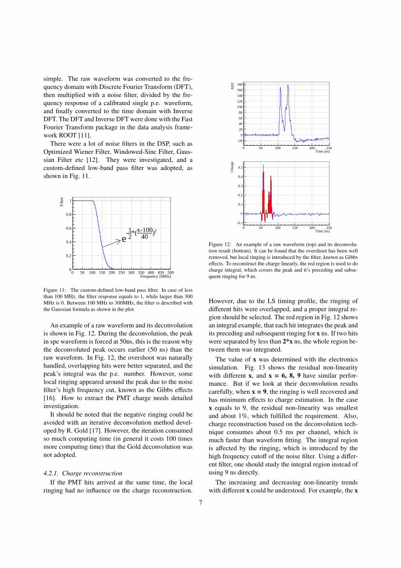
An example of a raw waveform and its deconvolutionis shown in Fig. 12. During the deconvolution, the peakin spe waveform is forced at 50ns, this is the reason whythe deconvoluted peak occurs earlier (50 ns) than theraw waveform. In Fig. 12, the overshoot was naturallyhandled, overlapping hits were better separated, and thepeak’s integral was the p.e. number. However, somelocal ringing appeared around the peak due to the noisefilter’s high frequency cut, known as the Gibbs effects[16]. How to extract the PMT charge needs detailedinvestigation.

It should be noted that the negative ringing could beavoided with an iterative deconvolution method devel-oped by R. Gold [17]. However, the iteration consumedso much computing time (in general it costs 100 timesmore computing time) that the Gold deconvolution wasnot adopted.

4.2.1. Charge reconstructionIf the PMT hits arrived at the same time, the local

ringing had no influence on the charge reconstruction.

Time [ns]0 50 100 150 200 250

AD

C

-20

0

20

40

60

80

100

120

140

160

180

Time [ns]0 50 100 150 200 250

Cha

rge

-0.1

0

0.1

0.2

0.3

0.4

0.5

Figure 12: An example of a raw waveform (top) and its deconvolu-tion result (bottom). It can be found that the overshoot has been wellremoved, but local ringing is introduced by the filter, known as Gibbseffects. To reconstruct the charge linearly, the red region is used to docharge integral, which covers the peak and it’s preceding and subse-quent ringing for 9 ns.

However, due to the LS timing profile, the ringing ofdifferent hits were overlapped, and a proper integral re-gion should be selected. The red region in Fig. 12 showsan integral example, that each hit integrates the peak andits preceding and subsequent ringing for x ns. If two hitswere separated by less than 2*x ns, the whole region be-tween them was integrated.

The value of x was determined with the electronicssimulation. Fig. 13 shows the residual non-linearitywith different x, and x = 6, 8, 9 have similar perfor-mance. But if we look at their deconvolution resultscarefully, when x = 9, the ringing is well recovered andhas minimum effects to charge estimation. In the casex equals to 9, the residual non-linearity was smallestand about 1%, which fulfilled the requirement. Also,charge reconstruction based on the deconvolution tech-nique consumes about 0.5 ms per channel, which ismuch faster than waveform fitting. The integral regionis affected by the ringing, which is introduced by thehigh frequency cutoff of the noise filter. Using a differ-ent filter, one should study the integral region instead ofusing 9 ns directly.

The increasing and decreasing non-linearity trendswith different x could be understood. For example, the x

7

MC true charge [p.e.]0 2 4 6 8 10

Rec

on /

MC

true

0.95

1

1.05

1.1

1.15Different integral regions

x = 1 nsx = 3 nsx = 6 nsx = 8 nsx = 9 ns

Figure 13: The residual non-linearity of the deconvolution methodwith different x. The blue open circle is x = 9ns which has the bestperformance.

= 0 is expected to only integrate the peak. If there wasone hit, only the peak region was used. If there wereseveral hits overlapping, the peak region of one hit alsooverlapped with the negative ringing of the other hits.Then the ratio between reconstructed charge and truecharge was smaller than in the one hit case, introducingthe decreasing trend. In the bottom plot of Fig. 12, wecan see the ringing is go to finish since 6 ns, thus inte-grate 6, 7, 8 and 9 ns give similar results, as shown inFig. 13.

Since the value of x was determined with MC, to val-idate the results, MC are compared with data, as de-scribed in the next section.

4.3. Summary of the reconstruction algorithms

The interplay between the LS timing profile and PMTovershoot would degrade the performance of two chargereconstruction methods: simple integral and CR-(RC)4

shaping. To pick up the late hits overlaying on the over-shoot of earlier hits, the waveform fitting method wastested, and found too slow to be used in the reconstruc-tion for large data samples. Then an algorithm with thedeconvolution technique was developed. The perfor-mance of these reconstruction algorithms is summarizedin Table 2. It was found that the deconvolution methodis the most powerful tool to deal with the overshoot andoverlapping, and has the smallest residual non-linearity.

Besides the charge measurement, the algorithms haddifferent timing separation abilities for pile-up hits. Thewaveform fitting and deconvolution could discriminatehits separated larger than 10 ns, while for the simpleintegral method it was 20 ns and for the Daya Bay CR-(RC)4 shaping 40 ns.

5. Comparison between electronics simulation anddata

Since the algorithm performance was studied withMC, to validate the conclusions, MC should be com-pared with data. The most direct way was to comparethe residual non-linearity between data and MC, but inthe data there was no true p.e. information. As such, aratio was defined where the deconvolution result withx=9 ns was used as the denominator, and the resultsfrom other methods were used as the numerator. The ra-tio was compared between data and MC, and 1% agree-ments were achieved, indicating confidence in the MCsimulation.

5.1. Comparison of different charge integral methodsfor the deconvolution algorithm

After deconvolution, how to integrate the local ring-ing was studied with MC, and a best solution was givenwhich covered the preceding and subsequent 9 ns. TheMC studies also showed that integrating different re-gions had different non-linearity, which was expectedto be repeated in data.

A ratio was defined as Deconvolution (x = a ns)Deconvolution (x = 9 ns) , where x

meant the integral region, and a ran from 0 to 8. Somecomparison results are shown in Fig. 14 as examples.Data and MC agree to 1%, indicating the MC has welldescribed the waveform and the deconvolution method.

0 2 4 6 8 10

4 ns

/9 n

s

0.95

1

MCData

0 2 4 6 8 10

5 ns

/9 n

s

0.95

1

0 2 4 6 8 10

6 ns

/9 n

s

0.95

1

Deconvolution charge (x=9ns) [p.e.]0 2 4 6 8 10

8 ns

/9 n

s

0.98

1

1.02

Figure 14: Ratio of the reconstructed charge between different chargeintegral regions after deconvolution. Data and MC agree to 1%, indi-cating the MC has well described the waveform and the deconvolutionmethod. The four pads from top to bottom show the ratio of (x = 4, 5,6, 8 ns)/(x = 9 ns) respectively.

5.2. Comparison of different FADC readout windowlengths

The Discrete Fourier Transform assumes that the fi-nite sequence of sample points is periodical. In thewaveform reconstruction, if the overshoot was not wellrecovered at the end of the readout window, the period-ical assumption would treat the un-recovered baselineas a jump. Thus an additional non-linearity would be

8

Table 2: The summary table for different charge reconstruction algorithms.Algorithms Speed per channel Robustness Residual non-linearity Pile-up hits separation

Simple integral less than 0.1 ms No failure 3% to 10% Larger than 20 nsCR-(RC)4 0.2 ms No failure 10% Larger than 40 ns

Waveform fitting 0.5 sSometimes fails and

difficult to define failure 2% Larger than 10 ns

Deconvolution 0.5 ms No failure 1% Larger than 10 ns

induced, and the larger the jump was, the larger non-linearity we got.

The Daya Bay FADC readout window length was setto 1008 ns and the previous results were performed withthis length. To validate the additional non-linearity, thefirst 624 ns was used to reconstruct the PMT charge andcompared to the one reconstructed from the full wave-form. For consistency, both used chose hits with hit timeless than 500 ns for charge reconstruction. As shown inFig. 15, both data and MC showed a decreasing trendand they agreed to better than 1%.

Charge_1008ns [p.e.]1 2 3 4 5 6 7 8 9 10

Cha

rge_

624n

s / C

harg

e_10

08ns

0.975

0.98

0.985

0.99

0.995

1

1.005

1.01Charge_624ns / Charge_1008ns

MC

Data

Figure 15: Ratio of the reconstructed charge between different FADCreadout window lengths. MC and data agree to less than 1%, and thedifferences between 624 ns and 1008 ns are due to the coupling ofDFT’s periodical assumption and the long overshoot.

5.3. Comparison of different reconstruction algorithmsThe simple integral and CR-(RC)4 methods were

more sensitive to the PMT waveform features, such asovershoot, reflections and hit time profiles. Compari-son between them and the deconvolution method couldvalidate the description of waveform features in MC.

Two ratios were defined as S implechargeintegralDeconvolution (x = 9 ns) and

CR−(RC)4

Deconvolution (x = 9 ns) . Data and MC comparison resultsare shown in Fig. 16 and most of them agree to 1%, in-dicating the MC has described the waveform featureswell.

6. Summary

To directly measure the current electronics (FEE)non-linearity, the Daya Bay experiment installed a Flash

1 2 3 4 5 6 7 8 9 10

Rat

io

0.860.880.9

0.920.940.960.98

11.021.041.06

DeconvolutionSimple Integral

Ratio = MC

Data

Deconvolution charge (x=9ns) [p.e.]1 2 3 4 5 6 7 8 9 10

Rat

io

0.860.880.9

0.920.940.960.98

11.021.041.06

Deconvolution

4CR-(RC)Ratio =

Figure 16: Top: comparison between the simple integral method andthe deconvolution one; bottom: between the CR-(RC)4 shaping andthe deconvolution one. Most of the points agree to 1% indicating theMC has described the waveform features well.

ADC system on AD1. The system has been stably run-ning since Feb. 2016, and no influence was found to theFEE. The scientific goal required a precise PMT chargereconstruction algorithm, and several waveform recon-struction methods were developed and examined. Theone based on the deconvolution technique was foundto have the best performance, with a 1% residual non-linearity. A confident electronics simulation was de-veloped and it agreed with data to 1%. In particular,the FADC data, combined with the developed deconvo-lution charge reconstruction method validate the elec-tronics non-linearity modeling currently implementedin Daya Bays oscillation [1] [18] and reactor physicsanalyses [2].

This work has been supported by the National NaturalScience Foundation of China (11390385).

References

[1] F.P. An et al, Daya Bay Collaboration, Measurement of elec-tron antineutrino oscillation based on 1230 days of operationof the Daya Bay experiment, Phys. Rev. D 95 (072006). doi:10.1103/PhysRevD.95.072006.

[2] F.P. An et al, Daya Bay Collaboration, Measurement of the Re-actor Antineutrino Flux and Spectrum at Daya Bay, Phys. Rev.Lett. 116 (061801). doi: 10.1103/PhysRevLett.116.061801.

[3] J.B. Birks et al, The Theory and Practice of Scintillation Count-ing, 1964.

[4] F.P. An et al, Daya Bay Collaboration, The Detector System ofThe Daya Bay Reactor Neutrino Experiment, Nucl. Instr. Meth.A 811 (2016) 133-161. doi: 10.1016/j.nima.2015.11.144.

9

[5] B. Widrow et al, Statistical theory of quantization, IEEE Trans.Instrumentation and Measurement 45 (2) (1996) 353-361. doi:10.1109/19.492748.

[6] B. Widrow, Quantization Noise: Roundoff Error in DigitalComputation, Signal Processing, Control, and Communications,Cambridge University Press, 2010.

[7] F. Li et al, DAQ Architecture Design of Daya Bay Reactor Neu-trino Experiment, IEEE Transactions on Nuclear Science 58 (4)(2011) 1723-1727. doi: 10.1109/TNS.2011.2158657.

[8] J. Li et al, The Designation of the Waveform Data DAQ Soft-ware for Daya Bay Neutrino Experiment, Nuclear Electronicsand Detection Technology 36 (10) (2016) 1032-1036.

[9] S. Jetter et al, PMT Waveform Modeling at the Daya BayExperiment, Chinese Physics C 36 (8) (2012) 733-741. doi:10.1088/1674-1137/36/8/009.

[10] F.P. An et al, JUNO Collaboration, Neutrino Physicswith JUNO, J. Phys. G 43 (030401). doi: 10.1088/0954-3899/43/3/030401.

[11] R. Brun and F. Rademakers, ROOT - An Object Oriented DataAnalysis Framework, Proceedings AIHENP’96 Workshop, Lau-sanne, Sep. 1996, Nuclear Instruments and Methods in PhysicsResearch A 389 (1997) 81-86. http://root.cern.ch/

[12] S.W. Smith, The Scientist and Engineer’s Guide to Digital Sig-nal Processing, California Technical Pub, 1997.

[13] W. Xiao et al, Model-based pulse deconvolution method forNaI(Tl) detectors, Nucl. Instr. Meth. A 769 (1) (2015) 5-8. doi:10.1016/j.nima.2014.09.034.

[14] M. Miroslav et al, Method of identification of rings in spec-tra from RICH detectors using a deconvolution-based patternrecognition algorithm, Nucl. Instr. Meth. A 639 (1) (2011) 249-251. doi: 10.1016/j.nima.2010.09.059.

[15] M. Neuer, Spectral identification of a 90Sr source in the pres-ence of masking nuclides using Maximum-Likelihood decon-volution, Nucl. Instr. Meth. A 728 (11) (2013) 73-80. doi:10.1016/j.nima.2013.06.013.

[16] J.W. Gibbs, Fourier’s Series, Nature 59 (1539) (1899) 606. doi:10.1038/059606a0.

[17] R. Gold, An iterative unfolding method for response matrices,AEC Research and Development Report ANL 6984.

[18] F.P. An et al, Daya Bay Collaboration, A new measurement ofantineutrino oscillation with the full detector configuration atDaya Bay, Phys. Rev. Lett. 115 (111802). doi: 10.1103/Phys-RevLett.115.111802.

10