the fuzzy logic method for simpler forecastingcdn.intechweb.org/pdfs/17984.pdf · the fuzzy logic...

The Fuzzy Logic Method for Simpler Forecasting Research Paper

Jeffrey E. Jarrett, Ph.D.* and Jeffrey S. Plouffe, Ph.D. University of Rhode Island *Corresponding author E-mail: [email protected] Received 21 Jan 2011; Accepted 30 Apr 2011

Abstract Fildes and Makridakis (1998), Makridakis and Hibon (2000), and Fildes (2001) indicate that simple extrapolative forecasting methods that are robust forecast equally as well or better than more complicated methods, i.e. Box‐Jenkins and other methods. We study the Direct Set Assignment (DSA) extrapolative forecasting method. The DSA method is a non‐linear extrapolative forecasting method developed within the Mamdani Development Framework, and designed to mimic the architecture of a fuzzy logic control system. We combine the DSA method Winters’ Exponential smoothing. This combination provides the best observed forecast accuracy in seven of nine subcategories of time series, and is the top three in terms of observed accuracy in two subcategories. Hence, fuzzy logic which is the basis of the DSA method often is the best method for forecasting.

1. Introduction Many previous studies of corporate earnings indicated the great desire to forecast earning in a simple manner. Such studies include Elton and Gruber (1972), Brandon and Jarrett (1979), Brandon, Jarrett and Khumuwala (1983, 1986) and Jarrett (1990). A review of many of these studies

and others including an analysis of forecasting accuracy is found in Jarrett and Khumuwala (1987). Later more global studies indicated the great desire for simple methods to forecast earnings and other time series data. Makridakis and Hibon (1979) were one of the first to report that statistically simple extrapolative forecasting to report that statistically simple extrapolative forecasting methods provide forecasts that are at least as accurate as those produced by statistically sophisticated methods. Such a conclusion was in conflict with the accepted view at the time, was not received well by the great majority of scholars. In response to these criticisms Makridakis and Hibon held the M‐Competition (1982), the M2‐Competition (1993) and the M3‐Competition (2000). In each of these additional studies, the major findings of the Makridakis and Hibon (1979) study were upheld and this included the finding concerning the relative accuracy of statistically simple extrapolative methods. In addition to the M‐Competitions, myriad other research, described as accuracy studies, were held utilizing new time series as well as time series from the M‐Competitions, and they confirmed the original findings of Makridakis and Hibon regarding the relative accuracy of extrapolative methods. These studies include, Clements and Hendry, (1989); Lusk and Neves, (1984);

Int. j. eng. bus. manag., 2011, Vol. 3, No. 3, 25-5225 www.intechweb.orgwww.intechopen.com

Int. j. eng. bus. manag., 2011, Vol. 3, No. 3, 25-52

Koehler and Murphree, (1988); Armstrong and Collopy, (1992A and 1992B); Makridakis et al., (1993) and Fildes et al., (1998). The problem as reported by Fildes and Makridakis (1998) and Makridakis and Hibon, (2000) is that many scholars ignored the empirical evidence that accumulated across these competitions on the relative forecast accuracy of various extrapolative methods, under various conditions. Instead they concentrated their efforts on building more statistically sophisticated forecasting methods, without regard to the ability of such methods to accurately predict real‐life data. Makridakis and Hibon (2000) suggest that future research should focus on exploiting the robustness of simple extrapolative methods, that are less influenced by the real life behavior of data, and that new statistically simple methods should be developing. Makridakis‐Hibon suggest that real‐life time series are not stationary, and that many of them also reflect structural changes resulting from the influence of fads and fashions, and that these events can change established patterns in the time series. Moreover, the randomness in business time series is high and competitive actions and reactions cannot be accurately predicted. Also, unforeseen events affecting the series in question can and do occur. In addition, many series are influenced by strong cycles of varying duration and lengths whose turning points cannot be predicted. It is for these reasons that statistically simple methods, which do not explicitly extrapolate a trend or attempt to model every nuance of the time series can and do outperform more statistically sophisticated methods. To analyze the results of Makridakis‐Hibon consider their table below: 2. Fuzzy Logic Mukaidono (2002) concluded, ʺIt is a big task to exactly define, formalize and model complicated systemsʺ, and it is at precisely at this task that fuzzy logic has excelled. In fact, fuzzy logic has routinely been shown to outperform classical mathematical and statistical modeling techniques for many applications involving the modeling of real world data. For example, fuzzy logic has found wide acceptance in the field of systems control. Fuzzy logic has been used in control applications ranging from controlling the speed of small electric motor, to controlling an entire subway system. In nearly every one of these applications fuzzy logic control systems have been shown to outperform more traditional, yet highly advanced, digital control systems. Fuzzy logicʹs success in these applications has been attributed to its ability to effectively model real world

data. Mukaidono (2002) suggests that Fuzzy Logicʹs success lies in the fact that it offers a ʺrougher modeling approachʺ. The process of digital control is somewhat similar to time series extrapolation. In a digital control system, sensors provide a set of quantitative or qualitative observations as input to the controller. The controller in turn models those inputs and provides either a qualitative or quantitative output to the system that is under control. In time series extrapolation, a set of historical observations on a time series, serve as the input data to the forecasting method. The method then produces an output that in the case of time series extrapolation is the forecast or future value of the time series of interest. The differences refer to the control system. With a control system, one utilizes feedback to possibly alter its behavior from time t to time t + Δt. There is no feedback loop built into fuzzy logic models utilized in this study to cover the time period during the horizon. Given the similarities with respect to the task of modeling complex real world data, and the structure of the two modeling systems, a fuzzy logic based method for time series extrapolation would appear to be the type of statistically simple method which Makridakis‐Hibon suggest is suggested.

It is clear from over two decades of research on the relative accuracy of various extrapolative methods that simple methods will in most forecasting situations, and for most data types, produce the most accurate ex ante forecasts. Based on the criterion of accuracy, one will observe in this study that more sophisticated methods, i.e., ARIMA modeling, that fuzzy logic methods are as accurate as the more sophisticated methods and simpler to utilize. In this study there are two major hypotheses. The first hypothesis is that the ex ante forecast accuracy of the DSA method will change in response to changes in the fuzzy set parameter. The fuzzy set parameter is the number of fuzzy sets used to model the time series of interest. The second hypothesis is that the DSA method will provide more accurate ex ante forecasts than the traditional extrapolative forecasting methods to which it has been compared. 3. Research Approach Elton and Gruber (1972), Ried (1972), and Newbold and Granger (1974), were among the first to establish the relative accuracy of different forecasting methods across a large sample of time series. However, these early studies compared only a limited number of methods. Makridakis and Hibon (1979) extended this early work by comparing


the accuracy of a large number of methods across a large number of heterogeneous, real‐life business time series. In 1982 Makridakis et al. (1982) conducted a second accuracy study. In this study the authors invited forecasting experts to participate who had an expertise with a particular extrapolative method, thereby creating a forecasting competition. Since 1982 there have been a number of improvements made to the forecasting competition methodology particularly in terms of predictive and construct validity. The research, which is the subject of this current study, relied on the data, methods and procedures of the M3 Forecasting Competition conducted in 2000 as this competition utilized the most recent advances in the forecasting competition methodology. In this current study, three competitions were required to evaluate the research hypotheses and to establish the relative forecast accuracy of the Direct Set Assignment Method (DSA).

4. Research Hypotheses Research to improve the accuracy of extrapolative methods should focus on the development of statistically simple methods that have the characteristic of being robust to the fluctuations that exist in real world data resulting from both random and non‐random events. Since 1993 studies have been conducted to extend the initial work of Song and Chissom (1993 and 1994), to develop a fuzzy logic method for time series extrapolation. The results of those studies lend empirical support to the theoretical evidence that a fuzzy logic extrapolative method can provide more accurate forecasts than traditional extrapolative methods. Jarrett and Plouffe (2006) suggest in their conclusion that improving the accuracy of these methods requires that a new fuzzy logic extrapolative method be developed that will have the implicit ability too provide accurate forecasts of times series in which a trend or seasonal component is present, without the need to decompose the time series. Additionally, this method should allow for fuzzy set parameters other than seven. In response, a new fuzzy logic method for time series extrapolation has been developed and introduced in this research. This method builds on the work of Song and Chissom (1993 and 1994) and Chen (1996). This new method has a new fuzzifier module that allows for scalar values to be simply and directly assigned to fuzzy sets. This module will also capture a trend if one exists in the time series, and further it allows the modeler to specify the value of the fuzzy set parameter.

In addition, the inference module from the earlier methods has been modified to capture the seasonal component, of any duration, and a new defuzzifier module has been created that uses the center‐of‐sets principle. Finally the composition module, that uses Mamdani fuzzy logic relationships, which was used successfully in the Chen method has been retained in the Direct Set Assignment method. Three forecasting competitions have been designed to validate the relative accuracy of the Direct Set Assignment method. These competitions have used, as required, for each competition, the data, accuracy measures, procedures and best performing simple extrapolative methods from the M3‐Competition, Makridakis‐Hibon. To investigate the effect of and changes to fuzzy set parameter, in this study, two null hypotheses will be tested:

HO1: The ex ante forecast accuracy of the DSA method will not change in response to a change in the number of fuzzy sets, all other model parameters held constant HO2: A fuzzy set parameter of seven in a DSA model will yield the most accurate ex ante forecasts when compared to DSA models with fuzzy set parameters other than seven, in the range of set values from two to twenty, all other model parameters held constant

There are three findings regarding the relative accuracy of extrapolative forecasting methods that have consistently been affirmed in the forecasting competitions and accuracy studies conducted during the past two decades, including the M3 forecasting competition held in 2000. As the data, accuracy measures and procedures are those of the M3‐competition it is expected that these same three hypotheses will be reaffirmed in this study as well. Therefore in this study the following three null hypotheses will be tested:

HO3: The ranking on forecast accuracy of the DSA method and the traditional methods compared in this study will be the same for all accuracy measures considered HO4: The ranking on forecast accuracy of a combination of alternative forecasting methods will be lower than that of the specific forecasting methods being combined HO5: The ranking on forecast accuracy of the DSA method and the traditional methods compared in thus study does not depend on the length of the forecast horizon

Jeffrey E. Jarrett and Jeffrey S. Plouffe: The Fuzzy Logic Method for Simpler Forecasting 27www.intechweb.orgwww.intechopen.com

Small improvements in forecast accuracy can lead to cost reduction, enhanced market penetration, and improvement in both operational efficiency and customer service for many businesses. For this reason, and as indicated above, the goal of this research is to introduce a new extrapolative forecasting method, based on fuzzy logic that will provide more accurate ex ante forecasts than alternative simple extrapolative methods across a varied selection of business data types and forecasting conditions including those series in which a statistically significant trend is present. Therefore in this study the following three null hypotheses will be tested: HO6: The ranking on forecast accuracy of the time series specific DSA model, will be less than or equal to the ranking on forecast accuracy of both the subcategory and category specific DSA models HO7: The ranking on forecast accuracy, of the DSA method, will be lower than that of the traditional extrapolative methods to which it is being compared in this study, by time series subcategory, time series category and for all of the time series category and for all of the time series evaluated in this study HO8: The ranking on forecast accuracy, of the DSA method, will be lower than that of the traditional extrapolative methods to which it is being compared in this study, on those series in which a statistically significant trend is present

5. Direct Set Assignment Method (DSA) The DSA extrapolative forecasting method within the Mamdani design framework has as its primary inspiration, the fuzzy logic based extrapolation methods introduced by Song‐Chissom and Chen. The inputs to the DSA method are those historical values of the time series of interest that have been selected by the modeler as the training set for that time series. There are four IF‐THEN rules that are used in the DSA method with one set used in each of the four modules. A description of each rule appears in the following sections on each of the four modules that comprise the DSA method. Important new features in the DSA fuzzifier include explicitly describing the membership function as well as the degree of overlap between and among fuzzy sets. This was not done in either the Song‐Chissom or Chen methods. This adds two additional model parameters to the DSA method that can be manipulated to improve ex ante forecast accuracy. In the DSA model a triangular membership function was used for all fuzzy sets, and the

degree of overlap for successive sets for a particular model is identical. An additional new feature in the DSA Fuzzifier is a universe of discourse that reflects an extension of the range of the historical values of the time series of interest. In the DSA fuzzifier the minimum and maximum values of the range are decreased and increased respectively, by the average of the absolute differences between the values of successive periods in the time series of interest. This provides the DSA method with the implicit ability to produce in‐sample as well as out‐of‐sample forecasts that reflect either growth or decay in the time series. In the DSA method fuzzy sets are defined on the universe of discourse which serves as both the input and output domain for the method. While in most fuzzy methods, sets receive linguistic labels in the DSA method simple labels with subscripts suffice. Subscripts with low values are associated with low values of demand while subscripts with larger values are associated with higher levels of demand. Therefore fuzzy sets have been labeled

iA ( i =1 to n) where n is the number of fuzzy sets selected by the modeler. The minimum number of fuzzy sets is two, as one fuzzy set produces a horizontal‐line forecast. While it is possible to evaluate an infinite number of fuzzy sets, in this study the maximum number of sets evaluated is twenty. Beyond twenty sets, fuzzy set intervals converge and as a result fuzzy forecast value converge. In the DSA method, unlike earlier fuzzy methods, the number of fuzzy sets defined on the universe of discourse is considered to be a model parameter that can be manipulated to improve ex ante forecast accuracy. Previously it was believed that seven fuzzy sets were optimal, (Song and Chissom, 1993). Also, while an observationʹs degree of membership in a fuzzy set can be established by judgment, in this study membership intervals were defined for each fuzzy set and each interval is associated with a specific degree of membership in the range [0,1]. The number of intervals defined should be sufficient to differentiate the degree of membership of observations and differ by model. This parameter is not considered to effect forecast accuracy but does ensure that the results of this study can be reproduced. In the final step in the fuzzification module its IF‐THEN rule set is used to assign the historical values of the time series, that is, the values of the training set, to one of the fuzzy sets that were defined on the universe of discourse for the time series in question. The rule is, IF an observation occurs within an interval of one and only one of the candidate fuzzy sets THEN that observation is directly assigned to that fuzzy set, exclusively OR, IF the observation occurs within an interval of more than one


fuzzy set, THEN it is directly assigned to the fuzzy set in which it has maximum membership, exclusively. It is from this step in the fuzzifier, in which each historical observation of the training set is directly assigned to a set without reference to a linguistic label, that the DSA method derives its name. This simplified fuzzifier results in one input fuzzy set per historical observation being passed to the inference module. While it is possible to have more than one fuzzy set per observation passed to the inference module, one set was selected, as it is the simplest approach, and as such it represents the best starting point for developing the DSA method. In the DSA inference module its IF‐THEN rule set is used to make inferences about the relationship between the input fuzzy sets. This result in the creation of fuzzy rules, in which the fuzzy input sets, from the fuzzifier module, serves as the antecedent and consequent of those rules. The output from this module is a fuzzy rule set comprised of the individual fuzzy rules. For each antecedent and consequent pair of sets, the antecedent set is considered to be the current state of demand, while the consequent set is considered to be the future state of demand. Demand is a generic reference to the values of the time series. The pairs of sets cumulatively represent a fuzzy model of the time series. To identify the antecedent and consequent pairs, the periodicity, which is a measure of the seasonal component of the time series, must be known. The periodicity of the time series can be determined by either a visual inspection of a plot of the observations in the training set, or from the calculation of seasonal indices. The use of periodicity in a fuzzy extrapolative method is unique to the DSA method and has as its inspiration Winters’ Seasonal Method. The rule is, IF the periodicity is one, no seasonality is present, THEN the rules are formed for each (t) and (t+1) fuzzy sets beginning with the earliest observations in the time series, OR, IF the periodicity is four or eight, and the time series is quarterly, seasonality is present, THEN the rules are formed for each (t) and (t+4) or (t+8) fuzzy sets respectively beginning with the earliest observations in the time series, OR, IF the periodicity is twelve or twenty‐four, and the time series is monthly, seasonality is present, THEN the rules are formed for each (t) and (t+12) or (t+24) fuzzy sets respectively beginning with the earliest observations in the time series. The data is processed only once making for a one‐pass system that results in the creation of a fuzzy forecasting rule set that that will serve as the input to the composition module. These rules capture the relation between the historical observations of the time series.

In the composition module itsʹ IF‐THEN rule creates composite rules that yield a (t + n) fuzzy forecast, in the form of fuzzy sets, for each fuzzy set, that represents a fuzzified historical observation of the training set, for the time series of interest. The rule is, IF for each fuzzified historical observation there is one or more fuzzy rules in which that fuzzy set is the current state or antecedent of the fuzzy rule, then the fuzzy forecast are the fuzzy sets which are the future state or consequent of the composite fuzzy rule, OR IF for each fuzzified historical observation there are no fuzzy rules in which that fuzzy set is the current state or antecedent of the fuzzy rule, then the fuzzy forecast is the fuzzy set that is the current state or antecedent of the composite rule. In the defuzzification module itʹ IF‐THEN rule utilizes a center‐of‐sets defuzzifier to convert the fuzzy forecasts to scalar forecasts. The rule is, IF there is one and only one set in the fuzzy forecast, THEN the scalar forecast is the center point of that fuzzy set, OR IF there are two or more fuzzy sets in the fuzzy forecasts THEN the scalar forecast is the average of the center points of all fuzzy sets in the fuzzy forecast. The Direct Set Assignment method has as its primary inspiration the extrapolative forecasting method of Song‐Chissom and Chen. However, unlike those methods, which were designed to forecast only the level component of the time series, the DSA method was designed to forecast the trend and seasonal components of the time series as well as the level component. In addition, the DSA method was designed to forecasts all three components without using externally calculated parameters to adjust the forecast produced by the model, as is the case with methods including Robust Trend, Damped Trend and Theta, nor was it accomplished through decomposition of the time series as was the case with the Holtʹs and Winterʹs methods. A new fuzzifier module was developed for this method exclusively for use in times series extrapolation. The same is essentially true for the defuzzifer in which a center of sets defuzzifer was adapted from its typically application in control systems. The Inference module used by Song and Chissom (1993) in which the antecedent and consequent of the fuzzy rules formed fuzzy logical pairs was retained. The manner in which the antecedent and consequent for the rules were created however was modified to reflect the periodicity of the time series. Using the periodicity of the series in the forecasting model was adopted from the Winterʹs decomposition method.


The Composition module in the DSA was adopted from the Chen method (1996), relied on Mamdani Fuzzy Logical Relationships and was introduced, by Chen, to overcome several identified problems with the composition process used by of Song and Chissom (1993 and 1994). The following summarizes the models to be compared in our analysis. This summary indicates that the analysis will compare simple and extrapolative models with six different DSA models, three of which are in combination with Winters’ Exponential smoothing model which adjusts for trend and seasonality.

6. The Data Fifteen time series were randomly selected, without replacement, from each of nine subcategories of data used in the M3 forecasting competition held in 2000, for a total of one hundred thirty‐five time series. These data were organized as yearly, quarterly and monthly categories of microeconomic, macroeconomic and industry data. This created the nine subcategories referenced above. The time dimension refers to the time interval between successive observations.

Makridakis‐Hibon collected the original data for the M3 competition on a quota basis. The three thousand three time series collected for the M3 competition were real‐world, heterogeneous, business time series of yearly, quarterly, monthly other data each containing microeconomic, macroeconomic, industry, demographic and financial data. This created a total of twenty subcategories of time series. Makridakis‐Hibon used a variety of means to collect the M3 Competition time series. These include written requests for data sent to companies, industry groups and government agencies, as well as the retrieval of data from the Internet and more traditional sources of business and economic data. The authors labeled the three thousand three time series by creating a unique ID number for each series ranging from N0001 to N3003. They also assigned to each of these time series a brief description of the data type, (i.e., SALES, INVENTORIES, COST‐OF‐GOODS‐SOLD, etc.) and included the time period from which the data was generated. Further, the authors partitioned each of the three thousand three time series into a calibration data set and a validation data set. The calibration data was used to calibrate the forecasting methods and the validation data set was used to evaluate the accuracy of the ex‐ante forecasts for each time series.

Forecasting Methods Studied

Method Simple Description

Naïve 2 Similar to naïve Model but last observation is seasonally adjusted* Single Single Exponential Smoothing Holt Holtʹ Method; Trend Adjustment Dampen Damped‐Trend Exponential Smoothing Winter Seasonal and Trend Adj. to Exp. Smoothing S‐H‐D Comb S‐H‐D Trend Robust Trend

Theta‐sm Theta Seasonal method

Theta Theta is comparable to Single Exponential Smoothing with drift DSA‐A Various Forms of the Direct Set Assignment Method :A** DSA‐B B DSA‐C C DSAA‐W AA‐W (Includes combination with Winters’ method) DSAB‐W AB‐W (Includes combination with Winters’ method) DSAC‐W AC‐ W (Includes combination with Winters’ method)

*For complet discussion of models other than DSA see Makridakis and Hibbon (2000) **For discussion of DSA methods see Song and Chissom in (1993 and 1994) and (Chen) in 1996


The validation data set contains the last six observations for each of the yearly time series; the last eight observations for the quarterly time series; and the last eighteen observations for monthly time series. The number of observations in the validation data set represents the forecast horizon, or the number of ex‐ante forecasts that had to be produced for that particular time series. The entire M3 Competition data set can be retrieved form: www.marketing.wharton.upenn.edu/forecast/data.html. In the one hundred thirty‐five time series selected for this study, the minimum series length, for yearly series was twenty and the maximum length was forty‐seven; for quarterly data the minimum length was twenty four and the maximum length was seventy two with a mean and median length respectively of fifty‐two and fifty‐four; and for monthly data the minimum length was sixty‐nine and the maximum length was one forty‐four with a mean and medium length respectively of one hundred twenty‐two and one hundred thirty‐four. These values are consistent with the values reported by Makridakis‐Hibon, for all of the time series in the same nine subcategories of data. To ensure that each of the methods used in the competition was fairly evaluated all forecasts for the traditional methods used in the study, we obtained the benchmark forecasts from the M3‐Forecasting Competition. Only the forecasts by the DSA method are new and prepared for this study. Three forecasting competitions were conducted to investigate the relative forecast accuracy of the DSA method. This is a newly developed fuzzy logic based extrapolative forecasting method that was investigated due to its potential to provide more accurate ex ante forecasts than currently available statistically simple extrapolative forecasting methods. The data, procedures and alternative forecasting methods used in these competitions, as required, were adopted from the M3 forecasting competition held in 2000. The alternative methods included eight traditional methods including a combination of three traditional methods. These competitions were conducted to answer several specific questions concerning the impact of the fuzzy set parameter on the relative forecast accuracy of the DSA method, as well as questions about the relative accuracy of the DSA method, on different types of data including series in which a trend was present. An additional question was what would be the effect on relative accuracy of combining the most accurate fuzzy method with a selected traditional method.

6.1 Results The one hundred thirty‐five time series that were randomly drawn from the M3‐Competition data set were evaluated in their entirety in Competition #1 and #2, resulting in the analysis of, twenty‐seven thousand three hundred and sixty forecasts, and twenty one thousand six hundred forecasts, respectively. In Competition #3 a sample of forty‐five series, comprised of fifteen series randomly drawn from each of the three categories of time series, in the sample drawn for this study, were evaluated, resulting in the analysis of four thousand fifty forecasts. 7. Evaluation of Research Hypotheses HO1: The ex‐ante forecast accuracy of the DSA method would not change in response to a change in the number of fuzzy sets, all other model parameters held constant. In Competition #1 all parameters of the DSA method were held constant with the exception of the fuzzy set parameter, which was allowed to vary between two and twenty sets. This created DSA models (FS2) through (FS20). The (FS) model that provided the highest observed accuracy for each series, subcategory and category was identified for the purpose of creating composite models DSAA, DSAB and DCSC. Figure 1 thorough Figure 13 present the frequency with the various fuzzy parameter values produced the most accurate forecasts for a given series. The data for these figures were aggregated for all series used in the competition, for each of the nine subcategories and for each of the three categories. The analysis of the bar charts for individual series, as well as subcategories and categories suggests that the set parameter that produces the most accurate forecast is series specific, very much in the way that the value of the parameter weight, in single exponential smoothing, is specific to a particular series. For example, in Figure 1 we observe that producing the most accurate forecast for the one hundred thirty five series in competition #1 it was necessary to use every parameter value in the range of FS2‐FS20. As such hypothesis H01 was rejected and it has been concluded that changing the fuzzy set parameter does affect forecast accuracy. The importance of this finding is that it indicates that general criteria will need to be established for selecting the fuzzy set parameter value in the DSA method.


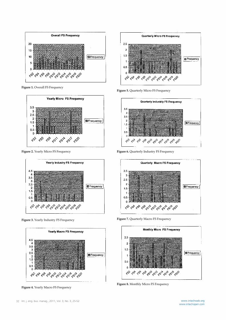
Figure 1. Overall FS Frequency

Figure 2. Yearly Micro FS Frequency

Figure 3. Yearly Industry FS Frequency

Figure 4. Yearly Macro FS Frequency

Figure 5. Quarterly Micro FS Frequency

Figure 6. Quarterly Industry FS Frequency

Figure 7. Quarterly Macro FS Frequency

Figure 8. Monthly Micro FS Frequency


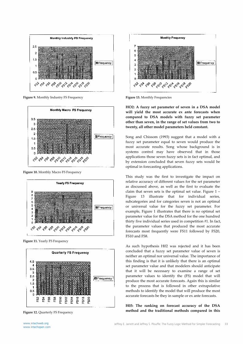
Figure 9. Monthly Industry FS Frequency

Figure 10. Monthly Macro FS Frequency

Figure 11. Yearly FS Frequency

Figure 12. Quarterly FS Frequency

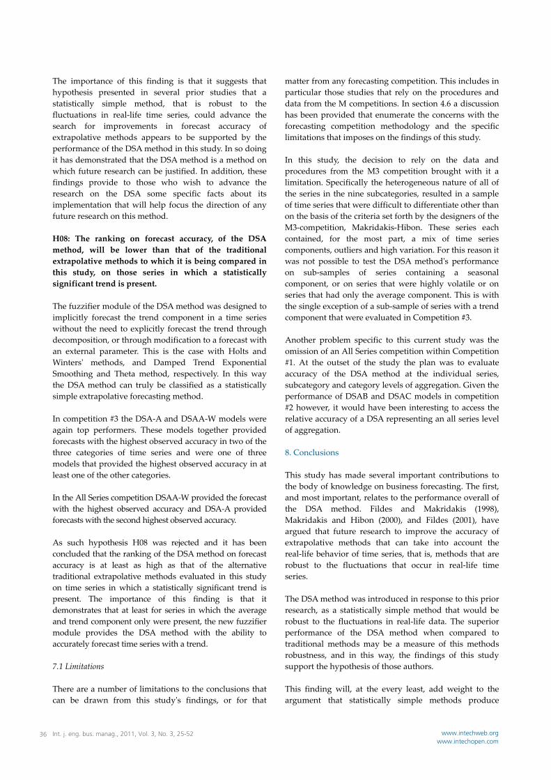
Figure 13. Monthly Frequencies HO2: A fuzzy set parameter of seven in a DSA model will yield the most accurate ex ante forecasts when compared to DSA models with fuzzy set parameter other than seven, in the range of set values from two to twenty, all other model parameters held constant. Song and Chissom (1993) suggest that a model with a fuzzy set parameter equal to seven would produce the most accurate results. Song whose background is in systems control may have observed that in those applications those seven fuzzy sets is in fact optimal, and by extension concluded that seven fuzzy sets would be optimal in forecasting applications. This study was the first to investigate the impact on relative accuracy of different values for the set parameter as discussed above, as well as the first to evaluate the claim that seven sets is the optimal set value. Figure 1 – Figure 13 illustrate that for individual series, subcategories and for categories seven is not an optimal or universal value for the fuzzy set parameter. For example, Figure 1 illustrates that there is no optimal set parameter value for the DSA method for the one hundred thirty five individual series used in competition #1. In fact, the parameter values that produced the most accurate forecasts most frequently were FS11 followed by FS20, FS10 and FS8. As such hypothesis H02 was rejected and it has been concluded that a fuzzy set parameter value of seven is neither an optimal nor universal value. The importance of this finding is that it is unlikely that there is an optimal set parameter value and that modelers should anticipate that it will be necessary to examine a range of set parameter values to identify the (FS) model that will produce the most accurate forecasts. Again this is similar to the process that is followed in other extrapolative methods to identify the model that will produce the most accurate forecasts be they in sample or ex ante forecasts. H03: The ranking on forecast accuracy of the DSA method and the traditional methods compared in this


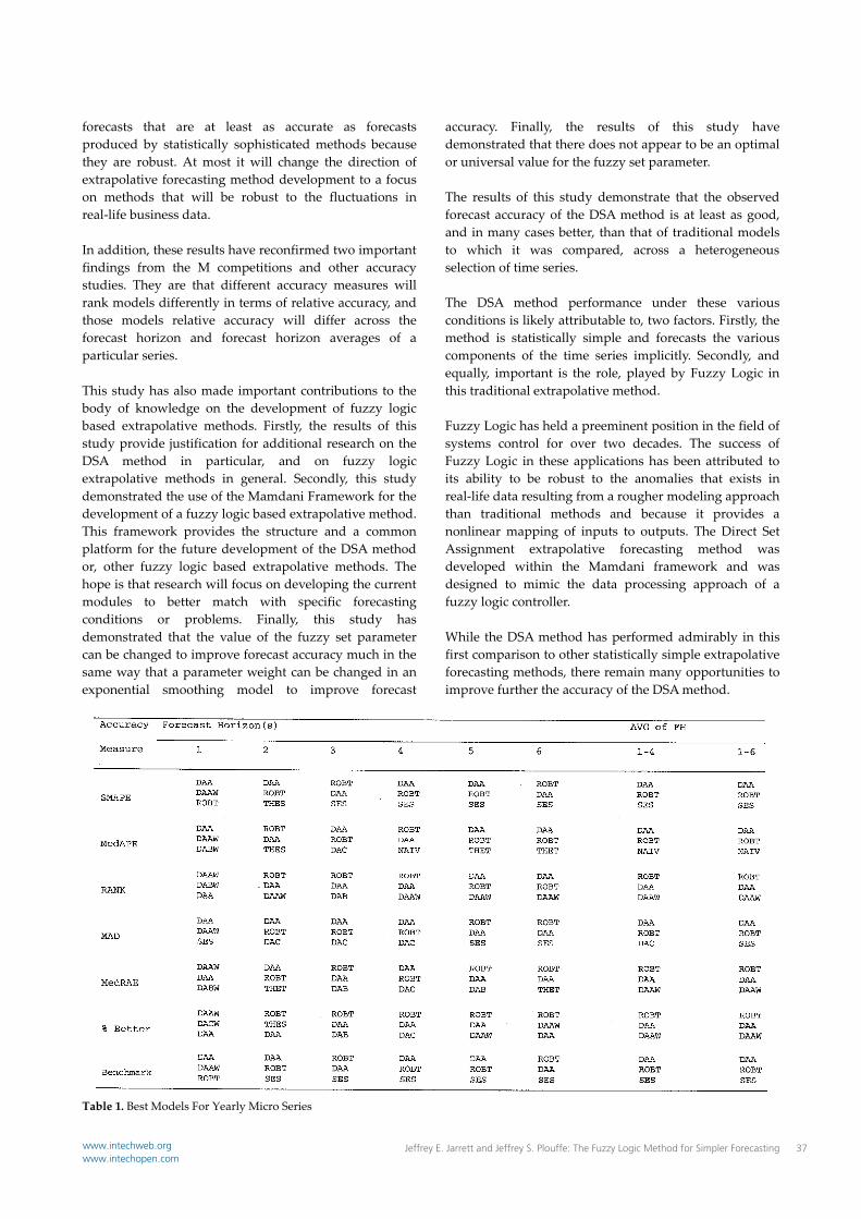
study will be the same for all accuracy measures considered. Table 1 – 16 for Competition #2 and 17 – 23 in Competition #3, excluding the summary tables; report the three models that provided the highest observed forecast accuracy, for subcategory, category and the all series levels of aggregation, for the seven accuracy measures, across the various forecast horizons. An examination of these tables reveals that the ranking of the three best performing methods in Competition #2 and Competition #3 differs, within a particular forecast horizon, for the seven measures of forecast accuracy. Similar results can be observed in the tables in Appendix C, containing the accuracy measures for each method. For example, in Table 2 for the average of all six forecast horizons, the order of methods on the basis of their sMAPE value is DAA, DAAW, and the order on the basis of Average Ranking is DAAW, DAA, and THET. As such hypothesis H03 was rejected and it has been concluded that the ranking of the forecast accuracy of various methods will be different for the various accuracy measured being used. The importance of this finding is that it reaffirms the findings of early studies including the M competitions and thus adds support to the existing body of knowledge on time series extrapolation. H04: The ranking on forecast accuracy of a combination of alternative forecasting methods will be lower than that of the specific forecasting methods being combined. In Table 17, the sMAPE values for the combination of three traditional methods, Single, Holt and Dampen, and their combination as well as for the DSA and Wintersʹ methods and their combination have been reported for various forecast horizons. Relative to the traditional methods and their combinations, the combination methods outperform Single and Holt’s exponential smoothing methods in their native form for all of the six sets of averaged forecast horizons. The combination however does not outperform Dampen Trend Exponential Smoothing for these same forecast horizons. For example, the sMAPE for S‐H‐D for the average of forecast horizons 1‐4 is 12.44 while the sMAPE for Dampen is 12.23. The other absolute differences are of approximately the same magnitude. Relative to the combination of the DSA and Winters Methods, the findings are mixed. For the DSAB‐W and DSAC‐W method the combination outperforms both of the DSA models and the Winters’ model in their native form. In the case of the DSAA‐W model the combination method outperforms the Wintersʹ method across all

forecast horizon averages; however the combined method does not outperform the DSAA model on any of the forecast horizon averages. For example the sMAPE for DSAA‐W for the average of forecast horizons 1‐4 is 10.63 while the sMAPE for the same forecast horizons is for the DSAA model is 10.00. Additionally, an examination of Table 21 indicates that the DSAA‐W model outperforms the DSAA and the Winters’ models on yearly data with a trend, while the DSAA model outperforms the DSAA‐W model on quarterly data with a trend. Further, in Table 23 DAA‐W outperforms all other models including the DSAA and Winterʹs models on all forty‐five series in which a statistically significant trend is present. As such hypothesis H04 was not rejected and it has been concluded that a combination of methods do not perform at least as well, in all settings, as do the methods that have been combined do, in their native form. This finding is disappointing in that this study has not reaffirmed a finding that has been reaffirmed in so many other accuracy studies. It may be that group difference testing could be used to resolve this disparity. H05: The ranking on forecast accuracy of the DSA method and the traditional methods compared in thus study does not depend on the length of the forecast horizon. Tables 1‐16 for Competition #2 and 17‐23 in Competition #3, excluding the summary tables, report the three models that provided the highest observed forecast accuracy, for subcategory, category and the all series levels of aggregation, for the seven accuracy measures, across the various forecast horizons. An examination of these tables reveals that the ranking of the three best performing methods in Competition #2 and Competition #3 differs, for a particular accuracy measure across forecast horizons, and the averages of those forecast horizons. Similar results can be observed in the tables, containing the accuracy measures for each method. For example, in Table 2 for the sMAPE accuracy measure, for forecast horizon 1, the three models with the highest observed accuracy are DAAW, DAA and THES and the three models for forecast horizon 3 are DAA, DAAW and DABW. Further, for the 1‐4 horizon average the models are ranked, DAAW, DAA and THES and for the 1‐6 horizon average the models are ranked, DAA, DAAW, and DABW. As such hypothesis H05 was rejected and it has been concluded that the ranking of the forecast accuracy of various methods will be different across different forecast horizons for a given measure of forecast accuracy. The importance of this finding is two fold. Firstly, it reaffirms the findings of early studies including the M competitions


and thus adds support to the existing body of knowledge on time series extrapolation. Secondly, it is important because it impacts on forecast method selection. The method that produces the most accurate forecast across the forecast horizons 1‐4 may well not be the method that produces the most accurate forecast over the forecast 1‐18. So, modelers should be certain that they select the model that will perform best for the forecast horizons of interest. H06: The ranking on forecast accuracy of the time series specific DSA model, will be less than or equal to the ranking on forecast accuracy of both the subcategory and category specific DSA models. H07: The ranking on forecast accuracy, of the DSA method, will be lower than that of the traditional extrapolative methods to which it is being compared in this study, by time series subcategory, time series category and for all of the time series evaluated in this study In competition #2 the goal was to establish the relative accuracy of the DSA‐A, DSA‐B, DSA‐C models, and eight traditional methods; a combination of traditional methods; and a combination of the DSA models and Winters Exponential Smoothing. The DSA‐A, DSA‐B and DSA‐C models were developed in competition #1 to help answer the question: Is there a fuzzy parameter value, for a data type and time interval subcategory, or a time interval category, that will yield more accurate results for those levels of aggregation, than it will for the series level of aggregation. Relative to the combination models, the traditional combination model was designated S‐H‐D and the fuzzy traditional combination models were designated DSAA‐W, DSAB‐W and DSAC‐W. Relative forecast accuracy was assessed at the subcategory, category and all series levels of aggregation in Competition #2. The results of this competition indicate that the forecasts represented by the DSA‐A model, when assessed at the subcategory, category and all series levels of aggregation, were more accurate, in the aggregate than were those represented by the DSA‐B and DSA‐C models. This finding is important but not necessarily surprising. This result suggests that the DSA method will produces the most accurate forecasts when it is used to produce ex ante forecast for the forecast horizons of an individual series, and less accurate forecasts will be obtained if the modeler selects a fuzzy set parameter for all series of a particular data type or time interval. Certainly, from the standpoint of the economy of the DSA method, it would have been preferable to have a single fuzzy parameter value that would produce the most accurate forecast for a subcategory or category of data. This would be particularly

true for manufacturing environments where forecasts for thousands of product components must be produced on a routine basis. This finding reinforces the findings in competition #1 that were used to test H01 and H02. In Competition #2 the DSAA model and its derivative, the DSAA‐W model dominated the competition. In the subcategory competition the DSAA model provided forecasts with the highest observed accuracy for five of the subcategories, while the DSAA‐W model provided forecasts with the highest observed accuracy for two for the subcategories. In total these two models provided forecasts with the highest observed accuracy for seven of nine subcategories. In the category competition the DSAA model and the DSAA‐W model each provided forecasts with the highest observed for one of the categories. In total, these two models provide the highest observed accuracy for two of three categories. In the All Series competition, the DSAA model provided forecasts with the highest observed accuracy for all one hundred thirty five, time series in this competition. The DSAA‐W method provided forecasts with the second highest observed accuracy. The Theta method that received such wide acclaim in the M3 competition was ranked third in the All Series competition. As such, hypotheses H06 and H07 were rejected. It was concluded relative to hypothesis H06 that the most accurate forecasts, for a large number of series in the aggregate, will be obtained by first obtaining the most accurate forecasts produced by the DSA method for the forecasts horizons of individual series. The importance of this finding is that it indicates to modelers that they should not assume that a particular fuzzy set parameter will produce the most accurate forecasts for a given data type but that they should first produce forecasts across the forecast horizon of each series in future studies of the DSA method. It was concluded relative to hypothesis H07 that the DSA‐A and DSAA‐W models produce forecasts that are in most cases more accurate, than those produced by the traditional extrapolative methods evaluated in this study. Remarkably, this conclusion holds across a broad range of time series that differ by, data types (micro, industry, macro); time origin, (yearly, quarterly, monthly); forecast horizon, (six, eight, eighteen); presence of a mix of time series components, (average trend and seasonal), and although it was not explicitly tested, training set length, (fourteen, seventeen, thirty‐six, forty‐one, fifty‐six, fifty‐one, fifty‐six, one‐hundred sixteen and one hundred twenty‐six). The exceptions to this list are Yearly‐Micro and Monthly‐Macro data.


The importance of this finding is that it suggests that hypothesis presented in several prior studies that a statistically simple method, that is robust to the fluctuations in real‐life time series, could advance the search for improvements in forecast accuracy of extrapolative methods appears to be supported by the performance of the DSA method in this study. In so doing it has demonstrated that the DSA method is a method on which future research can be justified. In addition, these findings provide to those who wish to advance the research on the DSA some specific facts about its implementation that will help focus the direction of any future research on this method. H08: The ranking on forecast accuracy, of the DSA method, will be lower than that of the traditional extrapolative methods to which it is being compared in this study, on those series in which a statistically significant trend is present. The fuzzifier module of the DSA method was designed to implicitly forecast the trend component in a time series without the need to explicitly forecast the trend through decomposition, or through modification to a forecast with an external parameter. This is the case with Holts and Wintersʹ methods, and Damped Trend Exponential Smoothing and Theta method, respectively. In this way the DSA method can truly be classified as a statistically simple extrapolative forecasting method. In competition #3 the DSA‐A and DSAA‐W models were again top performers. These models together provided forecasts with the highest observed accuracy in two of the three categories of time series and were one of three models that provided the highest observed accuracy in at least one of the other categories. In the All Series competition DSAA‐W provided the forecast with the highest observed accuracy and DSA‐A provided forecasts with the second highest observed accuracy. As such hypothesis H08 was rejected and it has been concluded that the ranking of the DSA method on forecast accuracy is at least as high as that of the alternative traditional extrapolative methods evaluated in this study on time series in which a statistically significant trend is present. The importance of this finding is that it demonstrates that at least for series in which the average and trend component only were present, the new fuzzifier module provides the DSA method with the ability to accurately forecast time series with a trend. 7.1 Limitations There are a number of limitations to the conclusions that can be drawn from this studyʹs findings, or for that

matter from any forecasting competition. This includes in particular those studies that rely on the procedures and data from the M competitions. In section 4.6 a discussion has been provided that enumerate the concerns with the forecasting competition methodology and the specific limitations that imposes on the findings of this study. In this study, the decision to rely on the data and procedures from the M3 competition brought with it a limitation. Specifically the heterogeneous nature of all of the series in the nine subcategories, resulted in a sample of time series that were difficult to differentiate other than on the basis of the criteria set forth by the designers of the M3‐competition, Makridakis‐Hibon. These series each contained, for the most part, a mix of time series components, outliers and high variation. For this reason it was not possible to test the DSA methodʹs performance on sub‐samples of series containing a seasonal component, or on series that were highly volatile or on series that had only the average component. This is with the single exception of a sub‐sample of series with a trend component that were evaluated in Competition #3. Another problem specific to this current study was the omission of an All Series competition within Competition #1. At the outset of the study the plan was to evaluate accuracy of the DSA method at the individual series, subcategory and category levels of aggregation. Given the performance of DSAB and DSAC models in competition #2 however, it would have been interesting to access the relative accuracy of a DSA representing an all series level of aggregation. 8. Conclusions This study has made several important contributions to the body of knowledge on business forecasting. The first, and most important, relates to the performance overall of the DSA method. Fildes and Makridakis (1998), Makridakis and Hibon (2000), and Fildes (2001), have argued that future research to improve the accuracy of extrapolative methods that can take into account the real‐life behavior of time series, that is, methods that are robust to the fluctuations that occur in real‐life time series. The DSA method was introduced in response to this prior research, as a statistically simple method that would be robust to the fluctuations in real‐life data. The superior performance of the DSA method when compared to traditional methods may be a measure of this methods robustness, and in this way, the findings of this study support the hypothesis of those authors. This finding will, at the every least, add weight to the argument that statistically simple methods produce


forecasts that are at least as accurate as forecasts produced by statistically sophisticated methods because they are robust. At most it will change the direction of extrapolative forecasting method development to a focus on methods that will be robust to the fluctuations in real‐life business data. In addition, these results have reconfirmed two important findings from the M competitions and other accuracy studies. They are that different accuracy measures will rank models differently in terms of relative accuracy, and those models relative accuracy will differ across the forecast horizon and forecast horizon averages of a particular series. This study has also made important contributions to the body of knowledge on the development of fuzzy logic based extrapolative methods. Firstly, the results of this study provide justification for additional research on the DSA method in particular, and on fuzzy logic extrapolative methods in general. Secondly, this study demonstrated the use of the Mamdani Framework for the development of a fuzzy logic based extrapolative method. This framework provides the structure and a common platform for the future development of the DSA method or, other fuzzy logic based extrapolative methods. The hope is that research will focus on developing the current modules to better match with specific forecasting conditions or problems. Finally, this study has demonstrated that the value of the fuzzy set parameter can be changed to improve forecast accuracy much in the same way that a parameter weight can be changed in an exponential smoothing model to improve forecast

accuracy. Finally, the results of this study have demonstrated that there does not appear to be an optimal or universal value for the fuzzy set parameter. The results of this study demonstrate that the observed forecast accuracy of the DSA method is at least as good, and in many cases better, than that of traditional models to which it was compared, across a heterogeneous selection of time series. The DSA method performance under these various conditions is likely attributable to, two factors. Firstly, the method is statistically simple and forecasts the various components of the time series implicitly. Secondly, and equally, important is the role, played by Fuzzy Logic in this traditional extrapolative method. Fuzzy Logic has held a preeminent position in the field of systems control for over two decades. The success of Fuzzy Logic in these applications has been attributed to its ability to be robust to the anomalies that exists in real‐life data resulting from a rougher modeling approach than traditional methods and because it provides a nonlinear mapping of inputs to outputs. The Direct Set Assignment extrapolative forecasting method was developed within the Mamdani framework and was designed to mimic the data processing approach of a fuzzy logic controller. While the DSA method has performed admirably in this first comparison to other statistically simple extrapolative forecasting methods, there remain many opportunities to improve further the accuracy of the DSA method.

Table 1. Best Models For Yearly Micro Series


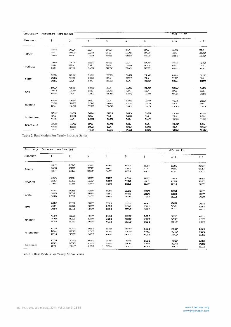
Table 2. Best Models For Yearly Industry Series

Table 3. Best Models For Yearly Micro Series


Table 4. Best Models For Quarterly Micro Series

Table 5. Best Models For Quarterly Industry Series


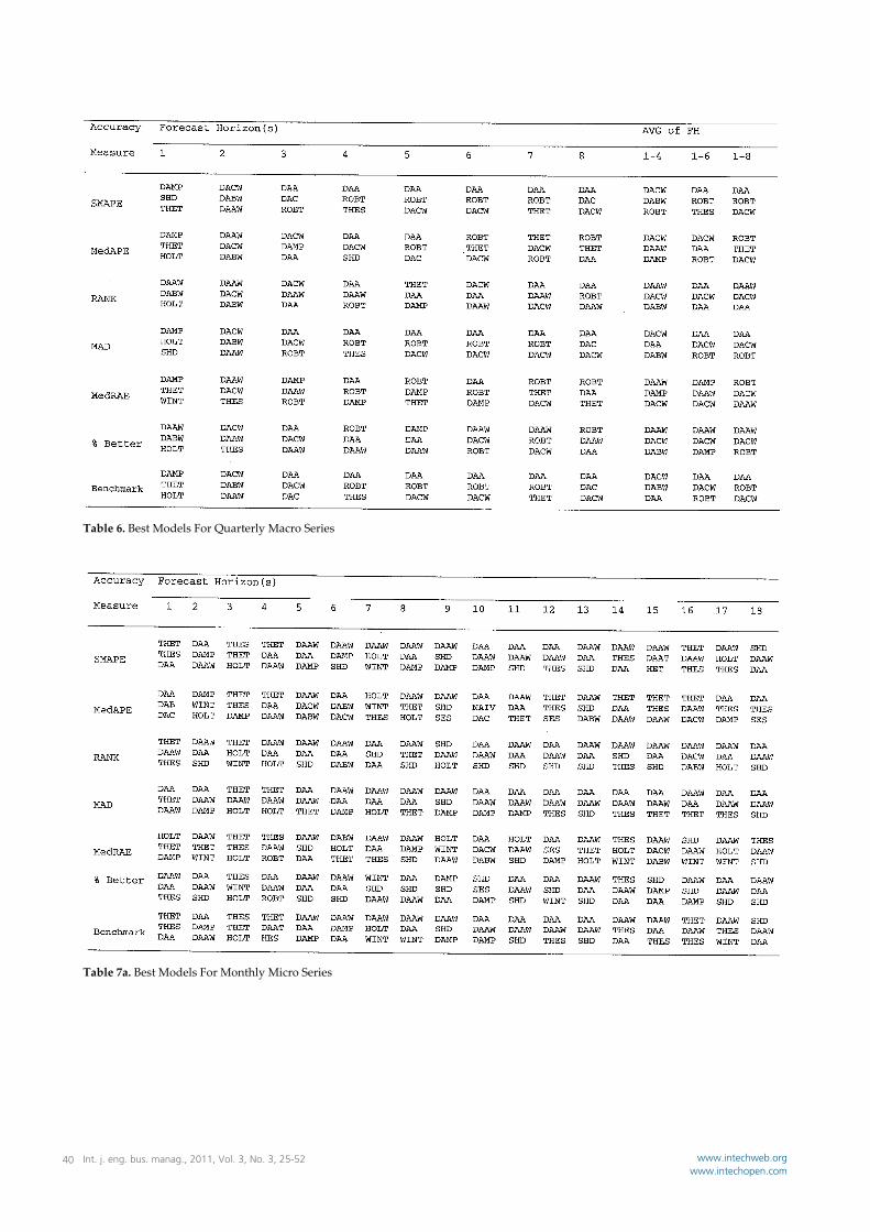
Table 6. Best Models For Quarterly Macro Series

Table 7a. Best Models For Monthly Micro Series


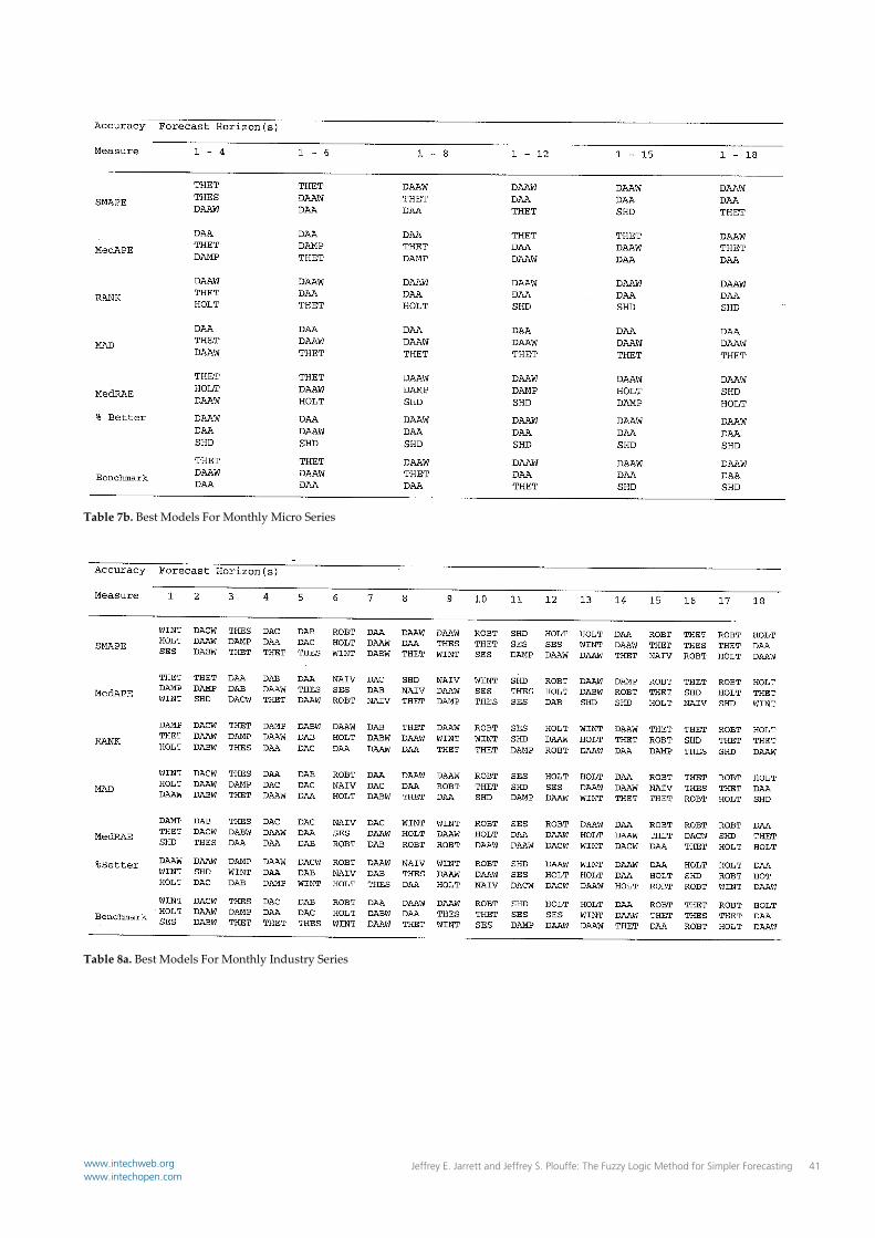
Table 7b. Best Models For Monthly Micro Series

Table 8a. Best Models For Monthly Industry Series


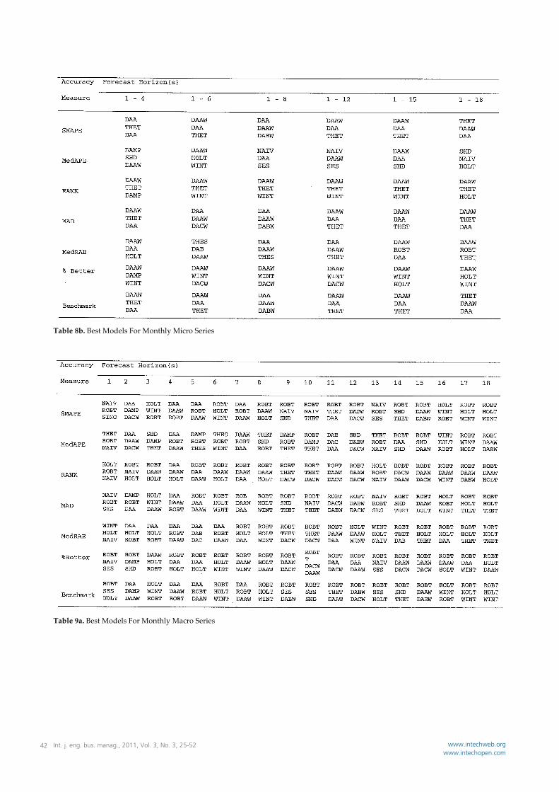
Table 8b. Best Models For Monthly Micro Series

Table 9a. Best Models For Monthly Macro Series


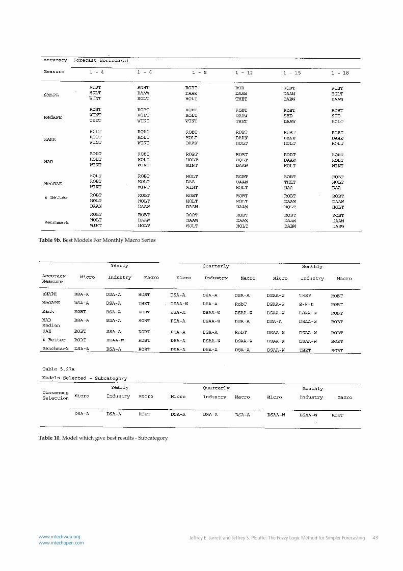
Table 9b. Best Models For Monthly Macro Series

Table 10. Model which give best results ‐ Subcategory


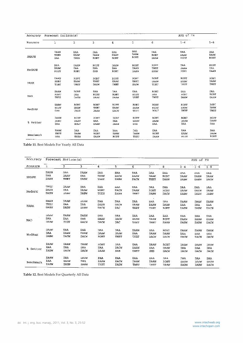
Table 11. Best Models For Yearly All Data

Table 12. Best Models For Quarterly All Data


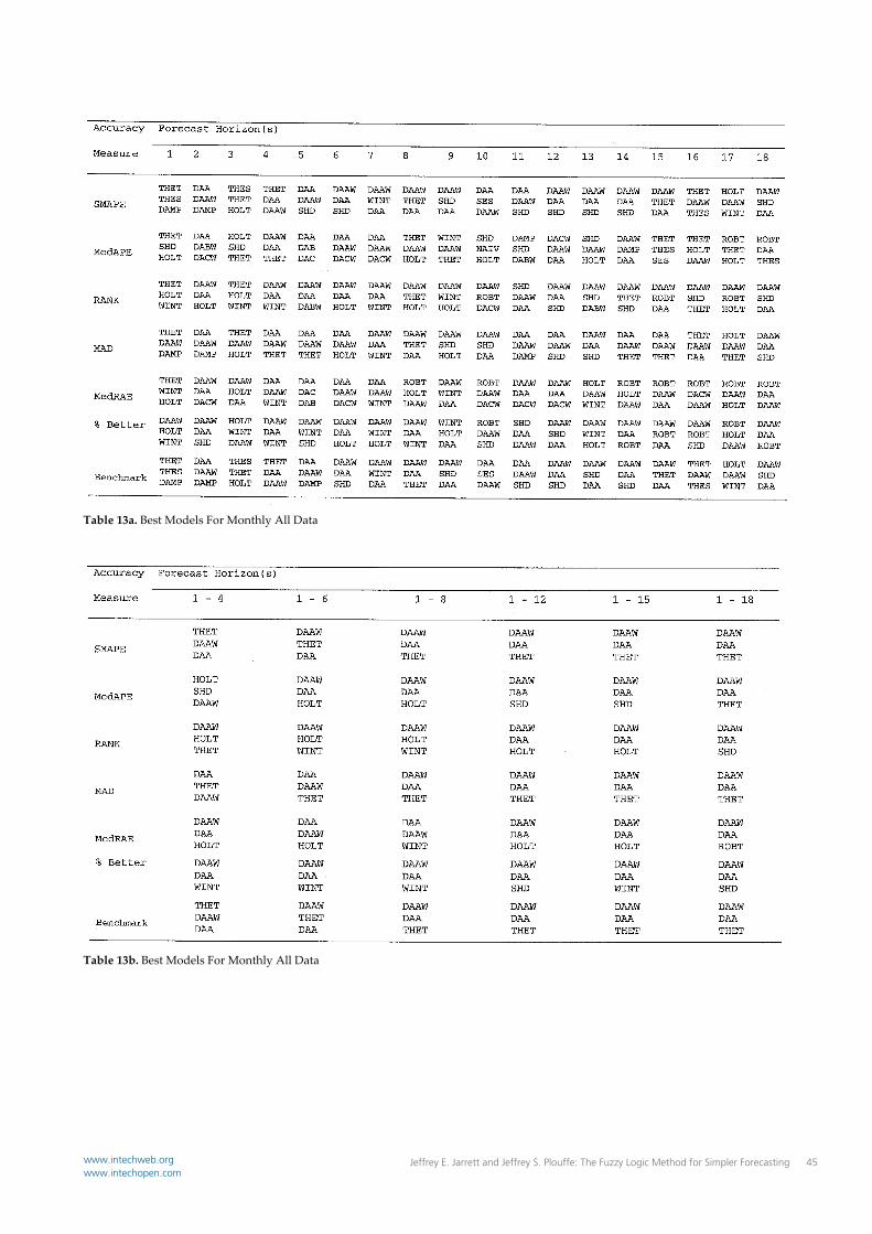
Table 13a. Best Models For Monthly All Data

Table 13b. Best Models For Monthly All Data


Table 14. Model which give best results ‐ category

Table 15a. Best Models For Overall Data


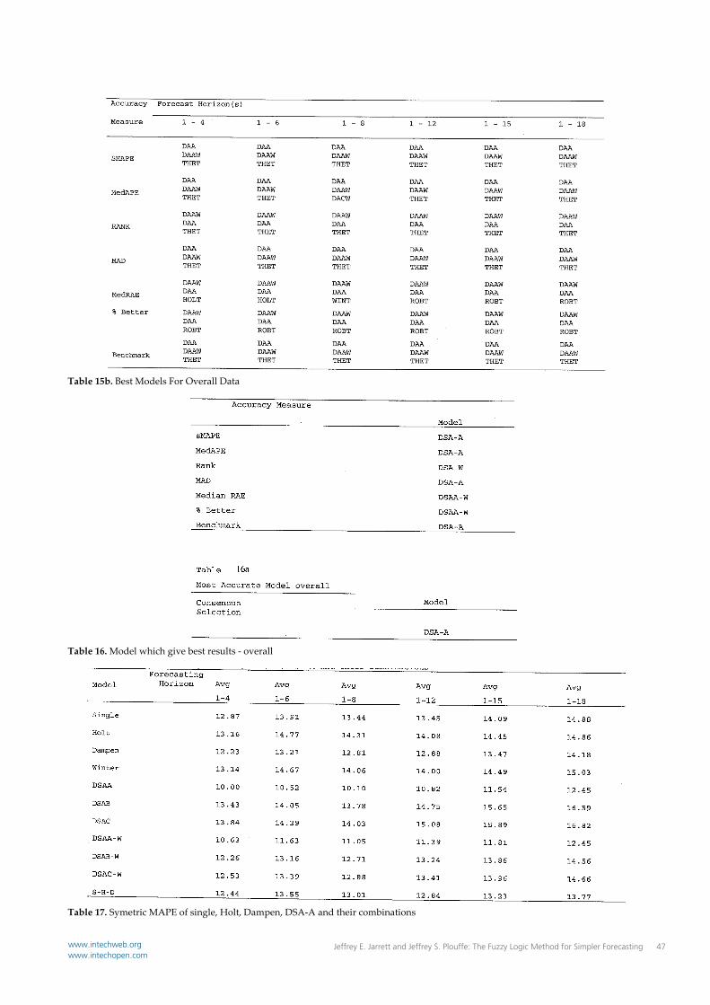
Table 15b. Best Models For Overall Data

Table 16. Model which give best results ‐ overall

Table 17. Symetric MAPE of single, Holt, Dampen, DSA‐A and their combinations


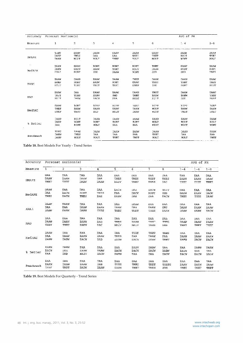
Table 18. Best Models For Yearly ‐ Trend Series

Table 19. Best Models For Quarterly ‐ Trend Series


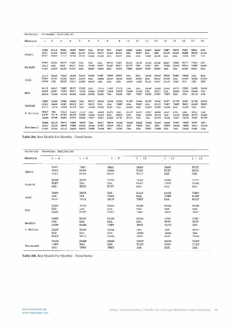
Table 20a. Best Models For Monthly ‐ Trend Series

Table 20b. Best Models For Monthly ‐ Trend Series


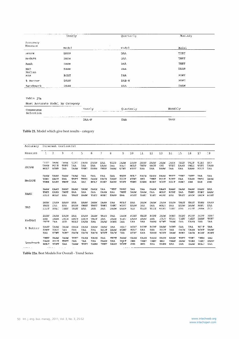
Table 21. Model which give best results ‐ category

Table 22a. Best Models For Overall ‐ Trend Series


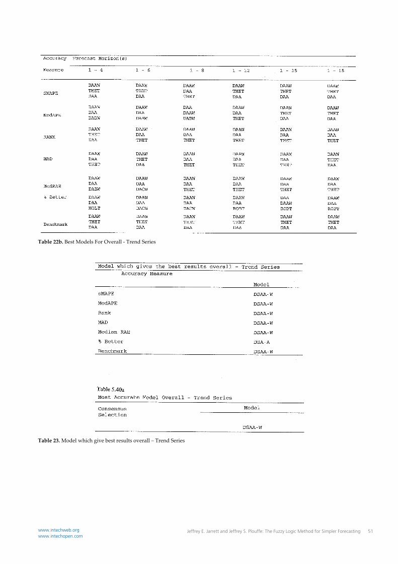
Table 22b. Best Models For Overall ‐ Trend Series

Table 23. Model which give best results overall – Trend Series


9. References [1] Armstrong, S.J., & Collopy, F. (1992A). Error Measures

for Generalizing about Forecasting Methods. International Journal of Forecasting, 8(2), 69‐80.

[2] Armstrong, S.J., & Collopy, F. (1992B). Casual Forces: Structuring Knowledge for Time Series Extrapolation. Journal of Forecasting, 12, 103‐115.

[3] Brandon, C. Jarrett, J.E. & Khumuwala, S. B. (1983) Revising Forecasts of Accounting Earnings: A Comparison with the Box‐Jenkins Method, Management Science, 29, 256‐264.

[4] Brandon, C. and Jarrett, J.E. (1979) Revising Earnings per Share Forecasts: An Empirical Test, Management Science, 25, 211‐220.

[5] Brandon, C. Jarrett, J.E. & Khumuwala, S. B. (1986) Comparing Forecast Accuracy for Exponential Models of Earnings‐Per‐Share Data for Financial Decision Making, Decision Sciences, 17, 186‐194.

[6] Chen, S. (1996). Forecasting Enrollments Based on Fuzzy Time Series. Fuzzy Sets and Systems, 81, 311‐319.

[7] Clements, M.P. & Hendry, D.F. (1989) Explaining the Results of the M3 Forecasting Competition. International Journal of Forecasting, 17, 537‐584.

[8] Collett, D., & Lewis, T. (1976). The Subjective Nature of Outlier Rejection Procedures. Applied Statistics, 25(3), 228‐237.

[9] Elton, Edwin, J., and Gruber, Martin, J. (1972). Earnings Estimates and the Accuracy of Expectational Data. Management Science, 18(8).

[10] Fildes, R., Hibon, M., Makridakis, S., & Meade, N. (1998). Generalizing About Univariate Forecasting Methods: Further Empirical Evidence. International Journal of Forecasting, 14, 339‐358.

[11] Fildes, R. (2001). Beyond forecasting competitions. International Journal of Forecasting, 17(4), 537‐584.

[12] Jarrett, J.E., (1990) Forecasting Seasonal Time Series of Corporate Earnings:A Note, Decision Sciences, 21, 4, 888‐893.

[13] Jarrett, J.E. and Khumuwala, S.B. (1987), A Study of Forecast Error and Covariant Time Series to Improve Forecasting for Financial Decision Making, Managerial Finance, 13, 2, 20‐27.

[14] Jarrett, J.E., & Plouffe, J. S. (2006). Forecasting Occupancy Levels: A Problem for Management Forecasters, Journal of Business and Management, 12, 1, 59‐69.

[15] Koehler, A. B., & Murphee, E. S. (1988). A Comparison of the Results Form State Space Forecasting for the Makridakis Competition. International Journal of Forecasting.

[16] Lusk, E. J., & Neves, J. S. (1984). A Comparative ARIMA Analysis of the 111 Series of the Makridakis Competition. Journal of Forecasting, 329‐332.

[17] Makridakis, S., & Hibon, M. (1979). Accuracy of Forecasting: An Empirical Investigation (with discussion). Journal of the Royal Statistical Society; A, 142, 97‐145.

[18] Makridakis, S., Chatfield, C., Hibon, M., Lawrence, M., Mils, T., Ord, K., Simmons, L. F. (1993). The M2‐Competition: A Real‐time Judgmentally based Forecasting Study. International Journal of Forecasting, 9(1), 5‐23.

[19] Makridakis, S., & Hibon, M. (2000). The M3‐Competition: results, Conclusions and implications. International Journal of Forecasting, 16, 451‐476.

[20] Mukaidono, Masao (2002). Fuzzy Logic for Beginners. Singapore, New Jersey, London, Hong Kong: World Scientific Publishing Co.

[21] Newbold, P., & Granger, C.W.J. (1974). Experience With Forecasting Univariate Time Series and The Combination of Statistical Society; A, 137, 131‐165.

[22] Ried, D.J. (1972). A Comparison of Forecasting Techniques on Econometric Time Series; in Bramson, M. J., Helps, I.G. & Watson‐Gandy, J.A.C.C., (Eds.), Forecasting in Action, Birmingham: OR Society.

[23] Song, Q., & Chissom, B.S. (1993). Forecasting Enrollments with Fuzzy Time Series: Part I. Fuzzy Sets and Systems, 54(1), 1‐9.

[24] Song Q., & Chissom, B.S. (1994). Forecasting Enrollments with Fuzzy Time Series: Part 2. Fuzzy Sets and Systems. 62(1), 1‐8.


the fuzzy logic method for simpler forecastingcdn.intechweb.org/pdfs/17984.pdf · the fuzzy logic...

Documents