the geometric tools of hilbert spaces
TRANSCRIPT

'
&
$
%
The Geometric Tools of Hilbert Spaces
Erlendur Karlsson
February 2009
c©2009 by Erlendur KarlssonAll rights reserved. No part of this manuscript is to bereproduced without the writen consent of the author.

Contents
1 Orientation 1
2 Definition of Inner Product Spaces 2
3 Examples of Inner Product Spaces 3
4 Basic Objects and Their Properties 54.1 Vectors and Tuples . . . . . . . . . . . . . . . . . . . . . . . . . . . . . . . 54.2 Sequences . . . . . . . . . . . . . . . . . . . . . . . . . . . . . . . . . . . . 74.3 Subspaces . . . . . . . . . . . . . . . . . . . . . . . . . . . . . . . . . . . . 8
5 Inner Product and Norm Properties 9
6 The Projection Operator 11
7 Orthogonalizations of Subspace Sequences 167.1 Different Orthogonalizations of Sy
t,p . . . . . . . . . . . . . . . . . . . . . . 167.1.1 The Backward Orthogonalization of Sy
t,p . . . . . . . . . . . . . . . 167.1.2 The Forward Orthogonalization of Sy
t,p . . . . . . . . . . . . . . . . 167.1.3 The Eigenorthogonalization of Sy
t,p . . . . . . . . . . . . . . . . . . 177.2 Different Orthogonalizations of SZ
t,p . . . . . . . . . . . . . . . . . . . . . . 187.2.1 The Backward Block Orthogonalization of SZ
t,p . . . . . . . . . . . 187.2.2 The Forward Block Orthogonalization of SZ
t,p . . . . . . . . . . . . 19
8 Procedures for Orthogonalizing Syt,p and SZ
t,p 198.1 The Gram–Schmidt Orthogonalization Procedure . . . . . . . . . . . . . . 198.2 The Schur Orthogonalization Procedure . . . . . . . . . . . . . . . . . . . 20
9 The Dynamic Levinson Orthogonalization Procedure 229.1 The Basic Levinson Orthogonalization Procedure . . . . . . . . . . . . . . 22
9.1.1 The Basic Levinson Orthogonalization Procedure for Syt,p . . . . . 23
9.1.2 The Basic Block Levinson Orthogonalization Procedure for SZt,p . . 25
9.2 Relation Between The Projection Coefficients of Different Basis . . . . . . 279.2.1 Relation Between Direct Form and Lattice Realizations on Sy
t,i . . 279.2.2 Relation Between Direct Form and Lattice Realizations on SZ
t,i . . 299.3 Evaluation of Inner Products . . . . . . . . . . . . . . . . . . . . . . . . . 30
9.3.1 Lattice Inner Products for Syt,p . . . . . . . . . . . . . . . . . . . . 30
9.3.2 Lattice Inner Products for SZt,p . . . . . . . . . . . . . . . . . . . . 30
9.4 The Complete Levinson Orthogonalization Procedure . . . . . . . . . . . 31
i

1
1 Orientation
Our goal in this course is to study and develop model based methods for adaptive sys-tems. Although it is possible to do this without explicit use of the geometric toolsof Hilbert spaces, there are great advantages to be gained from a geometric formula-tion. These are largely derived from our familiarity with Euclidean geometry and inparticular with the concepts of orthogonality and orthogonal projections. The intuitiongained from Euclidean geometry will serve as our guide to constructive development ofcomplicated algorithms and will often help us to understand and interpret complicatedalgebraic results in a geometrically obvious way. These notes are devoted to a study ofthose aspects of Hilbert space theory which are needed for the constructive geometricdevelopment. For the reader who wishes to go deeper into the theory of Hilbert spaceswe can recommend the books by Kreyszig [1] and Mate [2].
In two– and three–dimensional Euclidean spaces we worked with geometric objects suchas vectors and subspaces. We studied various geometric properties of these objects suchas the norm of a vector, the angle between two vectors and the orthogonality of onevector with respect to another. We also learned about geometrical operations on theseobjects such as projecting a vector onto a subspace and orthogonalizing a subspace.These powerful geometric concepts and tools were also intuitive, natural and easy tograsp as we could actually see them or visualize them in two– and three–dimensionaldrawings.
These geometric concepts and tools were easily extended to the n–dimensional Euclideanspace (n > 3), through the scalar product. Even here simple two– and three–dimensionaldrawings can be useful in illustrating or visualizing geometric phenomenon.
One proof of how essetial the geometric machinery is in mathematics is that it can also beextended to infinite–dimensional vector spaces, this time using an extesion of the scalarproduct, namely the inner product. Going to an infinite–dimensional vector space makesthings more complicated. The lack of a finite basis is one such complication that cre-ates difficulties in applications. Fortunately, many infinite–dimensional normed spacescontain an infinite sequence of vectors called a fundamental sequence, such that everyvector in the space can be approximated to any accuracy with a linear combination ofvectors belonging to the fundamental sequence. Such infinite dimensional spaces occurfrequently in engineering and one can work with those in pretty much the same wayone works with finite dimensional spaces. Another complication is that of completeness.When an inner product space is not complete, it has holes, meaning that there existelements of finite norm that are not in the inner product space but can be approximatedto any desired accuracy by an element of the inner product space. The good news is thatall incomplete inner product spaces can be constructively extended to complete innerproduct spaces. A Hilbert space is a complete inner product space.

2 2 DEFINITION OF INNER PRODUCT SPACES
In these notes we go through the following moments:
2 Definition of Inner Product Spaces3 Examples of Inner Product Spaces4 Basic Objects and Their Properties5 Inner Product and Norm Properties6 The Projection Operator7 Orthogonalizations of the Subspaces Sy
t,p and SZt,p
8 Procedures for Orthogonalizing Syt,p and SZ
t,p
9 The Dynamic Levinson Orthogonalization Procedure
2 Definition of Inner Product Spaces
Definition 2-1 An Inner Product SpaceAn inner product space H, 〈·, ·〉 is a vector space H equipped with an inner product〈·, ·〉, which is a mapping from H×H onto the scalar field of H (real or complex).
For all vectors x, y and z in H and scalar α, the inner product satisfies the four axioms
IP1 : 〈x + y, z〉 = 〈x, z〉+ 〈y, z〉IP2 : 〈αx,y〉 = α 〈x,y〉IP3 : 〈x,y〉 = 〈y,x〉∗
IP4 : 〈x,x〉 ≥ 0〈x,x〉 = 0⇔ x = 0.
An inner product on H defines a norm on H given by
||x|| =√〈x,x〉
and a metric on H given by
d(x,y) = ||x − y|| =√〈x − y,x − y〉.
Remark 2-1 Think EuclideanThe inner product is a natural generalization of the scalar product of two vectors in ann–dimensional Euclidean space. Since many of the properties of the Euclidean spacecarry over to inner product spaces, it will be helpful to keep the Euclidean space in mindin all that follows.
3
3 Examples of Inner Product Spaces
Example 3-1 The Euclidean space Cn, 〈x,y〉 =∑n
i=1 xiy∗i
The n–dimensional vector space over the complex field, Cn, with the inner productbetween two vectors
x =
x1...xn
and y =
y1...yn
defined by
〈x,y〉 =n∑
i=1
xiy∗i
where y∗i is the complex conjugation of yi, is an inner product space. This gives thenorm
||x|| = 〈x,x〉1/2 =
√√√√ n∑i=1
|xi|2
and the Euclidean metric
d(x,y) = ||x − y|| = 〈x − y,x − y〉1/2 =
√√√√ n∑i=1
|xi − yi|2
Example 3-2 The space of square summable sequencesl2, 〈x,y〉 =
∑∞i=1 xiy
∗i
The vector space of square summable sequences with the inner product between the twosequemces x = xi and y = yi defined by
〈x,y〉 =∞∑i=1
xiy∗i
where y∗i is the complex conjugation of yi, is an inner product space. This gives thenorm
||x|| = 〈x,x〉1/2 =
√√√√ ∞∑i=1
xix∗i
and the metric
d(x,y) = ||x− y|| = 〈x− y,x− y〉1/2 =
√√√√ ∞∑i=1
|xi − yi|2
Example 3-3 The space of square integrable functionsL2, 〈f,g〉 =
∫fg∗
The vector space of square integrable functions defined on the interval [a, b], with theinner product defined by
〈f,g〉 =∫ b
af(τ)g∗(τ)dτ
4 3 EXAMPLES OF INNER PRODUCT SPACES
where g∗(τ) is the complex conjugation of g(τ), is an inner product space. This givesthe norm
||f|| = 〈f, f〉1/2 =
√∫ b
af(τ)f∗(τ)dτ
and the metric
d(f,g) = ||f − g|| = 〈f − g, f − g〉1/2 =
√∫ b
a|f(τ)− g(τ)|2dτ
Example 3-4 The continuous functions over [0, 1], C([0, 1]), 〈f,g〉 =∫
fg∗
The vector space of continuous functions defined on the interval [0, 1], with the innerproduct defined by
〈f,g〉 =∫ 1
0f(τ)g∗(τ)dτ
where g∗(τ) is the complex conjugation of g(τ), is an inner product space. This givesthe norm
||f|| = 〈f, f〉1/2 =
√∫ 1
0f(τ)f∗(τ)dτ
and the metric
d(f,g) = ||f − g|| = 〈f − g, f − g〉1/2 =
√∫ 1
0|f(τ)− g(τ)|2dτ
Example 3-5 Random variables with finite second order moments,L2(Ω,B, P ), 〈x,y〉 = E(xy∗) =
∫Ω x(ω)y∗(ω)dP (w)
The space of random variables with finite 2nd moments, L2(Ω,B, P ), with the innerproduct defined by
〈x,y〉 = E(xy∗) =∫
Ωx(ω)y∗(ω)dP (w)
where E is the expectation operator, is an inner product space. Here a random variabledenotes the equivalence class of random variables on (Ω,B, P ), where y is equivalent tox if E|x − y|2 = 0.
This gives the norm
||x|| = 〈x,x〉1/2 =√E|x|2
and the metric
d(x,y) = ||x − y|| = 〈x − y,x − y〉1/2 =√E|x − y|2.

5
4 Basic Objects and Their Properties
Here we will get acquainted with the main geometrical objects of the space and theirproperties. We begin by looking at the most basic objects vectors and tuples. We thenproceed with sequences and subspaces.
4.1 Vectors and Tuples
Definition 4.1-1 VectorThe basic element of a vector space is called a vector. In the case of the n–dimensionalEuclidean vector space this is the standard n–dimensional vector, in the space of squaresummable sequences this is a square summable sequence and in the space of square in-tegrable functions this is a square integrable function.
Definition 4.1-2 TupleAn n–tuple is an ordered set of n elements. An n–tuple made up of the n vectorsx1,x2, . . . ,xn is denoted by x1,x2, . . . ,xn. We will mostly be using n–tuples of vec-tors and parameter coefficients (scalars).
Definition 4.1-3 Norm of a VectorThe norm of a vector x, denoted by ‖x‖, is a measure of its size. More precisely it is amapping from the vector space onto the positive reals, which for all vectors x and y inH and scalar α satisfies the following axioms:
N1 : ‖x‖ ≥ 0‖x‖ = 0⇔ x = 0
N2 : ‖x + y‖ ≤ ‖x‖+ ‖y‖N3 : ‖αx‖ = |α|‖x‖
In an inner product space the norm is always derived from the inner product as follows:
||x|| = 〈x,x〉1/2
It is an easy exercise to show that the above definition satisfies the norm axioms.
Definition 4.1-4 OrthogonalityTwo vectors x and y of an inner product space H are said to be orthogonal if
〈x,y〉 = 0,
and we write x ⊥ y.
An n–tuple of vectors, x1,x2, . . .xn, is said to be orthogonal if
〈xn,xm〉 = 0 for all n 6= m.
Definition 4.1-5 Angle Between Two VectorsIn a real inner product space the angle θ between the two vectors x and y is defined bythe formula
cos(θ) =〈x,y〉||x||||y||
.

6 4 BASIC OBJECTS AND THEIR PROPERTIES
Definition 4.1-6 Linear Combination of Vectors and Tuples of VectorsA linear combination of vectors x1,x2, . . . ,xn is an expression of the form
α(1)x1 + α(2)x2 + . . .+ α(n)xn =n∑
i=1
α(i)xi
where the coefficients α(1), α(2), . . . α(n) are any scalars. Sometimes we will also wantto express this sum in the form of a matrix multiplication
n∑i=1
α(i)xi = x1,x2, . . . ,xn
α(1)...
α(n)
︸ ︷︷ ︸
α
= x1,x2, . . . ,xnα,
where we consider the n–tuple x1,x2, . . . ,xn as being a form of a row vector multi-plying the column vector α.
Similarly a linear combination of m–tuples X1,X2, . . . ,Xn where Xk is an m–tuple ofvectors xk,1,xk,2, . . . ,xk,m is actually a linear combination of the vectors x1,1, . . . ,x1,m,x2,1, . . . ,x2,m, . . . ,xn,1, . . . ,xn,m given by
n∑i=1
m∑j=1
α(i, j)xi,j
which can be expressed in matrix notation as
n∑i=1
m∑j=1
α(i, j)xi,j =n∑
i=1
xi,1, . . . ,xi,m
α(i, 1)...
α(i,m)
︸ ︷︷ ︸
αi
=n∑
i=1
Xiαi
= X1, . . . ,Xn
α1...αn
.
Still another linear combination is when an m-tuple Z = z1, z2, . . . , zm is formed fromlinear combinations of the n-tuple X = x1,x2, . . . ,xn, where
zi =n∑
j=1
αi(j)xj = x1,x2, . . . ,xn
αi(1)...
αi(n)
︸ ︷︷ ︸
αi
= x1,x2, . . . ,xnαi.
We can then write
Z = z1, z2, . . . , zm
= x1,x2, . . . ,xn (α1, . . . ,αm)︸ ︷︷ ︸α
= Xα

4.2 Sequences 7
Definition 4.1-7 Linear Independence and DependenceThe set of vectors x1,x2, . . .xn is said to be linearly independent if the only n–tuple ofscalars α1, α2, . . . αn that makes
α1x1 + α2x2 + . . .+ αnxn = 0 (4.1)
is the all zero n–tuple with α1 = α2 = . . . = αn = 0. The set of vectors is said to belinearly dependent if it is not linearly independent. In that case there exists an n–tupleof scalars different from the all zero n–tuple, that satisfies equation (4.1).
Definition 4.1-8 Inner Product Between Tuples of VectorsGiven the p–tuple of vectors X = x1, . . . ,xp and the q–tuple of vectors Y = y1, . . . ,yq,the inner product between the two is defined as the matrix
〈X,Y〉 =
〈x1,y1〉 . . . 〈xp,y1〉...
. . ....
〈x1,yq〉 . . . 〈xp,yq〉
This inner product between tuples of vectors is often used to simplify notaion.
For the vector–tuples X, Y and Z and the coefficient matrices α and β the followingproperties hold:
IP1 : 〈X + Y,Z〉 = 〈X,Z〉+ 〈Y,Z〉IP2 : 〈Xα,Y〉 = 〈X,Y〉α
〈X,Yβ〉 = βH 〈X,Y〉IP3 : 〈X,Y〉 = 〈Y,X〉H
IP4 : 〈X,X〉 ≥ 0〈X,X〉 = 0⇔ X = 0.
4.2 Sequences
Definition 4.2-1 SequenceA sequence is an infinite ordered set of elements. We will denote sequences of vectors byxn or xn : n = 1, 2, . . ..
Definition 4.2-2 Convergence of SequencesA sequence xn in a normed space X is said to converge to x if x ∈ X and
limn→∞
||xn − x|| = 0
Definition 4.2-3 Cauchy SequenceA sequence xn in a normed space X is said to be Cauchy if for every ε > 0 there is apositive integer N such that
||xn − xm|| < ε for all m,n > N.

8 4 BASIC OBJECTS AND THEIR PROPERTIES
4.3 Subspaces
Definition 4.3-1 Linear SubspaceA subset S of H is called a linear subspace if for all x, y ∈ S and all scalars α, β in thescalar field of H, it holds that αx + βy ∈ S. S is therefore a linear space over the samefield of scalars. S is said to be a proper subspace of H if S 6= H.
Definition 4.3-2 Finite and Infinite Dimensional Vector SpacesA vector space H is said to be finite dimensional if there is a positive integer n suchthat H contains a linearly independent set of n vectors whereas any set of n+ 1 or morevectors is linearly dependent. n is called the dimension of H, written dimH = n. Bydefinition, H = 0 is finite dimensional and dimH = 0. If H is not finite dimensional,it is said to be infinite dimensional.
Definition 4.3-3 Span and Set of Spanning VectorsFor any nonempty subsetM⊂ H the set S of all linear combinations of vectors inM iscalled the span of M, written S = SpM. Obviously S is a subspace of H and we saythat S is spanned or generated byM. We also say thatM is the set of spanning vectorsof S.
Definition 4.3-4 Basis for Vector SpacesFor an n–dimensional vector space S, an n–tuple of linearly independent vectors in Sis called a basis for S. If x1,x2, . . .xn is a basis for S, every x ∈ S has a uniquerepresentation as a linear combination of the basis vectors
x = α1x1 + α2x2 + . . .+ αnxn.
This idea of a basis can be extended to infinite–dimensional vector spaces with the socalled Schauder basis. Not all infinite–dimensional vector spaces have a Schauder basis,however, the ones of interest for engineers do.
For an infinite–dimensional vector space H, a sequence of vectors in H, xn, is aSchauder basis for H, if for every x ∈ H there is a unique sequence of scalars αn suchthat
limn→∞
||x−n∑
k=1
αkxk|| = 0
The sum∑∞
k=1 αkxk is then called the expansion of x with respect to xn, and we write
x =∞∑
k=1
αkxk
Proposition 4.3-1 Tuples of Vectors Spanning the Same SubspaceGiven an n–dimensional subspace S = SpX, where X is an n–tuple of the linearlyindependent vectors x1, . . . ,xn, then X is a basis for S and each vector in S is uniquelywritten as a linear combination of the vectors in X. If we now pick the n–vectorsy1, . . . ,yn in S, where
yk =n∑
i=1
αk(i)xi
9
= x1, . . . ,xn
αk(1)...
αk(n)
︸ ︷︷ ︸
αk
= Xαk,
then Y = y1, . . . ,yn is also a basis for S if the parameter vectors αk for k = 1, 2, . . . , nare linearly independent. A convenient way of expressing this linear mapping from X toY is to write
Y = Xα,
where α is the matrix of parameter vectors
α =
α1(1) . . . αn(1)...
. . ....
α1(n) . . . αn(n)
= (α1, . . . ,αn) .
Here it helps to look at Xα as the matrix multiplication between the n–tuple X (con-sidered as a row vector) and the matrix α. Then yk can be seen as Xαk =
∑ni=1 αk(i)xi.
When the parameter vectors in α are linearly independent, α has full rank and is in-vertible. Then it is also possible to write X as a linear mapping from Y
X = Yα−1,
where α−1 is the inverse matrix of α.
Definition 4.3-5 Orthogonality
A vector y is said to be orthogonal to a finite subspace Sn = Spx1, . . . ,xn if y isorthogonal to all the spanning vectors of Sn, x1 . . . ,xn, and we write y ⊥ Sn.
Definition 4.3-6 Completeness
In some inner product spaces there exist sequences that converge to a vector that is nota member of the inner product space. It is for example easy to construct a sequenceof continous functions that converges to a discontinous function. These types of innerproduct spaces have ”holes” and are said to be incomplete. Inner product spaces whereevery Cauchy sequence converges to a member of the inner product space are said to becomplete. A Hilbert space is a complete inner product space.
5 Inner Product and Norm Properties
Theorem 5-1 The Cauchy–Schwartz inequalityIn an inner product space H there holds:
| 〈x,y〉 | ≤ ‖x‖ ‖y‖ for all x, y ∈ H. (5.1)
Equality holds in (5.1) if and only if x and y are linearly dependent or either of the twois zero.

10 6 THE PROJECTION OPERATOR
Proof: The equality obviously holds if x = 0 or y = 0. If x 6= 0 and y 6= 0 then for anyscalar λ we have
0 ≤ 〈x− λy,x− λy〉= 〈x,x〉+ |λ|2 〈y,y〉 − 〈λy,x〉 − 〈x, λy〉 (5.2)= 〈x,x〉+ |λ|2 〈y,y〉 − 〈λy,x〉 − 〈λy,x〉∗
= 〈x,x〉+ |λ|2 〈y,y〉 − 2Re(λ 〈y,x〉).
For λ = 〈x,y〉〈y,y〉 we have
0 ≤ 〈x,x〉 − | 〈x,y〉 |2
〈y,y〉
and the Cauchy–Schwartz inequality is obtained by suitable rearrangement. From theproperties of the inner product it follows at once that if x = λy, then the equality holds.Conversely, if the equality holds, then either x = 0, y = 0, or else it follows from (5.2)that there exists a λ such that
x− λy = 0,
i.e. x and y are linearly dependent.
Proposition 5-1 The triangle inequalityIn an inner product space H there holds:
‖x + y‖2 ≤ (‖x‖ + ‖y‖)2 for all x, y ∈ H. (5.3)
Equality holds in (5.3) if and only if x and y are linearly dependent or either of the twois zero.
Proof: This follows directly from the Cauchy–Schwartz inequality
‖x + y‖2 = 〈x + y,x + y〉= 〈x,x〉+ 2Re(〈x,y〉) + 〈y,y〉≤ ‖x‖2 + 2| 〈x,y〉 |+ ‖y‖2
≤ ‖x‖2 + 2‖x‖ ‖y‖+ ‖y‖2
= (‖x‖+ ‖y‖)2.
Proposition 5-2 The parallelogram equalityIn an inner product space H there holds:
‖x + y‖2 + ‖x − y‖2 = 2(‖x‖2 + ‖y‖2) for all x, y ∈ H. (5.4)
Proof: There holds:
‖x ± y‖2 = ‖x‖2 ± 2Re(〈x,y〉) + ‖y‖2
By adding we get the parallelogram equality.
11
6
-
1
6
-
H
y
y −PS(y) ⊥ S
s = PS(y)
S
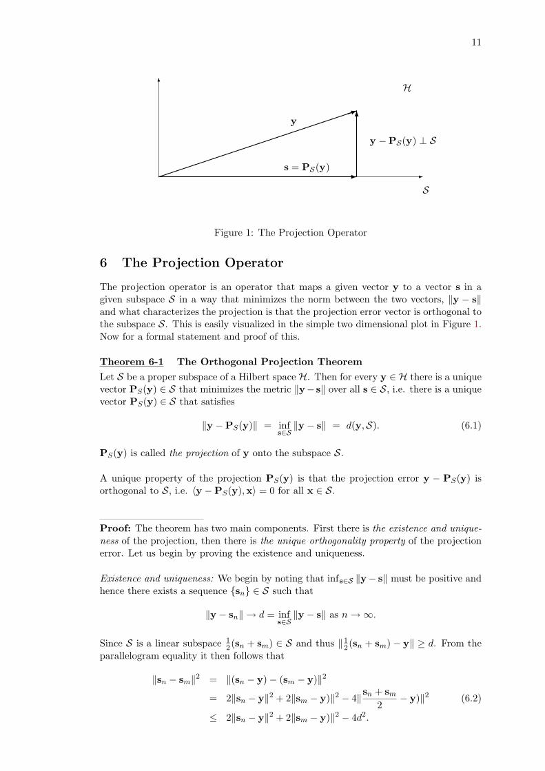
Figure 1: The Projection Operator
6 The Projection Operator
The projection operator is an operator that maps a given vector y to a vector s in agiven subspace S in a way that minimizes the norm between the two vectors, ‖y − s‖and what characterizes the projection is that the projection error vector is orthogonal tothe subspace S. This is easily visualized in the simple two dimensional plot in Figure 1.Now for a formal statement and proof of this.
Theorem 6-1 The Orthogonal Projection Theorem
Let S be a proper subspace of a Hilbert space H. Then for every y ∈ H there is a uniquevector PS(y) ∈ S that minimizes the metric ‖y− s‖ over all s ∈ S, i.e. there is a uniquevector PS(y) ∈ S that satisfies
‖y −PS(y)‖ = infs∈S‖y − s‖ = d(y,S). (6.1)
PS(y) is called the projection of y onto the subspace S.
A unique property of the projection PS(y) is that the projection error y − PS(y) isorthogonal to S, i.e. 〈y −PS(y),x〉 = 0 for all x ∈ S.
Proof: The theorem has two main components. First there is the existence and unique-ness of the projection, then there is the unique orthogonality property of the projectionerror. Let us begin by proving the existence and uniqueness.
Existence and uniqueness: We begin by noting that infs∈S ‖y− s‖ must be positive andhence there exists a sequence sn ∈ S such that
‖y − sn‖ → d = infs∈S‖y − s‖ as n→∞.
Since S is a linear subspace 12(sn + sm) ∈ S and thus ‖1
2(sn + sm) − y‖ ≥ d. From theparallelogram equality it then follows that
‖sn − sm‖2 = ‖(sn − y)− (sm − y)‖2
= 2‖sn − y‖2 + 2‖sm − y)‖2 − 4‖sn + sm
2− y)‖2 (6.2)
≤ 2‖sn − y‖2 + 2‖sm − y)‖2 − 4d2.

12 6 THE PROJECTION OPERATOR
The right-hand side of (6.2) tends to zero as m,n → ∞ and thus sn is a Cauchysequence. Since H is complete and S is closed
sn → PS(y) ∈ S and ‖y −PS(y)‖ = d.
If we substitute in the expression (6.2) sn = z and sm = PS(y) we obtain z = PS(y),from which the uniqueness follows.
Unique orthogonality property of the projection error: What we need to show is thatz = PS(y) if and only if y−z is orthogonal to every s ∈ S, or in other words if and onlyif y− z ∈ S⊥. We begin by showing that e = y−PS(y) ⊥ S. Let w ∈ S with ‖w‖ = 1.Then for any scalar λ, PS(y) + λw ∈ S. The minimal property of PS(y) then impliesthat for any scalar λ
‖e‖2 = ‖y −PS(y)‖2 ≤ ‖y −PS(y)− λw‖2
= ‖e− λw‖2 = 〈e− λw, e− λw〉 . (6.3)
That is0 ≤ −λ 〈w, e〉 − λ∗ 〈e,w〉+ |λ|2 for all scalars λ.
Choosing λ = 〈e,w〉 then gives 0 ≤ −| 〈e,w〉 |2. Consequently 〈e,w〉 = 0 for all w ∈ Sof unit norm, and it follows this orthogonal relation holds for all w ∈ S.
Next we show that if 〈y − z,w〉 = 0 for some z ∈ S and all w ∈ S, then z = PS(y).Let z ∈ S and assume that 〈y − z,w〉 = 0 for all w ∈ S. Then for z ∈ S we have thaty − z ∈ S and that x− y ⊥ y − z. Consequently we have that
‖x− z‖2 = ‖(x− y) + (y − z)‖2 = ‖(x− y)‖2 + ‖(y − z)‖2.
As a result,‖x− z‖2 ≥ ‖(x− y)‖2
for all z ∈ S, with equality only if y − z = 0, as required.
Corollary 6-1 Projecting a Vector onto a Finite Subspace
Given a finite subspace spanned by the linearly independent vectors x1, . . . ,xn, S =Spx1, . . . ,xn, the projection of a vector y onto S is given by
PS(y) =n∑
i=1
α(i)xi
= x1, . . . ,xn
α(1)...
α(n)
︸ ︷︷ ︸
α
where the projection coefficient vector α satisfies the normal equation 〈x1,x1〉 . . . 〈xn,x1〉...
. . ....
〈x1,xn〉 . . . 〈xn,xn〉
α(1)
...α(n)
=
〈y,x1〉...
〈y,xn〉
.Defining the n–tuple of vectors X = x1, . . . ,xn and using the definition of an innerproduct between tuples of vectors the normal equation can be written in the morecompact form
〈X,X〉α = 〈y,X〉

13
For a 1-dim subspace S = Spx, the projection of y onto S simply becomes
PS(y) = αx,
whereα =
〈y,x〉〈x,x〉
=〈y,x〉||x||2
.
Proof: The normal equation comes directly from the orthogonality property of theprojection error, namely
y −PSn(y) ⊥ x1, . . . ,xn
⇓〈y −PSn(y),xq〉 = 0 for q = 1, . . . , n
⇓〈y,xq〉 = 〈PSn(y),xq〉 for q = 1, . . . , n
⇓n∑
i=1
α(i) 〈xi,xq〉 = 〈y,xq〉 for q = 1, . . . , n
Writing this up in matrix format gives the above normal equation.
Corollary 6-2 Projecting a Tuple of Vectors onto a Finite Subspace
Given a finite subspace spanned by the linearly independent n–tuple X = x1, . . . ,xn,S = SpX = Spx1, . . . ,xn, we have seen in Corollary 6-1 that the projection of avector yk onto S is given by
PS(yk) =n∑
i=1
αk(i)xi
= x1, . . . ,xn
αk(1)...
αk(n)
︸ ︷︷ ︸
αk
where the projection coefficient vector αk satisfies the normal equation 〈x1,x1〉 . . . 〈xn,x1〉...
. . ....
〈x1,xn〉 . . . 〈xn,xn〉
αk(1)
...αk(n)
=
〈yk,x1〉...
〈yk,xn〉
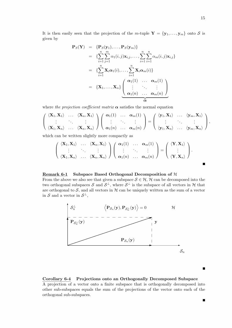
.It is then easily seen that the projection of the m-tuple Y = y1, . . . ,ym onto S isgiven by
PS(Y) = PS(y1), . . . ,PS(ym)
= n∑
i=1
α1(i)xi, . . . ,n∑
i=1
αm(i)xi
= x1, . . . ,xn
α1(1) . . . αm(1)...
. . ....
α1(n) . . . αm(n)
︸ ︷︷ ︸
α

14 6 THE PROJECTION OPERATOR
where the projection coefficient matrix α satisfies the normal equation 〈x1,x1〉 . . . 〈xn,x1〉...
. . ....
〈x1,xn〉 . . . 〈xn,xn〉
α1(1) . . . αm(1)
.... . .
...α1(n) . . . αm(n)
=
〈y1,x1〉 . . . 〈ym,x1〉...
. . ....
〈y1,xn〉 . . . 〈ym,xn〉
,which is more compactly writen as
〈X,X〉α = 〈Y,X〉 .
Corollary 6-3 Projecting an m–tuple Y onto the span of the m–tuplesX1, . . . ,Xn
Given a finite subspace S spanned by the linearly independent set ofm–tuples X1, . . . ,Xn
with Xi = xi,1, . . . ,xi,m we have that
S = SpX1,X2, . . . ,Xn= Spx1,1, . . . ,x1,m,x2,1, . . . ,x2,m, . . . ,xn,1, . . . ,xn,m
Then from Corollary 6-1 we have that the projection of a vector yk onto S is given by
PS(yk) =n∑
i=1
m∑j=1
αk(i, j)xi,j
= x1,1, . . . ,x1,m,x2,1, . . . ,x2,m, . . . ,xn,1, . . . ,xn,m
αk(1, 1)...
αk(1,m)
αk(1)
αk(2, 1)...
αk(2,m)
αk(2)
...
αk(n, 1)...
αk(n,m)
αk(n)
︸ ︷︷ ︸
αk
where the projection coefficient vector αk satisfies the normal equation
〈x1,1,x1,1〉 . . . 〈x1,m,x1,1〉 〈xn,1,x1,1〉 . . . 〈xn,m,x1,1〉...
. . .... . . .
.... . .
...〈x1,1,x1,m〉 . . . 〈x1,m,x1,m〉 〈xn,1,x1,m〉 . . . 〈xn,m,x1,m〉
.... . .
...
〈x1,1,xn,1〉 . . . 〈x1,m,xn,1〉 〈xn,1,xn,1〉 . . . 〈xn,m,xn,1〉...
. . .... . . .
.... . .
...〈x1,1,xn,m〉 . . . 〈x1,m,xn,m〉 〈xn,1,xn,m〉 . . . 〈xn,m,xn,m〉
αk(1, 1)...
αk(1,m)
...
αk(n, 1)...
αk(n,m)
=
〈yk,x1,1〉...
〈yk,x1,m〉
...
〈yk,xn,1〉...
〈yk,xn,m〉
,
which again is written in more compact for as 〈X1,X1〉 . . . 〈Xn,X1〉...
. . ....
〈X1,Xn〉 . . . 〈Xn,Xn〉
αk(1)
...αk(n)
=
〈yk,X1〉...
〈yk,Xn〉
.
15
It is then easily seen that the projection of the m-tuple Y = y1, . . . ,ym onto S isgiven by
PS(Y) = PS(y1), . . . ,PS(ym)
= n∑
i=1
m∑j=1
α1(i, j)xi,j , . . . ,n∑
i=1
n∑i=1
αm(i, j)xi,j
= n∑
i=1
Xiα1(i), . . . ,n∑
i=1
Xiαm(i)
= X1, . . . ,Xn
α1(1) . . . αm(1)...
. . ....
α1(n) . . . αm(n)
︸ ︷︷ ︸
α
where the projection coefficient matrix α satisfies the normal equation 〈X1,X1〉 . . . 〈Xn,X1〉...
. . ....
〈X1,Xn〉 . . . 〈Xn,Xn〉
α1(1) . . . αm(1)
.... . .
...α1(n) . . . αm(n)
=
〈y1,X1〉 . . . 〈ym,X1〉...
. . ....
〈y1,Xn〉 . . . 〈ym,Xn〉
,which can be written slightly more compactly as 〈X1,X1〉 . . . 〈Xn,X1〉
.... . .
...〈X1,Xn〉 . . . 〈Xn,Xn〉
α1(1) . . . αm(1)
.... . .
...α1(n) . . . αm(n)
=
〈Y,X1〉...
〈Y,Xn〉
.
Remark 6-1 Subspace Based Orthogonal Decomposition of HFrom the above we also see that given a subspace S ∈ H, H can be decomposed into thetwo orthogonal subspaces S and S⊥, where S⊥ is the subspace of all vectors in H thatare orthogonal to S, and all vectors in H can be uniquely written as the sum of a vectorin S and a vector in S⊥,
6
-
1
6
-
S⊥n H
y
⟨PSn(y),PS⊥n (y)
⟩= 0
PS⊥n (y)
PSn(y)
Sn
Corollary 6-4 Projections onto an Orthogonally Decomposed SubspaceA projection of a vector onto a finite subspace that is orthogonally decomposed intoother sub-subspaces equals the sum of the projections of the vector onto each of theorthogonal sub-subspaces.

16 7 ORTHOGONALIZATIONS OF SUBSPACE SEQUENCES
7 Orthogonalizations of Subspace Sequences
One of the most important subspaces that shows up in adaptive systems is the subspace
Syt,p = Spyt−1,yt−2, . . . ,yt−p (7.1)
where yt∞t=0 is a sequence of vectors yt in some Hilbert space H, which can be eitherdeterministic or stochastic. This kind of subspace comes up when modelling single inputsingle output (SISO) moving average (MA) and autoregressive (AR) systems.
Another important subspace is
SZt,p = Sp Zt−1,Zt−2, . . . ,Zt−p (7.2)
where Zt∞t=0 is a sequence of q-tuples of vectors, Zt = zt,1, . . . , zt,q, in some Hilbertspace H. This subspaces can be seen as a block version of the former and comes upwhen modelling single input single output ARX systems, certain types of time–varyingsystems and multi input multi output (MIMO) systems.
The adaptive algorithms we will be studying in this course are based on orthogonaliza-tions of these two subspaces. Let us therefore take a closer look at the main orthogonal-izations.
7.1 Different Orthogonalizations of Syt,p
There exist infinitely many orthogonalizations of Syt,p, but there are three commonly
used orthogonalizations that are of interest in adaptive systems. These are the backwardorthogonalization, the forward orthogonalization and the eigenorthogonalization.
7.1.1 The Backward Orthogonalization of Syt,p
The most common orthogonalization of Syt,p = Spyt−1,yt−2, . . . ,yt−p is the backward
orthogonalization where the latest spanning vector yt−1 is choosen as the first basisvector and one then moves backwards in time to orthogonalize the rest of the vectorswith respect to the vectors in their future domain as shown in Figure 2 below.
yt−1, . . . ,yt−i︸ ︷︷ ︸ ← yt−(i+1)︸ ︷︷ ︸ yt−(i+2), . . . ,yt−p
Syt,i bt,i = yt−(i+1) −Pt,i(yt−(i+1))
Figure 2: Backward Orthogonalization of Syt,p = Spyt−1,yt−2, . . . ,yt−p
The vectors bt,i are called the backward projection errors and with this orthogonalizationwe can write Sy
t,p asSy
t,p = Spbt,0,bt,1, . . . ,bt,p−1.
7.1.2 The Forward Orthogonalization of Syt,p
The forward orthogonalization of Syt,p is a dual orthogonalization to the backward or-
thogonalization. There the oldest spanning vector yt−p is chosen as the first basis vectorand one then moves forward in time to orthogonalize the rest of the vectors with respectto the vectors in their past domain. The orthogonalization will then be the one shownbelow.

7.1 Different Orthogonalizations of Syt,p 17
yt−1, . . . ,yt−(p−i−1) yt−(p−i)︸ ︷︷ ︸ → yt−(p−i+1), . . . ,yt−p︸ ︷︷ ︸yt−(p−i) −Pt−(p−i),i(yt−(p−i)) = et−(p−i),i Sy
t−(p−i),i
Figure 3: Forward Orthogonalization of Syt,p = Spyt−1,yt−2, . . . ,yt−p.
The vectors et−(p−i),i are called the forward projection errors and with this orthogonal-ization we can write Sy
t,p as
Syt,p = Spet−1,p−1, . . . , et−(p−1),1, et−p,0.
7.1.3 The Eigenorthogonalization of Syt,p
The eigenorthogonalization is the most decoupled orthogonalization there is, in that itorthogonalizes Sy
t,p in such a way that the projection coefficient vectors describing theorthogonal basis vectors in terms of the given spanning vectors also form an orthogonalset of vectors. The name eigenorthogonalization comes from the close coupling of thisorthogonalization to the eigendecomposition of the related Gram–matrix. This is prob-ably too abstract to follow, so let us go through this more slowly.
As we mentioned in the beginning of this section, there are infinitely many ways oforthogonalizing the subspace
Syt,p = Spyt−1,yt−2,yt−3, . . . ,yt−p.
An interesting question is, therefore, if there exists an orthogonalization of Syt,p where
the orthogonal basis vectors are given by
xt,k =p∑
i=1
αk(i)yt−i for k = 1, 2, . . . , p
and the parameter vectors describing the basis vectors in terms of the given spanningvectors
αk =
αk(1)αk(2)...αk(p)
also form an orthogonal basis in Cp?
The answer turnes out to be yes. To obtain a unique solution the parameter vectorbasis α1, . . . ,αp is made orthonormal (orthogonal and unit norm). We call the or-thogonalization the eigenorthogonalization because the parameter vectors αk satisfy theeigenequation
〈Yt,Yt〉αk = ||xt,k||2αk, (7.3)
where Yt is the p–tuple yt−1,yt−2, . . . ,yt−p.
To see this we first need the relation between 〈Xt,Xt〉 and 〈Yt,Yt〉. The result thenfollows from looking at the inner product 〈xt,k,Yt〉. Now as Xt = Yt (α1, . . . ,αp) =YtA we have that
〈Xt,Xt〉 =
‖xt,1‖2 0. . .
0 ‖xt,p‖2

18 7 ORTHOGONALIZATIONS OF SUBSPACE SEQUENCES
= 〈YtA,YtA〉= AH 〈Yt,Yt〉A
and
〈Yt,Yt〉 = A−H 〈Xt,Xt〉A−1.
Then as the parameter vector basis α1, . . . ,αp is orthonormal we have that AHA = I,i.e. A−1 = AH and A−H = A, which again gives
〈Yt,Yt〉 = A 〈Xt,Xt〉AH .
With these two relations between 〈Xt,Xt〉 and 〈Yt,Yt〉 we can move onto the innerproduct 〈xt,k,Yt〉 :
〈xt,k,Yt〉 = 〈Ytαk,Yt〉= 〈Yt,Yt〉αk
= A 〈Xt,Xt〉AHαk︸ ︷︷ ︸ek
= A‖xt,k‖2ek
= ‖xt,k‖2αk
which gives us the eigenequation (7.3).
Assuming that the spanning vectors yt−1, . . . ,yt−p are linearly independent, 〈Yt,Yt〉is a positive definite matrix, which will have real and positive eigenvalues and orthog-onal eigenvectors. We see here that the eigenvalues will be the squared norms of theeigenorthogonal basis vectors and the parameter vectors describing those basis vectorsin terms of the given spanning vectors will be the eigenvectors. From this we see thatthe eigenorthogonalization actually exists and that it can be evaluated with the use ofthe eigendecomposition of the Gram-matrix 〈Yt,Yt〉 or the singular decomposition ofYt.
7.2 Different Orthogonalizations of SZt,p
The difference between SZt,p and Sy
t,p is that SZt,p is the span of the n q–tuples Zt−1, . . . ,Zt−p,
while Syt,p is the span of the n vectors yt−1, . . . ,yt−p. Instead of fully orthogonalizing
SZt,p into nq one dimensional subspaces, we can orthogonalize it into n q–dimensional
subspaces in pretty much the same way we orthogonalized Syt,p, working with q–tuples
instead of vectors. Let us look at the backward block orthogonalization and the forwardblock orthogonalization of SZ
t,p.
7.2.1 The Backward Block Orthogonalization of SZt,p
The most common orthogonalization of SZt,p = SpZt−1,Zt−2, . . . ,Zt−p is the backward
block orthogonalization where the latest spanning tuple Zt−1 is choosen as the first basistuple and one then moves backwards in time to orthogonalize the rest of the vectortuples with respect to the vector tuples in their future domain as shown in Figure 4.The vector tuples Bt,i are called the backward projection errors and with this orthogo-nalization we can write SZ
t,p as
SZt,p = SpBt,0,Bt,1, . . . ,Bt,p−1.

19
Zt−1, . . . ,Zt−i︸ ︷︷ ︸ ← Zt−(i+1)︸ ︷︷ ︸ Zt−(i+2), . . . ,Zt−p
SZt,i Bt,i = Zt−(i+1) −Pt,i(Zt−(i+1))
Figure 4: Backward Block Orthogonalization of SZt,p = SpZt−1,Zt−2, . . . ,Zt−p
7.2.2 The Forward Block Orthogonalization of SZt,p
The forward block orthogonalization of SZt,p is a dual orthogonalization to the backward
orthogonalization. There the oldest spanning vector-tuple Zt−p is chosen as the firstbasis tuple and one then moves forward in time to orthogonalize the rest of the tupleswith respect to the ones in their past domain. The orthogonalization will then be theone shown in Figure 5.
Zt−1, . . . ,Zt−(p−i−1) Zt−(p−i)︸ ︷︷ ︸ → Zt−(p−i+1), . . . ,Zt−p︸ ︷︷ ︸Zt−(p−i) −Pt−(p−i),i(Zt−(p−i)) = Et−(p−i),i SZ
t−(p−i),i
Figure 5: Forward Block Orthogonalization of SZt,p = SpZt−1,Zt−2, . . . ,Zt−p.
The vector tuples Et−(p−i),i are called the forward projection errors and with this or-thogonalization we can write SZ
t,p as
SZt,p = SpEt−1,p−1, . . . ,Et−(p−1),1,Et−p,0.
8 Procedures for Orthogonalizing Syt,p and SZt,p
We have often been confronted with the problem of orthogonalizing a given subspace,and are well familiar with the Gram-Schmidt orthogonalization procedure. A familiarexample is the subspace of n-th order polynomials defined on the interval [−1, 1], wherethe inner product between the functions f and g is defined by 〈f ,g〉 =
∫ 1−1 f(t)g(t)dt.
This space is spanned by the functions f0, f1, . . . , fn, where fk(t) = tk for t ∈ [−1, 1] andk = 0, 1, . . . , n. Orthogonalizing this subspace with the Gram-Schmidt orthogonalizationprocedure results in the well known Legendre polynomial basis functions. In this sectionwe will study that and the related Schur–orthogonalization procedure for orthogonalizingthe subspaces Sy
t,p and SZt,p.
8.1 The Gram–Schmidt Orthogonalization Procedure
The Gram–Schmidt orthogonalization procedure is an efficent orthogonalization proce-dure for orthogonalizations such as the backward and forward orthogonalizations. Themain idea behind the procedure is that the subspace is orthogonalized in an order recur-siva manner so that the subspaces beeing projected onto are always orthogonal or blockorthogonal. This allows each projection to be evaluated in terms of orthogonal or blockorthogonal basis vectors, thus making the procedure relatively efficient.
The orthogonalization precedure for the backward orthogonalization of Syt,p is shown
below, where Pt,k(x) denotes the projection of the vector x onto Syt,k:

20 8 PROCEDURES FOR ORTHOGONALIZING SYT,P AND SZ
T,P
1-st orth. basis vector: bt,0 = yt−1
2-nd orth. basis vector: bt,1 = yt−2 −Pt,1(yt−2)
= yt−2 −〈y2,bt,0〉‖bt,0‖2
bt,0
3-rd orth. basis vector: bt,2 = yt−3 −Pt,2(yt−3)
= yt−3 −1∑
i=0
〈yt−3,bt,i〉‖bt,i‖2
bt,i
......
p-th orth. basis vector: bt,p−1 = yt−p −Pt,p−1(yt−p)
= yt−p −p−2∑i=0
〈yt−p,bt,i〉‖bt,i‖2
bt,i
Counting the operations in the evaluation procedure we see that it involves 1 + 2 + 3 +. . .+(p−1) = p(p−1)/2 projections on to one dimensional subspaces, which is relativelyefficient.
The orthogonalization precedure for the backward block orthogonalization of SZt,p is very
similar and shown below, where Pt,k(X) denotes the projection of the vector tuple Xonto SZ
t,k:
1-st orth. basis tuple: Bt,0 = Zt−1
2-nd orth. basis tuple: Bt,1 = Zt−2 −Pt,1(Zt−2)
= Zt−2 −Bt,0 〈Bt,0,Bt,0〉−1 〈Zt−2,Bt,0〉
3-rd orth. basis tuple: Bt,2 = Zt−3 −Pt,2(Zt−3)
= Zt−3 −1∑
i=0
Bt,i 〈Bt,i,Bt,i〉−1 〈Zt−3,Bt,i〉
......
p-th orth. basis tuple: Bt,p−1 = Zt−p −p−1∑i=0
Bt,i 〈Bt,i,Bt,i〉−1 〈Zt−p,Bt,i〉
Counting the operations in the evaluation procedure we see that it involves 1 + 2 + 3 +. . .+ (p− 1) = p(p− 1)/2 projections on to q-dimensional subspaces, which is relativelyefficient.
8.2 The Schur Orthogonalization Procedure
The Schur orthogonalization procedure is another efficient orthogonalization procedurefor orthogonalizations such as the backward and forward orthogonalizations. It too, likethe Gram-Schmidt orthogonalization procedure, accomplishes the job with 1 + 2 + 3 +. . .+(p−1) = p(p−1)/2 projections onto one or q–dimensional subspaces. The approachis, however, somewhat differrent. It is best explained with a concrete example, so let usbegin by looking at the Schur algorithm for evaluating the backward orthogonalizationfor Sy
t,p. First we define the following projection errors:
xjt,i = yt−j −Pt,i(yt−j) for i = 0, . . . , p− 1 and j = i+ 1, . . . , p

8.2 The Schur Orthogonalization Procedure 21
where Pt,i(yt−j) denotes the projection of yt−j onto Syt,i.
As in the Gram-Schmidt procedure, the first orthogonal basis vector in the backwardorthogoalization, bt,0, is chosen as bt,0 = yt−1. To obtain the second orthogonal basisvector, bt,1, the rest of the spanning vectors in Sy
t,p = Spyt−1,yt−2, . . . ,yt−p areorthogonalized with respect to yt−1. This gives bt,1 as the first vector in the resultingsubspace, which has dimension one less than that of Sy
t,p. This operation is shown below.
Spyt−1I−P←− Spyt−2,yt−3, . . . ,yt−p
↓Spx2
t,1,x3t,1, . . . ,x
pt,1 = Sx
t,1
where xjt,1 is the projection error from projecting yt−j onto the span of yt−1 and bt,1 =
x2t,1. The third orthogonal basis vector, bt,2, is similarly obtained by orthogonalizing
the rest of the spanning vectors in Sxt,1 with respect to x2
t,1. This gives bt,2 as the firstvector in the resulting subspace, which has dimension one less than that of Sx
t,1. Thisoperation is shown below.
Spx2t,1
I−P←− Spx3t,1,x
4t,1, . . . ,x
pt,1
↓Spx3
t,2,x4t,2, . . . ,x
pt,2 = Sx
t,2
where xjt,2 is the projection error from projecting xj
t,1 onto the span of x2t,1, and bt,2 =
x3t,2. Iterating this operation until there is only a one dimensional subspace left will
then give the complete orthogonal basis of the backward orthogonalization. Defining theoriginal subspace Sy
t,p as Sxt,0 = Spx1
t,0,x2t,0, . . . ,x
pt,0, where xj
t,0 = yt−j for k = 1, . . . , p,the complete orthogonalization procedure can be summarized as shown below:
1-st orth. basis vector: Spx1t,0,x
2t,0, . . . ,x
pt,0 = Sx
t,0
bt,0 = x1t,0
2-nd orth. basis vector: Spx2t,0,x
3t,0, . . . ,x
pt,0
↓ (I−P) onto the span of x1t,0
Spx2t,1,x
3t,1, . . . ,x
pt,1 = Sx
t,1
bt,1 = x2t,1
3-rd orth. basis vector: Spx3t,1,x
4t,1, . . . ,x
pt,1
↓ (I−P) onto the span of x2t,1
Spx3t,2,x
4t,2, . . . ,x
pt,2 = Sx
t,2
bt,2 = x3t,2
...
p-th orth. basis vector: Spxpt,p−2
↓ (I−P) onto the span of xp−1t,p−2
Spxpt,p−1 = Sx
t,p−1.
bt,p−1 = xpt,p−1
Counting the operations in the evaluation procedure we see that it involves (p − 1) +(p− 2) + . . .+ 2 + 1 = p(p− 1)/2 projections on to one dimensional subspaces, which is

22 9 THE DYNAMIC LEVINSON ORTHOGONALIZATION PROCEDURE
exactly the same number of operations as in the Gram-Schmidt procedure.The corresponding Schur algorithm for the backward block orthogonalization of SZ
t,p issummarized below, where SX
t,0 = SZt,p and X0
t,k = Yt−1−k.
1-st orth. basis tuple: SpX1t,0,X
2t,0, . . . ,X
pt,0 = SX
t,0
Bt,0 = X1t,0
2-nd orth. basis tuple: SpX2t,0,X
3t,0, . . . ,X
pt,0
↓ (I−P) onto the span of X1t,0
SpX2t,1,X
3t,1, . . . ,X
pt,1 = SX
t,1
Bt,1 = X2t,1
3-rd orth. basis tuple: SpX3t,1,X
4t,1, . . . ,X
pt,1
↓ (I−P) onto the span of X2t,1
SpX3t,2,X
4t,2, . . . ,X
pt,2 = SX
t,2
Bt,2 = X3t,2
...
p-th orth. basis tuple: SpXpt,p−2
↓ (I−P) onto the span of Xp−1t,p−2
SpXpt,p−1 = SX
t,p−1.
Bt,p−1 = Xpt,p−1
Again, counting the operations in the evaluation procedure we see that it involves(p− 1) + (p− 2) + . . .+ 2 + 1 = p(p− 1)/2 projections on to q–dimensional subspaces,which is exactly the same number of operations as in the Gram-Schmidt procedure.
9 The Dynamic Levinson Orthogonalization Procedure
In the previous two sections we have studied orthogonalizations and orthogonalizationprocedures for the two subspaces Sy
t,p and SZt,p. When dealing with adaptive systems,
however, the problem is not to orthogonalize the single subspaces Syt,p and SZ
t,p, but toorthogonalize the sequences of subspaces Sy
t,p∞t=0, and SZt,p∞t=0 in a time recursive
manner. We can of course always use the methods we have just studied to orthogonalizethese sequences of subspaces, but it is not unlikely that we will be able to do this moreefficiently if we use the special structure of these sequences of subspaces. A method thataccomplishes this is the Levinson orthogonalization procedure. What characterizes thesubspace sequence Sy
t,p∞t=0 (SZt,p∞t=0) is that Sy
t+1,p (SZt+1,p) is obtained from Sy
t,p (SZt,p)
by removing the span of the vector yt−p (vector–tuple Zt−p) and adding the span of yt
(Zt). The Levinson procedure uses this structure to efficiently evaluate the backwardorthogonal basis vectors at time t+ 1 from the ones at time t using only one projectiononto the span of a single vector (vector–tuple).
9.1 The Basic Levinson Orthogonalization Procedure
We begin by studying the basic Levinson orthogonalization procedure for orthogonalizingSy
t,p following with the corresponding Levinson block orthogonalization procedure forSZ
t,p.

9.1 The Basic Levinson Orthogonalization Procedure 23
9.1.1 The Basic Levinson Orthogonalization Procedure for Syt,p
We begin by looking at the backward orthogonal basis vectors at time t+1. The (i+1)-thorthogonal basis vector is given by
bt+1,i+1 = yt+1−(i+2) −Pt+1,i+1(yt+1−(i+2)) (9.1)= yt−(i+1) −Pt+1,i+1(yt−(i+1))
which is the projection error from projecting yt−(i+1) onto Syt+1,i+1 as shown below
Syt+1,i+1 = Spyt,yt−1, . . . ,yt−i
P← yt−(i+1) : Pt+1,i+1(yt−(i+1))
The orthogonal basis vector at time t involving the same yt−(i+1) vector is bt,i =yt−(i+1) − Pt,i(yt−(i+1)), which is the projection error from projecting yt−(i+1) ontoSy
t,i as shown below
Syt,i = Spyt−1, . . . ,yt−i
P← yt−(i+1) : Pt,i(yt−(i+1))
Comparing the two projections we see that at time t + 1 we are projecting onto thesubspace Sy
t+1,i+1 which contains the subspace we projected onto at time t, Syt,i, but has
one additional dimension, namely the span of yt. We can easily orthogonalize this onedimensional subspace with respect to Sy
t,i and obtain
Syt+1,i+1 = Spyt+ Spyt−1, . . . ,yt−i
= Spet,i ⊕ Spyt−1, . . . ,yt−i (9.2)= Spet,i ⊕ Sy
t,i
where et,i is the projection error from projecting yt onto Syt,i, et,i = yt − Pt,i(yt), and
the ⊕ denotes that we have a sum of two orthogonal subspaces. With Syt+1,i+1 now
decomposed into two orthogonal subspaces the projection of yt−(i+1) onto Syt+1,i+1 is
simply obtained as the sum of the projections of yt−(i+1) onto each of the two orthogonalsubspaces, namely
Pt+1,i+1(yt−(i+1)) = Pt,i(yt−(i+1)) + Pet,i(yt−(i+1)) (9.3)
where Pet,i(yt−(i+1)) denotes the projection of yt−(i+1) onto the span of et,i. With thisrelation between the projections at time t + 1 and t we obtain the following relationbetween the orthogonal projection errors,
bt+1,i+1 = yt−(i+1) −Pt+1,i+1(yt−(i+1))
= yt−(i+1) −(Pt,i(yt−(i+1)) + Pet,i(yt−(i+1))
)= bt,i −Pet,i(yt−(i+1)). (9.4)
Now as we can write yt−(i+1) as the sum of its projection onto Syt,i and the resulting
projection error, yt−(i+1) = Pt,i(yt−(i+1)) + bt,i, and the projection is orthogonal to et,i
we have thatPet,i(yt−(i+1)) = Pet,i(bt,i)
which then gives us the relation
bt+1,i+1 = bt,i −Pet,i(bt,i)
= bt,i −〈bt,i, et,i〉‖et,i‖2
et,i (9.5)

24 9 THE DYNAMIC LEVINSON ORTHOGONALIZATION PROCEDURE
From this we see that we have a very efficent way of updating the orthogonal basis vectorsat time t+1 from the ones at time t, if we can efficently genearte the projection errors et,i.
In the signal processing litterature, the projection errors et,i and bt,i are respectivelycalled the forward and the backward projection errors. This is related to the fact that bothinvolve projections onto the same subspace Sy
t,i, where the forward projection involvesthe projection of a vector that is timewise in front of Sy
t,i, while the backward projectioninvolves the projection of a vector that is timewise in back of it,
Pt,i(yt) : ytP→ Spyt−1, . . . ,yt−i︸ ︷︷ ︸
Syt,i
P← yt−(i+1) : Pt,i(yt−(i+1)).
Due to the structure of Syt,i the forward projections can be evaluated in pretty much the
same way as the backward projections. The (i+ 1)-th forward projection is a projectionof yt onto Sy
t,i+1, which is easily orthogonally decomposed as follows:
Syt,i+1 = Spyt−1, . . . ,yt−i+ Spyt−(i+1)
= Spyt−1, . . . ,yt−i ⊕ Spbt,i (9.6)= Sy
t,i ⊕ Spbt,i
This orthogonal decomposition allows the projection of yt onto Syt,i+1 to be evaluated as
the sum of the projections of yt onto each orthogonal subspace, namely
Pt,i+1(yt) = Pt,i(yt) + Pbt,i(yt) (9.7)
where Pbt,i(yt) denotes the projection of yt onto the span of bt,i. Then following the
exact same line of reasoning that was done on the backward projections we obtain therecursion
et,i+1 = et,i −Pbt,i(et,i)
= et,i −〈et,i,bt,i〉‖bt,i‖2
bt,i, (9.8)
which is a very efficient way of generating the forward projection error vectors given theavailability of the backward projection error vectors.
Combining the two projection error recursions (equations (9.5) and (9.8)) we obtain thefollowing block diagram of the projection operations:
et,i
bt+1,i
-
- D -
kbt (i)
ket (i)
- m
- m
@@@AAAAAU
et,i+1 = et,i −〈et,i,bt,i〉‖bt,i‖2︸ ︷︷ ︸ke
t (i)
bt,i
bt+1,i+1 = bt,i −〈bt,i, et,i〉‖et,i‖2︸ ︷︷ ︸kb
t (i)
et,i-
-
This block takes two input vectors, et,i and bt,i, and outputs the projection errors fromprojecting one vector onto the other.
To evaluate the basis vectors bt+1,0,bt+1,1, . . . ,bt+1,p−1 all we need to do is to cascadep− 1 of these blocks together and we have the complete orthogonalization procedure:

9.1 The Basic Levinson Orthogonalization Procedure 25
yt et,0
bt+1,0
-
-D -
kbt (0)
ket (0)
- k
- k
@@AAAAU
et,1
bt+1,1
-
-
· · ·
et,p−2
bt+1,p−2
-
-D -
kbt (p− 2)
ket (p− 2)
- k
- k
@@AAAAU
et,p−1
bt+1,p−1
-
-
Evaluating the bt,i‘s in this manner only requires the evaluation of 2(p− 1) projectionsonto one dimensional subspaces, which is much more efficient than the p
2(p−1) operationsneeded by the Gram–Schmidt and Schur procedures.
9.1.2 The Basic Block Levinson Orthogonalization Procedure for SZt,p
We begin by looking at the backward block orthogonal basis vectors at time t+ 1. The(i+1)-th block orthogonal basis tuple is given by
Bt+1,i+1 = Zt+1−(i+2) −Pt+1,i+1(Zt+1−(i+2)) (9.9)= Zt−(i+1) −Pt+1,i+1(Zt−(i+1))
which is the projection error from projecting Zt−(i+1) onto SZt+1,i+1 as shown below
SZt+1,i+1 = SpZt,Zt−1, . . . ,Zt−i
P← Zt−(i+1) : Pt+1,i+1(Zt−(i+1))
The orthogonal basis tuple at time t involving the same Zt−(i+1) tuple is Bt,i = Zt−(i+1)−Pt,i(Zt−(i+1)), which is the projection error from projecting Zt−(i+1) onto SZ
t,i as shownbelow
SZt,i = SpZt−1, . . . ,Zt−i
P← Zt−(i+1) : Pt,i(Zt−(i+1))
Comparing the two projections we see that at time t + 1 we are projecting onto thesubspace SZ
t+1,i+1 which contains the subspace we projected onto at time t, SZt,i, but has
the additional span of Zt. We can easily orthogonalize the additional subspace withrespect to SZ
t,i and obtain
SZt+1,i+1 = SpZt+ SpZt−1, . . . ,Zt−i
= SpEt,i ⊕ SpZt−1, . . . ,Zt−i (9.10)= SpEt,i ⊕ SZ
t,i
where Et,i is the projection error from projecting Yt onto SZt,i, Et,i = Zt − Pt,i(Zt),
and the ⊕ denotes that we have a sum of two orthogonal subspaces. With SZt+1,i+1 now
decomposed into two orthogonal subspaces the projection of Zt−(i+1) onto SZt+1,i+1 is
simply obtained as the sum of the projections of Zt−(i+1) onto each of the two orthogonalsubspaces, namely
Pt+1,i+1(Zt−(i+1)) = Pt,i(Zt−(i+1)) + PEt,i(Zt−(i+1)) (9.11)
where PEt,i(Zt−(i+1)) denotes the projection of Zt−(i+1) onto the span of Et,i. With thisrelation between the projections at time t + 1 and t we obtain the following relationbetween the orthogonal projection errors,
Bt+1,i+1 = Zt−(i+1) −Pt+1,i+1(Zt−(i+1))
= Zt−(i+1) −(Pt,i(Zt−(i+1)) + PEt,i(Zt−(i+1))
)= Bt,i −PEt,i(Zt−(i+1)). (9.12)

26 9 THE DYNAMIC LEVINSON ORTHOGONALIZATION PROCEDURE
Now as we can write Zt−(i+1) as the sum of its projection onto SZt,i and the resulting
projection error, Zt−(i+1) = Pt,i(Zt−(i+1))+Bt,i, and the projection is orthogonal to Et,i
we have thatPEt,i(Zt−(i+1)) = PEt,i(Bt,i)
which then gives us the relation
Bt+1,i+1 = Bt,i −PEt,i(Bt,i)
= Bt,i −Et,i 〈Et,i,Et,i〉−1 〈Bt,i,Et,i〉 (9.13)
From this we see that we have a very efficent way of updating the orthogonal basis tu-plets at time t + 1 from the ones at time t, if we can efficently genearte the projectionerror tuplets Et,i.
Due to the structure of SZt,i the forward projections can be evaluated in pretty much the
same way as the backward projections. The (i+ 1)-th forward projection is a projectionof Zt onto SZ
t,i+1, which is easily orthogonally decomposed as follows:
SZt,i+1 = SpZt−1, . . . ,Zt−i+ SpZt−(i+1)
= SpZt−1, . . . ,Zt−i ⊕ SpBt,i (9.14)= SZ
t,i ⊕ SpBt,i
This orthogonal decomposition allows the projection of Zt onto SZt,i+1 to be evaluated
as the sum of the projections of Zt onto each orthogonal subspace, namely
Pt,i+1(Zt) = Pt,i(Zt) + PBt,i(Yt) (9.15)
where PBt,i(Zt) denotes the projection of Zt onto the span of Bt,i. Then following theexact same line of reasoning that was done on the backward projections we obtain therecursion
Et,i+1 = Et,i −PBt,i(Et,i)
= Et,i −Bt,i 〈Bt,i,Bt,i〉−1 〈Et,i,Bt,i〉 , (9.16)
which is a very efficient way of generating the forward projection error vectors given theavailability of the backward projection error vectors.
Combining the two projection error recursions (equations (9.13) and (9.16)) we obtainthe following block diagram of the projection operations:
Et,i
Bt+1,i
-
- D -
kBt (i)
kEt (i)
- m
- m
@@@AAAAAU
Et,i+1 = Et,i −Bt,i 〈Bt,i,Bt,i〉−1 〈Et,i,Bt,i〉︸ ︷︷ ︸kE
t (i)
Bt+1,i+1 = Bt,i −Et,i 〈Et,i,Et,i〉−1 〈Bt,i,Et,i〉︸ ︷︷ ︸kB
t (i)-
-
This block takes two input tuples, Et,i and Bt,i, and outputs the projection error tuplesfrom projecting one tuple onto the other.
To evaluate the basis tuples Bt+1,0,Bt+1,1, . . . ,Bt+1,p−1 all we need to do is to cascadep− 1 of these blocks together and we have the complete orthogonalization procedure:

9.2 Relation Between The Projection Coefficients of Different Basis 27
Zt Et,0
Bt+1,0
-
-D -
kBt (0)
kEt (0)
- k
- k
@@AAAAU
Et,1
Bt+1,1
-
-
· · ·
Et,p−2
Bt+1,p−2
-
-D -
kBt (p− 2)
kEt (p− 2)
- k
- k
@@AAAAU
Et,p−1
Bt+1,p−1
-
-
Evaluating the Bt,i‘s in this manner only requires the evaluation of 2(p− 1) projectionsonto q–dimensional subspaces, which is much more efficient than the p
2(p−1) operationsneeded by the Gram–Schmidt and Schur procedures.
9.2 Relation Between The Projection Coefficients of Different Basis
We have seen that the projection of a vector onto a given subspace is parameterized asa linear combination of the basis vectors of the subspace. Different sets of basis vectorswill, therefore, lead to different parameterizations. For us it is important to be able tomap one set of projection coefficients to another.
A case of special interest is the parameterization of the forward and backward projec-tions onto the spaces Sy
t,i and SZt,i, which we have studied in some detail in this section.
These projections can be realized in terms of the given spanning vectors, yt−1, . . . ,yt−i
for Syt,i and Zt−1, . . . ,Zt−i for SZ
t,i, which we will call the direct form realization. Anotherimportant realization is the one in terms of the backward orthogonalized basis vectors,bt,0, . . . ,bt,i−1 for Sy
t,i and Bt,0, . . . ,Bt,i for SZt,i, which we call the lattice realization.
The relationship between the two sets of projection coefficients is embedded in the pro-jection order recursions that have been the key components in the development of theLevinson orthogonalization procedure in sections 9.1.1 and 9.1.2. The derivation of thisrelationship is thus simply a matter of
i) Writing down the projection order recursions.
ii) Writing the individual projections out in terms of the direct form realizationvectors.
iii) Matching terms.
We begin by looking at the relationship for Syt,i and then summarize it for SZ
t,i, as itfollows in exactly the same manner.
9.2.1 Relation Between Direct Form and Lattice Realizations on Syt,i
Please recall the sequence of steps taken in developing the projection error recursionsin Section 9.1.1. It began with the forward and backward orthogonal decompositions ofthe space Sy
t,i = Spyt−1, . . . ,yt−i
Syt,i+1 = Sy
t,i ⊕ Spbt,iSy
t+1,i+1 = Spet,i ⊕ Syt,i
where the backward projection error bt,i = yt−(i+1)−Pt,i(yt−(i+1)) is the i-th backwardorthogonal spanning vector at time t and et,i is the forward projection error et,i =

28 9 THE DYNAMIC LEVINSON ORTHOGONALIZATION PROCEDURE
yt − Pt,i(yt). These orthogonal decompositions then led to the two projection orderrecursions
Pt,i+1(yt) = Pt,i(yt) + ket (i)bt,i
= Pt,i(yt) + ket (i)
(yt−(i+1) −Pt,i(yt−(i+1))
)Pt+1,i+1(yt−(i+1)) = Pt,i(yt−(i+1)) + kb
t (i)et,i
= Pt,i(yt−(i+1)) + kbt (i) (yt −Pt,i(yt))
and the projection error order recursions were achieved by subtracting these projectionorder recursions from yt. The block diagrams in Section 9.1 illustrating the Levinsonorthogonalization procedure give a clear picture of the projection error order recursions,and as the projection order recursions differ from them, only by an additive vector, theytoo are easily read from the lattice block diagrams. Then, once the projection orderrecursions are written down and the projections expressed in terms of the direct formrealization vectors, the direct form projection coefficient order recursions follow natu-rally from a direct matching of terms. This last step is straight forward, but involvessome bookkeeping.
By writing the two projections, Pt,i(yt) and Pt,i(yt−(i+1)) in terms of the direct formspanning vectors
Pt,i(yt) =i∑
j=1
αt,i(j)yt−j
Pt,i(yt−(i+1)) =i∑
j=1
βt,i(j)yt−j ,
and expressing the direct form projection coefficients in vector form
αt,i =
αt,i(1)...
αt,i(i)
βt,i =
βt,i(1)...
βt,i(i)
the direct form filter coefficient order recursions can be read directly from the projectionorder recursions for the two projections above. This gives
Pt,i+1(yt) = Pt,i(yt) + ket (i)
(yt−(i+1) −Pt,i(yt−(i+1))
)Pt+1,i+1(yt−(i+1)) = Pt,i(yt−(i+1)) + kb
t (i) (yt −Pt,i(yt))=⇒
αt,i+1 =(αt,i
0
)− ke
t (i)(βt,p
−1
)
βt+1,i+1 =(
0βt,i
)− kb
t (i)(−1αt,i
)Note that the recursion for αt,i is strictly order recursive while the recursion for βt,i
is both time and order recursive. The exact algorithm that evaluates the direct formprojection coefficients αt,p is the following
9.2 Relation Between The Projection Coefficients of Different Basis 29
αt,1 = ket (0) ; βt+1,1 = kb
t (0)for i = 1 upto p− 1 do
αt,i+1 =(αt,i
0
)− ke
t (i)(βt,i
−1
)
βt+1,i+1 =(
0βt,i
)− kb
t (i)(−1αt,i
)
The algorithm assumes that the direct form projection coefficients are evaluated at eachtime t.
9.2.2 Relation Between Direct Form and Lattice Realizations on SZt,i
The development here is the exact same as the one for Syt,i where we work with vector
tuples instead of vectors, so we just summarize the main results.
Writing the two projections, Pt,i(Zt) and Pt,i(Zt−(i+1)) in terms of the direct formspanning vector tuples we have that
Pt,i(Zt) =i∑
j=1
Zt−jαt,i(j) = Zt−1, . . . ,Zt−i
αt,i(1)...
αt,i(i)
︸ ︷︷ ︸
αt,i
Pt,i(Zt−(i+1)) =i∑
j=1
Zt−jβt,i(j) = Zt−1, . . . ,Zt−i
βt,i(1)
...βt,i(i)
︸ ︷︷ ︸
βt,i
.
The direct form filter coefficient order recursions can then be read directly from theprojection order recursions for the two projections, giving
Pt,i+1(Zt) = Pt,i(Zt) +(Zt−(i+1) −Pt,i(Zt−(i+1))
)kE
t (i)
Pt+1,i+1(Zt−(i+1)) = Pt,i(Zt−(i+1)) + (Zt −Pt,i(Zt))kBt (i)
=⇒
αt,i+1 =(αt,i
0
)−(βt,p
−I
)kE
t (i)
βt+1,i+1 =(
0βt,i
)−(−Iαt,i
)kB
t (i)
Note that the recursion for αt,i is strictly order recursive while the recursion for βt,i
is both time and order recursive. The exact algorithm that evaluates the direct formprojection coefficients αt,p is the following

30 9 THE DYNAMIC LEVINSON ORTHOGONALIZATION PROCEDURE
αt,1 = kEt (0) ; βt+1,1 = kB
t (0)for i = 1 upto p− 1 do
αt,i+1 =(αt,i
0
)−(βt,p
−I
)kE
t (i)
βt+1,i+1 =(
0βt,i
)−(−Iαt,i
)kB
t (i)
The algorithm assumes that the direct form projection coefficients are evaluated at eachtime t.
9.3 Evaluation of Inner Products
9.3.1 Lattice Inner Products for Syt,p
To fully implement the Levinson orthogonalization procedure on Syt,p the three inner
products 〈et,i, et,i〉, 〈et,i,bt,i〉 and 〈bt,i,bt,i〉 need somehow to be evaluated. Given theinner products 〈yt,yt−i〉 for i = 0, . . . , p there is a simple way to evaluate the threelattice inner products that is only based on geometric properties.
From the order recursion of et,i we have that
‖et,i+1‖2 = 〈et,i+1, et,i+1〉= 〈et,i+1,yt〉= 〈et,i − ke
t (i)bt,i,yt〉= 〈et,i,yt〉 − ke
t (i) 〈bt,i,yt〉= 〈et,i, et,i〉 − ke
t (i) 〈bt,i, et,i〉= (1− ke
t (i)kbt (i))‖et,i‖2.
Similarly for ‖bt+1,i+1‖2 we have
‖bt+1,i+1‖2 = (1− ket (i)kb
t (i))‖bt,i‖2,
while the 〈et,i+1,bt,i+1〉 inner product can be evaluated directly from the 〈yt,yt−j〉 innerproducts in the following manner
〈et,i+1,bt,i+1〉 =⟨et,i+1,yt−(i+2)
⟩=
⟨yt −
i+1∑j=1
αt,i+1(j)yt−j ,yt−(i+2)
⟩
=⟨yt,yt−(i+2)
⟩−
i+1∑j=1
αt,i+1(j)⟨yt−j ,yt−(i+2)
⟩.
There does also exist another way of evaluating the inner product 〈et,i+1,bt,i+1〉, thatis directly coupled to the Schur orthogonalization procedure. This is the topic of one ofthe problems in Practice Problem Set # 2.
9.3.2 Lattice Inner Products for SZt,p
In the same manner as for Syt,p we have that
〈Et,i+1,Et,i+1〉 = 〈Et,i+1,Yt〉
=⟨Et,i −Bt,ik
Et (i),Yt
⟩

9.4 The Complete Levinson Orthogonalization Procedure 31
= 〈Et,i,Yt〉 − 〈Bt,i,Yt〉kEt (i)
= 〈Et,i,Et,i〉 − 〈Bt,i,Et,i〉kEt (i)
= 〈Et,i,Et,i〉(I− kB
t (i)kEt (i)
),
and
〈Bt+1,i+1,Bt+1,i+1〉 = 〈Bt,i,Bt,i〉(I− kE
t (i)kBt (i)
),
as well as
〈Et,i+1,Bt,i+1〉 =⟨Et,i+1,Yt−(i+2)
⟩=
⟨Yt −
i+1∑j=1
Yt−jαt,i+1(j),Yt−(i+2)
⟩
=⟨Yt,Yt−(i+2)
⟩−
i+1∑j=1
⟨Yt−j ,Yt−(i+2)
⟩αt,i+1(j).
9.4 The Complete Levinson Orthogonalization Procedure
Starting with the basic Levinson orthogonalization procedure and complementing it withthe order recursions relating the direct form parameters with the lattice parameters andthe inner product recursions we have the complete Levinson orthogonalization procedurethat evaluates both the lattice and direct form parameters given the autocorrelation se-quence for yt or Zt
Tables 1 and 2 summarize the algorithm for Syt,p, while the algorithm summaries for
SZt,p are given in tables 3 and 4. Tables 1 and 3 give the time recursive structure of
the algorithm while tables 2 and 4 show how the algorithm is first started up in anorder buildup mode before it can be run in full order mode. In order buildup modethe algorithm starts by evaluating a first order projection block. It then proceeds toincrement the order at each time step untill a full order is obtained, after which it runsin the standard full order mode.
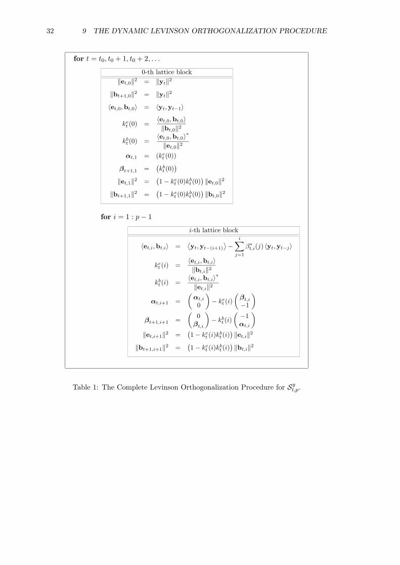
32 9 THE DYNAMIC LEVINSON ORTHOGONALIZATION PROCEDURE
for t = t0, t0 + 1, t0 + 2, . . .
0-th lattice block‖et,0‖2 = ‖yt‖2
‖bt+1,0‖2 = ‖yt‖2
〈et,0,bt,0〉 = 〈yt,yt−1〉
ket (0) =
〈et,0,bt,0〉‖bt,0‖2
kbt (0) =
〈et,0,bt,0〉∗
‖et,0‖2
αt,1 = (ket (0))
βt+1,1 =(kb
t (0))
‖et,1‖2 =(1− ke
t (0)kbt (0)
)‖et,0‖2
‖bt+1,1‖2 =(1− ke
t (0)kbt (0)
)‖bt,0‖2
for i = 1 : p− 1
i-th lattice block
〈et,i,bt,i〉 =⟨yt,yt−(i+1)
⟩−
i∑j=1
β∗t,i(j) 〈yt,yt−j〉
ket (i) =
〈et,i,bt,i〉‖bt,i‖2
kbt (i) =
〈et,i,bt,i〉∗
‖et,i‖2
αt,i+1 =(αt,i
0
)− ke
t (i)(βt,i
−1
)βt+1,i+1 =
(0βt,i
)− kb
t (i)(−1αt,i
)‖et,i+1‖2 =
(1− ke
t (i)kbt (i))‖et,i‖2
‖bt+1,i+1‖2 =(1− ke
t (i)kbt (i))‖bt,i‖2
Table 1: The Complete Levinson Orthogonalization Procedure for Syt,p.

9.4 The Complete Levinson Orthogonalization Procedure 33
‖bt0,0‖2 = ‖yt0−1‖2
for t = t0 : t0 + p− 2 (Order buildup)
0-th lattice block
for i = 1 : t− t0
i-th lattice block
for t = t0 + p− 1, t0 + p, . . . (Full order p)
0-th lattice block
for i = 1 : p− 1
i-th lattice block
Table 2: The Complete Levinson Orthogonalization Procedure for Syt,p with Order
Buildup.
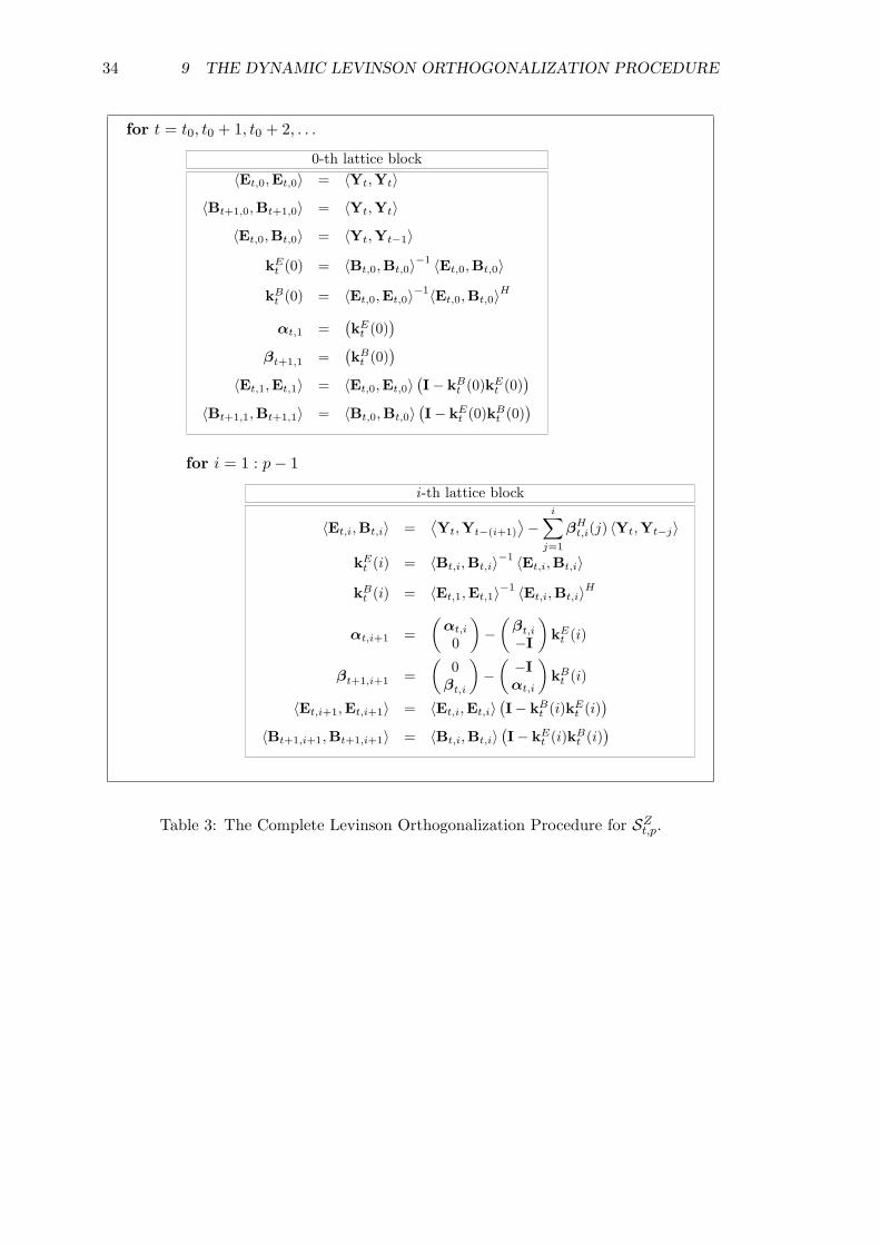
34 9 THE DYNAMIC LEVINSON ORTHOGONALIZATION PROCEDURE
for t = t0, t0 + 1, t0 + 2, . . .
0-th lattice block〈Et,0,Et,0〉 = 〈Yt,Yt〉
〈Bt+1,0,Bt+1,0〉 = 〈Yt,Yt〉
〈Et,0,Bt,0〉 = 〈Yt,Yt−1〉
kEt (0) = 〈Bt,0,Bt,0〉−1 〈Et,0,Bt,0〉
kBt (0) = 〈Et,0,Et,0〉−1〈Et,0,Bt,0〉H
αt,1 =(kE
t (0))
βt+1,1 =(kB
t (0))
〈Et,1,Et,1〉 = 〈Et,0,Et,0〉(I− kB
t (0)kEt (0)
)〈Bt+1,1,Bt+1,1〉 = 〈Bt,0,Bt,0〉
(I− kE
t (0)kBt (0)
)for i = 1 : p− 1
i-th lattice block
〈Et,i,Bt,i〉 =⟨Yt,Yt−(i+1)
⟩−
i∑j=1
βHt,i(j) 〈Yt,Yt−j〉
kEt (i) = 〈Bt,i,Bt,i〉−1 〈Et,i,Bt,i〉
kBt (i) = 〈Et,1,Et,1〉−1 〈Et,i,Bt,i〉H
αt,i+1 =(αt,i
0
)−(βt,i
−I
)kE
t (i)
βt+1,i+1 =(
0βt,i
)−(−Iαt,i
)kB
t (i)
〈Et,i+1,Et,i+1〉 = 〈Et,i,Et,i〉(I− kB
t (i)kEt (i)
)〈Bt+1,i+1,Bt+1,i+1〉 = 〈Bt,i,Bt,i〉
(I− kE
t (i)kBt (i)
)
Table 3: The Complete Levinson Orthogonalization Procedure for SZt,p.

9.4 The Complete Levinson Orthogonalization Procedure 35
〈Bt0,0,Bt0,0〉 = 〈Yt0−1,Yt0−1〉
for t = t0 : t0 + p− 2 (Order buildup)
0-th lattice block
for i = 1 : t− t0
i-th lattice block
for t = t0 + p− 1, t0 + p, . . . (Full order p)
0-th lattice block
for i = 1 : p− 1
i-th lattice block
Table 4: The Complete Levinson Orthogonalization Procedure for SZt,p with Order
Buildup.

36 REFERENCES
References
[1] Erwin Kreyszig: Introductory functional analysis with applications, John Wiley &Sons, 1998.
[2] Lasloo Mate: Hilbert space methods in science and engineering, Adam Hilger, 1989.
[3] Peter Brockwell and Richard A. Davis: Time series: Theory and methods, Springer–Verlag, 1987.
[4] G. W. Stewert: Introduction to Matrix Computations, Academic Press, 1973.
[5] G. H. Golub and C. F. Van Loan: Matrix Computations, John Hopkins UniversityPress, 1989.
[6] N. Levinson, The Wiener RMS Error Criterion in Filter Design and Prediction, J.Math. Physics, vol. 25, pp. 261–278, 1947.
[7] E. Karlsson and M. H. Hayes, Least Squares Modeling of Linear Time–VaryingSystems: Lattice Filter Structures and Fast RLS Algorithms, IEEE Trans Acoustic,Speech and Signal Processing, vol. ASSP-35, No. 7, pp. 994–1014, July 1987.
[8] S. Haykin: Adaptive Filter Theory, Third Ed., Prentice Hall, 1996.