The Geometry of Hurwitz SpaceThe Harvard community has made this

article openly available. Please share howthis access benefits you. Your story matters

Citation Patel, Anand Pankaj. 2013. The Geometry of Hurwitz Space. Doctoraldissertation, Harvard University.

Citable link http://nrs.harvard.edu/urn-3:HUL.InstRepos:11124835

Terms of Use This article was downloaded from Harvard University’s DASHrepository, and is made available under the terms and conditionsapplicable to Other Posted Material, as set forth at http://nrs.harvard.edu/urn-3:HUL.InstRepos:dash.current.terms-of-use#LAA

The Geometry of Hurwitz Space

A dissertation presented

by

Anand Pankaj Patel

to

The Department of Mathematics

in partial fulfillment of the requirementsfor the degree of

Doctor of Philosophyin the subject of

Mathematics

Harvard UniversityCambridge, Massachusetts

April 2013

© 2013 – Anand P. PatelAll rights reserved.

I dedicate this thesisto my grandparents and Devin

Dissertation Advisor: Joseph Harris Anand Pankaj Patel

The Geometry of Hurwitz Space

Abstract

We explore the geometry of certain special subvarieties of spaces of branched covers which

we call the Maroni and Casnati-Ekedahl loci. Our goal is to understand the divisor theory

on compactifications of Hurwitz space, with the aim of providing upper bounds for slopes of

sweeping families of d-gonal curves.

iii

Contents

Acknowledgements vi

1. Introduction 1

1.1. Objects of study 4

1.2. The Maroni and Casnati-Ekedahl loci 6

1.3. The associated Hirzebruch surfaces 8

1.4. The decomposition of H3,g by Maroni loci 13

1.5. The decomposition of H4,g by Maroni loci 15

1.6. The Casnati-Ekedahl loci C(F) ⊂ H4,g 21

1.7. Irreducibility of some Maroni loci 24

1.8. Degree 5 covers 27

1.9. Further Directions 32

2. Expressing Hurwitz Space as a Quotient 33

2.1. The Picard Rank Conjecture 33

2.2. From Severi varieties to Hurwitz spaces 37

2.3. A comparison of two conjectures 41

3. Compactifying Hurwitz Space 45

3.1. The admissible cover compactification Hd,g 46

3.2. Boundary Divisors in Hd,g 47

3.3. The decorated dual graph 48

3.4. Some more examples 49

3.5. Admissible Reduction 52

3.6. Independence of the boundary divisors 54

3.7. Partial pencils 54

4. Enumerative Geometry 61

4.1. The natural divisor classes on Hd,g 61

4.2. Slope bounds 66

iv

4.3. Slope bounds: d = 3 70

4.4. Slope bounds: d = 4 78

4.5. Slope bounds: d = 5 85

4.6. Some numerical observations 93

4.7. The congruence conditions on (g, d) 94

4.8. A final fun example 95

References 95

v

Acknowledgements

I first acknowledge the tremendous influence that my advisor, Joe Harris, has had on my

mathematical and personal life. He showed me many examples during graduate school, but

his best examples were: 1) his limitless devotion to his students, 2) his endless patience and

enthusiasm, and 3) his unwavering support.

Secondly, I must acknowledge the fact that I learned most of what I know from conver-

sations with Anand Deopurkar, my “academic elder brother.” Many of the results of this

thesis come from conversations I’ve had with him during graduate school. For this, I am

very grateful.

Thirdly, I must acknowledge the support provided to me by Dawei Chen and Maksym

Fedorchuk during my transition into the post-doctoral world.

Of course I must acknowledge the Ultra-Pro group of characters of the fourth floor whose

warm friendship kept me sane throughout graduate school: Oleg, Jerry, Anand, Toby

(spelling?), George, Cheng-Chiang, Erick, Gabriel, Eric, Matthew Woolf, the other Matthew

Woolf, Simon (fifth floor, but it’s ok), Pei-Yu, Yunqing, Francesco, Alex, etc...

Finally, I acknowledge the infinite love with which my parents brought me up and sup-

ported me.

vi

1. Introduction

The moduli space of genus g curves, Mg, has been a central object of study in algebraic

geometry for over a century. Classically, geometers studied a curve C by considering, roughly

speaking, all of the embeddings of C to projective spaces. For example, it was well known

that all projective curves C can be realized as a plane curve of some degree having only nodes

as singularities, and such planar representations were used to demonstrate the unirationality

of Mg for g ≤ 10.

There was another way to realize an algebraic curve - not as sitting inside a projective

space, but as a simply-branched covering of the projective line α : C −→ P1. Fixing the

degree d, genus g, and branch locus determines finitely many covers α : C −→ P1 with the

given invariants, so the dimension of the space of such coverings, Hurwitz space Hd,g, is three

less than the number of branch points, or 2g + 2d− 5. By studying the monodromy of the

branch point map Br : Hd,g −→M0,b, Clebsch proved the irreducibility of Hd,g, and thereby

gave the first proof of the irreducibility of Mg, since every genus g curve admits a map to

P1 of some uniform large degree.

In the late 70’s Harris and Mumford published one of the most celebrated results about

Mg - that it is of general type for g ≥ 22 [14]. The technique of proof boiled down to

computing the classes of particular effective divisors in the rational Picard group of the

Deligne-Mumford compactificationMg. These divisors were intimately related to the spaces

of admissible covers, Hd,g, a compactification of Hd,g. Specifically, for odd genera g = 2k+1,

Harris and Mumford considered the divisor Dk+1 consisting of the closure of the locus of

curves possessing a degree k + 1 map to P1, i.e. the image of the natural forgetful map

F : Hk+1,g −→ Mg. For even genera g = 2k, the Gieseker-Petri divisor GP1k+1, which

can be realized as the branch locus of the (generically finite) map F : Hk+1,g −→ Mg,

played an analogous role. Our ultimate goal is to understand the effective divisor theory of

compactifications of Hurwitz space. The ramification divisor of the forgetful map F will be

one of the two “types” of effective divisors we will study. In fact, one of the results we will

1

see in this first chapter is that this ramification divisor is always irreducible, hence the same

is true for the Gieseker-Petri divisors.

The divisor theory of Hd,g turns out to be more interesting (and less understood) when

d is small compared to g, and our general investigation naturally occurs in this range. The

starting point of our exploration is a classical construction, which we now describe.

By the “geometric” interpretation of Riemann-Roch, for any [α : C −→ P1] ∈ Hd,g the

fibers of α span Pd−2’s in Pg−1, the canonical space of C. The totality of these Pd−2’s forms

the associated scroll containing C.

In this way we obtain a function:

Ψ:

Degree d Covers−→

Isomorphism types of Pd−2-bundles over P1

By fixing an isomorphism type of associated scrolls, (which we will eventually denote by

PE), we consider the closed Maroni locus M(E) ⊂ Hd,g, consisting of the (closure of the)

locus of covers [α : C −→ P1] whose associated scroll is isomorphic to PE . The Gieseker-

Petri divisors GP1k+1 mentioned earlier will be instances of these subvarieties M(E) ⊂ Hd,g.

One central question which we explore in the first chapter is: What, in general, can be said

about the geometry of the subvarieties M(E)?

It will become quite apparent that the study of the Maroni loci will naturally lead to the

study of certain other subvarieties which we call the Casnati-Ekedahl loci. In fact, as we will

point out in the last section, the study of these two sets of subvarieties is only the first step

in understanding a fascinating and completely mysterious decomposition of Hurwitz space

by higher syzygy loci.

We will begin our explorations in chapter 1 by recalling a structure theorem, due to Casnati

and Ekedahl [3], which describes the resolution of the ideal of the curve C in its associated

scroll. This will immediately lead to the central objects of study: the Maroni loci M(E)

and the Casnati-Ekedahl loci C(F). We then examine the necessary conditions (mainly due

to Ohbuchi), Conditions 1, 2, and 3, for a scroll PE to occur as an associated scroll of some

2

cover, i.e. in the image of Ψ. (Condition 3 is actually first mentioned in section 3, where we

study the degree 4 case carefully, thereby giving some motivation for the condition.)

We have devoted a few sections of chapter 1 to the study of Maroni and Casnati-Ekedahl

loci in low degree cases. We provide examples showing that the Maroni loci are often not

of expected codimension, and may have multiple components. We also classify all reducible

Casnati-Ekedahl loci in H4,g, and describe the components of these loci in terms of the

resolvent cubic morphism.

In section 1.7, we provide the most general result known about the geometry of the Maroni

loci in Hd,g. The key input comes from a theorem of Tyomkin [23] stating that all Severi

varieties on all Hirzebruch surfaces are irreducible. Using this theorem, we prove that the

only Maroni divisor are the “expected” ones, i.e. although some Maroni loci may have larger

dimension than expected, there is never an instance of an unexpected Maroni divisor. As a

corollary to the main theorem in section 5, we deduce the irreducibility of the Gieseker-Petri

divisors GP1k+1.

Section 1.8 explores what is known about the Maroni and Casnati-Ekedahl loci in H5,g. In

particular, we will see that all Casnati-Ekedahl loci are irreducible, and that there are “no

unexpected Casnati-Ekedahl divisors”. This result, along with the aforementioned theorem

on the nonexistence of unexpected Maroni divisors is used in proving the first results of

chapter 2, which we now summarize.

In chapter 2 we introduce the well-known “Picard Rank Conjecture” for Hd,g stating that

the rational Picard group is trivial. When the degree d is large compared to the genus g,

Mochizuki [18] shows that the conjecture is equivalent to Harer’s theorem [13]. We verify

the Picard Rank Conjecture for H3,g, H4,g, and H5,g. Section 2.2 relates a conjecture about

Picard groups of Severi varieties on Hirzebruch surfaces with the Picard Rank Conjecture.

As a corollary, we recover some results of Edidin [12].

Chapter 3 is devoted to the study of the boundary divisors occurring in the admissible

cover compactification Hd,g. We prove that the boundary divisors are independent, thereby

putting the divisor calculations of chapter 4 on firm ground. We also introduce the idea of a3

partial pencil family - a technique of constructing test families which have “controlled” and

easily determined intersections with boundary divisors. Partial pencil families are heavily

used in chapter 4.

Chapter 4 investigates enumerative questions about the geometry of Hurwitz space. In

particular, we find the classes of the Maroni and Casnati-Ekedahl divisors, and use them

to produce sharp upper bounds for slopes of sweeping 4-gonal and 5-gonal curves. These

results generalize the result of Stankova [22].

We work over an algebraically closed field k of characteristic 0.

1.1. Objects of study. The Hurwitz space (or “small” Hurwitz space) Hd,g is the Deligne-

Mumford stack of dimension 2d + 2g − 5 which represents the functor of degree d, genus g

simply-branched covers of P1. More precisely, for a scheme S, the objects of Hd,g(S) are

diagrams:

Cα//

ϕ

P

π

S

where π is a P1-bundle, ϕ is a flat family of smooth genus g curves, and α is a finite, flat,

degree d map which restricts to a simply-branched map on all geometric fibers of ϕ.

By associating to a cover [α : C −→ P1] ∈ Hd,g its branch divisor [B ⊂ P1] ∈ M0,b, we

arrive at the branch morphism

Br : Hd,g −→M0,b

which is finite and unramified. For us, M0,b will denote the moduli space of unordered

b-tuples of distinct points in P1, modulo PGL2 equivalence.

In this first chapter, we will be dealing primarily with the geometry of the underlying

coarse space. The distinction between the stack and coarse space will not be relevant until

chapter 4, where we will compute intersection numbers. Since the coarse space of M0,b is

affine, the (coarse) Hurwitz space is also an affine variety of dimension 2d+ 2g − 5.4

Now let [α : C −→ P1] be any cover and consider the sequence of sheaves on P1:

0 −→ OP1 −→ α∗OC −→ E∨ −→ 0

Dualizing, and using Serre duality to identify (α∗OC)∨ ' α∗ωα, we obtain:

0 −→ E −→ α∗ωα −→ OP1 −→ 0

Pulling back to C and composing with the relative evaluation map evα : α∗α∗ωα −→ ωα, we

obtain the map of sheaves on C:

evα|E : α∗E −→ ωα

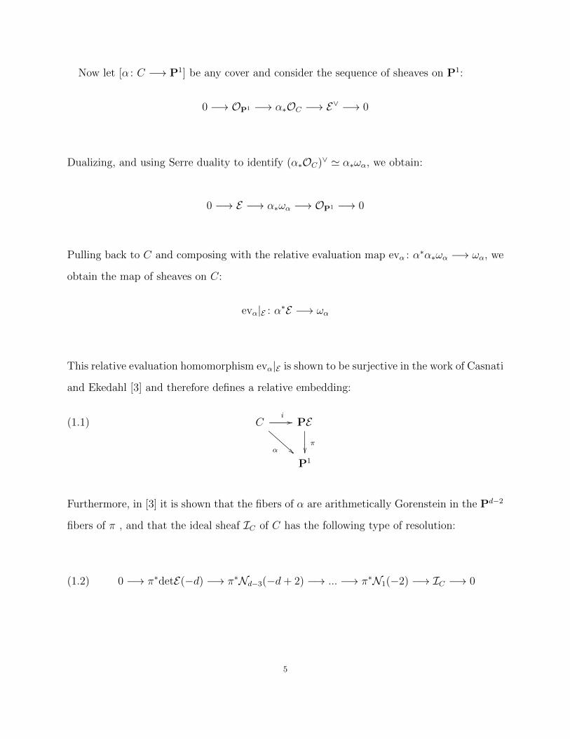
This relative evaluation homomorphism evα|E is shown to be surjective in the work of Casnati

and Ekedahl [3] and therefore defines a relative embedding:

(1.1) Ci//

α

PE

π

P1

Furthermore, in [3] it is shown that the fibers of α are arithmetically Gorenstein in the Pd−2

fibers of π , and that the ideal sheaf IC of C has the following type of resolution:

(1.2) 0 −→ π∗detE(−d) −→ π∗Nd−3(−d+ 2) −→ ... −→ π∗N1(−2) −→ IC −→ 0

5

In every fiber of π, this resolution restricts to the minimal resolution of d general points in

Pd−2. There is a natural duality among the syzygy bundles: Ni ' (Nd−2−i)∨ ⊗ det E .

We will call E the reduced direct image of α, and

F := N1 = π∗ IC(2)

the bundle of quadrics of α. To emphasize the dependence on α, we will sometimes use the

notation Eα and Fα. We have the following exact sequence relating the two bundles:

0 −→ F −→ S2E −→ α∗ω⊗2α −→ 0

Throughout this thesis, the natural hyperplane class associated to a projective bundle

will be denoted by ζ, and a fiber class will be denoted by f . We use post-Grothendieck

conventions for projective bundles: Surjections E −→ L −→ 0 onto line bundles correspond

to geometric sections s : P1 −→ PE .

1.2. The Maroni and Casnati-Ekedahl loci. For a fixed rank d − 1, degree g + d − 1

locally free sheaf E on P1 , we define the subvariety M(E) as:

M(E) :=

[α : C −→ P1] ∈ Hd,g | Eα = E

Maroni [17] first implicitly considered these subvarieties in the trigonal setting, so we will

call M(E) the Maroni locus of E .

Similarly, for a fixed F of the appropriate rank and degree define C(F) as:

C(F) :=

[α : C −→ P1] ∈ Hd,g | Fα = F

6

We will call this subvariety the Casnati-Ekedahl locus of F . The main objective of this

first chapter is to understand general geometric properties ofM(E) and C(F). In particular,

we will review three conditions for the non-emptiness of M(E) essentially due to [20]. (Our

method of arriving at these conditions is more geometric.) We will also see several examples

which illustrate the complexity of the geometry of these varieties.

1.2.1. Preliminary Observations. We will now guide the reader through some basic properties

of the bundles associated to a cover. Much of what follows is simply a unified treatment of

well-known observations and results. We will provide references as we go - anything stated

without reference is new (at least as far as the author can tell).

From the basic setup it follows that E is a rank d− 1 locally free sheaf of degree g+ d− 1

and that the rank of F is d(d−3)2

. Furthermore, from the exact sequence:

0 −→ F −→ S2E −→ α∗ω⊗2α −→ 0

we see that the degree of F is (d− 3)(g + d− 1).

As a locally free sheaf on P1, we may write

E = OP1(a1)⊕OP1(a2)⊕ ...⊕OP1(ad−1)

where a1 ≤ a2 ≤ ... ≤ ad−1. The integers ai (or slight variants thereof) are known as

“scrollar invariants” in the existing literature. (The reader should note that knowing the

sequence (a1, ...ad−1) is equivalent to knowing the sequence of numbers h0(C, α∗O(m)).) We

first notice that, if C is connected, all ai’s will be positive.

We immediately provide a first example which will be useful for us in the future.

Example 1.1 (Rational Covers). Let α : R −→ P1 be a degree d cover where R is a rational

curve. The degree of Eα is d − 1. Therefore, since all summands of Eα are positive, we7

conclude that

Eα = O(1)⊕d−1

The bundle PE is isomorphic to the split bundle Pd−2×P1. Projection onto Pd−2 embeds

R as a rational normal curve of degree d − 2. In particular, the curve R ⊂ PE rests as a

(d, 1) curve in the surface S = P1 × P1 embedded in Pd−2 × P1 via the relative Veronese

embedding (relative to the first projection) of degree d− 2. This allows us to compute Fα.

By considering the sequence

0 −→ IS(2) −→ IR(2) −→ IR⊂S(2) −→ 0

it easy to show that

Fα = O(1)⊕d−3 ⊕O(2)⊕(d−22 )

We simply note that the global sections of Fα(−2) correspond to quadrics in Pd−2 containing

the rational normal curve R.

The line bundle OPE(1) ⊗ π∗OP1(−ad−1) is then the lowest degree effective hyperplane

divisor class on PE . Since C is arithmetically Gorenstein over P1, the fibers of α are always

in general linear position in Pd−2. In particular, OPE(1)⊗ π∗OP1(−ad−1) must restrict to a

line bundle of nonnegative degree on C. Observing that OPE(1)|C = ωα, we obtain the first

condition on the (d− 1)-tuple (a1, a2, ..., ad−1):

Condition 1. If E is the reduced direct image of a cover [α : C −→ P1] with C irreducible,

then

ad−1 ≤2g + 2d− 2

d

Now we shift our attention to the minimal degree of a summand, a1. In order to see the

condition on a1, we will need a construction which is interesting in its own right and which

will be appear again in another chapter.

1.3. The associated Hirzebruch surfaces. The construction which we describe in this

section can first be found in the work of Ohbuchi. We would like to give two interpretations8

of the construction, one which is “algebraic”, and one which is “geometric.” The geometric

interpretation seems to be new. Consider the inclusion of sheaves

OP1 ⊕OP1(−a1) → α∗OC .

From this we obtain a map of OP1-algebras,

Spec (OP1 ⊕OP1(−a1)⊕OP1(−2a1)⊕OP1(−3a1)⊕ ...) −→ Spec (α∗OC)

thereby defining a morphism j : C −→ Fa1 whose image avoids the directrix σ.

1.3.1. Geometric realization. We view C as naturally embedded C ⊂ PE . Pick a surjection

E −→ O(a1) −→ 0

This corresponds to picking a section σ ⊂ PE of minimal degree (with respect to any fixed

hyperplane divisor).

The section σ together with the curve C provide d+1 points σt∪αt in the fibers Pd−2t ⊂ PE ,

where t is representing a coordinate on P1. Since we assume that the map α : C −→ P1

is simply branched, monodromy considerations show that the general such set of d + 1

points must be in general linear position. Therefore, there is a unique rational normal curve

Rt ⊂ Pd−2t passing through the d+ 1 points σt ∪ αt for t ∈ P1 general.

The closure of the union of these rational normal curves Rt is a birationally ruled surface

S ⊂ PE containing C and σ. When we blow down those components of the fibers of

π : S −→ P1 which avoid the section σ, we arrive at a Hirzebruch surface Fn, and a birational

map j : C −→ Fn. In fact, it is not hard to show that n = a1, and that this geometric

procedure provides the same morphism j : C −→ P1 which was constructed algebraically in

the previous subsection.

Either way, if we assume that j is birational onto its image then we obtain a condition

on the integer a1. The image j(C) has fixed divisor class d · τ where τ is the unique section9

class satisfying τ 2 = a1. Comparing the geometric genus of j(C) with its arithmetic genus,

we immediately arrive at:

Condition 2. If E is the reduced direct image of a cover [α : C −→ P1], and if α does not

factor as the composite of two finite maps, then

a1 ≥g + d− 1(

d2

) .

(Note that for prime d or for a simply branched cover, one can obviously drop the extra

hypothesis about α.)

We will arrive at the final nontrivial condition on E , due to Ohbuchi, after we explore

degree 4 Hurwitz spaces in section 1.5. For now we observe that, since Hd,g is irreducible,

the general cover [α : C −→ P1] ∈ Hd,g has a well-defined generic reduced direct image Egen

and bundle of quadrics Fgen. One may expect that these bundles are as balanced as possible.

As we will see in Proposition 1.1, this will always be true for the generic reduced direct image

Egen, but unfortunately will not always hold for bundles of quadrics, as the following example

shows:

Example 1.2 (h1(EndFgen) 6= 0). Consider the Hurwitz space Hd,4 with d ≥ 6, and let

[α : C −→ P1] ∈ Hd,4 be a general cover. The reduced direct image is

E = O(1)⊕d−5 ⊕O(2)⊕4

The bundle of quadrics F is a subbundle of

S2E = O(2)⊕M ⊕O(3)⊕N ⊕O(4)⊕10

of rank d(d−3)2

and degree (d− 3)(d+ 3).

In the factorization

Ci//

α

PE

π

P1

10

The linear system |ζ − 2f | on PE restricts to the complete canonical series on C. Fur-

thermore, the system |2ζ − 4f | is simply the symmetric square of the system |ζ − 2f |, and

so we see that there is exactly one nonzero section of OPE(2ζ − 4f) vanishing on C. There-

fore, O(4) occurs as a summand of F exactly once, and it is a maximal degree summand.

The remaining summands of F cannot all be O(3)’s, since the degrees would not add up.

Therefore, h1(EndFgen) 6= 0.

The reader may notice that the reason we took g = 4 is simply because the canonical

model of a genus 4 curve is contained in a quadric, thereby forcing F to have O(4) as a

summand. From here, we simply took d large enough so that F was forced to also have O(2)

summands.

The example above indicates that there are hidden surprises in the analysis of C(F) for d

large compared to g. On the other hand, for g large compared to d, which will be the central

concern of most of this thesis, we are more fortunate:

Theorem 1.3 (Generic Behavior). Egen is rigid, i.e. h1(End Egen) = 0. Fgen is rigid for

H4,g and H5,g. For g sufficiently large compared to d, Fgen is rigid.

Proof. The proof will be via degeneration. We will use our understanding of rational covers

to deduce the first part of the proposition.

Write g = (k− 1)(d− 1) + e, where 0 ≤ e < (d− 1), and consider a chain of k+ 1 rational

curves P := ∪k+1i=1 P1

i . Above P we will construct an appropriate degree d, arithmetic genus g

cover, component by component. For each i ≤ k, choose a general simply branched, degree

d rational cover αi : Ri −→ P1i , and glue the Ri appropriately (always generically) so as to

construct a finite, arithmetic genus (k − 1)(d− 1) cover αL : R −→ ∪ki=1P1. (The subscript

L should be read as “left.” )

Above the final component P1k+1, consider a disjoint union of d−e−1 “constant” rational

curves ∪jAj along with a rational curve B mapping [e+1: 1] onto P1k+1. Let X := tjAj tB

be the disjoint union, and denote by αR : X −→ P1k+1 the degree d map which is the union

of degree 1 maps on the components Aj and the degree e + 1 map on B. We now choose a11

generic gluing Y = X ∪ R, maintaining a finite map α : Y −→ P which restricts to αL and

αR.

As we have already seen, the reduced direct image EαL restricts on every component P1i ,

(i ≤ k), as

Eαi = O(1)⊕d−1

Furthermore, the reduced direct image of αR is

EαR = O(1)⊕e ⊕O⊕d−e−1

It follows that the reduced direct image Eα satisfies h1(P, End Eα) = 0. By upper semi-

continuity, we deduce the same for Egen.

Now we switch to the proof of the statements regarding Fgen. Let us consider the broken

curve R of arithmetic genus (k − 1)(d − 1) which was used above. R is built from rational

covers Ri, and as we have seen, these covers have bundles of quadrics Fαi of the form:

Fαi = O(1)⊕d−3 ⊕O(2)⊕(d−22 )

Recall that EαL is the reduced direct image of the broken cover β : R −→ ∪ki=1P1i .

We now “transfer” all information into one fiber of the broken scroll PE . Consider the

d points Z := R1 ∩ R2 lying above the node P11 ∩ P1

2, and let Pd−2Z denote the fiber of PE

containing Z. The rational curves R1 and R2 both project into Pd−2Z to a pair of rational

normal curves passing through Z. By repeatedly projecting, we may view all of the Ri

as rational normal curves in the projective space Pd−2Z . The resulting curve is abstractly

isomorphic to R itself, with each component a general rational normal curve of degree d− 2.

For each component Ri, consider the vector space Vi ⊂ H0(Pd−2Z ,O(2)) of quadrics containing

Ri. Let Zi,i+1 := Ri ∩Ri+1, let VZi,i+1be the space of quadrics containing Zi,i+1. Clearly, Vi

and Vi+1 are subspaces of VZi,i+1.

12

It is easy to see that the calculation of h1(EndF) depends on the relative positions of the

vector spaces Vi in the direct sum ⊕iVZi,i+1. For general choices of Ri, we can guarantee that

all intersections will be proper, and therefore h1(EndF) will be zero for the resulting curve.

Now suppose γ : E −→ P1 is an elliptic degree d cover. The bundle of quadrics for γ is

easily seen to be perfectly balanced:

Fγ = O(2)⊕d(d−3)

2

Therefore, by gluing together chains of elliptic covers to chains of rational covers, we may

deduce that h1(EndFgen) = 0 for all genera of the form g = ad + b(d − 1) with a, b ≥ 0.

Eventually, we may express every sufficiently large integer g as such a combination.

We can prove h1(EndFgen) = 0 for H4,g and H5,g by similar arguments. As we’ve seen,

elliptic covers always have perfectly balanced bundles of quadrics. Therefore, for H5,g, for

example, we must only show that Fgen is rigid for 0 ≤ g ≤ 4. We may then obtain the

result for all genera by constructing chains of genus 1 covers followed by a genus 0, 1, 2, 3,

or 4 cover. The low genus cases are easily established using similar reasoning as in Example

1.2 above, so we leave them out.

Very little is known about M(E) or C(F) in general. However, for low degrees (3, 4, and

perhaps 5), a fairly complete picture can be obtained. Furthermore, by studying the low

degree cases carefully, we will begin to see interesting phenomenon occurring in the geometry

of these varieties. For this reason, we devote a few sections to the study of these low degree

cases before returning to arbitrary d.

1.4. The decomposition of H3,g by Maroni loci. We briefly review the geometry of the

decomposition of H3,g by the Maroni loci. In this case, Conditions 1 and 2 are equivalent in

light of the constraint a1 + a2 = g + 2. The difference a2 − a1 is known in the literature as

the Maroni invariant of the cover α.13

Suppose [α : C −→ P1] ∈ H3,g has reduced direct image E . The associated scroll PE is a

Hirzebruch surface, so C as a member of the fixed linear series |3ζ− (g+2)f | on PE . (Recall

that ζ will always denote the divisor class associated to OPE(1), and f will denote the class

of a fiber.) The normal bundle NC/PE is nonspecial, i.e. H1(C,NC/PE) = 0, therefore basic

deformation theory tells us that every deformation of PE carries C along with it. If we

introduce the map on (mini)versal deformation spaces

Ψ: Def(α) −→ Def(PE)

we conclude that Ψ is formally smooth, and in particular if PE ′ specializes to PE , then

M(E) ⊂M(E ′). Therefore, a dense open subset of M(E) can be presented as the quotient

of an open subset U ⊂ |3ζ − (g + 2)f | by G = AutPE , the automorphism group of the

surface PE . This greatly simplifies the study of the Maroni loci, and allows for a rather

complete understanding of their geometry. We have

Proposition 1.4. If E = O(a1)⊕O(a2) is such that a1 <g+2

3, then M(E) is empty. Other-

wise, the Maroni loci M(E) ⊂ H3,g are irreducible and of expected codimension h1(End E).

If E specializes to E ′, then M(E ′) ⊂ M(E), and, away from the locus of covers having

automorphisms, the union of such M(E ′) forms the singular locus of M(E).

Proof. The linear series |3ζ−(g+2)f | contains smooth divisors if and only if a1 ≥ g+23

, hence

the first statement. The rest follows from the formal smoothness of Ψ, and the well-known

description of the decomposition of the deformation space Def(PE) by isomorphism type of

scroll.

Therefore, we see that the decomposition (in fact, stratification) of H3,g by Maroni loci

behaves exactly as we would expect and hope. As we will see in the next section, almost

every aspect of Proposition 1.4 fails in higher degree.

14

1.4.1. The Maroni Divisor. When the genus g = 2k is even, the general reduced direct

image Egen is perfectly balanced with Egen = OP1(k + 1) ⊕ OP1(k + 1). Therefore, for the

special bundle Ediv := OP1(k)⊕OP1(k+ 2) the Maroni locus M :=M(Ediv) is irreducible of

codimension 1 and is appropriately called the Maroni divisor in the existing literature.

When k = 2, the Maroni divisor M ⊂ H3,4 is the locus of Petri curves, i.e. those genus 4

curves which lie on a quadric cone Q ⊂ P3 in canonical space. The resolution of the quadric

cone is the scroll PEdiv.

The Maroni divisor plays a central role in understanding the birational geometry of the

locus of trigonal curves T3 ⊂Mg [10] [22]. In particular, by computing the class of its closure

in T 3 ⊂Mg, Stankova [22] produced the sharp upper bound of 7 + 6g

for the slope δ/λ of a

sweeping curve in T 3. We will generalize Stankova’s result in chapter 4 after studying the

divisor theory on the Hurwitz space of admissible covers, Hd,g for larger d.

1.5. The decomposition of H4,g by Maroni loci. The decomposition of H4,g by Maroni

loci is more complicated. We begin by reviewing the essential (for our purposes) geometric

property of a degree four cover [α : C −→ P1] ∈ H4,g: The domain curve C is a complete

intersection in the P2-bundle PE .

1.5.1. The geometry of a degree 4 cover. For [α : C −→ P1] ∈ H4,g, the natural factorization

(1.2) from section 1

Ci//

α

PE

π

P1

expresses C ⊂ P(E) as a family of 4 points varying in the fibers of the P2-bundle PE .

Furthermore, the Casnati-Ekedahl resolution (1.2) from Section 1.1 has the following form:

(1.3) 0 −→ π∗detE(−4) −→ π∗F(−2) −→ IC −→ 015

where F is the rank 2 bundle of quadrics (conics) associated to α. Since F splits, C is

always a complete intersection of two relative conic divisors in the bundle PE . Specifically,

if F = OP1(u)⊕OP1(v), where u+ v = g + 3, then C is a complete intersection of a pair of

divisors Qu ∈ |2ζ − uf | and Qv ∈ |2ζ − vf |. We will assume that u ≤ v.

In order to understand the geometry of M(E), we first consider the subvarieties

M(E ,F) :=

[α : C −→ P1] ∈ H4,g | Eα = E ,Fα = F

In other words, we consider the closure of the locus of covers with a prescribed reduced direct

image E and quadric bundle F . The loci M(E ,F) are easily described, given the fact that

degree four covers occur as complete intersections of relative quadrics:

Proposition 1.5. M(E ,F) is an irreducible subvariety of H4,g of codimension h1(End E) +

h1(EndF)− h1(F∨ ⊗ S2E).

Proof. A general section, modulo scaling, of the bundle F∨ ⊗ S2E provides a complete in-

tersection Qu ∪ Qv in the scroll PE . Applying automorphisms in AutPF/P1 gives rise to

the same complete intersection. Secondly, we must mod out by automorphisms of the scroll

PE . Straightforward calculation yields the result.

SinceM(E) =⋃iM(E ,Fi) for finitely many Fi, we can establish the dimension/irreducibility

of M(E) if we know the inclusion relationships among the subvarieties M(E ,Fi).

With this in mind, let us fix E = OP1(a1) ⊕ OP1(a2) ⊕ OP1(a3) with a1 ≤ a2 ≤ a3, and

a1 + a2 + a3 = g + 3. Condition 1 says that a3 ≤ g+32

, which is equivalent to saying that

the second gap m2 := a3 − a2 must be less than or equal to the lowest degree, a1. What is

slightly less obvious is that the first gap m1 := a2 − a1 also cannot exceed a1, which we now

explain.16

Suppose, on the contrary, that m1 > a1, or equivalently 2a1 < a2. Then, since a3 ≤ g+32

,

we must have a1 + a3 < 2a2. Now consider S2E :

S2E = OP1(2a1)⊕OP1(a1 + a2)⊕OP1(a1 + a3)

⊕OP1(2a2)⊕OP1(a2 + a3)⊕OP1(2a3)

The degrees of the summands as presented are now in increasing order. Let X, Y, Z denote

the relative homogeneous “coordinates” of PE corresponding to the projections of E to the

summands OP1(a1),OP1(a2), and OP1(a3), respectively. If F = OP1(u)⊕OP1(v), (u ≤ v) is

a potential quadric bundle for α, then u ≤ 2a1 must hold, otherwise the section [X : Y : Z] =

[1 : 0 : 0] would be contained in the intersection of Qu and Qv. Therefore, v ≥ g + 3− 2a1.

However, this forces the equation of Qv to be an expression of the form

Qv = pY 2 + qY Z + rZ2

where the degrees of (p, q, r) are (2a2 − v, a2 + a3 − v, 2a3 − v). In other words, Qv, viewed

as fibered over P1 under the projection π, will be a family of reducible conics.

Let γ : Qνv −→ P1 be the natural map from the normalization Qν

v of Qv to P1, and let

γ : Qνv −→ E −→ P1 be its Stein factorization. The curve C = Qu ∩ Qv is then a double

cover of E. This means that C will necessarily be bi-hyperelliptic, i.e. the cover α : C −→ P1

will factor though E, which forces the branching to be non-simple. This provides a simply

geometric reason explaining some of the results in [8].

Remark 1.6. In fact, we can easily describe the genus of the curve E: The number of “double

lines” occurring in the family of reducible conics [π : Qv −→ P1] is the number of zeros of

the polynomial q2−4pr, which is 2(a2 +a3)−2v. Since the cover C is assumed to be smooth,

we must have u = 2a1, so this implies that the number of double lines is 2a1. Therefore, the

genus of E is a1 − 1.17

The conlusion is: for simply branched degree 4 covers, m1 ≤ a1. In fact, Ohbuchi shows

more generally for all degrees d and genera g:

Condition 3 (Ohbuchi [20]). For every [α : C −→ P1] ∈ Hd,g, the ith difference mi := ai+1−ai

never exceeds a1.

(We emphasize: The only way Condition 3 can fail to be satisfied is if α is composite, but

we are only considering simply branched covers.)

Now we will present some examples to illustrate the complexity of the decomposition by

Maroni loci.

Example 1.7 (Failure of Expected Codimension). : Suppose a1 <g+2

5, and consider the

bundle E = OP1(a1) ⊕OP1(2a1) ⊕OP1(g + 3 − 3a1). An argument parallel to that used to

arrive at Condition 3 shows that the only possible bundle of quadrics F has degrees u = 2a1

and v = g + 3− 2a1. However, Proposition 1.5 and direct calculation gives

codim E = codimM(E ,F)

= h1(End E)− (g + 2− 5a1)

< h1(End E)

It then remains to show that there are actually smooth curves arising as Qu ∩ Qv, but this

is an application of Bertini’s theorem on Qv.

Example 1.8 (Failure of Irreducibility). Consider E = OP1(3) ⊕ OP1(5) ⊕ OP1(7). Then

both F0 = OP1(6)⊕OP1(9) and F1 = OP1(5)⊕OP1(10) are bundles of quadrics for covers

in M(E) ⊂ H4,12. Calculating the codimensions of M(E ,Fi) using Proposition 1.5 gives

codimM(E ,Fi) = h1(End E)18

Therefore, M(E) has expected dimension, yet is reducible with components M(E ,Fi). In

fact, M(E ,F1) ∩M(E ,F2) = ∅, because a cover [α : C −→ P1] ∈ M(E ,F0) ∩M(E ,F1)

must have a reduced direct image E ′ 6= E which is a specialization of E . Therefore, a1 = 3

must drop to 2, but this violates Condition 2. This is the first example of a reducible Maroni

locus. It is also the first example of a disconnected Maroni locus.

Example 1.9 (Failure of Expected Codimension and Irreducibility). Consider E = OP1(4)⊕

OP1(7) ⊕ OP1(10). The two possible bundles of quadrics are F0 = OP1(8) ⊕ OP1(13) and

F1 = OP1(7) ⊕ OP1(14). M(E ,Fi) both have codimension 1 less than expected, and form

the two irreducible components ofM(E). The two components do not intersect in H4,18 just

as in the previous example.

We can trivially generalize these examples to show that M(E) can have more than two

components: Fix integers j < m and let E = OP1(m + j) ⊕ OP1(2m + j) ⊕ OP1(3m + j).

The possible bundles of quadrics are Fi = OP1(2m + 2j − i) ⊕OP1(4m + j + i), 0 ≤ i ≤ j.

Each component M(E ,Fi) has codimension h1(End E) +m− j − 1.

These examples indicate that both reducibility and unexpected dimension are to be ex-

pected when considering the subvarieties M(E). However, all is not lost - we can at least

establish irreducibility for a particular collection of M(E). We will do this in the next

section. For now, we provide a classical example:

Example 1.10 (The g = 6 Gieseker-Petri locus). A general genus 6 curve C rests in its

canonical embedding as a quadric hypersurface section of a unique quintic Del Pezzo surface

S ⊂ P5. The (closure of the) locus of curves C lying on a singular Del Pezzo surface forms

the Gieseker-Petri divisor GP14 ⊂M6.

If we realize S as Blp1,p2,p3,p4P2, the blow up of the plane at 4 general points, then the

divisor class of C is [C] = 6H −∑

i 2Ei. Therefore, C is realized as a sextic plane curve19

having 4 nodes. The five different g14’s on C are given by the linear series |H − Ei| and

|2H −∑

iEi|. If p1 becomes incident with p2, or if three (say p2, p3, p4) of the four points

become collinear, then the Del Pezzo surface S becomes singular, acquiring an ordinary

double point. Furthermore, the five distinct g14’s no longer remain distinct: In the first case,

|H − E1| coincides with |H − E2|, while in the second case |2H −∑

iEi| = |H − E1|.

On the other hand, in H4,6 the general reduced direct image is Egen = OP1(3)⊕OP1(3)⊕

OP1(3). The Maroni divisor is M(Ediv), where Ediv := OP1(2)⊕OP1(3)⊕OP1(4).

Fix a cover [α : C −→ P1] ∈ H4,6 and consider the sequence of sheaves on C:

0 −→ TC −→ α∗TP1 −→ Nα −→ 0

The boundary map

δ : H0(C,Nα) −→ H1(C, TC)

is the differential of the map on versal deformation spaces

F : Def(α) −→ Def(C)

If Eα = Egen, the kernel ker δ is 3 dimensional (coming from infinitesimal automorphisms of

P1. However, when Eα = Ediv, ker δ becomes 4 dimensional, so F is ramified. Therefore, the

Maroni divisor is the ramification divisor of the forgetful map F : H4,6 −→M6. Notice that

this analysis does not depend on the pair g, d satisfying g = 2(d− 1), so the Maroni divisor

is always the ramification divisor of the dominant map F : Hd,2(d−1) −→M2(d−1).

Returning to our specific setting, consider [α : C −→ P1] ∈ H4,6 such that Eα = Egen. The

only acceptable bundle of quadrics is F = OP1(4)⊕OP1(5). So, in PEα, C is the complete

intersection of Q4 ∈ |2ζ − 4f | and Q5 ∈ |2ζ − 5f |. Furthermore, the linear series |ζ − 2f |

restricts to ωC on C, and maps PEα to the geometric scroll mentioned in the Introduction.

Under |ζ − 2f |, Q5 embeds as the quintic Del Pezzo containing C.20

If Eα = Ediv, then the linear series |ζ − 2f | contracts the section [X : Y : Z] = [1 : 0 : 0]

which is contained in Q5 as a −2 curve, and therefore we recover the singular Del Pezzo

surface which contains C. For our purposes, the important take away from this classical

example is that the Maroni divisor dominates the Gieseker-Petri locus. We will revisit this

in general degree and genera later.

1.6. The Casnati-Ekedahl loci C(F) ⊂ H4,g. The Casnati-Ekedahl loci first appear in

H4,g. In the natural factorization

Ci//

α

PE

π

P1

we may interpret the bundle map β : PF −→ P1 as the family of conics containing the fibers

of α (four points) in each fiber of π. There is a distinguished curveD ⊂ PF parametrizing the

singular conics containing the fibers of α. The restriction β : D −→ P1 clearly has degree 3,

and is simply branched precisely above the points where α is branched. By Riemann-Hurwitz,

the genus of D is g + 1. In fact the function field, K(D), is isomorphic to the “resolvent

cubic” field(s) associated to the extension of function fields K(P1) ⊂ K(C). Furthermore,

since degF = g + 3 = (g + 1) + 2 = g(D) + 2, F must be the reduced direct image Eβ of

[β : D −→ P1] ∈ H3,g+1. In this way, we obtain the classical morphism

Φ: H4,g −→ H3,g+1

Φ([α : C −→ P1]) := [β : D −→ P1]

which we will call the resolvent cubic map. The Recillas construction [21] naturally identifies

the fiber Φ−1([β : D −→ P1]) with the nontrivial 2-torsion points in the Jacobian Jac(D).

Therefore Φ is etale, of degree 22(g+1) − 1.21

So we immediately see that Casnati-Ekedahl loci have a beautifully simple geometric

description in terms of the resolvent cubic morphism:

Φ: H4,g −→ H3,g+1

C(F) = Φ−1(M(F))

Therefore, it follows from Proposition 1.4 that the Casnati-Ekedahl loci are always of the

expected codimension h1(EndF). Furthermore if F specializes to F ′, then C(F ′) ⊂ C(F).

The question of irreducibility is only slightly more subtle. Recall the irreducible varieties

M(E ,F) :=

[α : C −→ P1] ∈ H4,g | Eα = E ,Fα = F

The varieties M(E ,F) serve as building blocks for Maroni and Casnati-Ekedahl loci, in the

sense that if a Maroni or Casnti-Ekedahl locus is irreducible, the components must obviously

be of the form M(E ,F). Since all Casnati-Ekedahl loci are pure dimensional, we can count

dimensions, finding instances when the codimension ofM(E ,F) is equal to h1(EndF). From

Proposition 1.5 we see that

h1(End E) = h1(F∨ ⊗ S2E)

must hold. By checking all cases, we may find all instances of reducible Casnati-Ekedahl

loci.

Proposition 1.11. C(F) is irreducible if and only if g ≡ 0 mod 3 and

F = O(g + 3

3

)⊕O

(2(g + 3)

3

)(In other words, C(F) is the smallest dimensional nonempty Casnati-Ekedahl locus.)

In these situations, C(F) has precisely two components:

C(F) =M(Egen,F) ∪M(Ediv,F)

(In other words, the Maroni divisor M(Ediv) does not intersect C(F) properly.22

Proof. We simply check all instances of pairs of bundles (E ,F) which satisfy the equality

h1(End E) = h1(F∨ ⊗ S2E)

We leave this to the reader, as it is not very enlightening.

We recover the observation made by Vakil in [24]: The preimage of the Maroni divisor

under the resolvent cubic map Φ: H4,3 −→ H3,4 has exactly two components.

Proposition 1.11 sheds light on the monodromy of the resolvent cubic map Φ. By the

Recillas construction, we may view the resolvent cubic morphism Φ: H4,g −→ H3,g+1 as

the total space of the local system of (Z/2Z)-valued relative first homology of the universal

curve over H3,g+1. Using this description, we can think about the reducibility of C(F) as a

statement about the monodromy of Lefschetz pencils.

We look at the following situation: On the Hirzebruch surface Fk consider the linear

system |3τ + af |, a ≥ 0. Here τ is the unique section class which avoids the directrix σ. Let

U ⊂ |3τ + af | be the open subset parametrizing smooth divisors, i.e. the complement of the

discriminant divisor. Let u : C → U be the universal curve over U , and fix a point x ∈ U .

Proposition 4.1 then says that the action of π1(U) on R1u∗(Z/2Z)x \0 is transitive, unless

a = 0, in which case there are exactly two orbits.

Let P ⊂ |3τ+af | be a general pencil containing x, and denote by PU the intersection P∩U .

It is a well-known fact, due to Lefschetz [16], that the natural map g : π1(PU) −→ π1(U)

is surjective. Therefore, we may replace u : C → U with the total space of the pencil

p : X → P . X = BlBFk is the blow up of Fk along the base locus B of the pencil P . Let Cx

be the fiber of p at x.

Assume, for the moment, that all singular fibers of the pencil p are simply nodal. Under

this assumption, by copying Lefschetz’s argument for the monodromy of plane curves, one

can similarly show that π1(PU) acts on H1(Cx,Z) as the full symplectic group Sp2g(Z). The

general pencil in the linear series |3τ + af | will have simply nodal singular elements if and23

only if a 6= 0. When a = 0, the linear series |3τ | is trivial when restricted to the directrix σ,

so any pencil of 3τ curves will violently split off the directrix σ at a certain point. This is

where the obstruction for full monodromy comes from.

Another explanation for why there are exactly two orbits in R1u∗(Z/2Z)x \ 0 comes

from applying adjunction to a 3τ curve C. We see that

ωC = OFk(C +KFk)|C = 2(k − 1)f |C

so the line bundle (k − 1)fC is a theta characteristic for C which is even or odd depending

on the parity of k. Therefore, we may translate all theta characteristics to the two-torsion

of the Jacobian J(C), and furthermore, we can do this globally over the parameter space U .

The monodromy action must preserve even and odd theta characteristics, and Proposition

1.5 tells us that the action on these two subsets of R1u∗(Z/2Z)x \ 0 is transitive.

1.7. Irreducibility of some Maroni loci. The associated Hirzebruch surface construction

j : C −→ Fa1 from Section 1.3 allows us to establish the irreducibility of a particular class of

Maroni loci. Before going on, let us make a definition: We will call a nondecreasing sequence

(a1, a2, ..., ad−1) of d− 1 positive integers acceptable if it satisfies Conditions 1, 2, 3 and the

degree constraint a1 + a2 + ...+ ad−1 = g + d− 1.

What we have seen from our explorations and from the work of Ohbuchi is that all re-

duced direct image bundles for simply branched covers must have an acceptable sequence of

summands. However, it seems to be an open question whether the converse holds: Are all

acceptable sequences realized by a reduced direct image for a simply branched cover? The

only result known to us seems to be a theorem of Coppens [6] which we now explain.

Fix k := a1, an integer satisfying Condition 2. Let (k, a′2, a′3, ..., a

′d−1) be the unique

acceptable sequence maximizing the weighted sum (d − 1)k + (d − 2)a2 + (d − 3)a3 + (d −

4)a4 + ...+ ad−1. The reader should think of this acceptable sequence as the most “general”

among acceptable sequences having k as the first coordinate. This can be made precise by24

an upper semi-continuity for the corresponding bundles. Define

Egen(k) := O(k)⊕O(a′2)⊕O(a′3)⊕ ...⊕O(a′d−1)

The main theorem of Coppens [6], reformulated into our language, is:

Theorem 1.12 (Coppens [6]). The Maroni locus M(Egen(k)) ⊂ Hd,g is nonempty.

The bundles Egen(k) are particularly nice, because it turns out that any reduced direct

image E ′ having O(k) as a minimal degree summand will be a specialization of Egen(k), i.e.

M(E ′) ⊂M(Egen(k)). This will be a consequence of the stronger statement thatM(Egen(k))

is irreducible.

Theorem 1.13 (Irreducibility of M(Egen(k))). For k <⌊g+d−1d−1

⌋, M(Egen(k)) ⊂ Hd,g is

an irreducible subvariety of codimension g − (d − 1)k + 1. Furthermore, any reduced direct

image E ′ having OP1(k) as a least degree summand will be a specialization of Egen(k), and

furthermore, M(E ′) ⊂M(Egen(k)).

Proof. The proof of the theorem relies on Coppens theorem mentioned above, and the fol-

lowing result of Tyomkin [23]:

Theorem 1.14 (Tyomkin [23]). All Severi varieties parametrizing irreducible curves on

Hirzebruch surfaces are irreducible and of expected dimension.

Let [α : C −→ P1] ∈ Hd,g be any cover such that k is a minimal degree of a summand of

Eα. (The summand may not be unique.) A choice of inclusion O(−k) ⊂ E∨α gives rise to a

map j : C −→ Fk which is birational onto its image, by the “associated Hirzebruch surface

construction” in section 1.3. Letting V denote the Severi variety parametrizing irreducible,

geometric genus g curves in the linear system |dτ | on Fk, we arrive at a rational map

q : V −→ Hd,g

25

whose image contains the cover α. Tyomkin’s theorem says that V is irreducible, and hence

so is the image q(V ) ⊂ Hd,g.

Coppens’ theorem cited above then shows that the generic point of q(V ) parametrizes

covers α such that Eα = Egen(k). Therefore, q(V ) =M(Egen(k)).

Finally, assuming k <⌊g+d−1d−1

⌋, the choice of inclusion O(−k) ⊂ E∨α will be unique, so the

map q : V −→ Hd,g is birationally a G-torsor over its image, where G = AutFk/P1. By

Tyomkin’s theorem, we know that V is of expected dimension. A direct calculation then

gives the statement about the codimension of M(Egen(k)).

Two important observations follow from Theorem 1.13. First, we have:

Theorem 1.15 (No unexpected Maroni divisors). The only divisorial Maroni locus isM(Ediv(k)),

where

Ediv(k) := O(k)⊕O(k + 1)⊕d−3 ⊕O(k + 2)

Proof. By Theorem 1.13 above, the codimension of the Maroni locusM(Egen(k)) is g− (d−

1)k + 1 when k <⌊g+d−1d−1

⌋. By setting this equal to 1, we see that

g = (d− 1)k

which means that Egen(k) is precisely Ediv(k) from the statement of the theorem.

It remains to check that there is no reduced direct image E ′ which: (1) is not of the form

Egen(k), (2) has minimal summand k =⌊g+d−1d−1

⌋, and (3) is such that M(E ′) is divisorial.

The first two conditions on E ′ imply that

E ′ = O(k)r ⊕N

for some r ≥ 2.

Recall the map

q : V −→ Hd,g

26

from the proof of Proposition 5.1. Above the locus M(E ′), the map q (rationally) factors

through a Pr−1-bundle PGr −→M(E ′) parametrizing “choices of inclusions”O(−k) ⊂ (E ′)∨.

Since we assume r ≥ 2, the dimensions of the fibers of q are jumping, so Tyomkin’s

irreducibility theorem for the Severi variety V implies thatM(E ′) must not be a divisor.

We will call M(Ediv(k)) the Maroni divisor. In the special case k = 2, we observe:

Corollary 1.16 (Irreducibility of the Gieseker-Petri divisors GP1d). Assume g = 2(d −

1). The Maroni divisor M(Ediv(2)) is irreducible and dominates the Gieseker-Petri divisor

GP1d ⊂Mg under the forgetful map F : Hd,g −→Mg. Therefore, GP1

d is irreducible.

Proof. The corollary follows from the observations made in Example 1.10, and Theorem

1.13.

1.7.1. An interesting open question. As we see from the irreducibility theorem above, the

subvarieties M(Egen(k)) are, in general, not of expected codimension, yet we may still ask

the following question:

Question: Is it always true that M(Egen(k − 1)) ⊂M(Egen(k))?

1.8. Degree 5 covers. We now explore the Maroni and Casnati-Ekedahl loci in H5,g. The

main tool is a well-known linear algebraic description of degree 5 covers, which we review.

Let [α : C −→ P1] ∈ Hd,g be any cover. The Casnati-Ekedahl resolution from section 1.1

has the form:

0 −→ det E(−5) −→ π∗F∨ ⊗ det E(−3) −→ π∗F(−2) −→ IC −→ 0

The central map between rank 5 bundles is well-known to be skew symmetric, i.e., after

pushing down to P1 under π defines a nonzero section s of the bundle ∧2F ⊗ E ⊗ det E∨.

The curve C is the “rank 2” locus of this skew symmetric matrix.27

The matrix associated to the section s may be written as

M =

0 L1,2 L1,3 L1,4 L1,5

−L1,2 0 L2,3 L2,4 L2,5

−L1,3 −L2,3 0 L3,4 L3,5

−L1,4 −L2,4 −L3,4 0 L4,5

−L1,5 −L2,5 −L3,5 −L4,5 0

where the sections Li,j restrict to linear forms on the P3-fibers of the scroll π : PE −→ P1.

The equations cutting out C are the five 4× 4 sub-Pfaffians of the matrix M .

Geometrically, we may view the construction of degree 5 covers as follows. The section s

may be viewed as a surjection

s : ∧2 F∨ −→ E ⊗ det E∨ −→ 0

which provides an inclusion of bundles:

P(E ⊗ det E∨) ' PE → P(∧2F∨)

In the P9-bundle P(∧2F∨), we may consider the locus of rank 2 tensors, also known as

the relative Grassmanian:

G := Grass(2,F∨) → P(∧2F∨)

The original curve C is simply the intersection C = PE ∩G ⊂ P(∧2F∨).

As in section 1.6, we define the subvarieties

M(E ,F) :=

[α : C −→ P1] ∈ H5,g | Eα = E ,Fα = F

Casnati [4] proves a general Bertini-type existence theorem for degree 5 covers. We state

the version we need as:

28

Theorem 1.17 (Casnati [4]). If the bundle ∧2F ⊗ E ⊗ det E∨ is globally generated, then

there exists a cover [α : C −→ P1] ∈ H5,g such that Eα = E and Fα = F .

The coarse geometric properties of the subvarieties M(E ,F) are now easily established.

Proposition 1.18. The subvarietiesM(E ,F) are irreducible and of codimension h1(End E)+

h1(EndF)− h1(∧2F ⊗ E ⊗ det E∨).

Proof. The proof is completely analogous to the proof of Proposition 1.5. We begin with the

projective space of “skew symmetric matrices” P(∧2F ⊗E ⊗ det E∨), and then quotient out

successively by AutPF/P1 and AutPE to obtain a birational description ofM(E ,F). The

proposition follows easily from here.

In section Proposition 1.11, we encountered some reducible Casnati-Ekedahl loci in H4,g.

However, it is a remarkable fact that Casnati-Ekedahl loci are always irreducible in H5,g:

Proposition 1.19. All Casnati-Ekedahl loci C(F) ⊂ H5,g are irreducible.

Proof. In the P9-bundle P(∧2F∨), we consider all P3-subbundles Λ ' PE having the ap-

propriate class in the Chow ring A∗P(∧2F∨). The totality of these subbundles forms an

irreducible open subset of the appropriate Hilbert scheme. The conditions that force Λ ∩G

to be a smooth, nondegenerate genus g curve are all open conditions, so the proposition

follows.

As a consequence of the two propositions above, we have:

Theorem 1.20 (No unexpected Casnati-Ekedahl divisors). The only divisorial Casnati-

Ekedahl loci are of the form C(Fdiv), where Fdiv = O(m)⊕O(m+ 1)⊕3 ⊕O(m+ 2).

Proof. A divisorial Casnati-Ekedahl locus C(F) must be of the form M(E ,F) for some E ,

by Proposition 1.19. By the Theorem 1.15 on “No unexpected Maroni divisors”, we know

that E must either be Egen or Ediv. We may eliminate the latter case by Casnati’s existence29

theorem cited above: There will always exist covers [α : C −→ P1] such that Eα = Ediv, and

Fα = Fgen. However, M(Ediv,Fgen) is clearly not C(F) for any F .

So we may assume E = Egen. We will indicate how the task of “checking all relevant cases”

can be reduced to a much simpler check.

First, we observe that F must be imbalanced, i.e. h1(EndF) 6= 0. Write

F = O(x1)⊕ ...⊕O(x5)

with x1 ≤ x2 ≤ ... ≤ x5 and suppose

Egen = O(k)⊕r ⊕O(k + 1)4−r

Let us interpret a section of the bundle ∧2F ⊗ E ⊗ det E∨ as a skew symmetric matrix

M =

0 L1,2 L1,3 L1,4 L1,5

−L1,2 0 L2,3 L2,4 L2,5

−L1,3 −L2,3 0 L3,4 L3,5

−L1,4 −L2,4 −L3,4 0 L4,5

−L1,5 −L2,5 −L3,5 −L4,5 0

where Li,j ∈ H0(P1, E ⊗det E∨⊗O(xi+xj)). In other words, the Li,j restrict to linear forms

on the fibers of π : PE −→ P1 with “coefficients” read off by the splitting type of the rank

4 bundle E ⊗ det E∨ ⊗O(xi + xj).

In PE , the curve C is cut out by the 4× 4 sub-Pfaffians of the matrix M . Suppose both

L1,2 and L1,3 are zero. Then the Pfaffian of the sub matrix obtained by eliminating the fifth

row and column is

Q5 = L1,2L3,4 − L1,3L2,4 + L2,3L1,4 = L2,3L1,4

which is a reducible quadric. This would force the cover α : C −→ P1 to have smaller

monodromy group.

30

Therefore, the maximum of the (two) degrees of the summands of E⊗(det E∨)⊗O(x1 +x3)

must be nonzero, meaning

x1 + x3 ≥ (g + 4)− (k + 1)

The xi + xj are increasing, so we deduce the same inequality for almost all pairs:

(1.4) ∀ i, j 6= 1, 2, xi + xj ≥ (g + 4)− (k + 1)

Since E is balanced, this means that h1(E ⊗ (det E∨)⊗O(x1 +x3)) = 0. Therefore, all of the

contribution of h1(∧2F ⊗ E ⊗ det E∨) comes from the smallest 4 summands, i.e.

h1(∧2F ⊗ E ⊗ det E∨) = h1(E ⊗ det E∨ ⊗O(x1 + x2))

Now, the divisorial assumption, along with Proposition 6.2 say that

1 = h1(End E) + h1(EndF)− h1(∧2F ⊗ E ⊗ det E∨)

Under our assumptions, h1(End E) = 0, so we simply must show

h1(EndF)− h1(∧2F ⊗ E ⊗ det E∨) = 1

However, from the considerations above, we know that this is equivalent to

h1(EndF)− h1(E ⊗ det E∨ ⊗O(x1 + x2)) = 1

From here, it is straightforward to check using (1.4) that in the remaining few possibilities

if h1(EndF) ≥ 2 then

h1(EndF)− h1(E ⊗ det E∨ ⊗O(x1 + x2)) ≥ 2

31

Remark 1.21. In the next chapter we will prove the Picard Rank Conjecture for degrees 3, 4,

and 5, i.e. that PicQH3,g = PicQH4,g = PicQH5,g = 0. The theorem above will be needed

for the degree 5 case.

1.9. Further Directions. The reader may notice that the Casnati-Ekedahl resolution (1.2)

from section 1.1 actually provides a much more comprehensive association

Φ:

degree d covers−→

⌊d2

⌋−tuples of vector bundles on P1

whose formula is:

Φ([α : C −→ P1]) := (Eα,Fα,N2,N3, ...)

We may define higher syzygy loci to be the fibers of this association and its projections to

the various factors. The resulting decomposition of Hurwitz space seems, in full generality,

to be intractable, but we still think it a worthy subject of research.

As we will see in the final chapter, as far as “divisorial” enumerative questions are con-

cerned, the bundles E and F play a more fundamental role than the rest of the syzygy

bundles. Before we tackle enumerative questions however, we will need to work in a com-

pactification of Hurwitz space. Understanding the admissible cover compactification will be

the subject of the third chapter.

32

2. Expressing Hurwitz Space as a Quotient

The goals of this chapter are to (1) establish the Picard Rank Conjecture of the Hurwitz

space parametrizing simply branched covers of P1 of degree 3, 4, and 5, and (2) understand

the relationship between the Picard Rank Conjecture and the Diaz-Harris conjectures about

Picard groups of Severi varieties.

As far as the first goal is concerned, the strategy is the same in all three cases: We will

begin with a vector space V which parametrizes “presentations of ideals of covers in their

scrolls”. Then we will quotient out successively by “equivalence of presentations”, and then

by automorphisms of the associated scroll PE . Many of the ideas of the proof come from

conversations with Anand Deopurkar.

The second goal is achieved by analyzing the “associated Hirzebruch surface” construction

from chapter 1, section 1.3. Via the associated Hirzebruch surface construction, we may think

of Hurwitz space as a “quotient” of an appropriate Severi variety, and this explains the title

of the chapter.

The proofs of the statements in this chapter will require a few results from chapters 3 and

4. The results referred to are not dependent on the results of this chapter, as the reader can

check for themselves.

2.1. The Picard Rank Conjecture. The main outstanding conjecture about Picard groups

of Hurwitz spaces is:

Conjecture 2.1 (Picard Rank Conjecture). The rational Picard group PicQHd,g is zero for

all pairs (d, g).

The proofs of the statements in this chapter will require a few results from chapter 4. The

results referred to in chapter 4 are not dependent on the results of this chapter, as the reader

can check for themselves.

For pairs (d, g) satisfying d ≥ g+1, Mochizuki [18] showed that the Picard Rank Conjecture

is equivalent by Harer’s theorem stating that PicQMg = Q〈λ〉 [13]. However, for d small33

compared to g, the conjecture is mostly wide open. In this section, we prove the conjecture

for d = 3, 4, and 5.

2.1.1. The Picard Rank Conjecture for H3,g. For completeness, and to illustrate the ideas

which will be used in the other two cases, we will review the proof of the Picard Rank

Conjecture in degree 3. We let Hd,g denote the space of all degree d covers [α : C −→ P1]

having smooth domain C. It is a quasi projective variety containing the simple Hurwitz space

Hd,g as a dense open subset. The complement Hd,g\Hd,g is the union of two divisors T,D

which generically parametrize covers having a triple ramification point and covers having

“double”, or (2,2) ramification above a single point in P1, respectively. Of course, when

d = 3 the divisor D does not exist.

As we have seen, the generic reduced direct image sheaf E = Egen is rigid, i.e. h1(End E) =

0. The vector space

V = H0(OPE(3ζ − (g + 2)f)) = H0(P1,S3E(−g − 2))

parametrizes “equations for trigonal curves” C embedded in the Hirzebruch surface PE via

the natural Casnati-Ekedahl factorization.

The complement of the locus of smooth curves in the linear system PV is an irreducible

divisor (the discriminant divisor), and therefore PicQ U = 0. We have the natural map

q : U −→ H3,g

which is (away from a codimension 2 subset) a G-torsor, where G = AutPE . The image

q(U) ⊂ H3,g is the locus of covers [α : C −→ P1] satisfying Eα = Egen.

We then appeal to a theorem which is due to Knopf, Kraft, and Vust [15]:

Theorem 2.2 (Knop, Kraft, Vust [15]). Let q : X −→ Y be a Zariski-locally trivial G-torsor,

G a connected algebraic group. Let PicGX denote the the space of G-linearized line bundles

on X. Then the pullback map q∗ : Y −→ PicGX is injective. Furthermore, there exists an34

exact sequence:

(2.1) χ(G) −→ PicGX −→ PicX

where χ(G) is the character group of G.

As a consequence of the theorem, we notice that the following inequality holds:

(2.2) rk PicQ Y ≤ rk PicQX + rkχ(G)

Applying Theorem 1 in our context, we conclude

rk PicQ q(U) ≤ rkχ(G)

We divide our analysis into two cases: g even, and g odd.

When g is even, the bundle PEgen is perfectly balanced. Therefore, G = PGL2 × PGL2,

which means χ(G) = 0. The complement of the image M = H3,g\q(U) is an old friend, the

Maroni divisor M :=M(Ediv). Proposition 1 and Proposition 2 from chapter 4 tell us that

the divisor classes of M and T are multiples of each other in PicQHd,g. This allows us to

conclude that PicQH3,g = 0 for g even, because the complement H3,g \ H3,g is precisely the

divisor T .

When g is odd, we have χ(G) = Z, while the complement H3,g\q(U) is codimension 2 by

Proposition 2.1 in chapter 1. Therefore,

rk PicQH3,g = rk PicQ q(U) ≤ 1

However, Proposition 1 from chapter 4 tells us that the divisor class of T is nontrivial, so

rk PicQH3,g = 1, and the Picard Rank Conjecture follows.

2.1.2. The Picard Rank Conjecture for H4,g. We follow exactly the same line of reasoning as

above. We let E = Egen, and F = Fgen and consider

V = H0(P1,F∨ ⊗ S2E)35

The vector space V , modulo scaling parametrizes “ideals of complete intersections” in

the scroll PE of the type we saw in section 3 of chapter 1. As before, there is a dense

open subset U ⊂ PV parametrizing smooth complete intersections whose complement is a

divisor. Therefore, PicQ U = 0. We may change parametrizations of the same ideal, which

means we must quotient out by G1 = AutPF/P1. Then we must further quotient out by

G2 = AutPE to obtain the total composite quotient map:

q : U −→ H4,g

There are two possibilities for χ(G1) depending on the parity of g (splitting type of F) and

two possibilities for χ(G2) depending on whether g is a multiple of three or not. We will

explain how we deal with one of the four possible scenarios, leaving the other three to the

reader.

If g is odd, then Fgen is perfectly balanced, and G1 ' PGL2, which has no nontrivial

characters. If, furthermore, g is divisible by 3, then Egen will be perfectly balanced, and so

G2 will be PGL2 × PGL3, which also has no nontrivial characters. The Maroni divisor M

and the Casnati-Ekedahl divisor CE will comprise two components of the complement of

the image q(U). Theorem 1 tells us

rk PicQ q(U) ≤ rk PicQ U + rkχ(G1) + rkχ(G2) = 0

However, Proposition 2 in chapter 4 and the theorem on independence of boundary divisors

in chapter 3 together tell us that: 1) M and CE are linear combinations of T and D in

PicQH4,g and 2) the divisors T and D are linearly independent in PicQH4,g.

To summarize: Theorem 1 provides an upper bound for the Picard rank. This upper bound

is then realized by exhibiting enough independent divisor classes in the image. The divisorial

components of the complement of the image q(U) are either the Maroni or Casnati-Ekedahl

divisor, which are shown to be linear combinations of T and D in chapter 4.

36

2.1.3. The Picard Rank Conjecture for H5,g. We follow the same reasoning: Begin with

V = H0(P1,∧2F ⊗ E ⊗ detE∨)

the space of “skew symmetric matrices.” Consider the open set U ⊂ PV of matrices whose

rank 2 locus is a smooth curve. Again, PicQ U = 0. We quotient out by G1 = AutPF/P1,

and then by G2 = AutPE resulting in the map

q : U −→ H5,g

There are again 2 possibilities for χ(Gi) depending on whether or not the bundles Egen and

Fgen are perfectly balanced.

We conclude by the exact analogues of 1) and 2) from the previous section. One small point

to bring to the reader’s attention: In order to finish the argument, we must know whether

there exist unexpected divisorial Maroni or Casnati-Ekedahl loci. Thankfully, Theorem 1.15

and Theorem 1.20 guarantee that this does not happen.

2.2. From Severi varieties to Hurwitz spaces. In this section, we would like to un-

derstand a morphism relating Severi varieties on Hirzebruch surfaces with Hurwitz spaces.

Recall the construction of the “associated Hirzebruch surface” from chapter 1, section 1.3.

Let us write Egen = O(k)⊕r ⊕ O(k + 1)⊕d−r−1, and assume that r > 0. Then the map of

OP1-algebras given by

SpecSymO(−k) −→ Specα∗OC

provides a map

j : C −→ Fk

which factors the original covering α. Furthermore, the image of j avoids the directrix,

forcing the the divisor class [j(C)] to be dτ where τ is the section class satisfying τ 2 = k.

The space of all inclusions O(−k) ⊂ E∨, up to scalar multiplication, forms a projective space37

Pr−1. Therefore, once such an inclusion has been selected, the resulting map j : C −→ Fk is

determined up to the action of G = AutFk/P1.

Let V = V irrg,dτ be the Severi variety parametrizing irreducible, nodal curves of geometric

genus g in the linear series |dτ | and consider the natural map

q : V −→ Hd,g

which, to every nodal curve [X] ∈ V assigns the obvious d : 1 map from the normalization

Xν induced by the projection from Fk to P1. Notice that the image q(V ) is precisely the

locus of covers α : C −→ P1 such that the least degree of a summand of Eα is k. From the

theorem of “No unexpected Maroni divisors” Theorem 1.15, we observe that the complement

of the image q(V ) is a divisor if and only if r = d− 1.

2.2.1. A rephrasing of the Picard Rank Conjecture. Using the “quotient map” q, we will

relate the Picard groups of V and Hd,g. Although we have already introduced the Picard

Rank Conjecture, we will reformulate it in a more “intrinsic” way, following Diaz-Harris [11].

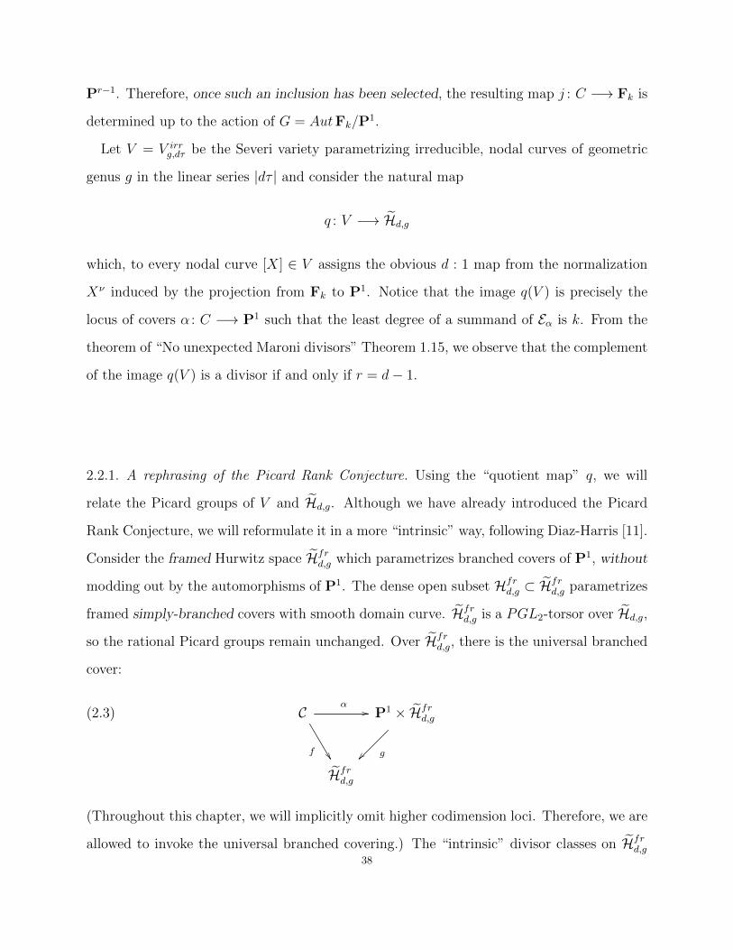
Consider the framed Hurwitz space Hfrd,g which parametrizes branched covers of P1, without

modding out by the automorphisms of P1. The dense open subset Hfrd,g ⊂ H

frd,g parametrizes

framed simply-branched covers with smooth domain curve. Hfrd,g is a PGL2-torsor over Hd,g,

so the rational Picard groups remain unchanged. Over Hfrd,g, there is the universal branched

cover:

(2.3) Cα

//

f

P1 × Hfrd,g

g

Hfrd,g

(Throughout this chapter, we will implicitly omit higher codimension loci. Therefore, we are

allowed to invoke the universal branched covering.) The “intrinsic” divisor classes on Hfrd,g

38

are those which are obtained “solely” from the diagram (2.3):

λH = c1(f∗c1(ωf ))

κH = f∗(c21(ωf ))

ξH := f∗(α∗c1(OP1(1)) · c1(ωf ))

(We include the subscript H to emphasize the context of working with Hurwitz space.)

Proposition 4.1 tells us that the Picard Rank Conjecture is equivalent to:

Conjecture H. The rational Picard group PicQ Hfrd,g is generated by the intrinsic classes

λH , κH , and ξH .

Next, we formulate the analogous conjecture for the Severi varieties V .

2.2.2. A conjecture for Severi varieties. The “small” Severi variety V parametrizing irre-

ducible, geometric genus g, nodal curves in the linear system |dτ | is not compact in codi-

mension one. Exactly as in Diaz-Harris [11], we must allow three types of codimension one

singular phenomenon to occur: cusps CU , tacnodes TAC, and triple points TP . We must

also allow curves to acquire an additional node, yielding the divisor which we will call ∆.

Unlike for Severi varieties on P2, we must also allow our curves to split off the directrix σ of

Fk, yielding the divisor of reducible curves, RED. Let

V := V ∪ CU ∪ TAC ∪ TP ∪∆ ∪RED

be the partial compactification of V . V is now compact in codimension one.

In order to formulate our conjecture, we would like to invoke the universal genus g curve

parametrized by V . However, we may not do so immediately, since there is no way, for

example, of distinguishing which subset of nodes of a curve parametrized by ∆ ought to be

normalized. As shown in Diaz-Harris [11], the solution to this problem is to work over the

normalization W of V . Then, we have a family of arithmetic genus g curves:39

(2.4) Cj//

ϕ

Fk × W

ψ

W

Let π : Fk −→ P1 denote the projection. The Picard group of Fk is generated by the class

of a fiber f , and the directrix σ. Following Diaz-Harris [11], we define the intrinsic divisor

classes to be:

λS = c1(f∗c1(ωϕ))

κS = f∗(c21(ωϕ))

ξS := f∗(j∗(f) · c1(ωϕ))

εS := f∗(j∗(σ) · c1(ωϕ))

ρS := f∗(j∗(σ · f))

Finally, we may formulate

Conjecture S. The rational Picard group PicQ W is generated by the intrinsic classes λS, κS, ξS, εS,

and ρS.

Letting W ⊂ W be the locus parametrizing irreducible curves, we immediately notice that

εS and ρS are both trivial in PicQW . The quotient morphism

q : W −→ Hfrd,g

will be the central tool used to prove the main result of the next section which will compare

Conjecture H and Conjecture S.40

2.3. A comparison of two conjectures. Now that we have this setup, we would like to

compare Conjecture H with Conjecture S using the quotient map q. We first show that

Conjecture H implies Conjecture S.

Lemma 2.3. Conjecture H implies Conjecture S for the appropriate Severi variety.

Proof. Conjecture H implies PicQHfrd,g = 0, by Proposition 4.1. Restrict attention to the

open subset U ⊂ Hfrd,g parametrizing covers [α : C −→ P1] satisfying Eα = Egen. If

Egen = O(k)⊕r ⊕O(k + 1)⊕d−r−1

then the complement of U has codimension two or more unless r = d− 1, in which case the

complement is the Maroni divisor M. In either case, PicQ U = 0, assuming Conjecture H.

Consider the quotient map

q : W −→ Hfrd,g

This map is not a G-torsor - it factors through the space which parametrizes “choices of

inclusions” O(−k) ⊂ E∨, or equivalently “choices of surjections” E −→ O(k) −→ 0. Re-

stricting our attention over the subset U ⊂ Hfrd,g, we can make this “choice of surjections”

space precise as follows.

Over the open set U×P1, the universal reduced direct image bundle Eα has a distinguished

surjection Eα −→ Gr −→ 0 onto the well-defined rank r bundle Gr which restricts toOP1(k)⊕r

on the fibers of g. The projective bundle PGr is the desired “choice of sections” space, and

by applying the “associated Hirzebruch surface” construction globally over PGr we arrive at

a family:

(2.5) Cj′

//

f ′

PGr × Fk

g′yyPGr

41

The quotient map q, when restricted to the preimage Y of U , factors as

q : Y −→ PGr −→ U

and the first map is a trivial G-torsor because the family (2.5) above provides a section.

Since PicQG = 0, we conclude that PicQ Y = Q〈ζ〉 if r > 1 and PicQ Y = 0 if r = 1.

Here ζ is the hyperplane class on PGr. In the space PGr, we may eliminate the choices of

surjections E −→ O(k) −→ 0 which lead to a triple point under the associated Hirzebruch

surface construction. This is a “horizontal” divisor in PGr, so eliminating it will reduce the

rational Picard group of Y to 0. Therefore, let Y ′ be Y \TP . Then, what we have concluded

is that PicQ Y′ = 0, assuming Conjecture H.

To recap: The open subset Y ′ ⊂ W is obtained by removing q-preimages of some divisors

in Hfrd,g along with the divisor TP . It is not hard to show (following Diaz-Harris [11]) that

the divisor TP is a combination of intrinsic divisor classes. Finally, observe that q∗(λH) =

λS, q∗(κH) = κS, and q∗(ξH) = ξS. This observation together with the conclusion that

PicQ Y′ = 0, implies Conjecture S.

Now we prove the opposite direction.

Lemma 2.4. Conjecture S for the appropriate Severi variety implies Conjecture H.

Proof. Let us first assume r < d − 1. We consider the open subsets Y ′ ⊂ Y ⊂ W , and

Uk ⊂ Hfrd,g defined as follows: Uk is the locus of covers α : C −→ P1 such that the least

degree of a summand of Eα is k. Y := q−1(Uk), where

q : W −→ Hfrd,g

is the quotient map, and Y ′ = Y \ TP .42

Let U ⊂ Uk be the locus of covers satisfying Eα = Egen = O(k)⊕r ⊕O(k + 1)⊕d−r−1. Put

Y ′′ := q−1(U). As before, we see that the quotient map q, when restricted to Y ′′, factors as

q : Y ′′ −→ PGr −→ U

The Pr−1-bundle PGr is the space of “choices of surjections” E −→ O(k) −→ 0, so the first

map is a G-torsor. Applying Theorem 2.2 to the first map gives

(2.6) rk PicQ PGr ≤ rk PicQ Y′′ + rkχ(G) = rk PicQ Y

′′ + 1

Now, if r > 1, then we observe that rk PicQ PGr = rk PicQ U + 1, so we obtain the

inequality

rk PicQ U ≤ rk PicQ Y′′

However, Conjecture S implies that PicQ Y′′ is generated by λS, κS, and ξS, which are all

pulled back from U via q. Therefore, we see that the inequality above must be an equality,

and Conjecture H follows.

The case r = d − 1 essentially requires the same argument. The only thing we need to

know in the end is that the Maroni divisor M is an intrinsic divisor in Hfrd,g. This follows

from Proposition 4.1. We let the reader spell it out. The interesting remaining case is r = 1,

which we now deal with.

Suppose r = 1, and consider the locally closed locus Z ⊂ Hfrd,g parametrizing covers

α : C −→ P1 satisfying

Eα = O(k)⊕2 ⊕O(k + 1)⊕d−4 ⊕O(k + 2)

An upper bound for the codimension of Z is h1(End Eα) = 2. Notice that the “space of

surjections” has jumped dimension to become a P1. Therefore, the preimage X := q−1(Z) ⊂

W is a divisor which is contracted under the quotient map. The divisor X must be nontrivial

in PicQW . X is visibly contained in the complement of Y ′′, and so, assuming Conjecture S,

43

we see that rk PicQ Y′ ≤ 2. From the inequality (6), we obtain

rk PicQ U ≤ rk PicQ Y′′ + 1 ≤ 3

(PGr is isomorphic to U .) Conjecture H follows by noting that λH , κH and ξH are indepen-

dent classes, which follows from results of chapter 3.

We have therefore proved the main theorem of the chapter:

Theorem 2.5 (A Comparison of Conjectures). The Picard Rank Conjecture for Hd,g is

equivalent to Conjecture H for Hfrd,g, which in turn is equivalent to Conjecture S for the

appropriate Severi variety.

Remark 2.6. By the work of Mochizuki [18], we know that Conjecture H is known to hold

for d ≥ g + 1. In particular, it holds when d ≥ g + 2 in which case the generic reduced

direct image Egen has O(1) as a least degree summand. Therefore, the associated Hirzebruch

surface will be F1, i.e. the plane P2 blown up at a point. The linear series |dτ | is essentially

the series of plane curves of degree d, and the theorem above allows us to deduce the Harris-

Diaz conjecture for certain Severi varieties of plane curves this way, recovering some results

of Edidin [12].44

3. Compactifying Hurwitz Space

We now introduce the compactifications of the Hurwitz space Hd,g which will appear in

chapter 4, where we will attempt an enumerative study of Hurwitz space.

The most natural codimension one phenomenon we expect in complete families of covers

is two branch points crashing. Therefore, we must add covers α : C −→ P1 which have a

triple ramification, two stacked ramification points, or which have a singular, simply nodal

domain curve C. Such a moduli space exists, and we denote it by Hd,g. The space Hd,g may

be constructed as follows. Consider the Kontsevich space Kg,d :=Mg(P1, d) parametrizing

degree d covers of P1 by smooth genus g curves. We will assume that g ≥ 1, d ≥ 3, to avoid

stacky complications. Let Kd,g be the compactification by stable maps, and let K+

d,g be the

open substack parametrizing finite stable maps. We notice that PGL2 acts on the stack K+

d,g

by automorphisms of the target P1, so we define Hd,g to be the quotient

Hd,g := [K+

d,g/PGL2]

To be sure that the reader understands exactly what the moduli problem is, we indicate

precisely what the functor Hd,g is: An object in Hd,g(S), S a scheme, is a family

Cα//

ϕ

P

π

S

where ϕ is a flat family of connected, arithmetic genus g nodal curves, π is a P1-bundle,

and α is a finite, flat, degree d morphism. The morphisms are “commuting squares.” We let

Hd,g ⊂ Hd,g be the stack quotient [Kd,g/PGL2] parametrizing covers with smooth domain

curve.

The space Hd,g is compact in codimension one, and contains Hd,g as an open dense subset.

The components of Hd,g \Hd,g will collectively be called the boundary divisors of Hd,g. Note,

45

however, that Hd,g is not complete - if enough branch points come together, we will either

be forced out of the realm of nodal curves, or out of the realm of finite maps.

There are two boundary divisors which we will encounter more often than others in what

follows. First, there is the divisor δirr parametrizing irreducible, nodal covers of P1. THen

there is the divisor B parametrizing degree d− 1 maps “with a basepoint”. These are covers

α : C −→ P1 with C = L ∪ C ′ where L ' P1 maps with degree 1, C ′ is a genus g curve

mapping with degree d− 1, and L∩C ′ is one point, the “basepoint” of the degree d− 1 map

on C ′.

In the interior of Hd,g there are the divisors T and D which parametrize covers with a

triple ramification point, and covers with stacked simple ramification, respectively. (T stands

for “triple”. D stands for “double”.)

The reader is warned that there are many more boundary divisors than the two mentioned

above. The boundary divisors which have not been mentioned will sometimes be referred to

as higher boundary divisors of Hd,g.

For the reader’s convenience, we include a figure to illustrate some boundary divisors in

H3,g (thanks to Anand Deopurkar):

(a) T (b) δirr

g

0

(c) B

3.1. The admissible cover compactification Hd,g. We recall the admissible cover com-

pactification ofHd,g which was first introduced in Harris-Mumford [14]. We are not interested

in ordering the branch points in this thesis, so technically we are working modulo the sym-

metric group Sb, where b = 2d+ 2g − 2. Let M0,b be the moduli space of Deligne-Mumford

stable rational curves with b unordered marked points. The functor Hd,g is described as

follows [14]:46

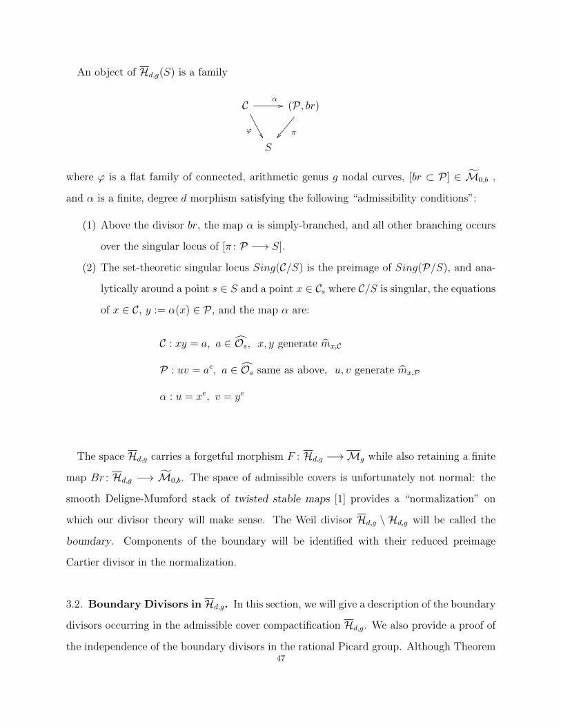
An object of Hd,g(S) is a family

Cα//

ϕ

(P , br)

π

S

where ϕ is a flat family of connected, arithmetic genus g nodal curves, [br ⊂ P ] ∈ M0,b ,

and α is a finite, degree d morphism satisfying the following “admissibility conditions”:

(1) Above the divisor br, the map α is simply-branched, and all other branching occurs

over the singular locus of [π : P −→ S].

(2) The set-theoretic singular locus Sing(C/S) is the preimage of Sing(P/S), and ana-

lytically around a point s ∈ S and a point x ∈ Cs where C/S is singular, the equations

of x ∈ C, y := α(x) ∈ P , and the map α are:

C : xy = a, a ∈ Os, x, y generate mx,C

P : uv = ae, a ∈ Os same as above, u, v generate mx,P

α : u = xe, v = ye

The space Hd,g carries a forgetful morphism F : Hd,g −→Mg while also retaining a finite

map Br : Hd,g −→ M0,b. The space of admissible covers is unfortunately not normal: the

smooth Deligne-Mumford stack of twisted stable maps [1] provides a “normalization” on

which our divisor theory will make sense. The Weil divisor Hd,g \ Hd,g will be called the

boundary. Components of the boundary will be identified with their reduced preimage

Cartier divisor in the normalization.

3.2. Boundary Divisors in Hd,g. In this section, we will give a description of the boundary

divisors occurring in the admissible cover compactification Hd,g. We also provide a proof of

the independence of the boundary divisors in the rational Picard group. Although Theorem47

1 is not very interesting in its own right, the strategy of exploiting the inductive structure

of the boundary may be of some interest to some readers. Roughly speaking, the difficulty

in working with the boundary divisors stems from 3 sources: (1) There are simply too many

boundary divisors, (2) for degrees d > 5, the construction of test families becomes nontrivial

due to a lack of “linear algebraic” parametrizations of Hurwitz space and (3) If one is to

use test families, one must somehow maintain control over the intersection of test families

with boundary divisors. We overcome these difficulties by “concentrating” issues (2) and (3)

into “genus 0” families, and “hyperelliptic” families. The reader will see precisely what this

means in Lemma 3.3.

Before carrying on, we will introduce a graph-theoretic representation of admissible covers

(and boundary divisors).

3.3. The decorated dual graph. Recall that the branch morphism Br : Hd,g −→ M0,b is

finite. This means that every boundary divisor E will lie over a unique boundary divisor,

Br(E) ⊂ M0,b. Therefore, the generic admissible cover [α : C −→ P] parametrized by E will

have a fixed branching profile which is the union of two marked P1’s: bL ⊂ P1L and bR ⊂ P1

R.

The curve P is simply P1L glued to P1

R at a point x which is not any of the branch points.

Furthermore, C breaks up into two halves CL and CR which are the preimages of P1L and

P1R. Since C is a nodal curve, it has a dual graph ΓC whose vertices v are marked by the

geometric genera gv of the corresponding components. We furthermore label every vertex as

either an L-vertex or an R-vertex depending on whether it parametrizes a component of CL

or CR respectively. Furthermore, we label every vertex v with its degree dv. Since the nodes

of C must lie over the node x, we see that every edge in ΓC must join an L-vertex with an

R-vertex. Finally, we label every edge e with the index of ramification re occurring at the

corresponding node. (The index of ramification of z → zm is m− 1)

We may arrange the vertices of the graph ΓE in two columns, the left, and the right

side. In this way, we may easily represent the boundary divisors by their decorated dual

graphs. One small detail is worth mentioning: The locus of covers with fixed dual graph48

is irreducible. This follows from the fact that the moduli space of branched covers of P1,

simply branched everywhere except perhaps at one point, is irreducible.

Labeling every vertex and edge of ΓE will often be notationally cumbersome and unnec-

essary. Therefore, we will adopt the following rule: Genus 0 vertices and unramified edges

will usually be left undecorated. Furthermore, we note that since the degree of a vertex v is

determined by all ramification indices of edges containing v, we need not specify both the

degrees and ramification indices.

For example, in H3,g, we may consider the boundary divisor E generically parametrizing

covers of the form:

vL, gL vR, gR

The corresponding dual graph ΓE would be:

•vLgL

•vRgR

•

2

3.4. Some more examples. We provide some examples for the reader’s convenience. These

examples are not selected randomly: they all lie above ∆2 ⊂ M0,b, i.e. two branch points

are colliding. In enumerative settings, the divisors lying over ∆2 ⊂ M0,b show up most

frequently, so we refer to them as the “enumeratively relevant” boundary divisors. For the

reader’s convenience, we indicate the dual graphs of 4 basic enumeratively relevant divisors.

(1) ∆irr, admissible covers having dual graph Γ∆irr:

•(d,g−1)•w

••

“left side” “right side”

...

49

(2) Tad, “triple ramification”. These are covers with dual graph ΓTad :

•(d,g)•••

3

...

(3) Dad, “stacked (2, 2) ramification”. These covers have dual graph ΓDad :

•(d,g)••

••

2

2

...

(4) Bad, “basepoint”. These covers have dual graph ΓB:

•(d−1,g)

• •••...

We will briefly explain the interpretation of Γ∆irr, just for the reader’s convenience. The

vertex w ∈ Γ∆irris unlabeled, so has genus 0. Furthermore, both edges emanating from w

are unramified, therefore the degree dw of w is 2. So the rational curve curve associated to

w is attached to the curve Cv at two points. The stable model is therefore an irreducible

nodal curve, hence the label “∆irr”.

Pick any boundary divisor D, and choose a general admissible cover [α : C −→ P ] ∈ D.

Let p ∈ P be the unique node, and let (d1, d2, ..., dk) be the local degrees of α occurring at

the nodes (q1, ..., qk) above n. The description of the versal deformation space Def α is given

in Harris-Mumford [14] as

∆b−4 × Spec k[[t1, t2, ..., tk, s]]/(td11 = td22 = ... = tdkk = s)

50

where ∆b−4 is a smooth germ. Above Def α, we have a versal family

C ⊂ Cα

//

ϕ !!

P ⊂ P

π

Def α

Locally around the node n ∈ P ⊂ P , P has local equation uv = s. At the nodes

qi ∈ C ⊂ C, i = 1, 2, ..., k, the total space C has local equation xiyi = ti.

This local description of the boundary allows us to understand intersection multiplicities.

In particular, we consider the following situation. Let F1

C1

α1//

P1

Tτ1

OO

σi

OO

be a family of d sheeted covers having k sections σi, i = 1, ..., k mapping to the marked

section τ1, where, around the section σi the map α1 has local degree di over τ1. Let F2 be

another family of the same type over the same base T :

C2

α2//

P2

Tτ2

OO

σi

OO

Suppose we glue the two families of covers along the sections σi and τ1,2 to obtain a family

of admissible covers

C1 ∪ C2

α1∪α2//

P1 ∪ P2

T

The admissibility condition tells us that

(Nσi/C1 ⊗Nσi/C2)⊗di = (Nσj/C1 ⊗Nσj/C2)

⊗dj = Nτ/P1 ⊗Nτ/P2

51

When we pass to the normalization of Hd,g, the family T will have intersection number

deg (Nτ/P1 ⊗Nτ/P2)/lcm(d1, ..., dk)

with the boundary divisor E in which it is contained. (We assume that T does not have

additional isolated intersections with E, in which case we must add these contributions

appropriately.) This follows from normalizing the local equations defining Def α.

From the local equations, we notice that the map Br : Hd,g −→M0,b is unramified along

a boundary divisor E exactly when the dual graph ΓE has no edges e with re > 0. In

other words, the general admissible cover parametrized by E has no ramification occurring

at the nodes. Therefore, we will call a boundary divisor E unramified if the generic admissi-

ble cover parametrized by E has no ramification occurring at the nodes. Otherwise, we will

call E a ramified divisor. Finally, if ΓE has exactly 2 vertices, we will call E a 2-vertex divisor.

3.5. Admissible Reduction. In this section, we explain the process of “admissible reduc-

tion”. The general problem is stated as follows: Suppose we have a family of degree d

covers

(3.1) Cα

//

ϕ

P1∆

π

∆ = Spec k[[t]]

where C is a family of generically smooth nodal curves (having smooth total space) mapping

d : 1 onto P1∆. In other words, we have a map t : ∆ −→ Hd,g, with the image of the punctured

disc ∆∗ lying in the interior Hd,g. How do we arrive at the corresponding family of admissible

covers?

3.5.1. Replacing a node. Suppose the central fiber C0 ⊂ C has a node x ∈ C0, and suppose

the local equation of C around x is uv − t. Let’s assume that x is the unique node of C0,52

just for simplicity - the general procedure is basically the same. In other words, the arc ∆

intersects the total boundary δ transversely at t = 0 along exactly one component.

We first make an order 2 base change Spec k[[s]] −→ Spec k[[t]] given by t → s2, and

consider the new family

C ′α′

//

ϕ′

P1∆′

π′~~

∆′ = Spec k[[s]]

We may consider the point x as living in C ′, where it is an A1 singularity of C ′. Let y :=

α(x) ∈ P1∆′ be the image. To arrive at a family of admissible covers, we blow up the point

y ∈ P1∆′ , the reduced point x ∈ C ′, and the d − 2 remaining points of α−1(y). The reader

can check that in this way we obtain an admissible cover [αad : Bl C ′ −→ Bl P1∆′ ] ∈ Hd,g(∆

′).

3.5.2. Replacing higher ramification. Now that we know how to replace nodes, we describe

how to replace higher ramification. Suppose

Cα

//

ϕ

P1∆

π

∆ = Spec k[[t]]

is a general family such that there exists a (unique, say) point x ∈ C0 ⊂ C such that the

finite cover α0 : C0 −→ P1 is locally given by z → ze where e ≥ 3. Let y := α(x) ∈ P1∆ We

first perform a base change Spec k[[s]] −→ Spec k[[t]] given by t → se−1 to arrive at the

pullback family as before:

C ′α′

//

ϕ′

P1∆′

π′~~

∆′ = Spec k[[s]]

We let Z ⊂ P1∆′ be the scheme theoretic preimage of y. Therefore Z ' Spec k[ε]/(εe−1).

We then blow up P1∆′ along Z and blow up C ′ at the reduced preimage of Z. The reader

53

can check that there is then a map αad : Bl C ′ −→ BlZ P1∆′ which provides the admissible

replacement.

Notice in both situations that a base change is always required. The reason why this is

true is that the branch morphism Br : Hd,g −→ M0,b is generically representable, and so we

need to, at the very least, extend the induced maps ∆∗ −→ M0,b, which generically requires

an order e−1 base change to separate the sheets of the e−1 branch points coming together.

The admissible reduction process allows us to understand the relationship between Hd,g

and Hd,g. There is a birational map R : Hd,g 99K Hd,g which extends in codimension one

over the enumeratively relevant boundary divisors. The admissible reduction process shows

that R∗(T ) = 2Tad, R∗(D) = 2Dad, and R∗(δirr) = 2∆irr. In fact, the pullback of any

component of the total boundary δ is twice the “corresponding” divisor in the admissible

cover compactification.

3.6. Independence of the boundary divisors. It appears as though the proof of inde-

pendence of boundary divisors is not easy to find in the existing literature. Therefore, we

provide a proof in this section. The reader is of course invited to skip this section. The main

point of interest, in the author’s opinion, is the choice of test families which will be used.

We take a moment to describe a class of test families which we call partial pencils.

3.7. Partial pencils. We now describe a method for constructing test families which have a

“controlled” intersection with boundary divisors. Consider the linear system of (m, d) curves

on P1 ×P1. Suppose we pick a distinct d -tuple of points Z lying entirely in a (1, 0) ruling

curve, which we call F . Consider a general linear pencil P1t ⊂ |(m, d)| of curves containing

Z in its base locus B. The total space of the pencil

p : X −→ P1t

is the blow up of P1 × P1 along B. Since we have forced d points of F to be in the base

locus, the pencil will be constant along F , so there will be some value , say t = 0, where the

fiber X0 of p splits off F as a component. In other words, there is a unique element of the54

pencil, X0 which is a union of F and a (m, d − 1) residual curve R. We may suppose that

X0 = F ∪R is general among such reducible curves.

The utility of the family p comes from the fact that the fixed locus Z provides d sections

σi along which we may attach “the rest” of an admissible cover. When we try to construct

families of admissible covers, we generally want to avoid the combinatorial analysis that

comes with “uncontrolled” incidences of branch points. Therefore, we prefer to use the

pencils as described above. Notice that whenever a ramification point approaches any of the

sections σi (i.e. points of Z), the entire fiber F is forced to split off, which will provide an

intersection with only one other boundary divisor which is easy to describe. The rest of the

pencil, i.e. away from t = 0, only provides intersections with enumeratively relevant divisors:

triple ramification, stacked (2, 2) ramification, and simple nodes may occur.

In the sequel, we will see other instances of similar families arising. The ambient surface

P1 ×P1 may be different (e.g. other Hirzebruch surfaces), but the general construction will

almost always be the same: We force the “maximal” number of base points in a “fiber”

forcing the fiber to split off. This gives us control over the divisors with which the resulting

family will interact. A family of admissible covers which is created from such a construction

(by, say, attaching a constant family at the sections σi) will be called a partial pencil family.

(The name comes from thinking about the family as a pencil, but only varying “one half” of

an admissible cover.)

Theorem 3.1. The boundary divisors are independent in PicQHν

d,g for g ≥ 3.

Proof. We will use the method of test families. Begin with a dependence relation

0 =∑E

c(E) · E

Let us rewrite the dependence relation as:55

(3.2) aλ+ bδ + cD +∑E′

c(E ′) · E ′ +∑E

c(E) · E = 0

where the first sum is over all enumeratively relevant divisors other than Tad, Dad, and

∆irr. We will call the coefficients c(E ′), along with a, b, and c the enumeratively relevant

coefficients. The second sum is over all other boundary divisors, and the divisors classes λ

and δ are pulled back via the forgetful morphism F : Hd,g −→ Mg. We may perform this

change of basis thanks to Proposition 1.4. The first claim is that the coefficients c(E) are

linear combinations of a, b, c and the c(E ′). Before proving this reduction, we will need a

definition. Define the excess, ex(E), of a boundary divisor E to be

(3.3) ex(E) := min ∑L−vertices

gv + rv,∑

R−vertices

gv + rv

.

Therefore, the divisors with ex(E) = 0 are precisely those which are unramified and have

only rational components on one side.

Lemma 3.2. If ex(E) = 0, then the coefficient c(E) is a linear combination of the enumer-

atively relevant coefficients.

Proof. Pick a rational vertex v ∈ ΓE which has degree dv ≥ 2. Vary v in a pencil of (1, dv)

curves on P1 × P1, with dv distinct basepoints forced to lie in a (1, 0) fiber. The resulting

test family γ has negative intersection with E and has 0 intersection with λ. Otherwise, the

test family γ intersects D, δ, and perhaps some other enumeratively relevant divisors, but

no others. Therefore, we obtain a relation among c(E), c(E ′), a, b, and c, which is what we

wanted.

Before continuing on with the proof of the theorem, we will introduce a useful construction

of test families which will help us “reduce” the ramification occurring above a node. On

P1×P1, consider a pencil P1t of (1, d) curves such that the base locus contains a Spec k[ε]/(εd)

56

subscheme of a (1, 0) ruling line. Suppose P1t is general among such pencils. Let

p : X −→ P1t

be the total space of the pencil. X will have exactly one Ad−1 singular point s ∈ X which will

be a singular point of the corresponding fiber X0 of p. The curve X0 has two components S0

and T0, where S0 is a (0, 1) curve and T0 is a (1, d− 1) curve. The two components intersect

transversally at the reduction of the k[ε]/(εd) point in the base locus, and T0 contains a

Spec k[ε]/(εd−1) subscheme of Spec k[ε]/(εd), i.e. is totally ramified under the projection to

the first factor.

The family p : X −→ P1t has a section σ corresponding to the reduced basepoint underlying

Spec k[ε]/(εd). The singular point s ∈ X is contained in this section σ. If we partially blow

up the point s, we arrive at a family p : X −→ P1t with an Ad−2 singular point s ∈ X, and a

new central fiber X0 = S0 ∪ T0 ∪ P , where P ' P1 is the exceptional divisor of the blow up.

The singular point s is precisely S0 ∩ P . Furthermore, the section σ now passes through a

general point of P . (We are considering strict transforms everywhere.)

The rational component P has a well defined pencil of degree d on it. Indeed, set x := σ∩P ,

y := P ∩ S0, and z := P ∩ T0. Then the divisors d · x and y + (d− 1) · z span a well-defined

pencil of degree d on P .

Notice that the degree d map on P is ramified maximally at the point x (which will

eventually serve as a point of attachment with the rest of an admissible cover) and ramified

to order d − 1 at the point z. Furthermore, all other elements of the pencil p are totally

ramified along the section σ. Therefore, the family p : X −→ P1t will serve (perhaps after

some finite base changes) as a “ramification reducing” test family, as we see in the next

lemma.

Lemma 3.3. Let E have excess ex(E) = n > 0. Then c(E) is a linear combination of the

enumeratively relevant coefficients and one more coefficient, c(Ei), where ex(Ei) < n.57

Proof. If the divisor E is unramified, pick a vertex v ∈ ΓE (on the side with smaller sum of

genera) of genus gv > 0. Suppose the dual graph, locally around v, had the following form:

•...

...

...

...

...

v

(dv ,gv)

We will now “concentrate” all of the genus of the vertex v into a hyperelliptic vertex, which

allows us to vary the vertex in a family. So, we will replace this part of the dual graph with

the following picture.

•

•

••

•v′

gv′=gvdv′=2

...

...

...

...

...

w

dw=dv−1, gw=0

Now we vary the genus gv hyperelliptic curve v′ in a pencil of |2τ + f | curves on Fgv ,

with two pairs of prescribed basepoints lying in two chosen fibers of the natural projection

π : Fgv −→ P1. The resulting test family γ provides the reduction we seek because it has

nonzero intersection with E and with two higher boundary divisors with strictly smaller

excess.

If the divisor E is ramified, we concentrate our attention at a vertex v, such that locally

around v the dual graph has the form:

•...

...

...

...

...

v

(dv ,gv)

m

58

(The top edge in the diagram has ramification index m.) We replace this local picture with:

•••

••...•

•v′

gv′=0

dv′=m+1

•w′

gw′=gv

dw′=dv−(m+1)

...

.........

...

m

We vary the totally ramified, degree m + 1 rational vertex v′ in P1 × P1 with an (m + 1)-

fold basepoint fixed in a fiber. The resulting test family will intersect E negatively, and

will intersect other higher boundary divisors which have strictly smaller total ramification

index.

Finally, we show that the enumeratively relevant coefficients are zero.

Lemma 3.4. The enumeratively relevant coefficients are zero.

Proof. We will argue by reducing the degree d incrementally. First we note that using partial

pencil families like those in section 4.4 we may easily deduce Lemma 3 when d = 3 and d = 4.

(In fact, we can also show it for d = 5, but we don’t need this.) Therefore, we assume d ≥ 5.

Furthermore, we must assume g ≥ 3 because there is a relation between λ and δ when g ≤ 2

which persists in Hurwitz space.

We switch to the partial compactification Hd,g (which is compact in codimension 1) where

we deduce from relation (1) the relation aλ+ bδ+ cD+∑c(δ′) · δ′ = 0 in PicQ Hd,g. We may

do this because, as we have seen, one only needs to make an order two base change to pass

from a family T ⊂ Hd,g to a family of admissible covers. Therefore, the relation remains the

same, up to multiplication by 2. Here we are writing δ′ to refer to the remaining boundary

divisors. Among the divisors δ′ is the divisor B parametrizing “covers with a basepoint”. A

general cover [α : C −→ P1] ∈ B has a singular domain curve C = L ∪ C ′ where L ' P1

maps isomorphically to P1 under α, C ′ is a genus g, degree d − 1 cover of P1, and L ∩ C ′

is one point, which we call the “basepoint”. The coefficient c(B) is easily seen to be 0:

Consider the family S obtained by “sliding” the basepoint along C ′. This family intersects59

B negatively, and has trivial intersection number with λ, δ, and D, and all other boundary

divisors.

Now consider a general complete curve T ⊂ Hd−1,g obtained from a family

(3.4) Cα//

f

P

g

T

After a suitable base change (which may be performed globally over Hd−1,g) we may assume

that the family f has a section s satisfying s2 6= 0. We attach a constant “basepoint”

P1 to the family f along s to obtain a family T ′ ⊂ B ⊂ H′d,g. The relation (2) then

implies the same for the family T ⊂ Hd−1,g. Since we would obtain relation (2) for any

complete curve T ⊂ Hd−1,g avoiding a codimension 2 locus (where the section intersects

triple ramification points for example), we would deduce that the relation (3.2) must also

hold in PicQ Hd−1,g.

The independence of the boundary now follows from Lemmas 1, 2, and 3.

Remark 3.5. Another way to phrase the argument in Lemma 3 is: The boundary divisor B

parametrizing “basepoints” is birational to the universal genus g curve over Hd−1,g. Thus, by

restricting relation (3.2) to B, we obtain a relation on Hd−1,g, which has the same coefficients

as the original relation.

60

4. Enumerative Geometry

After describing the relationships between various “natural” divisor classes on Hurwitz

spaces, we will go on to describe the divisor classes of the Maroni and Casnati-Ekedahl di-

visors. These descriptions will then allow us to determine sharp upper bounds for slopes of

sweeping families of trigonal, tetragonal, and pentagonal curves, extending the Cornalba-

Harris bound for hyperellitpic curves, and Stankova’s bound for trigonal curves. All inter-

sections will be considered as occurring on the appropriate Deligne-Mumford stack.

4.1. The natural divisor classes on Hd,g. Let’s consider the universal smooth d sheeted

cover of genus g:

Cu

//

ϕ

P

π

Hd,g

On the P1-bundle P , we have the universal reduced direct image Eu and bundle of quadrics

Fu. In Hd,g, we have the following divisor classes:

(1) λ, pulled back from Mg.

(2) δ, the total boundary pulled back from Mg.

(3) T , the locus of branched covers which have a triple ramification point.

(4) D, the locus of branched covers which have stacked (2, 2) ramification somewhere.

(5) π∗(c21Eu)

(6) π∗(c2Eu)

(7) π∗(c21Fu)

(8) π∗(c2Fu)

(9) ϕ∗(c21(ωu))

(10) ϕ∗(c1(ωu) · u∗c1(ωπ))

(The divisor class ϕ∗(u∗c2

1(ωπ)) is 0 because π is a P1-bundle.) We will call these 10 classes

the natural divisor classes on Hd,g.61

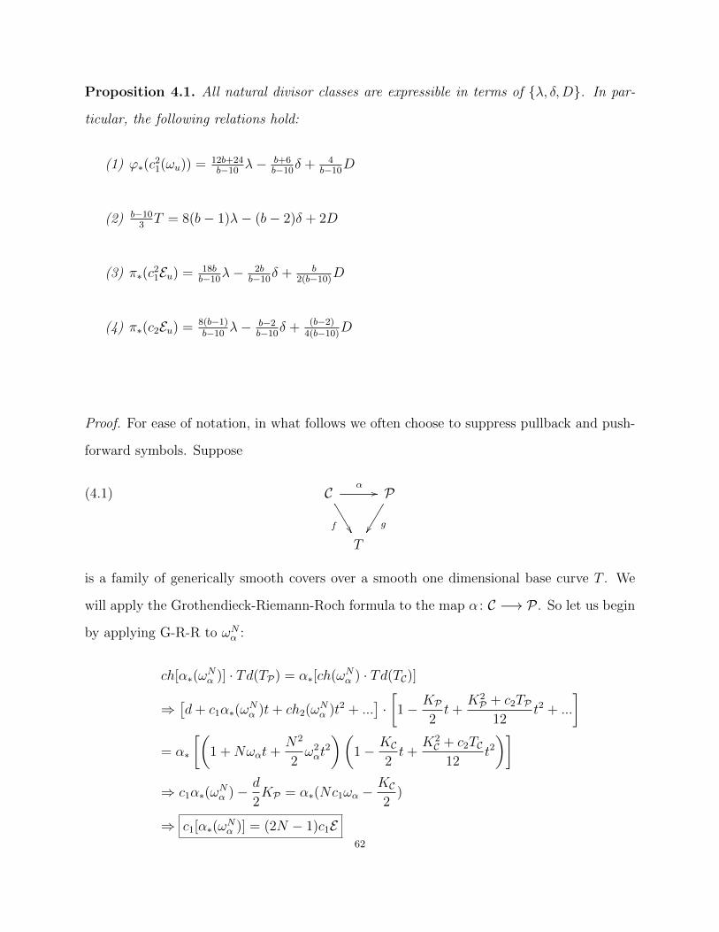
Proposition 4.1. All natural divisor classes are expressible in terms of λ, δ,D. In par-

ticular, the following relations hold:

(1) ϕ∗(c21(ωu)) = 12b+24

b−10λ− b+6

b−10δ + 4

b−10D

(2) b−103T = 8(b− 1)λ− (b− 2)δ + 2D

(3) π∗(c21Eu) = 18b

b−10λ− 2b

b−10δ + b

2(b−10)D

(4) π∗(c2Eu) = 8(b−1)b−10

λ− b−2b−10

δ + (b−2)4(b−10)

D

Proof. For ease of notation, in what follows we often choose to suppress pullback and push-

forward symbols. Suppose

(4.1) Cα//

f

P

g

T

is a family of generically smooth covers over a smooth one dimensional base curve T . We

will apply the Grothendieck-Riemann-Roch formula to the map α : C −→ P . So let us begin

by applying G-R-R to ωNα :

ch[α∗(ωNα )] · Td(TP) = α∗[ch(ωNα ) · Td(TC)]

⇒[d+ c1α∗(ω

Nα )t+ ch2(ωNα )t2 + ...

]·[1− KP

2t+

K2P + c2TP

12t2 + ...

]= α∗

[(1 +Nωαt+

N2

2ω2αt

2

)(1− KC

2t+

K2C + c2TC

12t2)]

⇒ c1α∗(ωNα )− d

2KP = α∗(Nc1ωα −

KC2

)

⇒ c1[α∗(ωNα )] = (2N − 1)c1E

62

Note: From the exact sequence

0→ F → S2E → α∗(ω2α)→ 0

we immediately deduce the conjecture stated in Casnati’s hexagonal covers paper:

F = (d− 3)c1E

If we consider the degree 2 part in the G-R-R calculation, we arrive at the relation:

[ch(α∗(ωNα ))]2 = [chE ]2 +

(N2

)c2

1(ωα)

In particular, we notice that [chF ]2 is expressible in terms of [chE ]2 and c21(ωα), and therefore

c2F is expressible in terms of [chE ]2,c21(ωα), and c2

1E .

By applying G-R-R to f , we see

λ = χ(OC)− χ(OT )χ(OCη)

where Cη where denotes the generic fiber of f . Applying G-R-R to α as before, we can show:

λ =

(1

2− 1

b

)c2

1(E)− c2(E)

Where b = 2d+ 2g − 2, the number of branch points.

We now compute κ. By definition, κ = ω2f = (ωα +α∗(ωg))

2 = ω2α + 2(ωα ·α∗ωg). Now, we

know thatc21(E)

b= c1E ·

[−ωg2

], and that α∗c1ωα = 2c1E = B, the class of the branch divisor.

Combining this information gives:

κ = ω2α −

8c21(E)

b

63

Mumford’s relation [19] δ = 12λ− κ gives:

δ = 12

(c2

1(E)

2− c2(E)− c2

1(E)

b

)−(ω2α −

8c21(E)

b

)=

(6− 4

b

)c2

1E − 12c2E − ω2α

In order to understand the divisors D and T , we use the double point formula for the

ramification divisor R := c1(ωα) of α mapping onto the branch divisor B ⊂ P . (Equiva-

lently, we interpret simple cusps and nodes occurring in B as intersections with T and D,

respectively.)

Adjunction, both on C and P , gives the following:

2pa(R)− 2 = ωα · (ωα +KC) = ωα · (2ωα + α∗KP)

2pa(B)− 2 = B · (B +KP)

=⇒ pa(B)− pa(R) =B2

2− ω2

α = 2c21(E)− ω2

α = T +D

Next, note that the ramification of f : R→ T gives the number T + δ:

T + δ = ωα · (ωα + ωf ) = ωα · (2ωα + α∗ωg) = 2ω2α + ωα · α∗ωg = 2ω2

α −4c2

1(E)

b

Solving for T , and using the expressions above gives

T = 3ω2α − 12

(c2

1(E)

2− c2(E)

)(4.2)

D = 8c21(E)− 12c2(E)− 4ω2

α(4.3)64

After manipulating the various relations above, we arrive at the following:

ω2α =

12b+ 24

b− 10λ− b+ 6

b− 10δ +

4

b− 10D(4.4)

b− 10

3T = 8(b− 1)λ− (b− 2)δ + 2D(4.5)

c21(E) =

18b

b− 10λ− 2b

b− 10δ +

b

2(b− 10)D(4.6)

c2(E) =8(b− 1)

b− 10λ− b− 2

b− 10δ +

(b− 2)

4(b− 10)D(4.7)

(chE)2 =b+ 8

b− 10λ− 2

b− 10δ +

1

2(b− 10)D(4.8)

Remark 4.2. Note that we have shown that c1F = (d− 3)c1E . The proof was not specific to

our situation, so the conjecture appearing in [5] is settled. In fact, it follows that all chern

classes of the higher syzygy bundles Ni are expressible in terms of chern classes of E and F .

4.1.1. The divisor classes M and CE. We may now express the divisors M and CE in terms

of λ, δ, and D. Since π : P −→ Hd,g is a P1-bundle, we may use the Bogomolov expressions

for Eu and Fu, respectively, to find our expressions. For a rank r locally free sheaf G on P ,

the Bogomolov expression for G is

Bog(G) := c2G −(r − 1)

2rc2

1G

(It is, up to scaling, the unique linear combination of c2 and c21 which is invariant under

tensoring by pullbacks of line bundles from the base.) The Bogomolov expression detects

the change of splitting type of G on the fibers of the P1-bundle P [2]. Using Proposition 4.1,

we conclude:

65

Proposition 4.3. In PicQ Hd,g, the divisors M and CE are expressible in terms of λ, δ, and

D. These expressions are:

M =

(10−dd−1

b−8

b−10

)λ−

( 1d−1

b−2

b−10

)δ +

( 1d−1

b−2

4(b−10)

)D

CE =(

(21−d− 54d

)b−8d+24

b−10

)λ−

((2− 6

d)b−2d+6

b−10

)δ +

((1− 6

d)b−2d+16

4(b−10)

)D

Proof.

Remark 4.4. By an earlier remark, the Bogomolov expressions for every syzygy bundle Ni

are expressible in terms of λ, δ, and D. This is to be expected if we believe the Picard Rank

Conjecture. We will explore the possible implications of this observation in the last section.

4.2. Slope bounds. Suppose we are given a family of stable genus g ≥ 2 curves f : C −→ T ,

where T is a smooth, complete curve. One way to measure the topological complexity of the

fibration is to count the number of singular fibers occurring in the family. This can be done

by considering the quantity

χtop(C)− χtop(Cη)χtop(T )

which will give the intersection number δ · T . (Cη denotes the general fiber.) This quantity

is zero precisely when the family T parametrizes smooth curves.

On the other hand, one way to measure the change in “moduli” is to consider the difference

χ(OC)− χ(OCη)χ(OT )

which, by a Grothendieck-Riemann-Roch calculation turns out to be λ · T .

One measure of the complexity by which the curve T rests inside Mg is simply the ratio

of the two quantities, or the slope:

s(T ) :=δ · Tλ · T

For example, the (projective) Satake compactification ofMg adds a codimension 2 boundary

and thereforeMg is swept out by complete curves T which, obviously, have slope 0. On the66

other hand, the Mumford relation [19]

12λ = δ + κ

and the fact that κ is positive [?] together imply that the slope is bounded above by 12.

Whereas it is easy, theoretically, to prove the existence of many families having slope 0,

one quickly realizes that families with higher slopes are more “special.” This is made more

precise by the following theorem of Cornalba and Harris [7]:

Theorem 4.5 (Cornalba, Harris [7]). Let f : C −→ T be a generically smooth family of

stable curves. Then the slope is bounded above by

s(T ) ≤ 8 +4

g

Furthermore, equality is achieved if and only if T is a family of hyperelliptic curves.

In other words, the maximal slope is achieved for families which are entirely contained in

some proper subvariety ofMg, namely the hyperelliptic locus. Furthermore, it is easy to see

that the hyperelliptic locus is actually swept out by families of slope 8+4/g, i.e. there exists

a curve T in the hyperelliptic locus whose algebraic deformations pass through the general

point of the hyperelliptic locus.

One way to understand the relationship slopes of families and special subvarieties of X ⊂

Mg is to ask the “reverse” question. Given a subvariety X ⊂ Mg, what is the maximum

slope of a sweeping curve T ⊂ X?

Taking the result of Cornalba and Harris as a starting point, one may ask the general

question for the locus of d-gonal curves Td ⊂ Mg. In Stankova’s thesis [22], the following

theorem was proved:

Theorem 4.6 (Stankova [22]). Let g ≥ 4 be even. For a sweeping curve T ⊂ T3,

s(T ) ≤ 7 +6

g67

In this section, we will extend Stankova’s results by establishing sharp upper bounds for

slopes of sweeping curves T in T4 and T5. The divisors M and CE will play an essential role.

In particular, our slope bounds will only hold under the appropriate congruence conditions

which must be met in order for M and CE to both exist as effective divisors.

After examining the expressions in Proposition 4.3, we observe that when d ≤ 5, the

coefficient of the boundary divisor D is positive in M, and negative in CE. Consider the

(unique, up to scaling) effective combination X of M and CE which eliminates the coefficient

of D,and write it as

X := aλ− bδ

If we think of X as an effective divisor in Hd,g (by taking the closure), we may include the

higher boundary divisors in the divisor class expression for X by writing

X = aλ− bδ −Y

Where Y is some combination of higher boundary divisors. Finally, observe that if Y is an

effective combination of higher boundary divisors, then the ratio ab

will be an upper bound

for the slope of a sweeping curve T ⊂ Hd,g. Fortunately, we have:

Theorem 4.7. Y is an effective combination of higher boundary divisors.

As corollaries of Theorem 4.7, we conclude:

Corollary 4.8 (Slope bounds for trigonal curves). If T ⊂ H3,g is a sweeping curve, and g

is even, then the slope s(T ) is bounded above by 21g+183g

. Furthermore, this bound is sharp.

Corollary 4.8 is Stankova’s result.

Corollary 4.9 (Slope bounds for tetragonal curves). If T ⊂ H4,g is a sweeping curve, and

if g ≡ 3 mod 6, then the slope s(T ) is bounded above by 26g+304g

. Furthermore, this bound is

sharp.

68

Corollary 4.10 (Slope bounds for pentagonal curves). If T ⊂ H5,g is a sweeping curve, and

if g ≡ 16 mod 20, then the slope s(T ) is bounded above by 31g+445g

. Furthermore, this bound

is sharp.

We have written the slope bounds in nonreduced form because by doing so, a definite

pattern emerges. If we include the original Cornalba-Harris bound 16g+82g

for slopes of hyper-

elliptic families, the pattern is further reinforced. Therefore, we make the conjecture:

Conjecture 4.11. When both M and CE exist as effective divisors in Hd,g, the slope of a

sweeping curve T ⊂ Hd,g is bounded above by

sconj =(5d+ 6)g + d2 + 5d− 6

dg

Further evidence for Conjecture 4.11 will be provided in the last section.

One interesting observation should be made regarding these slopes. [14] The canonical

class KMgis [14]:

KMg= 13λ− 2δ

The results above tell us that both the trigonal locus T3 and the tetragonal locus T4 are swept

out by KMg-negative curves. However, the locus T5 is not swept out by KMg

-negative curves.

This may be of some interest in the program of understanding the birational geometry of

Mg.

We will prove Theorem 4.7 for each degree d = 3, 4, 5 separately, beginning with d = 3. The

reader should note that all three arguments are inductive in nature: We carefully choose test

families which allow us to deduce the nonnegativity of certain coefficients in Y by knowing

the nonnegativity of other coefficients.

Since we are only trying to show effectivity of Y, we will not try to calculate the exact

class of Y. To see an exact description of the class of M in H3,g, we refer the reader to [9].

Before we begin with the proofs, we want to mention that it is not enough to show that

the enumeratively relevant boundary divisors have nonnegative coefficients. In other words,

we may not restrict ourselves to sweeping families of complete curves in Hd,g, because there69

may be sweeping families in the d-gonal locus Td which pass through a point lying outside of

the image of the nonproper forgetful map F : Hd,g −→Mg. This is why we must deal with

the monstrous boundary of the admissible cover compactification.

4.3. Slope bounds: d = 3. When the degree is 3 and the genus is even, the effective divisor

class

X := aλ− bδ −Y

is simply a multiple of the Maroni divisor M. Furthermore, the reader can check that

a = 7g + 6 and b = g.

For a boundary divisor E ⊂ Hd,g, we will denote by c(E,Y) the coefficient of E in the

divisor class expression of Y. We wish to show that c(E,Y) ≥ 0 for all higher boundary

divisors E.

Rather than create names for every boundary divisor, we will adopt the following simpli-

fying naming scheme: The letter E will always be understood to mean the divisor which

is “currently” of primary concern. All decorations on the letter E, (e.g. E ′, E1, etc.) will

indicate auxiliary boundary divisors occurring in the analysis of c(E,Y). Every section will

be devoted to showing c(E,Y) ≥ 0 for a specified type of boundary divisor.

We begin by considering unramified, 2-vertex divisors.

4.3.1. Unramified, 2-vertex Divisors. Let E have dual graph ΓE:

•vLgL

•vRgR

We let gR, gL denote the genus of the components vR, and vL. Furthermore, by symmetry

we may assume that gR ≤ gL. We will vary the right side in a partial pencil family. Consider

a pencil P1t of genus gR trigonal curves on F0 or F1 (depending on the parity of gR) with

three points p1, p2, p3 of the base locus lying on a fiber F0. After performing the admissible

reduction procedure to the pencil, and then attaching a constant family on the left, we arrive70

at a family of admissible covers γ which has the following intersection numbers:

λ · γ = 2gR

δ · γ = 2(7gR + 3)

E · γ = −2

E ′ · γ = 2

X · γ ≥ 0

Here, E ′ is the boundary divisor which has dual graph ΓE′ :

•v′LgL+2

•v′R

gR−2

Notice that we have simply decreased the genus of the right side by two. This was the reason

we impose the “collinear” basepoints. The fact that X · γ ≥ 0 follows from the observation

that the families of type γ sweep out the divisor E. (In fact, it can be shown that X · γ = 0,

but we do not need this.) The test family γ provides the relation:

(4.9) c(E,M) ≥ c(E ′,M) + 3g − 6gR

Since we are assuming that gR ≤ gL, and since gL + gR + 2 = g, we immediately conclude

that c(E ′,Y) ≥ 0 implies c(E,Y) ≥ 0. Suppose gR was even. Then by repeatedly applying

relation (4.9), we may conclude by showing that c(E0,Y) ≥ 0 for the boundary divisor E0

which has the dual graph ΓE0 :

•vL

g−2•vR

0

We use the same type of pencil as was used to construct γ above. Fortunately, the split

fiber does not contribute any intersection with further boundary components, because the71

residual curve R0 is a disjoint union of (1, 0) curves which will be blown down. Therefore, the

resulting partial pencil family of admissible covers, γ0 has the following intersection numbers:

λ · γ0 = 0

δ · γ0 = 6

E0 · γ0 = −2

X · γ0 = 0

From these calculations we easily see that c(E0,Y) ≥ 0, and this implies c(E,Y) ≥ 0.

The analysis for gR is completely analogous. We simply need to show that c(E1,Y) ≥ 0

where E1 has an elliptic curve as the right hand component. Again, we just use a partial

pencil family.

4.3.2. Simply Ramified 2-vertex divisors. Let E, a simply ramified 2-vertex divisor, have

dual graph ΓE:

•vLgL

•vRgR2

As before, we let gR, gL denote the genera of vR, vL and assume that gR ≤ gL. Vary vR in

a pencil P1t of genus gR trigonal curves in F0 or F1. This time, however, we impose the

condition that the base locus of our pencil contains a nonreduced “triple” 2p1, p2 of points

in a fiber F0.

The total space p : Ct −→ P1t of the pencil has a unique A1 singular point s occurring

above a point x ∈ P1t , and a split element F0 ∪ R0 occurring at, say, t = 0. The fiber of

Cx := p−1(x) is a nodal curve which is singular exactly at the point s. Furthermore, there

are two sections s1, s2 corresponding to the points p1 and p2. After resolving the singularity

s and blowing up s2 ∩ Cx, we arrive at a new family p : Ct −→ P1t , which has two sections

s1, s2, the strict transforms of s1 and s2. We note that s21 = −1.

After an order two base change (as usual in the admissible reduction process) we may

attach a “constant” genus gL trigonal curve [αL : CL −→ P1L] at the sections s1 and s2 to

72

obtain our test family γ of admissible covers. Obviously, we must attach a simple ramification

point of αL to the section s1. Notice that γ intersects two higher boundary divisors other

than E. The split element provides an intersection with the unramified boundary divisor E ′

which has dual graph ΓE′ :

•v′LgL+1

•v′R

gR−2

The fiber corresponding to the point x provides an intersection with the unramified boundary

divisor E ′′ which has dual graph ΓE′′ :

•v′′LgL

•v′′R

gR−1

The intersection numbers of γ are as follows:

λ · γ = 2gR

δ · γ = 2(7gR + 4)

E · γ = −2

E ′ · γ = 2

E ′′ · γ = 2

X · γ ≥ 0

This provides us with the relation

(4.10) c(E,Y) ≥ c(E ′,Y) + c(E ′′,Y) + 4g − 6gR

We already know from the previous section that c(E ′,Y) ≥ 0 and c(E ′′,Y) ≥ 0. Further-

more. we are assuming gR ≤ gL. Therefore c(E,Y) ≥ 0.73

4.3.3. Triply ramified 2-vertex divisors. Now let E be a triply ramified, 2-vertex divisor with

dual graph ΓE:

•vLgL

•vRgR3

Once again, we begin by varying vR in a pencil on the appropriate Hirzebruch surface (F0

or F1 depending on the parity of gR.) We impose a triple point “3p1” (isomorphic to

Spec k[ε]/(ε3)) in a fiber F0 to be contained in the base locus of the pencil. We arrive

at a total space p : Ct −→ P1t which has a unique A2 singularity s occurring in the fiber

Cx := p−1(x), for some x ∈ P1t . Furthermore, the nodal curve Cx is not only singular at the

point s, but is also simply tangent to the fiber F0 along one of its branches. The base point

p1 provides a section s1, and as usual we have a split element F0 ∪R0 at t = 0.

Consider the resolution of s, p : Ct −→ P1t . The fiber p−1(x) is now Cx ∪ E1 ∪ E2, where

E1 ∪ E2 is the chain of exceptional divisors coming from resolving an A2 singularity, and

Cx is the normalization of Cx. Cx intersects E1 at a point a and E2 at the point b. Let’s

assume that a corresponds to the ramified branch of Cx. Then the strict transform of the

section, which we will continue to call s1, has self intersection −1, and passes through the

exceptional divisor E1.

Now blow down E2 to acquire a family p′ : C ′t −→ P1t . The fiber p′−1(x) is now the union

Cx ∪ E1, where Cx ∩ E1 = a, b. The total space C ′t has an A1 singularity at the point

b. After an order two base change (admissible reduction), we may glue a constant, triply

ramified trigonal curve αL : CL −→ P1L to p′ along the section s1, to obtain our family γ of

admissible covers. The split fiber of γ provides an intersection with the unramified boundary

divisor E ′ with dual graph ΓE′ :

•v′LgL

•v′R

gR−2

74

The fiber corresponding to the point x provides an intersection with the simply ramified

boundary divisor E ′′ which has dual graph ΓE′′ :

•v′′LgL

•v′′R

gR−12

The intersection numbers for γ are now:

λ · γ = 2gR

δ · γ = 2(7gR + 5)

E · γ = −2

E ′ · γ = 2

E ′′ · γ = 2

X · γ ≥ 0

As a result, we obtain the relation

(4.11) c(E,Y) ≥ c(E ′,Y) + c(E ′′,Y) + 6g − 5gR

From this relation we conclude c(E,Y) ≥ 0.

4.3.4. More than 2 vertices. Now let’s suppose E has a dual graph with more than 2 vertices.

Then one of the vertices, vR, must have degree 2, i.e. it must correspond to a hyperelliptic

component. Let us assume ΓE is:

•gL

vL •vRgR•

75

A priori, there are two types of 3-vertex divisors: Either vR is ramified, or not. (We will

only consider the analysis for the unramified case - the reader will by now be able to make

the necessary minor adjustments for the ramified case.)

We vary the genus gR hyperelliptic curve vR in a P1t pencil on FgR+1 with two specified

points p1, p2 in a fiber F0 lying in the base locus. The resulting family of admissible covers,

γ, will intersect a new boundary divisor E ′ which has dual graph ΓE′ :

•gL+1

v′L •v′R

gR−1•

(Notice that we are simply reducing the genus of vR by one.) The intersection numbers for

γ are:

λ · γ = 2gR

δ · γ = 2(8gR + 2)

E · γ = −2

E ′ · γ = 2

X · γ ≥ 0

We end up with the relation

(4.12) c(E,Y) ≥ g(gR + 2)− 6gR + c(E ′,Y)

The expression g(gR+2)−6gR is always non-negative for 0 ≤ gR ≤ g−1, g ≥ 2. Therefore,

if c(E ′,Y) ≥ 0, then c(E,Y) ≥ 0. By repeatedly use relation (4.12), we must only show76

that c(E0,Y) ≥ 0 for E0 having dual graph ΓE0 :

•g−1

vL •vR0•

But notice E0 is just ∆irr, and clearly c(∆irr,Y) = 0, so we are done.

4.3.5. 4 vertices. Now suppose the dual graph for E looks like ΓE:

•gL

vL

• •vRgR•

As usual, assume that gR ≤ gL. Again, vary vR in a partial pencil of hyperelliptic curves.

We obtain a family of admissible covers γ which intersects one other higher boundary divisor

E ′ whose dual graph is ΓE′ :

•gL

v′L •v′R

gR−1•

In other words, E ′ is of the type discussed in the previous subsection - the left sides of the

admissible covers represented by E ′ have only one vertex. The intersection numbers for γ

are:

λ · γ = 2gR

δ · γ = 2(8gR + 3)

E · γ = −2

E ′ · γ = 2

X · γ ≥ 0

Therefore, we arrive at the relation:

(4.13) c(E,Y) ≥ g(gR + 3)− 6gR + c(E ′,Y)77

For all acceptable pairs (gR, g), the expression g(gR + 3) − 6gR is easily checked to be

nonnegative, so we conclude that c(E,Y) ≥ 0.

This concludes the proof of Stankova’s theorem for H3,g, g even.

4.4. Slope bounds: d = 4. The proof of Theorem 4.7 for H4,g runs almost exactly as

the proof of the d = 3 case. After seeing the general inductive method in the previous

section, we pause to notice a few things. First, the underlying pencil used to construct the

appropriate test families obviously depended on the degree of the vertex vR which was being

varied: pencils of trigonal curves in F0 or F1 for degree 3 vertices, and pencils of genus

gR hyperelliptic curves in FgR+1 for degree 2 vertices. When we switched to considering

hyperelliptic pencils, the quantity bδ − aλ becomes “much more positive” than it is when

we consider pencils of trigonal curves. This essentially happens because the slope 8gR+4gR

of a

hyperelliptic family is larger than ab

= 7g+6g

.

Now that we are considering the degree 4 situation, we notice that a similar phenomenon

occurs. For a divisor E whose dual graph has more than 2 vertices, we may use the same

types of pencils used in the previous case: either pencils of trigonal curves in F0,1, or pencils

of hyperelliptic curves of genus gR in FgR+1. Because ab

= 13g+152g

is fundamentally smaller

than 7gR+6gR

and 8gR+4gR

, arguments exactly like those found in the previous section show that

c(E,Y) ≥ 0 if we know positivity for “low genus” examples of such E. The low genus cases

are easy to establish, so we will leave them to the reader.

Therefore, it is the 2-vertex boundary divisors which are of primary interest. We will need

to exhibit fundamentally new partial pencil families, heavily relying on the description of

degree 4 covers as complete intersections in their associated scrolls.

4.4.1. Constructing sweeping families of tetragonal curves. Recall that a tetragonal, genus

gR cover [α : C −→ P1] rests in its associated scroll π : PE −→ P1 as a complete intersection

of two relative conic divisors Qu and Qv in the linear systems |2ζ − uf | and |2ζ − vf |,

respectively. The integers u and v are such that Fα = O(u)⊕O(v). Let us assume, as usual,78

that u ≤ v, so that v = dgR+32e. The line bundle O(2ζ − vf) is always globally generated on

PE , while O(2ζ − uf) is always very ample.

We fix a smooth element S ∈ |2ζ − vf |, and consider a pencil P1t ⊂ |2ζ − uf | on S. Let

p : S −→ P1t denote the total space of the pencil. So p is a family of tetragonal curves, and

S is just the blow up of S at the base locus of the pencil. We compute the invariants δp and

λp using standard methods.

The Euler characteristic, χ(OS) = 1, so

λp = χ(OS)− χ(OP1t)χ(OCgen) = gR

where Cgen denotes the curve in the pencil.

To compute δp, we do the following. Letting L := OS(2ζ − uf), we recall that:

δp = c2(L+ L⊗ ΩS) = c1(L) · c1(L⊗ ΩS) + c2(L⊗ ΩS)

= c1(L)[KS + 2c1(L)] + c2(L⊗ ΩS)

= c1(L)[KS + 2c1(L)] + c2(ΩS) + c1(L)KS + c21(L)

= 3c21(L) + 2c1(L) ·KS + c2(ΩS)

= 2(2gR − 2) + c21(L) + c2(ΩS)

To compute c21(L), we just intersect

c21(L) = (2ζ − uf)2(2ζ − vf) = [4ζ2 − 4uζf ][2ζ − vf ]

= 8ζ3 − 8u− 4v = 8(u+ v)− 8u− 4v = 4v

⇒ δp · γ = 2(2gR − 2) + 4v + c2(ΩS)

In order to compute c2(ΩS), we use the exact sequence of sheaves on PE :

0→ OS(−2ζ + vf)→ ΩPE |S → ΩS → 0

79

Put M := OS(−2ζ + vf). Then:

c(ΩS) · (1 + c1(M)t) = c(ΩPE |S)

⇒ c(ΩS) = (1− c1(M)t+ c21(M)t2) · (1 +KPE |S · t+ c2(ΩPE)|S · t2)

⇒ c2(ΩS) = c21(M)−KPE |S · c1(M) + c2(ΩPE)|S

The canonical class of PE , KPE , is −3ζ + (u+ v− 2)f , so the first part of this expression

is:

c21(M)−KPE |S · c1(M) = [2ζ − vf ]2 · [2ζ − vf − 3ζ + (u+ v − 2)f ]

= [2ζ − vf ]2 · [−ζ + (u− 2)f ] = [4ζ2 − 4vζf ] · [−ζ + (u− 2)f ]

= −4ζ3 + 4u+ 4v − 8 = −8

In order to compute c2(ΩPE)|S , consider

0→ Ωπ → π∗E(−1)→ O → 0

and

0→ O(−2f)→ ΩPE → Ωπ → 0

Then,

c(ΩPE) = (1− 2f · t) · c(Ωπ) = (1− 2f · t) · c(π∗E(−1))

= (1− 2f · t) · (1 + [−3ζ + (gR + 3)f ] · t+ [3ζ2 − 2(gR + 3)ζf ] · t2 + ...)

⇒ c2(ΩPE) = [3ζ2 − 2(gR + 3)ζf ]− [−3ζ + (gR + 3)f ] · (2f) = 3ζ2 − 2gRζf

⇒ c2(ΩPE)|S = [3ζ2 − 2gRζf ] · [2ζ − vf ] = 3v + 6u− 4gR

We conclude

c2(ΩS) = 3v + 6u− 4gR − 8

and so:

80

Calculation (Invariants of a pencil of degree 4 covers). For a general pencil p : S −→ P1t of

the type described above

λp = gR

δp = v + 6gR + 6

We will want to construct partial pencil families of admissible covers with pencils of type

p varying on the right side. Therefore, we will impose a 4-tuple of points in a fiber of

π : S −→ P1 to lie in the base locus of our pencil p, just as we did in the degree 3 test family

calculations.

4.4.2. Unramified, 2-vertex divisors. Let E be an unramified, 2-vertex divisor with dual

graph ΓE:

•vLgL

•vRgR

Assume that gL ≥ gR ≥ 3. Vary vR in a pencil as above while keeping vL fixed. We obtain

a family of admissible covers γ which intersects one other higher boundary divisor E ′ with

dual graph ΓE′ :

•v′L

gL+3•v′R

gR−3

The intersection numbers for γ are:

λ · γ = 2gR

δ · γ = 2(v + 6gR + 2)

E · γ = −2

E ′ · γ = 2

X · γ ≥ 081

Recall that the divisor X has the form

X = aλ− bδ −Y

where ab

= 13g+152g

. The test curve γ gives us the relation

(4.14) c(E,Y) ≥ c(E ′,Y) + b(v + 6gR + 2)− a(gR)

Unfortunately, we may not run the induction directly from relation (4.14): the quantity

b(v + 6gR + 2)− a(gR) is not positive for all gR in the assumed range. Luckily, the fraction

of gR’s making this quantity negative is quite small, so we may use relation (4.14) multiple

times, reducing genera of the right hand sides of boundary divisors by three each time, and

add all the resulting inequalities. So write gR = 3i + k, with k = 0, 1, 2 depending on gR

mod 3. Let El denote the unramified, 2-vertex boundary divisor having dual graph ΓEl :

•v • w3l+k

(So our original boundary divisor E is Ei.) Relation (4.14) gives

c(El,Y) ≥ c(El−1,Y) + b(vl + 6(3l + k) + 2)− a(3l + k)

for any l. We may add these relations together for 0 ≤ l ≤ i to obtain the following expression

(4.15) c(Ei,Y) ≥ c(E0,Y) +i∑l=1

(18b− 3a)l + bvl + (6bk + 2b− ka)i

82

In the above expression, vl := d3l+k+32e. Therefore, if we replace vl by 3l+k+3

2and if the

right hand side of (4.15) remains positive, we will be able to conclude what we want by

showing c(E0,Y) ≥ 0. Indeed, substituting vl with 3l+k+32

gives

(4.16) c(Ei,Y) ≥ c(E0,Y) + 3

(13

2b− a

)·(i+ 1

2

)+

((13

2k +

7

2

)b− ka

)· i

From here, it is straightforward to check that

3

(13

2b− a

)(i+ 1

2

)+

((13

2k +

7

2

)b− ka

)i ≥ 0

for i in the required range, i.e. 3i+k ≤ g−32

. Therefore, we must only show that c(E0,Y) ≥ 0.

These three remaining cases are easily dealt with: we may interpret the divisor E−1 as

having more than 2 vertices. In other words, the split fibers appearing in the pencils have

disconnected residual curves. The relation

c(E0,Y) ≥ c(E−1,Y) + b(v0 + 6k + 2)− ak

then allows us to conclude c(E0,Y) ≥ 0.

4.4.3. Ramified, 2-vertex divisors. The positivity of c(E,Y) for ramified 2-vertex divisors E

will now follow easily. We create a partial pencil family γ by imposing a 4-tuple of basepoints

of the form 2p1, p2, p3 in a fiber of π : S −→ P1. Suppose ΓE is:

•vLgL

•vRgR2

83

Then the intersection numbers for the resulting family γ are:

λ · γ = 2gR

δ · γ = 2(v + 6gR + 3)

E · γ = −2

E ′ · γ = 2

E ′′ · γ = 2

X · γ ≥ 0

Here E ′, originating from the split element, has dual graph ΓE′ :

•v′L

gL+2•v′R

gR−3

and E ′′ has dual graph ΓE′′ :

•v′′L

gL•v′′R

gR−1

The relation we obtain from γ is

(4.17) c(E,Y) ≥ c(E ′,Y) + c(E ′′,Y) + 9g − 15gR

Since we assume gR ≤ g−32

, we easily conclude from the previous section that c(E,Y) ≥ 0.

For higher ramification, we simply impose nonreduced points in the base loci of our partial

pencils, just as we did in the degree 3 case. The resulting partial pencil family will relate

the ramified divisor with a divisor having less ramification. The analysis is equivalent to the

one in the proof of the independence of boundary divisors in chapter 3.84

4.5. Slope bounds: d = 5. Now we move on to the proof of Theorem 4.7 for H5,g. We

must assume that g ≡ 0 mod 4 and g ≡ 1 mod 5 for both M and CE to exist as effective

divisors. In the divisor class expression

X = aλ− bδ −Y

we see that ab

= 31g+445g

. Therefore, for exactly the same reason that we gave in the proof of

the d = 4 case of Theorem 4.7, we need only consider the coefficients c(E,Y) for 2-vertex

divisors E.

We will heavily use the determinantal presentation of degree 5 covers, which we now recall.

For an arbitrary degree 5 cover [α : C −→ P1] ∈ H5,g (arbitrary g), the resolution of the

ideal sheaf IC of C ⊂ PE has the form:

(4.18) 0 −→ π∗(detE)(−5) −→ π∗(F∨ ⊗ detE)(−3) −→ π∗(F)(−2) −→ IC −→ 0

The central map is shown to be skew symmetric in [4]. Conversely, starting from a general

skew symmetric map

M : π∗(F∨ ⊗ detE)(−3) −→ π∗(F)(−2)

the rank 2 locus of M will define a genus g pentagonal curve C ⊂ PE if the bundle ∧2F ⊗

E ⊗detE∨ is globally generated on P1 [4]. Therefore, as we saw in chapter 2, if E = Egen and

F = Fgen we may think of the projective space

PN := PH0(P1,∧2F ⊗ E ⊗ detE∨)

as a parameter space for general genus g pentagonal curves.

Now consider a linear pencil P1t ⊂ PN . Letting π : PE −→ P1

s denote the projection,

we see that the total space of the resulting family of pentagonal curves p : Ct −→ P1t is a 5

85

sheeted cover of α : Ct −→ P1t ×P1

s. So we have the diagram

Ctα

##

P1t ×P1

s

π//

p

P1s

P1t

The reduced direct image of α, as a rank 4 locally free sheaf on P1t ×P1

s is

Eα = π∗(E)⊗ p∗(O(5))

and the bundle of quadrics is

Fα = π∗(F)⊗ p∗(O(8))

Indeed

∧2Fα ⊗ Eα ⊗ (det Eα)∨ = π∗(∧2F ⊗ E ⊗ detE∨)⊗ p∗(O(1))

so a section of this bundle exactly corresponds to a linear pencil P1t ⊂ PN . We use the

expressions for λ and δ in terms of chern classes of Eα and Fα in the proof of Proposition

4.1 to obtain:

Calculation. For a pencil p : Ct −→ P1t obtained from considering a linear P1

t ⊂ PN

λp = 5g

δp = 31g + 44

This calculation holds for arbitrary genera g. These pencils will be the starting point

for the construction of partial pencil test families which will allow us to run the inductive

argument.86

4.5.1. Unramified and simply-ramified, 2-vertex divisors. Let E be a boundary divisor with

dual graph ΓE:

•vLgL

•vRgR

Assume, as usual, that gR ≤ gL. We vary vR in a general pencil p : Ct −→ P1t of genus gR

pentagonal curves as described in the previous section. Therefore, we have the following

diagram

Ctα

##

P1t ×P1

s

π//

p

P1s

P1t

Pick a general fiber fs of the projection π : P1t ×P1

s −→ P1s, and consider its preimage

D := α−1(fs) ⊂ Ct

Under p : Ct −→ P1t , D is expressed as a five sheeted cover of P1

t , simply branched along a

subset B ⊂ P1t . We will need to perform a base change in order to make the points of D into

sections of the family. First, we make an order two base change X −→ P1t branched along

the subset B. For each branch point b, we blow up the node occurring in the preimage DX

of D over b. We also blow up the three tangent vectors of DX lying above b ∈ X, and let

DX denote the strict transform of DX . (We are performing admissible reduction.) Finally,

we make a 5! : 1 base change Y −→ X to kill the monodromy of the cover DX −→ P1t . The

base changed family, which we will denote by pY : CY −→ Y , now has five sections, si, along

which we attach a “constant” admissible cover on the left. In this way, we arrive at a family

87

of admissible covers γ with intersections:

λ · γ = 240 · 5gR

δ · γ = 240(31gR + 44)− 3 · 120B

E · γ = −2(120)B

E ′ · γ = 120B

X · γ = 0

Here, E ′ is a ramified boundary divisor having dual graph ΓE′ :

•v′LgL+1

•v′R

gR

2

Notice that we are claiming that X · γ = 0. This follows from the following lemma.

Lemma 4.12. The admissible covers corresponding to γ∩E ′ in the family γ are not Maroni

or Casnati-Ekedahl special.

Proof. Let [α : Z −→ P] be the general admissible cover occurring in intersection of the two

boundary divisors E ∩ E ′. Then the dual graph ΓZ looks like:

ΓZ : •vLgL •vRgR

•w

•

•

•

2

The vertex w is a rational curve mapping Pw mapping 2: 1 to the middle component of the

target tree of P1’s, (which we are calling P). Let CL denote the curve corresponding to vL

and CR the curve corresponding to vR. Then the first observation is that Z does not live

in a projective bundle over P, because any admissible cover α which has ramification above

the nodes is not a flat morphism.88

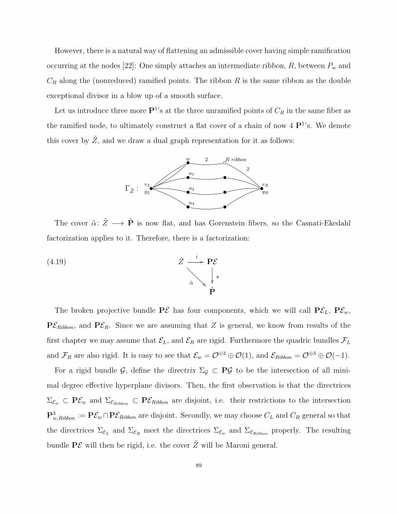
However, there is a natural way of flattening an admissible cover having simple ramification

occurring at the nodes [22]: One simply attaches an intermediate ribbon, R, between Pw and

CR along the (nonreduced) ramified points. The ribbon R is the same ribbon as the double

exceptional divisor in a blow up of a smooth surface.

Let us introduce three more P1’s at the three unramified points of CR in the same fiber as

the ramified node, to ultimately construct a flat cover of a chain of now 4 P1’s. We denote

this cover by Z, and we draw a dual graph representation for it as follows:

ΓZ : •vLgL •vRgR

•w

•a1

•a2

•a3

R ribbon

•

•

•

2

2

The cover α : Z −→ P is now flat, and has Gorenstein fibers, so the Casnati-Ekedahl

factorization applies to it. Therefore, there is a factorization:

(4.19) Zi//

α

PE

π

P

The broken projective bundle PE has four components, which we will call PEL, PEw,

PERibbon, and PER. Since we are assuming that Z is general, we know from results of the

first chapter we may assume that EL, and ER are rigid. Furthermore the quadric bundles FL

and FR are also rigid. It is easy to see that Ew = O⊕3 ⊕O(1), and ERibbon = O⊕3 ⊕O(−1).

For a rigid bundle G, define the directrix ΣG ⊂ PG to be the intersection of all mini-

mal degree effective hyperplane divisors. Then, the first observation is that the directrices

ΣEw ⊂ PEw and ΣERibbon ⊂ PERibbon are disjoint, i.e. their restrictions to the intersection

P3w,Ribbon := PEw∩PERibbon are disjoint. Secondly, we may choose CL and CR general so that

the directrices ΣEL and ΣER meet the directrices ΣEw and ΣERibbon properly. The resulting

bundle PE will then be rigid, i.e. the cover Z will be Maroni general.

89

The same type of analysis applies for F . First, it is easy to show that

Fw = O(1)⊕d−3 ⊕O⊕N

and that

FRibbon = O(−1)⊕d−3 ⊕O⊕N

The distinguished subvector bundle O(1)⊕d−3 → Fw parametrizes “quadrics splitting off

the plane spanned by the points a1, a2, and a3.” The sub vector bundle O⊕N → FRibbon

parametrizes “quadrics singular at the reduced point of the ribbon”.

When restricted to the intersection P3w,Ribbon := PEw ∩ PERibbon, these two distinguished

vector subspaces of F are complementary: The quadrics which split off the plane spanned

by a1, a2, and a3 and which contain the Spec k[ε]/(ε2) point of Pw ∩R will never be singular

at the reduced point of Pw ∩R, because the fibers of α are in general linear position.

The vector subbundles described in the previous paragraph give a description of the di-

rectrices of PFw and PFRibbon. Using this description, it is straightforward to show that one

can select CL and CR generically so that the directrices of PFL, PFw, PFRibbon, and PFR

meet properly.

The directrices of PFw and PFRibbon are disjoint, as we’ve seen. So we must show two

things. (1) There exists a genus gL degree 5 cover αL : CL −→ P1 and a triple of points

(a1, a2, a3) in a fiber α−1(x) such that the vector space of quadrics splitting off the plane

spanned by (a1, a2, a3) and containing α−1(x), properly intersects the distinguished vector

subspace of quadrics corresponding to the directrix subbundle of PFαL . (2) There exists

a genus gR degree 5 cover αR : CR −→ P1 and a ramified fiber α−1(y) = (2u1, u2, u3, u4)

(by this we mean u1 ∈ CR is a ramification point), such that the vector space of quadrics

singular at u1 and containing α−1(y) intersects the distinguished vector space of quadrics

corresponding to the directrix subbundle of PFαR .

90

For both of these, we simply refer the reader to the broken covers constructed in the

proof of Theorem 1.1 in chapter 1. By making these general choices, the cover Z will be

Casnati-Ekedahl general.

The relation resulting from our test family γ is

(4.20) c(E ′,Y) = 2c(E,Y) +11

10gR +

2

5g

(Note that we are relating a ramified divisor on the left hand side of the equation with an

unramified divisor on the right hand side of the equation.)

Now we use the same type of test family for the unramified, 2-vertex divisor E− which

has dual graph ΓE− :

•v−LgL+1

•v−R

gR−1

where we vary the left vertex v−L . As before, we obtain the relation

(4.21) c(E ′,Y) = 2c(E−,Y) +11

10(gL + 1) +

2

5g

Subtracting relations, we arrive at

(4.22) c(E,Y)− c(E−,Y) =11

20(gL + 1− gR)

91

Since we assume gR ≤ gL, we can conclude that c(E,Y) ≥ 0 once we know c(E0,Y) ≥ 0,

where ΓE0 is:

•vL

g−4•vR

0

However, one just uses a pencil of (1, 5) curves on P1 × P1 with 5 basepoints in a fiber, as

in chapter 3, section 3.1, to conclude c(E0,Y) ≥ 0.

Finally, notice that relation (4.20) also allows us to conclude that c(E ′,Y) ≥ 0 for any

simply-ramified 2-vertex divisor E ′.

4.5.2. Arbitrary 2-vertex divisors. For an arbitrary 2-vertex divisor, we use the same sort

of test family as we did in the previous section. We will only provide the starting point

of the construction, and will leave the details of the admissible reduction process to the

reader. Begin with a pencil p : Ct −→ P1t such that, for t = 0, the pentagonal curve C0 has a

prescribed ramification type. For example, if the divisor under consideration had dual graph

ΓE:

ΓE : •vL

gL•vRgR

3

2

then we would require our pencil P1t ⊂ PH0(P1,∧2F ⊗ E ⊗ detE∨) to have (2, 3) rami-

fication occurring somewhere, say s = 0, in the fiber C0. We pick P1t general among such

pencils. Again, we obtain a diagram

Ctα

##

P1t ×P1

s

π//

p

P1s

P1t

We pick the “section” curve D := α−1s = 0 ⊂ Ct so that, under the map p, D also

has ramification profile (2, 3) above t = 0. After a suitable base change and blowups, we

arrive at a family p with sections along which we may glue a constant family of curves on the92

left. (The procedure is essentially the same as the one described earlier.) The resulting test

family of admissible covers will entirely live inside an unramified 2-vertex divisor Eurn , and

will intersect a simply-ramified 2-vertex divisor Eram finitely many times. The relationship

between Eram and Eunr is exactly the same relationship as the one between E ′ and E−

above. The relation (4.20) shows that:

(4.23) c(Eram,Y) = 2c(Eunr,Y) +11

10gR +

2

5g

From this, and the relation coming from the test family γ constructed above, the positivity

of c(E,Y) will follow.

4.6. Some numerical observations. The main obstructions for determining slope bounds

for arbitrary d are: (1) The effective divisor class X is useless: the coefficient of D is not

negative, and (2) even if we had a useful candidate effect divisor class X, we would need

to exhibit sufficiently general test families to ensure that all coefficients of the divisor class

expression for X were negative.

Although the second obstruction seems completely beyond reach, we may still have a

chance of finding useful effective divisor classes X. Our first observation is this: For a

complete, one dimensional family T ⊂ Hd,g of covers, let

Cα//

ϕ

P

π

T

be the total diagram of the family. Let E and F denote the reduced direct image and bundle

of quadrics for the cover α : C −→ P . By Proposition 4.1, we see that the slope may be

written as:

s(T ) =δ · Tλ · T

=A(c2

1(E), c2(E), c2(F))

B(c21(E), c2(E), c2(F))

93

where A and B are linear expressions. The reader may check that after we set the Bogomolov

expressions Bog(E) and Bog(F) equal to zero, the the slope automatically becomes

sconj =(5d+ 6)g + d2 + 5d− 6

dg

Therefore, a complete family of curves T ⊂ Hd,g (passing through the interior) which com-

pletely avoids the Maroni and Casnati-Ekedahl divisors (when they exist) will automatically

attain the above conjectural slope bound.

On the other hand, for degrees d > 5, there is no effective combination of M and CE

which makes the coefficient of D zero. Therefore, we may have to venture beyond the world

of Maroni and Casnati-Ekedahl divisors. It is unclear how to proceed, however. For example,

in H6,g, we may want consider the higher syzygy divisor (when it exists) corresponding to

the Bogomolov expression for the bundle N3 occurring in the Casnati-Ekedahl resolution of

IC . After calculating, however, it unfortunately turns out that Bog(N2) = 2(Bog(F)).

However, all is not lost. One really should consider the Bogomolov expressions for all

vector bundles which arise from exact sequences among all tensor products of E and F . For

example, one may consider the Bogomolov expressions for the kernels of the “evaluation”

maps

SNE −→ α∗(ω⊗Nα ) −→ 0

Hopefully, one might be able to find a Bogomolov expression which, when written in terms

of λ, δ,D and higher boundary divisors, has negative contribution coming from δ,D, and the

rest of the boundary.

4.7. The congruence conditions on (g, d). Finally, we would like to comment on the

congruence conditions between g and d occurring in corollaries 4.8, 4.9, and 4.10. In [9], a

sharp slope bound for H3,g is obtained for odd g. This bound is 7 + 20/(3g + 1), and the

divisor X (which doesn’t exist) is replaced by the divisor of trigonal curves which are tangent

to the directrix of F1.94

4.8. A final fun example. We end by returning to the example in 1.4.1. The Maroni

divisor M ⊂ H3,4 parametrizes genus 4 curves which lie on a singular quadric in their

canonical embeddings. The branch divisor of a Maroni special cover α : C −→ P1 is a set

of 12 points on P1 whose defining equation has the form 4a3 + 27b2. In [9], we calculate

the exact class of M in PicQ H3,4. (This can also be done using partial pencil families.) By

pushing this class toM0,12, we recover a result originally due to Zariski [25]: The locus of 12

points on P1 which are zeros of a polynomial of the form 4a3 + 27b2 is 3762. This beautiful

example initiated our study of Maroni and Casnati-Ekedahl loci, so we find it a fitting way

to end.

References

[1] Dan Abramovich, Alessio Corti, and Angelo Vistoli. Twisted bundles and admissible covers. Comm.Algebra, 31(8):3547–3618, 2003.

[2] F. A. Bogomolov. Stable vector bundles on projective surfaces. Mat. Sb., 185(4):3–26, 1994.[3] G. Casnati and T. Ekedahl. Covers of algebraic varieties I. A general structure theorem, covers of degree

3, 4 and Enriques’ surfaces. J. Algebraic Geom., 5:439–460, 1996.[4] Gianfranco Casnati. Covers of algebraic varieties. II. Covers of degree 5 and construction of surfaces. J.

Algebraic Geom., 5(3):461–477, 1996.[5] Gianfranco Casnati. Covers of algebraic varieties. IV. A Bertini theorem for Scandinavian covers. Forum

Math., 13(1):21–36, 2001.[6] Marc Coppens. Existence of pencils with prescribed scrollar invariants of some general type. Osaka J.

Math., 36(4):1049–1057, 1999.[7] Maurizio Cornalba and Joe Harris. Divisor classes associated to families of stable varieties, with appli-

cations to the moduli space of curves. Ann. Sci. Ecole Norm. Sup. (4), 21(3):455–475, 1988.[8] Andrea Del Centina and Alessandro Gimigliano. Scrollar invariants and resolutions of certain d-gonal

curves. Ann. Univ. Ferrara Sez. VII (N.S.), 39:187–201 (1995), 1993.[9] A. Deopurkar and A. Patel. Sharp slope bounds for sweeping families of trigonal curves. ArXiv e-prints,

November 2012.[10] Anand Deopurkar. Modular compactifications of the space of marked trigonal curves. Preprint, 2012.[11] Steven Diaz and Joe Harris. Geometry of Severi varieties. II. Independence of divisor classes and ex-

amples. In Algebraic geometry (Sundance, UT, 1986), volume 1311 of Lecture Notes in Math., pages23–50. Springer, Berlin, 1988.

[12] Dan Edidin. Picard groups of Severi varieties. Comm. Algebra, 22(6):2073–2081, 1994.[13] John L. Harer. The cohomology of the moduli space of curves. In Theory of moduli (Montecatini Terme,

1985), volume 1337 of Lecture Notes in Math., pages 138–221. Springer, Berlin, 1988.[14] Joe Harris and David Mumford. On the Kodaira dimension of the moduli space of curves. Invent. Math.,

67(1):23–88, 1982.[15] Friedrich Knop, Hanspeter Kraft, and Thierry Vust. The Picard group of a G-variety. In Algebraische

Transformationsgruppen und Invariantentheorie, volume 13 of DMV Sem., pages 77–87. Birkhauser,Basel, 1989.

[16] S. Lefschetz. L’analysis situs et la geometrie algebrique. Gauthier-Villars, Paris, 1950.[17] Arturo Maroni. Le serie lineari speciali sulle curve trigonali. Ann. Mat. Pura Appl. (4), 25:343–354,

1946.

95

[18] Shinichi Mochizuki. The geometry of the compactification of the Hurwitz scheme. Publ. Res. Inst. Math.Sci., 31(3):355–441, 1995.

[19] David Mumford. Towards an enumerative geometry of the moduli space of curves. In Arithmetic andgeometry, Vol. II, volume 36 of Progr. Math., pages 271–328. Birkhauser Boston, Boston, MA, 1983.

[20] Akira Ohbuchi. On some numerical relations of d-gonal linear systems. J. Math. Tokushima Univ.,31:7–10, 1997.

[21] Sevin Recillas. Jacobians of curves with g14 ’s are the Prym’s of trigonal curves. Bol. Soc. Mat. Mexicana(2), 19(1):9–13, 1974.

[22] Zvezdelina E. Stankova-Frenkel. Moduli of trigonal curves. J. Algebraic Geom., 9(4):607–662, 2000.[23] Ilya Tyomkin. On Severi varieties on Hirzebruch surfaces. Int. Math. Res. Not. IMRN, (23), 2007.[24] Ravi Vakil. Twelve points on the projective line, branched covers, and rational elliptic fibrations. Math.

Ann., 320(1):33–54, 2001.[25] Oscar Zariski. On Hyperelliptic θ-Functions with Rational Characteristics. Amer. J. Math., 50(3):315–

344, 1928.

96