The Geometry of Maximum

Principles and a Bernstein Theorem

in Codimension 2

Renan Assimos and Jurgen Jost∗

Max Planck Institute for Mathematics in the Sciences

Leipzig, Germany

Moser’s Bernstein theorem [13] says that an entire minimal graph of codi-

mension 1 with bounded slope must be a hyperplane. An analogous result for

arbitrary codimension is not true, by an example of Lawson-Osserman. Here,

we show that Moser’s theorem nevertheless extends to codimension 2, i.e.,

a minimal p-submanifold in Rp+2, which is the graph of a smooth function

defined on the entire Rp with bounded slope, must be a p-plane. Our method

depends on convexity properties of Grassmannians which come into play as

the targets of the (harmonic) Gauss maps of our minimal submanifolds. In

fact, we develop a general method to construct subsets of complete Rieman-

nian manifolds that cannot contain images of non-constant harmonic maps

from compact manifolds. When applied to Grassmannians, for codimension

2, it yields an appropriate domain that cannot contain nontrivial images of

such harmonic maps. Our conclusion will then be reached by an application

of Allard’s theorem to handle the issue that the minimal submanifolds in

question are not compact.

Keywords: Bernstein theorem, minimal graph, harmonic map, Grassmannian, Gauss

map, maximum principle.

∗Correspondence: assimos@mis.mpg.de, jjost@mis.mpg.de

1

arX

iv:1

811.

0986

9v2

[m

ath.

DG

] 8

May

201

9

Contents

1 Introduction 2

2 Preliminaries 5

3 The Geometry of the Maximum Principle 7

3.1 Sampson’s Maximum Principle . . . . . . . . . . . . . . . . . . . . . . . 7

3.2 Barriers for the existence of harmonic maps . . . . . . . . . . . . . . . . 11

4 The Geometry of Grassmannian Manifolds 15

4.1 Basic definitions . . . . . . . . . . . . . . . . . . . . . . . . . . . . . . . . 15

4.2 Closed geodesics in G+p,n. . . . . . . . . . . . . . . . . . . . . . . . . . . . 18

4.3 Geodesically convex sets in G+p,n. . . . . . . . . . . . . . . . . . . . . . . . 20

5 Main Results 23

5.1 The slope of a graph . . . . . . . . . . . . . . . . . . . . . . . . . . . . . 23

5.2 Bernstein-type theorems for codimension 2 . . . . . . . . . . . . . . . . . 24

Bibliography 27

1 Introduction

One of the central results of the theory of minimal surfaces is Bernstein’s theorem, stating

that the only entire minimal graphs in Euclidean 3-space are planes. In other words, if

f(x, y) is a smooth function defined on all of R2 whose graph in R3, (x, y, f(x, y)), is a

minimal surface, then f is a linear function and its graph is a plane.

Profound methods in analysis and geometric measure theory were developed to generalize

Bernstein’s theorem to higher dimensions, culminating in the theorem of J. Simons

[16] stating that an entire minimal graph has to be planar for dimension d ≤ 7. This

dimension constraint is optimal, as Bombieri, de Giorgi, and Giusti [2] constructed

a counter-example to such an assertion in dimension 8 and higher. This reveals the

subtlety and difficulty of the problem. Under the additional assumption that the slope of

the graph is uniformly bounded, Moser [13] proved a Bernstein-type result in arbitrary

dimension.

All the preceding results consider minimal hypersurfaces, that is, minimal graphs in

Euclidean space of codimension 1. For higher codimension, the situation is more com-

plicated. On one hand, Lawson-Osserman [12] have given explicit counterexamples to

2

Bernstein-type results in higher codimension. Namely, the cone over a Hopf map is an

entire Lipschitz solution to the minimal surface system. Since the slope of the graph

of such a cone is bounded, even a Moser-type result for codimension higher than one

cannot hold.

On the other hand, there are also some positive results in higher codimension, although,

in view of the Lawson-Osserman examples, they necessarily require additional constraints.

We can describe the main development as a sequence of steps. Those results all depend on

the fact that, by a theorem of Ruh-Vilms [14], the Gauss map of a minimal submanifold

in Euclidean space is harmonic. This Gauss map takes its values in a Grassmann manifold

G+p,n (which is a sphere in the case of codimension n− p = 1). Therefore, the geometry

of Grassmann manifolds is the key to understanding the scope of Bernstein theorems

in higher codimension. Since the composition of a harmonic map (such as the Gauss

map) with a convex function is a subharmonic function, when such a convex function

is found the maximum principle can be applied to show that, when the domain of the

harmonic map is compact, the resulting subharmonic function is constant. And when

the convex function is nontrivial, for instance strictly convex, then the harmonic map

itself is constant, and the minimal graph is therefore linear. A key technical problem

emerges from the fact that in our application, the domain is Rp, which is not compact,

so that the maximum principle cannot be applied directly. We postpone the discussion

of this issue and return to the geometric steps.

1. Hildebrandt-Jost-Widman [7] identified the largest ball in the Grassmannian on

which the squared distance function from the center is convex. Thus, when the

Gauss image is contained in such a ball, that is, when the slopes of the tangent

planes of our minimal submanifold do not deviate too much from a given direction,

the minimal graph is linear, that is, a Bernstein result holds.

2. Why consider only distance balls? Jost-Xin [8] constructed regions in G+p,n which

are larger than convex metric balls but on which squared distance function is still

convex. After all, even though G+p,n is a symmetric space, the distance function

behaves differently in different directions. Thus, the Gauss region implying the

Bernstein results is larger.

3. Why consider only the squared distance function? Jost-Xin-Yang [10],[9] went

further by constructing larger regions in G+p,n that support strictly convex functions.

Thus, the Bernstein theorem was further extended. In particular in codimension 1,

that is, the classical case, even minimal hypersurfaces that might be more general

than graphs are shown to be linear. Still, it is not clear whether the Lawson-

3

Osserman example is sharp or whether there exist other examples that come closer

to the bounds obtained by [9] in higher codimension.

4. The level sets of convex functions are convex. The starting idea of the present paper

is that this is the key property: to have a family of convex hypersurfaces. But why

do we need convex functions? We show that a foliation by convex hypersurfaces

suffices, which does not need to come from a convex function. And this clarifies

the geometric nature of the maximum principle that was the cornerstone of the

reasoning just described. As far as we can tell, conceptually, this seems to be the

ultimate step in this line of research. Theorem 1.1, to be stated shortly, seems to

be the optimal result in codimension 2. It remains to explore our scheme in higher

codimension.

In fact, all those results apply more generally to graphs of parallel mean curvature, since

the Gauss map remains harmonic in such cases by the Ruh-Vilms theorem. It was proven

by Chern [4] that a hypersurface in Euclidean space that is an entire graph of constant

mean curvature necessarily is a minimal hypersurface. Thus, by Simons’ result, it is a

hyperplane for dimension d ≤ 7. See also Chen-Xin [3] for a generalization of Chern’s

result.

A maximum principle, however, only applies directly when the domain is compact, but

the domain of an entire minimal graph is Rp. Therefore, one needs to turn the qualitative

maximum principle into quantitative Harnack-type estimates, a technique also pioneered

by Moser [13]. In the proof of Hildebrandt-Jost-Widman [7], the analytical properties

of such convex functions were used to derive Holder estimates for harmonic maps with

values in Riemannian manifolds with an upper bound for the sectional curvature. By

a scaling argument, they could conclude a Liouville-type theorem for harmonic maps

under assumptions including the mentioned harmonic Gauss map. In the same setting,

Jost-Xin-Yang refined the tools developed in [7] and [8] to obtain a-priori estimates

for harmonic maps, improving higher codimension Bernstein results. Here, we use a

geometric maximum principle due to Sampson [15] (see also [5]), to develop a general

method for constructing subsets that do not admit images of non-constant harmonic maps

defined on compact manifolds. This method does not allow us to obtain Holder estimates,

but fortunately, we can replace them by the result of Allard [1], which is a seminal

results in geometric measure theory, to study the graph case and obtain Bernstein-type

results. For our purposes, Allard’s Theorem reduces the case of minimal submanifolds of

Euclidean space to that of minimal submanifolds of spheres. The corresponding Gauss

4

map for minimal submanifolds of spheres is still harmonic, so that the reasoning just

described still works.

More concretely, while Lawson-Osserman cones appear in codimension 3 or higher, we

prove a Moser-type result for codimension 2.

Theorem 1.1 (Moser’s Theorem in codim 2). Let zi = f i(x1, ..., xp), i = 1, 2, be smooth

functions defined everywhere in Rp. Suppose the graph M = (x, f(x)) is a submanifold

with parallel mean curvature in Rp+2. Suppose that there exists a number β0 < +∞ such

that

∆f (x) ≤ β0 for all x ∈ Rp, (1.1)

where

∆f (x) :={

det(δαβ +

∑i

f ixα(x)f ixβ(x))} 1

2 . (1.2)

Then f 1, f 2 are linear functions on Rp representing an affine p-plane in Rp+2.

The results of this paper constitute the main part of the first author’s PhD thesis. We

thank Lei Liu and Ruijun Wu for helpful discussions as well as Aleksander Klimek, Paolo

Perrone and Sharwin Rezagholi for helpful comments. We also thank Luciano Mari for

helping us to clarify some arguments on the previous version of this pre-print.

2 Preliminaries

Let (M, g) and (N, h) be Riemannian manifolds without boundaries. By Nash’s Theorem

we have an isometric embedding N ↪→ RL.

Definition 2.1. A map φ ∈ W 1,2(M,N) is called harmonic iff it is a critical point of

the energy functional

E(φ) :=1

2

∫M

‖dφ‖2dvolg, (2.1)

where ‖.‖2 = 〈., .〉 is the metric over the bundle T ∗M ⊗ φ−1TN induced by g and h.

Recall that the Sobolev space W 1,2(M,N) is defined as:

W 1,2(M,N) :={v : M −→ RL; ||v||2W 1,2(M) =

∫M

(|v|2 + ‖dv‖2) dvg < +∞ and (2.2)

v(x) ∈ N for almost every x ∈M}. (2.3)

5

The Euler-Lagrange equations for the energy functional are:

τ(φ) = 0, (2.4)

and τ is called the tension field of the map φ.

In local coordinates

e(φ) = ‖dφ‖2 = gij∂φβ

∂xi∂φγ

∂xjhβγ. (2.5)

τ(φ) =(∆gφ

α + gijΓαβγ∂φβ

∂xi∂φγ

∂xjhβγ) ∂

∂φα. (2.6)

where Γαβγ denote the Christoffel symbols of N.

Definition 2.2 (Gauss Map). Let Mp ↪→ Rn be a p-dimensional oriented submanifold

in Euclidean space. For any x ∈M , by parallel translation in Rn, the tangent space TxM

can be moved to the origin, obtaining a p-subspace of Rn, i.e., a point in the oriented

Grassmannian manifold G+p,n. This defines a map γ : M −→ G+

p,n called the Gauss map

of the embedding M ↪→ Rn.

Theorem 2.3 (Ruh-Vilms). Let M be a submanifold in Rn and let γ : M −→ G+p,n be

its Gauss map. Then γ is harmonic if and only if M has parallel mean curvature.

Harmonic maps have interesting geometric properties. By using Ruh-Vilms Theorem,

one can try to find subsets A ⊂ G+p,n for which there can be no non-constant harmonic

map φ defined on some compact manifold M with φ(M) ⊂ A. In that regard, it is often

useful to use the composition formula for φ : M −→ N , ψ : N −→ P where (P, i) is

another Riemannian manifold,

τ(ψ ◦ φ) = dψ ◦ τ(φ) + tr∇dψ(dφ, dφ). (2.7)

When φ is harmonic, i.e. τ(φ) = 0, the formula is particularly useful. In particular

if P = R, and ψ is a (strictly) convex function, then τ(ψ ◦ φ) ≥ 0 (> 0). That is,

ψ ◦ φ : M −→ R is a (strictly) subharmonic function on M. The maximum principle then

implies the following proposition:

Proposition 2.4. Let M be a compact manifold without boundary, φ : M −→ N a

harmonic map with φ(M) ⊂ V ⊂ N . Assume that there exists a strictly convex function

on V . Then φ is a constant map.

In our setting, the target N is the Grassmannian G+p,n. Then to obtain such a subset

A ⊂ G+p,n, one tries to find a strictly convex function f : A −→ R. This strategy was

used by Hildebrandt-Jost-Widman, Jost-Xin, Jost-Xin-Yang and others [7], [8], [9].

6

In this paper we want to modify this approach. Instead of using strong analytical

arguments to obtain a subset that admits a strictly convex function, we want to explore

the geometry of regions that can contain the image of a non-constant harmonic map.

To economize on notation, we state the following definition to be used throughout the

paper.

Definition 2.5 (Property (?)). We say that an open connected subset R ⊂ (N, h), where

(N, h) is a complete Riemannian manifold, has property (?) if there is no pair (M,φ),

where (M, g) is a compact manifold and φ : M −→ N is a non-constant harmonic map

with φ(M) ⊂ R.

3 The Geometry of the Maximum Principle

3.1 Sampson’s Maximum Principle

A beautiful result in the theory of harmonic maps is Sampson’s maximum principle

(SMP):

Theorem 3.1 (SMP). Let φ : (M, g) −→ (N, h) be a non-constant harmonic map, where

M is a compact Riemannian manifold, N is a complete Riemannian manifold, and

S ⊂ N is a hypersurface with definite second fundamental form at a point y = φ(x).

Then no neighborhood of x ∈M is mapped entirely to the concave side of S.

A proof can be found in [15] and [5].

Remark 3.2. Take a geodesic ball B(p, r) in a complete manifold N such that r is

smaller than the convexity radius of N at p. Then ∂B(p, r) is a hypersurface of N with

definite second fundamental form for every point q ∈ ∂B(p, r).

The main result of this work can be seen as a corollary of Sampson’s maximum principle.

Theorem 3.3. Let (N, h) be a complete Riemannian manifold and Γ : [a, b] −→ N a

smooth embedded curve. Consider a smooth function r : [a, b] −→ R+ and a region

R :=⋃t∈[a,b]

B(Γ(t), r(t)), (3.1)

where B(·, ·) is the geodesic ball and r(t) is smaller than the convexity radius of N for any

t. If, for each t0 ∈ (a, b), the set R\B(Γ(t0), r(t0)) is the union of two disjoint connected

sets, namely the connected component of Γ(a) and the one of Γ(b), then there exists

no compact manifold (M, g) and non-constant harmonic map φ : M −→ N such that

φ(M) ⊂ R. In other words, R has the property (?) of Definition 2.5.

7

φ harmonic

M cpt∂M = ∅

R :=⋃t∈[a,b] Bg(Γ(t), r)

r r ry1 = φ(x1)

φ(x) = y

x1

x

Γ(a)Γ(t)

Γ(b)

Figure 1: A region R as the union of convex balls

Before presenting the proof of this statement, we make two remarks on the geometry of

the region R

Remark 3.4. By hypothesis, for each time t0 ∈ [a, b], the set R\B(Γ(t0), r(t0)) is the

union of two disjoint connected components. This condition implicitly rules out a lot of

possibilities for both Γ and r. Namely, suppose we have a manifold with large convex

radius. We could define R as the union of balls over a geodesic of unit speed Γ of a very

small length ε with radius varying smoothly from ε/2 at t = 0, to 10ε at t = ε/2, and back

to ε/2 when t = ε. This region does not satisfies the necessary condition for our theorem.

On the other hand, suppose we have a curve Γ with the shape of a very steep ‘U ’. Our

condition implies that, in this case, the radius of the balls near the turning point of the

‘U’ must be very small, otherwise there will be some intersection between the connected

components of Γ(a) and Γ(b).

Lemma 3.5. Let R be a region defined as in Theorem 3.3 satifying the same hypothesis.

Let t0 ∈ (a, b) and consider the open set

Cb(t0) :=⋃

t∈(t0,b)

B(Γ(t), r(t))\(B(Γ(t0), r(t0))

)(3.2)

8

This is the connected component of Γ(b) in R\(B(Γ(t0), r(t0))). Then, for every point

y ∈ Cb(t0), there exists t1 > t0 such that y ∈ Cb(t1) and y ∈ ∂B(Γ(t1), r(t1)).

Proof. By definition of Cb(t0), whenever s′ > s, we have Cb(s′) ( Cb(s). Then for a

fixed y ∈ Cb(t0), we define the smooth function κy : [a, b] −→ R given by κy(s) :=

d(Γ(s), y)− r(s). Note that κy(t0) < 0.

Since

y ∈ Cb(t0) =⋃

t∈(t0,b)

B(Γ(t), r(t))\(B(Γ(t0), r(t0))

),

there exist t1 > t0 such that y ∈ B(Γ(t1, r(t1))

). This implies that κy(t1) > 0 and the

continuity of κ gives the existence of a point t1 ∈ R+ such that y ∈ Cb(t1).

Proof of Theorem 3.3: (See Figure 1) We argue by contradiction. Suppose that there

exists a compact manifold (M, g) and a non-constant harmonic map φ : M −→ N such

that φ(M) ⊂ R. Let φ(x) = y ∈ R be a point in φ(M). By definition of R and the fact

that φ is non-constant, there exists t0 ∈ [a, b] such that,

y ∈ ∂B(Γ(t0), r(t0)) ∩ Cb(t0),

where Cb(t) is defined by Equation (3.2). Therefore, by Sampson’s maximum principle,

for every open neighborhood Ux of x in M ,

φ(Ux) * B(Γ(t0), r(t0))

That is, there exists x1 ∈ Ux such that φ(x1) = y1 is mapped to the convex side of

B(Γ(t0, r(t0))). Moreover, as we assume that R\B(Γ(t0), r(t0)) is the union of two disjoint

connected sets, y1 ∈ Cb(t0). Therefore, by Lemma 3.5, there exists a t1 > t0 such that

y1 ∈ ∂B(Γ(t1), r(t1)) ∩ Cb(t1)

Again, by Sampson’s maximum principle, every open neighborhood Ux1 of x1 in M

satisfies

φ(Ux1) * B(Γ(t1), r(t1)),

that is, there exists x2 ∈ Ux1 such that φ(x2) =: y2 /∈ B(Γ(t1), r(t1)), y2 is in the convex

side of ∂B(Γ(t1), r(t1)) and in the same connected component as Γ(b). By induction, we

construct sequences {ti}i∈N and {yi}i∈N such that for every i ∈ N we have ti > ti+1 and

yi = φ(xi) ∈ φ(M) ∩ Cb(ti).Define t∗ = sup{t ∈ (a, b);φ(M) ∩ Cb(t) 6= ∅}. We claim that t∗ = b. Indeed, by

definition of t∗ and the fact that {ti} is a bounded monotone sequence, we have tj −→ t∗

9

p

A(p)

Figure 2: S2\(

12Eq)ε

and yj = φ(xj) ∈ Cb(tj) ⊂ Cb(tj−1) ⊂ ... ⊂ Cb(t0). Denoting by y∞ = limj→∞ yj,

we have y∞ = φ(x∞) ∈ Cb(t0) ∩ ... ∩ Cb(t∗) = Cb(t∗) and if t∗ < b we can apply

Sampson’s maximum principle to get a time t∗∗ such that t∗ < t∗∗ < b such that

φ(M) ∩ Cb(t∗∗) 6= ∅ which contradicts the fact that t∗ is the supremum of those times.

Hence y∞ ∈ ∂B(Γ(b), r(b)) ∩ ∂R and using once more Sampson’s maximum principle we

obtain a point y ∈ φ(M) \ R.

This result has very interesting applications.

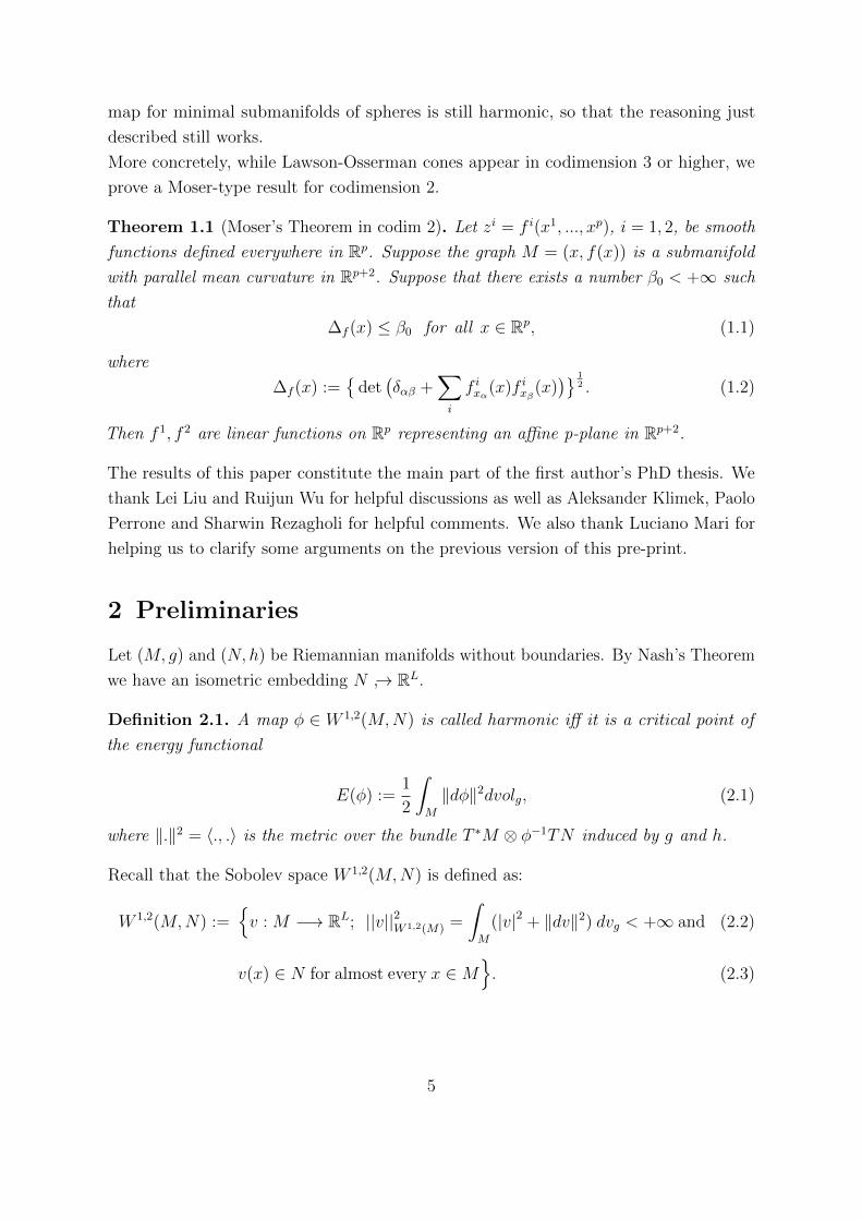
Example 3.6. Let (N, h) = (S2, g) ⊂ (R3, geuc) and let Γ : [0, 1] −→ S2 be the unit

speed geodesic such that Γ(0) = (−1, 0, 0), Γ(12) = (0, 0, 1) and Γ(1) = (1, 0, 0). For a

given ε > 0, let

R :=⋃t∈[0,1]

B(

Γ(t),π

2− ε

2

)(3.3)

and note that R contains the complement of an ε-neighborhood of the half equator

containing the points (0, 0,−1), (0,−1, 0) and (0, 1, 0), denoted by 12Eq. We will write R

as S2\(12Eq)ε. Theorem 3.3 implies that S2\(1

2Eq)ε has property (?).(See Figure 2)

Remark 3.7. The above argument also works for spheres Sn when we take out a closed

half equator, denoted by 12Sn−1. This result appears in [10], where is constructed a strictly

convex function on each compact subset properly contained in Sn\12Sn−1.

10

Remark 3.8. The main idea of the proof of Theorem 3.3 is that ∂R is a barrier to the

existence of non-constant harmonic maps. With the help of the SMP and the definition

of R as a union of convex balls, we push the image of the harmonic map to this barrier.

One can make the theorem more general by simply changing ∂R ∩ ∂B(Γ(b), r(b)) to some

more flexible barrier. For example, with a similar family of balls that we defined in

Example 3.6, one would prove that there are no non-constant harmonic maps whose

image is contained in an open subset of S2\γ where γ is a connected curve connecting

the antipodal points (0, 1, 0), (0,−1, 0) ∈ S2.

Note that the classical method used to prove non-existence of such non-constant harmonic

maps, i.e., the method of looking for a strictly convex function f : R −→ R (in the

geodesic sense), is not very flexible. Once one changes the boundary of R slightly, one

can no longer guarantee that there exists a strictly convex function f : R −→ R.

3.2 Barriers for the existence of harmonic maps

Our proof of Theorem 3.3 gave the barrier for the existence of harmonic maps as the

boundary of the union of a family of balls whose centers are given by a smooth embedded

curve.

By studying barriers to the existence of harmonic maps abstractly, we find that the result

does not rely on the existence of such a family of balls along a curve.

The region R defined in Example 3.6 contains no closed geodesics, and since geodesics

are harmonic maps, it is necessary to avoid them for the non-existence of non-constant

harmonic maps. Therefore the first condition we are looking for is one that avoids such

curves.

Condition 1. For every p ∈ R and every v ∈ T 1pN , the geodesic Γ such that Γ(0) = p

and Γ′(0) = v satisfies, for some tv ∈ [0, K], Γ(tv) ∈ ∂R. Where K is independent of p

and v.

Condition 1 is a qualitative way of imposing the non-existence of closed geodesics in

our region. But imposing the non-existence of closed geodesics in a given region is not

enough to avoid existence of harmonic maps, therefore we need an extra condition to be

stated later. But first, let us introduce some notation.

Notation 3.9. For p ∈ N and v ∈ TpN , we denote by γp,v : R −→ N the geodesic that

satisfies γp,v(0) = p and γ′p,v(0) = v.

As an example, suppose we have a point in the image of some geodesic, namely Γp,v(t0).

Take a tangent vector η ∈ TΓp,v(t0)N such that η 6= Γ′p,v(t0). If we consider another geodesic

passing through Γp,v(t0) in the direction η at t = 0 , we write γΓp,v(t0),η(·) : R −→ N .

11

Notation 3.10. For p ∈ N , ν ∈ ∂Bg(p, r) with r � 1, let tmax(p, ν) ∈ R+ be the first

time at which Γp,ν(t) ∈ ∂R.

We impose the following condition on the region R.

Condition 2. For every p ∈ R and every ν ∈ T 1pN , if t < tmax(p, ν), then the set of

directions{η ∈ T 1

Γp,ν(t)N | d(p, γRΓp,ν(t),η(ε)) < d(p,Γp,ν(t))}

is properly contained in T 1Γp,ν(t)

and connected. Here γR is a geodesic in R with ε ∈ R+ sufficiently small (that is, a curve

that minimizes the length in R).

In general, Condition 2 is difficult to check unless N is a symmetric space and one

understands very well the geometry of the region R.

Theorem 3.11. Let (N,h) be a complete Riemannian manifold and suppose that for

a region R ⊂ N , R \ ∂R is open and connected. In addition, suppose R satisfies the

Conditions 1 and 2 above. Then R has property (?) of Definition 2.5.

Proof. We argue by contradiction. Suppose that there exists a compact manifold (M, g)

and a non-constant harmonic map φ : M −→ N such that φ(M) ⊂ R. Therefore, there

exist points p = φ(x), q ∈ R such that d(q, p) � 1 and a geodesic Γ with Γ(0) = p,

Γ′(0) = vp,q, and Γ(tp) = q. By Condition 1 there exists tvp,q ∈ R+ such that Γ intersects

∂R. Define

Q0 := ∪t∈R+B(Γ(t), δ), with δ > δ0 > 0,

and note that it satisfies the conditions of Theorem 3.3.

Therefore, when walking along Γ with the ball B(Γ(t), δ), there exists q1 /∈ Q0 such that

q1 = φ(y1), y1 ∈M , and Condition 2 tells us that

dR(q1, p) > dR(q, p).

Let γR1 be a curve in R, connecting p and q1, of minimal length. Note that it may not be

a geodesic in N itself. By Condition 2, there exists η1 ∈ T 1q1N such that Γq1,η1 increases

the distance to p, that is,

dR(Γq1,η1(t), p) > dR(q1, p)

for sufficiently small t (as before, Γq1,η1 hits the boundary at some point tq1 by Condition 1).

Now let

Q1 := ∪t∈R+B(Γq1,η1(t), δ1), δ1 > δ0.

By Theorem 3.3, there exist q2 ∈ Q1 such that q2 = φ(y2) and

dR(q2, p) > dR(q1, p) > dR(q, p).

12

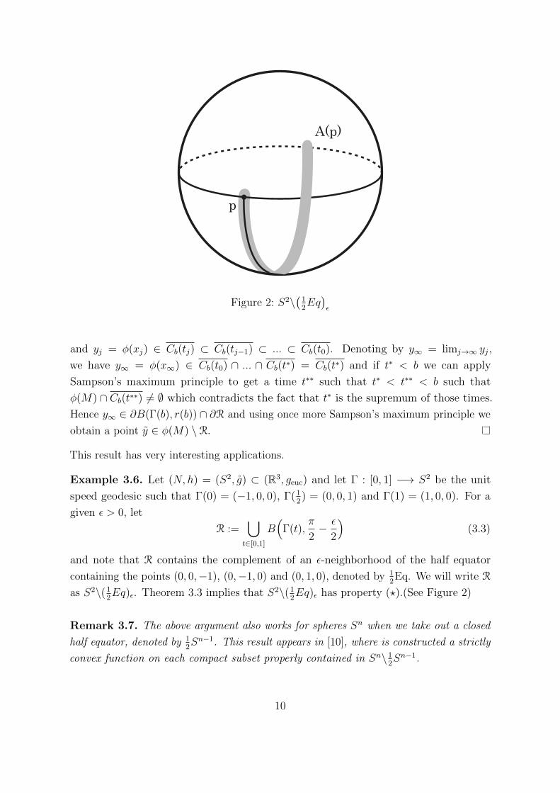
φ

harmonic

M compact

∂M = ∅

Figure 3: Example of barriers for the existence of harmonic maps in immersed surfaces

in R3 of genus one, two and three.

Inductively, we build a sequence of points q1, q2, q3, ... such that qi = φ(yi) with yi ∈Mfor all i ∈ N and

dR(qi, p) = dR(qi, φ(x)) > dR(qi−1, φ(x)).

Arguing like in the proof of 3.3, we obtain that y∞ = φ(x∞) ∈ φ(M) ∩ ∂R and therefore

by Sampson’s maximum principle there exists a point y ∈ φ(M) \ R.

Example 3.12. One can use the above theorem to find regions in symmetric spaces for

which property (?) holds. If one has some information about the geometry of such a

space, Conditions 1 and 2 may be easy to check. For instance, let p ≥ 1 and (Σp, g) be a

compact surface of genus p with a hyperbolic metric of constant curvature. Let γ1, ..., γ2p

be smooth curves that generate H1(Σp,R), the first homology group of Σp. For a given

ε > 0, define

R := Σp\(γ1 ∪ ... ∪ γ2p)ε (3.4)

We see that R satisfies Conditions 1 and 2, therefore it has property (?). See Figure 3.

An alternative proof of this statement could be given simply by noting that a harmonic

map defined on a compact manifold and taking values in a polygon with 4p-sides in the

Poincare hyperbolic space such that its image is contained in the interior of this polygon

must be constant. The example above is just to illustrate the relations between such

property of harmonic maps and maximum principles.

To use the previous results to obtain Bernstein-type theorems we have to overcome the

compactness of M . We will be able to do so for the graph case and the harmonic map

13

that we are taking into consideration is the Gauss map. We state that precisely in the

following theorem.

Theorem 3.13 (Property (?) for graphs). Let M = graph(f) be a minimal submanifold,

where f : Rp −→ Rn−p is a smooth map with bounded slope, and let γ : M −→ G+p,n be its

normal Gauss map. Suppose γ(M) ⊂ R, where R is a region in G+p,n that has property

(?). Then the harmonic Gauss map is constant and M is a plane.

Proof. Let C(M,∞) be the tangent cone of M at ∞ defined as follows. Considering the

family ft = 1tf(t.x) indexed on R+ and the set {Mt = graph(ft) : t ∈ R+}, it is known

that ft satisfies the minimal surface equations and hence {Mt = graph(ft) : t ∈ R+} de-

fines a family of minimal submanifolds in Rn. Using the same argument as Fischer-Colbrie

in [6], we show that {ft : t ∈ R+} is an equicontinuous family on any compact subset

of Rp, thus Arzela-Ascoli implies that there exists a subsequence fti : i ∈ N such that

limi→+∞ = +∞ and limi→+∞ fti = h, where h is a Lipschitz function and a weak solution

to the minimal surface equation, and its graph C(M,∞) := {(x, h(x)) : x ∈ Rn} is a

cone, which is called the tangent cone of M at ∞.

If the cone C(M,∞) is regular except in the origin, then the intersection of C(M,∞) and

the unit sphere Sn−1 gives a (p−1)-dimensional embedded compact minimal submanifold

of Sn−1, which is denoted by M ′ ([16]). Since the normal Gauss map is a cone-like map,

the image of the normal Gauss map of M ′ is still contained in the region R. M ′ is

compact and minimal in Sn−1, hence M ′ has parallel mean curvature and is compact in

Rn. Thus the fact that γ(M ′) ⊂ R and the region R has property (?) implies that M ′ is

a totally geodesic subsphere of Sn−1. Then Allard’s regularity in [1] implies that f is an

affine map and M a p-plane.

If the cone C(M,∞) has a singularity at a point p0 6= 0, we consider a blow-up at p0 and

obtain a tangent cone of the tangent cone C(M,∞) at p0, which is a product of the form

C ×R, and C is a minimal cone of dimension (p− 1) in Rn−1, which is also a graph and

the slope is bounded everywhere. If C is smooth except at the origin, we can proceed as

above to prove that C is an affine (p− 1)-plane, which gives a contradiction. Otherwise,

we iterate the above argument until we have obtained a minimal cone of dimension 1,

which cannot be singular once more giving a contradiction. Therefore 0 ∈ Rn is the only

possible singularity for C(M,∞) and hence M is an affine p-plane.

In section 4, we will use this to study regions on the Grassmannian manifold where the

14

harmonic Gauss map from a minimal submanifold may, or may not, be constant.

4 The Geometry of Grassmannian Manifolds

We first need to recall some facts about Grassmannians as stated in Kozlov [11] and

Jost-Xin [8].

4.1 Basic definitions

Let V n be an n-dimensional vector space over R with inner product 〈., .〉. One defines a

2n-dimensional algebra with respect to the exterior product ∧ by

Λ(V ) = ⊕∞i=0Λi(V ) (4.1)

such that Λ0(V ) = R, Λ1(V ) = V and Λi>n(V ) = 0. Λ(V ) is called the Grassmann

algebra and the elements of Λp(V ) are called p-vectors. When V = Rn, we denote Λp(Rn)

simply by Λp.

Let {ei}ni=1 be a basis for V and λ = (i1, ..., ip) ∈ Λ(n, p) = {(i1, ...ip); 1 ≤ i1 < ... < ip ≤n}. We denote by eλ the p-vector

eλ := ei1 ∧ ... ∧ eip (4.2)

{eλ}λ∈Λ(n,p) is a basis for the(np

)-dimensional vector space Λp(V ) ⊂ Λ(V ). For any

w ∈ Λp(V ),

w =∑

λ∈Λ(n,p)

wλeλ (4.3)

Definition 4.1 (Simple vector). A p-vector w ∈ Λp(V ) is called simple if it can be

represented as the exterior product of p elements of V, that is, w = af1 ∧ ... ∧ fp, with

a ∈ R and fi ∈ V for every i ∈ {1, ..., p}.

Definition 4.2 (Scalar product of p-vectors). The scalar product of two p-vectors w and

w is the number

〈w, w〉 :=∑

λ∈Λ(n,p)

wλwλ (4.4)

One can prove that this product has the properties of a scalar product and does not

depend on the choice of the orthonormal basis. We also have that |w| = 〈w,w〉12 .

15

Definition 4.3 (Inner multiplication of p-vectors). An operation of inner multiplication

is a bilinear map

x: Λp(V )× Λq(V ) −→ Λp−q(V ), p ≥ q ≥ 0 (4.5)

(ω, ξ) 7→ wxξ (4.6)

that for any ω ∈ Λp(V ), ξ ∈ Λq(V ), and ϕ ∈ Λp−q(V ) satisfies

〈ωxξ, ϕ〉 = 〈ω, ξ ∧ ϕ〉 (4.7)

Definition 4.4 (The rank space). The rank space of a p-vector w ∈ Λp(V ) (p ≥ 1) is

defined as

Vw = wxΛp−1(V ) = {e ∈ V ; e = wxv, v ∈ Λp−1(V )} ⊂ V (4.8)

That is, Vw ⊂ V is the minimum subspace W ⊂ V such that w ∈ Λp(W ).

Remark 4.5. A nonzero w ∈ Λp(V ) is simple if, and only if, dimVw = p.

Therefore there is a one-to-one correspondence between the set of oriented p-planes and

the set of unit simple p-vectors. This will be important when we define the so called

Plucker embedding of the Grassmannian manifold.

Definition 4.6 (Grasmannian manifold G+p,n). Let Rn be the n-dimensional Euclidean

space. The set of all oriented p-subspaces (called p-planes) constitutes the Grassmannian

manifold G+p,n, which is the irreducible symmetric space SO(n)/(SO(p)× SO(q)), where

q = n− p.

For each p-plane V0 ∈ G+p,n, consider the open neighborhood U(V0) of all oriented p-planes

whose orthogonal projection into V0 is one-to-one. That is, if {ei}pi=1 is an orthonormal

basis of V0, and {nα}qα=1 is an orthonormal basis of V ⊥0 , one can write, for V ∈ U(V0),

ei(V ) = ei +Ni (4.9)

where Ni ∈ V ⊥0 and ei(V ) ∈ V is such that ei = PrV0(ei(V )).

Decomposing the vector Ni using the basis {nα} gives us a matrix a = (aαi ) ∈ Rp.q defined

by

Ni = aαi nα (4.10)

that can be regarded as local coordinates of the p-plane V in U(V0).

16

Using the one-to-one correspondence between unit simple vectors and oriented p-planes

V ∈ G+p,n we define the Plucker embedding as

ψ : G+p,n −→ Λp

ψ(V ) :=ψ(V )

|ψ(V )|,

(4.11)

where

ψ(V ) := (e1 +N1) ∧ ... ∧ (ep +Np), . (4.12)

Via the Plucker embedding, G+p,n can be viewed as a submanifold of the Euclidean space

R(np). The restriction of the Euclidean inner product denoted by ω : G+p,n ×G+

p,n −→ R,

is

ω(P,Q) =〈ψ(P ), ψ(Q)〉

〈ψ(P ), ψ(P )〉 12 〈ψ(Q), ψ(Q)〉 12. (4.13)

If {e1, ..., ep} is an oriented orthonormal basis of P and {f1, ..., fp} is an oriented or-

thonormal basis of Q, then

w(P,Q) = 〈e1 ∧ ... ∧ ep, f1 ∧ ... ∧ fp〉 = detW, (4.14)

where W = (〈ei, fj〉).

Remark 4.7. Note that ψ(G+p,n) = Kp ∩ S(np)−1 ⊂ R(np) ∼= Λp.

Remark 4.8. Let w ∈ ψ(G+p,n) and {ei}pi=1, {nα}qα=1 be an orthonormal basis for Vw and

V ⊥w , respectively. The system of vectors {ηiα}p , qi=1,α=1 where

ηiα = e1 ∧ ... ∧ ei−1 ∧ nα ∧ ei+1 ∧ ... ∧ ep, (4.15)

for i ∈ {1, ..., p} and α ∈ {1, ..., q} is an orthonormal basis of the tangent space

Tw(ψ(G+p,n)).

We will write G+p,n instead of ψ(G+

p,n) for the image of the Grassmannian manifold under

the Plucker embedding.

Let (w,X) ∈ TG+p,n be an element of the tangent bundle and {ηiα}α=1,...,q

i=1,...,p a basis for

TwG+p,n like above. There exist mi ∈ V ⊥w such that

X = m1 ∧ e2 ∧ ... ∧ ep + ...+ e1 ∧ ... ∧ ep−1 ∧mp. (4.16)

These mi are not necessarily pairwise orthogonal.

17

Theorem 4.9 (Kozlov). Let w ∈ G+p,n and X ∈ TwG

+p,n, X 6= 0. Then there exists

an orthonormal basis {ei}pi=1 in Vw and a system {mi}ri=1, with 1 ≤ r ≤ min{p, q}, of

non-zero pairwise orthogonal vectors in V ⊥w , such that

w =e1 ∧ ... ∧ ep, (4.17)

X =(m1 ∧ e2 ∧ ... ∧ er + ...+ e1 ∧ ... ∧ er−1 ∧mr) ∧ (er+1 ∧ ... ∧ ep). (4.18)

Notation 4.10. Based on Equation (4.17) and Equation (4.18) above, we write

λi := |mi|, ni :=mi

λi, (4.19)

ei(s) := ei cos(s) + ni sin(s), ni(s) := −ei sin(s) + ni cos(s), (4.20)

X0 := er+1 ∧ ... ∧ ep. (4.21)

Note that e′i(s) = ni(s) and n′i = −ei(s),

4.2 Closed geodesics in G+p,n.

Consider the curve

w(t) := e1(λ1t) ∧ ... ∧ er(λrt) ∧X0. (4.22)

Theorem 4.11. The curve w(t) is a normal geodesic in the manifold G+p,n and

expwX = w(1) (4.23)

Proof(Sketch). For each t ∈ R, {ei(λit), ni(λit)}ri=1 are pairwise orthogonal vectors and

e′i(λit) =λini(λ

it), n′i(λit) = −λiei(λit), (4.24)

X(t) :=w′(t) =r∑i=1

λini(λit) ∧ (w(t)xei(λ

it)), (4.25)

w(0) = w, w′(0) = X, |X(t)| =

[r∑i=1

(λi)2

] 12

. (4.26)

Therefore w(t) is parametrized proportionally to the arc-length. Moreover, taking an

additional derivative, we have

w′′(t) = −|X|2w(t) + ξ(t), (4.27)

where ξ(t) is a term like Equation (4.25) with ni replacing the ei and therefore orthogonal

to the tangent plane Tw(t)G+p,n.

18

We will denote the above geodesic by

wX(t) := e1(λ1t) ∧ ... ∧ er(λrt) ∧X0, (4.28)

where X = (λ1n1 ∧ e2 ∧ ... ∧ er + λ2e1 ∧ n2 ∧ ... ∧ er + ...+ λre1 ∧ ... ∧ er−1 ∧ er) ∧X0.

Thus a geodesic in G+p,n between two p-planes is simply obtained by rotating one into the

other in the Euclidean space, by rotating corresponding basis vectors. As an example

the 2-plane spanned by e1, e2 in R4: one tangent direction in G+2,4 would be to move

e1 into e3 and keep e2 fixed, and the other tangent direction would be to move e2 into

e4 and keep e1 fixed. In other words, we are taking X, Y ∈ TwG+2,4, for some w ∈ G+

2,4,

where X = e3 ∧ e2 and Y = e1 ∧ e4 and the respective geodesics are given by equation

(4.28). We can also consider Z ∈ TwG+2,4 where Z := ( 1√

2e3 ∧ e2 + 1√

2e1 ∧ e4) and the

respective geodesic wZ(t) given by equation (4.28) is obtained when we simultaneously

rotate e1 into e3 and e2 into e4. This is a geometric picture that helps to understand

our subsequent constructions. Later we compute the length of these different types of

geodesics in a general Grassmannian.

Theorem 4.12. For G+p,n, we have

diam(G+p,n) = max

{π,√r0π/2

}, (4.29)

where r0 = min{p, q}. More explicitly,

r0 < 4⇒ diam(G+p,n) = π, (4.30)

r0 ≥ 4⇒ diam(G+p,n) =

√r0π

2. (4.31)

For the next examples, we have to understand the closed geodesics in G+p,n.

Theorem 4.13. For geodesics in G+p,n with parametrization (4.28), we have that

wX(t1) = wX(t2) ⇐⇒ ∃k ∈ Zr; λi(t2 − t1) = πki, andr∑i=1

ki ≡ 0 mod 2. (4.32)

Remark 4.14. In particular, every geodesic loop in G+p,n is a closed geodesic.

This assertion can be used to compute lengths of closed geodesics in G+p,n, because

L(wX) = |X| =

[r∑i=1

(λi)2

] 12

. (4.33)

19

4.3 Geodesically convex sets in G+p,n.

As we have mentioned in the previous section, we are interested in the convex sets in a

Grassmannian manifold.

Let w ∈ G+p,n and X ∈ TwG

+p,n a unit tangent vector. We know that there exists an

orthonormal basis {ei, nα}α=1,...,qi=1,...,p of Rn and a number r ≤ min(p, q) such that w =

span{ei}, n = p+ q and

X =(λ1n1 ∧ e2 ∧ ... ∧ er + ...+ λre1 ∧ ... ∧ er−1 ∧ nr

)∧X0, (4.34)

and |X| =(∑r

α=1|λα|2) 1

2 = 1.

Definition 4.15. Let X ∈ TwG+p,n be given by Equation (4.34). Define

tX :=π

2(|λα′ |+ |λβ′ |), (4.35)

where |λα′ | := max{λα} and |λβ′ | := max{λα; λα 6= λα′}.

Definition 4.16. Let w ∈ G+p,n and X ∈ TwG

+p,n a unit tangent vector like in Equa-

tion (4.34). Define

BG(w) := {wX(t) ∈ G+p,n; 0 ≤ t ≤ tX}.

Theorem 4.17 (Jost-Xin). The set BG(w) is a (geodesically) convex set and contains

the largest geodesic ball centered at w.

Now we are going to present some explicit examples of geodesics in G+p,n and compute at

which time they intersect the region we have defined above. Those examples clarify how

geodesics behave in Grassmannian manifolds, and thereby the geometry of BG(w).

Example 4.18. Let w = e1 ∧ ... ∧ ep ∈ G+p,n and denote X1 = n1 ∧ e2 ∧ ... ∧ ep. From

the notation above λ1 = 1 and λi = 0 for every i 6= 1. Moreover |X1| = 1 and tX1 = π2.

Thus the length of this closed geodesic is 2π. Moreover, denoting by |L(wX(t))| the

length of the segment connecting wX(0) and wX(t), we have |L(wX1(tX1))| = π2. Clearly,

wX1(π) = −w and, as G+p,n is a symmetric space, wX1(−ε) = w−X1(ε), so wX1 : R −→ G+

p,n

is a geodesic such that γ|[−π2 ,π2 ] ⊂ BG(w).

It is known that G+p,n is a submanifold of S(np)−1 ⊂ R(np) with the induced metric of the

sphere. So in the direction X1, BG(w) contains half of a great circle connecting two

antipodal points.

20

Example 4.19. Consider w = e1∧...∧ep ∈ G+p,n and X2 = 1√

2(n1∧e2+e1∧n2)∧e3∧...∧ep.

Therefore X2 ∈ TwG+p,n with |X2| = 1. Moreover in the definition of BG(w):

tX2 =π

2( 1√2

+ 1√2)

=

√2π

4=

√2

2

π

2<π

2. (4.36)

Thus, to make tX as small as possible, we need an equidistribution of the eigenvalues λα of

X satisfying∑

α|λα| = 1 and we maximize λmax+λmax′ . In this case, wX2

(√2π4

)∈ ∂BG(w)

is the point in the boundary closest to w. Also, by Theorem 4.13

wX2(t) = wX2(0) = w ⇐⇒ ∃k1, k2 ∈ Z2; λi(t− 0) = π.ki and k1 + k2 = 0 (mod 2)

(4.37)

but

λ1 = λ2 = 1/√

2 , therefore t =√

2k1π =√

2k2π. (4.38)

Then k1 = k2 = 1 solves the equation and tells us that wX2(√

2π) = w, and, as wX2 is

parametrized by arc length,

L(wX2) =√

2π = 4tX2 . (4.39)

By [11], this is the smallest non-trivial closed geodesic in G+p,n, r0 > 1.

It will be crucial below that the equation for the geodesic wX2 is

wX2(t) =

(e1 cos

(t√2

)+ n1 sin

(t√2

))∧(e2 cos

(t√2

)+ n2 sin

(t√2

))∧(e3 ∧ ... ∧ ep),

(4.40)

so we compute, for any t ∈ R,

〈wX2(t), w〉 =⟨(e1 cos(t/

√2) + n1 sin(t/

√2))

∧(e2 cos(t/

√2) + n2 sin(t/

√2)), (e1 ∧ e2)

⟩·⟨

(e3 ∧ ... ∧ ep), (e3 ∧ ... ∧ ep)⟩

=⟨e1 cos

(t/√

2), e1

⟩·⟨e2 cos

(t/√

2), e2

⟩= cos2

(t√2

)≥ 0

(4.41)

Therefore, using the fact that G+p,n ⊂ S(np)−1 and denoting the antipodal point in S(np)

by −w, the geodesic wX2 never leaves the hemisphere of S(np) that has w as a pole. In

particular wX2(t ∈ R+) does not intersect BG(−w).

21

Example 4.20. Consider w = e1 ∧ ...∧ ep ∈ G+p,n and Xr0 = 1√

r0(n1 ∧ e2 ∧ ...∧ er0 + ...+

e1 ∧ ... ∧ er0−1 ∧ nrr0 ) ∧ er0+1 ∧ ... ∧ ep, so that Xr0 ∈ TwG+p,n with |Xr0 | = 1. Therefore

tXr0 =π

2( 1√r0

+ 1√r0

)=

√r0π

4, (4.42)

and the geodesic wXr0 lies inside BG(w). As before, G+p,n is a symmetric space, thus the

curve wXr0 : (−√r0π

4,√r0π

4) −→ G+

p,n is a geodesic with w−Xr0 (−√r0π

4) = wXr0 (

√r0π

4) and

wXr0 (t) = wXr0 (0) = w ⇐⇒ ∃k1, ..., kr0 ∈ Zr0 ; λi(t− 0) = π.ki

and

r0∑r0=1

ki = 0 (mod 2)(4.43)

thus λi = 1/√r0 and t =

√r0k

iπ for every i ∈ {1, ...r0}.Consequently, if r0 is an even number, then ki = 1 solve the equation and tell us that

wXr0 (√r0π) = w, and, as wXr0 is parametrized by arc length,

∣∣L(wXr0 )∣∣ =√r0π (= 4tr0);

if r0 is an odd number, then ki = 2 solve the equation and tell us that wXr0 (√r0π) = w,

and, as wXr0 is parametrized by arc length,∣∣L(wXr0 )

∣∣ = 2√r0π (= 8tr0).

The equation for the geodesic wXr0 is

wXr0 (t) =

(e1 cos

(t√r0

)+ n1 sin

(t√r0

))∧(e2 cos

(t√r0

)+ n2 sin

(t√r0

))∧

... ∧(er0 cos

(t√r0

)+ nr0 sin

(t√r0

))∧ (er0+1 ∧ ... ∧ ep)

(4.44)

so we compute for any t ∈ R+

〈wXr0 (t), w〉 = 〈(e1 cos(t/

√r0) + n1 sin(t/

√r0)), e1〉·

〈(e2 cos(t/

√r0) + n2 sin(t/

√r0)), e2〉 · · ·

〈(ei cos(t/

√r0) + ni sin(t/

√r0)), ei〉 · · ·

〈(er0 cos(t/

√r0) + nr0 sin(t/

√r0)), 〉·

〈(er0+1 ∧ ... ∧ ep), (er0+1 ∧ ... ∧ ep)〉

= 〈e1 cos(t/√r0), e1〉 · · · 〈er0 cos(t/

√r0), er0〉 = cosr0(t/

√r0)

(4.45)

Note that if r0 is odd, then wXr0 (0) and wXr0 (√r0π) are antipodal points in S(np)−1. Also,

〈wXr0 (t), w〉 ≥ 0 and wX0 does not intersect BG(−w) if and only if r0 is even.

22

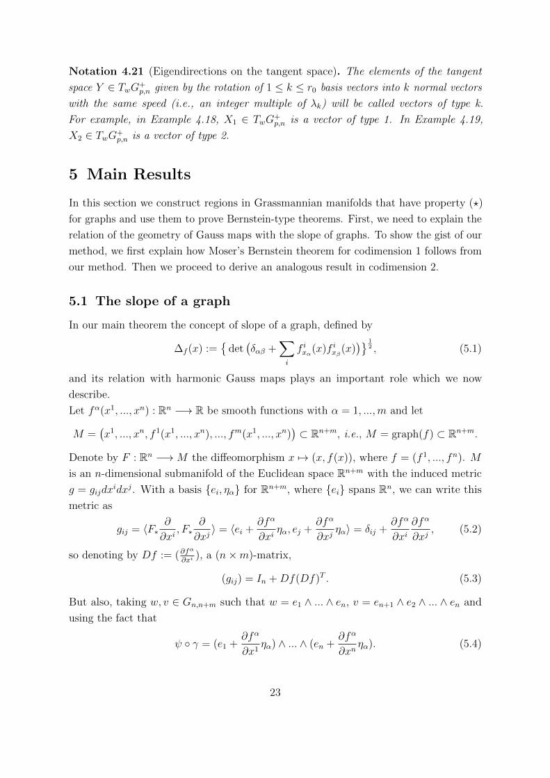
Notation 4.21 (Eigendirections on the tangent space). The elements of the tangent

space Y ∈ TwG+p,n given by the rotation of 1 ≤ k ≤ r0 basis vectors into k normal vectors

with the same speed (i.e., an integer multiple of λk) will be called vectors of type k.

For example, in Example 4.18, X1 ∈ TwG+p,n is a vector of type 1. In Example 4.19,

X2 ∈ TwG+p,n is a vector of type 2.

5 Main Results

In this section we construct regions in Grassmannian manifolds that have property (?)

for graphs and use them to prove Bernstein-type theorems. First, we need to explain the

relation of the geometry of Gauss maps with the slope of graphs. To show the gist of our

method, we first explain how Moser’s Bernstein theorem for codimension 1 follows from

our method. Then we proceed to derive an analogous result in codimension 2.

5.1 The slope of a graph

In our main theorem the concept of slope of a graph, defined by

∆f (x) :={

det(δαβ +

∑i

f ixα(x)f ixβ(x))} 1

2 , (5.1)

and its relation with harmonic Gauss maps plays an important role which we now

describe.

Let fα(x1, ..., xn) : Rn −→ R be smooth functions with α = 1, ...,m and let

M =(x1, ..., xn, f 1(x1, ..., xn), ..., fm(x1, ..., xn)

)⊂ Rn+m, i.e., M = graph(f) ⊂ Rn+m.

Denote by F : Rn −→M the diffeomorphism x 7→ (x, f(x)), where f = (f 1, ..., fn). M

is an n-dimensional submanifold of the Euclidean space Rn+m with the induced metric

g = gijdxidxj. With a basis {ei, ηα} for Rn+m, where {ei} spans Rn, we can write this

metric as

gij = 〈F∗∂

∂xi, F∗

∂

∂xj〉 = 〈ei +

∂fα

∂xiηα, ej +

∂fα

∂xjηα〉 = δij +

∂fα

∂xi∂fα

∂xj, (5.2)

so denoting by Df := (∂fα

∂xi), a (n×m)-matrix,

(gij) = In +Df(Df)T . (5.3)

But also, taking w, v ∈ Gn,n+m such that w = e1 ∧ ... ∧ en, v = en+1 ∧ e2 ∧ ... ∧ en and

using the fact that

ψ ◦ γ = (e1 +∂fα

∂x1ηα) ∧ ... ∧ (en +

∂fα

∂xnηα). (5.4)

23

where ψ : G+n,n+m −→ R( n

n+m) is the Plucker embedding, we see that

ω(γ, w) =〈ψ ◦ γ, w〉

〈ψ ◦ γ, ψ ◦ γ〉 12 〈w,w〉 12= ∆−1

f , (5.5)

ω(γ, v) =〈ψ ◦ γ, v〉

〈ψ ◦ γ, ψ ◦ γ〉 12 〈v, v〉 12=∂f 1

∂x1∆−1f . (5.6)

Where ω(., .) is the restriction of the Euclidean inner product to the image of the Plucker

embedding, as defined in section 3.

The above equations tell us that Moser’s condition of a bounded slope of graph(f),

∆f < ∞, in terms of the geometry of Grassmannians says that there exists a point

w ∈ γ(M) such that γ(M) ⊂ G+n,n+m∩Hem

( nn+m)−1w , where Hem

( nn+m)−1w is the hemisphere

in S( nn+m)−1 centered at w. Obviously, as in the codimension 1 case, G+

n,n+1 = Sn and

the hemisphere of a point is a convex set, we have a proof for Moser’s Bernstein-type

theorem in [13].

5.2 Bernstein-type theorems for codimension 2

Here we want to use the geometry of Grassmannians to construct regions in G+p,p+2

satisfying Conditions 1 and 2 in Theorem 3.11, to conclude that these regions have

property (?).

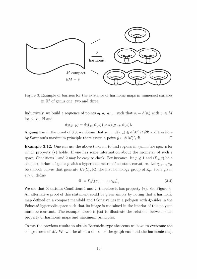
Let us start with the simplest case, the manifold (S2 × S2, g × g) which is isometric to

G+2,4 with its standard metric. By Example 3.6, we know that S2\(1

2Eq)ε has property

(?). We define R :=(S2\(1

2Eq)ε × (S2\(1

2Eq)ε)

)and look at a given geodesic in S2 × S2:

γ :R −→ S2 × S2

t 7→ (γ1(t), γ2(t)).(5.7)

where γ1, γ2 : R −→ S2 are two geodesics in S2. Therefore R satisfies Conditions 1 and

2 of Theorem 3.11 (actually, Theorem 3.3 already suffices to see that R is a barrier) and

therefore R has property (?) as well. (See Figure 4)

By Equation (5.5), if Σ2 = (x, f(x)) is an embedded minimal surface in R4 where

f : R2 −→ R2 is a smooth mapping with slope ∆f < β0 < +∞, then the harmonic Gauss

map γ : Σ2 −→ G+2,4 has its image lying in the above region, i.e., γ(Σ2) ⊂ R. Now, by

Theorem 3.13, we have that γ is constant, implying that Σ2 is a plane in R4.

For the more general case where n = p + 2, we proceed as follows. Let w ∈ G+p,p+2 ⊂

S(p+2p )−1 be written as w = e1 ∧ ...∧ ep, where {ei}pi=1 is an orthonormal basis for Vw and

24

p

A(p)

p

A(p)

Figure 4: (12Eq)ε × (1

2Eq)ε remains as a barrier in S2 × S2.

{n1, n2} an orthonormal basis for V ⊥w . In TwG+p,p+2 there are p(p−1)

2vectors of type 2 (as

∧ anti-commutes), we denote them by X i2, i = 1, ..., p(p−1)

2.

For a given ε > 0, define

R :=

p(p−1)2⋃i=1

( ⋃−tXi2

+ε<t<tXi2−ε

BG(wXi2(t))). (5.8)

Since G+p,p+2 is a homogeneous space of non-negative curvature and the geodesics are

given by Equation (4.28), we have that R satisfies Condition 2 in section 3, that is, for a

given w ∈ R, up to time t < tXj , j = 1, 2, there is always a direction where the distance

to w increases. On the other hand, as we take the union over −tX2 + ε < t < tX2 − ε (i.e.,

strictly smaller than the critical time), we are excluding the points where 〈w,wXi2(t)〉 =

cos2(t/√

2) = 0, therefore 〈w,wXi2(t)〉 > 0 for all i = 1, ..., p(p − 1)/2 and there are no

closed geodesics in R centered at any point w ∈ R. Once more, as G+p,p+2 ⊂ S(p+2

p )−1 is a

symmetric space, w−Xi2(t) = wXi

2(−t), and we have that the only points in wXi

2(R) we

are excluding are the ones that are ε-close to the equator with respect to w in S(p+2p )−1,

thus R =(G+p,p+2\Hem(−w)

)ε

has property (?) and hence, by Theorem 3.13, property

(?) for graphs, for every ε > 0.

Once more, by Equation (5.5), if Mp = (x, f(x)) is an embedded minimal submanifold in

Rp+2 and f is a smooth mapping with slope ∆f < β0 < +∞, then the harmonic Gauss

map γ : Mp −→ G+p,p+2 satisfies γ(Mp) ⊂ R. Thus γ is constant and Mp is a plane in

Rp+2.

25

Remark 5.1. If n ≥ p+ 3, the definition of such a region R would have to include not

only the union over directions of type 3 (and more), but unions over type 2 vectors in

directions of type 1 and so on. For example, once we transport a type 1 vector along a

geodesic with tangent vector of type 3, we may obtain a type 2 vector and hence we have

to control with different arguments whether this would give us a closed geodesic in R. It

can be proven that in general a closed geodesic exists inside R if we take the union over

all directions in higher codimensions. Therefore a more refined definition of such a region

in higher codimension is necessary, as follows from the existence of the Lawson-Osserman

cone.

Returning to codimension 2, the above discussion yields the following theorem, which

extends Moser’s result from codimension 1 to codimension 2.

Theorem 5.2. Let zi = f i(x1, ..., xp), i = 1, 2 be smooth functions defined everywhere in

Rp. Suppose their graph M = (x, f(x)) is a submanifold with parallel mean curvature in

Rp+2. Suppose that there exists a number β0 < +∞ such that

∆f (x) ≤ β0 for all x ∈ Rn, (5.9)

where

∆f (x) :={

det(δαβ +

∑i

f ixα(x)f ixβ(x))} 1

2 . (5.10)

Then f 1, f 2 are linear functions on Rp representing an affine p-plane in Rp+2.

References

[1] William K. Allard, On the first variation of a varifold, Annals of Mathematics 95 (1972), no. 3,

417–491. ↑4, 14

[2] Enrico Bombieri, Ennio De Giorgi, and Enrico Giusti, Minimal cones and the Bernstein problem,

Inventiones mathematicae 7 (1969), no. 3, 243–268. ↑2

[3] Q Chen and YL Xin, A generalized maximum principle and its applications in geometry, American

Journal of Mathematics 114 (1992), no. 2, 355–366. ↑4

[4] Shiing-shen Chern, On the curvatures of a piece of hypersurface in Euclidean space, Abhandlungen

aus dem mathematischen seminar der universitat hamburg, 1965, pp. 77–91. ↑4

[5] James Eells and Luc Lemaire, Two reports on harmonic maps, World Scientific, 1995. ↑4, 7

[6] Doris Fischer-Colbrie, Some rigidity theorems for minimal submanifolds of the sphere, Acta Mathe-

matica 145 (1980), no. 1, 29–46. ↑14

[7] Stefan Hildebrandt, Jurgen Jost, and K-O Widman, Harmonic mappings and minimal submanifolds,

Inventiones mathematicae 62 (1980), no. 2, 269–298. ↑3, 4, 6

26

[8] Jurgen Jost and Yuan-Long Xin, Bernstein type theorems for higher codimension, Calculus of

variations and Partial differential equations 9 (1999), no. 4, 277–296. ↑3, 4, 6, 15

[9] Jurgen Jost, Yuan Long Xin, and Ling Yang, The Geometry of Grassmannian manifolds and

Bernstein type theorems for higher codimension, Annali della Scuola Normale Superiore di Pisa.

Classe di scienze 16 (2016), no. 1, 1–39. ↑3, 4, 6

[10] Jurgen Jost, Yuanlong Xin, and Ling Yang, The regularity of harmonic maps into spheres and

applications to Bernstein problems, Journal of Differential Geometry 90 (2012), no. 1, 131–176. ↑3,

10

[11] Sergey Emel’yanovich Kozlov, Geometry of the real Grassmannian manifolds. Parts I, II and III,

Zapiski Nauchnykh Seminarov POMI 246 (1997), 84–129. ↑15, 21

[12] H Blaine Lawson and Robert Osserman, Non-existence, non-uniqueness and irregularity of solutions

to the minimal surface system, Acta Mathematica 139 (1977), no. 1, 1–17. ↑2

[13] Jurgen Moser, On Harnack’s theorem for elliptic differential equations, Communications on Pure

and Applied Mathematics 14 (1961), no. 3, 577–591. ↑1, 2, 4, 24

[14] Ernst A Ruh and Jaak Vilms, The tension field of the Gauss map, Transactions of the American

Mathematical Society 149 (1970), no. 2, 569–573. ↑3

[15] Joseph H Sampson, Some properties and applications of harmonic mappings (1978). ↑4, 7

[16] James Simons, Minimal varieties in Riemannian manifolds, Annals of Mathematics (1968), 62–105.

↑2, 14

27