The I Theory of Money∗

Markus K. Brunnermeier and Yuliy Sannikov†

September 24, 2015

Abstract

A theory of money needs a proper place for financial intermediaries. Intermediaries

create inside money and their ability to take risks determines the money multiplier. In

downturns, intermediaries shrink their lending activity and fire-sell assets. Moreover,

they create less inside money, exactly at a time when the demand for money rises.

The resulting Fisher disinflation hurts intermediaries and other borrowers. The initial

shock is amplified, volatility spikes and risk premia rise. Monetary policy is redistribu-

tive. An accommodative monetary policy in downturns, focused on the assets held by

constrained agents, recapitalizes balance sheet-impaired sectors and hence mitigates

these destabilizing adverse feedback effects. A monetary policy rule that accommo-

dates negative shocks and tightens after positive shocks provides ex-ante insurance,

mitigates financial frictions, reduces endogenous risk and risk premia, but also creates

moral hazard.

∗We are grateful to comments by discussants Doug Diamond, Mike Woodford, Marco Bassetto and sem-inar participants at Princeton, Bank of Japan, Philadelphia Fed, Rutgers, Toulouse School of Economics,Wim Duisenberg School, University of Lausanne, Banque de France-Banca d’Italia conference, Universityof Chicago, New York Fed, Chicago Fed, Central Bank of Chile, Penn State, Institute of Advanced Studies,Columbia University, University of Michigan, University of Maryland, Northwestern, Cowles General Equi-librium Conference, Renmin University, Johns Hopkins, Kansas City Fed, IMF, LSE, LBS, Bank of England,the Central Bank of Austria, Board of Governors of the Federal Reserve and Harvard University.†Brunnermeier: Department of Economics, Princeton University, markus@princeton.edu, Sannikov: De-

partment of Economics, Princeton University, sannikov@gmail.com

1

1 Introduction

A theory of money needs a proper place for financial intermediaries. Financial institutions are

able to create money – when they extend loans to businesses and home buyers, they credit

the borrowers with deposits and so create inside money. The amount of money created

by financial intermediaries depends crucially on the health of the banking system and the

presence of profitable investment opportunities. This paper proposes a theory of money

and provides a framework for analyzing the interaction between price stability and financial

stability. It therefore provides a unified way of thinking about monetary and macroprudential

policy.

Intermediaries serve three roles. First, intermediaries monitor end-borrowers. Second,

they diversify by extending loans to and investing in many businesses projects and home

buyers. Third, they are active in maturity and liquidity transformation as they issue liquid

short-term (inside) money and invest in illiquid long-term assets. Intermediation involves

taking on some risk. Hence, a negative shock to end borrowers also hits levered intermediary

balance sheets. Intermediaries’ individually optimal response to an adverse shock is to shrink

their balance sheet. They lend less and accept fewer deposits. As a consequence, the amount

of inside money in the economy shrinks. At the same time, because idiosyncratic risk is less

well diversified, demand for money increases. Together, both effects lead to increase in the

value of outside money, i.e. disinflation occurs.

The disinflationary spiral in our model can be understood through two polar cases. In

one polar case the financial sector is undercapitalized and cannot perform its functions. As

the intermediation sector does not create any inside money, money supply is scarce and the

value of money is high. Households have a desire to hold money which, unlike the household’s

own risky individual project, is subject only to aggregate, not idiosyncratic, risk. The value

of safe money is high – indeed, as in Samuelson (1958) and Bewley (1980) it is a bubble. In

the opposite polar case, intermediaries are well capitalized and so well-equipped to mitigate

financial frictions. They are able to exploit diversification benefits by investing across many

different projects. Intermediaries also create short-term (inside) money and hence the money

multiplier is high. At the same time, since households can offload some of their idiosyncratic

risks to the intermediary sector, their demand for money is low. Hence the value of money

is low in this polar case.

As intermediaries are exposed to end-borrowers’ risk, an adverse shock also lowers the

financial sector’s risk bearing capacity. It moves the economy closer to the first polar regime

2

with high value of money. In other words, a negative productivity shock leads to disinfla-

tion a la Fisher (1933). Financial institutions are hit on both sides of their balance sheets.

On the asset side, they are exposed to productivity shocks of their end-borrowers. End-

borrowers’ fire sales depress the price of physical capital and liquidity spirals further erode

intermediaries’ net worth (as shown in Brunnermeier and Sannikov (2014)). On the liabil-

ities side, they are hurt by the Fisher disinflation. As intermediaries cut their lending and

create less inside money, money demand rises and the real value of their nominal liabilities

expands. The Fisher disinflation spiral amplifies the initial shock and the asset liquidity

spiral even further. Overall, the economy’s capacity to diversify idiosyncratic risk moves

around endogenously.

Monetary policy can work against the adverse feedback loops that precipitate crises, by

affecting the prices of assets held by constrained agents and redistributing wealth. That is,

monetary policy works through wealth/income effects, unlike conventional New Keynesian

models in which monetary policy gains traction by changing intertemporal incentives – a

substitution effect. Specifically, in our model, monetary policy softens the blow of negative

shocks and helps to maintain the intermediary sector’s capacity to diversify idiosyncratic

risk. Thus, it reduces endogenous (self-generated) risk and overall risk premia. Monetary

policy is redistributive, but it is not a zero-sum game – it can actually improve welfare.

Simple interest rate cuts in downturns improve economic outcomes only if they boost

prices of assets, such as long-term government bonds, that are held by constrained sectors.

Wealth redistribution towards the constrained sector leads to a rise in economic activity and

an increase in the price of physical capital. As the constrained intermediary sector recovers,

it creates more (inside) money and reverses the disinflationary pressure. The appreciation

of long-term bonds also mitigates money demand, as long-term bonds can be used as a store

of value as well. As banks are recapitalized, they are able to take on more idiosyncratic

household risks, so economy-wide diversification of risk improves and the overall economy

becomes, somewhat paradoxically, safer. In a sense, this like the Keynesian savings paradox

(less individual saving means more aggregate saving), but now applied to risk. Importantly,

monetary policy also affects risk premia. As interest rate cuts affect the equilibrium alloca-

tions, they also affect the long-term real interest rate as documented by Hanson and Stein

(2014) and term premia and credit spread as documented by Gertler and Karadi (2014).

From an ex-ante perspective long-term bonds provide intermediaries with a hedge against

losses due to negative macro shocks, appropriate monetary policy rule can serve as an insur-

ance mechanism against adverse events.

3

Like any insurance, “stealth recapitalization” of the financial system through monetary

policy can potentially create a moral hazard problem. However, moral hazard from monetary

policy is less severe than that associated with explicit bailouts of failing institutions. The

reason is that monetary policy is a crude redistributive tool that helps the strong institutions

more than the weak. The cautious institutions that bought long-term bonds as a hedge

against downturns benefit more from interest rate cuts than the opportunistic institutions

that increased leverage to take on more risk. In contrast, ex-post bailouts of the weakest

institutions create strong risk-taking incentives ex-ante.

To compare various alternative monetary policy rules we develop a full welfare analysis

for our heterogeneous agent model. One might think that a monetary policy rule that fully

removes endogenous risk is the optimal one. However, this is not the case due to pecuniary

externalities – everybody takes the price of physical capital and the price of money as given.

Our analysis shows that investment is excessive and drives up the price of capital beyond

the optimal one, lowering the return of capital. In other words, households take on too much

idiosyncratic risk. A monetary policy that fully removes endogenous risk only partially

completes markets, and so in particular need not be – and in this model is not – welfare-

improving, as in the famous Hart (1975) example. A better policy removes some, but not

all endogenous risk, striking an optimal balance between removing endogenous risk and

leaning against pecuniary externalities. Finally, we show that combining monetary policy

with macroprudential policy measures that limit individual households’ undiversifiable risk-

taking significantly increases welfare.

Related Literature. Our approach differs in important ways from both the prominent

New Keynesian approach but also from the monetarist approach. The New Keynesian ap-

proach emphasizes the interest rate channel. It stresses the role of money as unit of account

and price and wage rigidities are the key frictions. Price stickiness implies that a lowering

nominal interest rates also lowers the real interest rate. Households bring consumption for-

ward and investment projects become more profitable. Within the class of New Keynesian

models, Christiano, Moto and Rostagno (2003) is closest to our analysis as it studies the

disinflationary spiral during the Great Depression. More recently, Curdia and Woodford

(2010) introduced financial frictions in the new Keynesian framework.

In contrast, our I Theory stresses the role of money as store of value and the redistributive

channel of monetary policy. Financial frictions are the key friction. Prices are fully flexible.

This monetary transmission channel works primarily through capital gains, as in the asset

pricing channel promoted by Tobin (1969) and Brunner and Meltzer (1972). As assets are

4

not held symmetrically in our setting, monetary policy redistributes wealth and thereby

mitigates debt overhang problems. In other words, instead of emphasizing the substitution

effect of interest rate changes, the I Theory stresses wealth/income effects of interest rate

changes.

Like in monetarism (see e.g. Friedman and Schwartz (1963)), an endogenous reduction

of money multiplier (given a fixed monetary base) leads to disinflation in our setting. While

inside and outside money have identical return and risk profiles (and so are perfect substitutes

in the eyes of an individual investor), they are not the same for the economy as a whole.

Inside money serves a special function: By creating inside money, intermediaries are able

to diversify risks and foster economic growth. Hence, in our setting monetary intervention

should aim to recapitalize undercapitalized borrowers rather than simply increase the money

supply across the board. A key difference to our approach is that we focus more on the role

of money as a store of value instead of the transaction role of money. The latter plays an

important role in the “new monetarist economics” as outlined in Williamson and Wright

(2011) and references therein.

Instead of the “money view” our approach is closer in spirit to the “credit view” a la

Gurley and Shaw (1955), Patinkin (1965), Tobin (1969, 1970), Bernanke (1983) Bernanke

and Blinder (1988) and Bernanke, Gertler and Gilchrist (1999).1

As in Samuelson (1958) and Bewley (1980), money is essential in our model in the

sense of Hahn (1973). In Samuelson households cannot borrow from future not yet born

generations. In Bewley (1980) and Scheinkman and Weiss (1986) households face explicit

borrowing limits and cannot insure themselves against idiosyncratic shocks. Agents’ desire

to self-insure through precautionary savings creates a demand for the single asset, money.

In our model households can hold money and physical capital. The return on capital is risky

and its risk profile differs from the endogenous risk profile of money. Financial institutions

create inside money and mitigate financial frictions. In Kiyotaki and Moore (2008) money

and capital coexist. Money is desirable as it does not suffer from a resellability constraint as

physical capital does. Lippi and Trachter (2012) characterize the trade-off between insurance

and production incentives of liquidity provision. Levin (1991) shows that monetary policy is

more effective than fiscal policy if the government does not know which agents are productive.

The finance papers by Diamond and Rajan (2006) and Stein (2012) also address the role of

1The literature on credit channels distinguishes between the bank lending channel and the balancesheet channel (financial accelerator), depending on whether banks or corporates/households are capitalconstrained. Strictly speaking our setting refers to the former, but we are agnostic about it and prefer thebroader credit channel interpretation.

5

monetary policy as a tool to achieve financial stability.

More generally, there is a large macro literature which also investigated how macro shocks

that affect the balance sheets of intermediaries or end-borrowers become amplified and affect

the amount of lending and the real economy. These papers include Bernanke and Gertler

(1989), Kiyotaki and Moore (1997) and Bernanke, Gertler and Gilchrist (1999), who study

financial frictions using a log-linearized model near steady state. In these models shocks

to intermediary/end-borrower net worths affect the efficiency of capital allocation and asset

prices. However, log-linearized solutions preclude volatility effects and lead to stable system

dynamics. Brunnermeier and Sannikov (2014) study the full equilibrium (risk) dynamics,

focusing on the differences in system behavior near the steady state, and away from it. They

find that the system is stable to small shocks near the steady state, but large shocks make

the system unstable and generate systemic endogenous risk. Thus, system dynamics are

highly nonlinear. Large shocks have much more serious effects on the real economy than

small shocks. He and Krishnamurthy (2013) also study the full equilibrium dynamics and

focus in particular on credit spreads. In Mendoza and Smith’s (2006) international setting

the initial shock is also amplified through a Fisher debt-disinflation that arises from the

interaction between domestic agents and foreign traders in the equity market. In our paper

debt disinflation is due to the appreciation of inside money. For a more detailed review of

the literature we refer to Brunnermeier et al. (2013).

This paper is organized as follows. Section 2 sets up the model and derives first the solu-

tions for two polar cases. Section 3 presents computed examples and discusses equilibrium

properties, including capital and money value dynamics, the amount of lending through in-

termediaries, and the money multiplier for various parameter values. Section 4 introduces

long-term bonds and studies the effect of interest-rate policies as well as open-market oper-

ations. Section 5 showcases a numerical example of monetary policy. Section 6 concludes.

2 The Baseline Model Absent Policy Intervention

The economy is populated by two types of agents: households and intermediaries. Each

household can use capital to produce either good a or good b, but can only manage a

single project at a time. Each project carries both idiosyncratic and aggregate good-specific

risk. The two goods are then combined into an aggregate good that can be consumed or

invested. Intermediaries help fund households that produce good b by buying their equity.

Intermediaries pool these equity stakes in order to diversify the idiosyncratic risk, and obtain

6

funding for these holdings by accepting money deposits. Households that produce good a

cannot issue equity to intermediaries.

Households can split their wealth between one project of their choice and money. There

is outside money - currency, whose nominal supply is fixed in the absence of monetary policy

- and inside money - currency claims issued by intermediaries to finance their investments

in equity of households that use technology b. However, while the nominal supply of outside

money is fixed, the real value of money is determined endogenously in equilibrium. The

dynamic evolution of the economy is driven by the effect of shocks on the agents’ wealth

distribution, as reflected through their portfolio choice. The model is solved using stan-

dard portfolio choice theory, except that asset prices - including the price of money - are

endogenous.

Technologies. All physical capital Kt in the world is allocated between the two tech-

nologies. If capital share ψt ∈ [0, 1] is devoted to produce good a, then goods a and b

combined make A(ψ)Kt of the aggregate good. Function A(ψ) is concave and has an interior

maximum, an example is the standard technology with constant elasticity of substitution s,2

A(ψ) = A(

1

2ψs−1s +

1

2(1− ψ)

s−1s

) ss−1

.

In competitive markets, prices of goods a and b reflect their marginal contributions to the

aggregate good. Prices must be such that a unit of capital employed in each sector produces

output valued at

Aa(ψ) = (1− ψ)A′(ψ) + A(ψ) and Ab(ψ) = −ψA′(ψ) + A(ψ),

respectively.3

2For s = ∞ the outputs are perfect substitutes, for s = 0 there is no substitutability at all, while fors = 1 the substitutability corresponds to that of a Cobb-Douglas production function.

3If total output is A(ψ)K, then an ε amount of capital devoted to technology a would change totalproductivity to

A

(ψK + ε

K + ε

)(K + ε).

Differentiating with respect to ε at ε = 0, we obtain

A′(ψ)K + ε− (ψK + ε)

(K + ε)2(K + ε) +A(ψ) = A′(ψ)(1− ψ) +A(ψ).

Likewise, the marginal contribution of capital devoted to technology b would be A(ψ)−ψA′(ψ). The weightedsum of the two terms is A(ψ) since the production technology is homogenous of degree 1.

7

Physical capital kt is subject to shocks that depend on the technology in which it is

employed. If used in technology a capital follows

dktkt

= (Φ(ιt)− δ) dt+ σa dZat + σa dZt, (2.1)

where dZat are the sector-wide Brownian shocks and dZt are project-specific shocks, indepen-

dent across agents, which cancel out in the aggregate. A similar equation applies if capital

is used in technology b. Sector-wide shocks dZat and dZb

t are independent of each other. The

investment function Φ has the standard properties Φ′ > 0 and Φ′′ ≤ 0, and the input for

investment ιt is the aggregate good.

Preferences. All agents have identical logarithmic preferences with a common discount

rate ρ. That is, any agent maximizes the expected utility of

E

[∫ ∞0

e−ρt log ct dt

],

subject to individual budget constraints, where ct is the consumption of the aggregate good

at time t.

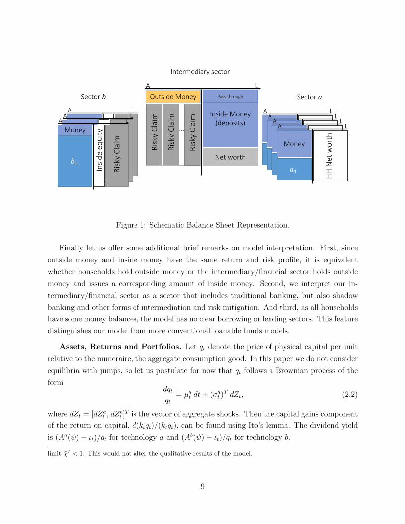
Financing Constraints. Households can hold money and invest in either technology

a or technology b. They can issue risky claims only towards the intermediary sector (not

to each other). However, the amount of risk they can offload to the intermediary sector is

bounded above, with bounds χa and χb satisfying 0 ≤ χa < χb ≤ 1.4 For simplicity, we

set in our baseline model χa = 0, and then denote χ ≡ χb, with χ near 1. Intermediaries

finance their risky holdings (households’ outside equity) by issuing claims (nominal IOUs)

with return identical to the return on money. These claims, or inside money, are as safe

as currency, outside money. In the baseline model, there is a fixed amount of outside fiat

money in the economy that pays zero interest. Figure 1 provides a schematic representation

of the basic financing structure of the model.5

4Notice that if χa = χb, then by holding this maximum fraction of equity of each sector, intermediariesguarantee that the fundamental risk of their assets is proportional to the risk of the economy as a whole. Inthis case, intermediaries end up perfectly hedged, as the risk of money is also proportional to the risk of thewhole economy and the intermediaries’ wealth share follows a deterministic path. In contrast, if χa < χb,then intermediaries are always overexposed to the risk of sector b. In this case, they hold the maximumamount χa of equity of sector a, as this helps them hedge and also helps households in sector a offloadaggregate risk. They also hold more than fraction χa of equity of sector b, as the risk premium they demandis initially second-order, and households in sector b demand insurance.

5The model could be easily enriched to allow intermediaries to sell off part of the equity claims up to a

8

A L

Ris

ky C

laim

A LR

isky

Cla

im…

Net worth

Inside Money(deposits)

A L

Outside Money Pass through

Ris

ky C

laim

Ris

ky C

laim

Ris

ky C

laimA L

𝑏1

Money

Ris

ky C

laim

Insi

de

equ

ity

A LA L

A LA L

𝑎1

Money

HH

Net

wo

rth

Intermediary sector

Sector 𝑎Sector 𝑏

Figure 1: Schematic Balance Sheet Representation.

Finally let us offer some additional brief remarks on model interpretation. First, since

outside money and inside money have the same return and risk profile, it is equivalent

whether households hold outside money or the intermediary/financial sector holds outside

money and issues a corresponding amount of inside money. Second, we interpret our in-

termediary/financial sector as a sector that includes traditional banking, but also shadow

banking and other forms of intermediation and risk mitigation. And third, as all households

have some money balances, the model has no clear borrowing or lending sectors. This feature

distinguishes our model from more conventional loanable funds models.

Assets, Returns and Portfolios. Let qt denote the price of physical capital per unit

relative to the numeraire, the aggregate consumption good. In this paper we do not consider

equilibria with jumps, so let us postulate for now that qt follows a Brownian process of the

formdqtqt

= µqt dt+ (σqt )T dZt, (2.2)

where dZt = [dZat , dZ

bt ]T is the vector of aggregate shocks. Then the capital gains component

of the return on capital, d(ktqt)/(ktqt), can be found using Ito’s lemma. The dividend yield

is (Aa(ψ)− ιt)/qt for technology a and (Ab(ψ)− ιt)/qt for technology b.

limit χI < 1. This would not alter the qualitative results of the model.

9

The total (real) return of an individual project in technology a is

drat =Aa(ψt)− ιt

qtdt+

(Φ(ιt)− δ + µqt + (σqt )

Tσa1a)dt+ (σqt + σa1a)T dZt + σa dZt,

where 1a is the column coordinate vector with a single 1 in position a. The (real) return in

technology b is written analogously. The optimal investment rate ιt, which maximizes the

return of any technology, is given by the first-order condition 1/qt = Φ′(ιt). We denote the

investment rate that satisfies this condition by ι(qt).

The return on technology b is split between households who hold inside equity and earn

drbHt and intermediaries who hold outside equity and earn drbIt , so

drbt = (1− χt) drbHt + χt drbIt ,

where χt ≤ χ is the fraction of outside equity households issue. The two types of equity

have identical risks, but potentially different returns. The required return on inside equity

may be higher if households would like to issue more outside equity but cannot due to the

constraint. That is, in equilibrium we have we have drbHt ≥ drbIt , with equality if χt < χ.

Total money supply is fixed absent monetary policy. The value of all money depends on

the size of the economy. Denote the real value of all outside money by ptKt. Since inside

money is a liability for the intermediary sector and an asset for the household sector, it nets

out overall. Let us postulate that pt follows a Brownian process of the form

dptpt

= µpt dt+ (σpt )T dZt. (2.3)

The law of motion of aggregate capital is

dKt

Kt

= (Φ(ιt)− δ) dt+ ψtσa dZa

t + (1− ψt)σb dZbt︸ ︷︷ ︸

(σKt )T dZt

, (2.4)

and the return on money, the real interest rate, is given just by the capital gains rate

drMt =d(ptKt)

ptKt

=(Φ(ιt)− δ + µpt + (σpt )

TσKt)dt+ (σKt + σpt )

T dZt︸ ︷︷ ︸(σMt )T dZt

.

10

When a household chooses to produce good a, its net worth follows

dntnt

= xat drat + (1− xat ) drMt − ζat dt, (2.5)

where xat is the portfolio weight on capital and ζat is its propensity to consume (i.e. con-

sumption per unit of net worth).

The net worth of a household who produces good b follows

dntnt

= xbt drbHt + (1− xbt) drMt − ζbt dt. (2.6)

Households can choose whether to work in sector a or b, that is, in equilibrium they must

be indifferent with respect to this choice. Denote by αt the net worth of households who

specialize in sector a, as a fraction of total household net worth.

The net worth of an intermediary follows

dntnt

= xt drbIt + (1− xt) drMt − ζt dt, (2.7)

where rbIt denotes the return on households’ outside equity drbIt with idiosyncratic risk di-

versified away, i.e. removed. If intermediaries use leverage, i.e. issue inside money, then of

course xt > 1.

Equilibrium Definition. The agents start initially with some endowments of capital

and money. Over time, they trade - they choose how to allocate their wealth between the

assets available to them. That is, they solve their individual optimal consumption and

portfolio choice problems to maximize utility, subject to the budget constraints (2.5), (2.6)

and (2.7). Individual agents take prices as given. Given prices, markets for capital, money

and consumption goods have to clear.

If the net worth of intermediaries is Nt, then given the world wealth of (qt + pt)Kt, the

intermediaries’ net worth share is denoted by

ηt =Nt

(qt + pt)Kt

. (2.8)

Definition. Given any initial allocation of capital and money among the agents, an

equilibrium is a map from histories {Zs, s ∈ [0, t]} to prices pt and qt, return differential

drbHt − drbIt ≥ 0, the households’ wealth allocation αt, equity allocation χt ≤ χ, portfolio

11

weights (xat , xbt , x) and consumption propensities (ζat , ζ

bt , ζt), such that

(i) all markets, for capital, equity, money and consumption goods, clear,

(ii) all agents choose technologies, portfolios and consumption rates to maximize utility

(households who produce good b also choose χt).

One important choice here is that of households: each household can run only one project

either in technology a or b. They must be indifferent between the two choices. Households

who choose to produce good b must also choose how much equity to issue. If outside equity

earns less than the return of technology b, these households would want to issue the maximal

amount of outside equity of χt = χ. This happens in equilibrium only if intermediaries are

willing to accept this supply of equity at a return discount, i.e. drbIt < drbt , so that inside

equity earns a premium. This is the case only if the intermediaries are well-capitalized.

Otherwise, drbHt = drbIt = drbt , i.e. inside and outside equity of technology b earns the same

return as technology b. In this case, households are indifferent with respect to the amount

of equity they issue, so the equity issuance constraint does not bind.

2.1 Equilibrium Conditions

Logarithmic utility has two well-known tractability properties. First, an agent with loga-

rithmic utility and discount rate ρ consumes at the rate given by ρ times net worth. Thus,

ζt = ζat = ζbt = ρ and the market-clearing condition for consumption goods is

ρ(qt + pt)Kt = (A(ψt)− ιt)Kt. (2.9)

Second, the excess return of any risky asset over any other risky asset is explained by the

covariance between the difference in returns and the agent’s wealth.

From (2.5) and (2.6), the wealth of households in sectors a and b is exposed to aggregate

risk of

σNat = xat(σa1a + σqt − σMt

)︸ ︷︷ ︸νat

+σMt and σNbt = xbt(σb1b + σqt − σMt

)︸ ︷︷ ︸νbt

+σMt ,

and idiosyncratic risk of xat σa and xbt σ

b, respectively. Consequently, the difference between

12

expected returns of technology a and money is given by

Et[drat − drMt ]

dt= (νat )TσNat + xat (σ

a)2, (2.10)

where the right-hand side is the covariance of the net worth of a household in sector a with

the excess risk of technology a over money.

To write an analogous condition for technology b, we have to take into account the split

of risk between households and intermediaries. Note that the net worth of intermediaries is

exposed to risk

σNt = xtνbt + σMt .

Therefore, the expected excess return of technology b must satisfy

Et[drbt − drMt ]

dt= (1− χt)((νbt )TσNbt + xbt(σ

b)2) + χt(νbt )TσNt (2.11)

The difference in return of inside and outside equity of households in sector b is then

drbHt − drbItdt

= (νbt )TσNbt + xbt(σ

b)2 − (νbt )TσNt ≥ 0,

with equality if χt < χ.

Households must be indifferent between investing in technologies a and b. The following

proposition summarizes the relevant condition

Proposition 1. In equilibrium

(xat )2(|νat |2 + (σa)2) = (xbt)

2(|νbt |2 + (σb)2). (2.12)

Proof. See Appendix.

Market clearing for capital implies that portfolio weights, given the net worth shares of

intermediaries and households, have to be consistent with the allocation of the fraction ψt

of capital to technology b. Denote by

ϑt =pt

qt + pt

13

the fraction of the world wealth that is in the form of money. Then

xt =χtψt(1− ϑt)

ηt. (2.13)

Furthermore, the net worth of households who employ technologies a and b, together, must

add up to 1− ηt, i.e.,

(1− ψt)(1− ϑt)xat

+ψt(1− χt)(1− ϑt)

xbt= 1− ηt, (2.14)

and the fraction household wealth in sector a is given by

αt =(1− ψt)(1− ϑt)xat (1− ηt)

.

2.2 Evolution of the State Variable

Finally, we have to describe how the state variable ηt, which determines prices of capital and

money pt and qt, evolves over time. The law of motion of ηt, together with the specification

of prices and allocations as functions of ηt, constitute the full description of equilibrium: i.e.

the map from any initial allocation and a history of shocks {Zs s ∈ [0, t]} into the description

of the economy at time t after that history. The following proposition characterizes the

equilibrium law of motion of ηt.

Proposition 2. The equilibrium law of motion of ηt is given by

dηtηt

= (1− ηt)(x2t |νbt |2 − (xat )

2(|νat |2 + (σa)2))dt+ (xtν

bt + σϑt )T (σϑt dt+ dZt). (2.15)

The law of motion of ηt is so simple because the earnings of intermediaries and households

can be expressed in terms of risks they take and the required equilibrium risk premia. The

first term on the right-hand side reflects the relative earnings of intermediaries and house-

holds. The second term on the right-hand side of (2.15) reflects mainly the volatility of ηt,

due to the imperfect risk sharing between intermediaries and households.

Proof. The law of motion of total net worth of intermediaries, given the risks that they take,

14

must bedNt

Nt

= drMt − ρ dt+ xt(νbt )T ((xtν

bt + σMt )︸ ︷︷ ︸σNt

dt+ dZt). (2.16)

The law of motion of world wealth (qt + pt)Kt, the denominator of (2.8), can be found from

the total return on world wealth, after subtracting the dividend yield of ρ (i.e., aggregate

consumption). To find the returns, we take into account the risk premia that various agents

earn. We have

d((qt + pt)Kt)

(qt + pt)Kt

= drMt − ρ dt+ (1− ϑt) (σKt + σqt − σMt )T︸ ︷︷ ︸(σqt−σ

pt )T

dZt+

(1− ϑt)((1− ψt) ((νat )TσNat + xat (σa)2)︸ ︷︷ ︸

Et[drat −dr

Mt ]

dt

+ψt(χt(ν

bt )TσNt + (1− χt)((νbt )TσNbt + xbt(σ

b)2))︸ ︷︷ ︸

Et[drbt−dr

Mt ]

dt

) dt.

Recall that

σNt = xtνbt + σMt , σNat = xat νt + σMt and σNbt = xbtν

bt + σMt

and note that

(1− ψt)νat + ψtνbt = σqt − σ

pt .

Therefore, the law of motion of aggregate wealth can be written as6

d((qt + pt)Kt)

(qt + pt)Kt

= drMt − ρ dt+ (1− ϑt)(σqt − σpt )T︸ ︷︷ ︸

−(σϑt )T

(σMt dt+ dZt)+

(1− ϑt)((1− ψt)xat (|νat |2 + (σa)2) + ψt

(χtxt|νbt |2 + (1− χt)xbt(|νbt |2 + (σb)2)

))dt =

drMt − ρ dt− (σϑt )T (σMt dt+ dZt) + ηt x2t |νbt |2 dt+ (1− ηt)(xat )2(|νat |2 + (σa)2) dt, (2.17)

where we used (2.14) and the indifference condition of Proposition 1.

Thus, using Ito’s lemma, we obtain (2.15).7

6Ito’s lemma implies that σϑt = (1− ϑ)(σpt − σqt ) and µϑt = (1− ϑ)(µpt − µ

qt )− σϑσp + (σϑ)2.

7If processes Xt and Yt follow

dXt/Xt = µXt dt+ σXt dZt and dYt/Yt = µYt dt+ σYt dZt,

15

3 Model without Intermediaries

The goal of this section is to understand the determinants of the value of money in a model

without intermediaries. The key determinant of the value of money is, of course, the level

of idiosyncratic risk.

We can anticipate properties of full equilibrium dynamics through our understanding of

the economy without intermediaries. Since intermediaries reduce the amount of idiosyncratic

risk in the economy, the presence of a healthy intermediary sector is akin to a reduction in

idiosyncratic risk parameters in the model without intermediaries.

3.1 Value and Risk of Money

Assume that η = 0. Suppose for the sake of simplicity that σa = σb = σ, σa = σb = σ and

that maxψ A(ψ) = A is maximized at ψ = 1/2. Then half of all households produce good a,

and the rest, good b. Aggregate capital in the economy follows

dKt

Kt

= (Φ(ιt)− δ) dt+σ

2dZa

t +σ

2dZb

t .

Prices p and q are constant. The volatility of the money (or the whole economy) and the

incremental risk of a project in either sector (orthogonal to the risk of money) are

σ ≡√σ2/2 and σ ≡

√σ2 + σ2/2,

respectively. Note that the total risk of technology a or b is√σ2 + σ2 =

√σ2 + σ2.

Effectively, the economy is equivalent to a single-good economy with aggregate risk σ

and project-specific risk σ. In this economy, the market-clearing condition for output (2.9)

becomes

A− ι(q) = ρ (p+ q)︸ ︷︷ ︸q/(1−ϑ)

. (3.1)

Each household puts portfolio weight 1−ϑ on capital, so its net worth is exposed to aggregate

risk σ and project-specific risk (1 − ϑ)σ. The excess return on capital over money is the

dividend yield (A− ι(q))/q, since the capital gains rates are the same. Therefore, the asset-

thend(Xt/Yt)

Xt/Yt= (µXt − µYt ) dt+ (σXt − σYt )T (dZt − σYt dt).

16

pricing condition of capital relative to money is

A− ι(q)q

= (1− ϑ)σ2 ⇒ ϑ = 1−√ρ/σ. (3.2)

Equilibrium in which money has positive value exists only if σ2 > ρ. As σ increases, the

value of money relative to capital rises.

For a special form of the investment function Φ(ι) = log(κι + 1)/κ, we can also get

closed-form expressions for the equilibrium prices of money and capital.8 Then (3.1) implies

that

q =κA+ 1

κ√ρσ + 1

and p =σ −√ρ√ρ

q. (3.3)

There is always an equilibrium in which money has no value. In that equilibrium the

price of capital satisfies A− ι(q) = ρq, so that

q =κA+ 1

κρ+ 1. (3.4)

Then the dividend yield on capital is (A − ιt)/q = ρ and expected return on capital is

ρ + Φ(ιt) − δ. Subtracting the idiosyncratic risk premium of σ2 the required return on an

asset that carries the same risk as the whole economy, or Kt, is

ρ− σ2 + Φ(ιt)− δ.

If this rate is lower than the growth rate of the economy, i.e. Φ(ιt)− δ, then an equilibrium

in which money has positive value exists. Lemma 1 in the Appendix generalizes these results

to the case when σa 6= σb and σa 6= σb.

These closed-form solutions allow us to anticipate how the value of money may fluctuate

in an economy with intermediaries. When ηt approaches 0, households face high idiosyncratic

risk in both sectors, leading to a high value of money. In contrast, when ηt is large enough,

then most of idiosyncratic risk is concentrated in sector a, as households in sector b pass on

the idiosyncratic risk to intermediaries. This leads to a lower value of money.

Intermediary net worth and the value of money will generally fluctuate due to aggregate

shocks Za and Zb. Relative to world wealth - recall that ηt measures the intermediary net

8When the investment adjustment cost parameter κ is close to 0, i.e. Φ(ι) is close to 1, then the price ofcapital q is goes to 1 (this is Tobin’s q). As κ becomes large, the price of capital depends on dividend yieldA relative to the discount rate ρ and the level of idiosyncratic risk that affects the value of money.

17

worth relative to total wealth - intermediaries are long shocks Zb and short shocks Za when

they invest in equity of households who produce good b. A fundamental assumption of our

model is that intermediaries cannot hedge this aggregate risk exposure. Due to this, they

may suffer losses, and losses force them to stop investing in equity of households who use

technology b. The intermediary sector may become undercapitalized.

Impossibility of “As If” Representative Agent Economies. Note that it is impos-

sible to construct an “as if” representative agent economy with the same aggregate output

and investment streams and same asset prices that mimics the equilibrium outcome of our

heterogeneous agents economy. In any representative agent economy, absence of individual-

level idiosyncratic risk, capital returns strictly dominate money and hence money could never

have some positive value.

3.2 Welfare Analysis

We start with a general result, which allows us to compute welfare of agents with logarithmic

utility. Expression (3.6) below is valid for an arbitrary process (3.5), regardless of whether

it arises from a feasible equilibrium trading strategy or not.9

Proposition 3. Consider an agent who consumes at rate ρnt where nt follows

dntnt

= µnt dt+ σnt dZt (3.5)

Then the agent’s expected future utility at time t takes the form

Et

[∫ ∞t

e−ρ(s−t) log(ρns) ds

]=

log(ρnt)

ρ+

1

ρEt

[∫ ∞t

e−ρ(s−t)(µns −

|σns |2

2

)ds

]. (3.6)

Proof. See Appendix.

Without intermediaries, drift and volatility of wealth for all households are time-invariant.

In general, given portfolio weights 1− ϑ on capital and ϑ on money, we have

µn = (1− ϑ)A− ι(q)

q+ Φ(ι(q))− δ − ρ, σn =

√(1− ϑ)2σ2 + σ2. (3.7)

9For example, we can use (3.5) to evaluate welfare of a hypothetical representative agent, who consumesa portion of world output, to estimate welfare that could be attained without idiosyncratic risk.

18

For the equilibrium value of ϑ given by (3.2), we have

µn = Φ(ι(q))− δ and σn =√ρ+ σ2. (3.8)

Combining (3) with (3.8), we get the following proposition

Proposition 4. Suppose σ2 > ρ, so that monetary equilibrium exists in the economy without

intermediaries. Then in this equilibrium, the welfare of a household with initial wealth n0 = 1

is

UH =log(ρ)

ρ+

Φ(ι(q))− δ − (ρ+ σ2)/2

ρ2.

Macro-prudential regulation. How does welfare in equilibrium with money compare

to welfare in the money-less equilibrium? If the regulator can control the value of money by

specifying a money holding requirement of the agents, will the money under optimal policy

have greater value than in equilibrium, or lower value? Note that higher value of money

allows agents to reduce their idiosyncratic risk exposure, but creates a distortion on the

investment front, since the value of capital becomes lower.

What if the regulator can control ϑ by forcing the agents to hold specific amounts of

money? As it turns out, under some mild restrictions on ϑ, it will be optimal for the planner

to force agents to hold more money. Our results are summarized in the following proposition.

Proposition 5. Assume that Φ(ι) = log(κι+ 1)/κ. Then if money can have positive equilib-

rium value, welfare in equilibrium with money is always greater than that in the moneyless

equilibrium. Furthermore, relative to the value of ϑ in the equilibrium with money, optimal

policy raises ϑ if and only if

σ(1− κρ) < 2√ρ. (3.9)

Proof. See Appendix.

Condition (3.9) reflects the trade-off between the role of money as an insurance asset, and

the distortionary effect of rising money value on investment. On the one hand, the returns

to money are free of idiosyncratic risk, so individual households have less exposure to their

own individual-specific shocks, improving welfare. On the other hand, in the money equilib-

rium, the price of capital is lower, so investment is lower, so overall growth is lower. When

adjustment costs κ are large enough, these distortions are minimal, so the diversification

benefit dominates, as we see in condition (3.9).

19

4 Analysis with Intermediaries

In this section, we analyze the full model economy with intermediaries. Intermediaries are di-

versifiers, allowing households that invest in technology b to offload some of their idiosyncratic

risk. The capacity of intermediaries to act as “diversifiers” depends on their capitalization,

and so it is not surprising that aggregate economic activity also depends on intermediary

capitalization. Since intermediaries are exposed (in a levered way) to the idiosyncratic risk of

technology b, their wealth share moves over time, as different a-shocks and different b-shocks

hit the economy.

In the previous section, we considered the extreme polar case when intermediary capi-

talization is 0. In that case, in the money equilibrium, the value of money is high – it is

an attractive insurance vehicle for households invested in either of the two technologies. In

contrast, with a functioning intermediary sector, households that invest in technology b can

offload some of their idiosyncratic risk, so there is less demand for insurance vehicles. As a

result money is less attractive and so its real value is low. At the other end of the spectrum,

ηt can, however, also be too high: When ηt is close to 1 there is too much focus on the sector

b good and so aggregate economic activity declines.

The rest of this section proceeds as follows. First, we provide a full characterization of

the equilibrium of our economy. Second, we conduct welfare analysis.

4.1 Equilibrium

The computational procedure we employ, both with and without monetary policy, is de-

scribed in Appendix . . . . Consider parameter values ρ = 0.05, A = 0.5 σa = σb = 0.4,

σa = 0.6, σb = 1.2, s = 0.8, Φ(ι) = log(κι+ 1)/κ with κ = 2, and χ = 0.999.

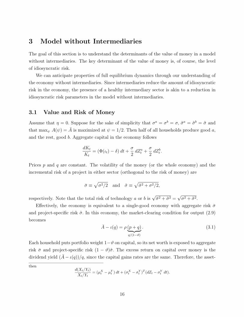
We start by looking at the allocation of capital. The production of good b depends on

intermediaries, it increases in the net worth share of the intermediary sector η. When η drops,

the risk premia that intermediaries demand for equity stakes in projects of households in

sector b rise, to the point that the households may be willing to sell less than fraction χ of

outside equity. See Figure 2.

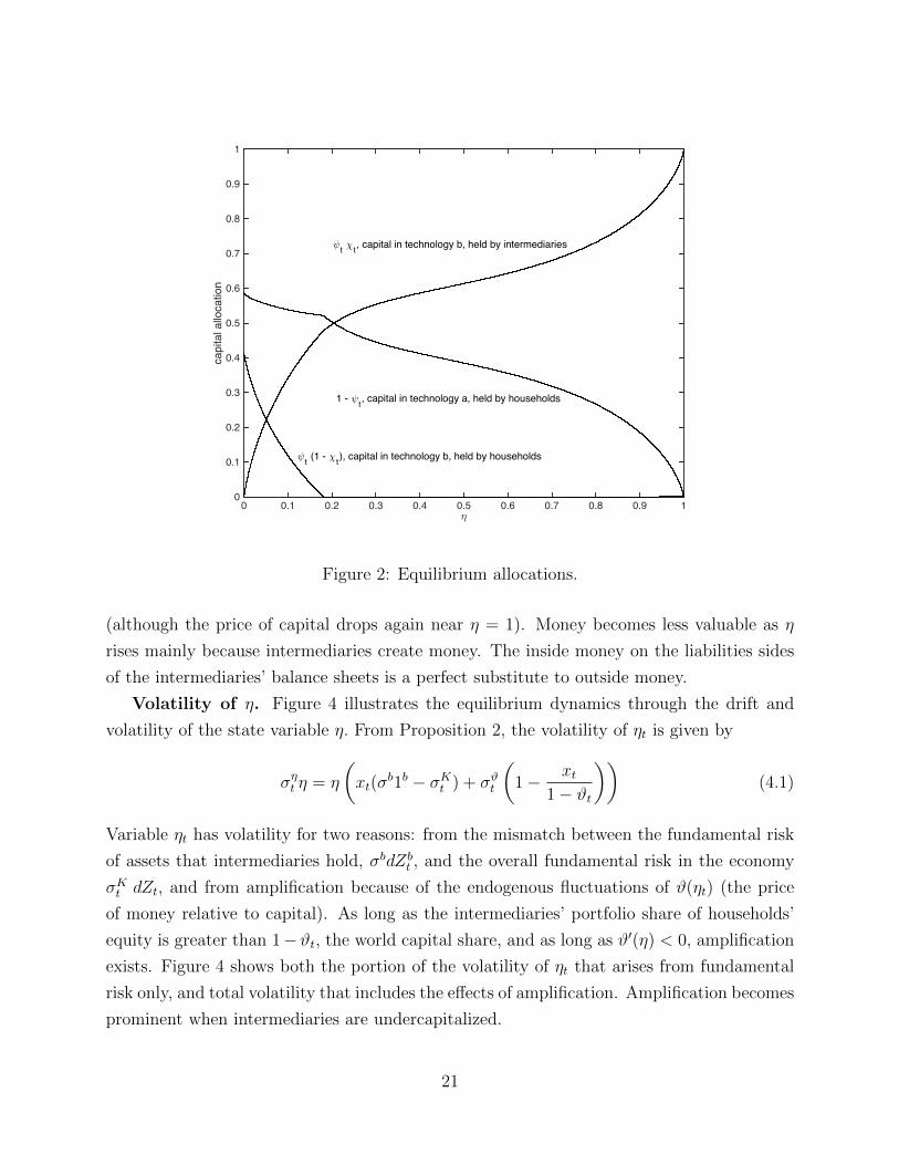
Figure 3 shows the prices p(η) and q(η) of money and capital in equilibrium. At η = 0,

the values of p and q converge to those under the benchmark without intermediaries, q =

1.0532 and p = 3.4151. As η rises, the price of capital rises and the price of money drops

20

�0 0.1 0.2 0.3 0.4 0.5 0.6 0.7 0.8 0.9 1

capi

tal a

lloca

tion

0

0.1

0.2

0.3

0.4

0.5

0.6

0.7

0.8

0.9

1

�t � t , capital in technology b, held by intermediaries

�t (1 - � t), capital in technology b, held by households

1 - �t , capital in technology a, held by households

Figure 2: Equilibrium allocations.

(although the price of capital drops again near η = 1). Money becomes less valuable as η

rises mainly because intermediaries create money. The inside money on the liabilities sides

of the intermediaries’ balance sheets is a perfect substitute to outside money.

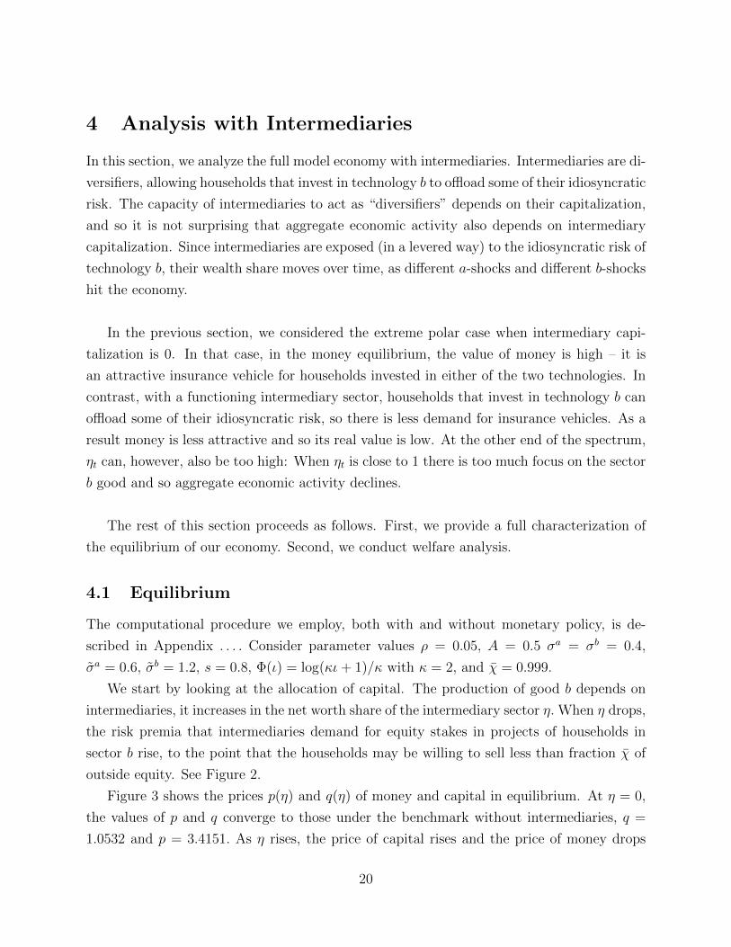
Volatility of η. Figure 4 illustrates the equilibrium dynamics through the drift and

volatility of the state variable η. From Proposition 2, the volatility of ηt is given by

σηt η = η

(xt(σ

b1b − σKt ) + σϑt

(1− xt

1− ϑt

))(4.1)

Variable ηt has volatility for two reasons: from the mismatch between the fundamental risk

of assets that intermediaries hold, σbdZbt , and the overall fundamental risk in the economy

σKt dZt, and from amplification because of the endogenous fluctuations of ϑ(ηt) (the price

of money relative to capital). As long as the intermediaries’ portfolio share of households’

equity is greater than 1−ϑt, the world capital share, and as long as ϑ′(η) < 0, amplification

exists. Figure 4 shows both the portion of the volatility of ηt that arises from fundamental

risk only, and total volatility that includes the effects of amplification. Amplification becomes

prominent when intermediaries are undercapitalized.

21

�0 0.1 0.2 0.3 0.4 0.5 0.6 0.7 0.8 0.9 1

q, p

1

1.5

2

2.5

3

p

q

Figure 3: Equilibrium prices of capital and money.

Liquidity and Disinflationary Spiral. Intermediaries’ wealth share volatility is ampli-

fied by two adverse feedback loops/spirals when η is low. First, the traditional amplification

channel works on the asset sides of the intermediary balance sheets: as the price of physical

capital q(η) drops following a negative shock. Second, shocks hurt intermediaries on the

liability side of the balance sheets through the Fisher disinflationary spiral. The real value

of intermediaries’ liabilities rises. Both effects impair intermediaries’ net worth. Interme-

diaries’ response to these losses is to shrink their balance sheet further, which leads to yet

more fire-sales (lowering the price q) and reduction in inside money (increasing the value

of liabilities p). In other words, they take fewer deposits, create less inside money, and the

money multiplier collapses.10 This again reduces their net worth, and so on.

By rewriting equation (4.1), we can find a mathematical representation of these spirals

in our model.

σηt =xt(σ

b1b − σKt )

1−(ψtχt−ηt

ηt

)−ϑ′(ηt)ϑ/ηt

The numerator reflects the amount of fundamental risk the intermediary sector is exposed

10In reality, rather than turning savers away, financial intermediaries might still issue demand depositsand simply park the proceeds with the central bank as excess reserves.

22

to. The denominator (1 − ...) comes from the sum of a geometric series, a mathematical

manifestation of the spiral. The term ψtχt−ηtηt

corresponds to the intermediary sector’s lever-

age ratio, while ϑ′(η)ϑ/η

is the elasticity of ϑ(·) w.r.t. the wealth share η. The formula clearly

shows that amplification increases with intermediaries’ leverage and with the elasticity (in

a multiplicative fashion). The function ϑ(η) = p(η)/(q(η) + p(η)) subsumes these two spi-

rals. The liquidity spiral works through q(η), while the disinflationary spiral works through

p(η). Figure 3 shows that both spirals are adverse: a negative shock that lowers η lowers

the value of assets q(η), the liquidity spiral, and increases the value of liabilities p(η), the

disinflationary spiral.

�0 0.1 0.2 0.3 0.4 0.5 0.6 0.7 0.8 0.9 1

� ��, |� ��|

-0.04

-0.02

0

0.02

0.04

0.06

0.08 |� �t�|, volatility in equilibrium

� � t�, drift in equilibrium

fundamental portion of equilibrium volatility

Figure 4: Equilibrium dynamics.

Drift of η. The drift of ηt is given by

µηt η = η(1− η)(x2t |νbt |2 − (xat )

2(|νat |2 + (σa)2))

+ ηt(xtνbt + σϑt )Tσϑt (4.2)

The first term captures the relative risk premia that intermediaries and households earn on

their portfolios relative to money. As intermediaries become undercapitalized, the price of

and return from producing good b rises, leading intermediaries to take on more risk. The

opposite happens when intermediaries are overcapitalized - then the price of good a and the

23

households’ rate of earnings rises. The stochastic steady state of ηt is the point where the

drift of ηt equals zero - at that point the earnings rates of intermediaries and households

balance each other out.

The dynamics in Figure 4, together with prices and allocations as functions of η in Figures

2 and 3 characterize the behavior of the economy in equilibrium.

4.2 Inefficiencies and Welfare

In this section, we calculate welfare in our model. Before we proceed, let us briefly describe

the sources of inefficiency. In the process, we would like to emphasize relevant trade-offs

with the intention of preparing ground for thinking about policy. First, there is inefficient

sharing of idiosyncratic risk. Some of it can be mitigated through the use of intermediaries

who can hold equity of households producing good b and diversify some of idiosyncratic risk.

Consequently, cycles that can cause intermediaries to be undercapitalized can be harmful.

Inefficiencies connected with idiosyncratic risks are also mitigated with the use of money -

both inside and outside. Money allows households to diversify their wealth, but high value

of money results in lower price of capital and potential inefficiency due to underinvestment.

Second, there is inefficient sharing of aggregate risk, which can cause whole sectors to

become undercapitalized, e.g. intermediaries. If intermediaries become undercapitalized,

barriers to entry into the intermediary sector help the intermediaries: the price of good b rises

when ηt is low, mitigating the intermediaries risk exposures and allowing the intermediaries

to recapitalize themselves. Thus, the limited competition in the intermediary sector creates

a terms-of-trade hedge, which depends on the extent to which intermediaries cut back the

financing of households in sector b, the extent to which those households are willing to

self-finance, and the substitutability s among the intermediate goods.

Finally, there is productive inefficiency: when intermediaries or households are undercap-

italized, then production may be inefficiently skewed towards good a or good b. Even at the

steady state production can be inefficient due to financial frictions, e.g. imperfect sharing of

idiosyncratic risks.

To understand the cumulative effect of all these inefficiencies, one needs a proper welfare

measure. Welfare analysis is complicated by heterogeneity. We cannot focus on a repre-

sentative household, since different households are exposed to different idiosyncratic risks.

Some households become richer, while others become poorer.

Welfare Calculation. Recall that, according to Proposition 3, for a general wealth

24

process welfare is given by (3.6). We will use this expression to calculate the welfare of

intermediaries, households, as well as a fictitious “representative agent” who consumes a fixed

portion of aggregate output. Intermediaries and households are the focus of our analysis,

while the representative agent is a useful auxiliary construct.

Proposition 6. Welfare of a representative agent with net worth nt = (pt + qt)Kt is given

by

log(ρnt)

ρ− log(pt + qt)

ρ︸ ︷︷ ︸log(ρKt)

ρ

+1

ρEt

[∫ ∞t

e−ρ(s−t)(

log(ps + qs) + Φ(ιs)− δ −|σKs |2

2

)ds

]. (4.3)

Proof. By (3.6), the welfare of an agent who consumes ρKt is given by

Et

[∫ ∞t

e−ρ(s−t) log(ρKs) ds

]=

log(ρKt)

ρ+

1

ρEt

[∫ ∞t

e−ρ(s−t)(

Φ(ιs)− δ −|σKs |2

2

)ds

].

Since log(ρ(ps + qs)Ks) = log(ρKs) + log(ps + qs), we find that the utility of a representative

agent with net worth ρ(pt + qt)Kt is given by (4.3).

Besides being an interesting benchmark, as a welfare measure that excludes the effects

of idiosyncratic risk, measure (4.3) can be adjusted to quantify the welfare of intermediaries

and households.

Proposition 7. The welfare of an intermediary with wealth nIt is log(ρnIt )/ρ+U I(ηt), where

U I(ηt) = − log(ηt(pt + qt))

ρ+

1

ρEt

[∫ ∞t

e−ρ(s−t)(

log(ηs(ps + qs)) + Φ(ιs)− δ −|σKs |2

2

)ds

].

The welfare of a household with net worth nHt is log(ρnHt )/ρ+ UH(η), where

UH(ηt) = − log(pt + qt)

ρ+

1

ρEt

[∫ ∞t

e−ρ(s−t)(

log(ps + qs) + Φ(ιs)− δ −|σKs |2

2

)ds

]+

1

ρEt

[∫ ∞t

e−ρ(s−t)(ηs ((xas)

2(|νas |2 + (σa)2)− x2s|νbs|2) +

|σϑs |2 − (xas)2(|νas |2 + (σa)2)

2

)ds

].

25

Proof. Since intermediary with net worth nIt = ηt(pt + qt)Kt consumes

log(ρηs(ps + qs)Ks) = log(ηs) + log(ρ(ps + qs)Ks),

receiving the same utility flow as a representative household plus log(ηs), we can obtain the

welfare of an intermediary from (4.3) and obtain

log(ρKt)

ρ+

1

ρEt

[∫ ∞t

e−ρ(s−t)(

log(ηs(ps + qs)) + Φ(ιs)− δ −|σKs |2

2

)ds

].

Since log(ρKt) = log(ρnIt )− log(ηt(pt + qt)), we obtain the desired expression.

To compute the welfare of households, notice that by Proposition 3, if two agents have

wealth processes

dntnt

= µnt dt+ σnt dZt anddn′tn′t

= µn′

t dt+ σn′

t dZt,

then the difference in their utility is

log(ρn′t)− log(ρnt)

ρ+

1

ρEt[∫ ∞

t

e−ρ(s−t)(µn′

s − µns +|σns |2 − |σn

′s |2

2

)ds

](4.4)

We can now obtain household utility by adjusting the utility of a representative agent.

Recall that households are indifferent between technologies a and b, so we can focus on

households who use technology a without loss of generality. According to (2.17), world

wealth follows

dntnt

= drMt − ρ dt− (σϑt )T (σMt dt+ dZt) + ηt x2t |νbt |2 dt+ (1− ηt)(xat )2(|νat |2 + (σa)2) dt,

while the net worth of a household that uses technology a follows

dnHtnHt

= drMt − ρ dt+ xat ((νat )T (σNat dt+ dZt) + xat (σ

a)2 dt+ σa dZt)︸ ︷︷ ︸xat ((νat )T (σMt dt+dZt)+σa dZt)+(xat )2(|νat |2+(σa)2) dt

Hence,

µnH

t − µnt = ηt ((xat )2(|νat |2 + (σa)2)− x2

t |νbt |2) + (xat νat + σϑt )TσMt ,

26

|σns |2 − |σnH

s |2

2=|σMt − σϑt |2 − |σMt + xat ν

at |2 − (xat )

2(σa)2

2and so

µnH

t − µnt +|σns |2 − |σn

H

s |2

2= ηt ((xat )

2(|νat |2 + (σa)2)− x2t |νbt |2) +

|σϑt |2 − (xat )2(|νat |2 + (σa)2)

2

Thus, using (4.3) and (4.4) to value the welfare of households, we obtain the desired

expression.

This completes the derivation of the relevant welfare formulae. To then actually com-

pute intermediary and household welfare, it suffices to note that all included quantities are

functions of the single state variable ηt, and that in general

g(ηt) = Et

[∫ ∞t

e−ρ(s−t)y(ηs) ds

]⇒ ρg(η) = y(η) + g′(η)µηt η +

g′′(η)|ησηt |2

2

The actual computation of welfare levels thus merely requires us to solve an ordinary

differential equation.

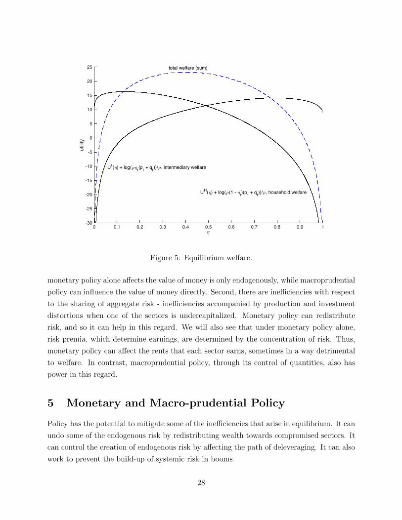
Welfare in equilibrium and preliminary thoughts on policy. Figure 5 shows

welfare for parameter values we described at the beginning of this section. For an economy

with K0 normalized to 1, Figure 5 shows the utility of a representative intermediary and

a representative household (normalizing wealth dispersion among households to 0). Recall

from Proposition 7 that welfare takes the form U I(η0) + log(ρn0)/ρ where n0 = η0(p0 + q0)

for intermediaries and UH(η0) + log(ρnH0 )/ρ where nH0 = (1− η0)(p0 + q0) for households.

The welfare of each agent type tends to increase in its wealth share, but only to a

certain point. At the extreme, one class of agents becomes so severely undercapitalized that

productive inefficiency makes everybody worse off - at those extremes redistribution towards

the undercapitalized sector would be Pareto improving. Total welfare is maximized near the

steady state of the system, but this property depends on the parameters we chose.

In the next section we discuss policy. Our primary focus is monetary policy, but we

also look at combinations of monetary and macroprudential policies. Before proceeding,

let us reiterate the inefficiencies present in our model, and discuss how policies may affect

these inefficiencies. First, as in the benchmark without intermediaries, there is the trade-

off between the value of money - the benefits it brings of helping hedge idiosyncratic risk

- and investment distortions that arise from the control of the value of money. Of course,

27

�0 0.1 0.2 0.3 0.4 0.5 0.6 0.7 0.8 0.9 1

utilit

y

-30

-25

-20

-15

-10

-5

0

5

10

15

20

25

UI(�) + log(��t(pt + qt))/�, intermediary welfare

UH(�) + log(�(1 - �t)(pt + qt))/�, household welfare

total welfare (sum)

Figure 5: Equilibrium welfare.

monetary policy alone affects the value of money is only endogenously, while macroprudential

policy can influence the value of money directly. Second, there are inefficiencies with respect

to the sharing of aggregate risk - inefficiencies accompanied by production and investment

distortions when one of the sectors is undercapitalized. Monetary policy can redistribute

risk, and so it can help in this regard. We will also see that under monetary policy alone,

risk premia, which determine earnings, are determined by the concentration of risk. Thus,

monetary policy can affect the rents that each sector earns, sometimes in a way detrimental

to welfare. In contrast, macroprudential policy, through its control of quantities, also has

power in this regard.

5 Monetary and Macro-prudential Policy

Policy has the potential to mitigate some of the inefficiencies that arise in equilibrium. It can

undo some of the endogenous risk by redistributing wealth towards compromised sectors. It

can control the creation of endogenous risk by affecting the path of deleveraging. It can also

work to prevent the build-up of systemic risk in booms.

28

Policies affect the equilibrium in a number of ways, and can have unintended conse-

quences. Interesting questions include: What is the effect on equilibrium leverage? Does

policy create moral hazard? Does policy lead to inflated asset prices in booms? What hap-

pens to endogenous risk? How does the policy affect the frequency of crises, i.e. episodes

characterized by resource misallocation and loss of productivity?

We focus on several monetary policies in this section. These policies can be divided in

several categories. Traditional monetary policy sets the short-term interest rate. It affects

the yield curve through the expectation of future interest rates, as well as through the

expected path of the economy, accounting for the supply and demand of credit, and risk

premia. When the zero lower bound for the short-term policy rate becomes a constraint,

forward guidance is an additional policy tool employed in practice. The use of this tool

depends on central bank’s credibility, as it ties the central bank’s hands in the future and

leaves it less room for discretion. In this paper we assume that the central bank can perfectly

commit to contingent future monetary policy and hence the interest rate policy incorporates

some state-contingent forward guidance.

Several non-conventional policies have also been employed. The central bank can directly

purchases assets to support prices or affect the shape of the yield curve. The central bank can

lend to financial institutions, and choose acceptable collateral as well as margin requirements

and interest rates. Some of these programs work by transferring tail risk to the central bank,

as it suffers losses (and consequently redistributes them to other agents) in the event that

the value of collateral becomes insufficient and the counterparty defaults. Other policies

include direct equity infusions into troubled institutions. Monetary policy tools are closely

linked to macroprudential tools, which involve capital requirements and loan-to-value ratios.

The classic “helicopter drop of money” has in reality a strong fiscal component as money

is typically paid out via a tax rebate. Importantly, the helicopter drop also has redistribu-

tive effects. As the money supply expands, the nominal liability of financial intermediaries

and hence the household’s nominal savings are diluted. The redistributive effects are even

stronger if the additional money supply is not equally distributed among the population but

targeted to specific impaired (sub)sectors in the economy.

Instead of analyzing fiscal policy, we focus this paper on conventional and non-conventional

monetary policy. For example, a change in the short-term policy interest rate redistributes

wealth through the prices of nominal long-term assets. The redistributive effects of monetary

policy depend on who holds these assets.11 In turn, asset allocation depends on the antic-

11Brunnermeier and Sannikov (2012) discuss the redistributive effects in a setting in which several sectors’

29

ipation of future policy, as well as the demand for insurance. Specifically, we introduce a

perpetual long-term bond, and allow the monetary authority to both set the interest rate on

short-term money, and affect the composition of outstanding government liabilities (money

and long-term bonds) through open-market operations.

5.1 Introducing Interest Bearing Reserves/Outside Money

So far, outside money – which we can think of as reserves held by the intermediary sector

– did not pay any nominal interest rate, and the total supply of outside money was fixed.

From the basic Fisher equation,12

drMt = dit − dπt,

we see that the real rate (the return on money) drM simply corresponded to the negative of

inflation, dπt. Indeed, given the fixed supply of outside money, economic growth – growth

in Kt – led to deflation. Furthermore, whenever ηt declines, i.e. whenever the intermediary

sector has suffered losses and is constrained in its ability to take on risk, deflation becomes

even more pronounced.

In this section, we will allow for more general monetary policies. LetMt denote the total

supply of outside money. In general, dMt/Mt can follow any stochastic process which may

include possible jumps.

For most part of this paper, we assume that the central bank “prints” new outside

money simply to pay the interest on existing stock of outside money, i.e. dMt/Mt = dit.

This assumes that newly printed money is distributed to existing holders of outside money

(reserves). Note that nowadays most advance-economy central banks, including the U.S.

Federal Reserve, pay (nominal) interest on reserves. Since intermediary sector is competitive

in our model, a higher interest rate on outside money is passed on to inside money holders

as well. Outside money and inside money remain to have the same return and risk profile.

Price flexibility ensures that any monetary policy rule leaves ηt unaffected in our simple

setting. However, monetary policy evidently does have an effect on inflation. The Fisher

balance sheets can be impaired. Forward guidance not to increase the policy interest rate in the near futurehas different implications than a further interest rate cut, since the former narrows the term spread whilethe latter widens it.

12We write dπ instead of π to capture the possibility that the price level might jump. In most of the paperwe do not, in fact, allow for such jumps; the analysis of money supply rules in this section is an exception.

30

equation, reveals that inflation has two components: a purely monetary component related

to the money supply growth rule, and a real component that reflects the various amplification

spirals discussed in the previous section (which one could coin “real inflation”).

dπt = dit − drMt =dMt

Mt

− drMt =dMt

Mt

− d(ptKt)

ptKt

We summarize our results as follows.

Proposition 8. (Super-Neutrality of Money) Suppose that outside money follows the growth

rule, then the analysis of Section 4 goes through unaffected, with the single difference that

inflation now is

dπt =dMt

Mt

− d(ptKt)

ptKt

.

In particular, the law of motion and stationary distribution of ηt are unaffected.

We see that inflation has two components:

Our super-neutrality result is relevant for the old money view vs. credit view debate.

The money view, which can be traced back to Friedman and Schwartz’s monetarism and

even to the work of Irving Fisher on the Great Depression, posits that replacing in times

of crisis the “missing inside money” with additional outside money suffices to stabilize the

economy. This result fails to hold in our model – distribution-neutral money printing re-

duces disinflation, but does nothing to change real allocations. Thus, in our model, simple

inflation targeting does not reduce any amplification spirals and so does not help stabilize

the economy. Also, within the set of money supply rules that we consider, the Friedman rule

has no special place. The Friedman rule recommends for settings in which money pays no

interest a deflation rate that equalizes the real return of money with the real risk-free rate.

In our setting with interest bearing reserves and flexible prices, the Friedman rule – just like

all the other money supply rules – has no real effects, and so certainly is not strictly optimal

within the restricted set of money supply growth rules.

The credit view, pushed primarily by Tobin, stresses the importance of restoring bank

lending, and so is more concerned with the asset side of intermediaries’ balance sheets. Mon-

etary policy that redistributes towards intermediaries can switch off amplification spirals and

so improve the risk-bearing capacity of the financial sector. More generally, a monetary pol-

icy that recapitalizes balance sheet-impaired sectors can help stabilize the economy and, in

31

fact, may well be welfare-improving. In practice, monetary authorities do not provide out-

right redistribution between sectors – this is the domain of fiscal policy. However, as we will

illustrate in the section, both conventional and unconventional monetary policy measures

(ranging from simple nominal interest rate movements to central bank purchases of long-

term assets) may well indirectly (“sneakily”) re-distribute wealth between sectors. In the

monetary policy can provide the desired stabilization – all in spite of complete price flexibility.

A couple of final remarks are in order. First, we need to emphasize that our negative

results regarding the money view apply to money supply policies specifically designed to

keep ηt fixed. As soon as the newly printed money is distributed in a way somehow different

from the existing money holdings or not passed on to inside money holders, wealth shares

are impacted, and so we have real implications. For example, the classic “helicopter drop

of money” would have redistributive effects. As the money supply expands, the nominal

liability of financial intermediaries and hence the household’s nominal savings are diluted.

The redistributive effects are even stronger if the additional money supply is not equally

distributed among the population but targeted to specific impaired (sub)sectors in the econ-

omy. Thus, as soon as the newly printed money is distributed in a way somehow different

from the existing (outside and inside) money holdings, wealth shares are impacted, and so

we have real implications. We conclude that, for the money view to be revived in our model,

monetary intervention needs to take on an explicit redistributional dimension. This calls for

a richer modeling environment, which we will provide in the next section. Second, note that

our results are derived under the assumption of complete price flexibility. Our emphasis on

the credit view comes out naturally in a model with financial frictions but no price-setting

frictions. Of course, matters will look different in a model with price rigidity but no financial

frictions.

5.2 Introducing Nominal Long-term Bonds

Money and Long-Term Bonds. We now extend our baseline model to allow for a re-

alistic monetary policy with distributional – and so real – effects. The extended model

differs from the baseline model along two dimensions. First, as in our earlier discussion

of non-redistributional monetary policy, we allow money/reserves to pay a floating rate of

interest it, set freely by the central bank. Second, we introduce perpetual bonds that can

be issued by the government. This nominal bond pays interest at a fixed rate iB in money.

32

The monetary authority sets the total quantity outstanding of (nominal) perpetual bonds

Bt (quantitative easing, or QE in short). We restrict both policies to be revenue neutral –

the monetary authority pays interest and/or performs QE operations so that there are no

fiscal implications. In other words, the central bank does not alter its seignorage income

when changing its monetary policy.

Interest rate policy. First consider interest rate policy – the conventional monetary

policy. To fix ideas, let us trace the implications of an interest rate cut. Cutting the short-

term rate on money means that the central bank pays less money on the existing outside

money stock. This then lowers the growth rate of outside money dMt/Mt. Since banking

is competitive, this decrease in interest paid on outside money is passed through one-to-one

to interest payment on inside money. The direct effect of this interest rate cut is, just as we

have seen above in the model without a long-term government bond, disinflationary. Now,

however, there is an important indirect effect: Since the long-term bond continues to pay

interest at a fixed nominal rate iB, the price of the nominal bond relative to nominal money

increases. Furthermore, as we will see later, under standard monetary policy specifications

the perpetual bonds are held exclusively by the intermediaries. In short, intermediaries are

long perpetual bonds and short inside money. As the price of bonds relative to the price

of money rises, the intermediaries’ wealth share η increases. For a low η the liquidity and

disinflationary spirals are thus mitigated, so that overall the second indirect effect of the rate

cut is, in fact, inflationary. Algebraically, this can be seen in equation (5.1): dMt/Mt falls

– the direct effect – but d(−ptKt)/ptKt rises – the indirect effect. Overall, for the indirect

effect to dominate, the response of bond prices needs to be sufficiently strong. As we will

see later, a sufficient statistic for this response is the elasticity B′(η)B/η

, where B denotes the

nominal price of a single long-term bond in terms of money. As long as the central bank

has perfect commitment power - its forward guidance is credible, this elasticity can be made

arbitrarily large. For example, if the central bank were to commit to set the short-term

interest rate to zero forever (say when η drops below a certain threshold) then the relative

price of the bond Bt tends to infinity. Thus, around this threshold level the elasticity is very

high.

These results relate to the recent debate on the interpretation of the Fisher equation

and, more broadly, the relationship between nominal interest rates and inflation. Do high

interest rates beget high or low inflation (and vice-versa for low interest rates)? In the

33

model without long-term bonds – like in all models in which money is superneutral –, for

simple money supply growth rules, high interest rates beget high inflation, consistent with

the recent, Fisher equation-based re-interpretation on the inflation/interest rate linkages.

Conversely, as soon as interest rate movements are associated with stabilizing changes in

wealth shares, the traditional short-run monetary policy view is restored. Interest rate cuts

that re-distribute towards the balance sheet-impaired financial sector stabilize the economy

and so tend to push up inflation.

Asset purchase programs/Quantitative Easing (QE). The implications of quanti-

tative easing for the evolution of total outside money are more subtle. Instantaneously, QE is

financed through money issuance, so central bank purchases of long-term bonds go together

with increases in (short-term) outside money. But since the public is then left with fewer

long-term bonds, total nominal interest payments over time are lower than before, pushing

down the rate of increase of outside money dMt/Mt. At the same time, QE means that the

price of the remaining long-term bonds relative to money rises, so again intermediaries are

recapitalized. Thus the indirect inflationary effect of interest rate cuts is also present after

expansionary asset purchase programs.13 At first glance, one might think that households

could simply undo the central bank’s QE by adjusting their portfolio. Indeed, Wallace (1981)

derived this Modigliani-Miller type result: Under the assumption that all investors can in

theory purchase and short-sell arbitrary quantities of all assets at the given market prices,

QE has no real effects. In contrast, in our model, and consistent with reality, households

cannot issue long-term bonds, and so Wallace neutrality breaks down. Again, the strength

of these effects can be summarized via the sufficient statistic B′(η)B/η

.

Since the elasticity B′(η)B/η

features prominently in the analysis of both policies, we will from

now on merge the presentation of the two policy examples and, more abstractly, consider

the real price of bonds as a policy instrument.

Formal Analysis. For our formal analysis we denote by ptKt the real value of all

13In reality, central bank asset purchases have not been restricted to long-term government bonds, butalso included risky private sector assets. In our model, this could mean risky claims held by the intermediarysector. Whether or not such purchases would help stimulate our economy depends crucially on whether thecentral bank can, just like intermediaries, provide a “diversification service”. If the central bank is as badas households in diversifying away idiosyncratic risk, then the asset purchases are ineffective. In contrast, ifthe central bank is as good as the intermediary sector, then it should just take over. In reality, the truth islikely to lie somewhere in between. We leave this extension for further research.

34

outstanding nominal assets: outside money and perpetual bonds. We denote Mt the real

value of (short-term) outside money and let btKt be the real value of all outstanding perpetual

bonds. btKt is affected by total supply of outstanding number of bonds Bt and real value of

the bonds. Each individual bond’s nominal value is endogenous in equilibrium and denoted

by Bt. We postulate that Bt follows the following endogenous equilibrium process:

dBt

Bt

= µBt dt+ (σBt )T dZt. (5.1)

The real value of the perpetual bond is MtBt.

Note that the central bank chooses the nominal interest rate it paid on short-term outside

money and the number of outstanding perpetual nominal bonds Bt = (btKt)/(MtBt). To

simplify the analysis, we do not treat (it,Bt) as the policy tool pair of the central bank,

but instead conjecture that it can equivalently control bt and so consider the (dual) policy

instrument pair (it, bt). In the analysis, it then simply remains to take into account the fact

that Bt still evolves endogenously.

Returns. The expressions for the return on capital from Section 2 do not change, but

money earns the return that depends on policy. If an agent holds all nominal assets in the

economy - bonds and outside money - the return is

(Φ(ι)− δ + µpt + (σpt )

TσKt)dt+ (σKt + σpt )

T dZt.

This is the return on a portfolio with weights bt/pt on bonds and 1 − bt/pt on money. To

isolate the returns on money and bonds, consider a strategy that buys bonds to earn drBt

by borrowing money, paying drMt . We can find the payoff of this strategy by focusing on the

value of bonds in money. Using Ito’s lemma,

drBt − drMt =

(1

Bt

− it + µBt + (σBt )TσMt

)dt+ (σBt )T dZt,

where σMt is the risk of money, which satisfies

σKt + σpt = σMt +btptσBt ⇒ σMt = σKt + σpt −

btptσBt . (5.2)

35

Thus, money earns the return of

drMt =(Φ(ι)− δ + µpt + (σpt )

TσKt)dt− bt

pt

(1

Bt

− it + µBt + (σBt )TσMt

)dt+ σMt dZt. (5.3)

Equilibrium Conditions. For expositional purposes, we focus on policies that set the

short-term interest rate it and the value of bonds bt as functions of the state variable ηt.

Then the price of bonds Bt will also be a function of ηt. Consider for concreteness policies

that lead to a decreasing function B(η), which follows from policies that cut the short-term

interest rate when ηt is low, making bonds appreciate. Such a policy is designed to help

intermediaries transfer some of the aggregate risk to households - by borrowing money and

buying long-term bonds, intermediaries get a natural hedge that gives them insurance in

the event that ηt drops and the entire intermediary sector suffers losses. The appreciation

in bonds can offset partially other risks that the intermediaries face, including endogenous

risks driven by amplification. In the equations below, we assume that intermediaries hold

all long-term bonds as a hedge, and later verify that this is indeed the case.

To adjust for policy, we have to take into account that the risk of money, entering

the expressions for νt, νat , σ

Nat and σNbt is now given by (5.2). Furthermore, the risk of

intermediaries net worth, which has to be adjusted for the bonds they hold, now takes the

form

σNt = σMt + xtνt + xBt σBt , where xBt =

ϑtηt

btpt

is the portfolio weight on bonds.

The asset pricing conditions for capital invested in technologies a and b take the same

form (2.11) and (2.10), but with the adjusted values of νt, νat , σ

Nt , σ

Nat and σNbt .

In addition, we have a new pricing condition for bonds,

1

Bt

− it + µBt + (σBt )TσMt = (σBt )TσNt ≤ (σBt )T (σMt + xat νt)︸ ︷︷ ︸σNat

, (σBt )T (σMt + xbtνbt )︸ ︷︷ ︸

σNbt

.

Note that 1Bt− it is the nominal term spread. If the long-term bond is risk-free, i.e.

σB = 0, then the term spread has to equal to the depreciation rate of the bond.

The law of motion of ηt, likewise, has to be adjusted for the risk that the intermediaries

are now exposed to.

36

Proposition 9. The equilibrium law of motion of ηt is given by

dηtηt

= (1− ηt)(|xtνbt + xBt σ

Bt |2 − (xat )

2(|νat |2 + (σa)2))dt+ (5.4)

(xtν

bt + σϑt + (1− ηt)xBt σBt

)T (dZt +

(σϑt − ηtxBt σBt

)dt).

Proof. See Appendix.

Mitigated Liquidity and Disinflationary Spiral. The effect of monetary policy on

the asset-pricing conditions as well as the law of motion of ηt enters exclusively through the

term (bt/pt)σBt . If monetary policy sets the short-term interest rate it as well as the level of

bt as functions of ηt, then the risk of the bond price σBt is collinear with σa1a − σKt , σηt and

σϑt . Thus, monetary policy can be used implement more efficient sharing of aggregate risk,

e.g. undo endogenous risk.

For example, when intermediaries borrow money to invest in equity of projects b, the

incremental risk they take is given by

νt =

(1− ϑ′(η)

ϑ(η)(1− ϑ(η))+b(η)

p(η)

B′(η)

B(η)

)(σa1a − σKt

). (5.5)

Thealternative candidate is

νt = σb1b − σKt −1

1− ϑ(ηt)

ϑ′(ηt)

ϑ(ηt)/ηtσηt +

b(ηt)

p(ηt)

B′(ηt)

B(ηt)/ηtσηt

In this equation ϑ′(η)ϑ(η)(1−ϑ(η))

reflects the amplification of aggregate risk σa1a−σKt through

the changing prices pt and qt, while b(η)p(η)

B′(η)B(η)

reflects the mitigation of this risk through mon-

etary policy. In the following section, we study the risk transfer effects of monetary policy

by focusing on the mitigating term. The one-dimensional function b(η)p(η)

B′(η)B(η)

of η summarizes

the effects of two policy tools it and bt, with which any such function can be implemented

in multiple ways.

37

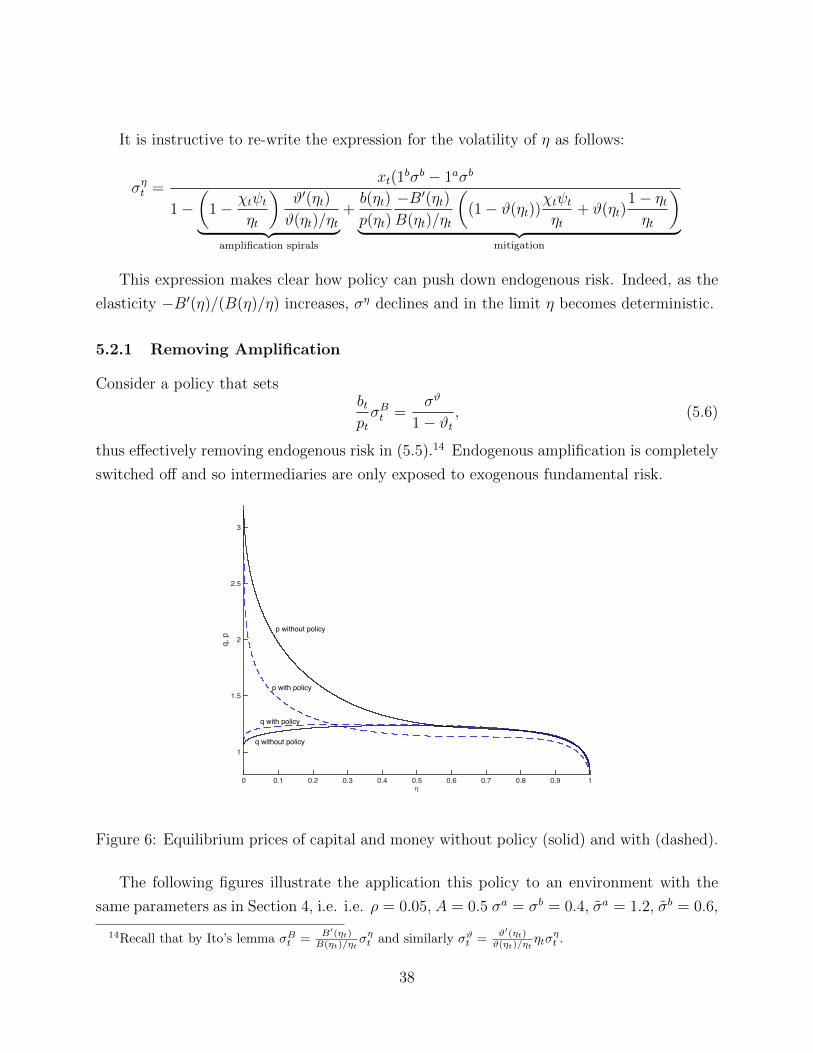
It is instructive to re-write the expression for the volatility of η as follows:

σηt =xt(1

bσb − 1aσb

1−(

1− χtψtηt

)ϑ′(ηt)

ϑ(ηt)/ηt︸ ︷︷ ︸amplification spirals

+b(ηt)

p(ηt)

−B′(ηt)B(ηt)/ηt

((1− ϑ(ηt))

χtψtηt

+ ϑ(ηt)1− ηtηt

)︸ ︷︷ ︸

mitigation

This expression makes clear how policy can push down endogenous risk. Indeed, as the

elasticity −B′(η)/(B(η)/η) increases, ση declines and in the limit η becomes deterministic.

5.2.1 Removing Amplification

Consider a policy that setsbtptσBt =

σϑ

1− ϑt, (5.6)

thus effectively removing endogenous risk in (5.5).14 Endogenous amplification is completely

switched off and so intermediaries are only exposed to exogenous fundamental risk.

�0 0.1 0.2 0.3 0.4 0.5 0.6 0.7 0.8 0.9 1

q, p

1

1.5

2

2.5

3

p without policy

p with policy

q with policy

q without policy

Figure 6: Equilibrium prices of capital and money without policy (solid) and with (dashed).

The following figures illustrate the application this policy to an environment with the

same parameters as in Section 4, i.e. i.e. ρ = 0.05, A = 0.5 σa = σb = 0.4, σa = 1.2, σb = 0.6,

14Recall that by Ito’s lemma σBt = B′(ηt)B(ηt)/ηt

σηt and similarly σϑt = ϑ′(ηt)ϑ(ηt)/ηt

ηtσηt .

38

s = 0.8, Φ(ι) = log(κι+ 1)/κ with κ = 2, and χ = 0.001. Figure 6 shows the effect of policy

on prices. The price of money falls since the intermediary sector creates more inside money:

it does not need to absorb as much aggregate risk to do that. As a consequence, the price

of capital rises - there is more demand for capital from the sector producing good a, and as

Figure 7, capital is shifted to sector a.

�0 0.1 0.2 0.3 0.4 0.5 0.6 0.7 0.8 0.9 1

capi

tal a

lloca

tion

0

0.1

0.2

0.3

0.4

0.5

0.6

0.7

0.8

0.9

1

�t (1 - � t), with policy

�t (1 - � t), without policy

�t � t , without policy

�t � t , with policy

1 - �t , with policy

1 - �t , without policy

Figure 7: Equilibrium allocations without policy (solid) and with (dashed).

Finally 8 shows the drift and volatility of η with and without policy. With policy, the

intermediary net worth is lower at the steady state. Consequently, their leverage is higher.

Ultimately, monetary policy transfers risk, but it controls quantities only indirectly – the

allocation of capital, the value of money relative to capital, and earnings rates of sectors a

and b as well as intermediaries are endogenously determined by the allocation of risk.

5.2.2 Economy with Perfect Sharing of Aggregate Risk

Recall Equation (??),

σηt =xt(σ

b1b − σKt )

1−(ψt(1− χt)− ηt

ηt

)−ϑ′(ηt)ϑ/ηt︸ ︷︷ ︸

amplification spirals

+

(ψt(1− χt)− ηt

ηt+ϑtηt

(1− ψt)btpt

−B′(ηt)B/η

)︸ ︷︷ ︸

mitigation→∞

39

�0 0.1 0.2 0.3 0.4 0.5 0.6 0.7 0.8 0.9 1

� ��, |� ��|

-0.04

-0.02

0

0.02

0.04

0.06

0.08

� t� �, without policy

� t� �, with policy

|�t� �|, with policy

|�t� �|, without policy

Figure 8: Drift and volatility of η without policy (solid) and with (dashed).

Now let the mitigation term in the denominator go to infinity, so that ultimately σηt → 0.

We are thus in an economy where aggregate risk is shared perfectly. Indeed, this is exactly

the outcome we would see if intermediaries and households could trade contracts based on

systemic risk, i.e. risk of the form

(σa1a − σb1b)T dZt

With all agents sharing aggregate risk perfectly, the aggregate risk exposure of both house-

holds and intermediaries is proportional to σKt , and ηt, pt and qt have no volatility. Fur-

thermore, perfect sharing of aggregate risk implies that households who produce good a will

retain the minimal allowed fraction of equity, χ.

The following proposition characterizes the function ϑ(η) through a first-order differential

equation, together with ψt, household leverage xat and xbt , price qt and the dynamics of η.

Proposition 10. The function ϑ(η) satisfies the first-order differential equation

µϑt =ϑ′(η)

ϑ(η)ηµηt , (5.7)

40

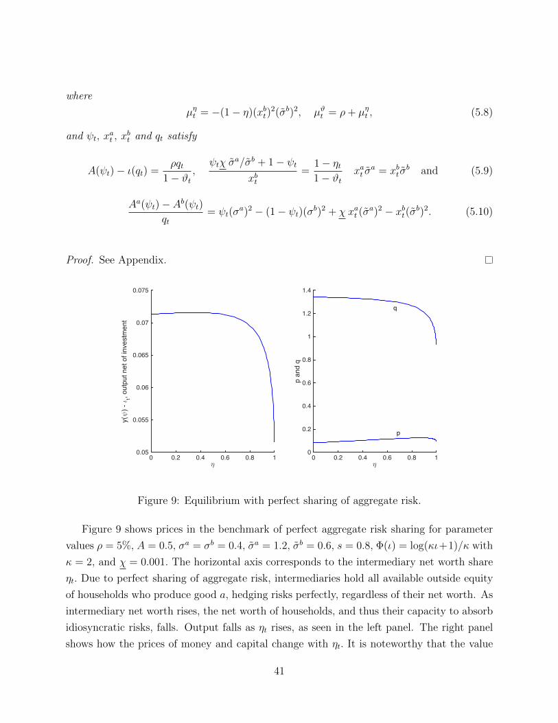
where

µηt = −(1− η)(xbt)2(σb)2, µϑt = ρ+ µηt , (5.8)

and ψt, xat , x

bt and qt satisfy

A(ψt)− ι(qt) =ρqt

1− ϑt,

ψtχ σa/σb + 1− ψtxbt

=1− ηt1− ϑt

xat σa = xbt σ

b and (5.9)

Aa(ψt)− Ab(ψt)qt

= ψt(σa)2 − (1− ψt)(σb)2 + χ xat (σ

a)2 − xbt(σb)2. (5.10)

Proof. See Appendix.

�0 0.2 0.4 0.6 0.8 1

y(�

) - � t, o

utpu

t net

of i

nves

tmen

t

0.05

0.055

0.06

0.065

0.07

0.075

�0 0.2 0.4 0.6 0.8 1

p an

d q

0

0.2

0.4

0.6

0.8

1

1.2

1.4

q

p

Figure 9: Equilibrium with perfect sharing of aggregate risk.

Figure 9 shows prices in the benchmark of perfect aggregate risk sharing for parameter

values ρ = 5%, A = 0.5, σa = σb = 0.4, σa = 1.2, σb = 0.6, s = 0.8, Φ(ι) = log(κι+1)/κ with

κ = 2, and χ = 0.001. The horizontal axis corresponds to the intermediary net worth share

ηt. Due to perfect sharing of aggregate risk, intermediaries hold all available outside equity

of households who produce good a, hedging risks perfectly, regardless of their net worth. As

intermediary net worth rises, the net worth of households, and thus their capacity to absorb

idiosyncratic risks, falls. Output falls as ηt rises, as seen in the left panel. The right panel

shows how the prices of money and capital change with ηt. It is noteworthy that the value

41

of money is very low relative to both the money regime and the full equilibrium that we

describe in the next section. The value of money ϑt relative to total wealth rises. The drift

of ηt is always negative, as shown on the right panel and seen from (5.8).

In contrast, without intermediaries (3.3) implies that the prices of capital and money

would be q = 1.0655 and p = 3.79 (see Lemma ? in the Appendix). The value of money

is significantly higher under the benchmark without intermediaries who provide insurance

against almost all of idiosyncratic risk of technology a. This fact creates the possibility of a

significant deflationary spiral in our full model, in which the intermediaries have to absorb

some of aggregate risk, and their capacity to function depends on having sufficient net worth.

42

5.3 Welfare

We have to adjust the equations from Section 4.2 somewhat since the baseline return on

money is given by the generalized formula (5.3).

Proposition 11. The welfare of an agent with wealth nt who can invest only in money is

given by ω(η) + log(nt/pt)/ρ, where ω(η) satisfies

ρω(ηt) = log(ρpt) + µηt ηω′(η) +

|σηt η|2

2ω′′(η)+

Φ(ι)− δ − ρ− (σKt )2 − btptσBt (xtνt + ϑt

ηtbtptσBt )T + ( bt

ptσBt )2/2

ρ. (5.11)

The welfare of an intermediary with net worth nt is h(ηt) + ω(ηt) + log(nt/pt)/ρ, where

ρh(η) =x2t |νt|2

2ρ+ h′(η)µηt η +

h′′(η)η2σηt (σηt )T

2. (5.12)

The welfare of a household is hJ(ηt)+ω(ηt)+ log(nt/pt)/ρ, where hJ satisfies equation (D.2)

with the term x2t |νt|2 replaced by (xJt )2|νJt |2.

Proof. From the bond-pricing condition, the return on money (5.3) can be written as

(Φ(ι)− δ + µpt + σpt (σ

Kt )T

)dt− bt

ptσBt (σNt ) dt+ (σKt + σpt −

btptσBt ) dZt.

Conjecturing the form ω(ηt) + log(nt/pt)/ρ for the value function of someone who invests

only in money, the HJB equation is

ρω(ηt) + log(nt/pt) = log(ρnt) + µηt ηω′(η) +

|σηt η|2

2ω′′(η)+

Φ(ι)− δ − ρ+ µpt + σpt (σKt )T − bt

ptσBt (σNt )T

ρ−

(σKt + σpt − btptσBt )2

2ρ− µpt

ρ+

(σpt )2

2ρ.

Plugging in

σNt = σMt + xtνt +ϑtηt

btptσBt , σMt = σKt + σpt −

btptσBt ,

the equation for ω simplifies to (5.11). Furthermore, as in the proof of Proposition 13,

the welfare of any agent with richer investment opportunities has to be adjusted by the

incremental risk that the agent chooses to take. In particular, the welfare of an intermediary

43

with net worth nt is given by h(ηt)+ω(ηt)+log(nt/pt)/ρ, where h(η) satisfies (5.12). Likewise,

to get the welfare of households hJ(ηt) + ω(ηt) + log(nt/pt)/ρ, we have to replace the term

x2t |νt|2 with (xJt )2|νJt |2.

The relevant boundary conditions are the same as without policy, since the policy affects

equilibrium dynamics only in the interior of the state space [0, 1] and not on the boundaries.

5.4 Policies that undo Endogenous Risk.

The risk that intermediaries take on by buying more capital is captured by

νt =

(1− ϑ′(η)

ϑ(η)(1− ϑ(η))+btpt

B′(η)

B(η)

)ψJt

(σI

1I

I− σJ 1J

J

)︸ ︷︷ ︸

fundamental risk

=

(1 + αt) ψJt

(σI

1I

I− σJ 1J

J

)where the term −ϑ′(η)

ϑ(η)(1−ϑ(η))> 0 amplifies the risk that intermediaries face and bt

pt

B′(η)B(η)

can

mitigate it.

Likewise, the risk that households take on by buying capital is

νjt = (1jσJ − σK) +

(− ϑ′(η)

ϑ(η)(1− ϑ(η))+btpt

B′(η)

B(η)

)ψJt

(σI

1I

I− σJ 1J

J

)︸ ︷︷ ︸

fundamental risk

,

which consists of idiosyncratic risk and average J-household risk

νJt = −(1−ψJ)

(σI

1I

I− σJ 1J

J

)+αtψ

Jt

(σI

1I

I− σJ 1J

J

)= (αtψ

Jt −(1−ψJ))

(σI

1I

I− σJ 1J

J

)It looks like αt > 0 in the absence of monetary policy, and monetary policy can reduce

αt. Effectively, this action shifts risk between technologies I and J - a reduction in α shifts

risk in favor of I. Policy affects the world portfolio, and this (1) the total output/productive

efficiency, (2) the amount of idiosyncratic risk exposure.

The agents’ risk exposures are given by

σKt + σqt − αtψJt(σI

1I

I− σJ 1J

J

)︸ ︷︷ ︸

σMt

+xJt (αtψJt − (1− ψJ))

(σI

1I

I− σJ 1J

J

)+ xJt dε

jt .

44

by which fundamental risk is amplified. We observe that amplification is significant,

particularly below the steady state when intermediaries are undercapitalized.

In this section we consider the effect of policy that completely removes endogenous risk

by setting instruments bt and rt in such a way that

σϑ

1− ϑ= σpt − σ

qt =

btptσBt . (5.13)

This can be done in multiple ways, since we have the flexibility to choose two functions of η

to match a single condition (5.13). If (5.13) holds, then

νt = σI1I

I− σKt νit = σI1i − σKt and νjt = σI1j − σKt

i.e. the incremental risk that any agent faces by adding capital to his/her portfolio is only

fundamental and not endogenous. In this section we show that the equilibrium dynamics

that results under any such policy can be characterized in terms of a single second-order

differential equation for the function ϑ(η).

First, the law of motion of ηt can be found from (5.4). Given (5.13), this reduces to

dηtηt

= (1− ηt)

(∣∣∣∣xtνt +ϑtηt

σϑ

1− ϑ

∣∣∣∣2 dt− |xJt νJt |2)dt+

(1− ηtηt

ϑtσϑ

1− ϑt+ xtνt

) (dZt −

ϑσϑ

1− ϑdt

). (5.14)

Thus,

σηt = xt

(σI

1I

I− σKt

)+

1− ηt1− ϑt

ϑ′(η)ση ⇒ σηt =xt

(σI 1I

I− σKt

)1− 1−ηt

1−ϑt ϑ′(η)

,

where the denominator has dampening effect as long as ϑ′(η) < 0, since it reduces the risk

of η. Second, the function ϑ(η) it self can be found via the following procedure.

Procedure. The function ϑ(η) that results under any policy that removes endogenous

risk according to (5.13) has to satisfy the following second-order differential equation. First,

45

given η and (ϑ(η), ϑ′(η)) the allocation of capital (ψt, ψJt ) must satisfy the conditions

xt =ψt(1− ϑ(η))

ηt, σηt =

xt

(σI 1I

I− σKt

)1− 1−ηt

1−ϑt ϑ′(η)

, σϑt =ϑ′(η)

ϑ(η)σηt η, Y − ι(q) =

ρq

1− ϑ(η),

xt|νt|2+νtϑtηt

(σϑ)T

1− ϑ= xIt |νIt |2,

(P it − P

jt )a

qt= (σI1i−σJ1j)(σKt )T +xIt |νIt |2−xJt |νJt |2. (5.15)

η +ψJ(1− ϑ(η))

xJt︸ ︷︷ ︸ηJ

+(1− ψJ − ψ)(1− ϑ(η))

xIt︸ ︷︷ ︸ηI

= 1 and (xIt )2|νIt |2 ≤ (xJt )2|νJt |2,

with equality of ψ + ψJ < 1. Then,

P It a− ιq

+σϑ

1− ϑσηt = νt

(σηt +

ϑtσϑ

1− ϑt+ σKt

)T+

µϑ

1− ϑ(5.16)

and ϑ′′(η) =µϑϑ(η)− ϑ′(η)µηt η

η2σηt (σηt )T/2,

where the volatility of η, µηt , is taken from (5.14).

Proof. We only need to justify the expressions that appear in the above procedure for the

first time. Note that

σNt = σKt + σpt −btptσBt︸ ︷︷ ︸

σMt =σKt +σqt

+xt

(σI

1I

I− σKt

)+ϑtηt

σϑ

1− ϑ,

Subtracting the capital pricing conditions for intermediaries and households who hold capital

types i = 1, . . . I, we obtain

xt|νt|2 + νtϑtηt

(σϑ)T

1− ϑ= xIt |νIt |2,

since νt(σMt )T = νit(σ

Mt )T . Furthermore, the capital pricing conditions of intermediaries and

46

households who hold capital types j = I + 1, . . . I + J, we find

(P it − P

jt )a

qt+ (σIt 1

i − σjt1j)(σqt )T = xIt |νIt |2 − xJt |νJt |2 + (σIt 1

i − σJt 1j)(σKt + σqt )T ,

which simplifies to the second equation in (A.1).

Finally, from the capital and bond pricing conditions for intermediaries, we obtain

E[drIt − drMt ]

dt=P It a− ιq

+ µqt − µpt + σqt

(σI

1I

I

)T− σpt (σKt )T +

σϑ

1− ϑ(σNt )T = νtσ

Nt

Since

σNt = σηt +ϑtσ

ϑ

1− ϑt+ σMt and

µpt − µqt =

σϑ

1− ϑσp − (σϑ)2

1− ϑ+

µϑ

1− ϑ, σpt − σ

qt =

σϑt1− ϑ

,

we haveP It a− ιq

+σϑ

1− ϑσηt = νt

(σηt +

ϑtσϑ

1− ϑt+ σKt

)T+

µϑ

1− ϑ,

as required.

We can verify analytically that for this policy, only intermediaries choose to hold long-

term bonds. The following proposition states this fact.

Proposition 12. Under the policy that removes endogenous risk, if ϑ′(η) < 0 for all η ∈(0, 1), then only intermediaries want to hold bonds at all points of the state space. That

is, the required risk premium for bond holdings is lower for intermediaries than any other

agents, i.e.

σBt (σNt )T ≤ σBt (σMt + xJt νJt )T , σBt (σMt + xItν

It )T , (5.17)

where σNt = σMt + xtνt + ϑtηt

σϑ

1−ϑt .

Proof. First, note that

νt = ψJ(σI

1I

I− σJt

1J

J

), |νt|2 = νIt νt = (ψJt )2

((σI)2

I− (σJ)2

J

)

and νt(νJt )T = −(1− ψJ)ψJ

((σI)2

I− (σJ)2

J

).

47

Furthermore,

σBt =ptbt

σϑt1− ϑt

=ptbt

ϑ′(η)

ϑt(1− ϑt)ηtxt

1− 1−ηt1−ϑt ϑ

′(η)︸ ︷︷ ︸A<0

νt.

Thus, (5.17) is equivalent to

νt

(xtνt +

ϑtηt

σϑ

1− ϑt

)T≥ xJt νt(ν

Jt )T , xItνt(ν

It )T .

The first inequality holds since xJt νt(νJt )T < 0 and

xtνt +ϑtηt

σϑ

1− ϑt= xtνt +

ϑ′(η)

1− ϑtxt

1− 1−ηt1−ϑt ϑ

′(η)︸ ︷︷ ︸σηt

νt = xt1 + ηt

1−ϑt ϑ′(η)

1− 1−ηt1−ϑt ϑ

′(η)︸ ︷︷ ︸>0

νt,

so νt

(xtνt + ϑt

ηtσϑ

1−ϑt

)T> 0. The second inequality holds since

νt

(xtνt +

ϑtηt

σϑ

1− ϑt

)= xIt |νIt |2,

and |νIt |2 > |νt|2, specifically,

|νIt |2 = |νt|2 + (σI)2 I − 1

I.

Who holds the bonds... note also that the intermediaries’ greater willingness to hold

bonds depends on

σϑ(xν + ϑ/ησϑ/(1− ϑ)) < σϑxJνJ ,

i.e. the intermediaries’ required risk premium for holding bonds is lower...

Implementation. The condition (5.13) requires

d

dηlog ϑ(η) =

bt(1− ϑt)pt

d

dηlogB(η).

This makes it pretty easy to solve for logB(η). Since B is steeper than ϑ, the policy may

need to buy access bonds when η is low (quantitative easing) and reverse the policy when η

48

is high.

compare...

P It a− ιqt

=

(νt −

σϑt1− ϑt

)(σηt + σKt )T + σKt (σϑt )T +

(σI

1I

I

)ϑt(σ

ϑ)T

1− ϑt+

µϑ

1− ϑ

µϑ

1− ϑ=P It a− ιq

− (σηt + σKt )νTt − σKt (σϑt )T − ϑσϑt1− ϑ

(σI

1I

I

)TCombining (??) and (??), we obtain xt|νt|2 = xIt |νIt |2 since νt(σ

Kt + σpt ) = νIt (σKt + σpt ).

Subtracting (??) and (??), we obtain

(P It − P J

t )a

q+ (σI1i − σJ1j)(σqt )

T = xIt |νIt |2 − xJt |νJt |2 + (σI1i − σJ1j)(σKt + σpt )T ,

which implies the second equation in (??) since σpt − σqt = σϑt /(1 − ϑ). Finally, (??) is

expanded to

P It a− ιq

+ µqt − µpt + σqt

(σI

1I

I

)T− σpt (σKt )T = xtνtν

Tt + νt(σ

Kt + σpt )

T (5.18)

Since

µpt − µqt =

σϑ

1− ϑσp − (σϑ)2

1− ϑ+

µϑ

1− ϑ, σpt − σ

qt =

σϑt1− ϑ

,

and σηt = xtνt + σϑt , we have (5.18) can be transformed to

P It a− ιq

− µϑ

1− ϑ= (σηt + σKt )νTt + σϑt (σKt )T + σI

1I

I

ϑσϑt1− ϑ

,

which confirms (A.2).

We have

(P it − P

jt )a

qt+ σqt (σ

i1i − σj1j) = νt(σMt + xtνt +

ϑtηt

σϑ

1− ϑ)T − νJt (σMt + xJt ν

Jt )T .

(P it − P

jt )a

qt= (σi1i − σj1j)σKt + xt|νt|2 + νt

ϑtηt

(σϑ)T

1− ϑ− xJt |νJt |2.

49

The pricing conditions for capital and money on the intermediaries balance sheets are

Et[drIt − drMt ]

dt= νt(σ

Nt )T and

1

Bt

− rt + µBt + σBt (σMt )T = σBt (σNt )T .

Likewise, the households optimal allocations to capital xIt and xJt must satisfy

Et[drIt − drMt ]

dt= νIt (σMt + xItν

It )T and

Et[drJt − drMt ]

dt= νJt (σMt + xJt ν

Jt )T .

We must also verify that

1

Bt

− rt + µBt + σBt (σMt )T ≤ σBt (σMt + xItνIt )T , σBt (σMt + xJt ν

Jt )T

drIt =P It a− ιq

dt+

(Φ(ι)− δ + µqt + σqt

(σI

1I

I

)T)dt+

(σqt + σI

1I

I

)dZt,

drMt =(Φ(ι)− δ + µpt + σpt (σ

Kt )T

)dt− σϑ

1− ϑ(σNt )T dt+ σMt dZt.

Ok

P It a− ιq

+ µqt − µpt + σqt

(σI

1I

I

)T− σpt (σKt )T +

σϑ

1− ϑ(σNt )T = νt

(σηt +

ϑtσϑ

1− ϑt+ σMt

)︸ ︷︷ ︸

σNt

P It a− ιq

+σϑ

1− ϑσηt +

σϑ

1− ϑϑtσ

ϑ

1− ϑt= νt

(σηt +

ϑtσϑ

1− ϑt+ σKt

)T+

σϑ

1− ϑσϑ

1− ϑ− (σϑ)2

1− ϑ+

µϑ

1− ϑ

P It a− ιq

+σϑ

1− ϑσηt = νt

(σηt +

ϑtσϑ

1− ϑt+ σKt

)T+

µϑ

1− ϑ

µϑ

1− ϑ=P It a− ιq

+ σηtσϑ

1− ϑ−(σI

1I

I− σKt

)(σKt + σηt + ϑt

σϑ

1− ϑ

)

µpt − µqt =

σϑ

1− ϑσp − (σϑ)2

1− ϑ+

µϑ

1− ϑ, σpt − σ

qt =

σϑt1− ϑ

,

50

σηt = xt

(σI

1I

I− σKt

)+ ϑt

1− ηtηt

σϑ

1− ϑ︸ ︷︷ ︸ϑ′(η)1−ϑ (1−ηt)ση

Before we had

P It a− P

jt a

q= xt|νt|2 +

(σI

1I

I− σjt1j

)(σpt − σ

qt + σKt )T − xJt |ν

jt |2

P It a− ιq

+(σϑ)2

1− ϑ− µϑ

1− ϑ+ (σqt − σ

pt )

(σI

1I

I

)T= xt|νt|2 +

(σI

1I

I+ σqt − σ

pt − σKt

)σKt .

another way to write it is

P It a− ιq

+(σϑ)2

1− ϑ− µϑ

1− ϑ+ (σqt − σ

pt )

(σI

1I

I

)T= σηt ν

Tt + νTt (σKt − σϑt ).

P It a− ιq

− µϑ

1− ϑ= σηt ν

Tt + σKt ν

Tt + σKt σ

ϑt +

ϑσϑt1− ϑ

(σI

1I

I

)T

P It a− ιq

− µϑ

1− ϑ= σηt ν

Tt +

(σI

1I

I− σKt

)σKt −

ϑ

1− ϑσKt σ

ϑt +

ϑσϑt1− ϑ

(σI

1I

I

)TWith policy,

P It a− ιq

− µϑ

1− ϑ= σηt

(σI

1I

I− σϑ

1− ϑ− σKt

)+

(σI

1I

I− σKt

)(σKt + ϑt

σϑ

1− ϑ

)or

P It a− ιq

− µϑ

1− ϑ= σηt ν

Tt + σKt ν

Tt + σKt (σϑt )T +

ϑσϑt1− ϑ

(σI

1I

I

)Ti.e. an identical formula applies in both cases.

5.5 Monetary Policy: An Example

This section provides an example of how monetary policy can affect equilibrium dynamics

and welfare. We take the same parameters as in our example in Section 3. We then focus

51

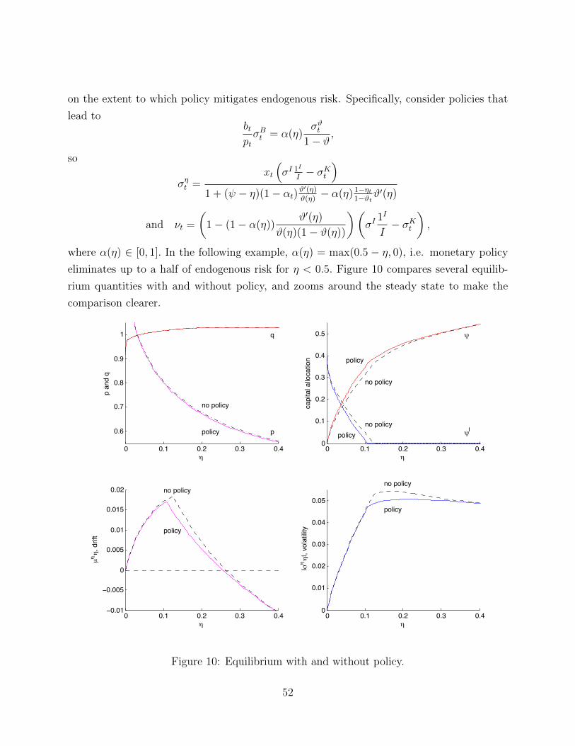
on the extent to which policy mitigates endogenous risk. Specifically, consider policies that

lead tobtptσBt = α(η)

σϑt1− ϑ

,

so

σηt =xt

(σI 1I

I− σKt

)1 + (ψ − η)(1− αt)ϑ

′(η)ϑ(η)− α(η) 1−ηt

1−ϑtϑ′(η)

and νt =

(1− (1− α(η))

ϑ′(η)

ϑ(η)(1− ϑ(η))

)(σI

1I

I− σKt

),

where α(η) ∈ [0, 1]. In the following example, α(η) = max(0.5 − η, 0), i.e. monetary policy

eliminates up to a half of endogenous risk for η < 0.5. Figure 10 compares several equilib-

rium quantities with and without policy, and zooms around the steady state to make the

comparison clearer.

0 0.1 0.2 0.3 0.4

0.6

0.7

0.8

0.9

1

η

p an

d q

no policy

policy p

q

0 0.1 0.2 0.3 0.4−0.01

−0.005

0

0.005

0.01

0.015

0.02

η

µη η

, drif

t

policy

no policy

0 0.1 0.2 0.3 0.40

0.1

0.2

0.3

0.4

0.5

η

capi

tal a

lloca

tion

ψI

ψ

no policy

no policypolicy

policy

0 0.1 0.2 0.3 0.40

0.01

0.02

0.03

0.04

0.05

η

|ση η

|, vo

latil

ity

no policy

policy

Figure 10: Equilibrium with and without policy.

52

The bottom right panel illustrates that policy reduces risk. As a result, intermediaries

are able to employ their technologies to a greater extent even for lower levels of net worth,

and households step in to inefficiently use the intermediaries’ technologies at a lower level

of ηt - see top right panel. At the same time, intermediaries are able to maintain higher

leverage - their net worth at the steady state is reduced as shown in the bottom left panel.

The top left panel shows that the value of money is somewhat lower with the policy - due

to the fact that intermediaries are able to function more efficiently and create more inside

money. The price of capital q(η) does not change significantly (it becomes slightly higher

with the policy).

0 0.2 0.4 0.6 0.8−240

−235

−230

−225

−220

−215

−210

−205

−200

tota

l wel

fare

mea

sure

(das

hed:

no

polic

y, s

olid

: pol

icy)

η0 0.2 0.4 0.6 0.8

−90

−85

−80

−75

−70

−65

−60

−55

−50

η

utilit

y, p

er u

nit o

f net

wor

th (d

ashe

d: n

o po

licy,

sol

id: p

olic

y)

intermediaries

households

Figure 11: Welfare in Equilibrium.

Figure 11 confirms that this policy, though appropriate risk transfer, indeed improves

welfare. It replicates Figure 5, and compares welfare measures with and without policy.

Overall welfare clearly improves with policy, as we can see from the right panel of Figure 11.

Moreover, total welfare is maximized at a lower level of η, so that the shift of the steady state

to the left is not detrimental. We estimated that this improvement in welfare is equivalent to

increased consumption by about 9% per year. The left panel shows the effect on individual

agents. Households get slightly lower utility given any wealth level with policy, but also at

the steady state they have greater wealth.

53

Compare with

ρω(η) = log(ρp(η)) +Φ(ι(η))− δ − ρ− σ2/2

ρ+ ω′(η)µηt η +

ω′′(η)η2σηt (σηt )T

2.

Let H0(η) = ω(ηt)− log(pt)/ρ. Then this agent’s utility can be also expressed as H0(ηt)+

log(nt)/ρ, where H0 satisfies the HJB equation

ρH0(ηt) = log(ρ) +1

ρE

[dntnt

]/dt− (σpt + σKt )2

2ρ+H ′0(η)µηt η +

H ′′0 (η)η2σηt (σηt )T

2. (5.19)

Now, consider another agent whose best investment opportunity over money has risk νt

and who (given the returns) chooses to put portfolio weight xt on this opportunity. Then

this agent’s wealth follows

dntnt

=dntnt

+ xtνt(xtνt + σpt + σKt )T dt+ xtνt dZt.

The utility of this agent can be represented in the form H(ηt) + log(nt)/ρ, where

ρH(ηt) = log(ρ) +1

ρE

[dntnt

]/dt+

xtνt(xtνt + σpt + σKt )T

ρ

−|σpt + σKt |2

2ρ− xtνt(σ

pt + σKt )T

ρ− x2

tνtνTt

2ρ+H ′(η)µηt η +

H ′′(η)η2σηt (σηt )T

2.

Subtracting (5.19), we find that the difference in the utilities of these two agents, h(ηt) =

H(η)−H0(η), satisfies the ordinary differential equation

ρh(η) =x2tνtν

Tt

2ρ+ h′(η)µηt η +

h′′(η)η2σηt (ση)T

2. (5.20)

6 Conclusion

We consider an economy in which household entrepreneurs and intermediaries make invest-

ment decisions. Household entrepreneurs can invest only in a single real production tech-

nology at a time, while intermediaries have the expertise to invest in a number of projects.

In equilibrium intermediaries take advantage of their expertise to diversify across several

investment projects. They scale up their activity by issuing demand deposits, inside money.

54

Households hold this inside money in addition to outside money provided by the government.

Intermediaries are leveraged and assume liquidity mismatch. Intermediaries’ assets are long-

dated and have low market liquidity - after an adverse shock the price can drop - while their

debt financing is short-term. Endogenous risk emerges through amplification mechanism in

form of two spirals. First, the liquidity spiral: a shock to intermediaries causes them to

shrink balance sheets and “fire sale some of their assets”. This depresses the price of their

assets which induces further fire-sales and so on. Second, the disinflationary spiral: as inter-

mediaries shrink their balance sheet, they also create less inside money; such a shock leads

to a rising demand for outside money, i.e. disinflation. This disinflationary spiral amplifies

shocks, as it hurts borrowers who owe nominal debt. It works on the liabilities side of the

intermediary balance sheets, while the liquidity spiral that hurts the price of capital works on

the asset side. Importantly, in this economy the money multiplier, the ratio between inside

and outside money, is endogenous: it depends on the health of the intermediary sector.

Monetary policy can mitigate the adverse effects of both spirals in the presence of default-

free long-term government bonds. Conventional monetary policy changes the path of interest

rate earned on short-term money and consequently impacts the relative value of long-term

government bond and short-term money. For example, interest rate cuts in downturns that

are expected to persist for a while enable intermediaries to refinance their long-bond holding

more cheaply. This recapitalizes institutions that hold these assets and and also increases

the (nominal) supply of the safe asset. The resulting reduction in endogenous risk leads

to welfare improvements. Of course, any policy that provides insurance against downturns

could potentially create moral hazard. Indeed, intermediaries take on higher leverage, but

more hazard is limited. The reason is that the “stealth recapitalization” through a persistent

interest rate cut not only recapitalizes institutions with high leverage because they funded

many real projects but also the ones which simply held long-term (default-free) Government

bonds. The finding that moral hazard is limited might change if one were to include inter-

mediaries with negative net worth. Including zombie banks is one fruitful direction to push

this line of research further.

7 Bibliography

Bernanke, B. (1983) “Non-Monetary Effects of the Financial Crisis in the Propagation

of the Great Depression”, American Economic Review, Vol. 73, 257-276.

Bernanke, B. and A. Blinder (1989) “Credit, Money, and Aggregate Demand”, American

55

Economic Review, Papers and Proceedings, Vol. 78, No. 2, 435-439.

Bernanke, B. and M. Gertler (1989) “Agency Costs, Net Worth, and Business Fluctua-

tions”, American Economic Review, Vol. 79, No. 1, 14-31.

Bernanke, B., M. Gertler and S. Gilchrist (1999) “The Financial Accelerator in a Quan-

titative Business Cycle Framework”, Handbook of Macroeconomics (Chapter 21), 1341-1393.

Bewley, T. (1980) “The Optimum Quantity of Money”, in Models of Monetary Eco-

nomics, eds. J. Kareken and N. Wallace. Minneapolis, Minnesota: Federal Reserve Bank.

Brunnermeier, M. K., T. Eisenbach, and Y. Sannikov (2013) “Macroeconomics with

Financial Frictions: A Survey”, in Proceedings of the Econometric Society World Congress

2010 in Shanghai, eds. E. Dekkel, Cambridge University Press.

Brunnermeier, M. K. and Y. Sannikov (2014) “A Macroeconomic Model with a Financial

Sector”, American Economic Review, 104(2), 379-421.

Brunnermeier, M. K. and Y. Sannikov (2013) “Redistributive Monetary Policy”, Jackson

Hole Symposium 2012.

Cagan, P. (1979) Persistent Inflation: Historical and Policy Essays, Columbia university

Press.

Christiano, L., R. Moto and M. Rostagno (2003) “The Great Depression and the Friedman-

Schwartz Hypothesis”, Journal of Money, Credit and Banking, 35(6), 1119-1197.

Curdia, V. and M. Woodford (2010) “Credit Spreads and Monetary Policy”, working

paper, Columbia University.

Diamond, D. W. (1984) “Financial Intermediation and Delegated Monitoring”, The Re-

view of Economic Studies, 51(3), 393-414.

Diamond, D. and R. Rajan (2006) “Money in a Theory of Banking”,’ American Economic

Review, March 2006.

Fisher, I. (1933), “The Debt-Deflation Theory of Great Depression”, Econometrica, Vol.

1, No. 4, October 1933, 337-357.,

Friedman, M. and A. J. Schwartz. (1963) A Monetary History of the United States,

1867-1960, Princeton University Press.

Gurley, J. and E. Shaw (1955) “Financial Aspects of Economic Development”, American

Economic Review, September 2006, 515-538.

Gertler, M. and Karadi (2014) “Monetary Policy Surprises, Credit Costs and Economic

Activity”, American Economic Journal: Macroeconomics, forthcoming.

56

Hahn, F. H. (1973) “On the Foundation of Monetary Theory”, in: M. Parkin and A. R.

Nobay, eds., Essays in Modern Economics, Barnes and Noble, New York, NY, 230-242.

Hanson, S. G., and J. C. Stein. (2014) “Monetary Policy and Long-Term Real Rates.”

Working Paper, April 2014.

Hart, O. (1975). “On the Optimality of Equilibrium When the Market Structure Is

Incomplete.? Journal of Economic Theory 11: 418-443.

He, Z., and A. Krishnamurthy (2013) “Intermediary Asset Prices”, American Economic

Review, 103(2), 732-770.

He, Z., and A. Krishnamurthy (2012) “A Model of Capital and Crises”, Review of Eco-

nomic Studies., 79(2), 735-777.

Holmstrom, B., and J. Tirole (1997): “Financial Intermediation, Loanable Funds, and

the Real Sector”, The Quarterly Journal of Economics, 112(3), 663-691.

Kiyotaki, N. and J. Moore (1997) “Credit Cycles”, Journal of Political Economy, Vol.

105, No. 2, 211-48.

Kiyotaki, N. and J. Moore (2008) “Liquidity, Business Cycles, and Monetary Policy”,

working paper, Princeton University.

Levin, D. K. (1991) “Asset Trading Mechanism and Expansionary Policy”, Journal of

Economic Theory, Vol. 54, No. 1, 148-164.

Lippi, F. and N. Trachter (2012) “On the Optimal Supply of Liquidity with Borrowing

Constraints”, working paper, EIEF.

Mendoza, E. and K. A. Smith (2006) “Quantitative Implications of a Debt-Deflation

Theory of Sudden Stops and Asset Prices”, Journal of International Economics, Vol. 70,

No. 1, 82 - 114.

Patinkin D. (1965) Money, Interest and Prices: An Integration of Monetary and Value

Theory, Harper & Row NY.

Samuelson, P. A. (1958) “An exact consumption loan model of interest, with or without

the social contrivance of money” Journal of Political Economy 66, 467-82.

Stein, J. (2012) “Monetary Policy as Financial-Stability Regulation”, Quarterly Journal

of Economics 127(1), 57-95.

Scheinkman, J. A. and L. Weiss (1986) “Borrowing Constraints and Aggregate Economic

Activity”, Econometrica, Vol. 54, 23-45

57

Tobin, J. (1969) “A General Equilibrium Approach to Monetary Theory”, Journal of

Money, Credit and Banking, Vol. 1, No. 1, 15-29.

Wallace, Neil, “A Modigliani-Miller Theorem for Open-Market Operations”, American

Economic Review 71: 267-274 (1981).

Williamson, S. and R. Wright (2011) “New Monetarist Economics: Models,” in Handbook

of Monetary Economics, Vol. 3A, B. Friedman and M. Woodford, eds., Elsevier.

58

A Numerical Procedure to find Equilibrium

(to be completed)

Computational Procedure. The function ϑ(η) can be determined by a second-order

differential equation, and the following procedure provides a way to find ϑ′′(η) from (η, ϑ(η), ϑ′(η)).

First, we have to guess variables ψ and χ characterizing the allocation of capital and equity

issuance, which satisfy the following conditions. Given ψ and χ, letting w = σa1a− σb1b, we

have

σηt η =xtη(1− ψ)

1 + (ψ(1− χ)− η)(1− α)ϑ′(η)ϑ(η)− (1− η)α ϑ′(η)

1−ϑ(η)︸ ︷︷ ︸χη

w,

σϑ =ϑ′(η)

ϑ(η)χη︸ ︷︷ ︸

χϑ

w, σβ =α

1− ϑχϑ︸ ︷︷ ︸

χβ

w,

ν =

(1− ψ − χϑ

1− ϑ+ χβ

)︸ ︷︷ ︸

χν

w, νb =

(−ψ − χϑ

1− ϑ+ χβ

)︸ ︷︷ ︸

χν,b

w.

Define xt = ψt(1−χt)(1−ϑt)/ηt, and solve for household leverage xat and xbt from the relative

pricing and indifference conditions

Aa(ψt)− Ab(ψt)qt

− χϑ

1− ϑw2 = wσK − χβw2

+(1− χt)(xt(χν)2 +ϑ

ηχβχν)w2 + χtx

at ((χ

ν)2w2 + σ2)− xbt((χν,b)2w2 + σ2)

and (xat )2((χν)2w2 + σ2) = (xbt)

2((χν,b)2w2 + σ2).

The guesses of ψ and χ are correct if

χν(xtχν +

ϑ

ηχβ)w2 ≥ xat ((χ

ν)2w2 + σ2), with strict inequality if χt = χ

andψtχtxat

+1− ψtxbt

=1− ηt1− ϑt

.

Finally, find

59

µϑ = (1− ϑ)

(Ab(ψt)− ιt

qt+

(χϑ)2w2

1− ϑ− σ2

bχϑ

1− ϑ+ χβ(xtχ

ν +ϑ

ηχβ)w2+(

ψb − 1− χϑ

1− ϑ

)(χβw2 − wσK)− xbt((χν,b)2w2 + σ2)

)

µηη = η(1− η)

((xtχ

ν +ϑ

ηχβ)2w2 − (xbt)

2((χν,b)2w2 + σ2)

)+ χη

(χϑ − χβ

)w2

and ϑ′′(η) =2(µϑϑ(η)− µηηϑ′(η))

(χη)2w2.

Procedure. The function ϑ(η) that results under any policy that removes endogenous

risk according to (5.13) has to satisfy the following second-order differential equation. First,

given η and (ϑ(η), ϑ′(η)) the allocation of capital (ψt, ψJt ) must satisfy the conditions

xt =ψt(1− ϑ(η))

ηt, σηt =

xt

(σI 1I

I− σKt

)1− 1−ηt

1−ϑt ϑ′(η)

, σϑt =ϑ′(η)

ϑ(η)σηt η, Y − ι(q) =

ρq

1− ϑ(η),

xt|νt|2 +νtϑtηt

(σϑ)T

1− ϑ= xIt |νIt |2,

(P it − P

jt )a

qt= (σI1i−σJ1j)(σKt )T +xIt |νIt |2−xJt |νJt |2. (A.1)

η +ψJ(1− ϑ(η))

xJt︸ ︷︷ ︸ηJ

+(1− ψJ − ψ)(1− ϑ(η))

xIt︸ ︷︷ ︸ηI

= 1 and (xIt )2|νIt |2 ≤ (xJt )2|νJt |2,

with equality of ψ + ψJ < 1. Then,

P It a− ιq

+σϑ

1− ϑσηt = νt

(σηt +

ϑtσϑ

1− ϑt+ σKt

)T+

µϑ

1− ϑ(A.2)

and ϑ′′(η) =µϑϑ(η)− ϑ′(η)µηt η

η2σηt (σηt )T/2,

where the volatility of η, µηt , is taken from (5.14).

Proof. We only need to justify the expressions that appear in the above procedure for the

60

first time. Note that

σNt = σKt + σpt −btptσBt︸ ︷︷ ︸

σMt =σKt +σqt

+xt

(σI

1I

I− σKt

)+ϑtηt

σϑ

1− ϑ,

Subtracting the capital pricing conditions for intermediaries and households who hold capital

types i = 1, . . . I, we obtain

xt|νt|2 + νtϑtηt

(σϑ)T

1− ϑ= xIt |νIt |2,

since νt(σMt )T = νit(σ

Mt )T . Furthermore, the capital pricing conditions of intermediaries and

households who hold capital types j = I + 1, . . . I + J, we find

(P it − P

jt )a

qt+ (σIt 1

i − σjt1j)(σqt )T = xIt |νIt |2 − xJt |νJt |2 + (σIt 1

i − σJt 1j)(σKt + σqt )T ,

which simplifies to the second equation in (A.1).

Finally, from the capital and bond pricing conditions for intermediaries, we obtain

E[drIt − drMt ]

dt=P It a− ιq

+ µqt − µpt + σqt

(σI

1I

I

)T− σpt (σKt )T +

σϑ

1− ϑ(σNt )T = νtσ

Nt

Since

σNt = σηt +ϑtσ

ϑ

1− ϑt+ σMt and

µpt − µqt =

σϑ

1− ϑσp − (σϑ)2

1− ϑ+

µϑ

1− ϑ, σpt − σ

qt =

σϑt1− ϑ

,

we haveP It a− ιq

+σϑ

1− ϑσηt = νt

(σηt +

ϑtσϑ

1− ϑt+ σKt

)T+

µϑ

1− ϑ,

as required.

61

B Proofs

Proof of Proposition 1. Consider the law of motion of net worth

dntnt

= µnt dt+σnt dZt = drMt −ρdt+

{xat (ν

at )T ((xat ν

at + σMt ) dt+ dZt) + xat σ

a(xat σa dt+ dZt)

xbt(νbt )T ((xbtν

bt + σMt ) dt+ dZt) + xbt σ

b(xbt σb dt+ dZt),

depending on whether the household employs technology a or b.

According to (3.6), the household gets the same utility from any choice over these two

technologies if and only if µnt − |σnt |2/2 is the same for both technologies. For technology a,

this is

E[drMt ]

dt− ρ+ (xat )

2(|νat |+ (σa)2) + xat (νat )TσMt −

|xat νat + σMt |2 + (xat σa)2

2=

E[drMt ]

dt− ρ+

(xat )2(|νat |+ (σa)2)− |σMt |2

2.

Equating this for technologies a and b, we obtain the indifference condition (2.12).

Lemma 1. Suppose that η = 0, i.e. there are no intermediaries. The equilibrium is charac-

terized by a single equation for the allocation ψ of capital to technology b

Aa(ψ)− Ab(ψ)

q=

ρ

xa− ρ

xb+ (1− ψ)(σa)2 − ψ(σb)2, (B.1)

with the remaining quantities expressed as

xa =

√ρ

ψ2((σa)2 + (σb)2) + (σa)2, xb =

√ρ

(1− ψ)2((σa)2 + (σb)2) + (σb)2, (B.2)

1− ϑ =xaxb

(1− ψ)xb + ψxaρq

1− ϑ= A(ψ)− ι(q) and p =

ϑ

1− ϑq. (B.3)

Proof. The aggregate risk of capital is σK dZt = (1 − ψ)σa1a dZat + ψσb1b dZb

t , incremental

aggregate risks from exposures to technologies a and b are

νat = ψ(1aσa − 1bσb) dZt, νbt = (1− ψ)(1bσb − 1aσa) dZt,

62

and the risk exposure of households in sectors a and b are

xaνat dZt + σK dZt + xaσa dZt and xbνbt dZt + σK dZt + xbσb dZt,

respectively. Hence, household indifference condition is

X ≡ (xa)2(ψ2((σa)2 + (σb)2)︸ ︷︷ ︸|νat |2

+(σa)2) = (xb)2((1− ψ)2((σa)2 + (σb)2)︸ ︷︷ ︸|νbt |2

+(σb)2). (B.4)

The asset-pricing conditions for capital employed in sectors a and b are

Aa(ψ)− ιq

= xa(|νat |2 + (σa)2) + ψ((1− ψ)(σa)2 − ψ(σb)2) and

Ab(ψ)− ιq

= xb(|νbt |2 + (σb)2) + (1− ψ)(ψ(σb)2 − (1− ψ)(σa)2).

Adding up these two equations with coefficients 1−ψ and ψ, and using the market-clearing

condition for capital, we obtain

ρ

1− ϑ=

(1− ψxa

+ψ

xb

)︸ ︷︷ ︸

1/(1−ϑ) by (2.14)

X ⇒ X = ρ.

This, together with (B.4), implies (B.2).

Equations in (B.3) follow from (2.14), market clearing condition for output and the

definition of ϑ.

Finally, the difference between the asset-pricing conditions is

Aa(ψ)− Ab(ψ)

q= xa(|νat |2 + (σa)2)︸ ︷︷ ︸

ρ/xa

−xb(|νbt |2 + (σb)2)︸ ︷︷ ︸ρ/xb

+(1− ψ)(σa)2 − ψ(σb)2.

This yields (B.1).

Proof of Proposition 3. Notice that

ns = nt exp

(∫ s

t

(µns′ −

|σns′ |2

2

)ds′ +

∫ s

t

σns′ dZt

),

since Ito’s lemma implies that then process ns satisfies (3.5) as required.

63

Hence,

Et[log(ρns)] = log(ρnt) + Et

[∫ s

t

(µns′ −

|σns′ |2

2

)ds′].

Integrating over [t,∞) and discounting, we obtain

Et

[∫ ∞t

e−ρ(s−t) log(ρns) ds

]=

log(ρnt)

ρ+ Et

[∫ ∞t

e−ρ(s−t)∫ s

t

(µns′ −

|σns′ |2

2

)ds′ ds

],

which yields (3.6) after changing the order of integration.

Proof of Proposition 5. Let us normalize K0 = 1. Consider an economy, in which households

are required to allocate fraction ϑ ∈ [0, 1) of their wealth to money. Then, from the market-

clearing condition for consumption goods, if Φ(ι) = log(κι+ 1)/κ, then

A− ι(q) = ρ (p+ q)︸ ︷︷ ︸q/(1−ϑ)

⇒ q =(κA+ 1)(1− ϑ)

κρ+ 1− ϑand Φ(ι) =

log(q)

κ.

Then (3.7) implies that, given policy,

µn = Φ(ι)− δ, |σn|2 = (1− ϑ)2σ2 + σ2,

hence welfare (3.6) is

log(ρ(p+ q))

ρ+µn − |σn|2/2

ρ2=

log(ρ) + log(q/(1− ϑ))

ρ+

log(q)/κ− δ − (1− ϑ)2σ2/2− σ2/2

ρ2

=log(ρ)

ρ− δ + σ2/2

ρ2+κρ+ 1

κρ

(log(κA+ 1)

ρ− log(κρ+ 1− ϑ)

ρ

)+

log(1− ϑ)

κρ2− (1− ϑ)2σ2

2ρ2

Let us show that welfare in the equilibrium with money is greater than in that without

money. In the equilibrium with money 1− ϑ =√ρ/σ, so we need to show that

−κρ+ 1

κρlog(κρ+

√ρ/σ) +

1

κρlog(√ρ/σ)− 1

2≥ −κρ+ 1

κρlog(κρ+ 1)− σ2

2ρ⇔

−κρ+ 1

κρlog(κρx+ 1) + log x+

x2

2≥ −κρ+ 1

κρlog(κρ+ 1) +

1

2(B.5)

where x = σ/√ρ > 1. If we set x = 1, the two sides are equal. Differentiating the left-hand

64

side with respect to x we obtain

1− x(κρx+ 1)x

+ x ≥ 1− xx

+ x =1− x+ x2

x> 0.

Hence (B.5) holds for all x > 1, i.e. the equilibrium with money is strictly better.

Now, consider the optimal policy. Differentiating welfare with respect to ϑ we get

κρ+ 1

κρ2

1

κρ+ 1− ϑ− 1

κρ2(1− ϑ)+

(1− ϑ)σ2

ρ2=

−1

ρ

ϑ

(κρ+ 1− ϑ)(1− ϑ)+

(1− ϑ)σ2

ρ2=

1

ρ(1− ϑ)

(−ϑ

κρ+ 1− ϑ+

(ϑ− 1)2σ2

ρ

),

where the term in parentheses is increasing in ϑ. For the equilibrium level of ϑ = 1−√ρ/σ,this term becomes √

ρ/σ − 1

κρ+√ρ/σ

+ 1 =2√ρ/σ − 1 + κρ

κρ+√ρ/σ

,

positive if and only if 2√ρ/σ > 1 − κρ. Thus, the welfare-maximizing policy raises ϑ over

the equilibrium level if and only if condition (3.9) holds.

Alternative Proof of Proposition 9. Money has risk σMt = σKt + σpt − bt/pt σBt . Effectively,

risk bt/pt σBt is subtracted from money and is allowed to be traded separately, carrying the

risk premium of bt/pt (σBt )TσNt , since it is the intermediaries that hold bonds. The net worth

of intermediaries follows

dNt

Nt

= drMt − ρ dt+ (xtνbt + xBt σ

Bt )T (σNt dt+ dZt), where xBt =

btηt(pt + qt)

.

World wealth follows

d((qt + pt)Kt)

(qt + pt)Kt

= drMt − ρ dt− (σϑt )T (σMt dt+ dZt) + ηt(xBt σ

Bt )T (σNt dt+ dZt)︸ ︷︷ ︸

bonds in the world portfolio

+ηt xt(νbt )T (xtν

bt + xBt σ

Bt )︸ ︷︷ ︸

risk premium adjustment

dt+ (1− ηt)(xat )2(|νat |2 + (σa)2) dt,

where we adjusted equation (2.17) for the presence of bonds in the world portfolio, as well

as for the effect of bonds on the risk premium demanded by intermediaries.

65

Therefore, using Ito’s lemma,

dηtηt

= (1− ηt)(|xtνbt + xBt σBt |2 − (xat )

2(|νat |2 + (σa)2)) dt+

(xtνbt + σϑt + (1− ηt)xBt σBt )T (dZt + (σθt − ηtxBt σBt ) dt).

Proof of Proposition 9. The law of motion of total net worth of intermediaries, given the

risks that they take, must be

dNt

Nt

= drMt − ρ dt+ (xtνbt + xBt σ

Bt )T (σMt dt+ dZt) + |xtνbt + xBt σ

Bt |2 dt.

The law of motion of world wealth (qt + pt)Kt can be found from the total return on world

wealth, after subtracting the dividend yield of ρ (i.e., aggregate consumption). To find the

returns, we take into account the risk premia that various agents have to earn. We have

d((qt + pt)Kt)

(qt + pt)Kt

= drMt − ρ dt+ (1− ϑt)(σqt − σpt )T︸ ︷︷ ︸

−(σϑt )T

dZt + ηt(xBt σ

Bt )T (σNt dt+ dZt)+

(1− ϑt)((1− ψt) ((νat )TσNat + xat (σa)2)︸ ︷︷ ︸

Et[drat −dr

Mt ]

dt

+ψt(χt(ν

bt )TσNt + (1− χt)((νbt )TσNbt + xbt(σ

b)2))︸ ︷︷ ︸

Et[drbt−dr

Mt ]

dt

) dt

Recall that

σNt = xtνbt + xBt σ

Bt + σMt , σNat = xat νt + σMt and σNbt = xbtν

bt + σMt ,

(1− ψt)νat + ψtνbt = σqt − σ

pt ,

(1− ϑt)(

1− ψtxat

+ψtxbt

)= 1− ηt and (xat )

2(|νat |2 + (σa)2) = (xbt)2(|νbt |2 + (σb)2).

Therefore, the law of motion of aggregate wealth can be written as

d((qt + pt)Kt)

(qt + pt)Kt

= drMt − ρ dt− (σϑt − ηtxBt σBt )T (σMt dt+ dZt)+

66

(1− ηt)(xat )2(|νat |2 + (σa)2) dt+ ηt|xtνbt + xBt σBt |2 dt.

Thus, using Ito’s lemma, we obtain.15

dηtηt

= (xtνbt + xBt σ

Bt + σϑt − ηtxBt σBt )T (σMt dt+ dZt)+

(1− ηt)|xtνbt + xBt σBt |2 dt− (1− ηt)(xat )2(|νat |2 + (σa)2) dt

−(xtνbt + xBt σ

Bt + σϑt − ηtxBt σBt )T (σMt − σϑt + ηtx

Bt σ

Bt ) dt =

(1− ηt)(|xtνbt + xBt σ

Bt |2 − (xat )

2(|νat |2 + (σa)2))dt+

(xtνbt + xBt σ

Bt + σϑt − ηtxBt σBt )T (dZt + (σϑt − ηtxBt σBt ) dt).

Notice that

νbt = 1bσb +σqt −σMt = 1bσb +σqt −σpt −σKt +

btptσBt = (1−ψt)(1bσb− 1aσb)− σϑt

1− ϑ+btptσBt =

(1− ψt)(1bσb − 1aσb)− ϑ′(η)

ϑ(1− ϑ)ησηt +

btpt

B′(η)

Bησηt .

Hence, σηt equals

xt(1− ψt)(1bσb − 1aσb)− xtϑ′(η)

ϑ(1− ϑ)ησηt + xt

btpt

B′(η)

Bησηt +

ϑ′(η)

ϑησηt + ϑt

1− ηtηt

btpt

B′(η)

Bησηt

= xt(1− ψt)(1bσb − 1aσb)−(

(χtψt − ηt)ϑ′(η)

ϑ− (χtψt(1− ϑt) + ϑt(1− ηt))

btpt

B′(η)

B

)σηt

15If processes Xt and Yt follow

dXt/Xt = µXt dt+ σXt dZt and dYt/Yt = µYt dt+ σYt dZt,

thend(Xt/Yt)

Xt/Yt= dXt/Xt − dYt/Yt − (σXt − σYt )TσYt dt.

67

It follows that

σηt =xt(1− ψt)(1bσb − 1aσb)

1 + (χtψt − ηt)ϑ′(η)ϑ− (χtψt(1− ϑt) + ϑt(1− ηt)) btpt

B′(η)B

.

Proof of Proposition 10. Equation (5.7) follows directly from Ito’s lemma. Let us justify the

remaining six equations.

Relative to money, capital devoted to the production of good a earns the return of

drat − drMt =Aa(ψt)− ιt

qtdt+ (µqt − µ

pt ) dt+ (σa1a − σKt )T dZt + σa dZt.

Likewise,

drbt − drMt =Ab(ψt)− ιt

qtdt+ (µqt − µ

pt ) dt+ (σb1b − σKt )T dZt + σb dZt.

Fraction 1 − χ of the risk of good a is borne by intermediaries, who are exposed to

aggregate risk σKt , and fraction χ, by households, who are exposed to aggregate risk σKt and

idiosyncratic risk xat σa. Thus,

Aa(ψt)− ιtqt

+ µqt − µpt = (σa1a − σK)TσK + χ xat (σ

a)2, (B.6)

where (σa1a−σK)TσK is the risk premium for aggregate risk of this investment, and χxat (σa)2

is the price of idiosyncratic risk. For good b,

Ab(ψt)− ιtqt

+ µqt − µpt = (σb1b − σK)TσK + xbt(σ

b)2. (B.7)

Now, since any investment in capital will include a hedge for the aggregate risk component,

νt = νbt = 0,

so the indifference condition of households (2.12) becomes, one,

(xat )2(σa)2 = (xbt)

2(σb)2 ⇔ xat = xbtσb

σa,

68

and the law of motion of ηt is, two,

dηtηt

= −(1− ηt)(xbt)2(σb)2 dt, (B.8)

From (2.14), we have, three,ψtχ

xat+

1− ψtxbt

=1− ηt1− ϑt

. (B.9)

ψtχ σa/σb + 1− ψt = xb

1− ηt1− ϑt

.

Subtracting (B.7) from (B.6), we get, four,

Aa(ψt)− Ab(ψt)qt

= (σa1a − σb1b)TσK + χxat (σa)2 − xbt(σb)2. (B.10)

The market-clearing condition for consumption goods is, five,

A(ψt)− ι(qt) =ρqt

1− ϑt.

Finally, taking a weighted average of (B.6) and (B.7), with weights ψ and 1− ψ, we have

A(ψ)− ιtqt︸ ︷︷ ︸

ρ/(1−ϑt)

+µqt − µpt = (χψ σa/σb + 1− ψ)xbt(σ

b)2.

This, in combination with (B.9), and the identity µϑt = (1 − ϑt)(µpt − µqt ) − σϑσp + (σϑ)2,

leads to the last equation, (5.8), six.

C “As If ” Representative Agent Model

Salient features of the various equilibria discussed above can also be achieved through closely

related representative agent economies. Suppose the representative agent is endowed with

initial capital K0 ≡∫ 1

0ki0di and that he faces technology-specific, but no purely idiosyncratic

risk. Let us furthermore assume that this representative agent also has log preferences, but

now with discount factor ρ. For starters, suppose that he can only invest in technologies a

or b (no money is available). In that case his portfolio problem is simple: He will consume a

constant fraction ρ of his wealth, he will invest equal fractions of his capital at each instant

69

in technologies a and b, and the price of capital will be time-invariant and satisfy

qR =κA+ 1

κρ+ 1

For ρ = ρ we exactly recover the no-money equilibrium above, with the sole difference

that welfare of the representative households exceeds welfare of the atomistic households

above (since the representative household need not bear any idiosyncratic risk). A formal

analysis of the welfare difference will follow in the next section. It is also instructive to

consider the case ρ =√ρσ. In that case, the equilibrium with the representative agent is, as

far as real quantities and the price of capital are concerned, exactly the same as the money

equilibrium above. Since ρ > ρ, we see that the money equilibrium effectively amounts to

an decrease in patience.

Finally, it is interesting to consider the question of whether money can have value in a

representative agent economy. Evidently, the answer is no – an asset that never generates

any real payoff cannot be held in positive quantities forever without violating the investor’s

transversality condition. However, let us for the moment assume that the transversality

condition is allowed to be violated. In that case, as long as the representative household has

no purely idiosyncratic risk, there still could be no equilibrium with constant p, q � 0, for

money would be a strictly dominated asset. We could of course deal with strict dominance by

re-introducing idiosyncratic risk, but then the aggregate law of motion for capital would be

different (since now idiosyncratic cannot cancel in the aggregate). Only if the representative

agent would perceive the threat of idiosyncratic risk at every period, but without this risk

every materializing, would we recover allocations and prices from the money equilibrium

above – and all of course subject to the proviso of ignoring the representative household’s

transversality condition.

D Old Material

D.1 Welfare Analysis, No Intermediaries

What if the regulator can control ϑ by forcing the agents to hold specific amounts of money?

In this case, we have to use the economy-size method which directly takes into account the

cost idiosyncratic risk exposure, without assuming that agents earn the required return for

70

the risk that they take.16 Since the choice of ϑ will affect asset prices, and thus wealth, we

can calculate welfare per unit of capital in the economy to be

D.2 OLD Welfare, with Intermediary Sector

The Investment Return Method. The following proposition evaluates the welfare of any

agent as a function of his/her investment opportunities.

Proposition 13. The welfare of an agent with wealth nt who can invest only in money takes

the form hM(ηt) + log(ρnt)/ρ, where hM(ηt) satisfies

hM(ηt) +log ptρ

= Et

[∫ ∞t

e−ρ(s−t)(

log(ps) +Φ(ιs)− δ − ρ− |σKs |2/2

ρ

)ds

](D.1)

The welfare of an intermediary with net worth nt is hI(ηt) + log(ρnt)/ρ, where

hI(ηt)− hM(ηt) = Et

[∫ ∞t

e−ρ(s−t)x2s|νbs|2

2ρds

](D.2)

The welfare of a household is hH(ηt) + log(ρnt)/ρ, where hH(ηt)− hM(ηt) satisfies equation

(D.2) with the term x2s|νbs|2 replaced by (xbs)

2(|νbs|2 + (σb)2).

Equation (D.2) evaluates the welfare of an individual agent by inferring the Sharpe ratio

that the agent earns on risky investment from the risk that the agent chooses to take. The

expectations (D.1) and (D.2) can be found numerically through an ordinary differential

equation, since

g(ηt) = Et

[∫ ∞t

e−ρ(s−t)y(ηs) ds

]⇒ ρg(η) = y(η) + g′(η)µηt η +

g′′(η)|ησηt |2

2. (D.3)

Throughout the proofs we also make use of the following identity

ρg(ηt) = y(ηt) + Et[dg(ηt)]/dt ⇒ g(ηt) = Et

[∫ ∞t

e−ρ(s−t)y(ηs) ds

]. (D.4)

Note that, given the form of equation (D.2), it makes sense why Proposition 1 gives the

right condition for the household to be indifferent between the production of goods a and b.

16When the regulator controls portfolios, it is no longer true that the excess return of any risky asset overany other asset is explained by their covariance with the agent’s net worth.

71

Under condition (2.12), the household has the same welfare regardless of the technology it

chooses to pursue.

Proof. With log utility, if the wealth of the agent increases by a factor of y, then his/her utility

increases by log(y)/ρ, since the agent increases consumption by a factor of y in perpetuity

and keeps portfolio weights the same.

We can write the utility of an agent with wealth nt who can invest only in money in the

form hM(ηt) + log(ρ)/ρ+ log(nt)/ρ, and if we express nt = ptkt, then

dktkt

= (Φ(ιt)− δ − ρ) dt+ σKt dZt,

since the agent consumes at rate ρ. Then the agent’s utility has to satisfy the equation

ρ

(hM(ηt) +

log(ρnt)

ρ

)= log(ρnt) +

Et[d(hM(ηt) + log(kt)/ρ+ log(pt)/ρ

)]dt

⇒

ρ

(hM(ηt) +

log(pt)

ρ

)= log(pt) +

Φ(ιt)− δ − ρρ

− |σKt |2

2ρ+Et[d(hM(ηt) + log(pt)/ρ

)]dt

so (D.4) implies that hM(η) + log(pt)/ρ satisfies (D.1).

The net worth of this agent follows dnt/nt = drMt − ρ dt, and recall that the net worth

of an intermediary follows (2.16), i.e.

dnItnIt

= drMt − ρ dt+ xt(νbt )T ((xtν

bt + σMt )︸ ︷︷ ︸σNt

dt+ dZt).

If we write the utilities of these agents as hMt + log(ρnt)/ρ and hIt + log(ρnIt )/ρ then we have

ρ

(hMt +

log(ρnt)

ρ

)= log(ρnt) +

1

ρEt

[dntnt

]/dt− |σ

Mt |2

2ρ+ Et[dh

Mt ]/dt and

ρ

(hIt +

log(ρnIt )

ρ

)= log(ρnIt ) +

1

ρEt

[dnItnIt

]/dt− |σ

Nt |2

2ρ+ Et[dh

It ]/dt.

Subtracting, we find that

ρ(hIt − hMt ) =2xt(ν

bt )T (xtν

bt + σMt )

2ρ− |σ

Nt |2 − |σMt |2

2ρ︸ ︷︷ ︸x2t |νbt |2/(2ρ)

+Et[dhIt − dhMt ]/dt.

72

It follows from (D.4) that hI(ηt) − hM(ηt) = hIt − hMt is represented by the stochastic

expectation (D.2).

The logic for the characterization of the welfare of households is analogous.

The Economy Size Method. The following proposition provides another way to

evaluate the welfare of intermediaries and households.

Proposition 14. The equilibrium utility of an intermediary with net worth nt is hI(ηt) +

log(ρnt)/ρ, where

hI(ηt) = Et

[∫ ∞t

e−ρ(s−t)(

log(ηs(ps + qs)) +Φ(ιs)− δ

ρ− |σ

Ks |2

2ρ

)ds

]− log(ηt(pt + qt))

ρ.

(D.5)

The equilibrium utility of a household is hH(ηt) + log(ρnt)/ρ, where

hH(ηt) = Et

[∫ ∞t

e−ρ(s−t)(

log((1− ηs)(ps + qs)) +Φ(ιs)− δ

ρ− |σ

Ks |2

2ρ

)ds

]− log((1− ηt)(pt + qt))

ρ

+1

2ρEt

[∫ ∞t

e−ρ(s−t)

(∣∣∣∣ ηsσηs1− ηs+ σϑt

∣∣∣∣2 − (xbs)2(|νbs|2 + (σb)2)

)ds

]. (D.6)

The intuition behind equations (D.5) and (D.6) is as follows. Note that an intermediary

with a unit net worth at time t will have the net worth of

ηs(ps + qs)Ks

ηt(pt + qt)Kt

at time s ≥ t and will consume ρ times net worth. The utility of consumption is

log(ρηs(ps + qs))− log(ηt(pt + qt)) + logKs

Kt

,

and equation (D.5) reflects exactly that: the utility of an intermediary through the evolution

of ηt and world capital.

Equation (D.6) follows the same logic, but adjusts for the risk that individual households

take - including idiosyncratic risk - relative to the risk of 1 − ηt. Note that from (D.6), it

is also clear why the condition of Proposition 1 is the right condition for households to be

indifferent between producing goods a and b.

73

Proof. Consider an intermediary with net worth nt = yηt(pt + qt)Kt. The intermediary will

consume ρyηt(pt + qt)Kt, so

ρ

(hI(ηt) +

log(ρ y ηt(pt + qt)Kt)

ρ

)=

log(ρ y ηt(pt + qt)Kt) +Et[d(hI(ηt) + log(ηt(pt + qt))/ρ+ log(Kt)/ρ

)]dt

⇒

ρ

(hI(ηt) +

log(ηt(pt + qt))

ρ

)=

log(ηt(pt + qt)) +Φ(ιt)− δ

ρ− |σ

Kt |2

2ρ+Et[d(hI(ηt) + log(ηt(pt + qt))/ρ

)]dt

⇒

hI(ηt) +log(ηt(pt + qt))

ρ= Et

[∫ ∞t

e−ρ(s−t)(

log(ηs(ps + qs)) +Φ(ιs)− δ

ρ− |σ

Ks |2

2ρ

)ds

],

where the last step follows from (D.4). The last equation implies (D.5).

Now, consider a household with net worth y(1 − ηt)(pt + qt)Kt. If the net worth of this

agent had evolved like the total net worth of all households, i.e.

dNHt

NHt

= drMt − ρ dt+(1− ϑt)ψt(1− χt)

1− ηt((νbt )

T (σNbt dt+ dZt) + xbt(σb)2 dt)

+(1− ϑt)(1− ψt)

1− ηt((νat )T (σNat dt+ dZt) + xat (σ

a)2 dt),

then, likewise, the utility of this agent would be h1−η(ηt) + log(ρnt)/ρ, where

h1−η(ηt) = Et

[∫ ∞t

e−r(s−t)(

log((1− ηs)psϑs

) +Φ(ιs)− δ

ρ− |σ

Ks |2

2ρ

)ds

]− log((1− ηt)pt/ϑt)

ρ.

Now, of course the net worth of a household that specializes in good b follow instead

dnbtnbt

= drMt − ρ dt+ xbt((νbt )T (σNbt dt+ dZt) + xbt(σ

b)2 dt+ σb dZt).

By (2.14),

xbt −(1− ϑt)ψt(1− χt)

1− ηt=

(1− ϑt)(1− ψt)1− ηt

xbtxat. (D.7)

74

Thus, the difference in drifts of nbt and NHt is

Dµt =

(1− ϑt)(1− ψt)1− ηt

xbtxat

((νbt )TσNbt +xbt(σ

b)2)−(1− ϑt)(1− ψt)(1− ηt)xat

xat ((νat )T (xat ν

at +σMt )+xat (σ

a)2)

=(1− ϑt)(1− ψt)

(1− ηt)xat(xbtν

bt − xat νat )TσMt

by Proposition 1.

The difference between squared volatilities of nbt and NHt is

Dσt = |σMt + xbtν

bt |2 + (xbt)

2(σb)2 −∣∣∣∣σMt +

(1− ϑt)ψt(1− χt)1− ηt

νbt +(1− ϑt)(1− ψt)

1− ηtνat

∣∣∣∣2 =

2xbt(νbt )TσMt + (xbt)

2|νbt |2 + (xbt)2(σb)2 − 2

((1− ϑt)ψt(1− χt)

1− ηtνbt +

(1− ϑt)(1− ψt)1− ηt

νat

)TσMt

−∣∣∣∣ ηtσηt1− ηt

+ σϑt

∣∣∣∣2 = 2Dµt + (xbt)

2(|νbt |2 + (σb)2)−∣∣∣∣ ηtσηt1− ηt

+ σϑt

∣∣∣∣2 ,where we used (D.7) and the fact that

(1− ϑt)((1− ψt)νat + ψtνbt ) = −σϑt ⇒

(1− ϑt)(1− ψt)1− ηt

νat +(1− ϑt)ψt(1− χt)

1− ηtνbt =

−σϑt1− ηt

− (1− ϑt)ψtχt1− ηt

νbt︸ ︷︷ ︸ηtxtνbt /(1−ηt)

= − ηtσηt

1− ηt− σϑt

Thus,

Dµs −Dσ

s /2 =1

2

(∣∣∣∣ ηtσηt1− ηt+ σϑt

∣∣∣∣2 − (xbt)2(|νbt |2 + (σb)2)

)and

hHt (ηt)− h1−η(ηt) = Et

[1

2ρ

∫ ∞t

e−r(s−t)

(∣∣∣∣ ηsσηs1− ηs+ σϑt

∣∣∣∣2 − (xbs)2(|νbs|2 + (σb)2)

)ds

].

This completes the proof.

75