the impact of economic uncertainty on housing, labor and
TRANSCRIPT

The Impact of Economic Uncertainty onHousing, Labor and Financial Markets
Dissertation zur Erlangung des Grades eines Doktors derWirtschaftswissenschaft
eingereicht an der Fakultät für Wirtschaftswissenschaften derUniversität Regensburg.
Vorgelegt von:Binh Nguyen Thanh
Berichterstatter:Prof. Dr. Gabriel Lee, Universität Regensburg
Prof. Dr. Rolf Tschernig, Universität Regensburg
Tag der Disputation: 26.07.2017

AcknowledgementsFirst of all, I am deeply grateful for the guidance, advices and support
from my first supervisor Prof. Dr. Gabriel Lee. I am also indebted to my sec-ond supervisor Prof. Dr. Rolf Tschernig for his support and advices. Moreover,I would like to thank Michael Heinrich, Stephan Huber, Stefan Ramesederand Johannes Strobel. For financial support, I thank the Bavarian Grad-uate Program in Economics. Finally, I am grateful to my family for theiroutstanding support.
ii

Contents in Brief
1 Introduction 1
2 Uncertainty, the Option to Wait and IPO Issue Cycles 9
3 Real Options Effect of Uncertainty and Labor Demand Shockson the Housing Market 38
4 Uncertainty and Trade 61
5 Conclusion 78
References 80
iii

Table of Contents
Contents in Brief . . . . . . . . . . . . . . . . . . . . . . . . . . . . . . iiContents . . . . . . . . . . . . . . . . . . . . . . . . . . . . . . . . . . . vList of Figures . . . . . . . . . . . . . . . . . . . . . . . . . . . . . . . . viList of Tables . . . . . . . . . . . . . . . . . . . . . . . . . . . . . . . . viii
1 Introduction 11.1 Overview and Motivation . . . . . . . . . . . . . . . . . . . . . . 21.2 The Notion of Uncertainty and Uncertainty Measures . . . . 31.3 Descriptive Statistics and Causality of the Uncertainty Mea-
sures . . . . . . . . . . . . . . . . . . . . . . . . . . . . . . . . . . 6
2 Uncertainty, the Option to Wait and IPO Issue Cycles 92.1 Introduction . . . . . . . . . . . . . . . . . . . . . . . . . . . . . . 10
2.1.1 Related IPO Literature . . . . . . . . . . . . . . . . . . . 122.1.2 The Impact Mechanism of Uncertainty on the IPO Deci-
sion . . . . . . . . . . . . . . . . . . . . . . . . . . . . . . . 132.2 Data and Econometric Specification . . . . . . . . . . . . . . . 16
2.2.1 IPO Activity Data . . . . . . . . . . . . . . . . . . . . . . 162.2.2 Uncertainty Measures . . . . . . . . . . . . . . . . . . . 172.2.3 Descriptive Statistics . . . . . . . . . . . . . . . . . . . . 172.2.4 Control Variables in Estimations . . . . . . . . . . . . . 202.2.5 Econometric Specification . . . . . . . . . . . . . . . . . 20
2.3 Uncertainty and IPO Activity . . . . . . . . . . . . . . . . . . . 212.3.1 The Impact of Uncertainty on the Number of IPOs . . 212.3.2 The Impact of Uncertainty on the IPO Timing . . . . . 252.3.3 Robustness Checks . . . . . . . . . . . . . . . . . . . . . 27
2.4 Uncertainty and the IPO Market Conditions . . . . . . . . . . 28
iv
2.5 Conclusion . . . . . . . . . . . . . . . . . . . . . . . . . . . . . . . 30
3 Real Options Effect of Uncertainty and Labor Demand Shockson the Housing Market 383.1 Introduction . . . . . . . . . . . . . . . . . . . . . . . . . . . . . . 393.2 Data, Bartik Index and Uncertainty Measures . . . . . . . . . 43
3.2.1 Data . . . . . . . . . . . . . . . . . . . . . . . . . . . . . . 433.2.2 Bartik Index . . . . . . . . . . . . . . . . . . . . . . . . . 433.2.3 Uncertainty Measures . . . . . . . . . . . . . . . . . . . 44
3.3 Estimation Methodology and Results . . . . . . . . . . . . . . . 473.3.1 Estimation Methodology . . . . . . . . . . . . . . . . . . 473.3.2 Baseline Results . . . . . . . . . . . . . . . . . . . . . . . 483.3.3 Grouping States by Housing Price Volatility . . . . . . 543.3.4 Grouping States by the Impact of Local Labor Demand
Shocks . . . . . . . . . . . . . . . . . . . . . . . . . . . . . 553.3.5 Robustness Checks . . . . . . . . . . . . . . . . . . . . . 56
3.4 Conclusion . . . . . . . . . . . . . . . . . . . . . . . . . . . . . . . 56
4 Uncertainty and Trade 614.1 Uncertainty and Trade: Evidence from Germany . . . . . . . 61
4.1.1 Introduction . . . . . . . . . . . . . . . . . . . . . . . . . 624.1.2 Data and Econometric Specification . . . . . . . . . . . 634.1.3 Estimation Results . . . . . . . . . . . . . . . . . . . . . 644.1.4 Conclusion . . . . . . . . . . . . . . . . . . . . . . . . . . 66
4.2 Vertical Specialization in the EU and the Causality of Trade. 694.2.1 Introduction . . . . . . . . . . . . . . . . . . . . . . . . . 704.2.2 Data and Comparative Advantage . . . . . . . . . . . . 714.2.3 Causality . . . . . . . . . . . . . . . . . . . . . . . . . . . 724.2.4 Concluding Remarks . . . . . . . . . . . . . . . . . . . . 75
5 Conclusion 78
References 80
v

List of Figures
1.1 Development of the Uncertainty Measures, 1990M1-2015M12. 7
2.1 Macro Uncertainty and the Number of IPOs . . . . . . . . . . 112.2 Real Option of Waiting . . . . . . . . . . . . . . . . . . . . . . 15
3.1 House Price Growth Rates and Uncertainty Proxies . . . . . 393.2 Unemployment Rate and Labor Demand Shocks . . . . . . . 403.3 Periods of High Uncertainty . . . . . . . . . . . . . . . . . . . 463.4 The Impact of Macro Uncertainty . . . . . . . . . . . . . . . . 503.5 The Impact of Bartik and Macro Uncertainty . . . . . . . . . 523.6 The Impact of Bartik and State Uncertainty . . . . . . . . . . 52
4.1 Impulse Response Function of Import Variables to a GermanMacro Uncertainty Shock . . . . . . . . . . . . . . . . . . . . . 65
4.2 Forecast Error Variance Decomposition Due to an Innovationin German Macro Uncertainty . . . . . . . . . . . . . . . . . . 66
4.3 Response of Import Variables to a One Standard DeviationMacroeconomic Uncertainty Shock Which Is Proposed by Rossiand Sekhposyan (2015) . . . . . . . . . . . . . . . . . . . . . . 68
vi

List of Tables
1.1 Summary Statistics of the Uncertainty Measures . . . . . . 61.2 Correlation of Uncertainty Measures . . . . . . . . . . . . . . 71.3 Granger Causality Tests . . . . . . . . . . . . . . . . . . . . . 8
2.1 Summary Statistics of IPO Activity Variables and UncertaintyMeasures . . . . . . . . . . . . . . . . . . . . . . . . . . . . . . . 19
2.2 Correlation of IPO Number and the Uncertainty Measures 192.3 Time Series Analysis of IPO Number . . . . . . . . . . . . . . 232.4 The Individual Impact of Different Uncertainty Measures on
IPO Number . . . . . . . . . . . . . . . . . . . . . . . . . . . . . 242.5 The Simultaneous Impact of Different Uncertainty Measures
on IPO Number . . . . . . . . . . . . . . . . . . . . . . . . . . . 252.6 The Impact of Different Uncertainty Measures on Number of
Filed IPOs and Number of Withdrawn IPOs . . . . . . . . . . 272.7 Correlation of Macro Uncertainty and IPO Market Determi-
nants . . . . . . . . . . . . . . . . . . . . . . . . . . . . . . . . . 282.8 The Impact of Different Uncertainty Measures on IPO Mar-
ket Determinants . . . . . . . . . . . . . . . . . . . . . . . . . . 302.9 Time Series Analysis of IPO Number with Two Lags . . . . 342.10 Time Series Analysis of IPO Number with One Lag . . . . . 352.11 Time Series Analysis of IPO Number without Monthly GDP 362.12 Time Series Analysis of IPO Number without GDP 1980M1-
2015M12 . . . . . . . . . . . . . . . . . . . . . . . . . . . . . . . 37
3.1 Number of Months Defined as Uncertain. . . . . . . . . . . . 463.2 Long-run Effects of Uncertainty, Bartik and Interaction Term 49
vii

3.3 Long-run Effects of Uncertainty, Bartik and Interaction Term:Other Uncertainty Measures . . . . . . . . . . . . . . . . . . . 53
3.4 Long-run Effects of Bartik and Interaction Term Grouped bythe Magnitude of the Housing Price Volatility Over Time . . 54
3.5 Long-run Effects of Bartik and Interaction Term Grouped bythe Impact of the Bartik in Each State . . . . . . . . . . . . . 55
3.6 Uncertainty Proxies . . . . . . . . . . . . . . . . . . . . . . . . 573.7 Dependent Variables . . . . . . . . . . . . . . . . . . . . . . . . 573.8 Control Variables . . . . . . . . . . . . . . . . . . . . . . . . . . 583.9 Descriptive Statistics of the Housing Market Variables. . . . 583.10 Descriptive Statistics of the Uncertainty Measures and the
bartik. . . . . . . . . . . . . . . . . . . . . . . . . . . . . . . . . 593.11 Sorted States, According to their Unconditional Housing Price
Volatility over Time. . . . . . . . . . . . . . . . . . . . . . . . . 593.12 Sorted States, According to the Impact of the bartik in Each
State. . . . . . . . . . . . . . . . . . . . . . . . . . . . . . . . . . 60
4.1 Revealed Comparative Advantage in Parts, Components andFinal Goods . . . . . . . . . . . . . . . . . . . . . . . . . . . . . 72
4.2 Summary of the Causality Analysis using SIC (AIC) . . . . 744.3 Example of Goods Categorized as Parts, Components or Final
Goods . . . . . . . . . . . . . . . . . . . . . . . . . . . . . . . . . 77
viii

CHAPTER 1
Introduction
This dissertation comprises five chapters on economic uncertainty1. Chapter1 provides a brief overview of the literature and the motivation for this dis-sertation. Moreover, the chapter also introduces the concept of uncertaintyand presents different measures of uncertainty. Chapter 2 examines therole of economic uncertainty in explaining the U.S. Initial Public Offering(IPO) issue cycles, while chapter 3 analyzes the impact of uncertainty onthe U.S. housing market. Chapter 4 quantifies the effects of uncertaintyon (disaggregated) import flows using German data and is accompanied byan analysis on the revealed comparative advantage in trade of the EU-27countries. Chapter 5 concludes.
The first section of this chapter provides an overview of the research onuncertainty and explains the motivation behind the dissertation, while thesection 1.2 introduces the notion of uncertainty and presents various proxiesfor economic uncertainty which are used frequently in the dissertation. Sec-tion 1.3 presents descriptive statistics and causality tests of the uncertaintymeasures.
1In this dissertation, the terms “economic uncertainty" and “uncertainty" are used inter-changeably.
1
1.1. Overview and Motivation 2
1.1 Overview and Motivation
“Uncertainty is largely behind the dramatic collapse in demand. Given theuncertainty, why build a new plant, or introduce a new product? Better to
pause until the smoke clears."Oliver Blanchard2(The Economist, January 29, 2009, p. 84.)
In recent years, research on economic uncertainty as a factor influencingdecisions of economic agents has enjoyed increased popularity, reflecting therecent growth of this strand of literature following the financial crisis. Thereare two main factors behind this boost in interest in uncertainty. First, thepolicy attention on the topic has increased due to the fact that uncertaintywas likely a major driver of the Great Recession. Second, the increasedavailability of empirical proxies for uncertainty has facilitated empirical in-vestigations.
Two main transmission mechanisms through which uncertainty mightaffect real economic activities have been discussed intensely. Real options ef-fect arises in periods with high uncertainty under the assumption of (partial)irreversibility of investments (e.g., Bernanke, 1983; McDonald and Siegel,1986; Pindyck, 1991; Bloom, 2009). The authors argue that firms look attheir investment choices as a series of option and emphasize the importanceof waiting: in periods of high uncertainty, firms wait and gather more infor-mation before making an irreversible investment decision. For example, if afirm is uncertain about the future demand for its products it may not wantto invest in a new plant to increase production capacity, but prefers to waitand postpone the investment to future periods when uncertainty dissolves.This real options effect relies on firms possessing the ability to wait and irre-versible (or at least costly to reverse) investment decisions; if the investmentcan be easily reverted without substantial costs or the firms immediatelywant to launch a new product, the option to wait may not be valuable.
Moreover, models combining uncertainty shocks with some sort of finan-cial frictions have also attracted a lot of attention in the past few years (e.g.,Dorofeenko et al., 2008, 2014; Arellano et al., 2012; Christiano et al., 2014;Gilchrist et al., 2014), which is most likely motivated by the recent globaleconomic and financial crisis. For instance, Christiano et al. (2014) includea Bernanke-Gertler-Gilchrist financial accelerator mechanism in a standard
2Formerly Chief Economist of the IMF.
1.2. The Notion of Uncertainty and Uncertainty Measures 3
monetary dynamic general equilibrium model. In this setup, entrepreneurstransform raw capital into productive capital with uncertainty about the suc-cess of the transformation for each entrepreneur prior to the transformationprocess. Uncertainty is modeled as the time-varying second moment of thetechnology which converts raw capital into productive capital and only firmswith high productive capital experience success. The authors show that thistype of uncertainty shock accounts for a large share of the fluctuations inGDP.
While the aforementioned literature are primarily theoretical works onthe impact of uncertainty, there are only a limited number of empirical stud-ies in this relatively new strand of literature. The goal of this dissertationis to widen the understanding of the impact of uncertainty on the economyby analyzing empirical data. In particular, the focus of this dissertation lieson quantifying the impact of uncertainty on financial, housing and trademarkets.
1.2 The Notion of Uncertainty and UncertaintyMeasures
Frank Knight (1921), the famous Chicago economist, provides the moderndefinition of uncertainty and defines uncertainty as peoples inability to fore-cast the likelihood of events happening (Knight, 1921). In contrast, he relatesrisk to the known probability distribution over a set of events. For example,flipping a fair coin does not qualify as uncertain since the likelihood of headsor tails is known; it is, however, risky because there is a 50% chance of ob-taining heads with a coin flip (Bloom, 2014). The disentanglement of riskand uncertainty is certainly often not possible with empirical data: Never-theless, it helps to clarify the difference between risk and uncertainty. Inthe empirical analyses, however, I follow the literature on uncertainty anduse uncertainty measures which also incorporate elements of risk. I refer toBloom (2014) for a more elaborated discussion of uncertainty and risk.
Uncertainty is an amorphous concept for which no objective measure ex-ists. In the following, I present different economic uncertainty measureswhich have been used frequently in studies analyzing the impact of uncer-tainty on the economy. These measures are also used frequently as proxiesfor different aspects of economic uncertainty in this dissertation.
1.2. The Notion of Uncertainty and Uncertainty Measures 4
Macroeconomic uncertainty proposed by Jurado et al. (2015) Themacroeconomic uncertainty (Macro Uncertainty) measure proposed by Ju-rado et al. (2015) builds on the unforecastable components of a broad set ofmacroeconomic variables. Jurado et al. (2015) estimate Macro Uncertainty asthe conditional standard deviation “of the purely unforecastable componentof the future value”. More specifically, they calculate for Ny = 132 macroeco-nomic time series yjt ∈Y = y1t, ..., y132t the conditional standard deviation ofthe unpredictable component of the h-step-ahead realization:
U yjt(h)=
√E[(yjt+h −E[yjt+h|I t])2|I t], (1.1)
where yjt+h −E[yjt+h|I t] denotes the h-step-ahead forecast error and E[.|I t]the expectation taken conditional on the information set I t which is availableat time t. The Macro Uncertainty is then computed as:
U yt (h)=
Ny∑j=1
1Ny
U yjt(h). (1.2)
To compute U yjt(h), Jurado et al. (2015) first form factors from a large set
of economic and financial3 indicators, which represent I t. These factors areused to estimate the expected squared forecast error E[(yjt+h−E[yjt+h|I t])2|I t].This measure captures the predictability of the overall macroeconomic envi-ronment; the less predictable the macroeconomic variables, the higher themacroeconomic uncertainty. I use the one-month-ahead measure throughoutthe dissertation, since the data are at the monthly frequency.
Financial uncertainty proposed by Ludvigson et al. (2016) The com-putation of the financial uncertainty (Finance Uncertainty) measure by Lud-vigson et al. (2016) follows Jurado et al. (2015) but is based on 147 financialvariables instead of 132 macroeconomic variables.
Economic policy uncertainty proposed by Baker et al. (2016) Theeconomic policy uncertainty (Policy Uncertainty) measure proposed by Bakeret al. (2016) proxies for movements in policy-related economic uncertainty.The index quantifies the frequency of articles in 10 leading U.S. newspapers
3For the computation of Macro Uncertainty, Jurado et al. (2015) also include 25 financialvariables.

1.2. The Notion of Uncertainty and Uncertainty Measures 5
that contain the following triple of words: “economic" or “economy"; “un-certain" or “uncertainty"; and one or more of “congress", “deficit", “FederalReserve", “legislation", “regulation" or “White House".
Chicago Board Options Exchange Volatility Index The Chicago BoardOptions Exchange Volatility Index (VIX) estimates the 30-day expected volatil-ity of the S&P 500 index. The formula4 used in the VIX calculation is:
σ2 = 2T
∑i
∆KK2
ieRTQ(K i)− 1
T[
FK0
−1]2, (1.3)
where
• T is the time to expiration,
• F the forward index level derived from index option prices,
• K0 the first strike below the forward index level F,
• K i the strike price of the i-th out-of-the-money option; a call if K i > K0;and a put if K i < K0; both out and call if K i = K0,
• ∆K i the interval between strike prices,
• R the risk-free interest rate to expiration,
• Q(K i) the midpoint of the bid-ask spread for each option with strike K i,
• and σ= V IX100 .
The VIX is therefore VIX= σ∗100. The underlying components of the VIXcalculation are put and call options with more than 23 days and less than 37days to expiration. For a more detailed explanation of the VIX, see the “VIXWhite Paper" on the homepage5 of the Chicago Board Options Exchange.
4The formula is taken from the “VIX White Paper".5https://www.cboe.com/products/vix-index-volatility/vix-options-and-futures/vix-
index/the-vix-index-calculation.
1.3. Descriptive Statistics and Causality of the Uncertainty Measures 6
1.3 Descriptive Statistics and Causality of theUncertainty Measures
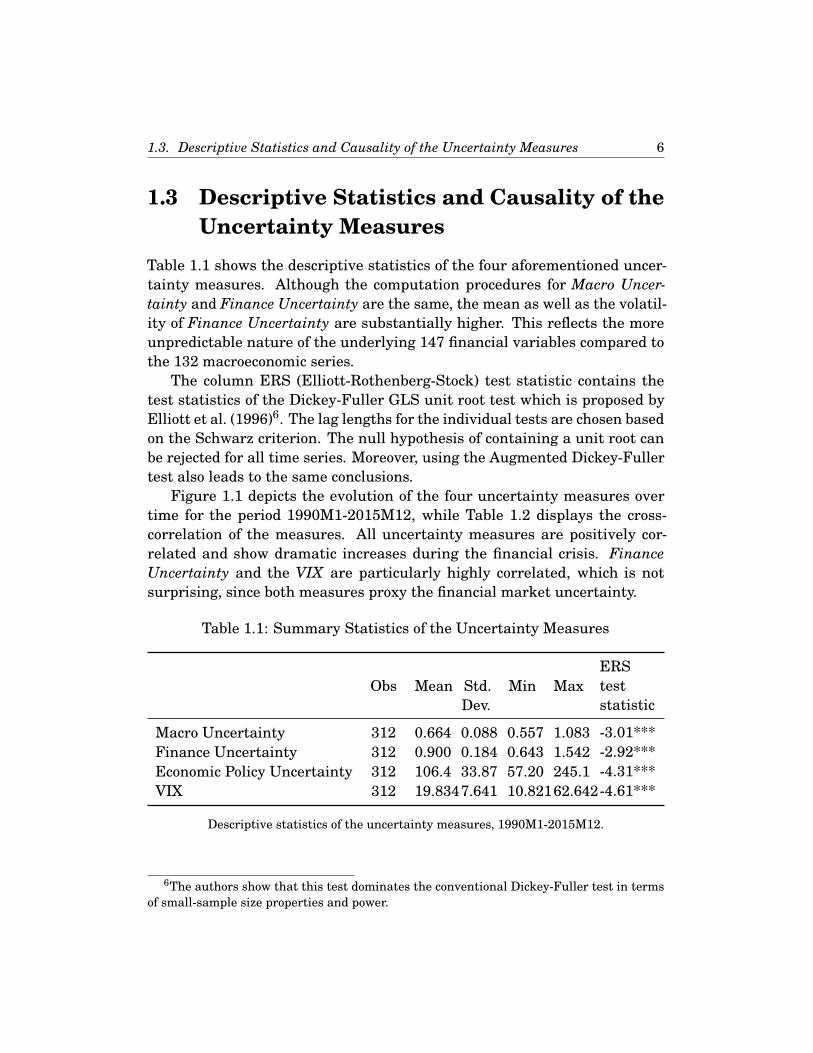
Table 1.1 shows the descriptive statistics of the four aforementioned uncer-tainty measures. Although the computation procedures for Macro Uncer-tainty and Finance Uncertainty are the same, the mean as well as the volatil-ity of Finance Uncertainty are substantially higher. This reflects the moreunpredictable nature of the underlying 147 financial variables compared tothe 132 macroeconomic series.
The column ERS (Elliott-Rothenberg-Stock) test statistic contains thetest statistics of the Dickey-Fuller GLS unit root test which is proposed byElliott et al. (1996)6. The lag lengths for the individual tests are chosen basedon the Schwarz criterion. The null hypothesis of containing a unit root canbe rejected for all time series. Moreover, using the Augmented Dickey-Fullertest also leads to the same conclusions.
Figure 1.1 depicts the evolution of the four uncertainty measures overtime for the period 1990M1-2015M12, while Table 1.2 displays the cross-correlation of the measures. All uncertainty measures are positively cor-related and show dramatic increases during the financial crisis. FinanceUncertainty and the VIX are particularly highly correlated, which is notsurprising, since both measures proxy the financial market uncertainty.
Table 1.1: Summary Statistics of the Uncertainty Measures
Obs Mean Std.Dev.
Min MaxERSteststatistic
Macro Uncertainty 312 0.664 0.088 0.557 1.083 -3.01***Finance Uncertainty 312 0.900 0.184 0.643 1.542 -2.92***Economic Policy Uncertainty 312 106.4 33.87 57.20 245.1 -4.31***VIX 312 19.8347.641 10.82162.642-4.61***
Descriptive statistics of the uncertainty measures, 1990M1-2015M12.
6The authors show that this test dominates the conventional Dickey-Fuller test in termsof small-sample size properties and power.

1.3. Descriptive Statistics and Causality of the Uncertainty Measures 7
-20
24
6N
orm
aliz
ed U
ncer
tain
ty
1990m1 2000m1 2010m1date
Macro Uncertainty Policy UncertaintyFinance Uncertainty VIX
Normalized Uncertainty Measures
Figure 1.1: Development of the Uncertainty Measures,1990M1-2015M12.
Table 1.2: Correlation of Uncertainty Measures
Macro Un-certainty
FinanceUncer-tainty
Policy Un-certainty
VIX
Macro Uncertainty 1Finance Uncertainty 0.714 1Policy Uncertainty 0.352 0.381 1VIX 0.650 0.853 0.456 1
Correlation of the uncertainty measures, 1990m1-2015M12.
Table 1.3 summarizes the p-value of the Granger causality test resultsfor all uncertainty measures. For example, in order to obtain the test resultsin column (2), the following equation was estimated7:
7Two lags are recommended by the Schwarz criterion.

1.3. Descriptive Statistics and Causality of the Uncertainty Measures 8
MUt =2∑
j=1α jMUt− j +
2∑j=1
β jFUt− j +2∑
j=1δ jPUt− j +
2∑j=1
γ jV IX t− j +ut8. (1.4)
Subsequently, the null hypotheses β1 = 0&β2 = 0, δ1 = 0&δ2 = 0 and γ1 =0&γ2 = 0 were tested to determine if Finance Uncertainty, Policy Uncertaintyand the VIX are Granger causal for Macro Uncertainty, respectively. Corre-sponding estimations and tests were also performed to obtain the remainingcolumns. There is a high level of interconnectedness between the differentuncertainty proxies. First, at the 5% significance level, Macro Uncertainty issignificantly explained by all other measures of uncertainty. Second, FinanceUncertainty and the VIX significantly affect one another. Moreover, FinanceUncertainty helps to predict all remaining uncertainty proxies and, therefore,seems to be an important driver of the overall level of economic uncertainty.
Table 1.3: Granger Causality Tests
(2) MacroUncer-tainty
(3)FinanceUncer-tainty
(4) PolicyUncer-tainty
(5) VIX
Macro Uncertainty 0.365 0.800 0.380Finance Uncertainty 0.016** 0.019** 0.000***Policy Uncertainty 0.022** 0.025** 0.537VIX 0.015** 0.005*** 0.1343
Causality tests of the uncertainty measures, 1990m1-2015M12. * indicates significance at10% level, ** indicates significance at 5% level, *** indicates significance at 1% level.
8MU denotes Macro Uncertainty, FU Finance Uncertainty and PU Policy Uncertainty.
CHAPTER 2
Uncertainty, the Option to Wait and IPO IssueCycles
Abstract: This paper uses recently developed uncertainty measures to ex-amine the role of economic uncertainty in explaining the U.S. Initial PublicOffering (IPO) issue cycles. Time series estimations reveal a strong androbust negative impact of macroeconomic and financial uncertainty on theIPO activity. For instance, an increase in macroeconomic uncertainty by onestandard deviation lowers the number of monthly IPOs by roughly four inthe long-run, which equals 20% of the average number of monthly IPOs. Inresponse to an uncertainty shock, both the reduction of the number of IPOfilings and the rise of withdrawn IPOs contribute to the lower number ofIPOs. These results support the view that firms value the option to waitand tend not to go public during periods of high uncertainty, which is akinto the occurrence of the real options effect in periods of high uncertainty ifinvestments are irreversible. However, there is no significant impact of eco-nomic policy uncertainty on the IPO market. The study also finds that highuncertainty worsens the IPO market condition by depressing stock prices,output, investor optimism and consumer sentiment.
9
2.1. Introduction 10
2.1 IntroductionThe cyclical nature of the number of initial public offerings (IPO number)is a highly debated phenomenon. Ibbotson and Jaffe (1975) and Ibbotsonet al. (1988, 1994) highlight the substantial fluctuation of new IPO issuesand more recent studies provide numerous explanations for the hot and coldIPO markets. Notably, the comprehensive empirical studies of Lowry (2003)and Ivanov and Lewis (2008) identify economic growth, stock market return,investor optimism and consumer sentiment as the most important determi-nants of IPO number. This paper provides an alternative view and arguesthat uncertainty surrounding the overall economy is also a key driver of IPOissue cycles.
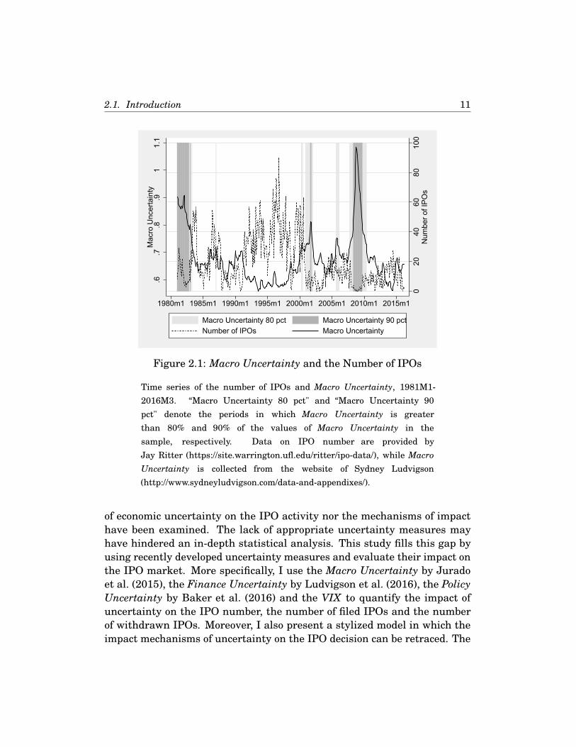
Figure 2.1 shows the evolution of IPO number and the macroeconomicuncertainty (Macro Uncertainty) measure by Jurado et al. (2015) for theperiod 1981M1-2016M3: there is a negative correlation of -0.43 between thetwo series and both variables exhibit pronounced cycles. If macroeconomicuncertainty is very high and exceeds for example its 80-th percentile1, thehigh level of uncertainty lasts for a considerable amount of periods before itdissolves2. For instance, the macroeconomic uncertainty exceeds its 80-thpercentile for 32 consecutive months during the financial crisis (2007M10-2010M5); for 28 consecutive months between 1981M1-1983M4 and for 14consecutive months between 2000M12-2002M1. During those periods ofhigh uncertainty IPO number drops quickly.
In fact, the president of NASDAQ, Adena Friedman, also relates IPOnumber to uncertainty and states3
“It’s an uncertain environment to go public in ...”(Wall Street Journal, January 20, 2016.)4
to comment the sharp drop in the number of U.S. IPOs by 75% in the firstquarter of 2016. However, neither the statistical reliability of the impact
1Exceeding its 80-th percentile means that Macro Uncertainty is greater than 80% of thevalues of Macro Uncertainty in the sample.
2Jurado et al. (2015), Ludvigson et al. (2016) and Lee et al. (2016) have documented andextensively discussed the high persistence of uncertainty shocks.
3https://www.wsj.com/articles/nasdaqs-friedman-says-ipo-environment-still-uncertain-1453295483
4There are numerous popular press articles which relate IPO activity to uncertaintyincluding the Wall Street Journal, the Financial Times, CNBC and the Washington Post.
2.1. Introduction 11
.6.7
.8.9
11.
1M
acro
Unc
erta
inty
020
4060
8010
0N
umbe
r of I
POs
1980m1 1985m1 1990m1 1995m1 2000m1 2005m1 2010m1 2015m1
Macro Uncertainty 80 pct Macro Uncertainty 90 pctNumber of IPOs Macro Uncertainty
Figure 2.1: Macro Uncertainty and the Number of IPOs
Time series of the number of IPOs and Macro Uncertainty, 1981M1-2016M3. “Macro Uncertainty 80 pct" and “Macro Uncertainty 90pct" denote the periods in which Macro Uncertainty is greaterthan 80% and 90% of the values of Macro Uncertainty in thesample, respectively. Data on IPO number are provided byJay Ritter (https://site.warrington.ufl.edu/ritter/ipo-data/), while MacroUncertainty is collected from the website of Sydney Ludvigson(http://www.sydneyludvigson.com/data-and-appendixes/).
of economic uncertainty on the IPO activity nor the mechanisms of impacthave been examined. The lack of appropriate uncertainty measures mayhave hindered an in-depth statistical analysis. This study fills this gap byusing recently developed uncertainty measures and evaluate their impact onthe IPO market. More specifically, I use the Macro Uncertainty by Juradoet al. (2015), the Finance Uncertainty by Ludvigson et al. (2016), the PolicyUncertainty by Baker et al. (2016) and the VIX to quantify the impact ofuncertainty on the IPO number, the number of filed IPOs and the numberof withdrawn IPOs. Moreover, I also present a stylized model in which theimpact mechanisms of uncertainty on the IPO decision can be retraced. The
2.1. Introduction 12
model considers an IPO as an irreversible investment with the possibility ofdelay, and borrows from the literature on irreversibility of investment anduncertainty (e.g., Pindyck, 1991; Bloom, 2009).
Using the sample period 1990M1-2015M12 and controlling for a broad setof IPO market determinant variables, I find that a one standard deviationincrease in macroeconomic uncertainty decreases IPO number by roughlyfour, which is 20% of the average number of IPOs per month. This resultis driven by both the reduction of the number of filed IPOs and the rise ofthe number of withdrawn IPOs, and suggests that firms value the optionof waiting instead of immediately going public during periods of high uncer-tainty. Furthermore, I find that uncertainty also distresses the overall IPOmarket condition by depressing stock prices, output, investor optimism andconsumer sentiment. The results are qualitatively similar and robust for theVIX, Macro Uncertainty and Finance Uncertainty in numerous specifications.Policy Uncertainty, however, does not display a significant effect on the IPOactivity.
2.1.1 Related IPO LiteratureNumerous explanations for the hot and cold IPO markets have been proposedin the finance literature. Ritter (1991) relates IPO waves to the sentiments ofinvestors, whereas Rajan and Servaes (1997) note that more firms completeIPOs when analysts are overoptimistic. Choe et al. (1993) and Yung et al.(2008) focus on the role of adverse selection but arrive at contradicting con-clusions, since they make different assumptions about the serial dependenceof innovation. However, the results of Helwege and Liang (2004) suggest thathot markets are not driven by adverse selection costs but are more likely af-fected by greater investor optimism. Lowry and Schwert (2002), Benvenisteet al. (2003) and Alti (2005) highlight the role of information spillovers ofpioneer IPOs which facilitate the pricing of subsequent issues and thus at-tract more firms to the IPO market. Pástora and Veronesi (2005) emphasizethe importance of firms’ expectation about (aggregated) profitability in ex-plaining IPO number and Chemmanur and He (2011) argue that firms gopublic to grab market share from competitors after a productivity shock. Thecomprehensive studies of Lowry (2003) and Ivanov and Lewis (2008) testthe empirical relevance of numerous explanations and identify past initialreturns of IPOs, economic growth, stock market return, the term spread, theoptimism of investors and consumer sentiment as the most important deter-
2.1. Introduction 13
minants of IPO number. I, thefore, include theses factors as control variablesin the regression analyses.
2.1.2 The Impact Mechanism of Uncertainty on the IPODecision
Typically the literature on uncertainty distinguishes between uncertaintyand risk; risk is related to the known probability distribution over a set ofevents, whereas uncertainty is associated with peoples’ inability to forecastthe likelihood of events happening (Knight, 1921). In this context, flipping afair coin is not uncertain, since the likelihood of head or tail is known, but itis risky because there is a 50% chance to obtain head with a coin flip (Bloom,2014). The disentanglement of risk and uncertainty is certainly often notpossible with real world data. Nevertheless, it helps to clarify the differencebetween risk and uncertainty, and therefore facilitates the theoretical con-sideration of how uncertainty might affect the IPO decision in the currentsubsection. In the empirical analysis, however, I follow the literature onuncertainty and use uncertainty measures which also incorporate elementsof risk.
Economic uncertainty could impact the IPO activity through differentways. First of all, given the irreversible nature of an IPO and the optionto go public at a different point in time, high uncertainty may increase theoption value of waiting of firms which consider the timing of their IPOs. Forinstance, a firm goes public only if it expects to raise at least as much capitalas the firm is worth. However, if an uncertainty shock occurs and the firmis uncertain about how much it can expect to raise from the IPO, the firmmay delay the IPO until uncertainty subsides. In addition, Lowry (2003)finds that firms go public if the business outlook is good and their demandfor new capital to boost investment is high. If firms are uncertain about theeconomic development and thus uncertain about their own capital demandand associated new investments, they may wait and gather more informationinstead of immediately going public to raise capital for new investments. Thereasoning that firms decrease investments in periods of high uncertainty isalso supported by numerous studies (e.g., Bernanke, 1983; Pindyck, 1991;Gulen and Ion, 2015).
The rationale that firms tend not to go public in periods of high uncer-tainty is consistent with the occurrence of the real options effect due to

2.1. Introduction 14
uncertainty if investments are irreversible as described in Pindyck (1991):"There will be a value to waiting (i.e., an opportunity cost to investing todayrather than waiting for information to arrive) whenever the investment isirreversible and the net payoff from the investment evolves stochasticallyover time". In other words, when a firm makes an irreversible investmentexpenditure, it essentially gives up the possibility of waiting for new informa-tion that might affect the desirability or timing of the expenditure; it cannotdisinvest should market conditions change adversely. Going public also rep-resents a form of “irreversible investment”, since a firm typically has onlyone IPO with an associated payoff which depends on the (time-varying) mar-ket condition. The higher the uncertainty about the market conditions, themore valuable the option to wait. A comparable waiting attitude can also beobserved in the merger market as suggested by Bhagwat et al. (2016). Theyfind that a one standard deviation increase in the VIX, a proxy for financialuncertainty, is associated with a 6% drop in public merger deal activity. Sim-ilarly, Jovanovic and Rousseau (2001) highlight the value of waiting in theIPO market. In their model, however, the option to delay an IPO is valuableif waiting allows a firm to gather more information about its own productionfunction.
Figure 2.2 illustrates a stylized model of a firm’s decision about the tim-ing of its IPO and how uncertainty might affect this decision. Consider afirm with a true firm value of $100, and this firm could raise $120 (goodmarket condition) with probability of p and $80 (bad market condition) withprobability 1− p in an IPO. According to the notion of risk and uncertaintyfrom above, going public is risky in general but not uncertain. It takes oneperiod of time to prepare the IPO. For example, if in t = 0 the firm decides togo public the factual IPO takes place in t = 1. The firm decides to go publiconly if it expects to raise at least as much capital as the firm is worth. Forsimplicity, the discount rate is zero. In t = 0, if there is no uncertainty at all,the firm assigns a value to p and decides to go public if p ≥ 50%. However, ifthere is a one-period uncertainty shock in t = 0 in the spirit of Knight (1921),the firm is not able to assign a value to p and postpones the IPO decision toperiod t = 1 when the uncertainty shock subsides.
Analogously, if all IPO-interested firms are homogeneous and are all hitby the same one-period uncertainty shock in period t = 0, there will be noIPOs in t = 1. As the uncertainty shock disappears in t = 1 and p ≥ 0.5,all firms go public in t = 2. For a set of heterogeneous firms a commonuncertainty shock may still reduce the number of IPOs in the subsequent

2.1. Introduction 15
period if a fraction of those firms experience the shock similarly.
Figure 2.2: Real Option of Waiting
p is the probability to raise $120 as capital (C) in an IPO.
As suggested by Figure 2.1 and the literature on uncertainty, high uncer-tainty shocks are persistent and thus are likely to impede the IPO numberfor a considerable amount of time contributing to the creation of cold IPOmarket phases. As uncertainty eventually dissolves, IPO-interested firmsstart to go public in the same time slot, which in turn could give rise to IPOhot market phases.
Last but not least, high uncertainty could overshadow the IPO marketcondition by deteriorating the business outlook. For instance, Bloom (2009),Bansal et al. (2014) and Christiano et al. (2014) conclude that high uncer-tainty decreases output, consumption and investment5, while other studiesfind that uncertainty is negatively related to aggregated growth and assetprices (e.g., Ozoguz, 2009; Pástora and Veronesi, 2012; Segal et al., 2015). Aspointed out by Pástora and Veronesi (2005) and Pástor et al. (2009), firmstend to go public if the expected (aggregate) profitability is high. Therefore,
5Some other studies on the impact of uncertainty on the real economy are Bernanke(1983), Pindyck (1991), Caballero and Pindyck (1996), Bachmann and Bayer (2013),Caggiano et al. (2014), Dorofeenko et al. (2014) and Leduc and Liu (2016). See Bloom(2014) for a more comprehensive review of the literature on uncertainty.
2.2. Data and Econometric Specification 16
IPO-interested firms may anticipate a decline in expected profitability follow-ing an uncertainty shock and choose not to go public during periods of highuncertainty. In context of the presented stylized model, following an uncer-tainty shock a decline of the business outlook may translate to a decrease ofp and a decline of the payoffs in good and bad IPO market conditions. Boththe drop of the probability to raise capital in a good market condition and thefall of the potential payoffs make firms less willing to go public.
The rest of the paper is organized as follows. Section 2.2 describes thedata, analyses the time-series properties of the key variables and presentsthe econometric model. Section 2.3 examines the impact of uncertainty on theIPO activity. Section 2.4 investigates the effects of uncertainty on IPO mar-ket condition variables including S&P 500 return, output growth, investoroptimism and consumer sentiment. Finally, section 2.5 concludes.
2.2 Data and Econometric Specification
The sample for this study is 1990M1-2015M126 and include monthly dataon IPO activity, four different uncertainty measures and numerous controlvariables. Detailed information on the data is presented in the Appendix.
2.2.1 IPO Activity DataThe number of IPOs per month and the average, equal-weighted monthlyIPO initial returns are fetched from the Ibbotson, Sindelar and Ritter (ISR)database. The initial returns represent the mean, across all IPOs each month,of the percentage difference between a closing price within the first monthafter the IPO and the offer price. A more complete description of the construc-tion of the data is in Ibbotson et al. (1994). Data on the number of filed IPOsand the number of withdrawn IPOs are provided by NASDAQ, and cover IPOactivity on the NYSE and the NASDAQ for the period 1997M1-2015M12.
6Since the VIX and the monthly GDP data are not available for earlier periods. However,analyses with the sample 1980M1-2015M12 omitting monthly GDP deliver qualitatively thesame results for Macro Uncertainty and Finance Uncertainty.
2.2. Data and Econometric Specification 17
2.2.2 Uncertainty MeasuresFinding an appropriate uncertainty measure is a challenging task, sinceuncertainty is an amorphous concept for which no objective measure exists.This study uses four uncertainty proxies which are based on different ap-proaches to approximate the latent stochastic process of uncertainty includ-ing Macro Uncertainty (Jurado et al., 2015), Finance Uncertainty (Ludvigsonet al., 2016), Policy Uncertainty (Baker et al., 2016) and the VIX.
The Macro Uncertainty by Jurado et al. (2015) captures the predictabilityof the overall macroeconomic environment; the less predictable the macroeco-nomic variables, the higher the macroeconomic uncertainty. I decided to usethe one-month-ahead measure, since the data are at a monthly frequency.The computation of Finance Uncertainty (Ludvigson et al., 2016) followsJurado et al. (2015) but uses 147 financial variables instead of 132 macroe-conomic variables as before. The Policy Uncertainty measure by Baker etal. (2016) proxies for movements in policy-related economic uncertainty byquantifying the frequency of articles in 10 leading U.S. newspapers whichcontain certain combinations of key words on economic policy uncertainty.The VIX estimates the 30-day expected volatility of the S&P 500 index. Seesection 1.2 for a more detailed description of the four uncertainty measures.
One could argue that the presented uncertainty measures capture a mix-ture of both uncertainty and risk. However, since these measures are fre-quently applied in studies that examine the effects of (economic) uncertainty,I refrain from disentangling (Knightian) uncertainty and risk in the empiri-cal part of the current paper and refer to a broader definition of uncertaintywhich also incorporates components of risk.
According to Lowry (2003), Pástora and Veronesi (2005) and Ivanov andLewis (2008), firms consider the condition of both the real economy and thefinancial market before they go public. Macro Uncertainty, which also in-corporates uncertainty components of 25 financial variables, may thereforebe the most potent uncertainty measure to explain the IPO activity, since itincorporates uncertainty about the real economy and the financial market.
2.2.3 Descriptive StatisticsTable 2.1 displays descriptive statistics of the IPO activity variables and themeasures of uncertainty. There is substantial variation of the IPO number aswell as of the number of filed IPOs. The number of withdrawn IPOs reached
2.2. Data and Econometric Specification 18
its all time high of 40 in March 2001, in a period in which Macro Uncertaintyexceeds its 90th percentile. Although the computation procedures for MacroUncertainty and Finance Uncertainty are the same, the mean as well as thevolatility of Finance Uncertainty are substantially higher. This reflects themore unpredictable nature of the underlying 147 financial variables used forthe computation of Finance Uncertainty compared to the 132 macroeconomicseries7 which underlie the computation of Macro Uncertainty.
The column ERS (Elliott-Rothenberg-Stock) test statistic contains thetest statistics of the Dickey-Fuller GLS unit root test which is proposed byElliott et al. (1996)8. The lag length for the individual tests are chosen withrespect to the Schwarz criterion. The null hypothesis of containing a unit rootcan be rejected for all time series. Using the Augmented Dickey-Fuller testleads to the same conclusions. The finding that IPO number is stationary isvery much in line with Ivanov and Lewis (2008) who also use monthly data.
The cross-correlation of the uncertainty measures and the IPO numberare presented in Table 2.2. Although the different uncertainty measures maycapture different aspects of economic uncertainty, they are highly positivelycorrelated indicating common sources of uncertainty or/and spillover effectsof one type of uncertainty on another. Finance Uncertainty and the VIXexhibit a notably high correlation of 0.85, which is not surprising, since theVIX also proxies uncertainty surrounding the financial market. Moreover,all uncertainty measures are strongly negatively correlated with the numberof initial public offerings suggesting an inverse relation between uncertaintyand IPO activity.
7The 132 macroeconomic variables already contain 25 of financial indicators.8The authors show that this test dominates the conventional Dickey-Fuller test in terms
of small-sample size properties and power.

2.2. Data and Econometric Specification 19
Table 2.1: Summary Statistics of IPO Activity Variables and UncertaintyMeasures
Obs Mean Std.Dev.
Min MaxERS teststatistic
Number of IPOs (IPO number) 312 19.669 17.562 0 100 -2.21**Number of filed IPOs 228 36.236 19.824 5 128 -3.03***Number of withdrawn IPOs 228 8.820 6.896 0 40 -6.84***Macro Uncertainty 312 0.664 0.088 0.557 1.083 -3.01***Finance Uncertainty 312 0.900 0.184 0.643 1.542 -2.92***Policy Uncertainty 312 106.43 33.87 57.20 245.12 -4.3***VIX 312 19.834 7.641 10.821 62.642 -4.61***
Sample statistics on IPO number, Macro uncertainty, Finance uncertainty, Policy uncertaintyand VIX for the period 1990M1-2015M12. Sample statistics on the number of filed IPOsand the number of withdrawn IPOs for the period 1997M1-2015M12. Data on the number offiled IPOs and the number of withdrawn IPOs are provided by NASDAQ. ERS test statisticdenotes the test statistics of the Dickey-Fuller GLS unit root test proposed by Elliott etal. (1996). The null hypothesis of containing a unit root can be rejected for all time seriesvariables. * indicates significance at 10% level, ** indicates significance at 5% level, ***indicates significance at 1% level.
Table 2.2: Correlation of IPO Number and the Uncertainty Measures
Numberof IPOs
MacroUncer-tainty
FinanceUncer-tainty
PolicyUncer-tainty
VIX
Number of IPOs 1Macro Uncertainty -0.508 1Finance Uncertainty -0.312 0.714 1Policy Uncertainty -0.477 0.352 0.381 1VIX -0.327 0.649 0.852 0.456 1
Correlation of the IPO number and uncertainty measures, 1990M1-2015M12.
2.2. Data and Econometric Specification 20
2.2.4 Control Variables in EstimationsThe results of Lowry (2003) and Ivanov and Lewis (2008) suggest that thebusiness condition, the investor and the consumer sentiments are the mostimportant drivers of IPO cycles9. Demand for capital should be higher whenbusiness conditions are more promising. For example, firms have higherdemand for capital in order to make (new) investments in times of economicgrowth, and if the financing costs from traditional bank loans are too high,the firms may raise money from the public. Moreover, companies are morelikely to go public if investors are overoptimistic and willing to pay morefor those companies than they are worth. For example, Lee et al. (1991)and Rajan and Servaes (1997) find that investor sentiment affect the IPOactivity over time. Additionally, Lowry and Schwert (2002) find a robust andsignificant impact of past average initial returns on the IPO number. Thisrelationship is attributed to the information learned during the registrationperiod. In particular, they argue that more companies file IPOs followingperiods of high initial returns because the high returns are linked to positiveinformation learned during the registration periods, indicating that compa-nies can raise more money in an IPO than they had previously thought.
Accounting for the findings of the literature, I include the S&P 500 return,the real GDP growth, the real industrial production growth, the term struc-ture, the average initial return, the investor sentiment and the consumersentiment as control variables.
2.2.5 Econometric SpecificationGiven the stationarity of the IPO activity variables and the uncertainty mea-sures, the following econometric model is estimated:
IPONumber t =β0 +k∑
i=1αi IPONumber t−i +
k∑i=1
βiUncertaintyt−i +k∑
i=1Xt−iδi +ut,
(2.1)
where IPONumber is the number of IPOs, Uncertainty denotes thechosen uncertainty measure, Xt−i is a vector containing the aforementionedcontrol variables in t− i and δi is the corresponding coefficient vector.
9See Lowry (2003) for further discussions of how the business condition and investorsentiment affect the number of firms going public.
2.3. Uncertainty and IPO Activity 21
In order to guard against endogeneity issues, all explanatory variablesare lagged. I include the first three lags of all explanatory variables in thebenchmark specification. Three lags are a conservative choice, since a largeset of explanatory variables are included. Using monthly data, Lowry andSchwert (2002) include three lags in a model with two explanatory variables,while Ivanov and Lewis (2008) use up to two lags. In specifications withtwo or one lag(s) the impact of the uncertainty measures are even moresignificant10.
I present the long-run effects of each variable in the estimation resultssection to ease interpretation11. For example, instead of presenting everyindividual βi coefficient of the impact of uncertainty, I present the long-runimpact of uncertainty
∑3i=1 βi and the corresponding standard error.
2.3 Uncertainty and IPO ActivityThis section investigates the impact of economic uncertainty on IPO activity.Throughout the remainder of the paper, Newey-West standard errors (Neweyand West, 1987) are used in order to account for possible heteroskedasticityand autocorrelation of the error term. I decided to use Macro Uncertainty asthe measure in the benchmark specification, since it quantifies the overallmacroeconomic uncertainty including uncertainty about financial and realvariables. Note that the initial return is missing in months when no IPOsoccur.
2.3.1 The Impact of Uncertainty on the Number of IPOsTable 2.3 displays the impact of Macro Uncertainty on the number of IPOsper month controlling for a large set of variables. Column (1) representsthe benchmark specification with Macro Uncertainty as uncertainty measureand all control variables included, while the other columns present alterna-tive specifications. Macro Uncertainty significantly impedes IPO numberthroughout specifications and its impact magnitude also remains moderatelyconstant. A standard deviation increase in Macro Uncertainty lowers the
10The results are presented in the Appendix.11Presenting estimations of a large set of explanatory variables with there corresponding
first three lags in one table may be confusing and impedes readability.
2.3. Uncertainty and IPO Activity 22
number of IPOs on average by roughly four IPOs12. Moreover, specificationswith Macro Uncertainty always dominate corresponding specifications with-out it in terms of explanatory power as suggested by the adjusted R, theAkaike criterion and the Schwarz criterion.
Column (2) presents the estimation results for a specification withoutMacro Uncertainty. Naturally, the adjusted R falls and the Akaike criterionand the Schwarz criterion rise in this specification compared to column (1),which indicates that Macro Uncertainty has a very high explanatory power.In absence of Macro Uncertainty in column (2), the consumer sentiment gainsmore explanatory power and its long-run coefficient and t-statistic increase,so that its impact even becomes significant at the 10% significance level. Thisresult indicates a notable dependence between Macro Uncertainty and theconsumer sentiment and suggests that the explanatory power of consumersentiment is based on its considerable correlation with Macro Uncertainty;the correlation is -0.44.
There is also a significant autoregressive component in the IPO numberitself. Alti (2005) provides a possible explanation for this finding. He arguesthat the outcomes of pioneers’ IPOs contain private information on commonvaluation factors of investors. This facilitates the pricing of subsequent is-sues and attracts more firms to go public soon after. The level of initialreturn also has a significant impact on the number of IPOs in the benchmarkspecification. Lowry and Schwert (2002) attribute this relationship to the in-formation learned during the registration period. Moreover, S&P 500 returnsshow a significant impact on the IPO number, which reflects that the numberof IPOs increases if the financial market returns are higher. In summary, thesignificant impact of the control variables are very much in line with Lowryand Schwert (2002), Lowry (2003) and Ivanov and Lewis (2008).
To compare the impact of Macro Uncertainty with those of the other uncer-tainty measures, Table 2.4 displays the impact of each uncertainty measureon the number of IPOs in the benchmark specification with all control vari-ables. Both financial market uncertainty indicators Finance Uncertaintyand the VIX have statistically significant adverse effects on the number ofIPOs. In economic terms, a one standard deviation increase in Finance Uncer-tainty and the VIX decrease the number of IPOs on average in the long-run
12(∑3
i=1 βi,MacroUncertainty) ∗ σMacroUncertainty = −39.7 ∗ 0.088 ≈ 3.5, whereσMacroUncertainty is the standard deviation of Macro Uncertainty

2.3. Uncertainty and IPO Activity 23
Table 2.3: Time Series Analysis of IPO Number
Explanatory Variables (1) (2) (3) (4) (5) (6)
Macro Uncertainty -39.7*** -41.1*** -44.4***(12.83) (11.91) (12.90)
Control variablesIPO number .7730*** .7634*** .7774*** .8261*** .7797*** .8670***
(.0578) (.0624) (.0611) (.0613) (.0591) (.0542)Underpricing .0676** .0394 .0734* .0509 .0794* .0657
(.0326) (.0496) (.0417) (.0472) (.0463) (.0488)Term structure .0095 .3848 -.149 .5127 -.294 .4756
(.6255) (.6684) (.5426) (.6411) (.5850) (.5898)SP 500 return 70.95* 85.78* 56.75* 101.0**
(39.88) (44.46) (31.71) (43.10)Industrial production growth 88.70 443.9* 79.83 311.3
(246.1) (247.6) (241.1) (242.0)GDP growth -400. -249. -400. -287.
(295.7) (281.4) (275.3) (282.3)Consumer sentiment .0426 .1616* -.047 .0189
(.1002) (.0948) (.0830) (.0803)Investor sentiment -3.31 -7.71 4.643 3.478
(8.119) (8.332) (6.545) (6.704)N 257 257 257 257 279 279Adjusted R .6647 .6192 .6699 .6427 .6616 .6371Akaike Criterion 4.776 4.889 4.740 4.829 4.716 4.776Schwarz Criterion 5.163 5.221 5.044 5.175 4.950 4.971
The table shows regressions in which the number of IPOs is the dependent variable. Robuststandard errors are in brackets. * indicates significance at 10% level, ** indicates signifi-cance at 5% level, *** indicates significance at 1% level. The sample is 1992M1-2015M12,since the monthly GDP variables are not available prior to 1992. Regressions with a sample1990M1-2015M12 without GDP growth deliver very similar results.
by roughly three and three, respectively13. This result is intuitive, since afirm wants to raise as much public capital as possible in an IPO and highfinancial market uncertainty is likely to depress investors’ willingness toinvest. The impact of Policy Uncertainty is, however, only significant at the10% significance level and the estimation with Policy Uncertainty shows thelowest explanatory power as indicated by the Adjusted R, Akaike criterionand Schwarz criterion. In contrast, Macro Uncertainty contains the high-est explanatory power which supports the view that firms take into accountthe uncertainty from the real economy and the financial market when they
13Finance Uncertainty: (∑3
i=1 βi,FinanceUncertainty)∗ σFinanceUncertainty = 15.01∗0.184 ≈2.76. VIX: (
∑3i=1 βi,V IX )∗ σV IX = 0.447∗7.641≈ 3.41.

2.3. Uncertainty and IPO Activity 24
consider an IPO. The finding that Macro Uncertainty is the most importantuncertainty driver of IPO activity is further supported by Table 2.5, whichshows the estimation results of a specification in which all control variablesand all uncertainty measures are included. In this specification, only themacroeconomic uncertainty measure displays a significant negative impacton the IPO number.
Given the robust negative impact of uncertainty on the IPO number, apersistent and high uncertainty shock could impede the IPO activity for a con-siderable amount of periods. As high uncertainty disappears IPO-interestedfirms, who valued the option to wait during periods of high uncertainty, startto go public in the same time slot. The empirical results strongly supportthe view that time-varying uncertainty is an important driver of IPO issuecycles.
Table 2.4: The Individual Impact of Different Uncertainty Measures on IPONumber
Uncertainty measure Impact onIPO
number
N AdjustedR
AkaikeCriterion
SchwarzCriterion
Macro Uncertainty -39.7*** 257 .6647868 4.776425 5.163095(12.838)
Finance Uncertainty -15.01*** 257 .6532018 4.810401 5.197072(4.9390)
Policy Uncertainty -.0418* 257 .6419197 4.842416 5.229085(.02294)
VIX -.4469*** 257 .6536126 4.809216 5.195886(.14168)
The table shows the individual impact of the different uncertainty measures on the num-ber of IPOs. The control variables in all estimations are the first three lags of S&P 500return, GDP growth, industrial production growth, term structure, consumer sentimentand investor sentiment. Robust standard errors are in brackets. * indicates significanceat 10% level, ** indicates significance at 5% level, *** indicates significance at 1% level.The sample is 1992M1-2015M12, since the monthly GDP variables are not available priorto 1992. Regressions with a sample 1990M1-2015M12 without GDP growth deliver verysimilar results.

2.3. Uncertainty and IPO Activity 25
Table 2.5: The Simultaneous Impact of Different Uncertainty Measures onIPO Number
Uncertainty measure Impact on IPO number
Macro Uncertainty -45.17**(18.461)
Finance Uncertainty 1.9730(11.082)
Policy Uncertainty -.0490(.04182)
VIX -.1588(.29643)
N 257Adjusted R .66656Akaike Criterion 4.8008Schwarz Criterion 5.3118
The table shows the impact of the different uncertainty measures on the number of IPOs in amodel where all uncertainty measures and control variables are included . The control vari-ables in all estimations are the first three lags of S&P 500 return, GDP growth, industrialproduction growth, term structure, consumer sentiment and investor sentiment. Robuststandard errors are in brackets. * indicates significance at 10% level, ** indicates signifi-cance at 5% level, *** indicates significance at 1% level. The sample is 1992M1-2015M12,since the monthly GDP variables are not available prior to 1992. Regressions with a sample1990M1-2015M12 without GDP growth deliver very similar results.
2.3.2 The Impact of Uncertainty on the IPO TimingIn general, companies and/or underwriters have three ways to influence thetiming of an IPO. First, companies can choose the time to file the issue.Second, the planned issue date can be changed. Third, they can withdrawthe issue. The strong negative relationship between uncertainty and thesubsequent number of IPOs indicate that firms time their IPOs in responseto the level of uncertainty. This subsection sheds light on the IPO timing offirms and investigates the relation between uncertainty and the number ofIPO filings and the number of withdrawn IPOs.
Table 2.6 presents the estimation results for the number of filed and the

2.3. Uncertainty and IPO Activity 26
number of withdrawn IPOs which are explained by different uncertaintymeasures, controlling for the whole available set of control variables fromEquation (2.1). In other words, the IPONumber from Equation (2.1) is re-placed by the number of filed and the number of withdrawn IPOs, respectively.Here, the number of withdrawn IPOs are weighted by the sum of the numberof filed IPOs in the four previous months. This weighting approach is analo-gous to Lowry and Schwert (2002) and scales the number of withdrawn IPOsby the number of firms which could have possibly withdrawn their IPOs14.However, no weighting or weighting with less than four months lead to thesame qualitative conclusion. I include the first two lags of all explanatoryvariables, considering the smaller sample size and the recommendation ofthe Schwarz criterion.
All uncertainty measures have significant negative impact on the IPOtiming, except for Policy Uncertainty. The insignificance of Policy Uncer-tainty is expected, since Policy Uncertainty does not impact the IPO numbersignificantly in the analysis of the previous subsection. An increase in un-certainty leads to a lower number of firms who file an IPO and raises thenumber of withdrawn IPOs. The latter is particularly notable, since with-drawing an IPO has numerous associated costs. First, withdrawing an IPOmay delay profitable investment due to financing shortage. This cost is par-ticularly high for firms in nascent industries in which an early entranceensures first-mover advantages. A second cost of withdrawing an IPO is theincreased uncertainty about the firm valuation and an associated bad repu-tation, which may hinder raising capital from the public securities marketsin the future. Lerner (1994) argues that even if the stated reason for the IPOwithdrawal is poor market conditions, the firm may still be lumped with othercompanies whose offerings did not sell because of questionable accountingpractices or gross overpricing. In the same vein, Dunbar and Foerster (2008)discover that only about 9% of withdrawn IPOs are able to return to have asuccessful IPO and Lian and Wang (2009) find that the negative connotationsof the first-time withdrawal translate into lower valuations for second-timeIPOs. Therefore, high uncertainty seems to be of significant importance tothe firms, so that they withdraw their IPO in response to an uncertaintyshock despite the potential withdrawal costs.
14By using the scaled number of withdrawn IPOs in the regression, the magnitude ofimpact cannot be easily calculated. However, the sign and significance of impact can still beinterpreted straightforwardly: A positive and significant coefficient of uncertainty indicatesthat an increase in uncertainty leads to an increase in withdrawn IPOs on average.
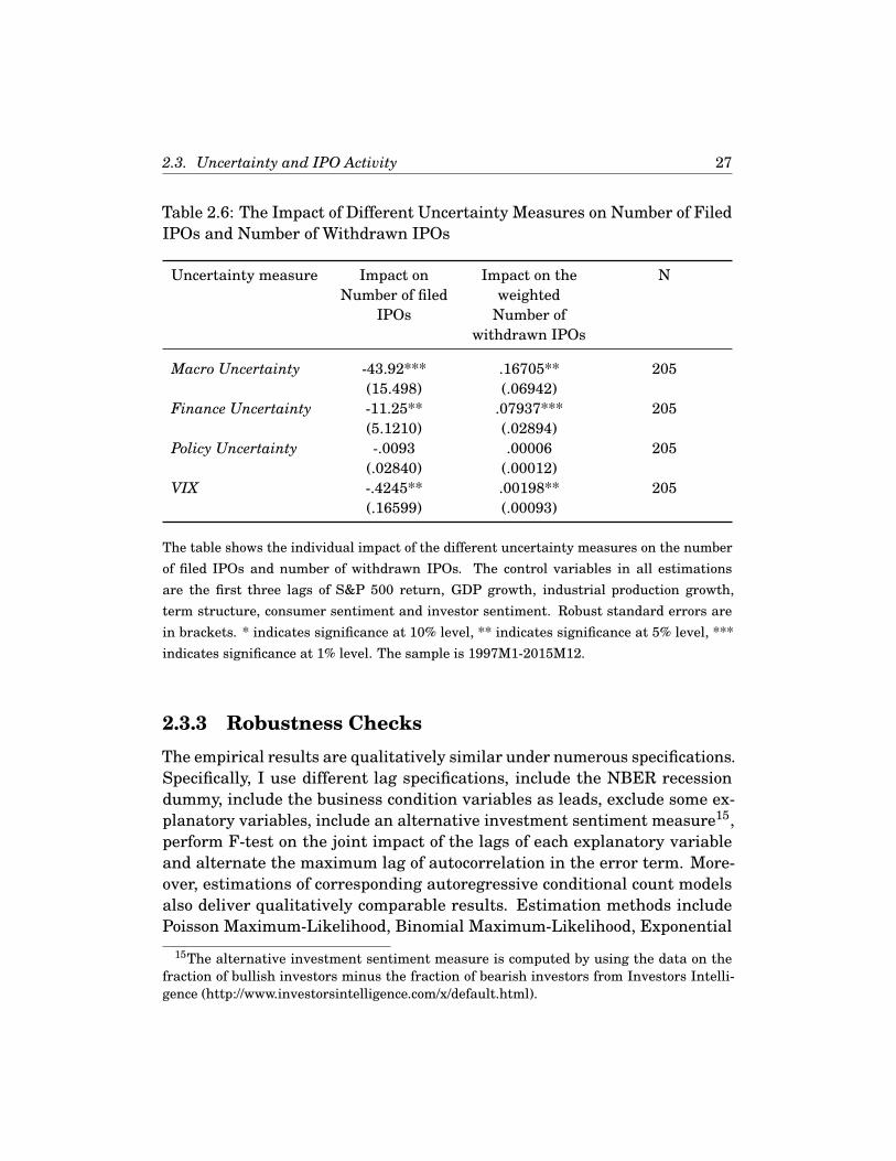
2.3. Uncertainty and IPO Activity 27
Table 2.6: The Impact of Different Uncertainty Measures on Number of FiledIPOs and Number of Withdrawn IPOs
Uncertainty measure Impact onNumber of filed
IPOs
Impact on theweighted
Number ofwithdrawn IPOs
N
Macro Uncertainty -43.92*** .16705** 205(15.498) (.06942)
Finance Uncertainty -11.25** .07937*** 205(5.1210) (.02894)
Policy Uncertainty -.0093 .00006 205(.02840) (.00012)
VIX -.4245** .00198** 205(.16599) (.00093)
The table shows the individual impact of the different uncertainty measures on the numberof filed IPOs and number of withdrawn IPOs. The control variables in all estimationsare the first three lags of S&P 500 return, GDP growth, industrial production growth,term structure, consumer sentiment and investor sentiment. Robust standard errors arein brackets. * indicates significance at 10% level, ** indicates significance at 5% level, ***indicates significance at 1% level. The sample is 1997M1-2015M12.
2.3.3 Robustness ChecksThe empirical results are qualitatively similar under numerous specifications.Specifically, I use different lag specifications, include the NBER recessiondummy, include the business condition variables as leads, exclude some ex-planatory variables, include an alternative investment sentiment measure15,perform F-test on the joint impact of the lags of each explanatory variableand alternate the maximum lag of autocorrelation in the error term. More-over, estimations of corresponding autoregressive conditional count modelsalso deliver qualitatively comparable results. Estimation methods includePoisson Maximum-Likelihood, Binomial Maximum-Likelihood, Exponential
15The alternative investment sentiment measure is computed by using the data on thefraction of bullish investors minus the fraction of bearish investors from Investors Intelli-gence (http://www.investorsintelligence.com/x/default.html).
2.4. Uncertainty and the IPO Market Conditions 28
Quasi-Maximum-Likelihood and Normal Quasi-Maximum-Likelihood. Lastbut not least, I estimate the impact of Macro Uncertainty and Finance Uncer-tainty with the sample 1981M1-2015M12 without monthly GDP as controlvariable and obtain similar results16.
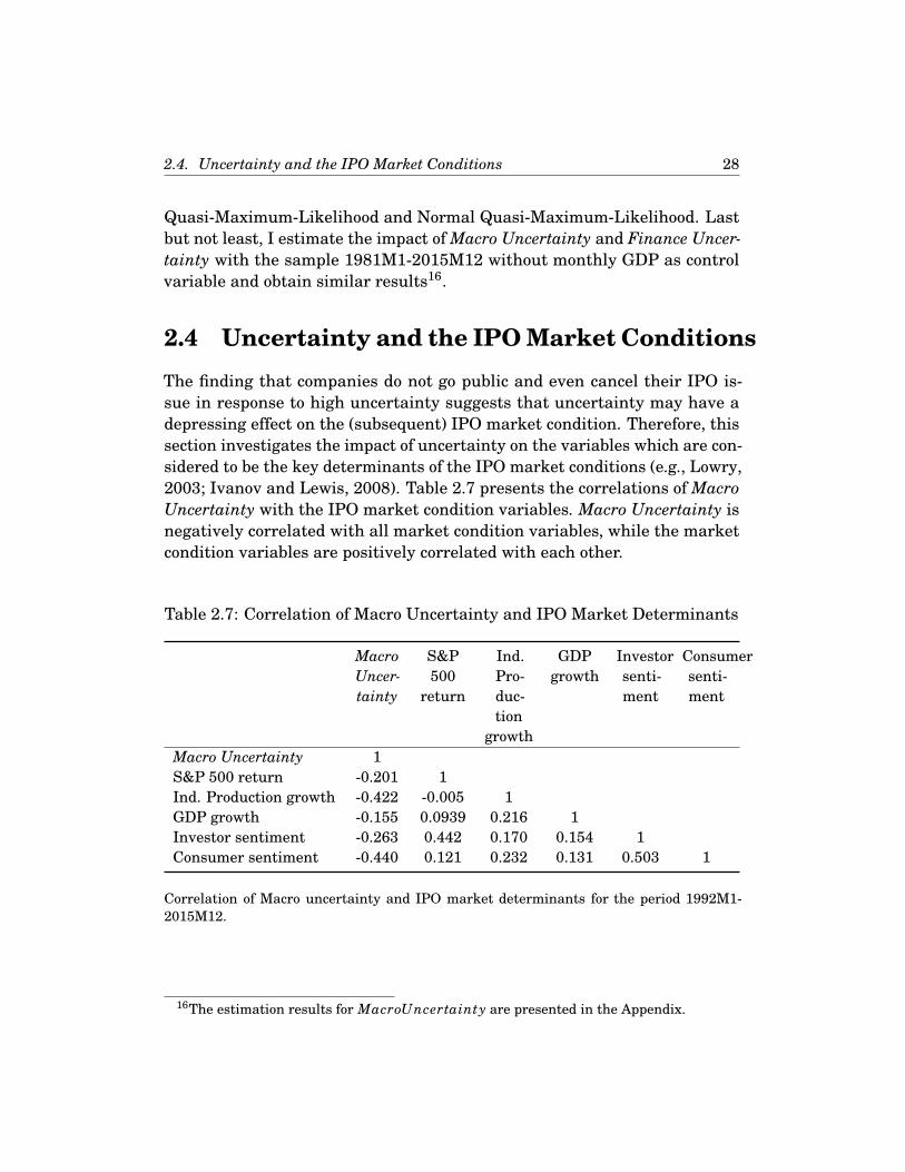
2.4 Uncertainty and the IPO Market ConditionsThe finding that companies do not go public and even cancel their IPO is-sue in response to high uncertainty suggests that uncertainty may have adepressing effect on the (subsequent) IPO market condition. Therefore, thissection investigates the impact of uncertainty on the variables which are con-sidered to be the key determinants of the IPO market conditions (e.g., Lowry,2003; Ivanov and Lewis, 2008). Table 2.7 presents the correlations of MacroUncertainty with the IPO market condition variables. Macro Uncertainty isnegatively correlated with all market condition variables, while the marketcondition variables are positively correlated with each other.
Table 2.7: Correlation of Macro Uncertainty and IPO Market Determinants
MacroUncer-tainty
S&P500
return
Ind.Pro-duc-tion
growth
GDPgrowth
Investorsenti-ment
Consumersenti-ment
Macro Uncertainty 1S&P 500 return -0.201 1Ind. Production growth -0.422 -0.005 1GDP growth -0.155 0.0939 0.216 1Investor sentiment -0.263 0.442 0.170 0.154 1Consumer sentiment -0.440 0.121 0.232 0.131 0.503 1
Correlation of Macro uncertainty and IPO market determinants for the period 1992M1-2015M12.
16The estimation results for MacroUncertainty are presented in the Appendix.

2.4. Uncertainty and the IPO Market Conditions 29
For each of the key variables (S&P 500 return, industrial productiongrowth, GDP growth, investor and consumer sentiment) the following regres-sion equation is estimated:
yt =β0 +k∑
i=1αi yt−i +
k∑i=1
βiUncertaintyt−i +k∑
i=1Xt−iδi +ut, (2.2)
where y denotes a key variable, Uncertainty the uncertainty measure andXt−i the vector of control variables which contains the remaining key vari-ables in t− i.
Table 2.8 summarizes the (long-run) impact of the different measuresof uncertainty on the IPO market determinants. In the third column theimpact of the uncertainty measures on the stock market return is presented.Macro Uncertainty and Finance Uncertainty adversely affect the S&P 500returns. This result is consistent with Segal et al. (2015), who find that uncer-tainty, which is associated with negative innovation, decreases asset prices.Industrial production is negatively affected by a rise in Macro Uncertainty,Finance Uncertainty and the VIX. Bloom (2009) also finds that an increaseof the VIX leads to a drop in output. However, GDP growth and investorsentiment are only significantly affected by Macro Uncertainty, while onlyPolicy Uncertainty has a significant impact on consumer sentiment.
The different uncertainty measures capture different aspects of economicuncertainty and therefore have different impacts on the economic and senti-ment variables. Among them Macro Uncertainty is the strongest predictorof the IPO market determinants. In fact, Macro Uncertainty also performsbest in explaining IPO activity in section 2.3 in terms of significance and ex-planatory power. These results strongly encourage the reasoning that firmsconsider the uncertainty of real and financial variables when they plan to gopublic.

2.5. Conclusion 30
Table 2.8: The Impact of Different Uncertainty Measures on IPO MarketDeterminants
Uncertainty Measure N S&P 500return
Ind.production
growth
GDPgrowth
Investorsentiment
Consumersentiment
Macro Uncertainty 285 -.113*** -.028*** -.009** -.150** -2.868(.04061) (.01050) (.00457) (.07604) (2.4304)
Finance Uncertainty 285 -.033** -.007** -.0025 -.0163 .03928(.01557) (.00310) (.00176) (.03391) (1.0204)
Policy Uncertainty 285 .00014 0.000 0.000 .00024 -.019**(.00009) (.00002) (.00001) (.00024) (.00963)
VIX 285 .00011 -.00017** -.0000 .00030 .03649(.00041) (.00008) (.00004) (.00077) (.02307)
The table shows the individual impact of the different uncertainty measures on the businesscondition and sentiment variables. The control variables in all estimations are the lagsof S&P 500 return, GDP growth, industrial production growth, consumer sentiment andinvestor sentiment. Robust standard errors are in brackets. * indicates significance at 10%level, ** indicates significance at 5% level, *** indicates significance at 1% level. The sampleis 1992M1-2015M12.
2.5 ConclusionDespite the large literature on IPO, we still have relatively little understand-ing of why IPO hot and cold market phases exist. I provide an alternativeexplanation for the occurrence of IPO issue cycles by relating these cycles totime-varying economic uncertainty. Specifically, I empirically analyze the im-pact of recently developed measures of economic uncertainty on the numberof IPOs, the number of newly filed IPOs and the number of withdrawn IPOs.The estimations reveal a robust and negative impact of uncertainty on IPOactivity. For example, a one standard deviation increase in macroeconomicuncertainty decreases the number of IPOs by roughly four. Both the reduc-tion of the number of newly filed IPOs and the increase of the number ofwithdrawn IPOs contribute to the lower IPO number. These findings suggestthe existence of the real options effect of waiting in the IPO market duringperiods of high uncertainty. Moreover, I find that an increase in uncertaintyis negatively related to the (future) IPO market condition variables whichinclude the S&P 500 return, GDP growth, industrial production growth, in-vestor optimism and consumer sentiment. The empirical results also identify
2.5. Conclusion 31
macroeconomic uncertainty as the most crucial uncertainty driver of theIPO market. Since high uncertainty shocks are relatively persistent andtake some time to fade away, they are likely to impede the IPO number fora considerable amount of periods, and as uncertainty eventually dissolves,IPO-interested firms start to go public in the same time slot. This mechanismhelps to widen the understanding of why IPO issue cycles exist. Neverthe-less, it would be interesting to see if the response to uncertainty shocks hassectoral variation. For example, firms in capital-intensive industries mightbe more cautious than IT-firms, which are more willing to go public as soonas possible to ensure the first-mover advantage in a fast-paced market.
2.5. Conclusion 32
Appendix
Data Appendix• IPO data
– Number of IPOs (IPO number): The number of IPOs per month areprovided by Jay Ritter (https://site.warrington.ufl.edu/ritter/ipo-data/).
– Initial returns (Underpricing): The initial returns represent themean, across all IPOs each month, of the percentage differencebetween a closing price within the first month after the IPO andthe offer price. A more complete description of the construction ofthe data is in Ibbotson et al. (1994). The data is provided by JayRitter (https://site.warrington.ufl.edu/ritter/ipo-data/).
– Number of filed IPOs: The number of filed IPOs per month arefetched from the NASDAQ IPO database.
– Number of withdrawn IPOs: The number of withdrawn IPOs permonth are fetched from the NASDAQ IPO database.
• Uncertainty Measures
– Macro Uncertainty: The macroeconomic uncertainty by Jurado etal. (2015) is collected from the website of Sydney Ludvigson(http://www.sydneyludvigson.com/data-and-appendixes/)
– Finance Uncertainty: The financial uncertainty by Ludvigson etal. (2016) is collected from the website of Sydney Ludvigson(http://www.sydneyludvigson.com/data-and-appendixes/)
– Policy Uncertainty: The economic policy uncertainty by Baker etal. (2016) is collected from http://www.policyuncertainty.com/
– VIX: The VIX is collected from the Federal Reserve Bank ofSt.Louis (https://fred.stlouisfed.org).
• Other variables
– The S&P 500, the industrial production index and the consumerconfidence are collected from the Federal Reserve Bank of St.Louis(https://fred.stlouisfed.org).

2.5. Conclusion 33
– Monthly GDP: Monthly GDP is collected from the MacroeconomicAdvisers database (http://www.macroadvisers.com/).
– Term spread: Term spread is collected from the Federal ReserveBank of New York.
– Investor sentiment: I follow Han (2008) and proxy investor sen-timent as the fraction of bullish investors minus the fraction ofbearish investors. I use the database from the American Asso-ciation of Individual Investors (http://www.aaii.com/) to calculatethe investor sentiment for the benchmark estimation. As a ro-bustness check, I use the database from Investors Intelligence(http://www.investorsintelligence.com/x/default.html) to computethe investor sentiment. The overall results are very similar.

2.5. Conclusion 34
Supportive Tables
Table 2.9: Time Series Analysis of IPO Number with Two Lags
Explanatory Variables (1) (2) (3) (4) (5) (6)
Macro Uncertainty -39.5*** -43.1*** -40.7***(11.51) (11.21) (11.98)
Control variablesIPO number .7182*** .7721*** .7295*** .7721*** .7230*** .8002***
(.0564) (.0598) (.0588) (.0598) (.0592) (.0556)Underpricing .0662** .0485 .0807* .0485 .0730 .0592
(.0334) (.0503) (.0478) (.0503) (.0497) (.0507)Term structure -.004 .6909 -.364 .6909 -.134 .6902
(.5595) (.6268) (.5419) (.6268) (.5941) (.5994)SP 500 return 24.64 48.76 14.69 48.76
(24.83) (30.01) (25.50) (30.01)Industrial production growth -28.7 157.8 -42.4 157.8
(177.2) (180.3) (178.4) (180.3)GDP growth -315. -246 -299. -246
(202.4) (199.7) (192.1) (199.7)Consumer sentiment .0933 .1761** .0271 .0995
(.0851) (.0859) (.0807) (.0786)Investor sentiment -2.56 -6.87 .7796 -1.01
(6.935) (7.362) (5.713) (5.838)N 264 264 264 264 287 287Adjusted R .6347 .6206 .6386 .6206 .6343 .6173Akaike Criterion 4.821 4.852 4.796 4.852 4.763 4.802Schwarz Criterion 5.078 5.082 4.999 5.082 4.916 4.929
The table shows regressions in which the number of IPOs is the dependent variable. The firsttwo lags of all explanatory variables are included in the estimation. Robust standard errorsare in brackets. * indicates significance at 10% level, ** indicates significance at 5% level,*** indicates significance at 1% level. The sample is 1992M1-2015M12, since the monthlyGDP variables are not available prior to 1992. Regressions with a sample 1990M1-2015M12without GDP growth deliver very similar results.
2.5. Conclusion 35
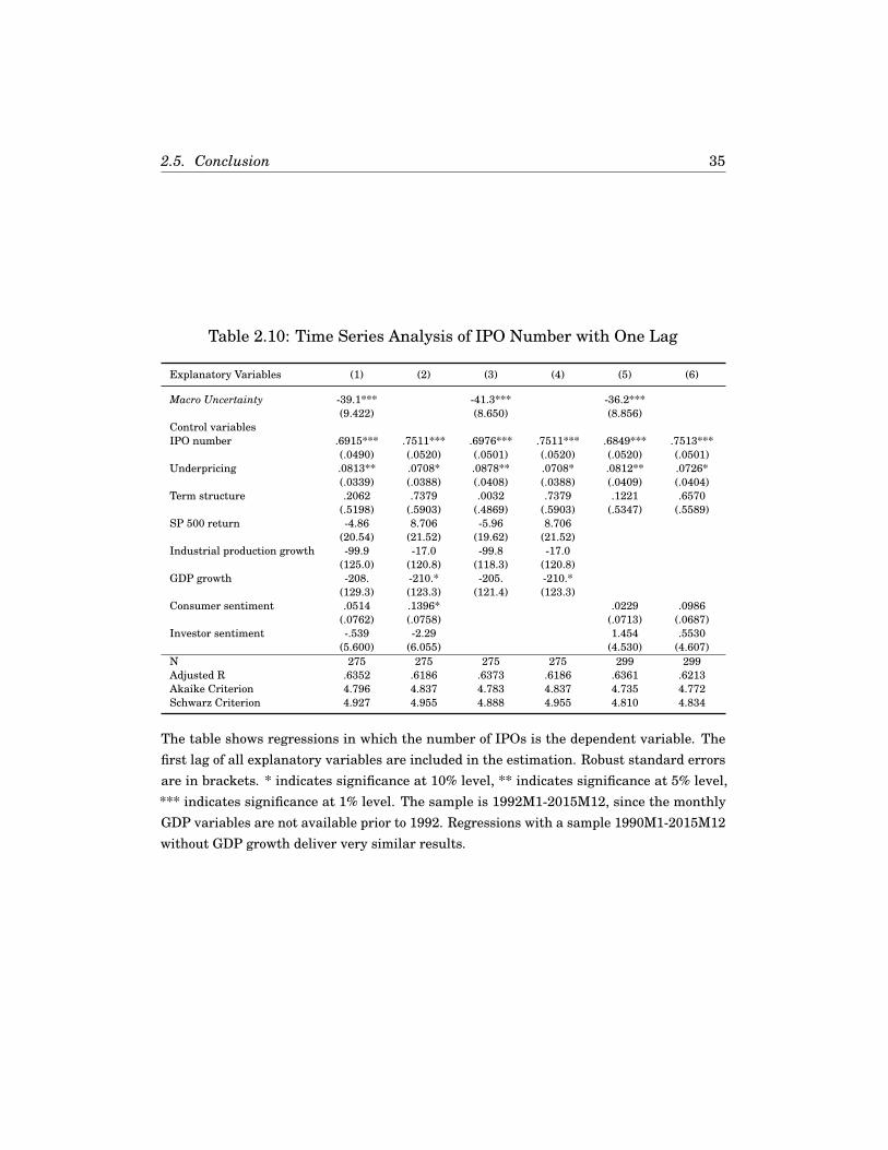
Table 2.10: Time Series Analysis of IPO Number with One Lag
Explanatory Variables (1) (2) (3) (4) (5) (6)
Macro Uncertainty -39.1*** -41.3*** -36.2***(9.422) (8.650) (8.856)
Control variablesIPO number .6915*** .7511*** .6976*** .7511*** .6849*** .7513***
(.0490) (.0520) (.0501) (.0520) (.0520) (.0501)Underpricing .0813** .0708* .0878** .0708* .0812** .0726*
(.0339) (.0388) (.0408) (.0388) (.0409) (.0404)Term structure .2062 .7379 .0032 .7379 .1221 .6570
(.5198) (.5903) (.4869) (.5903) (.5347) (.5589)SP 500 return -4.86 8.706 -5.96 8.706
(20.54) (21.52) (19.62) (21.52)Industrial production growth -99.9 -17.0 -99.8 -17.0
(125.0) (120.8) (118.3) (120.8)GDP growth -208. -210.* -205. -210.*
(129.3) (123.3) (121.4) (123.3)Consumer sentiment .0514 .1396* .0229 .0986
(.0762) (.0758) (.0713) (.0687)Investor sentiment -.539 -2.29 1.454 .5530
(5.600) (6.055) (4.530) (4.607)N 275 275 275 275 299 299Adjusted R .6352 .6186 .6373 .6186 .6361 .6213Akaike Criterion 4.796 4.837 4.783 4.837 4.735 4.772Schwarz Criterion 4.927 4.955 4.888 4.955 4.810 4.834
The table shows regressions in which the number of IPOs is the dependent variable. Thefirst lag of all explanatory variables are included in the estimation. Robust standard errorsare in brackets. * indicates significance at 10% level, ** indicates significance at 5% level,*** indicates significance at 1% level. The sample is 1992M1-2015M12, since the monthlyGDP variables are not available prior to 1992. Regressions with a sample 1990M1-2015M12without GDP growth deliver very similar results.

2.5. Conclusion 36
Table 2.11: Time Series Analysis of IPO Number without Monthly GDP
Explanatory Variables (1) (2) (3) (4) (5) (6)
Macro Uncertainty -39.3*** -39.9*** -44.4***(12.88) (12.31) (12.90)
Control variablesIPO number .7873*** .7800*** .7852*** .8449*** .7797*** .8670***
(.0549) (.0583) (.0598) (.0564) (.0591) (.0542)Underpricing .0720** .0466 .0735* .0567 .0794* .0657
(.0322) (.0510) (.0423) (.0477) (.0463) (.0488)Term structure .0577 .5691 .0124 .6412 -.294 .4756
(.5874) (.6398) (.5215) (.6113) (.5850) (.5898)SP 500 return 91.97** 112.4*** 81.08*** 126.5***
(37.27) (40.92) (28.93) (39.93)Industrial production growth -133. 195.1 -157. 85.24
(207.2) (213.8) (212.6) (206.6)Consumer sentiment .0056 .1247 -.047 .0189
(.0886) (.0873) (.0830) (.0803)Investor sentiment -1.44 -6.12 4.643 3.478
(7.487) (7.631) (6.545) (6.704)N 277 277 277 277 279 279Adjusted R .6603 .6144 .6650 .6410 .6616 .6371Akaike Criterion 4.749 4.863 4.716 4.795 4.716 4.776Schwarz Criterion 5.076 5.138 4.964 5.082 4.950 4.971
The table shows regressions in which the number of IPOs is the dependent variable. Robuststandard errors are in brackets. * indicates significance at 10% level, ** indicates signifi-cance at 5% level, *** indicates significance at 1% level. The sample is 1990M1-2015M12.
2.5. Conclusion 37
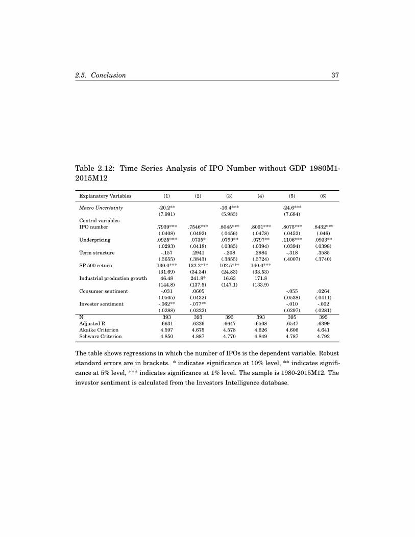
Table 2.12: Time Series Analysis of IPO Number without GDP 1980M1-2015M12
Explanatory Variables (1) (2) (3) (4) (5) (6)
Macro Uncertainty -20.2** -16.4*** -24.6***(7.991) (5.983) (7.684)
Control variablesIPO number .7939*** .7546*** .8045*** .8091*** .8075*** .8432***
(.0408) (.0492) (.0456) (.0478) (.0452) (.046)Underpricing .0925*** .0735* .0799** .0797** .1106*** .0933**
(.0293) (.0418) (.0385) (.0394) (.0394) (.0398)Term structure -.157 .2941 -.208 .2984 -.318 .3585
(.3655) (.3843) (.3855) (.3724) (.4007) (.3740)SP 500 return 130.0*** 132.2*** 102.5*** 140.0***
(31.69) (34.34) (24.83) (33.53)Industrial production growth 46.48 241.8* 16.63 171.8
(144.8) (137.5) (147.1) (133.9)Consumer sentiment -.031 .0605 -.055 .0264
(.0505) (.0432) (.0538) (.0411)Investor sentiment -.062** -.077** -.010 -.002
(.0288) (.0322) (.0297) (.0281)N 393 393 393 393 395 395Adjusted R .6631 .6326 .6647 .6508 .6547 .6399Akaike Criterion 4.597 4.675 4.578 4.626 4.606 4.641Schwarz Criterion 4.850 4.887 4.770 4.849 4.787 4.792
The table shows regressions in which the number of IPOs is the dependent variable. Robuststandard errors are in brackets. * indicates significance at 10% level, ** indicates signifi-cance at 5% level, *** indicates significance at 1% level. The sample is 1980-2015M12. Theinvestor sentiment is calculated from the Investors Intelligence database.

CHAPTER 3
Real Options Effect of Uncertainty and LaborDemand Shocks on the Housing Market
This chapter is joint work with Gabriel Lee and Johannes Strobel.
Abstract: This paper documents that macroeconomic uncertainty affectsthe housing market in two significant ways. First, uncertainty shocks ad-versely affect housing prices but not the quantities that are traded. Con-trolling for a broad set of variables in fixed-effects regressions, we find thatuncertainty shocks reduce housing prices and median sales prices in theamount of 1.4% and 1.8%, respectively, but the effect is not statistically sig-nificant for the percentage changes of all homes sold. Second, when bothuncertainty and local demand shocks are introduced, the effects of uncer-tainty on the housing market dominate that of local labor demand shocks onhousing prices, median sell prices, the share of houses selling for loss, andtransactions. The aforementioned effects are largest for the states that ex-hibit relatively high housing price volatilities, suggesting real options effectsin the housing market during the times of high uncertainty.
38

3.1. Introduction 39
3.1 IntroductionThree well documented features of the recent Great Recession are the declinein housing prices, the increase in unemployment rate, and the increase in thepresence of uncertainty in the United States. Figure 3.1 shows the correla-tion between the U.S. housing price growth rate and some of the uncertaintymeasures in the recent literature over the period from 1990 to 2014 withthe highlighted recession periods: a clear negative correlation between thehousing price growth rate and the shown uncertainty measures.1
r(House Price Growth, Macro)=-0.44r(., Policy)=-0.34r(., State)=-0.16r(., Vix)=-0.18
-30
36
Nor
mal
ized
Unc
erta
inty
-.02
0.0
2.0
4H
ouse
Pric
e G
row
th R
ates
1990m1 1994m3 1998m5 2002m7 2006m9 2010m11 2015m1date
Recession Housing Price Growth RatesNormalized Macro Normalized PolicyNormalized State Normalized Vix
House Price Growth Rates and Uncertainty Proxies
Figure 3.1: House Price Growth Rates and Uncertainty Prox-ies
Time series of the house price growth rates and the four uncertainty mea-sures, 1990M1-2014M12. The shaded areas denote the periods of reces-sion according to the NBER definition.
1We use four different uncertainty measures in our analysis: the Macro Uncertaintyby Jurado et al. (2015), the VIX by Bloom (2009), the Policy Uncertainty by Baker et al.(2016), and our measure, which is analogous to Baker et al. (2016) but on a state level (StateUncertainty). Correlations between these uncertainty measure over these periods rangebetween 0.25 and 0.63.
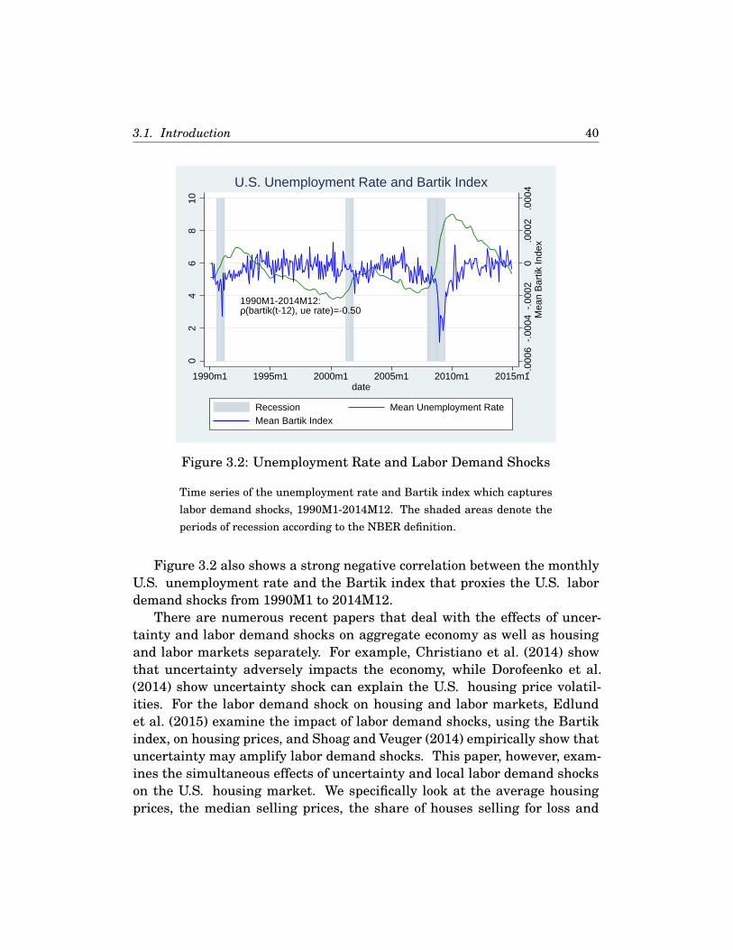
3.1. Introduction 40
1990M1-2014M12:r(bartik(t-12), ue rate)=-0.50
-.00
06-.
0004
-.00
020
.000
2.0
004
Mea
n B
artik
Inde
x
02
46
810
1990m1 1995m1 2000m1 2005m1 2010m1 2015m1date
Recession Mean Unemployment RateMean Bartik Index
U.S. Unemployment Rate and Bartik Index
Figure 3.2: Unemployment Rate and Labor Demand Shocks
Time series of the unemployment rate and Bartik index which captureslabor demand shocks, 1990M1-2014M12. The shaded areas denote theperiods of recession according to the NBER definition.
Figure 3.2 also shows a strong negative correlation between the monthlyU.S. unemployment rate and the Bartik index that proxies the U.S. labordemand shocks from 1990M1 to 2014M12.
There are numerous recent papers that deal with the effects of uncer-tainty and labor demand shocks on aggregate economy as well as housingand labor markets separately. For example, Christiano et al. (2014) showthat uncertainty adversely impacts the economy, while Dorofeenko et al.(2014) show uncertainty shock can explain the U.S. housing price volatil-ities. For the labor demand shock on housing and labor markets, Edlundet al. (2015) examine the impact of labor demand shocks, using the Bartikindex, on housing prices, and Shoag and Veuger (2014) empirically show thatuncertainty may amplify labor demand shocks. This paper, however, exam-ines the simultaneous effects of uncertainty and local labor demand shockson the U.S. housing market. We specifically look at the average housingprices, the median selling prices, the share of houses selling for loss and
3.1. Introduction 41
transactions (houses sold). More precisely, we seek to answer (i) does uncer-tainty directly affect the housing market, (ii) if a local labor demand shockoccurs in a period of high uncertainty, is the impact different compared toa period of low uncertainty and (iii) how robust are the outcomes given thechoice of the uncertainty proxy and the threshold level defining a period ofhigh uncertainty?
First, controlling for a broad set of variables, we find that uncertaintyshocks directly affect prices but not quantities. The median sell price as wellas the housing price decrease on average by 1.80% and 1.42%, respectively.Second, a positive local labor demand shock significantly increases mediansell prices, house prices and transactions and decreases the share of housesselling for loss. If a labor demand shock occurs during a period of high un-certainty, however, then it essentially affects neither prices nor quantities:Home sellers and -buyers do not trade at the price and wait out in selling andbuying until the uncertainty periods are over. This observation is consistentwith the occurrence of a real options effect akin to the irreversibility of aninvestment described by Pindyck (1991, p.1117): "There will be a value towaiting (i.e., an opportunity cost to investing today rather than waiting forinformation to arrive) whenever the investment is irreversible and the netpayoff from the investment evolves stochastically over time". For instance,Bloom et al. (2007) show that because of real options effects, firms’ respon-siveness to demand shocks is generally lower in periods of high uncertainty.Capozza and Helsley (1990) are the first to examine the impact of uncertaintyon land values and development decisions in a spatial context. Geltner etal. (1996) show that alternative uses lead to a delay in development, whileChilds et al. (1996) demonstrate that the ability to mix uses and to redevelopaffects the timing of land development. Holland et al. (2000), Childs et al.(2002), Clapp et al. (2013), Bulan et al. (2009), and Cunningham (2006, 2007)empirically show that real options play an important role for house pricesdynamics, housing investment and land prices.
Analogous to the irreversible investment literature, we find the responseof housing market variables to labor demand shocks to be much lower intimes of high uncertainty, suggesting real options effects (option to "waitand see") in the housing market during times of high uncertainty. Morespecifically, we show that following an adverse shock in labor demand of onestandard deviation, the real option value ("wait and see" effect) in the hous-ing price amounts to 0.19%, and the effect increases to 0.32% for the states(locations) that exhibit relatively high housing price volatilities. Further-

3.1. Introduction 42
more, we find that following an adverse labor demand shock, not only theshare of houses selling for loss significantly decreases in times of high uncer-tainty when compared to normal times, but also the number of homes soldremains almost constant.2 To show that the real option value increases withhigher uncertainty, we sort the fifty one states into three equal-sized groups,according to the unconditional housing price volatility in each state. In doingso, we find that while the impact of local labor demand shocks is largest forthe group with the highest housing price volatility, uncertainty completelyoffsets the labor demand shock - as opposed to the other two groups, wherewe find no significant impact of uncertainty.
Our results, thus, indicate uncertainty shocks affect housing price move-ments both directly and indirectly. On the one hand, uncertainty adverselyaffects housing prices. On the other hand, it alters the impact of shocksduring uncertain times, with this latter effect consistent with the presenceof real option effects arising in a period of high uncertainty in the housingmarket.3 One important implication of our results, analogous to Bloom et al.(2007), is that in order for policy measures to work properly, highest priorityshould be given to the reduction of uncertainty.4
We address real option issues in housing markets using monthly U.S.state-level data from 1990 to 2014. We construct binary uncertainty dum-mies to indicate the periods of high uncertainty, as in Bloom (2009) and avariation of the Bartik index proposed by Bartik (1991) as local labor demandshocks to quantify the impact of these two shocks on the housing market. Ourapproach thus corresponds to models using two-state Markov-switching pro-cesses, where regime changes can be documented by an uncertainty indexcrossing various threshold values, which are based on the percentiles of thedistribution of the uncertainty proxy. Our approach in defining the thresholdvalues differs from the one used in, for example, Bloom (2009), who definesperiods of uncertainty as the proxy when 1.65 or more standard deviationsabove the mean. We use the macroeconomic uncertainty measure by Jurado
2We show the robustness of the above results to different threshold values that are rangedfrom 80th, 85th, 90th and 95th percentile of an uncertainty proxy.
3See also Aastveit et al. (2013), in which structural Vector Autoregressions are used todocument wait-and-see effects in monetary policy during periods of high uncertainty. Seealso Bloom (2014) for further discussion and sectors where real option effects arise.
4Especially in light of the results of Stroebel and Vavra (2014), who show that there isa causal relation between changes in housing prices and changes in retails prices and thusconsumption.

3.2. Data, Bartik Index and Uncertainty Measures 43
et al. (2015) as our benchmark measure but we also include other uncer-tainty measures such as the economic policy uncertainty proxy by Baker etal. (2016), the VIX which is also used by Bloom (2009), and the state-leveluncertainty similar to Baker et al. (2016) to analyze the state level housingmarkets.
3.2 Data, Bartik Index and Uncertainty Mea-sures
In the following section, we describe the data as well as the construction ofthe Bartik index and various uncertainty measures used in our empiricalanalysis.
3.2.1 DataWe use monthly state-level data from 1990M1 to 2014M12; the data andsources are described in detail in the Appendix. Zillow Real Estate Researchdata and Freddie Mac provide information on various aspects of the housingmarket, such as the housing price, median sales price, the share of housessold for loss and turnover. The housing price is the inflation adjusted housingprice index from Freddie Mac; the median sales price is defined as the medianof the selling price for all homes sold in a given state. The share of housessold for loss is defined as the percentage of homes in an area that sold fora price lower than the previous sale price and turnover is defined as thepercentage of all homes in a given area that are sold in the past 12 months.These housing variables constitute the vector of dependent variables.
3.2.2 Bartik IndexThe Bartik index is a measure of the predicted change in demand for employ-ment in a state given by the interaction between a state’s initial industrymix and national changes in industry employment. The index comparesthe preexisting differences in the sectoral composition of employment acrossstates with the broad changes in national employment, especially changessubject to a trend, asymmetrically impact states. In this paper, we followSaks (2008) to construct the Bartik index. We use the index of Saks (2008)
3.2. Data, Bartik Index and Uncertainty Measures 44
due to its transparency and straightforward interpretation:
bartikit =∑
j
e i jt−1
e it−1
( e i jt − e i jt−1
e i jt−1− e t − e t−1
e t−1
)(3.1)
where i=state, j=industry, t=month; e i jt = national industry employmentoutside of state i; e it= state employment =
∑j
e i jt; e t= national employment
=∑i
e it; e i jt = employment in state i in industry j.
The first fraction reflects the share of industry j employment relative to thetotal employment in state i in t−1, the second fraction is the growth rateof industry j outside of state i and the third fraction reflects the changein national employment. Thus, the term in brackets reflects the change inindustry j employment (outside state i) relative to changes in national em-ployment. This term is weighted by the “importance” of industry j in statei in t−1. We use j=4 sectors across i=51 states in this analysis: manufac-turing, private services, public services and construction and logging. Weuse the time series of the Bartik index aggregated across states as displayedin Figure 3.2. The results remain unchanged if we exclude the constructionsector from the Bartik index.
3.2.3 Uncertainty MeasuresVarious uncertainty proxies have been proposed in the recent literature. Asshown in Figure 3.1, depending on the preferred proxy, the number of un-certainty shocks may differ considerably, although it is also possible thatdifferent proxies capture different aspects of uncertainty. We use the MacroUncertainty measure, due to Jurado et al. (2015), for our baseline results be-cause it is, by construction, uncorrelated with any single time series. MacroUncertainty captures the predictability of the overall macroeconomic envi-ronment; the less predictable the macroeconomic variables, the higher themacroeconomic uncertainty. We decided to use the one-month-ahead mea-sure, since the data are at a monthly frequency. See section 1.2 for a moredetailed description of the data.
We also use three uncertainty measures including Policy Uncertainty,the VIX and State Uncertainty for the robustness check on our empiricalanalysis. The State Uncertainty indicator is constructed as the monthly num-ber of news-paper articles in a state containing either one of the keywords

3.2. Data, Bartik Index and Uncertainty Measures 45
“economic uncertainty”, “economy uncertain” or “economy uncertainty” from2000M1 until 2014M125. We also scale the State Uncertainty indicator by thenumber of newspapers and normalize it by dividing by the standard deviationin each state in a robustness check of the estimation results. In creating thisindex, we follow Baker et al. (2016). As can be seen in Figure 3.1, there areconsiderable differences in fluctuations, and thus in the periods classified asuncertain.6 A definition of the threshold value is needed in order to identifythe number of uncertainty periods and to construct binary uncertainty se-ries. Bloom (2009) suggests using “1.65 standard deviations above the mean,selected as the 5% one-tailed significance level treating each month as anindependent observation”. However, specifying the threshold in this mannerdoes not leave any adjustment opportunity if the assumption of Normalityand independently and identically distributed uncertainty shocks does nothold.7 Table 3.1 shows the number of months defined as "uncertain" by vari-ous uncertain proxies. For example, using the Macro Uncertainty by Juradoet al. (2015), when α equals 5% then the Normal Distributional assumptionleads to seventy-six uncertain periods instead of fifty-eight periods when oneuses the corresponding percentiles of the actual distribution. Consequently,we use the corresponding percentiles at various levels in our analysis toshow the robustness of empirical results as well as to avoid the Normal i.i.d.assumption. Figure 3.3 shows the time periods defined as uncertain usingdifferent uncertainty proxies. The right-lower panel also displays the stateuncertainty proxy after aggregating, although there is substantial variationacross states. Note, however, the similarities between the economic policyuncertainty indicator and our State Uncertainty proxy.
5The data on state-level news-paper articles are collected from www.newslibrary.com.6See Strobel (2015) for further elaboration on the reasons for this observation.7We tested for the normality of the uncertainty proxies using the Jarque-Bera test, and
the null of normality was rejected for each proxy.

3.2. Data, Bartik Index and Uncertainty Measures 46
Table 3.1: Number of Months Defined as Uncertain.
20 % 15% 10% 5%1−α α 1−α α 1−α α 1−α α
Percentile (P) Normal (N) P N P N P NMacro Uncertainty 124 104 103 96 80 86 58 76Policy Uncertainty 192 188 174 175 156 162 138 148State Uncertainty 36 27 27 21 18 18 9 13VIX 240 222 225 217 210 206 195 197
Note: Number of months defined as uncertain from 1960:1 - 2011:12 forMacro Uncertainty, 1985:1 - 2015:2 for Policy Uncertainty, 2000:1 -2014:12for State Uncertainty and 1990:1 - 2015:2 for the VIX; the α one-tailed signif-icance level is from the Normal Distribution and the series assume to followi.i.d. as in Bloom (2009).
0.5
1
1990m1 1995m1 2000m1 2005m1 2010m1 2015m1date
Macro Uncertainty
020
4060
1990m1 1995m1 2000m1 2005m1 2010m1 2015m1date
VIX
050
100
150
200
250
1990m1 1995m1 2000m1 2005m1 2010m1 2015m1date
Policy Uncertainty
050
010
0015
0020
00
1990m1 1995m1 2000m1 2005m1 2010m1 2015m1date
State-level Uncertainty
80th Percentile 85th Percentile90th Percentile 95th PercentileUncertainty
Figure 3.3: Periods of High Uncertainty
Time series of the uncerainty measures and the corresponding periodswhichs are defined as highly uncertain, 1990M1-2014M12. The shadedareas denote the periods in which the uncertainty measures exceed theircorresponding 80-th, 85-th, 90-th and 95-th percentile, respectively. Ex-ceeding, for example, the 80-th percentile means that the respective un-certainty measure is greater than 80% of its values in the sample.
3.3. Estimation Methodology and Results 47
3.3 Estimation Methodology and Results
3.3.1 Estimation MethodologyAs we seek to investigate the role of uncertainty in the housing market, weinteract uncertainty and labor demand shocks. To address various economet-ric issues in our emprical setup, we first use the standard errors developed inDriscoll and Kraay (1998) to account for spatial dependence, heterogeneityand autocorrelation. To guard against feedback effects, we lag the explana-tory variables. Moreover, by construction, our uncertainty measure are ex-ogenous. For example, our benchmark Macro Uncertainty measure, as statedabove, consists of purely unforecastable components. Consequently, by thedefinition and construction of the Macro Uncertainty, there should not be anyunderlying simultaneity between housing market variables and the MacroUncertainty. Moreover, the VIX, which captures the expected volatility of theS&P 500 index, is also unlikely to be strongly influenced by housing prices.And, although, Policy Uncertainty and the State Uncertainty measure mightbe affected in the same period news, it seems rather unlikely that housingprices today affect yesterday’s news coverage. Additionally, we include a richset of controls to avoid an omitted variable bias.8 As for the Bartik index, thelocal labor demand shocks bartikit are constructed to be exogenous given aconstant labor supply. Binary uncertainty indicators are coded to be one ifuncertainty is above a threshold value and zero otherwise.
Our empirical model is given by:
yit = xit−τ→γ +1unc,it−τ
→β1t−τ+bartikit−τ
→β2t−τ+1unc,it−τ×bartikit−τ
→β3t−τ+αi +uit
(3.2)where xit−τ is a vector containing up to τ lags of the control variables, γ is thecorresponding parameter vector, αi is the state specific intercept, 1unc,it−τand bartikit−τ are (1×τ) vectors of lagged uncertainty indicators and labordemand shocks, respectively, and β jt−τ, j = 1,2,3 are the corresponding (τ×1)parameter vectors. An element of β jt−τ reflects the impact of the respectivelag, while the sum of the elements gives the long-run impact. We experi-mented with different lag-lengths and use τ= 6 lags as baseline specification,
8In particular, due to the long time dimension, we cannot use time fixed-effects in thissetting. Therefore, we include a host of controls in order to capture variation in the economicenvironment. The complete set of control variables used for our empirical analysis is shownin the Appendix.

3.3. Estimation Methodology and Results 48
but the results are not sensitive to the number of lags as long as we use morethan two and less than seven. The coefficients of main interest are β1t−τ,β2t−τ and β3t−τ. β1t−τ reflects the impact of a regime-change from low to highuncertainty, β2t−τ reflects the impact of a local labor demand shock on thehousing market and β3t−τ states the (change in the) effect of a local labordemand shock in a period of high uncertainty. In other words, β3t−τ is a mea-sure for the change in the responsiveness of the housing market variablesdue to high uncertainty. If β3t−τ is significantly different from zero and itssign is different (same) from β2t−τ, then uncertainty diminishes (amplifies)the impact of the local labor demand shock.
For example, in an uncertain period, even though the impact of an ad-verse labor demand shock on the housing price is negative, home sellers willmost likely not sell at the lower prices as this would unnecessarily reducethe return of the most important asset of most households. The underlyingassumption is that the investment opportunity (selling or buying the house)is irreversible once exercised but available until then. In that sense, β3t−τproxies the real option value by capturing the change in the equilibriumhousing price or the median selling price that does not materialize followinga labor demand shock because of uncertainty.
3.3.2 Baseline ResultsOur empirical objectives are to show (i) the quantitative effect of uncertaintyon the housing market, (ii) the change in the impact of local labor demandshocks on the housing market if they occur during periods of uncertaintyand (iii) the sensitivity of the results with respect to varying threshold levelsand different uncertainty proxies. Table 3.2 shows occurrence of the dimin-ished responsiveness due to uncertainty in our benchmark regression results,
based on the Macro Uncertainty measure, 1macro. The estimated→β j repre-
sent the long-run effect, i.e. the sum of the estimated elements of→β jt−τ.9
The second column of Table 3.2 shows the long-run impact,→β1, of uncer-
tainty on housing prices, median sell prices, the percentage loss of housesselling and turnover; we control for the federal funds rate, housing startsproxying for residential investment, income, industrial production, inflation,
9We use 95th percentile as our cut off point for the Macro Uncertainty measure.
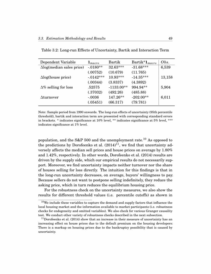
3.3. Estimation Methodology and Results 49
Table 3.2: Long-run Effects of Uncertainty, Bartik and Interaction Term
Dependent Variable 1macro Bartik Bartik*1macro Obs.∆log(median sales price) -.0180** 32.63*** -31.68*** 6,539
(.00752) (10.679) (11.765)∆log(house price) -.0142*** 10.93*** -14.35*** 13,158
(.00344) (3.8337) (4.3892)∆% selling for loss .52575 -1133.00** 994.94** 5,904
(.37032) (492.26) (485.88)∆turnover -.0036 147.26** -202.00** 6,011
(.05451) (66.317) (79.781)
Note: Sample period from 1990 onwards. The long-run effects of uncertainty (95th percentilethreshold), bartik and interaction term are presented with corresponding standard errorsin brackets. * indicates significance at 10% level, ** indicates significance at 5% level, ***indicates significance at 1% level.
population, and the S&P 500 and the unemployment rate.10 As opposed tothe predictions by Dorofeenko et al. (2014)11, we find that uncertainty ad-versely affects the median sell prices and house prices on average by 1.80%and 1.42%, respectively. In other words, Dorofeenko et al. (2014) results aredriven by the supply side, which our empirical results do not necessarily sup-port. Moreover, we find uncertainty impacts neither turnover nor the shareof houses selling for loss directly. The intuition for this findings is that inthe long-run uncertainty decreases, on average, buyers’ willingness to pay.Because sellers do not want to postpone selling indefinitely, they reduce theasking price, which in turn reduces the equilibrium housing price.
For the robustness check on the uncertainty measures, we also show theresults for different threshold values (i.e. percentile cutoffs) as shown in
10We include these variables to capture the demand and supply factors that influence thelocal housing market and the information available to market participants (i.e. robustnesschecks for endogeneity and omitted variables). We also check for various Granger causalitytest. We conduct other variety of robustness checks described in the next subsection.
11Dorofeenko et al. (2014) show that an increase in their measure of uncertainty has anincreasing effect on house prices due to the default premium on the housing developers:There is a markup on housing prices due to the bankruptcy possibility that is caused byuncertainty.

3.3. Estimation Methodology and Results 50
-.02
-.01
5-.
01-.
005
Hou
se P
rice,
Med
ian
Sol
d P
rice
80 85 90 95Threshold Value
House Price Median Sold Price
Effect of Macro Uncertainty
Figure 3.4: The Impact of Macro Uncertainty
The graph illustrates the long-run impact of Macro Uncertainty on thehouse price and the median sold price for the different threshold valueswhich are used to identify periods of high uncertainty.
Figure 3.4. Regardless of the threshold value, the sign and the significance
of the estimated→β1 for the log house price and log median sales price do not
change.12
The column three of Table 3.2 shows the long-run impact of labor demandshocks, proxied by bartik. The impact is highly significant for all dependentvariables, even after controlling for state-level unemployment. For example,one standard deviation increase in the local labor demand shock (i.e., thebartik, which is defined as change in state-level employment relative to achange in national employment), increases house prices, median sell pricesand transactions on average by .14%, .43% and 1.92%-points, respectivelyand decreases the share of houses selling for loss by 14.77%-points. Due tolinearity, the signs reverse in the case of adverse labor demand shocks - as
12All of the coefficients are significant at a 1% significance level, except for one which issignificant at the 5% level.
3.3. Estimation Methodology and Results 51
observed in most states during the Great Recession period.13
The above results indicate that the uncertainty and labor demand shocksaffect the housing market variables in opposite direction. To determine thequantitative effects of these two shocks on the housing variables, we intro-
duce an interaction term,→β3: the results are shown in the fourth column
of Table 3.2. When the labor demand shock occurs during a period of highuncertainty then, for almost every dependent variable and threshold level,the effect of uncertainty shock dominates the labor demand shock: a clear
sign change from the estimated→β2 being positive to the estimated
→β3 being
negative.
As discussed above,→β3 quantifies the homeowners’ diminished response
("wait and see effect") following a labor demand shock: 0.19% (0.013%×14.35)of the house price and 0.41% (0.013%×31.68) of the median sell price. For theexpositional purpose of the interaction term, Figure 3.5 shows the effects ofa labor demand shock with - and without uncertainty shock (using our bench-mark Macro Uncertainty shock). All dots in the graphs are significant atthe 10% significance level. The blue line (Bartik Normal Times) summarizes
the long-run impact of labor demand shocks,→β2, on the various dependent
variables, while the red line (Bartik High Uncertainty) represents the impact
of labor demand shocks in uncertainty times, i.e.→β2+
→β3. Figure 3.5 clearly
shows that when uncertain periods occur then the effect of the labor demandshock is greatly muted. These dominating uncertainty shock effects suggestthe presence of real options effects in housing market. This result is in linewith the findings of Quintin and Davis (2014), who find that uncertaintyabout housing prices kept the default rate low relative to a situation withoutuncertainty. Figure 3.6 is analogous to Figure 3.5, but with State Uncertaintyshock: the results are not overturned.
13We report the impact of a standard deviation increase due to the scale of the bartik.Mean local labor demand decreases from 1990 until 2014 by 0.004%-points, while one stan-dard deviation corresponds to 0.013%-points: For example, for the log house price, we reportan increase of 0.14% as 0.013×10.93, while the real option value is calculated similarly as
0.013 ×14.35= 0.19%, where→β3 = 14.35.
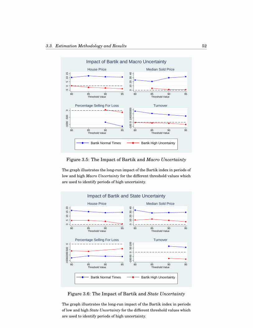
3.3. Estimation Methodology and Results 52
-50
510
15
80 85 90 95Threshold Value
House Price
010
2030
40
80 85 90 95Threshold Value
Median Sold Price-1
000
-500
0
80 85 90 95Threshold Value
Percentage Selling For Loss
-100
010
0200
300
80 85 90 95Threshold Value
Turnover
Impact of Bartik and Macro Uncertainty
Bartik Normal Times Bartik High Uncertainty
Figure 3.5: The Impact of Bartik and Macro Uncertainty
The graph illustrates the long-run impact of the Bartik index in periods oflow and high Macro Uncertainty for the different threshold values whichare used to identify periods of high uncertainty.
05
1015
20
80 85 90 95Threshold Value
House Price
010
2030
40
80 85 90 95Threshold Value
Median Sold Price
-150
0-100
0-50
00
80 85 90 95Threshold Value
Percentage Selling For Loss
-100
-50
050
100
80 85 90 95Threshold Value
Turnover
Impact of Bartik and State Uncertainty
Bartik Normal Times Bartik High Uncertainty
Figure 3.6: The Impact of Bartik and State Uncertainty
The graph illustrates the long-run impact of the Bartik index in periodsof low and high State Uncertainty for the different threshold values whichare used to identify periods of high uncertainty.
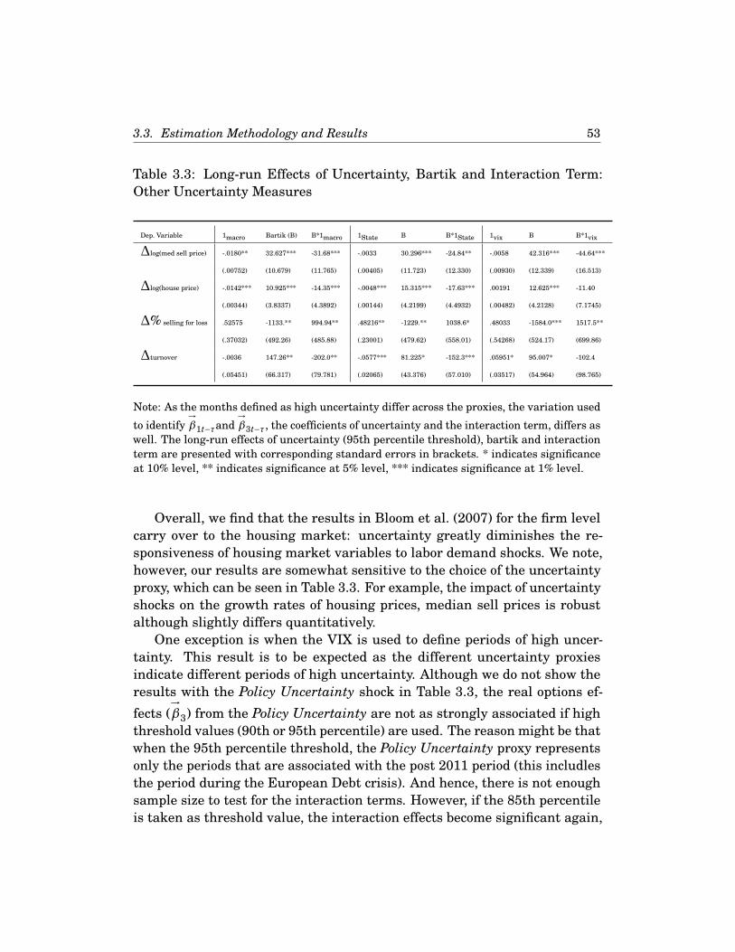
3.3. Estimation Methodology and Results 53
Table 3.3: Long-run Effects of Uncertainty, Bartik and Interaction Term:Other Uncertainty Measures
Dep. Variable 1macro Bartik (B) B*1macro 1State B B*1State 1vix B B*1vix
∆log(med sell price) -.0180** 32.627*** -31.68*** -.0033 30.296*** -24.84** -.0058 42.316*** -44.64***
(.00752) (10.679) (11.765) (.00405) (11.723) (12.330) (.00930) (12.339) (16.513)
∆log(house price) -.0142*** 10.925*** -14.35*** -.0048*** 15.315*** -17.63*** .00191 12.625*** -11.40
(.00344) (3.8337) (4.3892) (.00144) (4.2199) (4.4932) (.00482) (4.2128) (7.1745)
∆% selling for loss .52575 -1133.** 994.94** .48216** -1229.** 1038.6* .48033 -1584.0*** 1517.5**
(.37032) (492.26) (485.88) (.23001) (479.62) (558.01) (.54268) (524.17) (699.86)
∆turnover -.0036 147.26** -202.0** -.0577*** 81.225* -152.3*** .05951* 95.007* -102.4
(.05451) (66.317) (79.781) (.02065) (43.376) (57.010) (.03517) (54.964) (98.765)
Note: As the months defined as high uncertainty differ across the proxies, the variation used
to identify→β1t−τand
→β3t−τ, the coefficients of uncertainty and the interaction term, differs as
well. The long-run effects of uncertainty (95th percentile threshold), bartik and interactionterm are presented with corresponding standard errors in brackets. * indicates significanceat 10% level, ** indicates significance at 5% level, *** indicates significance at 1% level.
Overall, we find that the results in Bloom et al. (2007) for the firm levelcarry over to the housing market: uncertainty greatly diminishes the re-sponsiveness of housing market variables to labor demand shocks. We note,however, our results are somewhat sensitive to the choice of the uncertaintyproxy, which can be seen in Table 3.3. For example, the impact of uncertaintyshocks on the growth rates of housing prices, median sell prices is robustalthough slightly differs quantitatively.
One exception is when the VIX is used to define periods of high uncer-tainty. This result is to be expected as the different uncertainty proxiesindicate different periods of high uncertainty. Although we do not show theresults with the Policy Uncertainty shock in Table 3.3, the real options ef-
fects (→β3) from the Policy Uncertainty are not as strongly associated if high
threshold values (90th or 95th percentile) are used. The reason might be thatwhen the 95th percentile threshold, the Policy Uncertainty proxy representsonly the periods that are associated with the post 2011 period (this includlesthe period during the European Debt crisis). And hence, there is not enoughsample size to test for the interaction terms. However, if the 85th percentileis taken as threshold value, the interaction effects become significant again,

3.3. Estimation Methodology and Results 54
as more periods, especially the months before 2010, are classified as periodsof high uncertainty.
3.3.3 Grouping States by Housing Price VolatilityTo analyze whether the real option effect varies by regions, we sort the fiftyone U.S. states into three groups according to the unconditional housingprice volatility in each state over time, and we estimate our model (3.2) foreach one of the groups. The three groups are equal size and we refer to themas low, medium and high: Our hypothesis is to test empirically whether thechange in the responsiveness of housing market variables is larger in thestates with higher housing price volatilities compared to the lower housingprice volatilities states. Consequently, we focus on the dominant effect ofuncertainty over the labor demand shocks for each one of the groups, usingthe 95th percentile of the State Uncertainty proxy. We choose the StateUncertainty measure because we group the states according to the state-specific housing price volatility; the results are qualitatively similar, however,for the Macro Uncertainty measure. Table 3.4 shows the results for the threedifferent groups.
Table 3.4: Long-run Effects of Bartik and Interaction Term Grouped by theMagnitude of the Housing Price Volatility Over Time
Housing Price Volatility low medium highBartik (B) B*1low
state B B*1mediumstate B B*1high
state∆log(house price) 18.47** -6.85 7.055*** -9.26 21.26*** -25.0***
(7.802) (7.131) (2.596) (6.253) (6.899) (8.905)
Note: The long-run effects of bartik and interaction term based on State Uncertainty (95thpercentile threshold) are presented with corresponding standard errors in brackets groupedby housing price volatility across states. * indicates significance at 10% level, ** indicatessignificance at 5% level, *** indicates significance at 1% level.
The most striking difference between the three groups is with respect to
the significance and the magnitude of our responsiveness measure (→β3) for
the high group. As one moves away from the low to high volatility group, the
interaction term (→β3) not only increases in absolute magnitude from −6.85 to
−25 but also becomes highly statistically significant. That is, the effect of a

3.3. Estimation Methodology and Results 55
one standard deviation increase (i.e. 0.013%−points) in the interaction termchanges from −6.85×0.013= 0.09% in the low group to −25.0×0.013= 0.32%of the housing price in the high group.
3.3.4 Grouping States by the Impact of Local Labor De-mand Shocks
For the robustness check, we also sort groups by the impact of local labordemand shocks. We calculate the impact of the bartik based on our model(3.2) with housing prices as dependent variable, but estimating time-seriesregressions for each state. We include states where the bartik has a signif-icant impact (5% level) on the change in log housing prices, which resultsin 37 states. We sort these 37 states into three groups of almost equal size,depending on the magnitude of the bartik’s impact. Table 3.5 shows thelong-run effects of the bartik and the interaction term. By construction, theimpact of the bartik increases and is highly significant. The interactionterm, however, is only statistically significant for the group high, with the
sum of→β2 and
→β3 (e.g.104.9−102= 2.9) very close to zero: the net effect on
the change in log housing prices is almost zero. Moreover, an explanation forthe dominance of uncertainty over the shock for the high group, in contrastto the medium and low group, is that the larger the impact of the shock, theless responsive households are, ceteris paribus.
Table 3.5: Long-run Effects of Bartik and Interaction Term Grouped by theImpact of the Bartik in Each State
Bartik Index low medium highBartik (B) B*1low
State B B*1mediumState B B*1high
State∆log(house price) 9.835*** -5.16 52.98*** -16.1 104.9*** -102**
(2.328) (5.947) (9.703) (14.43) (21.13) (45.07)
Note: The long-run effects of bartik and interaction term based on State Uncertainty (95thpercentile threshold) are presented with corresponding standard errors in brackets groupedby housing price volatility across States. * indicates significance at 10% level, ** indicatessignificance at 5% level, *** indicates significance at 1% level.
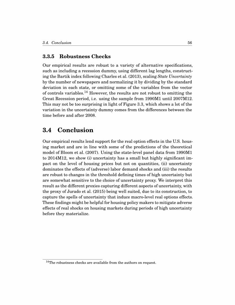
3.4. Conclusion 56
3.3.5 Robustness ChecksOur empirical results are robust to a variety of alternative specifications,such as including a recession dummy, using different lag lengths, construct-ing the Bartik index following Charles et al. (2013), scaling State Uncertaintyby the number of newspapers and normalizing it by dividing by the standarddeviation in each state, or omitting some of the variables from the vectorof controls variables.14 However, the results are not robust to omitting theGreat Recession period, i.e. using the sample from 1990M1 until 2007M12.This may not be too surprising in light of Figure 3.3, which shows a lot of thevariation in the uncertainty dummy comes from the differences between thetime before and after 2008.
3.4 ConclusionOur empirical results lend support for the real option effects in the U.S. hous-ing market and are in line with some of the predictions of the theoreticalmodel of Bloom et al. (2007). Using the state-level panel data from 1990M1to 2014M12, we show (i) uncertainty has a small but highly significant im-pact on the level of housing prices but not on quantities, (ii) uncertaintydominates the effects of (adverse) labor demand shocks and (iii) the resultsare robust to changes in the threshold defining times of high uncertainty butare somewhat sensitive to the choice of uncertainty proxy. We interpret thisresult as the different proxies capturing different aspects of uncertainty, withthe proxy of Jurado et al. (2015) being well suited, due to its construction, tocapture the spells of uncertainty that induce macro-level real options effects.These findings might be helpful for housing policy makers to mitigate adverseeffects of real shocks on housing markets during periods of high uncertaintybefore they materialize.
14The robustness checks are available from the authors on request.

3.4. Conclusion 57
Appendix
Data Appendix
Table 3.6: Uncertainty Proxies
Variable Availability Source Regional levelMacro Uncertainty 1960M1-2011M12 Jurado et al. (2015) NationalPolicy Uncertainty 1985M1-2015M2 Baker et al. (2016) NationalState Uncertainty 2000M1-2014M12 Self constructed StateVIX 1990M1-2015M2 FRED National
Table 3.7: Dependent Variables
Variable Availability Source Regional levelHouse Price 1975M1-2014M12 Freddie&Mac StateMedian Sales Price 1996M4-2014M12 Zillow Database State% Selling For Loss 1998M1-2014M12 Zillow Database StateTotal Turnover 1998M1-2014M12 Zillow Database State
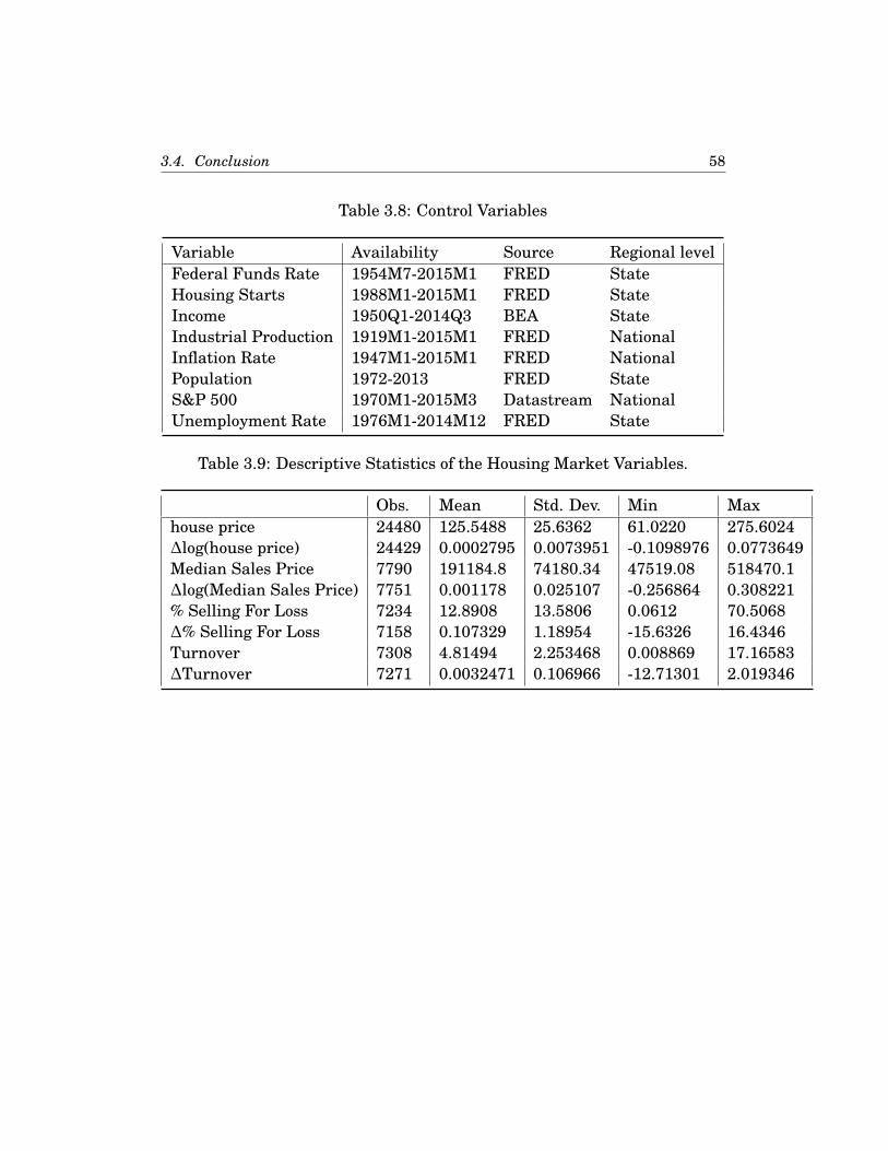
3.4. Conclusion 58
Table 3.8: Control Variables
Variable Availability Source Regional levelFederal Funds Rate 1954M7-2015M1 FRED StateHousing Starts 1988M1-2015M1 FRED StateIncome 1950Q1-2014Q3 BEA StateIndustrial Production 1919M1-2015M1 FRED NationalInflation Rate 1947M1-2015M1 FRED NationalPopulation 1972-2013 FRED StateS&P 500 1970M1-2015M3 Datastream NationalUnemployment Rate 1976M1-2014M12 FRED State
Table 3.9: Descriptive Statistics of the Housing Market Variables.
Obs. Mean Std. Dev. Min Maxhouse price 24480 125.5488 25.6362 61.0220 275.6024∆log(house price) 24429 0.0002795 0.0073951 -0.1098976 0.0773649Median Sales Price 7790 191184.8 74180.34 47519.08 518470.1∆log(Median Sales Price) 7751 0.001178 0.025107 -0.256864 0.308221% Selling For Loss 7234 12.8908 13.5806 0.0612 70.5068∆% Selling For Loss 7158 0.107329 1.18954 -15.6326 16.4346Turnover 7308 4.81494 2.253468 0.008869 17.16583∆Turnover 7271 0.0032471 0.106966 -12.71301 2.019346

3.4. Conclusion 59
Table 3.10: Descriptive Statistics of the Uncertainty Measures and thebartik.
Obs. Mean Std. Dev. Min MaxMacro Uncertainty 264*51 0.67773 0.0961123 0.568981 1.130619Policy Uncertainty 300*51 106.3401 34.38186 57.20262 245.1267State Uncertainty 9180 18.23878 7.730284 0 233VIX 300*51 19.9604 7.730284 10.82 62.64bartik 15249 -0.000041 0.0001304 -0.002793 0.0009686
Sorted States in Subsection 3.3.3
Table 3.11: Sorted States, According to their Unconditional Housing PriceVolatility over Time.
low medium highAlabama Alaska ArizonaArkansas Colorado CaliforniaGeorgia Delaware Connecticut
Iowa Idaho District of ColumbiaIndiana Illinois FloridaKansas Louisiana Hawaii
Kentucky Maine MassachusettsMissouri Michigan Maryland
Mississippi Minnesota New HampshireNorth Carolina Montana New Jersey
Nebraska North Dakota NevadaNew Mexico Oklahoma New York
Ohio Pennsylvania OregonSouth Carolina Texas Rhode IslandSouth Dakota Utah Virginia
Tennessee Vermont WashingtonWisconsin West Virginia Wyoming

3.4. Conclusion 60
Sorted States in Subsection 3.3.4
Table 3.12: Sorted States, According to the Impact of the bartik in EachState.
low medium highColorado Arkansas AlaskaGeorgia Kansas Arizona
Iowa Massachusetts District of ColumbiaIllinois Maryland Delaware
Kentucky Minnesota HawaiiLouisiana Missouri MaineMichigan North Dakota New Hampshire
Mississippi Nebraska New MexicoNorth Dakota New Jersey Oregon
New York South Carolina South DakotaOklahoma Virginia West VirginiaTennessee Washington Wyoming
Texas

CHAPTER 4
Uncertainty and Trade
This chapter consists of two sections. Section 4.1 quantifies the impact ofmacroeconomic uncertainty shocks on disaggregated German import flowsusing a classification scheme1 from the German Engineering Association(www.vdma.org), which categorizes manufacturing goods into intermediateand final goods. In order to enhance the understanding of this classificationscheme, section 4.22 applies this scheme to European trade data and providesdescriptive statistics as well as causality analyses of trade flows of the EU-27countries.
4.1 Uncertainty and Trade: Evidence from Ger-many
Abstract: This paper quantifies the impact of macroeconomic uncertaintyshocks on the disaggregated German import flows. Structural VAR (SVAR)estimations reveal that a one standard deviation increase in macroeconomicuncertainty induces a decline in total import, import of intermediate man-ufacturing goods and import of final manufacturing goods by 1.04%, 1.43%and 1.44%, respectively. The findings suggest that uncertainty shocks in one
1I am grateful to Prof. Dr. Richard Frensch and the Institute for East and EasternEuropean Studies in Regensburg (IOS) for sharing their data with me.
2This section is based on joint work with Stephan Huber and was published in a journal(Huber and Thanh, 2017).
61

4.1. Uncertainty and Trade: Evidence from Germany 62
country affect production in another through the trade channel.
4.1.1 IntroductionUncertainty shocks are considered to be an important driver of the real econ-omy. Christiano et al. (2014) argue that time-varying uncertainty is the mostimportant driver of the business cycle and other studies suggest a decline ininvestment in response to uncertainty shocks (e.g., Bernanke, 1983; Bloom,2009; Meinen and Roehe, 2017). In the same vein, Karnizova and Li (2014)find that the economic policy uncertainty measure proposed by Baker et al.(2016) is a robust predictor of U.S. recessions. Moreover, Leduc and Liu (2016)show that an increase in uncertainty induces a rise in the unemploymentrate and Dorofeenko et al. (2014) conclude that uncertainty shocks accountfor over 90% of the U.S. house price volatility.
While most studies focus on the impact of uncertainty within a coun-try, there are also works on the cross-border effects of uncertainty shocks.Colombo (2013) estimates Structural Vector Autogregression (SVAR) modelsand documents that a one standard deviation U.S. economic policy uncer-tainty shock decreases European industrial production by 0.12%. Similarly,the SVAR estimations of Mumtaz and Theodoridis (2015) show that a onestandard deviation increase in the volatility of U.S. real activity shocks leadsto a 1% decline in U.K. GDP.
Nevertheless, it remains unclear through which channel(s) a domesticuncertainty shock affects real activity in foreign economies. The current pa-per seeks to clarify this question and investigates whether the trade channelplays an important role in transmitting uncertainty shocks in one countryon production in another. The theoretical model of Novy and Taylor (2014)predicts that manufacturing firms cut the import of intermediate goods inresponse to a rise in uncertainty, while Bloom (2014) suggests the rise ofprecautionary savings and thus lesser consumption which, in turn, trans-lates into a decrease of the import of final consumption goods during periodsof high uncertainty. Using German disaggregated trade data, I empiricallytest these two predictions. SVAR estimations indicate that a one standarddeviation increase in uncertainty lowers the import of intermediate manufac-turing goods, the import of final manufacturing goods and the total volumeof import in the middle-run by 1.43%, 1.44% and 1.04%, respectively.
Subsection 4.1.2 presents the data and the estimation specification, whilesubsection 4.1.3 presents the estimation results. Finally, subsection 4.1.4

4.1. Uncertainty and Trade: Evidence from Germany 63
concludes.
4.1.2 Data and Econometric SpecificationI use disaggregated Combined Nomenclature 8 digit-level monthly Comexttrade data from Eurostat from 1996M6 to 2015M33 and a classificationscheme from the German Engineering Association (www.vdma.org) that cat-egorizes traded manufacturing goods into parts, components and final goods.In this section, I interpret both parts and components as intermediate goods.On average, 11% of total import is classified as the import of manufactur-ing goods. Table 4.3 in the Appendix of section 4.2 shows examples of themost traded intermediate and final goods and section 4.2 provides a detaileddiscussion on this classification scheme and the disaggregated trade data.
Furthermore, I use a measure for the German macroeconomic uncertainty(German Macro Uncertainty) which is analogous the Macro Uncertainty pro-posed by Jurado et al. (2015), but proxies the average uncertainty of Germanmacroeconomic series. German Macro Uncertainty is provided by Meinenand Roehe (2017) who use 143 macroeconomic time series for the computa-tion. This measure captures the predictability of the overall macroeconomicenvironment; the less predictable the macroeconomic variables, the higherthe macroeconomic uncertainty. I use the one-month-ahead measure, sincethe data are at a monthly frequency. Using a similar measure for macroeco-nomic uncertainty which is proposed by Rossi and Sekhposyan (2015) leadsto the same conclusions4.
I also include the DAX, the German industrial production in the manu-facturing section (production) and the German employment (employment)in the SVAR estimation. These data were collected from Thomson ReutersDatastream. The import data, production and employment are seasonallyadjusted, and all variables are Hodrick-Prescott (HP) detrended (λ=129,600),analogous to Bloom (2009) and Novy and Taylor (2014).
I use the following SVAR representation:
B0 yt = B(L)yt−p + e t, (4.1)
3The Macro Uncertainty measure is not available for earlier periods.4The estimation results are presented in the Appendix.
4.1. Uncertainty and Trade: Evidence from Germany 64
where yt =
log(DAX )
German Macro Uncertaintylog(production)
log(employment)log(importvariable)
t
, e t is the vector of structural inno-
vations, B(L) an autoregressive lag-polynomia and B0 the matrix containingthe contemporaneous relationships between the reduced-form residuals andthe structural innovations. I use a standard Cholesky decomposition impos-ing a lower triangular matrix to identify B0. Following Bloom (2009) andNovy and Taylor (2014), I use the ordering5 log(DAX ), German Macro Un-certainty, log(production), log(employment) and log(importvariable). Ifollow the recommendation of the Schwarz Criterion and decided to choosetwo lags in the benchmark specification. However, the results are robust toalternative lag specifications.
4.1.3 Estimation ResultsFigure 4.1 depicts the impulse response functions of the import variables to aone standard deviation shock to German Macro Uncertainty. A one standarddeviation increase in German Macro Uncertainty significantly lowers theimport of intermediate manufacturing goods and final manufacturing goodsas well as the total volume of import in the middle-run, reaching a maximumlevel of impact of 1.43%, 1.44% and 1.04%, respectively. The reduction of theimport of intermediate goods in response to an increase in uncertainty is inline with the prediction of the model of Novy and Taylor (2014). In the model,firms face fixed costs of ordering from abroad and thus store intermediategoods according to an inventory policy. Firms respond to uncertainty shocksby contracting their inventory policy and cutting their import of intermediategoods. On the other hand, the decline of the import of final goods indicates therise of precautionary savings and therefore lower consumption as suggestedby Bloom (2014). It is worth nothing that the reactions of the import ofintermediate goods and the import of final goods to an uncertainty shock arequalitatively and quantitatively similar. This observation indicates that thecutting of foreign import of intermediate goods is similar to the reduction ofconsumption of goods from abroad. Moreover, while Bloom (2009) finds thatfollowing an uncertainty shock output, employment and productivity decline
5The main results are robust to alternative order specifications.

4.1. Uncertainty and Trade: Evidence from Germany 65
-.02
-.01
0
.01
0 5 10 15 20
Import of Intermediate Goods
-.02
-.01
0
.01
0 5 10 15 20
Import of Final Goods
-.02
-.01
0
.01
0 5 10 15 20
Import of Total Manufacturing Goods
-.02
-.01
0
.01
0 5 10 15 20
Total Volume of Import
German Macro Uncertainty
Figure 4.1: Impulse Response Function of Import Variablesto a German Macro Uncertainty Shock
Note: The sample period is 1996M6-2015M7. The figure displays theresponse of import variables to a one standard deviation German MacroUncertainty shock. The shaded areas denote the 95% confidence inter-vals from multivariate parametric bootstrap procedures with 2000 repli-cations.
for some periods and overshoot in the recovery phase, the import variablesdo not show a comparable overshooting reaction.
Figure 4.2 illustrates the relative importance of a German Macro Un-certainty innovation in explaining the forecast error variance of the importvariables. The forecast error variance decomposition confirms the findingthat the impact of a German Macro Uncertainty shock is more important inthe middle-run and not in the short-run. There is a very low level of contri-bution of an innovation in German Macro Uncertainty to the total forecasterror variances of the import variables in the first 5 months, but the levelsof contribution rise sharply in the middle-run and reach 35% (intermediategoods), 25% (final goods) and 33% (total volume of import) after 15 months.

4.1. Uncertainty and Trade: Evidence from Germany 66
0
.2
.4
.6
0 5 10 15 20
Import of Intermediate Goods
0
.2
.4
.6
0 5 10 15 20
Import of Final Goods
0
.2
.4
.6
0 5 10 15 20
Impoft of Total Manufacturing Goods
0
.2
.4
.6
0 5 10 15 20
Total Volume of Import
German Macro Uncertainty
Figure 4.2: Forecast Error Variance Decomposition Due to anInnovation in German Macro Uncertainty
Note: The sample period is 1996M6-2015M3. The shaded areas denotethe 95% confidence intervals from multivariate parametric bootstrap pro-cedures with 2000 replications.
4.1.4 ConclusionI use German data to investigate the impact of macroeconomic uncertaintyon import flows. SVAR estimations reveal that a rise in Macro Uncertaintylowers the import of intermediate manufacturing goods, final manufacturinggoods and the total volume of import. The magnitude of reaction to an uncer-tainty shock of the import of intermediate goods is comparable to the one ofthe import of final goods. The reduction of import following an uncertaintyshock in a country equates with a lower export of its trade partners whichcools down the production in those partner countries. This mechanism helpsto understand why there are cross-border spillover effects of uncertaintyshocks.

4.1. Uncertainty and Trade: Evidence from Germany 67
Appendix
Data Appendix
• Disaggregated trade data are collected from Eurostat(http://ec.europa.eu/eurostat/de/data/database).
• German Macro Uncertainty is provided by Meinen and Roehe (2017)(http://www.sciencedirect.com/science/article/pii/S0014292116302239).
• Macroeconomic uncertainty by Rossi and Sekhposyan (2015): the au-thors propose an alternative measure of macroeconomic uncertaintywhich quantifies the unpredictable components of GDP. They extractthe unforecastable component from GDP and, subsequently, evaluatethe cumulative density of forecast errors at the actual realized forecasterror. Meinen and Roehe (2017) follow the approach of Rossi and Sekh-posyan (2015) and calculate for a wide range of macroeconomic vari-ables a corresponding uncertainty measure and compute the arithmeticmean across all uncertainty series. This arithmetic mean measure ofuncertainty, which is based on a multitude of macroeconomic variables,is used for the computation of 4.3. This measure for Germany is pro-vided by Meinen and Roehe (2017)(http://www.sciencedirect.com/science/article/pii/S0014292116302239).

4.1. Uncertainty and Trade: Evidence from Germany 68
Supplementary Graph
-.01
-.005
0
.005
.01
0 5 10 15 20
Import of Intermediate Goods
-.02
-.01
0
.01
0 5 10 15 20
Import of Final Goods
-.01
0
.01
0 5 10 15 20
Import of Total Manufacturing Goods
-.01
-.005
0
.005
0 5 10 15 20
Total Volume of Import
Macroeconomic Uncertainty (Rossi & Sekhposyan)
Figure 4.3: Response of Import Variables to a One StandardDeviation Macroeconomic Uncertainty Shock Which Is Pro-posed by Rossi and Sekhposyan (2015)
Note: The sample period is 1996M7-2015M3. The macroeconomic uncer-tainty measure by Rossi and Sekhposyan (2015) for Germany is computedand provided by Meinen and Roehe (2017).

4.2. Vertical Specialization in the EU and the Causality of Trade. 69
4.2 Vertical Specialization in the EU and theCausality of Trade.
Abstract: We6 use a novel classification scheme to identify three stages ofproduction in the manufacturing sector: parts, components, and final goods.In particular, we offer evidence on the revealed comparative advantage ofthe EU-27 countries concerning the three vertically separated stages of pro-duction. Moreover, we investigate whether, and if so how, imports of parts,and components can work as a predictor for the exports of final goods. Wefind that countries specialize at different stages of production, and that com-ponents are Granger causal for the export of final goods in many countrieswith a lag of three months.
Acknowledgement to prior publication in Appplied Economics Letters:This section is joint work with Stephan Huber and was published in Ap-plied Economics Letters, 2017, 24 (5), 329-333, copyright Taylor & Francis,available online: http://dx.doi.org/10.1080/13504851.2016.1186791
6We are grateful to the Institute for East and Eastern European Studies in Regensburg(IOS) for sharing their data with us. In particular, we are grateful to Richard Frensch,Volkhart Vincentz as well as all IOS-seminar participants.

4.2. Vertical Specialization in the EU and the Causality of Trade. 70
4.2.1 IntroductionThe share of intermediates in intra-EU trade is increasing and reaches al-most 50% nowadays.7 Although some widely received articles, such as Hum-mels et al. (2001), Feenstra (1998), or Grossman and Rossi-Hansberg (2006),have addressed the issue of how countries specialize along the vertical produc-tion chain, surprisingly little is known about the comparative advantage andthe causal interrelationship of international trade in parts, components, andfinal goods. The research gap can be explained with a lack of data that allowsto distinguish traded goods at vertically separated stages of production thatgoes beyond the dichotomy of ‘parts&components’ and ‘final goods’. We aim tofill this gap by using a novel categorization scheme compiled by experts of theGerman Engineering Association (www.vdma.org), which categorizes tradedmanufacturing goods at the highly disaggregated CN-8 digit-level into threevertically separated stages of production: (1) parts, (2) components, and (3)final goods. Overall, we identify 245 products as parts, 329 products as com-ponents, and 1058 products as final goods within the manufacturing sector.8
This trisection allows us to overview the comparative advantage of countriesat different stages of production and to investigate whether the imports ofparts and components can help to predict exports of goods at the final stageof assembling.
In our analysis, we employ Granger causality tests revealing that importsof parts and components help to predict the export of final goods. This holdsespecially true for countries with a high revealed comparative advantagein the export of final goods. However, the import of components are oftensufficient to improve the prediction about exports of final goods. The chosenlag length is quite often three month, which can be interpret as the time ittakes to assemble and export a final good. The causal impact of less differen-tiated imports in parts, however, seems to play a minor role. The intuition ofthis result is that components have a smaller range of use in the productionsystem and hence are often specifically build to work as a preliminary input
7We refer to Guerrieri and Caffarelli (2012) for an overview how the international frag-mentation of production has developed.
8Parts contains commodities like electronic instruments, mechanical seals, sewing ma-chine needles with single flat shank, and spinning rings. The intermediate class componentscontains commodities such as engines and motors, air conditioning machines, temperatureregulators, or articulated shafts. Final goods classify manufacturing commodities such asgas turbines, digger, lifts, or mobile cranes. For some further examples of the categorisationwe refer to Table 4.3 in the Appendix.

4.2. Vertical Specialization in the EU and the Causality of Trade. 71
for a small range of final manufacturing goods.The remainder of the paper is structured as follows. Subsection 4.2.2 in-
troduces the data and offers some descriptive facts concerning the countries’revealed comparative advantage. Subsection 4.2.3 asks, whether imports ofparts and components are Granger causal for exporting final goods. Subsec-tion 4.2.4 concludes.
4.2.2 Data and Comparative AdvantageWe use de-seasonalized (X-12-ARIMA adjusted) monthly COMEXT tradedata from Eurostat from 1988M1 to 2015M8 for 27 EU countries. Table 4.1contains the number of observations for each country, which vary from 188to 332, as well as the share of exports and imports captured by parts (p),components (c), and final goods ( f ), which vary from about three percent(Ireland and Greece) to over twenty percent (Italy and Germany9).
Table 4.1 contains the Revealed Comparative Advantage index (RCA)10
for parts, components, and other goods (o) for exports and imports, respec-tively. We calculate the RCA using the average export and import flows from2004 to 2013. In this time span our sample is balanced and it is long enoughto smooth out disturbing effects from temporarily economic shocks. The re-sults reveal that some countries, like Austria, Germany, Denmark, Finland,Italy, and Sweden do have a general comparative advantage in exports ofmanufacturing goods, while other countries, like Czech Republic, Portugal,Romania, Slovakia, and Slovenia specialize only in earlier stages of produc-tion.
An interesting observation is Germany, since recent literature, such asSinn (2006), emphasize that Germany is a ‘bazaar economy’ which importsearly stages of production to assemble them and export final goods. Our re-sults support this hypothesis: Germany has a RCA in importing parts (1.21)and components (1.18) and a relative high RCA in exporting final goods (1.52)compared to the RCA in exporting parts (1.23) and components (1.4). TheRCA of Portugal, Romania, and Slovakia in the export of components is alsoremarkably high. This could be driven by some large firms of the automotiveindustry who offshore early and intermediate stages of production into these
9Germany is denoted as “DEU".10It is defined by RCA i j = xi j /
∑j xi j∑
i xi j /∑
j∑
i xi j, where xi j denotes the exports or imports in good
class i of the declaring country j.

4.2. Vertical Specialization in the EU and the Causality of Trade. 72
countries.
Table 4.1: Revealed Comparative Advantage in Parts, Components and FinalGoods
RCAexp RCAex
c RCAexf RCAex
o RCAimp RCAim
c RCAimf RCAim
o SEx SIm Obs.
AUT 1.22 1.22 1.35 .95 1.41 1.54 1.48 .95 .21 .157 248BEL .64 .65 .46 1.07 .77 .83 .76 1.02 .078 .079 200BGR .58 .79 .52 1.07 .85 .72 1.35 .99 .086 .115 188CYP .16 .08 .46 1.11 .46 .41 .92 1.03 .048 .077 188CZE 1.37 1 .98 .99 1.38 1.35 1.25 .97 .168 .14 188DEU 1.23 1.4 1.52 .93 1.21 1.18 1.05 .99 .231 .108 332DNK 1.39 1.17 1.28 .96 1.3 1.37 1.16 .98 .194 .124 332ESP .55 .54 .63 1.06 .77 .89 .91 1.01 .085 .095 332EST .73 .24 .75 1.05 .63 .72 1.3 1 .096 .107 188FIN 1.22 1.03 1.48 .95 1.12 1.23 1.15 .98 .193 .121 248FRA .77 .88 .7 1.04 .96 .96 1.01 1 .106 .099 332GBR .92 .79 .79 1.03 .87 .83 .93 1.01 .128 .093 332GRC .22 .12 .33 1.11 .5 .48 .77 1.04 .035 .077 332HUN .95 .82 .76 1.03 1.32 1.53 1.8 .94 .12 .18 188IRL .41 .14 .24 1.11 .79 .47 .73 1.03 .034 .072 332ITA 1.51 1.69 1.59 .91 .86 1.08 .86 1.01 .256 .09 332LTU .32 .43 .65 1.07 .63 .61 1.1 1.01 .079 .09 188LUX .86 .81 .31 1.07 .81 .57 .59 1.04 .078 .066 200LVA .33 .38 .65 1.07 .65 .7 1.31 1 .076 .109 188MLT .4 .18 .36 1.1 .65 .33 .78 1.03 .043 .07 188NLD .92 .45 .61 1.05 1.03 .67 .7 1.02 .088 .077 332POL .63 .66 .84 1.04 .94 1.2 1.45 .97 .115 .134 188PRT .33 1.01 .57 1.06 .7 .64 .95 1.02 .073 .091 332ROM .84 1.21 .52 1.05 1.18 1.05 1.46 .97 .104 .139 188SVK .82 1.07 .55 1.05 1.05 1.11 1.08 .99 .104 .113 188SVN 1.2 .88 .93 1 .92 1.02 1.1 1 .152 .109 188SWE 1.33 1.31 1.01 .98 1.28 1.32 1.22 .97 .178 .135 248
SEx and SIm denote the share of total export and the share of total import which is catego-rized as manufacturing goods, respectively.
4.2.3 CausalityIn this section, we ask whether imports of preliminary and intermediategoods are Granger causal for the exports of final goods. To investigate whether

4.2. Vertical Specialization in the EU and the Causality of Trade. 73
the import of parts (imp) and components (imc) is Granger causal for theexport of final goods (ex f ), we estimate for each country:
∆log(ex f )t =β0 +p∑
j=1∆log(imp)t− jβ j
+p∑
j=1∆log(imc)t− jγ j
+p∑
j=1∆log(ex f )t− jδ j +ut. (4.2)
whereby we use the Akaike (AIC) and Schwarz information criterion (SIC) tochoose an appropriate lag length p. In order to test the relevance of imp andimc, respectively, we employ two tests: The first one is a Granger causalitytest with:
H0 :β1 = ·· · =βp = γ1 = ·· · = γp = 0. (4.3)
The second test checks whether an increase of imports in parts and compo-nents lead to an increase of exports of final goods:
H0 :β1 +·· ·+βp +γ1 +·· ·+γp ≤ 0. (4.4)
If both tests can be rejected, imp and imc are positive Granger causal forex f .
Instead of presenting 27 regressions and its corresponding test statistics,we summarize our results in Table 4.2. The fourth column denotes the resultsfor estimating and testing equation (4.2). To test whether the imports of partsor components solely determine the exports of final goods, we show in thesecond and third column the results for specifications which omit from ourbaseline specification components (im2) and parts (im1), respectively. Weabbreviate the results as follows: a star (∗) indicates a rejection of the firsttest, a plus (+) denotes a rejection of the second test, both at a 5% significancelevel. The superscript number denotes the chosen lag length following theSchwarz Information Criterion (SIC) and the Akaike information criterion(AIC). The table contains results for both selection criteria, whereby theresults for the AIC are shown in brackets.
Following the SIC, imports of parts are positive Granger causal for Italy
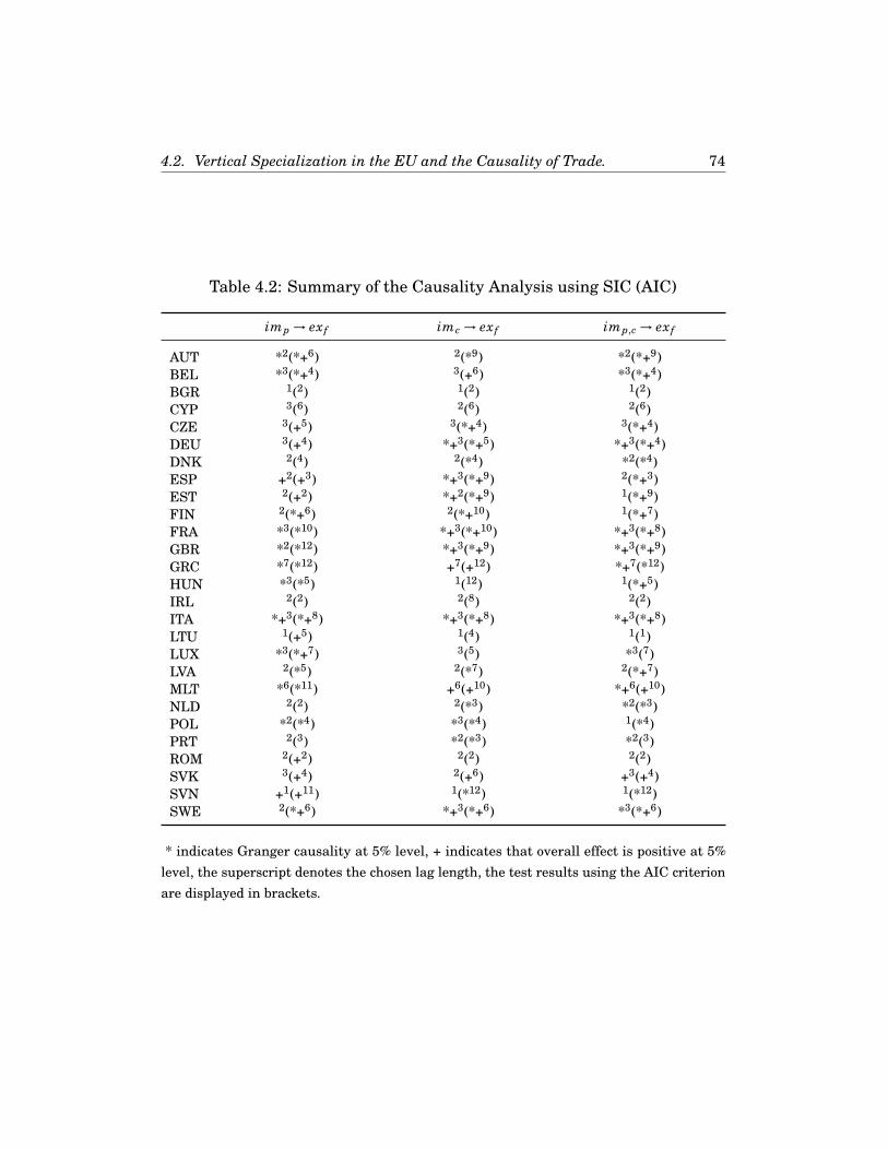
4.2. Vertical Specialization in the EU and the Causality of Trade. 74
Table 4.2: Summary of the Causality Analysis using SIC (AIC)
imp → ex f imc → ex f imp,c → ex f
AUT *2(*+6) 2(*9) *2(*+9)BEL *3(*+4) 3(+6) *3(*+4)BGR 1(2) 1(2) 1(2)CYP 3(6) 2(6) 2(6)CZE 3(+5) 3(*+4) 3(*+4)DEU 3(+4) *+3(*+5) *+3(*+4)DNK 2(4) 2(*4) *2(*4)ESP +2(+3) *+3(*+9) 2(*+3)EST 2(+2) *+2(*+9) 1(*+9)FIN 2(*+6) 2(*+10) 1(*+7)FRA *3(*10) *+3(*+10) *+3(*+8)GBR *2(*12) *+3(*+9) *+3(*+9)GRC *7(*12) +7(+12) *+7(*12)HUN *3(*5) 1(12) 1(*+5)IRL 2(2) 2(8) 2(2)ITA *+3(*+8) *+3(*+8) *+3(*+8)LTU 1(+5) 1(4) 1(1)LUX *3(*+7) 3(5) *3(7)LVA 2(*5) 2(*7) 2(*+7)MLT *6(*11) +6(+10) *+6(+10)NLD 2(2) 2(*3) *2(*3)POL *2(*4) *3(*4) 1(*4)PRT 2(3) *2(*3) *2(3)ROM 2(+2) 2(2) 2(2)SVK 3(+4) 2(+6) +3(+4)SVN +1(+11) 1(*12) 1(*12)SWE 2(*+6) *+3(*+6) *3(*+6)
* indicates Granger causality at 5% level, + indicates that overall effect is positive at 5%level, the superscript denotes the chosen lag length, the test results using the AIC criterionare displayed in brackets.

4.2. Vertical Specialization in the EU and the Causality of Trade. 75
and imports of components are positive Granger causal for Germany, Spain,Estonia, France, Great Britain, Italy, and Sweden. With the exception ofFrance and Great Britain, the results reveal that it is more likely to yieldsignificant results for countries that have a comparative advantage in theexport of final goods. For Estonia, the superior lag length is two, for all othercountries it is three. This can be interpret as the time it takes for componentsto be assembled to final goods and in turn be exported. As the last columnshows, the common inclusion of imports of parts and components yields sig-nificant and positive Granger causalities for Germany, France, Great Britain,Greece, Italy, and Malta. However, these Granger causalities are mostlydriven by the imports of components, as the previous results can tell.
To explain the fact that we fail to find (positive) Granger causalities forall countries, one has to consider the nature and the limitations of our data:First, for some countries, the time series is rather short. This makes it diffi-cult to find robust results, especially because we apply robust Newey-West11
standard errors in our autoregressive model. More sophisticated modelswould require further information, such as which manufacturing parts areused to produce certain components and final goods. Second, imports ofparts and components are not the only input-source to produce final goods.However, our data does not allow to capture non-manufacturing inputs fromabroad or inputs that are not imported. Thus, it is unlikely to find causal-ity for countries that export only a small share of their exports within themanufacturing goods that we capture with part, components, and final goods.This share is shown for the imports and the exports in Table 4.1. Third, wecannot control for the imports of parts and components that are used for selfconsumption and not to produce final goods for the export sector.
4.2.4 Concluding RemarksThis letter provides novel evidence on the export and import specializationconcerning three different stages of production for EU-27 countries. More-over, this paper shows that a more detailed classification of traded goods yieldsignificant improvements of the prediction of exports of final goods, becauseit is predominantly the import of components that drives the exports of finalgoods. Parts, however, seem to play a minor role. Thus, countries with arevealed comparative advantage in the export of final goods tend to import
11See Newey and West (1987).

4.2. Vertical Specialization in the EU and the Causality of Trade. 76
parts and components in order to assemble and export final goods. Of course,the results are borne by a simple empirical model and the time series arerather short for some countries. Nevertheless, we think our exercise helps tounderstand the global production sharing process further. Overall, we hopethat this letter encourages future empiricism to apply more elaborated anddetailed classification schemes.
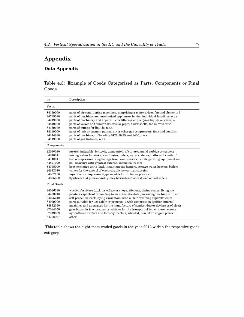
4.2. Vertical Specialization in the EU and the Causality of Trade. 77
Appendix
Data Appendix
Table 4.3: Example of Goods Categorized as Parts, Components or FinalGoods
nc Description
Parts:
84159000 parts of air conditioning machines, comprising a motor-driven fan and elements f84799080 parts of machines and mechanical appliances having individual functions, n.e.s.84219900 parts of machinery and apparatus for filtering or purifying liquids or gases, n.84819000 parts of valves and similar articles for pipes, boiler shells, tanks, vats or th84139100 parts of pumps for liquids, n.e.s.84149000 parts of : air or vacuum pumps, air or other gas compressors, fans and ventilati84314980 parts of machinery of heading 8426, 8429 and 8430, n.e.s.84119900 parts of gas turbines, n.e.s.
Components:
82090020 inserts, indexable, for tools, unmounted, of sintered metal carbide or cermets84818011 mixing valves for sinks, washbasins, bidets, water cisterns, baths and similar f84148011 turbocompressors, single-stage (excl. compressors for refrigerating equipment an84821090 ball bearings with greatest external diameter, 30 mm84195000 heat-exchange units (excl. instantaneous heaters, storage water heaters, boilers84812010 valves for the control of oleohydraulic power transmission84807100 injection or compression-type moulds for rubber or plastics84835080 flywheels and pulleys, incl. pulley blocks (excl. of cast iron or cast steel)
Final Goods:
94036090 wooden furniture (excl. for offices or shops, kitchens, dining rooms, living roo84433210 printers capable of connecting to an automatic data processing machine or to a n84295210 self-propelled track-laying excavators, with a 360 °revolving superstructure84099900 parts suitable for use solely or principally with compression-ignition internal84862090 machines and apparatus for the manufacture of semiconductor devices or of electr87084050 gear boxes for tractors, motor vehicles for the transport of ten or more persons87019039 agricultural tractors and forestry tractors, wheeled, new, of an engine power84798997 other
This table shows the eight most traded goods in the year 2012 within the respective goodscategory.
CHAPTER 5
Conclusion
The goal of this dissertation is to expand the understanding of the impactof economic uncertainty on economic activities by analyzing empirical data.There are robust and significant negative effects of uncertainty on financial,housing and trade markets, which indicate the occurrence of real optionseffects in those markets during periods of high uncertainty.
In chapter 2, time series estimations reveal that economic uncertaintyshocks substantially impede the number of U.S. initial public offerings. Boththe reduction of newly filed IPOs and the increase of withdrawn IPOs con-tribute to the overall decrease of the number of IPOs. Moreover, high eco-nomic uncertainty also depresses the IPO market condition variables, such asoutput, stock market growth and investor sentiment. Since high uncertaintyshocks often persist for multiple quarters, they can hamper IPO issues fora considerable amount of periods and, thus, create cold IPO market phases.As high uncertainty dissolves, IPO-interested firms may want to go publicin the same periods which could, in turn, generate hot IPO market phases.The described connection between uncertainty and the IPO timing providesan alternative and complementary explanation for the existence of IPO issuecycles.
Chapter 3 illuminates the impact of economic uncertainty on the housingmarket using a U.S. state level panel data set. We find a significant negativeimpact of uncertainty on the housing prices. Moreover, during periods ofhigh uncertainty, housing market variables, such as housing price, mediansell price, turnover rate and percentage of houses sold for loss are less re-
78

79
sponsive to labor demand shocks than in periods of low uncertainty. Thisfinding suggests that the effect of uncertainty shocks dominates that of labordemand shocks and indicates that housing market variables react differentlyin periods of high uncertainty, which should be taken into account by policymakers.
Finally, chapter 4 quantifies the impact of macroeconomic uncertaintyon German disaggregated import flows with SVAR estimations. The resultsindicate that an increase in uncertainty reduces the import of intermediateand final manufacturing goods as well as the total volume of import. Thereduction of imports following an uncertainty shock offers a possible expla-nation for the question of why an uncertainty shock in one country affectseconomic activity in another.
For future research, further analyses on the lower responsiveness of eco-nomic agents to changes in the economic environment during periods of higheconomic uncertainty might be fruitful. In light of the findings of this disser-tation, I conjecture that, for example, the impact of fiscal stimulus packagesor monetary policy is less effective during times of high uncertainty. Fur-thermore, it might be rewarding to study the nonlinear effects of uncertaintyshocks, since the effects of an increase in uncertainty may not be symmet-rical with the effects of a decline in uncertainty. Other fertile ground forcontinuing research might be the identification of potential methods whichcould help to reduce the level of uncertainty. For instance, creditable policycommitment may remove the layer of uncertainty and encourage economicactivity.

References
Aastveit, Knut Are, Gisle James Natvik, and Sergio Sola, “Economic Uncertainty andthe Effectiveness of Monetary Policy,” Technical Report, Norges Bank 2013. [Cited on page 42.]
Alti, Aydogan, “IPO Market Timing,” The Review of Financial Studies, 2005, 18 (3), 1105–1138. [Cited on pages 12 and 22.]
Arellano, Cristina, Yan Bai, and Patrick J. Kehoe, “Financial frictions and fluctuationsin volatility,” Staff Report 466, Federal Reserve Bank of Minneapolis 2012. [Cited on page 2.]
Bachmann, Rüdiger and Christian Bayer, “"Wait-and-See" business cycles?,” Journalof Monetary Economics, 2013, 60 (6), 704 – 719. [Cited on page 15.]
Baker, Scott R, Nicholas Bloom, and Steven J Davis, “Measuring Economic PolicyUncertainty,” The Quarterly Journal of Economics, 2016. [Cited on pages 4, 11, 17, 32, 39, 43, 45, 57, and 62.]
Bansal, Ravi, Dana Kiku, Ivan Shaliastovich, and Amir Yaron, “Volatility, the Macroe-conomy, and Asset Prices,” The Journal of Finance, December 2014, 69 (6), 2471–2511.[Cited on page 15.]
Bartik, Timothy J., Who Benefits from State and Local Economic Development Policies?number wbsle. In ‘Books from Upjohn Press.’, W.E. Upjohn Institute for EmploymentResearch, 1991. [Cited on page 42.]
Benveniste, Lawrence M., Alexander Ljungqvist, William J. Wilhelm, and XiaoyunYu, “Evidence of Information Spillovers in the Production of Investment Banking Ser-vices,” The Journal of Finance, 2003, 58 (2), 577–608. [Cited on page 12.]
Bernanke, Ben S., “Irreversibility, Uncertainty, and Cyclical Investment,” The QuarterlyJournal of Economics, 1983, 98 (1), 85–106. [Cited on pages 2, 13, 15, and 62.]
Bhagwat, Vineet, Robert Dam, and Jarrad Harford, “The Real Effects of Uncertaintyon Merger Activity,” The Review of Financial Studies, 2016, 29 (11), 3000. [Cited on page 14.]
Bloom, Nicholas, “The Impact of Uncertainty Shocks,” Econometrica, 05 2009, 77 (3), 623–685. [Cited on pages 2, 12, 15, 29, 39, 42, 43, 45, 62, 63, and 64.]
, “Fluctuations in Uncertainty,” Journal of Economic Perspectives, 2014, 28 (2), 153–76.[Cited on pages 3, 13, 15, 42, 62, and 64.]
80

References 81
Bloom, Nick, Stephen Bond, and John Van Reenen, “Uncertainty and InvestmentDynamics,” The Review of Economic Studies, 2007, 74 (2), 391–415. [Cited on pages 41, 42, 53, and 56.]
Bulan, Laarni, Christopher Mayer, and C. Tsuriel Somerville, “Irreversible invest-ment, real options, and competition: Evidence from real estate development,” Journal ofUrban Economics, May 2009, 65 (3), 237–251. [Cited on page 41.]
Caballero, Ricardo J and Robert S Pindyck, “Uncertainty, Investment, and IndustryEvolution,” International Economic Review, August 1996, 37 (3), 641–62. [Cited on page 15.]
Caggiano, Giovanni, Efrem Castelnuovo, and Nicolas Groshenny, “Uncertaintyshocks and unemployment dynamics in U.S. recessions,” Journal of Monetary Economics,2014, 67, 78 – 92. [Cited on page 15.]
Capozza, Dennis R. and Robert W. Helsley, “The stochastic city,” Journal of UrbanEconomics, September 1990, 28 (2), 187–203. [Cited on page 41.]
Charles, Kerwin Kofi, Erik Hurst, and Matthew Notowidigdo, “Manufacturing De-cline, Housing Booms, and Non-Employment,” Technical Report, Chicago Booth ResearchPaper No. 13-57 2013. [Cited on page 56.]
Chemmanur, Thomas J. and Jie He, “IPO waves, product market competition, and thegoing public decision: Theory and evidence,” Journal of Financial Economics, 2011, 101(2), 382 – 412. [Cited on page 12.]
Childs, Paul D., Steven H. Ott, and Timothy J. Riddiough, “Optimal Valuation ofClaims on Noisy Real Assets: Theory and an Application,” Real Estate Economics, 2002,30 (3), 415–443. [Cited on page 41.]
, Timothy J. Riddiough, and Alexander J. Triantis, “Mixed Uses and the Redevelop-ment Option,” Real Estate Economics, 1996, 24 (3), 317–339. [Cited on page 41.]
Choe, Hyuk, Ronald W. Masulis, and Vikram Nanda, “Common stock offerings acrossthe business cycle,” Journal of Empirical Finance, 1993, 1 (1), 3 – 31. [Cited on page 12.]
Christiano, Lawrence J., Roberto Motto, and Massimo Rostagno, “Risk Shocks,”American Economic Review, 2014, 104 (1), 27–65. [Cited on pages 2, 15, 40, and 62.]
Clapp, John M., Piet Eichholtz, and Thies Lindenthal, “Real option value over a hous-ing market cycle,” Regional Science and Urban Economics, 2013, 43 (6), 862–874. [Cited on
page 41.]
Colombo, Valentina, “Economic policy uncertainty in the US: Does it matter for the Euroarea?,” Economics Letters, 2013, 121 (1), 39 – 42. [Cited on page 62.]
Cunningham, Christopher R., “House price uncertainty, timing of development, andvacant land prices: Evidence for real options in Seattle,” Journal of Urban Economics,January 2006, 59 (1), 1–31. [Cited on page 41.]
, “Growth Controls, Real Options, and Land Development,” The Review of Economics andStatistics, May 2007, 89 (2), 343–358. [Cited on page 41.]
Dorofeenko, Victor, Gabriel Lee, and Kevin Salyer, “Time-Varying Uncertainty andthe Credit Channel,” Bulletin of Economic Research, 2008, 60 (4), 375–403. [Cited on page 2.]

References 82
, Gabriel S. Lee, and Kevin D. Salyer, “Risk shocks and housing Supply: A quantita-tive analysis,” Journal of Economic Dynamics and Control, 2014, 45 (C), 194–219. [Cited on
pages 2, 15, 40, 49, and 62.]
Driscoll, John and Aart Kraay, “Consistent Covariance Matrix Estimation With SpatiallyDependent Panel Data,” The Review of Economics and Statistics, 1998, 80 (4), 549–560.[Cited on page 47.]
Dunbar, Craig G. and Stephen R. Foerster, “Second time lucky? Withdrawn IPOs thatreturn to the market,” Journal of Financial Economics, 2008, 87 (3), 610 – 635. [Cited on
page 26.]
Edlund, Lena, Cecilia Machado, and Maria Micaela Sviatschi, “Bright Minds, BigRent: Gentrification and the Rising Returns to Skill,” NBER Working Papers 21729,National Bureau of Economic Research, Inc November 2015. [Cited on page 40.]
Elliott, Graham, Thomas J. Rothenberg, and James H. Stock, “Efficient Tests for anAutoregressive Unit Root,” Econometrica, 1996, 64 (4), 813–836. [Cited on pages 6 and 18.]
Feenstra, Robert C., “Integration of Trade and Disintegration of Production in the GlobalEconomy,” Journal of Economic Perspectives, Fall 1998, 12 (4), 31–50. [Cited on page 70.]
Geltner, David, Timothy Riddiough, and Srdjan Stojanovic, “Insights on the Effect ofLand Use Choice: The Perpetual Option on the Best of Two Underlying Assets,” Journalof Urban Economics, January 1996, 39 (1), 20–50. [Cited on page 41.]
Gilchrist, Simon, Jae W. Sim, and Egon ZakrajŽek, “Uncertainty, Financial Frictions,and Investment Dynamics,” Working Paper 20038, National Bureau of Economic ResearchApril 2014. [Cited on page 2.]
Grossman, Gene M. and Esteban Rossi-Hansberg, “The rise of offshoring: it’s not winefor cloth anymore,” Proceedings - Economic Policy Symposium - Jackson Hole, 2006, pp. 59–102. [Cited on page 70.]
Guerrieri, Paolo and Filippo Vergara Caffarelli, “Trade Openness and InternationalFragmentation of Production in the European Union: The New Divide?,” Review of Inter-national Economics, 08 2012, 20 (3), 535–551. [Cited on page 70.]
Gulen, Huseyin and Mihai Ion, “Policy Uncertainty and Corporate Investment,” TheReview of Financial Studies, 2015, 29 (3), 523. [Cited on page 13.]
Han, Bing, “Investor Sentiment and Option Prices,” The Review of Financial Studies, Jan-uary 2008, 21 (1), 387–414. [Cited on page 33.]
Helwege, Jean and Nellie Liang, “Initial Public Offerings in Hot and Cold Markets,” TheJournal of Financial and Quantitative Analysis, 2004, 39 (3), 541–569. [Cited on page 12.]
Holland, A. Steven, Steven H. Ott, and Timothy J. Riddiough, “The Role of Uncer-tainty in Investment: An Examination of Competing Investment Models Using Commer-cial Real Estate Data,” Real Estate Economics, 2000, 28 (1), 33–64. [Cited on page 41.]
Huber, Stephan and Binh Nguyen Thanh, “Vertical specialization in the EU and thecausality of trade,” Applied Economics Letters, 2017, 24 (5), 329–333. [Cited on page 61.]

References 83
Hummels, David, Jun Ishii, and Kei-Mu Yi, “The nature and growth of vertical special-ization in world trade,” Journal of International Economics, June 2001, 54 (1), 75–96. [Cited
on page 70.]
Ibbotson, Roger G. and Jeffrey F. Jaffe, ““Hot Issue" Markets,” The Journal of Finance,1975, 30 (4), 1027–1042. [Cited on page 10.]
, Jody L. Sindelar, and Jay R. Ritter, “Initial Public Offerings,” Journal of AppliedCorporate Finance, 1988, 1 (2), 37–45. [Cited on page 10.]
, , and Jay R Ritter, “The Market’s Problems With The Pricing Of Initial PublicOfferings,” Journal of Applied Corporate Finance, 1994, 7 (1), 66–74. [Cited on pages 10 and 16.]
Ivanov, Vladimir and Craig M. Lewis, “The determinants of market-wide issue cyclesfor initial public offerings,” Journal of Corporate Finance, 2008, 14 (5), 567 – 583. [Cited on
pages 10, 12, 17, 18, 20, 21, 22, and 28.]
Jovanovic, Boyan and Peter L. Rousseau, “Why Wait? A Century of Life before IPO,”American Economic Review, May 2001, 91 (2), 336–341. [Cited on page 14.]
Jurado, Kyle, Sydney C. Ludvigson, and Serena Ng, “Measuring Uncertainty,” Amer-ican Economic Review, 2015, 105 (3), 1177–1216. [Cited on pages 4, 10, 11, 17, 32, 39, 42, 44, 45, 56, 57,
and 63.]
Karnizova, Lilia and Jiaxiong (Chris) Li, “Economic policy uncertainty, financial mar-kets and probability of US recessions,” Economics Letters, 2014, 125 (2), 261 – 265. [Cited on
page 62.]
Knight, Frank H., Risk, Uncertainty, and Profit, 1921, Boston, MA: Hart, Schaffner &Marx; Houghton Miffl in Company. [Cited on pages 3, 13, and 14.]
Leduc, Sylvain and Zheng Liu, “Uncertainty shocks are aggregate demand shocks,” Jour-nal of Monetary Economics, 2016, 82, 20 – 35. [Cited on pages 15 and 62.]
Lee, Charles M. C., Andrei Shleifer, and Richard H. Thaler, “Investor Sentiment andthe Closed-End Fund Puzzle,” The Journal of Finance, 1991, 46 (1), 75–109. [Cited on page 20.]
Lee, Gabriel, Salyer Kevin, and Johannes Strobel, “Hump-shape Uncertainty, AgencyCosts and Aggregate Fluctuations,” Working Paper September 2016. [Cited on page 10.]
Lerner, Joshua, “Venture capitalists and the decision to go public,” Journal of FinancialEconomics, 1994, 35 (3), 293 – 316. [Cited on page 26.]
Lian, Qin and Qiming Wang, “Does the Market Incorporate Previous IPO WithdrawalsWhen Pricing Second-Time IPOs?,” Financial Management, 2009, 38 (2), 357–380. [Cited on
page 26.]
Lowry, Michelle, “Why does IPO volume fluctuate so much?,” Journal of Financial Eco-nomics, 2003, 67 (1), 3 – 40. [Cited on pages 10, 12, 13, 17, 20, 22, and 28.]
and G. William Schwert, “IPO Market Cycles: Bubbles or Sequential Learning?,” TheJournal of Finance, 06 2002, 57 (3), 1171–1200. [Cited on pages 12, 20, 21, 22, and 26.]
Ludvigson, Sydney C., Sai Ma, and Serena Ng, “Uncertainty and Business Cycles: Ex-ogenous Impulse or Endogenous Response,” mimeo, 2016. [Cited on pages 4, 10, 11, 17, and 32.]

References 84
McDonald, Robert and Daniel Siegel, “The Value of Waiting to Invest,” The QuarterlyJournal of Economics, November 1986, 101 (4), 707–27. [Cited on page 2.]
Meinen, Philipp and Oke Roehe, “On measuring uncertainty and its impact on invest-ment: Cross-country evidence from the euro area,” European Economic Review, 2017, 92,161 – 179. [Cited on pages 62, 63, 67, and 68.]
Mumtaz, Haroon and Konstantinos Theodoridis, “THE INTERNATIONAL TRANS-MISSION OF VOLATILITY SHOCKS: AN EMPIRICAL ANALYSIS,” Journal of theEuropean Economic Association, 2015, 13 (3), 512–533. [Cited on page 62.]
Newey, Whitney and Kenneth West, “A Simple, Positive Semi-definite, Heteroskedas-ticity and Autocorrelation Consistent Covariance Matrix,” Econometrica, 1987, 55 (3),703–08. [Cited on pages 21 and 75.]
Novy, Dennis and Alan M. Taylor, “Trade and Uncertainty,” NBER Working Papers19941, National Bureau of Economic Research, Inc February 2014. [Cited on pages 62, 63, and 64.]
Ozoguz, Arzu, “Good Times or Bad Times? Investors’ Uncertainty and Stock Returns,”Review of Financial Studies, 2009, 22 (11), 4377–4422. [Cited on page 15.]
Pindyck, Robert S, “Irreversibility, Uncertainty, and Investment,” Journal of EconomicLiterature, September 1991, 29 (3), 1110–48. [Cited on pages 2, 12, 13, 14, and 15.]
Pástora, Lubos and Pietro Veronesi, “Rational IPO Waves,” The Journal of Finance,2005, 60 (4), 1713–1757. [Cited on pages 12, 15, and 17.]
and , “Uncertainty about Government Policy and Stock Prices,” The Journal of Fi-nance, 2012, 67 (4), 1219–1264. [Cited on page 15.]
Pástor, Lubos, Lucian A. Taylor, and Pietro Veronesi, “Entrepreneurial Learning, theIPO Decision, and the Post-IPO Drop in Firm Profitability,” The Review of FinancialStudies, August 2009, 22 (8), 3005–3046. [Cited on page 15.]
Quintin, Erwan and Morris Davis, “Default When House Prices are Uncertain,” 2014Meeting Papers 246, Society for Economic Dynamics 2014. [Cited on page 51.]
Rajan, Raghuram and Henri Servaes, “Analyst Following of Initial Public Offerings,”The Journal of Finance, 1997, 52 (2), 507–529. [Cited on pages 12 and 20.]
Ritter, Jay R, “The Long-run Performance of Initial Public Offerings,” The Journal ofFinance, March 1991, 46 (1), 3–27. [Cited on page 12.]
Rossi, Barbara and Tatevik Sekhposyan, “Macroeconomic Uncertainty Indices Basedon Nowcast and Forecast Error Distributions,” American Economic Review, May 2015,105 (5), 650–55. [Cited on pages vi, 63, 67, and 68.]
Saks, Raven E., “Job creation and housing construction: Constraints on metropolitan areaemployment growth,” Journal of Urban Economics, July 2008, 64 (1), 178–195. [Cited on
page 43.]
Segal, Gill, Ivan Shaliastovich, and Amir Yaron, “Good and bad uncertainty: Macroe-conomic and financial market implications,” Journal of Financial Economics, 2015, 117(2), 369 – 397. [Cited on pages 15 and 29.]

References 85
Shoag, Daniel and Stan Veuger, “Uncertainty and the Geography of the Great Recession,”Technical Report, American Enterprise Institute mimeo 2014. [Cited on page 40.]
Sinn, Hans-Werner, “The Pathological Export Boom and the Bazaar Effect: How to Solvethe German Puzzle,” World Economy, 2006, 29 (9), 1157–1175. [Cited on page 71.]
Strobel, Johannes, “On the different approaches of measuring uncertainty shocks,” Eco-nomics Letters, 2015, 134, 69 – 72. [Cited on page 45.]
Stroebel, Johannes and Joseph Vavra, “House Prices, Local Demand, and Retail Prices,”NBER Working Papers 20710, National Bureau of Economic Research, Inc November2014. [Cited on page 42.]
Yung, Chris, Gönül Çolak, and Wei Wang, “Cycles in the IPO market,” Journal of Finan-cial Economics, 2008, 89 (1), 192 – 208. [Cited on page 12.]