IZA DP No. 2352

The Impact of Immigrationon the Structure of Male Wages:Theory and Evidence from Britain

Marco ManacordaAlan ManningJonathan Wadsworth

DI

SC

US

SI

ON

PA

PE

R S

ER

IE

S

Forschungsinstitutzur Zukunft der ArbeitInstitute for the Studyof Labor

October 2006

The Impact of Immigration

on the Structure of Male Wages: Theory and Evidence from Britain

Marco Manacorda Queen Mary, University of London,

CEP, London School of Economics and CEPR

Alan Manning CEP, London School of Economics

Jonathan Wadsworth

Royal Holloway, University of London, CEP, London School of Economics and IZA Bonn

Discussion Paper No. 2352 October 2006

IZA

P.O. Box 7240 53072 Bonn

Germany

Phone: +49-228-3894-0 Fax: +49-228-3894-180

E-mail: iza@iza.org

Any opinions expressed here are those of the author(s) and not those of the institute. Research disseminated by IZA may include views on policy, but the institute itself takes no institutional policy positions. The Institute for the Study of Labor (IZA) in Bonn is a local and virtual international research center and a place of communication between science, politics and business. IZA is an independent nonprofit company supported by Deutsche Post World Net. The center is associated with the University of Bonn and offers a stimulating research environment through its research networks, research support, and visitors and doctoral programs. IZA engages in (i) original and internationally competitive research in all fields of labor economics, (ii) development of policy concepts, and (iii) dissemination of research results and concepts to the interested public. IZA Discussion Papers often represent preliminary work and are circulated to encourage discussion. Citation of such a paper should account for its provisional character. A revised version may be available directly from the author.

IZA Discussion Paper No. 2352 October 2006

ABSTRACT

The Impact of Immigration on the Structure of Male Wages: Theory and Evidence from Britain*

Immigration to the UK has risen over time. Existing studies of the impact of immigration on the wages of native-born workers in the UK have failed to find any significant effect. This is something of a puzzle since Card and Lemieux, (2001) have shown that changes in the relative supply of educated natives do seem to have measurable effects on the wage structure. This paper offers a resolution of this puzzle – natives and immigrants are imperfect substitutes, so that an increase in immigration reduces the wages of immigrants relative to natives. We show this using a pooled time series of British cross-sectional micro data of observations on male wages and employment from the mid-1970s to the mid-2000s. This lack of substitution also means that there is little discernable effect of increased immigration on the wages of native-born workers, but that the only sizeable effect of increased immigration is on the wages of those immigrants who are already here. JEL Classification: J6 Keywords: wages, wage inequality, immigration Corresponding author: Marco Manacorda Centre for Economic Performance London School of Economics London WC2A 2AE United Kingdom E-mail: m.manacorda@lse.ac.uk

* We are grateful to Steve Machin, John Van Reenen and seminar participants at the LSE and the UCL-Cream Conference on "Immigration: Impacts, Integration and Intergenerational Issues" London, March 2006, for comments and suggestions.

2

1. Introduction

There is renewed interest in the economic impact of immigration in Britain, prompted by a rise in

the share of foreign-born individuals in the working age population over the last ten years. In

2005, 11.5% of the working age population had been born overseas, up from the 8.5% share

observed at the end of the last recession in 1993 and the 7% share observed in the mid-seventies,

(see Figure 1 for the evolution of the immigrant share over the period 1975-2005). The addition

to the UK population over this period caused by the rise in the number of working age

immigrants, from 2.3 to 4.1 million, is about the same as that stemming from the increase in the

native-born working age population caused by the baby boom generation reaching adulthood (up

from 29.5 to 31.3 million).

The impact of immigration on labour market outcomes is a controversial issue among

both economists and the general public. The largest body of evidence comes from the United

States where different researchers have come to different conclusions about its effects. Card

(1990, 2001, 2005) finds little discernible impact of immigration on native wages, while Borjas et

al. (1996), Borjas (1999, 2003) argue that there is a pronounced negative effect on the wages of

native-born workers caused by changes in the relative supply of immigrants.

However British evidence on the impact of immigration is rather scarce and one should

not automatically assume that the impact of immigration in Britain will be similar to that in the

U.S.1 One notable recent UK study by Dustmann, Fabbri and Preston (2005) uses variation in the

composition of immigrants relative to natives by skill and region and concludes that immigration

has no discernible effect on the level of native wages. However there is a puzzle here. The

conclusion that shocks to the supplies of different sorts of labour have no effect on wages is not

easy to reconcile with the findings of Card and Lemieux (2001) who find that the return to

education in Britain is sensitive to the supply of educated relative to less educated workers. If

1 For example, as shown below, immigrants to Britain are, on average, better educated than native-born, something that is not true in the U.S. (see for example Schmitt and Wadsworth 2006).

3

changes in immigration affect relative supplies this would seem to imply that immigration must

have an effect on labour market outcomes of native-born workers.

In this paper we offer a resolution of this apparent paradox. Starting from the multi-level

CES production function approach used by Card and Lemieux (2001) to assess the contribution

of changes in the supply and demand for skills on the wage structure, we extend the approach by

allowing for the possibility that native and immigrant workers are perfect substitutes in

production, an approach also taken by Ottaviano and Peri (2006) for the U.S.2

Like Ottaviano and Peri (2006) we find evidence that natives and immigrants are

imperfect substitutes within age-education groups so that the native-immigrant wage differential

is sensitive to the share of immigrants in the working age population. A 10% rise in the

population share of immigrants is estimated to increase the native-migrant wage differential by

around 2%. However, since immigrants and natives are not perfect substitutes this also acts to

attenuate any effect of increased labour supply, caused by rising immigration, on the native wage

distribution. Our estimates suggest that the only sizeable effect of increased immigration is on the

wages of those immigrants who are already here. It is thus not surprising that Dustmann, Fabbri

and Preston (2005) fail to find any effects of immigration on the wages of natives.

The structure of the paper is as follows. Section 2 describes the model of wage

determination underlying our empirical approach. Section 3 highlights the empirical strategy

based on this theoretical model and discusses identification and specification issues. Section 4

discusses the data used to produce the estimates and Section 5 reports the results of the regression

analysis. Section 6 presents some simple simulations of the effects of immigration on the wage

distribution based on our results and Section 7 concludes.

2 Others (Grossman (1982), Chiswick et al. (1985), Borjas (1987)) have explicitly attempted to identify the elasticity of substitution between immigrant and native workers but differently from us these papers treat workers with different skills as perfect substitutes. Lalonde and Topel (1991), is an exception that looks at the extent of substitutability within the stock of immigrants.

4

2. Theoretical Framework

Consider a stylised model of labour demand, disaggregated by skill, age, similar to Card and

Lemieux's (2001) model of changes in the returns to education and the ‘structural’ model in the

second part of Borjas (2003). Unlike Card and Lemieux and Borjas, but similar to Ottaviano and

Peri (2006) we treat immigrant and native workers as two different production inputs that may

not be perfect substitutes and then estimate the elasticity of substitution between these two inputs

from the data. We assume that the production function is of a nested CES form. Firms produce

output using a combination of skilled and unskilled labour according to the production function:3

1

1 2t t t t tY A L Lρ ρ ρθ⎡ ⎤= +⎣ ⎦ (1)

where 1 is skilled labour, 2 is unskilled labour and , 1,2etL e = denotes the aggregate labour input

for workers skill e at time t. At is a skill-neutral technology parameter, tθ is the efficiency of

skilled relative to unskilled labour so that any rise in tθ represents skill-biased technical change,

(SBTC). The elasticity of substitution between skilled and unskilled labour is σE=1/(1-ρ).

We model each of the skill-specific labour inputs as a CES combination of a set of

(potentially) imperfectly substitutable age-specific labour inputs according to:

( )( )1/, 1, 2et ea eata

L L eηηα= =∑ (2)

where the index a denotes a specific age group (a = 1,2,.. A) and the elasticity of substitution

between different age groups, σA=1/(1-η), is a parameter to be estimated but assumed to be skill

invariant. The αea 's are measures of the relative efficiency of different age inputs for each

education group. We follow Card and Lemieux in assuming that there is no age-biased technical

change so that the α do not vary over time. Any time effects are therefore subsumed in ( ),t tA θ at

3 This can be thought of either as a long-run production function in which capital is endogenous or as a short-run production function in which Y is a composite labour input. As we only ever estimate models for relative wages, the discussion is not affected by the interpretation preferred.

5

the top level of aggregation. Furthermore, we impose the normalisation that αe1=1. The

normalization is innocuous as it can be thought of as defining the units of measurement of Let.

So far, this model is identical to Card and Lemieux (2001). As an addition to their model

and similar to Ottaviano and Peri (2006) we also assume that each age-education specific labour

input is a CES combination of native born and immigrant workers:

( )( )1/

eat eat eat eatL N Mδδ δβ= + (3)

where N is native-born, M is immigrant and β is the native-immigrant relative efficiency

parameter. The coefficient on N in (3) is again restricted to be equal to one without loss of

generality. Equation (3) therefore allows the relative efficiency parameters on the native and

immigrant workers – the βeat - to vary by skill, age and time. This implies that wages of native-

born relative to immigrants can vary over time even at fixed levels of demand and supply. This

can happen because of changes in discrimination, changes in the “quality” of the immigration

stock caused by either between or within-country of origin changes across cohorts, selective

immigration or out-migration over the life cycle as well as changing costs of assimilation.

From(3), the elasticity of substitution between immigrant and native workers is given by

σI=1/(1-δ). If δ≠1 immigrants and natives are not perfect substitutes and then immigration, or any

change in the relative supply of these two groups, will change the native-migrant wage

differential. By equating immigrant and native-born wages to the appropriate marginal products

of labour, using (1) to (3) we can derive an expression for the wages of natives and immigrants in

each education-age-time cell:

1 1 1 1 1 1ln ln ln ln ln ln ln ln lns seat t t et ea eat et eat eat

E A E I A I

W A Y L L Sθ α βσ σ σ σ σ σ

⎛ ⎞ ⎛ ⎞= + + + + + − + − −⎜ ⎟ ⎜ ⎟

⎝ ⎠ ⎝ ⎠

(4)

where S is immigrant status (Natives or immigrants; S=N, M) and 1Neatβ = , M

eat eatβ β= . From (4)

we can derive the native-migrant wage differential in each age-education-time cell as:

6

1ln ln lnN

eat eateatM

eat I eat

W NW M

βσ

⎛ ⎞ ⎛ ⎞= − −⎜ ⎟ ⎜ ⎟

⎝ ⎠ ⎝ ⎠ (5)

This shows that - net of changes in productivity proxied by the βeat terms – wages of native born

relative to immigrant workers in each age-education cell depend inversely on their relative

supply.

We can also use (4) to obtain the relative returns to education by age, time and immigrant

status. The skilled to unskilled relative wage for age group a at time t in nativity group S is given

by:

1 1 1 1 1 1 1 1

2 2 2 2 2 2 2 2

1 1 1ln ln ln ln ln ln ln ln lnS Sat a at t at t at at

tS Sat a at E t A at t I at at

W L L L S LW L L L S L

α βθα β σ σ σ

⎛ ⎞ ⎛ ⎞ ⎛ ⎞ ⎛ ⎞= + + − − − − −⎜ ⎟ ⎜ ⎟ ⎜ ⎟ ⎜ ⎟

⎝ ⎠ ⎝ ⎠ ⎝ ⎠ ⎝ ⎠ (6)

This simply shows that returns to education by age for each nativity group S depend on some

measure of changes in demand for skills [lnθt+ ln(α1a/α2a)+ ln(βS1at/βS

2at)], the aggregate relative

supply by education ln(L1t/L2t), the deviation in the supply of each age group relative to the

overall supply [ln(L1at/L2at)- ln(L1t/L2t)] and the relative contribution of that nativity group to the

age-skill supply [ln(S1at/S2at)-ln(L1at/L2at)].4 Equations (4) and (6) are the basis for our empirical

work.

3. Estimation and Identification

The difficulty with estimating (6) directly is that in order to obtain an estimate of σA one needs to

have estimated Leat first. To do so equation (3) tells us that we need an estimate of all the βeat 's

and σI. Similarly in order to obtain an estimate of σE we need an estimate of Let and to do so

equation (2) tells us that we need estimates of the αea's and σA. We therefore proceed iteratively.

Consider the first stage of this process.

4 Note that for σI→∞, equation (6) is the one estimated by Card and Lemieux (2001).

7

Step 1. Estimating σI and βeat

Using (5) we constrain ln(βeat) to vary additively by skill, time and age for each nativity group S

so that:

ln eat e a tf f fβ− = + + (7) Given this we can obtain an estimate of σΙ from (4) based on estimation of the following model:

1ln lnN

eat eate a tM

eat I eat

W Nf f fW Mσ

⎛ ⎞ ⎛ ⎞= + + −⎜ ⎟ ⎜ ⎟

⎝ ⎠ ⎝ ⎠ (8)

Hence, we regress the log relative wage of native to immigrant workers for each age-education-

time cell on the relative supply for each cell alongside skill, age and time dummies. The

coefficient on the cell-specific relative supply of graduates gives us an estimate of the elasticity

of substitution between immigrants and natives. The coefficients on the additive education, age

and time dummies provide an estimate of eatβ . We can then use these estimates to compute Leat

from (3).

Step 2: Estimating σA and αea

Given these estimates we use (6) to estimate the relative returns to education for native born and

immigrants. Given our assumptions, this differential equals:

1 1 1 1

2 2 2 2

1 1ln ln ln lnSat at at at

a t SSat A at I at at

W L S Ld d dW L S Lσ σ

⎛ ⎞ ⎛ ⎞= + + − − −⎜ ⎟ ⎜ ⎟

⎝ ⎠ ⎝ ⎠ (9)

where the time dummies, dt, capture all the time-invariant part of (6), the age dummies, da,

capture the relative age-effects on productivity, i.e. ln(α1a/α2a) and the immigrant dummy

variable, dS, captures the effect of ln(βS1at/βS

2at). The coefficient on the cell-specific relative

supply of graduates to high school workers gives an estimate of the elasticity of substitution

across age groups, σA. Note, that estimation of (9) also provides a new estimate of σI and hence

an implicit test of the specification of the model. One can then recover estimates of the ln(αea)

based on (4) since:

8

1 1ln ln ln ln lnseat et ea eat eat eat I eat

A I

W d d L S L σ βσ σ

⎡ ⎤= + − − − +⎣ ⎦ (10)

The coefficients on the estimated dea dummies enable us to recover the α parameters and hence

one can compute Let using (2).

Step 3: Estimating σΕ and θt

We then re-run equation (6) using the computed labour supply terms, assuming (as in Card and

Lemieux, 2001) that the skill biased technical change term, ln(θt), varies linearly with time i.e. we

estimate:

1 1 1 1 1 20 1

2 2 2 2 1 2

1 1 1ln ln ln ln ln lnsat t at t at at

a ssat E t A at t I at at

W L L L S St d dW L L L L L

κ κσ σ σ

⎡ ⎤ ⎡ ⎤⎛ ⎞ ⎛ ⎞ ⎛ ⎞ ⎛ ⎞ ⎛ ⎞ ⎛ ⎞= + + + − − − − −⎢ ⎥ ⎢ ⎥⎜ ⎟ ⎜ ⎟ ⎜ ⎟ ⎜ ⎟ ⎜ ⎟ ⎜ ⎟

⎝ ⎠ ⎝ ⎠ ⎝ ⎠ ⎝ ⎠ ⎝ ⎠ ⎝ ⎠⎣ ⎦ ⎣ ⎦(11)

Equation (11) provides an estimate of the elasticity of substitution between the two skills groups

(σΕ), skilled biased technological change (κ1) as well as new estimates of the σI and σA.

4. Data

In this section we give an overview of the data used for estimating the model described in the

previous two sections. We use information contained in the Labour Force Survey (LFS) and

General Household Survey (GHS) for the period from the mid 1970s to the mid 2000s. Both

surveys contain some information on individual wages and employment status along with data on

whether the individual was born abroad. The GHS also contains information on country of birth

and, if born abroad, year of arrival into Britain.5

The LFS is the larger sample - from around 100,000 observations in the early years to

around 320,000 observations from 1992 onwards. However, data on wages are only available

from 1993. In contrast, the annual GHS has sample sizes that are generally one-tenth of the size,

but does have the advantage of containing information on country of birth and wages since 1973.

Since the aim of this paper is to assess the effect of exogenous changes in the supply of 5 This information is also available in the LFS but only from 1983 onwards.

9

immigrants on the wage structure, we are interested in obtaining a measure of immigrant labour

supply that is as free as possible of measurement error that would otherwise tend to attenuate the

estimated impact of migration on the wage structure. For this reason and in order to have as long

a sample period as possible, we use GHS data to estimate wages by cells based on age, education,

immigrant status and time, and the LFS to estimate the corresponding population and

employment structure for the same cells.6

The sample used for estimation is men aged 26-60. In our main estimates, we define as an

immigrant someone who was born outside the United Kingdom, irrespective of the time of or age

on arrival though we do also report results in which those who came to the UK as young children

are grouped with the native-born. To measure labour supply we use population rather than

employment or hours (as is more usual in the literature), since non-employment in non trivial

among some groups and this could itself be an effect of immigration.7 We test the robustness of

our results to alternative measures of labour supply (employment and hours) in the regressions

that follow. 8

The definition of education groups also deserves discussion. In analysis of UK data it is

standard practice to define education by the highest level of qualifications obtained. However,

this is not possible when considering migrants as, in both the GHS and LFS, foreign

qualifications are classified in the ‘other’ category. For a native-born worker a response that their

highest qualification is in the ‘other’ category almost certainly means a very low level of

education, as all the major UK educational qualifications are covered by the alternative possible

responses. But, as discussed in the Data Appendix, there is good reason to believe that many of

the immigrants in the ‘other’ category actually have quite high levels of qualifications.

6 A similar procedure is used for example by Arellano and Meghir (1992). 7 Dustmann and Fabbri (2005) document pronounced differences in employment between (non-white) immigrants and native born individuals. One explanation is that this might be due to language difficulties (on this see also Dustmann and Fabbri (2003)). 8 Using employment as opposed to population means that the estimated coefficients will be a mix of the elasticities of substitution at different levels and the elasticity of labour supply (see for example Card (2001)). If one is willing to assume (as implicit in Card and Lemieux (2001)) that labour supply is completely inelastic, then the estimated coefficients should be unchanged if one uses employment or population as a measure of labour supply.

10

Consequently, we use ‘age left full-time education’ as the basis for our classification of

education. As in Card and Lemieux (2001) but unlike Borjas (2003) and Ottaviano and Peri

(2006) we use two education groups defining anyone who left full time education between the

age of 17 and 20 as a “High School graduate" and anyone who left education at age 21 or later as

a "University" graduate.9 As in Card and Lemieux (2001) we give high school dropouts (those

who left education before the age of 17) a lower weight in computing supplies of High School

graduates to reflect the fact that they have lower wages than High School graduates.

In order to keep the analysis as consistent as possible with Card and Lemieux (2001), we

group individuals into five year and five year-age cells. The mid-points of the time intervals are:

1975, 1980, 1985, 1990, 1995, 2000 and 2005. So the 1980 time cell, for example, contains

sample observations from 1978 to 1982. Similarly the mid-points of the age intervals are 28, 33,

38, 43, 48, 53, and 58. So the age 28 group in 1980, for example, contains those aged between 26

and 30 in the mid-point year, that is, all those born from 1950 to 1954. As the data are pooled

across five contiguous years, the age group 28 in 1980 also contains all those born between 1950

and 1954 in the surrounding survey years - 24-28 year olds in 1978, 25-29 year olds in 1979, 27-

31 year olds in 1981 and 28-32 year olds in 1982. In total, we have 196 cells (7 years by 7 age

groups by 2 education groups by 2 immigrant status groups).

The data appendix gives more detailed information on the sample selection rules used, the

definition of variables, and the procedure used to compute returns to education, native-migrant

wage gaps and labour supply in terms of education equivalents. The appendix also describes in

detail how we construct cells that aggregate individuals from contiguous years into larger age and

time cells.

9 There is a substantive issue here regarding the number of groups used. Borjas (2003) and Ottaviano and Peri (2006) use four education groups for the U.S. and constrain the elasticity of substitution between any two education groups to be the same. However Card and Lemieux (2001) and Card (2005) show that High School graduates and High School dropouts are close substitutes, something that is not true of College graduates relative to high School graduates – their use of two groups with a composite measure of labour supply for the High School graduates reflects this.

11

Table 1 provides a summary of the data over our sample period, while Tables 2-4 present

more detailed statistics. The first panel of Table 1 shows the increase in the share of immigrants

in the male sample population over time, up from 8.1% in 1975 to 11.9% in 2005. Most of this

increase has occurred since 1995 as can also be seen from Figure 1. Table 1 and Figure 1 also

show that both the level of and the increase in, immigration shares are higher among university

graduates.10 The share of immigrants among college graduates increases from 12.8% to 20.1%

with a steady growth through the period. Among those with less than university education the

immigrant share rises from 7.8% to 9.3% over the same period with almost all of the increase

concentrated in recent years.

The second panel shows a secular increase in the education of native born workers. From

1975 to 2005 the percentage of the native working age population that are university graduates

rose from 6% to 21.6%. The subsequent row also shows a rising share of university graduates

among immigrants – from 9.9% to 40.4%.

The third panel shows the evolution of the native-migrant wage differential, based on the

coefficient on a native-born dummy from a regression of log weekly wage conditioning on a

quadratic in age and a dummy variable for London. This differential does not show a marked

trend for graduates. For high school workers, the native wage premium appears to have fallen

over time. The final panel of Table 1 shows a measure of the return to university education for

immigrants and natives again conditional on a quadratic in age and a London dummy. These

regressions only include those with a university degree or a high school education (as defined

above) There is a strong rise in the relative returns to university education for both natives and

immigrants over the last twenty years of the sample period. The overall rise in returns to

education in Britain since the 1970s is well known, (see for example Machin, 2003). Perhaps less

10 This is different from the U.S. and can be largely explained by the changes in UK immigration policy over the period – for more discussions of this see Bell (1997), Dustmann and Fabbri (2005) and Schmitt and Wadsworth (2006).

12

well documented is the fact that both the level of returns to education as well as the change in

returns is higher for immigrants.

Table 2 contains information on the ratio of immigrant to native-born in each age-year

cell for the two education groups. For skilled individuals, this ratio varies between approximately

10% and 30%, with an average value of about 20%. At any given age the share of immigrant to

native-born graduates rises with time especially among the older cohorts. For less skilled

individuals, the ratio between immigrants and natives is closer to 10% and rises less over time,

though some modest rises can be observed among the youngest cohorts in the latest time period.

The bottom part of the table reports the ratio of the immigrant-native share for university

graduates to that for high school workers. A value of one implies that immigrants are equally

represented among skilled and less skilled individuals. Almost all of these ratios are above one,

implying that immigrants are on average more educated than natives. These ratios tend to

increase across subsequent cohorts. For example among those aged 41-45 in 1975, those born in

1930-1934, this ratio is around 1.4. Thirty years later, this ratio is 2.8. The skill ratio tends to fall

among the youngest cohorts from 2000 onward.

Information on the estimated returns to education by immigrant status and the native-

migrant wage premia for each age-time cell are reported in Tables 3 and 4 respectively along with

their standard errors. Observations with higher standard errors will receive less weight in the

regressions that follow. Consistent with Card and Lemieux (2001), reading down any column in

Table 3, the relative returns to a university degree grew from the late 1970s onward. Younger

graduate cohorts benefited relatively more until the mid 1990s. Since then the differential gain

across age cohorts is less obvious. Reading across the rows, it is also apparent that the age profile

of the university wage premium has become much flatter over time, while shifting up, i.e.

ensuring a higher premium to all graduates over the same period. The results for immigrants are

similar but much less precisely estimated because of the smaller sample sizes. Similarly, it is

difficult to detect any clear trends in the native wage premia by education in Table 4, especially

13

among the most educated. The age-wage profiles for high school workers, suggest that in the

1970s there were large pay advantages for home born workers relative to similar qualified

immigrants among older cohorts, though these premia appear to have fallen over time.

5. Results

We next estimate model (4) formally. The first step is to estimate equation (8) from which we can

recover an estimate of the elasticity of substitution between immigrants and natives. Since little is

known about the magnitude of this parameter in the UK, we present a number of different

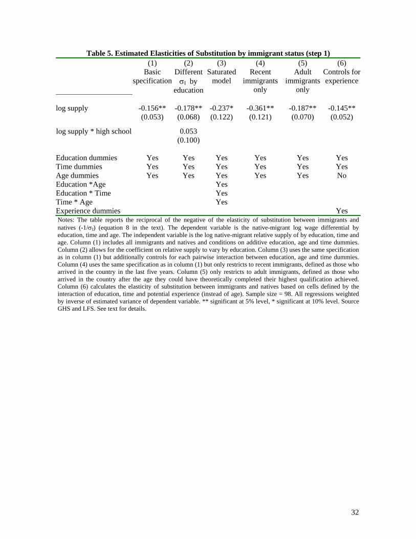
specifications to examine whether our results are sensitive to alternative specifications. Table 5

gives these estimates. Since the dependent variable, the relative native-born wage premia, is

based on regressions using individual data for each cell, we use the reciprocal of the square of the

standard error on these estimated returns as weights and run minimum distance weighted least

squares regressions.

Column (1) reports the basic specification. The model controls for additive age, time and

education dummies. The reported coefficient gives the estimate of the coefficient on the supply of

natives relative to immigrants in the relative wage equation, the negative of the reciprocal of the

elasticity of substitution between immigrants and natives (σI). Under the assumption of perfect

substitutability, the wage gap in each cell should be constant, but the estimates suggest that the

overall native-born wage premium is lower – or below trend – when immigration is lower. The

estimated coefficient is -0.156 and significant at conventional levels, implying an elasticity of

substitution between immigrants and natives of around 6.3. Column (2) interacts the supply term

with the dummy for high school education, allowing for the possibility that elasticity of

substitution could vary by education. Although the point estimates differ across education groups,

the hypothesis that the two coefficients are the same cannot be rejected at usual significance

levels (the difference being 0.053, with a standard error of 0.100).

14

To show that these results are not driven by outliers, in Figure 2 we plot the log native-

immigrant wage (on the vertical axis) against the log native-immigrant supply (on the horizontal

axis) by age, time and education cells. The values are obtained as residuals from regressions of

the relevant variables on additive time, age and education dummies. Each circle represents an

observation in the data, with larger circles implying greater weight. The line in the figure is the

estimated regression line. One can clearly see that regression results are not driven by outliers and

that a similar relationship between wages and supply appears to hold for both those with high

school and those with university education.

One might wonder whether there any particular age-education-year observations which

tend to be on the right or left of Figure 2. As a test, we re-estimate the model with less restrictive

assumptions on the education-age-year dummies. Accordingly column (3) reports an estimate of

model (4) where we include controls for all pair-wise interactions between the age, education and

time dummies. This is a very saturated model and identification of the elasticity of substitution is

only based on the interaction of age, time and education. Even in this highly saturated model, the

negative effect of relative supply remains. The point estimate is -0.237 and significant at the 10%

level.

We next undertake further robustness checks, restricting the definition of immigrants in

the wage cells to be, respectively, recent immigrants (those who arrived in the last five years) and

adult immigrants (those who arrived after finishing their education, age 18 for high school

graduates and age 21 for university graduates).11 Using recent immigrants, column(4) shows that

the estimated coefficient on the supply term is -0.361, implying a low degree of substitution

between natives and recent immigrants, of less than 3. This is intuitive, since it suggests that

recent immigrants largely bear the cost of changes in the stock of immigrants. In column (5) we

report results for older immigrants only. It appears that the wages of these workers are marginally

11 Note we still use all immigrants (whether recent or old, or whether they came to the country as children or adults) to compute supply. This is because information on time since migration is not available in the LFS throughout the period of observation. Care should therefore be used when interpreting these coefficients.

15

more sensitive to changes in the stock of immigrants, though the coefficient is not significantly

different from that in column (1). Finally the estimate in column (6) of the table is based on cells

categorised by the interaction of time, education and potential experience rather than age. The

results are essentially unchanged, with a coefficient of -0.145 and an implied elasticity of

substitution between immigrant and native workers in the order of 6.9

Having ascertained that the estimate of the elasticity of substitution between immigrant

and natives is broadly robust we now estimate the other parameters of the model, namely the

elasticity of substitution between different age and education groups. We replicate the results

from column (1) of Table 5 in the first column of Table 6. The second column reports a new

estimate of this coefficient together with an estimate of the coefficient on the effect of changes in

the relative supply of skills by age and time on the returns to university education (equation(9)).

The estimate of -1/σI remains similar to the one in column (1). The estimated elasticity between

immigrants and native-born falls to around 5 while the estimated coefficient on age-specific

relative labour supply, -1/σA, is -0.108 and statistically significant. This implies an elasticity of

substitution across workers of different ages (σA) of around 10, rather larger than the estimates in

the order of 4.5 found for Britain by Card and Lemieux (2001). Our different sample periods,

sample size, differences in the data used to estimate labour supply, different weights given to

immigrant and native workers and different definitions of education are all likely to explain these

differences. Lastly in column (3) we report new estimates of the effects of the share of natives to

immigrants, the relative supply of university workers by age alongside the estimate of the overall

relative supply of university workers based on equation(11). The estimated coefficient on the

linear time trend used to approximate SBTC is 0.013, so that the graduate to high school wage

gap has grown by around 1.3% a year over the sample period. The data imply an estimated

coefficient on the relative supply of university to high school workers of about -0.172, implying

an elasticity of substitution between university and high school workers, σE, of around 5.8. Again

16

this is larger than the estimate of 2.5 found by Card and Lemieux. The estimate of the elasticity of

substitution between native born and immigrants again remains virtually unchanged.

The estimates so far use population as a measure of labour supply because we believe that

this is a 'more exogenous' source of variation in supply than the employment or hours measures

often used. One can think of our estimates as a ‘reduced-form’. But, there is a danger that our

estimates reflect not just labour demand elasticities but also labour supply elasticities. In order to

present results comparable to the ones generally produced and in order to check for the potential

effect of changes in labour supply on employment, we repeat the exercise using hours of work or

employment as alternative measures of supply and instrument this with the population in each

cell. Table 7 reports two stage least squares results of the regression using hours worked.12 For

the first stage, we find an elasticity of hours relative to the labour supply (at all levels of

aggregation) in the order of one, suggesting an inelastic labour supply curve. Not surprisingly

then, the results based on 2SLS are similar to the estimates in Table 6.

6. Simulating the Effects of Immigration on Relative Wages

In this section we use our results to simulate the effect of changes in the stock and skill mix of

immigrants on various aspects of the wage distribution. To keep things simple we look at only

two summary measures of the wage distribution - the return to education among natives and the

overall native-migrant wage differential. We derive the explicit expressions for the effect of

migration on the wage structure in the Technical Appendix.

In our simulations we consider four cases. First, a 10% rise in the immigrant share in each

cell i.e. a skill-neutral change. Because immigrants are about 10% of employment this is roughly

equivalent to a 1 percentage point rise in the share of immigrants in the economy as a whole.

Secondly, skill-biased changes to the immigrant mix, with a 20% rise in the number of skilled

immigrants and no change in the number of unskilled immigrants. Thirdly, a 20% rise in the

12 The estimates using employment are similar and are available from the authors on request.

17

number of less skilled immigrants and no change in the number of skilled immigrants. Finally we

take the actual change over the period 1975-2005 in the immigrant share relative to the native

share. For our simulations we use the estimates in the final column of Table 6.

The results are shown in Table 8. The first row shows that a 10% rise in the immigrant

share in all cells is predicted to lead to a 2.0% rise in the native-migrant wage differential. This is

what one would expect from a direct reading of the estimates in the final column of Table 6. But

the predicted impact on the return to education among natives is zero – this is what one might

expect from the skill-neutral nature of the change. However the second and third rows also show

that this happens when there is skill bias in the immigrant flows. If all immigrants are skilled the

native-migrant wage differential rises (but only slightly), because of the composition effect –

immigrants are becoming more skilled relative to natives. But there is very little effect on the

return to education among natives. The explanation is that the imperfect substitutability between

natives and immigrants ameliorates the impact on natives.

This can most easily be understood using a simpler model than the one we have used in

which the age dimension is removed from the technology. One can show (see Technical

Appendix) that in this case the change in the return to education among natives in response to a

change in the supply of migrants will be given by:

( ) ( )[ ]tM

tM

IENt

Nt MdsMds

WW

d 22112

1 lnln11ln −⎟⎟⎠

⎞⎜⎜⎝

⎛−−=

σσ (12)

where sMe is the share of the wage bill accruing to immigrants in education cell e. The important

point is that the change in returns is likely to be very small and will be smaller the lower the

degree of substitution among natives and immigrants. It will be small for a number of reasons.

First the term involving the elasticity of substitutions is likely to be small and even ‘perverse’ in

sign given our estimates. Secondly the impact of migration will only have an effect to the extent

that there is a change in the migrants’ skill mix or differences in the wage bill share in the two

education groups.

18

One implication of this is that it is not at all surprising that researchers have failed to

detect any significant effect of immigrants on native outcomes. However this failure does not

mean that there are no economic effects, rather that the effects on groups other than the

immigrants themselves are very small. One can see this also from the fourth column of Table 8

that simulates the effect of the actual changes in immigration over the period 1975-2005 relative

to the case where the immigrant share in each cell remained constant. The prediction is that the

changes have raised the native-migrant wage differential by 0.055 and raised the return to

education by 0.004. This is tiny relative to the 0.15 actual changes over this period.

7. Conclusions

Based on a stylised model of labour demand that allows native-born workers and immigrants to

be imperfect substitutes in production we show how one can, under appropriate identification

assumptions, estimate the elasticity of substitution between immigrants and natives. Given this

framework, the rise in immigration experienced in Britain over the past decades does appear to

have changed the wage structure. It seems that immigration depresses the earnings of immigrants

relative to the native-born, suggesting imperfect substitution between natives and immigrants in

production. When combined with Card and Lemieux's (2001) conclusions (that we confirm even

after the addition of later data) that the return to university education is sensitive to the relative

supply of university graduates, this implies that when immigration has a different skill mix from

the native population this will affect returns to education among natives. Because immigrants are

better-educated than natives, immigration will have reduced the return to education among both

migrants and natives. But, because of the imperfect substitutability between natives and

immigrants and the fact that the immigrant share is still quite low, then the size of this effect will

be small, so it is not surprising that existing studies have failed to find a significant effect on the

labour market outcomes of natives. Our conclusions suggest that the main impact of increased

immigration in the UK is on the outcomes for immigrants who are already here.

19

References

Arellano, M. and Meghir, C. (1992), "Female labour supply and on-the-job search: An empirical model estimated using complementary data sets", Review of Economic Studies, vol. 59(3), pp. 537–559. Bell B., (1997) "The Performance of Immigrants in the United Kingdom: Evidence from the GHS", The Economic Journal, Vol. 107, No. 441 (Mar., 1997), pp. 333-344 Borjas, G., (1987), "Immigrants, Minorities and Labour Market Competition”, Industrial and Labour Relations Review, Vol. 40, No. 3, pp. 382-92. Borjas, G., (1999), "The Economic Analysis of Immigration" Chapter 28, Handbook of Labour Economics, Vol. 3, pp.1697-1760. Borjas, G., (2003), "The Labour Demand Curve is Downward sloping: Re-examining the Impact of Immigration on the Labour market" Quarterly Journal of Economics, Vol. 118, pp. 1335-1374. Borjas G, R.Freeman and L.Katz (1996), “Searching for the Effect of Immigration on the Labour Market”, American Economic Review, May 1996, pp. 246-251. Card, D. (1990), "The Impact of the Mariel Boatlift on the Miami Labour Market", Industrial and Labour Relations Review, Vol. 43, pp. 245-257. Card, D. (2001), "Immigrant Inflows, Native Outflows, and the Local Labour Market Impacts of Higher Immigration", Journal of Labour Economics, Vol. 19(1), pp.22-63. Card, D. (2005), “Is the New Immigration Really So Bad?” Economic Journal, Vol. 115, pp F00-F323, November. Card, D. and DiNardo, J., (2000), “Do Immigrant Inflows Lead to Native Outflows?” American Economic Review, Vol. 90. Card, D., Lemieux, T. (2001), “Can Falling Supply Explain The Rising Return To College For Younger Men? A Cohort-Based Analysis," Quarterly Journal of Economics, Vol. 116(2), pp. 705-746. Chiswick Barry R., Carmel U. Chiswick; Paul W. Miller (1985), "Are Immigrants and Natives Perfect Substitutes in Production?", International Migration Review, Vol. 19, No. 4. (Winter, 1985), pp. 674-685. Dustmann , C. and F. Fabbri (2003), "Language Proficiency and Labour Market Performance of Immigrants in the UK", Economic Journal, 113, 695-717, 2003. Dustmann , C. and F. Fabbri (2005), "Immigrants in the British Labour Market ", Fiscal Studies , vol.26, no.4, pp.423-470, 2005. Dustmann, C. Fabbri, F. and Preston, I., (2005), “The Impact of Immigration on the UK Labour Market”, Economic Journal, Vol. 115, pp F324-F341. Grossman, J., (1982), “The Sustainability of Natives and Immigrants in Production”, Review of Economics and Statistics, Vol. 64, No. 4, pp. 596-603.

20

Katz, L. and K. Murphy (1992), "Changes in Relative Wages, 1963 1987: Supply and Demand Factors", Quarterly Journal of Economics, 107(1), February 1992, pages 35-78. Lalonde, R. and Topel, R., (1991), "Labour Market Adjustments to Increased Immigration", in Immigration , Trade and Labour, (eds.), J. Abowd and R. Freeman, University of Chicago Press. Machin, S., (2003), “Wage Inequality Since 1975”, in R. Dickens, P. Gregg and J. Wadsworth (eds.) The Labour Market Under New Labour: The State of Working Britain, Palgrave-Macmillan Press, London. OECD, (2004), Trends in International Migration, 2004, OECD, Paris Ottaviano, G. and Peri, G. (2005), “Rethinking the Gains From Immigration: Theory and Evidence from The U.S.”, NBER Working Paper No. 11672. Schmitt, J. and Wadsworth, J., (2006), “Changing Patterns In The Relative Economic Performance of Immigrants to Great Britain and the United States, 1980-2000”, Centre for Economic Performance Working Paper No. 1430

21

Data appendix

Definition of education.

We classify the sample into two education categories, university and high school equivalents,

similarly to Katz and Murphy (1992) and Card and Lemieux (2001). We define university

workers as those who left full time education at age 21 or later and high school workers as those

who left full time education between age 17 and 20. Using age left full-time education to define

levels of schooling is not standard practice in Britain so our use of it here needs some

justification.13 Both the LFS and GHS do not always record the qualifications of immigrants

accurately. This is important not just for our purposes but also for more general debates about the

skills of immigrants to the UK.

A large proportion of immigrants in both the LFS and the GHS report holding 'other

qualifications'. Table A1 based on LFS data from 2000-2005 shows that while 6.3% of natives

report holding ‘other qualifications’, 28.8% of immigrants do so. The following two columns of

Table A1 show that the problem is much worse for immigrants who arrived in the UK after the

age at which they left full-time education with 41.8% of this group reporting they hold ‘other’

qualifications compared to 6.0% of immigrants who arrived in the UK before completing full-

time education. The reason for this problem is not entirely clear but there are two likely causes.

First, the qualifications listed in the LFS are British qualifications that do not translate directly

into foreign equivalents and, secondly, it appears that the Office for National Statistics have

deliberately coded all foreign qualifications into the ‘other’ category.

Researchers generally use one of two approaches to deal with the problem caused by

those reporting ‘other qualifications’ – they either code them as missing or as a low level of

qualifications (on the grounds that every conceivable high qualification is covered elsewhere in

the classification). For natives it is likely that results are not very sensitive to this decision rule.

But, for immigrants, it is more of a problem. To code the ‘other’ group as missing is only valid if

13 Bell (1997) in his analysis of immigration to the UK uses a similar definition of skills.

22

they are ‘missing at random’ and to assume they have low qualifications is also problematic. We

can get another idea of the extent of this problem by looking at Table A2 which reports, for each

level of education, the percentage reporting leaving full-time education at or before the age of 16,

17-20 inclusive and 21 or later. The three panels report this information for natives, immigrants

who arrived in the UK before completing full-time education and for those who arrived after. For

natives 93% of those in the ‘other’ category left education by the age of 16 and only 1% after the

age of 21. For immigrants who completed full-time education in the UK the figures are 55% and

20% and for immigrants who completed full-time education outside the UK 20% of the ‘other’

category completed education by the age of 16 and 38% after the age of 21. This suggests that

immigrants in the ‘other category’ are quite well-educated – indeed they seem from Table A2 to

be most similar to those with a degree.

Further information on this point comes from exploiting the panel element of the LFS.

Individuals are in the LFS for 5 quarters and are asked the education question in each quarter so it

is possible that they are coded as ‘other’ in one quarter and something else in another. Table A3

shows the distribution of qualifications among this group. The sample here excludes all who

report being in full-time education or working towards a qualification. One should note that this

group may be dominated by measurement error and is quite small in size. However, 11% of

immigrants in this group report having a degree compared to 0.5% of natives, again suggesting

the immigrants in the ‘other’ group are much better-qualified than the natives.

Table A4 reports the distribution of highest qualification from the 2001 Census (when

such a question was asked for the first time). This question is similar to the LFS question, being

very ‘UK-centric’. But the census does not have a markedly bigger problem with immigrants in

the ‘other’ category or with missing information. And the census suggests a much larger

proportion of immigrants than natives have a university degree.

In short, it is difficult to assign immigrants to the high and low qualification group using

reported levels of qualification. Moreover the highest educational categories are not the same in

23

the GHS and LFS which again hinders the matching process across the two data sets. In order to

circumvent these problems we use instead the variable “age left full time education”, which is

defined consistently across the two data sets.14

Wages

In order to compute wages by cell we use information on weekly earnings of male full time

employees and we drop individuals with weekly earnings below £50 and above £2000 . For the

regressions we group individuals into five year and five year-age cells. We use all the available

data from the GHS spanning between 1973 and 2005.15

To derive measures of the returns to education by immigrant status, age and time we run

separate regressions of the log weekly wages of every individual in each cell (for example native

born workers, born in 1945-1949 observed in 1973-1977) on a dummy for university education, a

linear age term (from 26-32), year dummies (from 1973 to 1977), and a London dummy. We run

this regression only for those with exactly university or high school education (as defined above).

We use a similar procedure to estimate native wage premia for each age-time-education status

cell. Table 3 provides information on returns to education for natives while Table 4 provides

wages of native-born relative to immigrants by skill.

Supply

In order to compute labour supply for each cell, we use the estimated number of individuals in the

population falling in each age/education/migrant status category. In practice we measure the

supply of university graduates as the number of individuals in the sample period that left full time

education at age 21 or later. To compute the supply of high school equivalents we combine the

number of individuals who left full time education between the ages of 17 and 20 together with

14 Despite this, the GHS shows a slowdown in educational attainment based on years of education after 1998 when the questions ascertaining years of education changed from “how old were you when you finished your course” to “how old were you when you finished your continuous full-time education”. 15 There was no GHS from April 1997 to March 1998 and from April 1999 to March 2000.

24

the number of individuals who left full time education at age 16 or under. We weight this second

quantity by the average (over all time periods) of the relative wage of individuals with less than

high school relative to those with exactly high school in each age-nativity group, similarly to

Katz and Murphy (1992) and Card and Lemieux (2001). The wage measure used conditions on a

dummy for London. We use all the available data from the LFS spanning between 1977 and (the

first quarter of) 2006. 16 We present data on the relative supply of natives and immigrants by skill

and on the ratio of the two in table 2.

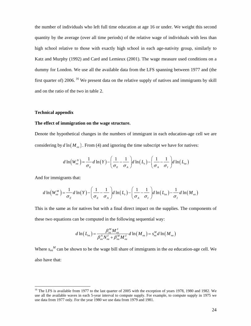
Technical appendix

The effect of immigration on the wage structure.

Denote the hypothetical changes in the numbers of immigrant in each education-age cell we are

considering by ( )ln ead M . From (4) and ignoring the time subscript we have for natives:

( ) ( ) ( ) ( )1 1 1 1 1ln ln ln lnNea e ea

E E A A I

d W d Y d L d Lσ σ σ σ σ

⎛ ⎞ ⎛ ⎞= − − − −⎜ ⎟ ⎜ ⎟

⎝ ⎠ ⎝ ⎠

And for immigrants that:

( ) ( ) ( ) ( ) ( )1 1 1 1 1 1ln ln ln ln lnMea e ea ea

E E A A I I

d W d Y d L d L d Mσ σ σ σ σ σ

⎛ ⎞ ⎛ ⎞= − − − − −⎜ ⎟ ⎜ ⎟

⎝ ⎠ ⎝ ⎠

This is the same as for natives but with a final direct impact on the supplies. The components of

these two equations can be computed in the following sequential way:

( ) ( ) ( )ln ln lnM

Mea eaea ea ea eaN M

ea ea ea ea

Md L d M s d MN M

δ

δ δ

ββ β

= =+

Where seaM can be shown to be the wage bill share of immigrants in the ea education-age cell. We

also have that:

16 The LFS is available from 1977 to the last quarter of 2005 with the exception of years 1978, 1980 and 1982. We use all the available waves in each 5-year interval to compute supply. For example, to compute supply in 1975 we use data from 1977 only. For the year 1980 we use data from 1979 and 1981.

25

( )( )

( )ln

ln lnea ea ea

ae ea ea

aea eaa

L d Ld L s d L

L

η

η

α

α= =

∑∑∑

Where eas can be shown to be the wage bill share of age-group a in education cell e. And finally

that:

( )( )

( )ln

ln lne e e

ee e

ee ee

L d Ld Y s d L

L

ρ

ρ

θ

θ= =

∑∑∑

Where se can be shown to be the wage bill share of education cell e. We use the observed wage

bill shares and estimated elasticities of substitution to compute the changes in wages for each cell

in response to different hypothetical changes in the number and composition of immigrants.

Because we are interested only in summary statistics we need to weight these cell-specific

changes by the employment shares to get the overall changes. When we consider the native

immigrant-wage differential there is an additional composition effect from the change in the skill

mix of immigrants and not just from changes in the wage structure.

Equation (12)

Assuming there is no intermediate age-level in the production function, from the equations above

( ) ( ) ( )( ) ( )1 1ln ln ln lnNe e e

E I

d W d Y d L d Lσ σ

= − +

where ( ) ( )ln lnMe e ed L s d M= and again M

es is the wage bill share of immigrants among the

relevant education group. Taking differences across skills groups of this last equation, this leads

to equation (12) in the text.

26

Figure 1. Immigrant Share in Male Population of Working Age

Source: Computations from LFS various years as described in the text.

27

Figure 2. Native-Migrant Wage Premia and Relative Supply by Age, Time and Education

High School

-.4-.2

0.2

.4.6

-.4 0 .4 .8Supply

University

-.4-.2

0.2

.4.6

-.4 0 .4 .8Supply

The graphs give the log native-migrant wage premia on the vertical axis on the log native-migrant labour supply on the horizontal axis. Both series are obtained as residuals from a regression on additive age, time and education dummies. The line in the figures refers to estimated GLS line. The top graph refers to high school workers while the bottom graph side panel refers to university workers.

28

Table 1. Male Immigrants and Native-Born Men in Britain

1975 1985 1995 2005 Share of immigrants Total 0.081 0.088 0.094 0.119 University 0.128 0.151 0.181 0.201 High School or less 0.078 0.078 0.076 0.093 Share of university graduates Native-born 0.060 0.122 0.154 0.216 Immigrants 0.099 0.227 0.329 0.404 Returns to native-born workers University 0.089 0.100 0.029 0.088 High School 0.243 0.237 0.147 0.129 Returns to university education Native-born 0.123 0.122 0.164 0.244 Immigrants 0.257 0.243 0.296 0.299 Notes. Computations are based on LFS and GHS data as described in the Data Appendix. Returns to education are computed as the regression coefficient of log weekly wages on a dummy for university education, conditional on a quadratic in age and a dummy for London. The returns to native-born are computed as the regression coefficient of log weekly wages on a dummy for university education, conditional on a quadratic in age and a dummy for London. Regressions only include those with a university degree or a high school degree (as defined in the text).

29

Table 2: Immigrant-native-born population ratio by Age, Time and Education

Age 26-30 31-35 36-40 41-45 46-50 51-55 56-60 University 1973-1977 0.151 0.154 0.214 0.141 0.100 0.088 0.116 1978-1982 0.185 0.178 0.224 0.243 0.201 0.206 0.168 1983-1987 0.189 0.182 0.162 0.193 0.202 0.185 0.125 1988-1992 0.203 0.227 0.188 0.176 0.189 0.241 0.246 1993-1997 0.227 0.257 0.252 0.199 0.156 0.209 0.237 1998-2002 0.227 0.274 0.279 0.243 0.198 0.147 0.185 2003-2005 0.276 0.329 0.309 0.272 0.224 0.168 0.139 High school 1973-1977 0.061 0.083 0.099 0.092 0.106 0.081 0.080 1978-1982 0.080 0.064 0.088 0.100 0.097 0.106 0.101 1983-1987 0.076 0.079 0.067 0.082 0.097 0.098 0.108 1988-1992 0.066 0.088 0.096 0.072 0.090 0.111 0.105 1993-1997 0.059 0.074 0.094 0.091 0.068 0.088 0.114 1998-2002 0.083 0.072 0.091 0.098 0.095 0.072 0.093 2003-2005 0.138 0.111 0.088 0.097 0.108 0.108 0.078 Ratio 1973-1977 2.495 1.850 2.156 1.534 0.937 1.637 1.427 1978-1982 2.323 2.772 2.522 2.428 2.062 2.234 1.653 1983-1987 2.493 2.298 2.400 2.344 2.090 2.086 1.143 1988-1992 3.084 2.558 1.953 2.443 2.098 2.369 2.333 1993-1997 3.875 3.440 2.672 2.182 2.273 2.690 2.065 1998-2002 2.722 3.803 3.034 2.483 2.090 2.594 1.985 2003-2005 1.996 2.973 3.509 2.800 2.074 2.386 1.781

Notes. The table reports the ratio between immigrants and natives in the working age population by age, time and education. The top part of the table refers to those with a University degree, the middle part of the table to those with completed High school . Source LFS.

30

Table 3: Returns to University/High School by Age, Year and Immigrant Status

Age 26-30 31-35 36-40 41-45 46-50 51-55 56-60 UK born 1973-1977 0.091 0.120 0.118 0.124 0.116 0.138 0.171 (0.019) (0.028) (0.037) (0.042) (0.048) (0.053) (0.070) 1978-1982 0.054 0.099 0.087 0.152 0.180 0.137 0.155 (0.019) (0.020) (0.030) (0.035) (0.047) (0.054) (0.066) 1983-1987 0.074 0.087 0.156 0.141 0.169 0.051 0.177 (0.022) (0.023) (0.028) (0.039) (0.051) (0.061) (0.090) 1988-1992 0.149 0.177 0.122 0.109 0.075 0.281 0.133 (0.024) (0.025) (0.029) (0.031) (0.047) (0.054) (0.080) 1993-1997 0.169 0.161 0.173 0.135 0.089 0.209 0.151 (0.027) (0.029) (0.032) (0.034) (0.040) (0.054) (0.079) 1998-2002 0.192 0.271 0.243 0.260 0.276 0.240 0.180 (0.032) (0.033) (0.035) (0.039) (0.043) (0.052) (0.086) 2003-2005 0.221 0.285 0.276 0.251 0.275 0.203 0.303 (0.039) (0.041) (0.044) (0.057) (0.054) (0.059) (0.077) Foreign born 1973-1977 0.036 0.175 0.123 0.162 0.455 0.508 0.657 (0.057) (0.063) (0.083) (0.092) (0.104) (0.121) (0.148) 1978-1982 0.056 0.145 0.181 0.079 0.187 0.214 0.409 (0.054) (0.059) (0.072) (0.077) (0.103) (0.142) (0.162) 1983-1987 0.190 0.102 0.345 0.173 0.421 0.149 0.588 (0.072) (0.068) (0.082) (0.097) (0.152) (0.165) (0.185) 1988-1992 0.132 0.153 0.162 0.322 0.438 0.203 0.560 (0.075) (0.081) (0.085) (0.107) (0.139) (0.126) (0.178) 1993-1997 0.034 0.148 0.239 0.528 0.280 0.572 -0.056 (0.086) (0.086) (0.097) (0.094) (0.131) (0.144) (0.223) 1998-2002 0.530 0.417 0.454 0.282 0.328 0.612 0.101 (0.086) (0.088) (0.101) (0.113) (0.135) (0.177) (0.213) 2003-2005 0.157 0.338 0.331 0.354 0.175 0.383 0.428 (0.089) (0.094) (0.108) (0.127) (0.135) (0.161) (0.259)

Notes. Estimated returns to education for immigrants and natives by age and time. Standard errors of the estimated coefficients in brackets. See text for details. Source: GHS.

31

Table 4: Estimated Relative Returns to Native Born by Age, Year and Education

Age 26-30 31-35 36-40 41-45 46-50 51-55 56-60 University 1973-1977 0.107 0.108 0.234 0.203 -0.007 0.066 0.010 (0.046) (0.050) (0.073) (0.075) (0.094) (0.114) (0.136) 1978-1982 0.183 0.075 0.195 0.222 0.226 0.148 0.069 (0.041) (0.045) (0.059) (0.065) (0.090) (0.114) (0.149) 1983-1987 0.025 0.089 0.147 0.181 0.070 0.237 -0.047 (0.054) (0.049) (0.060) (0.073) (0.136) (0.140) (0.156) 1988-1992 0.145 0.203 0.070 0.181 0.026 0.231 -0.137 (0.054) (0.058) (0.060) (0.078) (0.108) (0.103) (0.143) 1993-1997 0.138 0.082 0.013 -0.105 -0.084 -0.004 0.690 (0.066) (0.053) (0.065) (0.066) (0.094) (0.106) (0.180) 1998-2002 -0.080 0.090 0.096 0.060 0.073 -0.103 0.132 (0.062) (0.058) (0.065) (0.073) (0.104) (0.113) (0.138) 2003-2005 0.144 0.072 0.050 -0.022 0.223 0.053 0.214 (0.066) (0.067) (0.083) (0.100) (0.095) (0.119) (0.176) High School 1973-1977 0.052 0.166 0.239 0.237 0.334 0.447 0.496 (0.040) (0.049) (0.059) (0.073) (0.071) (0.070) (0.099) 1978-1982 0.184 0.121 0.289 0.149 0.233 0.225 0.323 (0.040) (0.045) (0.056) (0.059) (0.073) (0.108) (0.091) 1983-1987 0.141 0.104 0.336 0.214 0.323 0.335 0.364 (0.052) (0.054) (0.064) (0.079) (0.087) (0.123) (0.141) 1988-1992 0.128 0.179 0.110 0.394 0.389 0.153 0.290 (0.058) (0.063) (0.067) (0.085) (0.102) (0.095) (0.141) 1993-1997 0.002 0.069 0.078 0.288 0.107 0.359 0.483 (0.063) (0.074) (0.080) (0.077) (0.105) (0.117) (0.177) 1998-2002 0.258 0.229 0.307 0.082 0.124 0.270 0.054 (0.070) (0.075) (0.086) (0.098) (0.102) (0.149) (0.190) 2003-2005 0.080 0.124 0.105 0.081 0.123 0.232 0.340 (0.073) (0.179) (0.086) (0.099) (0.124) (0.133) (0.217)

Notes. Estimated wage differential between natives and immigrants by age and time. Standard errors of the estimated coefficients in brackets. See text for details. Source: GHS.

32

Table 5. Estimated Elasticities of Substitution by immigrant status (step 1)

(1) (2) (3) (4) (5) (6) Basic

specificationDifferent

σI by education

Saturated model

Recent immigrants

only

Adult immigrants

only

Controls for experience

log supply -0.156** -0.178** -0.237* -0.361** -0.187** -0.145** (0.053) (0.068) (0.122) (0.121) (0.070) (0.052)

0.053 log supply * high school (0.100)

Education dummies Yes Yes Yes Yes Yes Yes Time dummies Yes Yes Yes Yes Yes Yes Age dummies Yes Yes Yes Yes Yes No Education *Age Yes Education * Time Yes Time * Age Yes Experience dummies Yes Notes: The table reports the reciprocal of the negative of the elasticity of substitution between immigrants and natives (-1/σI) (equation 8 in the text). The dependent variable is the native-migrant log wage differential by education, time and age. The independent variable is the log native-migrant relative supply of by education, time and age. Column (1) includes all immigrants and natives and conditions on additive education, age and time dummies. Column (2) allows for the coefficient on relative supply to vary by education. Column (3) uses the same specification as in column (1) but additionally controls for each pairwise interaction between education, age and time dummies. Column (4) uses the same specification as in column (1) but only restricts to recent immigrants, defined as those who arrived in the country in the last five years. Column (5) only restricts to adult immigrants, defined as those who arrived in the country after the age they could have theoretically completed their highest qualification achieved. Column (6) calculates the elasticity of substitution between immigrants and natives based on cells defined by the interaction of education, time and potential experience (instead of age). Sample size = 98. All regressions weighted by inverse of estimated variance of dependent variable. ** significant at 5% level, * significant at 10% level. Source GHS and LFS. See text for details.

33

Table 6. Estimated Elasticities of Substitution by Immigrant status, Age and Education Variable Dependent variable: log relative wages

(1) (2) (3) Parameter Native/

Immigrant University/

High School (by age)

University/ High School (aggregate)

Independent variable: log relative supply

(Step 1) (Step 2) (Step 3)

Native-immigrant (-1/σI) -0.156** -0.199** -0.198** by age and education (0.053) (0.065) (0.054)

(-1/σA) -0.108** -0.101** University-High school by age (0.047) (0.048) University-High school (-1/σE) -0.172** (aggregate) (0.054) Time trend S.B.T.C. ` 0.013** (0.003) Education dummies Yes Time dummies Yes Yes Age dummies Yes Yes Yes Immigrant dummy Yes Yes Notes. The Table reports OLS estimates of equations (8), (9) and (10) in the text. The regression in column (1) is the same as reported in Table 5, column (1). See also notes to table 5.

34

Table 7. Elasticities of Substitution by Education, Age and Education (IV estimates)

Dependent Variable 1st Stage 2nd Stage Log employment Log wages (1) (2) (3) (4) (5) (6) Native/

Immigrant University/

High School (by age)

University/ High School (aggregate)

Native/ Immigrant

University/ High School

(by age)

University/ High School (aggregate)

Independent variable: log relative supply

(Step 1) (Step 2) (Step 3)

Native-immigrant 0.938** -0.172** -0.209** -0.204** by age and education (0.081) (0.059) (0.043) (0.071)

1.185** -0.099** -0.095** University-High school by age (0.058) (0.043) (0.44) University-High school 1.186** -0.086** (aggregate) (0.056) (0.028) Time trend ` 0.010** (0.002) Education dummies Yes Yes Time dummies Yes Yes Yes Yes Age dummies Yes Yes Yes Yes Yes Yes Immigrant dummy Yes Yes Yes Yes Method of estimation OLS OLS OLS 2SLS 2SLS 2SLS Notes. The Table reports 2SLS estimates of equations (8), (9) and (10) in the text where employment is instrumented by population. Columns (1) to (3) reports the first stage estimates. Column (4) to (6) report the 2SLS estimates. See also notes to table 6.

35

Table 8. Simulations of the Impact of Immigration on Relative Wages

Log Native-Migrant Wage Differential

Log Skilled-Unskilled Wage Differential

(Natives Only) 10% rise in all immigrants 0.023 0 20% rise in skilled immigrants, No change in unskilled immigrants

0.009 0.001

20% rise in unskilled immigrants, No change in skilled immigrants

0.037 -0.001

Actual change in immigrants relative to natives

0.055 0.004

Notes. These simulations are based on actual wage bill shares in 2005, and the estimates of the elasticities of substitution from the final column of Table 6.

36

Table A1. Highest Qualification of Natives and immigrants, (LFS Data, 2000-2005)

Highest qualification Natives Migrants Migrants Migrants All Left FT Education

before UK arrival Left FT Education after UK arrival

Degree or equivalent 14.3 18.3 12.8 28.0 Higher education 9.0 7.7 6.4 10.1 GCE A-level or equivalent

23.4 13.4 10.0 19.3

GCSE/CSE or equivalent 28.7 12.7 6.4 23.9 Other qualification 6.3 28.8 41.8 6.0 No qualification 17.5 18.4 22.0 12.0 Missing 0.7 0.6 0.6 0.6 Notes. Source: LFS 2000-2005. Sample is individuals aged 16-64 not in full-time education.

Table A2. Highest Qualification and Age Left Full-Time Education of Natives and immigrants, (LFS Data, 2000-2005)

Age lest education Highest qualification 16 or earlier 17/20 inclusive 21 or later Migrants – Left FT Education before UK arrival Degree or equivalent 3.9 23.3 72.9 Higher education 18.3 54.2 27.5 GCE A-level or equivalent 33.3 50.7 16.0 GCSE/CSE or equivalent 36.0 49.7 14.3 Other qualification 20.0 41.7 38.2 No qualification 80.3 17.7 2.0 Missing 58.3 33.4 8.3 Migrants – Left FT Education after UK arrival Degree or equivalent 3.3 12.9 83.8 Higher education 19.1 44.6 36.2 GCE A-level or equivalent 35.9 54.3 9.8 GCSE/CSE or equivalent 54.0 43.6 2.4 Other qualification 55.4 22.7 21.9 No qualification 87.7 11.3 1.0 Missing 61.2 33.1 5.7 Natives Degree or equivalent 10.0 17.6 72.4 Higher education 36.5 42.7 20.9 GCE A-level or equivalent 59.6 37.8 2.6 GCSE/CSE or equivalent 71.6 28.1 0.4 Other qualification 93.5 5.8 0.7 No qualification 97.2 2.7 0.1 Missing 80.6 17.3 2.2 Notes. See notes to Table A1.

37

Table A3. Highest Qualification of Natives and immigrants who report ‘Other’

Qualifications, (LFS Data, 2000-2005) Highest qualification Natives Migrants Migrants Migrants All Left FT

Education before UK arrival

Left FT Education after UK arrival

Degree or equivalent 0.9 11.0 11.5 8.2 Higher education 2.4 6.9 7.5 4.0 GCE A-level or equivalent 32.1 34.9 36.3 27.4 GCSE/CSE or equivalent 39.8 22.3 19.1 40.2 Other qualification 23.5 23.4 24.1 19.8 Missing 1.3 1.4 1.6 0.3 Notes. Sample includes those who report ‘other qualification’ in one quarter and something else in another and excludes those that report being in full-time education or working towards a qualification in any quarter. See also notes to Table A1.

Table A4. Highest Qualification of Natives and Immigrants: Census, 2001 Highest qualification Natives Migrants All Degree or equivalent 19.5 34.9 Higher education 7.1 8.3 GCE A-level or equivalent 39.2 21.8 GCSE/CSE or equivalent 6.1 5.2 Other qualification 25.1 24.3 Missing 3.1 5.4 Source: 2001 Census Sample of Anonymized Records (SARS). Sample is those aged 16-60 inclusive who are not in full-time education and whose country of birth is not missing.