The Impact of Liquidity Regulation Announcements on the CDS Market of Large European Banks

Giorgia Simion1, Ugo Rigoni2, Elisa Cavezzali3, and Andrea Veller4

Department of Management, Ca’ Foscari University of Venice

San Giobbe, Cannaregio 873, 30121 Venice, Italy

Abstract

Following the recent financial crisis, the Basel Committee on Banking Supervision (BCBS) undertook a negotiation process that led up to a liquidity reform package known as the new Basel III liquidity framework. This paper aims to assess the reaction of creditors to announcements by the BCBS on liquidity regulation. Using an event study on Credit Default Swap (CDS) data of large European banks over the 2007-2015 period, we find evidence of a negative CDS market reaction to regulatory events, with CDS spreads widening, indicating that creditors increased expectations of a credit event. Results also show that creditors were less sensitive to liquidity regulation announcements in banks with higher capital and liquidity funding ratios. In contrast, creditors were more sensitive to liquidity regulation announcements in banks with higher bad loans. However, the negative impact of low asset quality is positively moderated by provisions against future expected losses. An important managerial implication of this research is that if banks correctly adjust their asset-liability mix, they could limit potential side effects of the Basel III liquidity regulation. JEL Classification: G21, G28, G14

Keywords: Liquidity Regulation, Credit Default Swap, Event Study, Basel III

1 Tel.: +39 333 8289778. E-mail address: giorgia.simion@unive.it 2 Tel.: +39 041 2348770. E-mail address: rigons@unive.it 3 Tel.: +39 041 2346931. E-mail address: elisa.cavezzali@unive.it 4 E-mail address: andrea.veller@unive.it

2

1. Introduction

This study examines the Credit Default Swap (CDS) market reaction to announcements by the

Basel Committee on Banking Supervision (BCBS) on liquidity regulation, a key milestone in the

new Basel III framework.

Since the financial crisis outbreak in summer 2007, liquidity and funding risk5 started to play a

central role in the field of banking regulation, which until then was almost exclusively focused on

capital ratios (Santos and Elliot, 2012). The lack of a regulation specifically focused on liquidity

proves that this issue was not a major concern by policy makers prior to the crisis. However,

following the turmoil, the common idea that a well capitalized bank was always able to raise funds

became weak: banks, despite meeting the regulatory capital requirements, experienced serious

funding difficulties owing to their excessive reliance on unstable, low quality sources of funding,

erroneous asset-liability management and risky off-balance sheet positions (ECB, 2013).

Consequently, banks became illiquid and unable to meet their debt obligations (i.e. insolvent),

raising significant concerns on liquidity risk.

As a response of the vulnerabilities arose during the crisis, the BCBS undertook a negotiation

process of new, international standards to address the previously underestimated role of liquidity

risk (Calomiris et al., 2012). During this negotiation period, which went on from February 2008 to

June 2015, several amendments were released prior to the final version of the new liquidity reform

package6.

This paper is the first to empirically analyse the impact of the gradual release of official

documents by the BCBS (2008-2015) concerning liquidity regulation on the CDS market of large

European banks, which reflects creditor expectations of default risk. As a first stage, we run an

event study to estimate cumulated abnormal spread changes (CASs) around announcement days,

testing then their statistical significance. As a second stage, we conduct a regression analysis aimed

5 Liquidity risk is the “ability to finance cash outflows at any given point in time” (King, 2013b, p. 4145), while funding risk “refers to a bank’s ability to raise funds in the desired amount on an ongoing basis” (King, 2013b, p. 4145). As it appears evident, these two types of risk are closely interrelated. To lighten reading, we will use the liquidity risk word, assuming implicitly also funding risk. 6 For further details, please see Table 2.

3

at identifying the main determinants of CASs to investigate the heterogeneous response of

investors.

Results show that creditors perceived the introduction of tighter liquidity regulation as reducing

bank probability to survive, with CDS spreads widening. However, as an interesting result, the

effect is mitigated when banks are well-capitalised and with stronger structural liquidity. On the

other hand, the effect is amplified when banks have high bad loan ratios, not covered by loan-loss

provisions.

Surprisingly, while there are several papers dealing with regulatory events and their impact on the

market (e.g., Dann and James, 1982; James, 1983; Allen and Wilhelm, 1988; Wagster, 1996;

Mamun et al., 2004; Yildirim et al., 2006; Armstrong et al., 2010; Bhat et al., 2011; Kolasinski,

2011; Georgescu, 2014), the studies on bank liquidity regulation are scant (Bruno et al., 2015).

Furthermore, among these few pieces of research, to the best of our knowledge, there is no

empirical paper focusing on creditors and examining the complete series of announcements by the

BCBS that led up to the international liquidity standards.

Our paper contributes to prior literature is several ways. From an academic point of view, it

provides new knowledge on a relatively scarcely researched topic. It sheds light on the

interconnection between bank liquidity risk management and credit risk, providing a starting point

for more rigorous formalizations of this important relationship a through theoretical framework.

The relevance of this aspect is particularly important if we consider that liquidity risk and bank

financial stability have been central issues during the financial crisis.

From a practitioner point of view, this paper helps policy markers and bank managers to better

understand how financial institutions would respond to liquidity rules according to their specific

characteristics. This may provide an important tool for banks to mitigate the negative repercussions

of the adoption on profitability (Härle at al., 2010) and business activity (Allen et al., 2012). In

addition, this research supports the impact assessment of Basel III, increasing knowledge on the

international harmonization of liquidity rules.

4

In this framework, examining creditors of European banks is particularly interesting, since they

are excluded from Deposit Insurance Schemes. The lack of protection, together with the hard period

that the banking system was experiencing, should have raised creditors’ concern on bank soundness

and insolvency risk. European financial institutions constitute a peculiar setting in this respect since

they are expected to be most strongly influenced by Basel III (Dietrich et al., 2014) due to their

weaker funding position during the crisis as compared to international peers. Therefore, we expect

creditors of large European banks to be considerably affected by the introduction of the new

liquidity standards.

The remainder of this paper is structured as follows. Next section provides an overview of Basel

III liquidity requirements. Section 3 briefly reviews major studies on this topic. Section 4 develops

the different hypotheses to be tested. Thereafter, section 5 describes the data and methodology used

for the empirical analysis. Section 6 presents the findings. Finally, section 7 concludes.

2. Background on Basel III liquidity requirements

During the financial crisis, the inaccurate banks’ liquidity management and funding structure

became a central issue when liquidity risk clearly arose on banks’ balance sheets (ECB, 2013). In

this difficult period, banks faced significant liquidity outflows and shortages as a result of their

excessive overreliance on highly volatile funding sources (i.e. wholesale market), erroneous

planning of maturity transformation, excessive dependence on low quality assets that quickly turned

to be illiquid and high liquidity risk exposure from off-balance sheet activities. As a consequence,

banks hoarded liquidity for security reasons and reduced their lending activity both to other

financial intermediaries and to the real economy. This contributed to the credit fall, resulting in a

significant drying-up of liquidity funding in several markets (Strahan, 2012). In this context, the

European Central Bank (ECB) adopted extraordinary measures, providing two Longer Term

5

Refinancing Operations (LTROs) 7 with three-year maturity. These non-standard monetary

transactions supported and helped Eurozone banks to meet their debt obligations and liquidity needs

(ECB, 2011).

In light of the inaccurate and ineffective liquidity risk management during the crisis (ECB, 2013),

the BCBS issued in December 2009 a proposal to deal with the increasing concerns on liquidity

risk. This Consultative Document was released after a series of previous attempts to deal with this

issue, which involved other press releases in the period 2008-20098. This proposal framework

aimed to strengthen the financial system stability by increasing the resilience of international active

banks to deal with acute liquidity stress scenarios and promoting the international harmonization of

liquidity risk regulation (BCBS, 2009). To this purpose, the Consultative Document introduced two

separate but complementary standards on banks’ balance sheet: the Liquidity Coverage Ratio (LCR)

and the Net Stable Funding Ratio (NSFR), which address liquidity and funding risk, respectively.

The LCR is designed to help banks in facing short-term liquidity shocks, mitigating the risk of

substantial liquidity outflows due to an excessive dependence on volatile sources of funding. This

standard requires maintaining a minimum amount of “unencumbered, high-quality liquid assets that

can be converted to cash to meet needs for a 30 calendar day time horizon under severe liquidity

stress conditions specified by supervisors” (BCBS, 2010, p. 3). In contrast, the NSFR was

introduced to “promote longer-term funding of the assets and activities of banking organizations by

establishing a minimum acceptable amount of stable funding based on the liquidity of an

institution’s assets and activities over a one-year horizon” (BCBS, 2010, p. 22). This index

mitigates the maturity mismatch between assets and liabilities by promoting the use of stable, long-

term funding sources and penalizing instead short-term wholesale funding, one of the central issues

of the financial crisis.

Following the proposal, in December 2010 the final version of the new liquidity standards was

7 In this respect, the European Central Bank (ECB) conducted two three-year Longer Term Refinancing Operations (LTROs), characterized by fix rate and full allotment: the first on 21st December 2011 that introduced in the market €489 billion to 523 credit institutions and the second on 29th

February 2012 that provided €529 billion. 8 Further details will be provided in paragraph 5.2.1..

6

released by the BCBS, in which the LCR was partially relaxed and the NSFR maintained

substantially unchanged. Despite some revisions on the ratios, the reaction of the banking

community to this press release was of enormous dissent. In that period, European banks were

experiencing the terrible repercussions of the sovereign debt crisis and perceived the adoption of the

liquidity requirements as punitive. Overall, the document received strong criticisms, especially

among European banks, which compared to their international peers (e.g. US and Japan) were

clearly in a weaker funding position and thus less prepared to fulfil the new standards.

Thereafter, a series of revisions and adjustments were made by the BCBS as a response to banks’

comments and impact assessments. This resulted in a softening up of the initial version of the

guidelines and the gradual introduction9 of the liquidity standards to avoid, or at least contain,

potentially negative effects on credit market (Bruno et al., 2015). In light of this, additional

amendments were released that went on subsequent years and that ended in June 2015 with the

release of the final document on the NSFR introducing some minor revisions on the index. Relying

on the official publications by the BCBS, the LCR was introduced in January 2015 for a minimum

amount of 60 per cent and will gradually increase until 2019 (ECB, 2013), year in which the

minimum level will reach 100 per cent. The NSFR instead will be introduced in January 2018,

requiring bank to maintain a minimum level of 100 per cent.

Overall, the new Basel III liquidity requirements are expected to increase banks’ liquidity buffers,

lower maturity imbalances, contain the interconnection of financial markets and, last but not least,

reduce systematic liquidity risk (ECB, 2013).

Importantly, all member nations of the BCBS10 have to introduce in their respective countries the

liquidity standards. Bank failure to comply with these reforms would incur into financial penalties

and in the worst case the cancellation of the banking licence.

9 This concerns specifically the Liquidity Coverage Ratio (LCR). 10 The Member Nations represented on the Basel Committee of Banking Supervision (BCBS) are Belgium, Canada, France, Germany, Italy, Japan, Luxembourg, the Netherlands, Spain, Sweden, Switzerland, the United Kingdom, and the United States. For further details, see <http://www.bis.org/bcbs/membership.htm>.

7

3. Literature Review

3.1. Bank Regulation and Market Effect

The market reaction arising from changes in bank regulation have been studied by several

researches and can be dated back to the 80s, when the first single-country papers on this field

appeared in the literature. These studies mainly focused on the US market, exclusively analysing

equity investors.

In this respect, Dann and James (1982) examined shareholders’ wealth effects of three events

occurred in the period 1973-1978 concerning the removal of interest rate ceiling on deposits. By

analysing a sample of US saving and loan (S&L) institutions, they found a significant reduction in

the market value of stocks following the rule change.

Thereafter, James (1983) undertook a similar study, extending the analysis to commercial banks in

US, and found significant intra-industry heterogeneous effects owing to ceiling changes.

Other deregulations, following to these rule reforms, lead to the 1980 Depository Institutions

Deregulation and Monetary Control Act (DIDMCA) analysed by Allen and Wilhelm (1988). The

authors found a substantial impact of the DIDMCA passage on the competitive structure of banks.

Institutions that were member of the Federal Reserve System (FRS) resulted to profit more from the

passage as compared to non-FRS institutions.

The first multi-country study, shifting to a more international environment, is that of Wagster in

1996. He conducted an event study to examine how the competitiveness of international banks was

affected by the introduction of the 1988 Basel Capital Accord. His empirical results reveal that the

capital regulation failed to eliminate the cost-funding advantages of Japanese banks, thus missing to

reduce the competitive inequalities among nations within this sector.

Since the beginning of the 21st century, a series of management studies started to examine the key

events leading to the introduction of the US Gramm-Leach-Bliley-Act (GLB)11 in 1999. Among

11 “The GBL Act repealed the Glass-Steagall Act of 1933 and the Bank Holding Company Act of 1956 and allowed banks, brokerage firms, and insurance companies to merge” (Mamun et al., 2004, p. 333).

8

others, important are the works of Mamun et al. (2004) and Yildirim et al. (2006) that found a

significant reduction in the systematic riskiness of the financial industry around the event days of

the passage, concluding that this sector has positively benefitted from the GLB Act.

In addition to the US context, more recent research on bank regulation and investors’ reaction has

started to examine also the European market and banking system. To this regard, Armstrong et al.

(2010) analysed the series of announcements (2002-2005) related to the adoption of IFRS standards

in the European stock market. They showed that banks with lower pre-adoption information quality

reacted positively to the standard, consistent with the expected rise in the quality of accounting

information.

Thereafter, in the face of the 2007-2008 turmoil and the resulting weakening of the financial

system, which led shareholders and creditors to question about bank solvency, research started to

examine also bondholders. This was motivated by the fact that creditors became increasingly

exposed to lose money and thus more sensible to credit risk as compared to the pre-crisis period.

Consequently, this figure became object of analysis in several related researches.

Among these studies, Georgescu (2014) examined how credit and equity market participants

reacted to the relaxation of fair value accounting in 2008. By conducting an event study on stock,

bond and CDS data on European banks, he discovered that bondholders and shareholders display

heterogeneous responses.

Another recent paper, which extended previous works by looking at both credit and equity market

participants, is the paper by Bhat et al. (2011). The authors investigated how bond and stock prices

responded to a series of announcements that led up to the mark-to-market accounting rule change

and found a positive bond and stock price reaction surrounding the event days.

3.2. Government Interventions and Market Effect

Following the outbreak of the crisis, other research has evaluated the impact of government

interventions aimed at increasing stability of the financial system and restoring investor confidence

9

in the market. Regulation and government interventions are actions that are not on the same level,

however the studies display the reaction of creditors (and also shareholders) to safeguard measures,

which is object of interest in this research.

Veronesi and Zingales (2010) carried out an event study to analyse the costs and benefits of the

US government intervention announced in October 2008, according to which the nine largest US

banks were planned to receive huge capital injections. They found that the government intervention

significantly raised banks’ claim, benefiting mostly bondholders, which gained around $121bn.

Despite this increase in value, the plan involved a substantial redistribution of wealth at the expense

of taxpayers that lost between $21–$44 bn.

Another interesting paper is the one by King (2009). The author examined how creditors and

shareholders reacted to the introduction of rescue packages for six countries in the period 2008-

2009. To this purpose, first he carried out an event study at the country-level to assess the average

effect of the announcements associated with the introduction of the rescue package and second at

the bank-level, by differentiating institutions according to the type of support received (e.g. capital

injection, asset purchase etc.), with the goal to investigate potential heterogeneous effects. Overall,

he concluded that government interventions mainly favoured bondholders at the expense of

shareholders for almost all countries under examination.

In addition to the previous work, King (2013a) conducted another related study with the aim to

analyse potential contagion and competition effects following the government bailout measures

occurred in 2008. His results, from a sample of 63 banks belonging to five countries, show a strong

contagion effect for bondholders, expressed by a reduction in CDS spreads for both the banks

subject to the intervention and their foreign competitors. In contrast, a mixed effect was found for

shareholders.

In sum, research on bank regulation and market effect emerged in the 80s in the US market,

mainly focusing on shareholders. Thereafter, studies shifted to the European setting, starting to

recently examine the figure of bondholders, which became increasingly expose to bare losses

10

following the crisis. Furthermore, other related studies examined the role of government

intervention and its effect on credit and equity market participants.

Overall, the literature highlights significant redistribution of resources owing to rule changes. The

purpose of this paper is to analyse how creditors responded to the introduction of the new liquidity

standards. For this reason, we next turn the attention to the studies that examined the effect of the

Basel III liquidity framework.

3.3. Recent Studies on Basel III liquidity standards

One of the central aspects discussed in the literature is the impact of the new liquidity standards on

bank asset-liability management, since long-term funding12 is costly and holding more high quality

liquid assets yields low returns (Dietrich et al., 2014). King (2013b) analysed a sample of 549 banks

in 15 countries to investigate their compliance with the NSFR at the end of 2009 and identify the

best procedure to meet the index in case the ratio falls below the minimum threshold. By analysing

various strategies, the author found that the most cost-efficient proceeding is to increase the

maturity of wholesale funding and the amount of high-rated securities, thus affecting interest spread

between assets and liabilities. However, this strategy is expected to narrow down net interest

margins by an average amount of 75 basis points.

As a result of the downward pressures on lending margins, some studies (e.g. Härle at al., 2010)

foresee a reduction in the return on equity (ROE) index, a standard measure of bank profitability.

Other research instead does not confirm this negative relationship, illustrating the potential benefits

of the adoption. Dietrich et al. (2014), examining the drivers and outcomes of the NSFR prior to its

introduction (1996-2010), show that the funding ratio does not significantly impact a set of bank

profitability variables. The authors interpret this finding as evidence that there are well-balanced

business models able to raise profits despite the disadvantages of the higher short-term funding

costs related to the implementation of the index.

12 Under the assumption of a positively sloped yield curve.

11

The aspect of business models is in fact another relevant topic analysed by researchers, who

started looking at banks not merely as a portfolio of assets and liabilities but as an entity able to

adjust its activities to the new liquidity regime. Allen et al. (2012) claim that the impact of the Basel

III reform could be less harmful than the banking industry fears. However, in order to have such a

favourable result, substantial structural adjustments are required, which represent a significant

challenge for financial institutions in the transition period towards the adoption. The authors predict

that bank business models will shift toward a liability-oriented assets management, primarily

focused on stable and long-term funding sources. Importantly, they highlight that bank failure to

implement the necessary changes may make the cure worst than the disease, increasing

substantially bank costs. Overall, it is generally agreed that banks with a more diversified funding

structure, as is the case of investment banks, are more likely to experience difficulties in meeting

the liquidity standards since they generally rely on funding sources (e.g. wholesale debt) penalized

by Basel III criteria (Allen et al., 2012; Dietrich et al., 2014).

In contrast to prior research, our paper takes a different view examining the short-term effect of

liquidity regulation on the financial market. An assessment of the long-term impact would be hard

to implement accurately since the liquidity standards have not been fully adopted yet and can only

be computed for a very short time. Therefore, only an event study approach can be used to examine

how creditors perceived that the regulation would affect bank soundness. Moreover, the market

analysis can capture all public information conveyed to investors and examine the overall effect of

liquidity regulation, without making simplifying assumptions or conjectures on bank operating

reactions.

To the best of our knowledge, there is only one working paper by Bruno et al. (2015) that examine

the market effect of Basel III. The authors found a negative share price reaction around the days

leading to the liquidity reform, suggesting that shareholders believe that the adoption decreases

bank profitability. In addition, they reported a heterogeneous market reaction based on bank country

of origin and specific bank characteristics. However, Bruno et al. (2015) did not consider creditors,

12

which might have different incentives as compared to shareholders. The issue is particularly

important since creditors in Europe are excluded from Deposit Insurance Schemes. Therefore, given

the vulnerabilities emerged during the recent financial crisis, which strongly hit European banks,

the lack of protection schemes is likely to have raised their concern on bank soundness, supporting

the idea of a significant reaction to the liquidity rules.

Overall, this research is the first empirical analysis that aims to assess creditor reaction, proxied

using changes in CDS spreads, to regulatory announcements that led up the liquidity portion of the

new Basel III package.

4. Hypothesis development

To the extent that liquidity regulation provides new information to investors, we expect a

significant market reaction to the announcements. A positive reaction would suggest that creditors

viewed the introduction of the liquidity rules as reducing the risk of default for banks, with the CDS

spread narrowing around the event days. A negative reaction would instead show that creditors

perceived the standards as increasing the risk of default, with the CDS spread widening following

the regulatory events.

Several studies in the literature support the former hypothesis of a positive response. The

regulation is in fact designed to reduce the contagion risk of liquidity shortages (BCBS, 2010),

improving banking system soundness and reducing bank credit risk. In support of this argument,

Dietrich et al. (2014) show that high NSFR banks display lower earnings volatility. Hong (2014)

find a negative relationship between NSFR and bank failure for a sample of US financial

institutions, although no similar effect is reported for the LCR. Finally, Banerjee and Mio (2014)

highlight the contagion-limiting effect of liquidity rules. Specifically, they document that a tougher

liquidity regulation decreases bank interconnectedness, mitigating the transmission of shocks and

strengthening the stability of financial institutions.

13

The above research supports the beneficial effects of liquidity regulation on bank soundness and

explains why creditors may respond positively reducing their perceived default risk.

Despite these arguments, other related research predicts a negative reaction. This view is mainly

driven by the high cost and potential “dark side” effects of holding liquid assets, as required by

Basel III. Myers and Rajan (1998) illustrate that bank with more liquid assets have a higher value in

liquidation for creditors but they are also more exposed to unfavourable behaviour by borrowers

that may act against creditors’ interests. Moreover, as supported by some research findings, the low-

yielding liquidity and higher cost of long-term funding may substantially harm bank profitability

(Härle at al., 2010; King, 2013b). If creditors view the new liquidity standards as detrimental for

bank soundness, they should respond negatively increasing their perceived default risk following

the regulatory events.

Beside understanding the overall effect of the regulation, it is reasonable to expect that not all

financial institutions will respond equally. Because the liquidity rules are first realized at the bank

level (BIS, 2016), it is worth understanding whether bank-specific characteristics, especially the

risk dimensions closely related to the liquidity standards, influence the CDS market reaction.

Specifically, our testable hypotheses about the heterogeneity of creditor response are the

following:

H1. Creditors of banks with higher liquidity funding ratios react positively to liquidity regulation

announcements.

The idea that banks with liquid assets and stable funding sources better withstand with liquidity

shocks stands at the heart of the liquidity reform (BCBS, 2010) and is further confirmed by prior

literature (Cornett et al., 2011). Research on the recent crisis supports this argument, highlighting

that bank liquidity funding structure is a central factor in explaining bank default risk and showing

that financial institutions with stronger structural liquidity in the pre-turmoil period were less likely

14

to fail afterward (Bologna, 2001; Vazquez and Federico, 2012). Importantly, holding more liquid

assets also improves bank creditworthiness, increases access to external funds and reduces bank

funding costs (Sironi, 2003). The above arguments match the intuition behind the implementation

of the LCR and NSFR. We therefore believe that bank characterized by a stronger funding system

and more liquid assets are more likely to fulfil the new standards. As a consequence, their creditors

should be less sensitive to the introduction of stricter liquidity regulations.

H2. Creditors of banks with higher capital ratios react positively to liquidity regulation

announcements.

Whereas examining the exposure of well-capitalized banks to regulatory policies on liquidity is a

relatively scant research topic13, several studies tested the impact of leverage on bank CDS spread

and cost of debt (Flannery and Sorescu, 1996; Sironi, 2003; Di Cesare and Guazzarotti, 2010). It is

commonly agreed that higher capital ratios lower leverage, decreases funding costs, thereby

reducing the probability of bank default. We therefore expect that highly capitalized banks are in a

better funding position to meet the tighter liquidity standards without facing financial distress.

There are several reasons that support such an argument: (1) capitalized banks are less likely to

suffer from increased funding costs due to the adoption since we presume that they have a more

resilient and stable funding structure, (2) they are perceived as less risky by investors and therefore

have more easily accessible funds (Ratnovski, 2013), and (3) they automatically increase bank

NSFR through more equity14 so that they have less need for costly balance sheet adjustments.

Overall, we predict creditor reaction to be smaller for bank with higher capital ratios because

investors, anticipating the benefits of lower leverage, reduce expectations of a credit event.

13 To the best of our knowledge there is only one paper by Dietrich et al. (2014) that analysed the determinant of NSFR and found a positive relationship between bank capital level and the liquidity ratio. 14 Equity stands at the numerator of NSFR and has a ASF-factor of 100%.

15

H3. Creditors of banks with higher bad loans react negatively to liquidity regulation

announcements. This effect is positively moderated by a bad loan coverage ratio.

Low-quality asset banks are clearly in a weaker position to accommodate the new standards. Bad

loans are in fact penalised by Basel III criteria as they automatically lower the NSFR15 (BCBS,

2014c) and implicitly harm the LCR, not being by definition High Quality Liquid Assets (HQLA).

Hence, these banks are expected to face higher pressures to adjust their asset-liability portfolio

composition and greater uncertainty on future performance. A recent study by Hong et al. (2014)

confirm that banks with low asset quality have higher credit risk and are prone to default. Because

they are perceived as riskier, they also face higher funding costs and fund-raising problems, thus

making the adjustment process toward the adoption more challenging. Overall, creditors of banks

with higher bad loan ratios are expected to raise their perceived default risk following the regulatory

events. Nevertheless, we believe that this effect is positively moderated by the amount of

allowances set aside by banks to cover non-performing loans. Indeed, the risk of a credit event

decreases as the cushion against expected losses increases. If investors correctly evaluate this

information, the negative reaction should be less pronounced for banks with a higher bad loan

coverage ratio.

5. Data and Methodology

5.1. Data

For the purpose of this study, we use the daily change in the CDS spread as proxy for the effect on

bank creditors. A growing body of research supports this choice, measuring debtholders’ reaction

employing CDS data instead of bond data (King, 2009; Veronesi and Zingales, 2010; Andres et al.,

2016). This provides several advantages. First, banks generally issue different types of bonds,

which in turn have different characteristics (e.g. maturity and liquidity). Combining them to assess

15 Non-performing loans are assigned a RSF-factor of 100%.

16

the overall impact of an event may be challenging. Contrary to the bond market, only one derivative

contract is required for each bank. Second, CDS contracts are generally more liquid than bonds

(Veronesi and Zingales, 2010) and therefore provide much more reliable data. Finally, whereas

bond spreads incorporate information not related to default risk, CDS spreads are a direct measure

of credit risk.

For these reasons, individual bank CDS contracts are selected from Markit Ltd., one of the most

reliable and widely used data provider on CDS, which employs rigorous data cleaning proceedings

to construct their composite spreads. For the period from July 2007-June 201516, we gather daily

observations on 5-year CDS contracts17 denominated in Euro and written on senior unsecured debt

with mod-modified restructuring clause18.

Banks are selected as the largest European financial institutions according to asset size. We first

look at the list of significant banks under the Single Supervisory Mechanism (SSM) Framework

Regulation. This allow us to classify, based on bank’s size, the most representative financial

institutions under the SSM. Then, we integrate the above list with that of the remaining countries,

which do not participate in the SSM: Denmark, Norway, Sweden, Switzerland and UK.

To be included in the final database, bank CDS must satisfy a series of liquidity criteria. We

arbitrarily select the threshold according to prior research (Andres et al., 2016), with the main goal

to get a correct balance between the need of having a representative dataset and reliable

observations. The selection criteria we apply are the following: CDS data have to be observable for

each day of the event window, for at least 50 per cent of the trading days of the estimation

window19 and the percentage of zero spread change should not exceed 50 per cent of the estimation

window.

16 Not all banks have observable data from the whole investigated period. More in details, Deutsche Apotheker- und Ärztebank EG has available data from September 2007 until September 2014. DNB Bank ASA from November 2011. DZ Bank AG Deutsche Zentral- Genossenschaftsbank has observable CDS until September 2014. Erste Group Bk AG from August 2008. Eurobank Ergasias, S.A. from August 2008. FCE bank until September 2014. Lloyds Bank Plc until October 2013. Piraeus Bank SA until September 2014. Finally, Permanents TSB Plc from July 2007. 17 5-year CDS contracts are the most liquid derivative contracts, commonly used in prior related research. 18 CDS derivative contracts are regulated by the International Swap and Derivative Association (ISDA) and are traded Over the Counter (OTC). The ISDA determines the restructuring clause and which form of bank debt restructuring represents a credit event. CDS on European banks currently follow the Modified-Modified Restructuring convention. 19 These two time intervals will be defined in paragraph 5.2.2.

17

The data collection process result in an unbalanced20 panel of 50 banks from 15 European

countries, i.e. Austria, Belgium, Denmark, French, Germany, Greece, Ireland, Italy, Norway,

Portugal, Spain, Sweden, Switzerland, the Netherland and the UK. Table 1 shows the banks of this

study together with their number of observations.

For the same time period, we also collect data on the iTraxx Europe 5-year index21, our proxy for

the market portfolio. This index is made up of the most liquidity 5-year CDS contacts of European

financial and non-financial institutions.

As a last step, we gather from Bankscope accounting information on bank consolidated financial

statements to construct bank-specific variables.

[insert Table 1 here]

5.2. Methodology

5.2.1 Event dates

We define an event date as the exact day on which new information regarding bank liquidity

regulation becomes available on the market. In line with this statement and previous studies on

regulatory events (Yildirim et al., 2006), each date corresponds to the release of an official

document by the BCBS concerning liquidity regulation22. If the publication occurred on public

holidays, the first available trading day is selected as event date.

To identify the events of this study, we apply the following procedure. Based on the public

information available on the BIS23 website, we consider all the documents in the BIS section

labelled “Basel Committee - Liquidity”24, which includes all publications of the BCBS concerning

liquidity since 1992. Thereafter, we refine the above list by selecting only the proposals,

20 The number of financial institutions changes among events and thus through time as some of them did not satisfy the requirements for each of the 12 events under examination. 21 Specifically, we used the series 23, version 1 of the iTraxx Europe 5-year index. 22 If two documents on liquidity regulation are released on the same day, the two publications belong to the same event. 23 BIS stands for Bank for International Settlements. 24 See <http://www.bis.org/list/bcbs/tid_128/index.htm>.

18

amendments and final documents on liquidity regulation exclusively related to the Basel III

framework. Through this process, we identify 11 events in the period 2008-2015.

We further examine all the BCBS press releases available on the BIS website25 in order to check

that significant publications on liquidity are not missing in the analysis. This lead us to add an

additional event concerning the release of an Annex in July 2010, which contains key agreements

on the liquidity reform.

To complete the selection of event dates, we carry out a research on Lexis Nexis Academic to

verify that the events we focus on really conveyed new information to the public, thus making

investors informed of the liquidity rules. This proceeding also allows us to examine potential

anticipatory effects. More in detail, we conduct a search on major international magazines (e.g.

Financial Times, International New York Times, International Herald Tribune) over a span of a

week before and after each event, using a wide rage of keywords26 to assess international media

coverage of the Basel III liquidity framework. This process confirms our selection and does not

show the release by the press of information on the events prior to their official announcements by

the BCBS.

Overall, we select 12 events related to the new liquidity regulation and covering the period

between February 2008 and June 2015. Table 2 defines each event date and provides a brief

description.

Finally, each author independently categorizes the events in two classes: (1) those that tightened

the liquidity requirements and (2) those that loosen them conditional to prior events and disclosed

information. Table 3 document our final event categorization.

[insert Table 2 here]

[insert Table 3 here]

25 See <http://www.bis.org/list/press_releases/said_7/index.htm>. 26 Specifically, we rely on the following main keywords: liquidity regulation, Basel III, liquidity risk, funding risk, NSFR, LCR, liquidity and funding management, Basel Committee, Bank for International Settlements.

19

5.2.2. Event study

To investigate creditor reaction to regulatory events on liquidity, we adopt an event study

methodology. This technique allows quantifying the impact of liquidity regulation announcements

on bank CDS spreads.

Based on prior literature (MacKinlay, 1997), we estimate abnormal CDS spread changes (ASC)

following a series of steps. We first compute spread changes, which reflect the interday variation in

the premium, by making the difference in the logarithm of the CDS spread between two

consecutive trading days. Formally, this can be represented as:

∆𝑆#,% = 𝑙𝑛(𝑆#,%) − 𝑙𝑛(𝑆#,%-.) (1)

where Si,t and Si,t-1 is the spread level (in basis points) at time t and t-1, respectively.

The choice to use the difference in the logarithm instead of the absolute difference is driven by the

fact we expect a market reaction that is proportional to banks’ initial level of credit risk. In such

circumstances, the absolute difference is considered as less appropriate measure (Andres et al.,

2016).

Thereafter, we define abnormal changes in CDS spreads as the difference between the realized

and the normal spread change over the event window:

𝐴𝑆𝐶#,% = ∆𝑆#,% − 𝐸[𝛥 𝑆#,% |𝛺%] (2)

where 𝐴𝑆𝐶#,% , ∆𝑆#,% and 𝐸[Δ 𝑆#,% |Ω%] correspond to the abnormal, realized and normal spread

change for contract i at time t, respectively. Note that the normal spread change, i.e. the spread that

would be observed if the event did not occur, is conditioned by past CDS changes, identified by the

information set 𝛺% at time t.

While the realized spread change is computed using equation (1), the normal spread change is

obtained applying a standard market model (MacKinlay, 1997)27. This is expressed by the following

equation:

27 Note that the spread change of the market index is obtained by applying the same computation used for the CDS spread changes. Specifically, the spread change of the market index is set as the difference in the logarithm of the market index spreads between two consecutive trading days.

20

∆𝑆#,% = 𝛼# +𝛽#𝛥𝑆#<=>?,% + 𝜖#,%

𝐸 𝜖#,% = 0 𝑉𝐴𝑅 𝜖#,% = 𝜎EFG (3)

where 𝛥𝑆#<=>?,% is the spread change of the CDS market index, proxied by the iTraxx Europe 5-

year index, and 𝜖#,% is the error term. We then estimate via an OLS28 regression the parameters 𝛼#,

𝛽# and 𝜎EFG of equation (3) over a 150-day estimation window, ending 3 day before the

announcement.

Finally, according to equation (2), we compute the abnormal spread change (ASC) of contract i on

the event date t as follows:

𝐴𝑆𝐶#,% = 𝛥 𝑆#,% − 𝛼H +𝛽H𝛥𝑆#<=>?,% (4)

In order to capture potential anticipated or postponed market reactions, we focus on the following

event windows: 5-day (-2; +2), 3-day (–1; +1), 2-day (0; +1) and one-day (0; 0)29. Cumulative

abnormal CDS spread changes (CASs) for these event windows is calculated by adding abnormal

CDS spreads, obtained via equation (4), within the event period.

After the computation of CASs for each bank-event combination, we test the hypothesis of a

market reaction statistically different from zero using several parametric and non-parametric test

statistics. Because the introduction of the liquidity standards resulted from a series of press releases

that occurred over several years, we draw our inference from the analysis first on the single events

and second on all 12 events taken together.

With reference to the analysis on the single events, we run the Boehmer et al. (1991) test, which is

robust to event-induced volatility, the widely used Wilcoxon sign rank (1945) test and finally, as a

robustness check, the recent generalized sign test proposed by Kolari and Pynnonnen (2011), which

is robust to return serial correlation, event-induced volatility and cross sectional correlation.

With reference to the analysis on all events, we construct equally-weighted CDS portfolios since

they are free from potential cross-sectional correlation due to the clustering of events (MacKinlay, 28 Before running the model, we check that the OLS assumptions were satisfied. Specifically, we run the Box–Pierce, Lilliefors (Kolmogorov-Smirnov) and Breusch-Pagan tests. As some regressions resulted to have heteroskedasticity issues, we use the hsk-wls procedure for heteroskedasticity correction of the estimates. 29 As a robustness check, we also include other event windows.

21

1997). Because we recognize some events as tightening and loosing liquidity regulation, in the

same spirit of Armstrong (2010), we multiply by -1 the announcements associated to weaker

liquidity rules. This technique allows us to correctly estimate the overall CDS market reaction to

tighter liquidity regulation. The intuition behind it is related to the fact that a positive reaction to

events that reduced the requirements suggests that creditors benefitted from loosing regulation.

Therefore, it would be inappropriate to aggregate the raw CASs for both event categorizations.

We run two test statistics on CDS portfolios, the standard t-test and the Wilcoxon sign rank

(1945) test.

Finally, as a robustness check, we estimate CASs adopting a factor model, which includes the

most important determinants of CDS changes identified by prior literature (Collin-Dufresne, 2001;

Ericsson et al., 2009)

5.2. Regression analysis

As a second step, we examine the determinants of heterogeneous market reaction to regulatory

events by running the following regression:

𝐶𝐴𝑆#,I%J%K = 𝛼 + 𝛽L𝐵𝐴𝑁𝐾#,LL + 𝛾<𝑡𝑖𝑚𝑒_𝑑𝑢𝑚𝑚𝑦< + 𝜆I𝐶𝑂𝑁𝑇𝑅𝑂𝐿𝑆#,I +I< 𝜀#,I

%J%K (5)

where the dependent variable is the cumulative abnormal spread change for bank i and event j

over the event window (𝑡.; 𝑡G) and 𝐵𝐴𝑁𝐾#,L is a vector of bank-specific accounting variables. In

line with prior literature (Ricci, 2015), for each event we associate the latest available accounting

variable30. Finally, we include a set of time dummies to capture different phases of the financial

crisis (𝑡𝑖𝑚𝑒_𝑑𝑢𝑚𝑚𝑦<) and some controls (𝐶𝑂𝑁𝑇𝑅𝑂𝐿𝑆#,I).

With reference to bank capitalization, we consider the TIER1 regulatory capital ratio, i.e. the ratio

between regulatory bank equity capital and total risk-weighted assets. According to our hypothesis,

we expect that higher bank capital ratios have a positive effect on creditor reaction to regulatory

announcements, decreasing their expectations of a credit event. Therefore, H1 is confirmed if the

30 For example, considering an event occurred in 2008, we associated accounting variables measured from the bank annual report of 2007.

22

TIER1 coefficient is negative and statistically significant at least at the 10% confidence interval,

reflecting a narrowing in CDS spreads.

With reference to bank liquidity, we construct two indicators: the Liquidity Coverage Ratio (LCR)

and the Net Stable Funding Ratio (NSFR). As previously stated, the actual ratios cannot be

accurately obtained from annual reports: we therefore derived reasonable proxies from Bankscope

datase. More in detail, the former variable (LCR) is defined as liquid assets31 to deposits and short-

term funding, while the latter one (NSFR) is defined as the ratio of equity32 and long term funding33

to total year-end assets34. Consistently with our hypotheses, we assume creditors in banks with

higher liquidity funding ratios to react positively to liquidity regulation announcements, i.e. they

decrease their perceived default risk more than investors in less liquid banks do. Consequently, H2

is confirmed if the LCR and NSFR coefficients are statistically significant, with a negative sign.

With reference to asset quality, we construct the ratio of impaired loans to gross loans (NPL_GL)

and the ratio of loan loss reserves to impaired loans (LLR_NPL) to capture the moderating effect of

bad loans coverage. We expect creditors of banks with higher bad loans ratios to respond negatively

to liquidity regulation announcements, increasing their perceived default risk. However, we believe

that this effect is positively moderated by the amount of provisions covering expected losses. In line

with this statement, H3 is confirmed if the coefficients of the NPL_GL and the interaction term

between NPL_GL and LLR are significant, with a positive and negative sign, respectively.

Beside our interest variables, we include three time dummies: GLOBAL indicates the global crisis

period (15/09/2008-01/05/2010), SOVEREIGN captures the sovereign debt crisis (02/05/2010-

21/12/2011) and finally post_LTRO reflects the period after the two Longer Term Refinancing

Operations (from 22/12/2011) by the European Central Bank (ECB) that provided huge capital

injection to financial institutions.

31 Liquid assets include trading securities and at FV through income, loans and advances to banks, reverse repos and cash collateral, cash and due from banks and mandatory reserves. 32 Equity includes also pref. shares and hybrid capital accounted for as equity. 33 Total long term funding includes pref. shares and hybrid capital accounted for as debt, senior debt maturing after 1 year, subordinated borrowing and other funding. 34 We also try to implement more rigorous proxies for the two liquidity ratios based on prior research (i.e. Dietrich et al., 2014). However, this attempt significantly reduces the number of observations because some accounting items are notavailable in Bankscope for all banks and whole period under investigation. For this reason, we decide to construct the variables based on a simplified but reasonable definition of the liquidity rules.

23

Finally, we introduce some controls. Bank profitability, expressed by the return on average assets

(ROAA) ratio, generally considered an important driver of bank risk (Sironi, 2003). Stricter

regulation (STR_REG), measured through a dummy variable that takes value 1 when we expect the

announcement tightens liquidity regulation and zero otherwise, which control for the different event

classification. To account for bank country of origin, we also define a dummy for banks located in

Greece, Ireland, Italy, Portugal and Spain (GIIPS), which have been most strongly hit by the

financial crisis and investors in these countries increasingly worried about bank default risk (Kiesel

et al., 2015). Table 6 report descriptive statistics of the regressions.

We control for the absence of multicollinearity among regressors by checking both the cross

sectional correlations among variables and the values of the Variance Inflation Factor (VIF). We

further account for potential cross-sectional correlation among residuals computing clustered

standard error based on bank country of origin 35 (Armstrong, 2010; Bruno et al., 2015).

As a robustness check, we repeat the regression analysis using the CASs estimated through the

multifactor model (Andres et al., 2016).

6. Results

6.1. Results from the event study analysis

Table 4 reports results of the event study conducted on each of the 12 events under examination.

When looking at the BMP and Wilcoxon sign rank tests, we document significant CDS spread

changes for almost all events. However, once we account for potential cross sectional correlation

among abnormal spread changes using the generalized rank test (Kolari and Phynonnen, 2011), the

number of significant cumulative abnormal spread changes substantially reduces. More in detail,

there is strong evidence that Event 5 caused a significant positive reaction in the CDS market,

indicating that creditors benefited from an easing of liquidity regulation. Regarding instead the

events that are expected to strengthen the regulation, we document that the first announcements by 35 In addition to the standard OLS regression with standard error clustered at the country level, we also run pooled panel regression with standard error clustered at the bank level (Thomson, 2011) and results remain substantially the same.

24

the BCBS, i.e. Event 1, 3, 4, 6, were the most informative ones for investors that react mainly

negatively, with positive signs prevailing over negative ones.

Three main considerations emerge from Table 4: first, we document substantial variation in CASs,

which suggests heterogeneous reaction among investors. Second, creditor response to liquidity

regulation announcements seems to be more relevant for events that strengthen the regulation.

Third, the largest effect occurred in Event 3, with an estimated widening in CDS spreads equal to

about 0.166, which corresponds to an average rise of 18%.

Table 5 shows the results for the event study conducted first on the aggregated events under

examination and second on the subsample of events exclusively related to liquidity. Because the

Basel Committee’s reforms introduced both capital and liquidity rules, some announcements on

liquidity coincide with the release of documents on capital. We therefore account for this potential

confounding effect by running the analysis over the event days referring only to liquidity and not

also to capital. The liquidity only events are the following: Event 1, 2, 3, 7, 8, 10, 12 36.

As shown in Table 5, the coefficient of CAS(0, 0) is positive and always statistically significant

(at the 1% confidence level) both when using the parametric and the more robust non-parametric

statistic test. Importantly, this result holds in the subsample of events related only to liquidity rules,

suggesting that the effect is not driven by potentially confounding announcements 37. As we enlarge

the event window, the CAAS becomes not significant. This may be explained by three main

reasons: (1) the main effect occurred on the event days (i.e. day zero), (2) the univariate analysis

hides potential bank heterogeneous reactions and (3), concerning the liquidity only events, the

exclusion of important announcements that had extensive international media coverage has likely

reduced the impact on the market.

As shown in Table 10 and 11, results remain substantially unaltered when CASs are estimated

using the factor model.

36 We also exclude Event 11 (December 9, 2014) because, although it does not coincide, it is closed to the release of a document on capital requirements (December 11, 2014). 37 Since we have an unbalanced panel, the portfolio analysis is also conducted on the 36 banks for which we have data for all events. The results from this analysis remain substantially equal to the whole sample analysis and we do not document significant differences between the two.

25

Overall, there is evidence of a significant negative market reaction to tighter liquidity regulation,

indicating that creditors perceived the new rules as increasing the probability of a bank default.

[insert Table 4 here]

[insert Table 5 here]

6.2. Results from the regression model

Table 8 reports results from the regression analysis explaining the CASs estimated over various

event windows.

Regarding liquidity, the coefficients for the LCR and NSFR variables are negative and almost

always statistically significant. This means that higher liquidity holding and more stable funding

sources caused a positive response in bank creditors, with CDS spreads narrowing. This is

consistent with prior literature illustrating the beneficial effects of stronger funding structures

(Bologna, 2001; Cornett et al., 2011; Vazquez and Federico, 2012) and with our first hypothesis.

With reference to capitalization, the coefficient for TIER1 is always negative and statistically

significant at the 1% per cent level. This finding suggests that creditors of well-capitalized banks

reduced more their perception of credit risk following the regulatory events and provides strong

support for our second hypothesis, in consistence with past studies (Sironi, 2003; Di Cesare and

Guazzarotti, 2010; Ratnovski, 2013, Dietrich, 2014). Benefiting from low leverage, more

capitalized banks are in fact in a better funding position to meet the liquidity standards and thus are

less sensitive to liquidity regulation announcements.

With reference to asset quality, we observe that the coefficient for bad loans, i.e. NPL_GL, is

positive and statistically significant in all event windows except the largest one. This indicates that

creditors in banks with a higher portion of non-performing loans perceived the liquidity

requirements as detrimental for bank soundness, with CDS spreads widening. In the same event

windows, the coefficient of the interaction term with bad loan coverage is negative and statistically

significant at least at the 10% level, showing that the negative impact of bad loans on bank CDS

26

spreads is positively moderated by the amount of provisions set aside to cover impaired loans. This

result supports our third hypothesis and shows the importance of loss coverage to mitigate

potentially negative effects of liquidity rules on bank credit risk.

Focusing on the time dummies, it is worth noting that the coefficient for Post_LTRO is always

lower than that for GLOBAL. Following the first LTRO, financial institutions received huge capital

injections, which should have help them to fulfil the standards. Coherently with this argument, we

observe that the introduction of liquidity rules is accompanied by a less pronounced increase in

CDS spreads in the period after the adoption of extraordinary measures by the ECB.

With reference to our control variables, abnormal spread changes seem to be higher for more

profitable banks (the ROAA coefficient is positive and statistically significant in three out of four

event windows), probably reflecting higher bank-risk taking (Sironi, 2003). The dummy reflecting

tightening liquidity requirements (the STR_LIQ) is positive and always statistically significant,

consistently with our univariate analysis (see Table 5). Interestingly, bank located in the periphery

of the Eurozone (expressed by the GIIPS variable) experienced a positive CDS market reaction,

with CDS spreads narrowing.

Overall, the model shows that the introduction of stricter liquidity regulation caused a negative

response in bank creditors. In addition, market discipline was in place over the investigated period,

with creditors perceiving banks with stronger balance sheets as less risky to default. These results

are consistent with prior literature on the negative effect of Basel III (BCBS, 2016). However, they

also suggest that if banks correctly adjust their asset-liability mix, they could limit potential side

effects of the adoption, similarly to Allen et al. (2012).

To account for potential confounding effects, the regression analysis is then run over the event

dates exclusively related to liquidity. Table 9 documents results for the subsample of liquidity only

events. We can immediately observe that the sign of the statistically significant variables of interest

does not change, further confirming our hypotheses and suggesting that the effect is not driven by

potentially confounding events on capital. Nevertheless, with respect to the previous model (Table

27

6), the significance level of some variables weaken. However, this can be reasonably explained by

the loss of information due to the exclusion of important announcements on liquidity.

As shown in Table 12 and 13, results remain substantially unaltered when CASs are estimated

using the factor model.

[insert Table 8 here]

[insert Table 9 here]

7. Conclusions

The Basel III liquidity framework constitutes a fundamental change in the field of banking

regulation as it introduced for the first time global liquidity standards to deal with the risks emerged

during the recent financial crisis. As far as we are aware, this is the first paper investigating the

reaction of bank creditors to the gradual release of documents occurred over the 2008-2015 period,

which led up the liquidity rules. To this purpose, we conducted a two-step analysis employing daily

CDS data of large European banks. As a first step, we applied an event study to measure cumulated

abnormal spread changes (CAS) around the announcement days, and as a second step we run a

regression analysis to identify the main determinants of the heterogeneous responses of creditors to

regulatory events on liquidity.

Our main finding from the event study analysis is that creditors perceived liquidity regulation as

increasing bank probability to default. This is consistent with the strand of literature that illustrates

the negative effects of tighter liquidity regulation (King, 2013; Härle et al. 2010; BCBS, 2016).

Our main results from the regression analysis highlight that creditors of banks with more stable

funding sources, higher liquid asset and capital ratios react positively to liquidity regulation,

confirming that market discipline was in place during the examined period. In contrast, creditors of

banks with higher bad loans react negatively to liquidity regulation. Importantly, this latter effect is

positively moderated by loan loss provisions. Results from the second-stage analysis are important

28

indications of the relevance of bank balance-sheet strength to mitigate potential side effects of the

adoption.

This research has important theoretical and practical implications. From a theoretical perspective,

it may provide greater insight and new knowledge on the market effect of liquidity regulation, an

area that is relatively unexplored in the literature on banking regulation. Moreover, this study sheds

light on the increasingly important relationship between bank liquidity and insolvency risk, hoping

to provide a first step for future more rigorous formalizations of it.

From a practitioner point of view, this analysis increases knowledge on the effect of Basel III,

supporting regulators in assessing the effectiveness of the liquidity rules in pursuing their intended

goal. In addition, it may guide banks to correctly adjust their balance sheet so as to mitigate

potential undesired repercussions following the adoption (Härle at al., 2010).

29

References

Allen, B., K.K. Chan, A. Milne and S. Thomas (2012), “Basel III: Is the cure worse than the disease?”, International Review of Financial Analysis, 25: 159–166

Allen, P.R., and W. J. Wilhelm (1988), “The impact of the 1980 Depository Institutions Deregulation and Monetary Control Act on market value and risk: Evidence from the capital market”, Journal of Money, Credit and Banking, 20: 364–380.

Andres, C., A. Betzer and M. Doumet (2016), “Measuring Abnormal Credit Default Swap Spreads”, SSRN, Working Paper.

Armstrong, C., Marth, M. E. and E. J. Rield (2010), “Market reaction to the Adoption of IFRS in Europe”, The Accounting Review, 85(1): 31–61.

Banerjee, R. and H. Mio (2014), “The impact of liquidity regulation on banks”, BIS, Working Paper.

BCBS (Basel Committee on Banking Supervision) (2008a), “Liquidity risk: management and supervisory challenges”, Bank for International Settlements, February.

BCBS (Basel Committee on Banking Supervision) (2008b), “Principles for sound liquidity risk management and supervision”, Bank for International Settlements, Draft for Consultation, June.

BCBS (Basel Committee on Banking Supervision) (2008c), “Principles for sound liquidity risk management and supervision”, Bank for International Settlements, September.

BCBS (Basel Committee on Banking Supervision) (2009), “International framework for liquidity risk measurement, standards, and monitoring”, Bank for International Settlements, December.

BCBS (Basel Committee on Banking Supervision) (2010), “Basel III: international framework for liquidity risk measurement, standards and monitoring”, Bank for International Settlements, December.

BCBS (Basel Committee on Banking Supervision) (2013a), “Basel III: the liquidity coverage ratio and liquidity risk monitoring tools”, Bank for International Settlements, January.

BCBS (Basel Committee on Banking Supervision) (2013b), “Liquidity coverage ratio disclosure standards”, Bank for International Settlements, Consultative Document, July.

BCBS (Basel Committee on Banking Supervision) (2014a), “Liquidity coverage ratio disclosure standards”, Bank for International Settlements, January.

BCBS (Basel Committee on Banking Supervision) (2014b), “Basel III: the net stable funding ratio”, Bank for International Settlements, Consultative Document, January.

BCBS (Basel Committee on Banking Supervision) (2014c), “Basel III: the net stable funding ratio”, Bank for International Settlements, October.

BCBS (Basel Committee on Banking Supervision) (2014d), “Net stable funding ratio disclosure standards”, Bank for International Settlements, Consultative Document, December.

BCBS (Basel Committee on Banking Supervision) (2015), “Net stable funding ratio disclosure

30

standards”, Bank for International Settlements, June.

BCBS (Basel Committee on Banking Supervision) (2016), “Literature review on integration of regulatory capital and liquidity instruments”, Bank for International Settlements, March.

Bhat, G., R. Franken and X. Martin (2011), “Panacea, Pandora’s box, or placebo: Feedback in bank mortgage-backed security holding and fair value accounting”, Journal of Accounting and Economics, 52: 153–173.

Boehmer, E., J. Musumeci and A. Poulsen (1991), “Event-study methodology under conditions of event-induced variance”, Journal of Financial Economics 30: 253– 272.

Bologna, P., (2011), “Is there a role for funding in explaining recent U.S. banks’ failures?”, IMF, Working Paper.

Bruno, B., E. Onali and K. Schaeck (2015), “Bank reaction to bank liquidity regulation”, European Financial Management Association, Working Paper.

Calomiris, C., Heider, F. and M. Hoerova (2012), “A theory of bank liquidity requirements”, Working Paper, February.

Collin-Dufresne, P., Goldstein, R. and Martin, S. (2001), “The determinants of credit spread changes”, Journal of Finance, 56(6): 2177–2207.

Cornett, M. M., J. J. McNutt, P. E. Strahan and H. Tehranian (2011), “Liquidity risk management and credit supply in the financial crisis”, Journal of Financial Economics, 101: 297–312.

Dann, L. and C. James (1982), “An analysis of the impact of deposit rate ceiling on the market values of thrift institutions”, The Journal of Finance, 37: 1259–1275.

Di Cesare, A. and Guazzarotti (2010), “An analysis of the determinants of credit default swap spread changes before and during the subprime financial turmoil”, Banca D’Italia, Working Paper.

Dietrich, A., K. Hess and G. Wanzenried (2014), “The good and bad news about the new liquidity rules of Basel III in Western European countries”, Journal of Banking & Finance, 44: 13–25.

ECB, (2011), “Extraordinary measures in extraordinary times. Public measures in support of the financial sector in the EU and the United States”, Occasional Paper Series, July.

ECB, (2013), “Liquidity regulation and monetary policy implementation”, Monthly Bulletin, April.

Ericsson, J., K. Jacobs and R. Oviedo (2009), “The determinants of credit spread changes”, Journal of Financial and Quantitative Analysis, 44(1): 109–132.

Flannery Mark J., and Sorin M. Sorescu (1996), “Evidence of Bank Market Discipline in Subordinated Debenture Yields: 1983-1991”, The Journal of Finance, 51: 1347–1377.

Georgescu, O. M. (2014), “Effects of Fair Value Relaxation during a Crisis: What are the costs and benefits? Evidence from the Reclassification of Financial Securities”, SSRN, Working Paper.

31

Härle, P., E. Lüders, T. Pepanides, S. Pfetsch, T. Poppensieker and U. Stegemann (2010), “Basel III and European Banking: Its Impact, how banks might respond and the challenges of implementation”, EMEA Banking, McKinsey & Company.

Hong, H., J-Z. Huang and D. Wu (2014), “The information content of Basel III liquidity risk measures”, Journal of Financial Stability, 15: 91–111.

James, C. M, (1983), “An analysis of intra-industry differences in the effect of regulation: the case of deposit rate ceilings”, Journal of Monetary Economics, 12: 417–32.

Kiesel, F., Lüke F. and Schiereck D. (2015), “Regulation of uncovered credit default swaps: evidence from the European Union”, Journal of Risk Finance, 16(10): 425–443.

King, M. R. (2009), “Time to buy or buying time? The market reaction to bank rescue packages”, BIS, Working Paper, 1–34.

King, M. R. (2013a), “The contagion and competition effects of bank bailout announced in October 2008”, SSRN, Working Paper.

King, M. R. (2013b), “The Basel III Net Stable Funding Ratio and bank net interest margins”, Journal of Banking & Finance, 37(11): 4144–4156.

Kolari, J. W. and S. Pynnonen (2011), “Nonparametric rank tests for event studies”, Journal of Empirical Finance, 18: 953–971.

Kolasinski, A. C. (2011), “Markt-to-market regulatory accounting when securities markets are stressed: Lesson from the financial crisis of 2007-2009”, Journal of Accounting and Economics, 52: 174–177.

MacKinlay, C. (1997), “Event studies in economics and finance”, Journal of Economic Literature, 35(1): 13–39.

Mamun, A. L., M. K. Hassan and V. S. Lai (2004), “The impact of the Gramm-Leach-Bliley act on the financial services industry”, Journal of Economics and Finance, 28(3): 333–347.

Myers, S. C. and R. G. Rajan (1998), “The paradox of liquidity”, Quarterly Journal of Economics, 113: 733–771.

Norden, L., Roosenboom, P. and T. Wang (2013), “The impact of government intervention in banks and corporate borrowers’ stock return”, Journal of Financial and Quantitative Analysis, 48(5): 1635–1662.

Pennathur, A., D. Smith and V. Subrahmanyam (2013), “The stock market impact of government interventions on financial services industry groups: Evidence from the 2007-2009 crisis”, Journal of Economics and Business, 71: 22–44.

Ratnovski, L. (2009), “Bank liquidity regulation and the lender of last resort”, Journal of Financial Intermediation, 18: 541–558.

Ricci, O. (2015), “The impact of monetary policy announcements on the stock price of large European banks during the financial crisis”, Journal of Banking & Finance, 52: 245–255

32

Santos, A. O. and D. Elliott (2012), “Estimating the costs of financial regulation”, IMF Staff Discussion Note, 11 September.

Sironi, A. (2003), “Testing for market discipline in the European banking industry: evidence from subordinated debt issues”, Money, Credit and Banking, 35: 443–472.

Strahan, P.E. (2012), “Liquidity Risk and Credit in the Financial Crisis”, FRBSF Economics Letter 15.

Thomson, S. B. (2011), “Simple formulas for standard errors that cluster by both firms and time”, Journal of Financial Economics, 99: 1–10.

Vazquez, F. and P. Federico (2012), “Bank funding structure and risk: evidence from the global financial crisis”, IMF, Working Paper.

Veronesi, P., and L. Zingales (2010), “Paulson’s gift”, Journal of Financial Economics, 97(3): 339–368.

Wagster, J. D. (1996), “Impact of the 1988 Basle Accord on International Banks”, Journal of Finance, 51: 1321–1346.

Wilcoxon, F. (1945), “Individual comparison by ranking methods”, Biometrics Bulletin 1(6): 80–83.

Yildirim, H. Semih, Seung-Woog Austin Kwag and M. Cary Collins (2006), “An examination of the equity market response to the Gramm-Leach-Bliley Act across commercial banking, investment banking, and insurance firms”, Journal of Business Finance and Accounting, 33(9): 1629–1649.

33

APPENDIX

Table 1. List of European banks sorted by country

Country Bank Name GIIPS Observations

AUSTRIA Erste Group Bank AG No 1,774

Raiffeisen Zentralbank Österreich Aktiengesellschaft No 2,065

BELGIUM KBC Bank NV No 2,065

DENMARK Danske Bank A/S No 2,065

FRANCE BNP Paribas No 2,065

Crédit Agricole SA No 2,065

Société Générale SA No 2,065

Dexia Credit Local SA No 2,065

GERMANY Bayerische Landesbank No 2,065

Commerzbank AG No 2,065

Deutsche Apotheker- und Ärztebank EG No 1,748

Deutsche Bank AG No 2,065

DZ Bank AG- Deutsche Zentral- Genossenschaftsbank No 1,885

Landesbank Baden-Württemberg No 2,065

Landesbank Hessen-Thüringen Girozentrale No 2,065

GREECE Alpha Bank SA Yes

2,065

Eurobank Ergasias SA Yes

690

National Bank of Greece SA Yes 2,065

Piraeus Bank SA Yes 1,864

IRELAND Permanent TSB Plc Yes

760

Bank of Ireland – Governor and Company of the Bank of Ireland Yes 2,056

Allied Irish Bank Yes 1259

ITALY Intesa SanPaolo Yes 2,065

Banca Monte dei Paschi di Siena Yes 2,065

Banco Popolare SC Yes 2,064

Banca Popolare di Milano SCarL Yes 2,065

Mediobanca – Banca di Credito Finanziario SpA Yes 2,065

UniCredit SpA Yes 1,832

NORWAY DNB Bank ASA No 925

PORTUGAL Banco Comercial Português SA Yes 2,065

Caixa Geral de Depósitos, SA Yes 2,061

SPAIN Banco de Sabadell SA Yes 2,065

Banco Bilbao Vizcaya Argentaria SA Yes 2,065

34

Banco Popular Español SA Yes 1,984

Banco Santander SA Yes 2,025

Bankinter SA Yes 2,065

SWEDEN Swedbank AB No 2,060

Nordea Bank AB No 2,065

Svenska Handelsbaken AB No 2,065

SWITZERLAND Credit Suisse Group AG No 2,065

UBS AG No 2,065

THE NETHERLANDS Rabobank Nederland No 2,065

ING Bank NV No 2,065

UK HSBC Bank Plc No 2,065

HBOS Plc No 2,063

Barclays Bank Plc No 2,065

Standard Chartered Bank No 2,065

Royal Bank of Scotland Plc No 2,065

FCE Bank No 1,885

Lloyds Bank Plc No 1,634

This table shows the banks in the study sorted by country. Yes/No denotes whether a financial institution is located in a GIIPS (i.e. Greece, Italy, Ireland, Portugal and Spain) country or not. For each bank is reported on the right side the number of observations (daily CDS spreads) available in the period from July 2007-June 2015.

35

Table 2. Key events leading to the introduction of liquidity regulation as part of Basel III

Event Calendar Date Event description

1 February 21, 2008

The BCBS releases Liquidity Risk: Management and Supervisory Challenge. This document summarizes the key findings of the Working Group of Liquidity (WGL)’s report, which includes preliminary observations on bank challenges to liquidity risk management in stress scenarios and provide a review of the liquidity regimes of member states.

2 June 17, 2008

In response to banks’ lack of basic principles of liquidity during the crisis, the BCBS issues Principles for Sound Liquidity Management and Supervision (Consultative Document), a guidance for a correct management and control of liquidity risk. This proposal is an expansion of a previous version of the principles that was published in 2000. The key features of the guidance includes: the establishment of a liquidity risk tolerance, the development of accurate and robust funding plans, tests on liquidity stress scenarios, a regular assessment of liquidity risk management by supervisors, the maintenance of an appropriate level of liquidity buffer and the increase of public disclosure.

3 September 25, 2008 The final version of Principles for Sound Liquidity Risk Management and Supervision is released by the BCBS. This final guidance does not present substantial changes from the proposal.

4 December 17, 2009

The BCBS releases International Framework for Liquidity Risk Management Standards and Monitoring (Consultative Document) with the purpose of increasing banks’ ability to face liquidity stress scenarios and promoting the international harmonization of liquidity regulation. To this purpose, two liquidity standards are presented, the Liquidity Coverage Ratio (LCR) and the Net Stable Funding Ratio (NSFR).

5 July 26, 2010

The Group of Governors and Heads of Supervision (GHOS) meets to review the capital and liquidity reform package presented in the 2009 Consultative Document. The agreements reached by the oversight body are summarized in the issued Annex, which includes a more favourable definition of qualifying liquid assets and a recalibration of some liability items related to the LCR. Concerning instead the NSFR, a more favourable treatment of retail vs. wholesale funding is described.

6 December 16, 2010

The BCBS publishes Basel III: International Framework for Liquidity Risk Measurement, Standards and Monitoring, which sets out the rules and schedules agreed with the GHOS to implement the new Basel III liquidity framework. Importantly, the LCR is partially relaxed in accordance with the previously released Annex, while the NSFR maintained substantially unchanged.

7 January 07, 2013

The BCBS issues Basel III: The Liquidity Coverage Ratio and liquidity risk monitoring tools. This document presents the full text of the revised LCR. Main changes include the enlargement of the assets eligible as HQLA, which are in the numerator of the ratio, and some recalibrations of the rates related to cash inflow and outflows, which instead are in the denominator of the index, with the aim to better capture banks’ experience in difficult times.

8 July 19, 2013

The BCBS releases Liquidity coverage ratio disclosure standards (Consultative Document). This proposal develops disclosure requirements for the LCR. All internationally active banks of member states are expected to apply these disclosure requirements, publishing their LCR according to a common template.

9 January 13, 2014

Two important documents are published by the BCBS: Liquidity Coverage Ratio disclosure standards, which finalises the disclosure requirements for the LCR and the consultative document Basel III: the Net Stable Funding Ratio. This latter proposes some revisions on the NSFR to avoid unintended consequences on banks, changing the weighting factor of some items in the ratio by putting more attention to short-term, volatile sources of funding. Furthermore, more alignment between the two liquidity standards, i.e. LCR and NSFR, is provided.

10 October 31, 2014

The final version of the revised NSFR is issued by the BCBS. The Basel III: the Net Stable Funding Ratio maintains the main features of the proposal framework with some minor changes related to the categories of the Required Stable Funding (RSF), which corresponds to the denominator of the ratio.

11 December 9, 2014

The BCBS releases Net Stable Funding Ratio disclosure standards (Consultative Document). Based on this proposal, all internationally active banks of member states are expected to apply the disclosure requirements of the NSFR, reporting the ratio according to a common template. This should support market participants to assess the level of bank funding risk.

12 June 22, 2015 The final document Net Stable Funding Ratio disclosure standards is issued by the BCBS. This document present minor changes from the proposal framework.

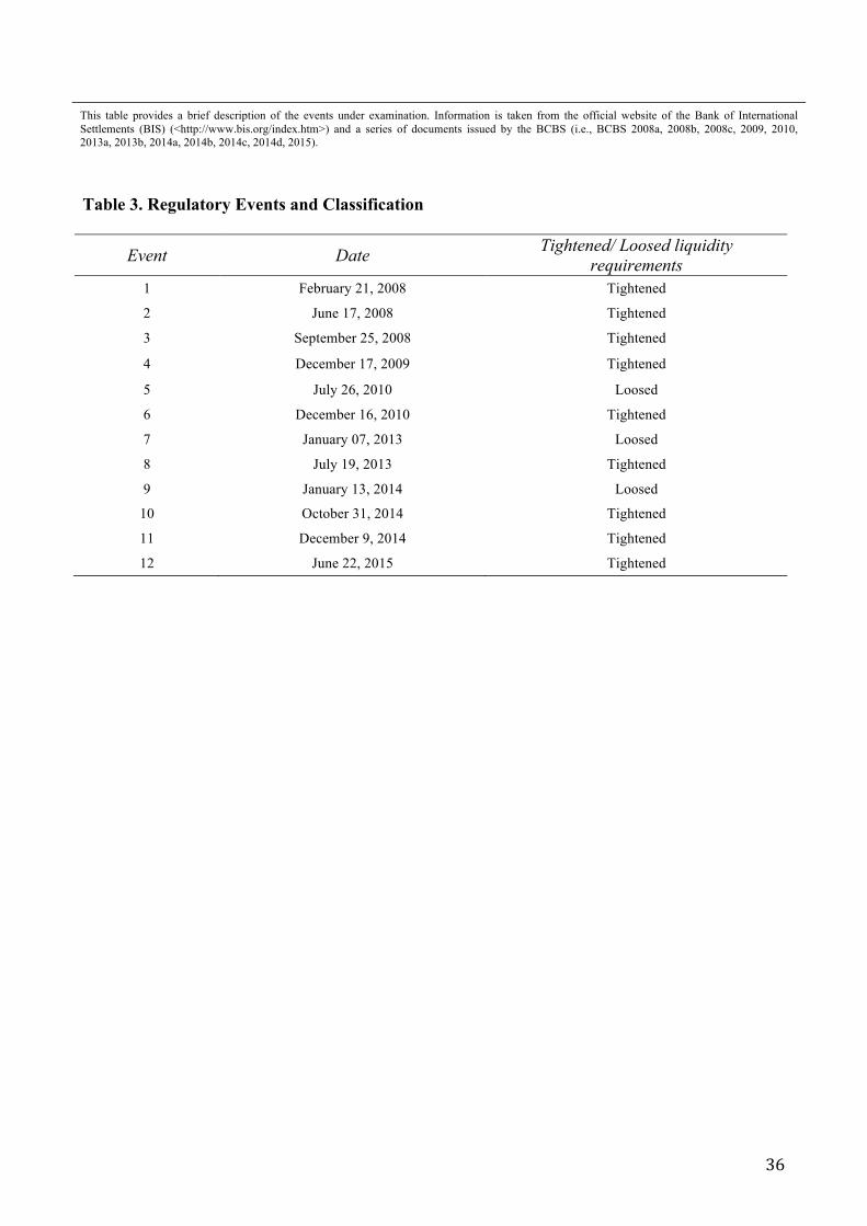
36

This table provides a brief description of the events under examination. Information is taken from the official website of the Bank of International Settlements (BIS) (<http://www.bis.org/index.htm>) and a series of documents issued by the BCBS (i.e., BCBS 2008a, 2008b, 2008c, 2009, 2010, 2013a, 2013b, 2014a, 2014b, 2014c, 2014d, 2015).

Table 3. Regulatory Events and Classification

Event Date Tightened/ Loosed liquidity requirements

1 February 21, 2008 Tightened

2 June 17, 2008 Tightened

3 September 25, 2008 Tightened

4 December 17, 2009 Tightened

5 July 26, 2010 Loosed

6 December 16, 2010 Tightened

7 January 07, 2013 Loosed

8 July 19, 2013 Tightened

9 January 13, 2014 Loosed

10 October 31, 2014 Tightened

11 December 9, 2014 Tightened

12 June 22, 2015 Tightened

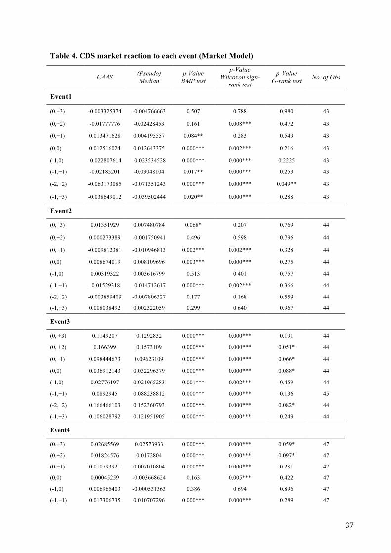
37

Table 4. CDS market reaction to each event (Market Model)

CAAS (Pseudo) Median

p-Value BMP test

p-Value Wilcoxon sign-

rank test

p-Value G-rank test No. of Obs

Event1

(0,+3) -0.003325374 -0.004766663 0.507 0.788 0.980 43

(0,+2) -0.01777776 -0.02428453 0.161 0.008*** 0.472 43

(0,+1) 0.013471628 0.004195557 0.084** 0.283 0.549 43

(0,0) 0.012516024 0.012643375 0.000*** 0.002*** 0.216 43

(-1,0) -0.022807614 -0.023534528 0.000*** 0.000*** 0.2225 43

(-1,+1) -0.02185201 -0.03048104 0.017** 0.000*** 0.253 43

(-2,+2) -0.063173085 -0.071351243 0.000*** 0.000*** 0.049** 43

(-1,+3) -0.038649012 -0.039502444 0.020** 0.000*** 0.288 43

Event2

(0,+3) 0.01351929 0.007480784 0.068* 0.207 0.769 44

(0,+2) 0.000273389 -0.001750941 0.496 0.598 0.796 44

(0,+1) -0.009812381 -0.010946813 0.002*** 0.002*** 0.328 44

(0,0) 0.008674019 0.008109696 0.003*** 0.000*** 0.275 44

(-1,0) 0.00319322 0.003616799 0.513 0.401 0.757 44

(-1,+1) -0.01529318 -0.014712617 0.000*** 0.002*** 0.366 44

(-2,+2) -0.003859409 -0.007806327 0.177 0.168 0.559 44

(-1,+3) 0.008038492 0.002322059 0.299 0.640 0.967 44

Event3

(0, +3) 0.1149207 0.1292832 0.000*** 0.000*** 0.191 44

(0, +2) 0.166399 0.1573109 0.000*** 0.000*** 0.051* 44

(0,+1) 0.098444673 0.09623109 0.000*** 0.000*** 0.066* 44

(0,0) 0.036912143 0.032296379 0.000*** 0.000*** 0.088* 44

(-1,0) 0.02776197 0.021965283 0.001*** 0.002*** 0.459 44

(-1,+1) 0.0892945 0.088238812 0.000*** 0.000*** 0.136 45

(-2,+2) 0.166466103 0.152360793 0.000*** 0.000*** 0.082* 44

(-1,+3) 0.106028792 0.121951905 0.000*** 0.000*** 0.249 44

Event4

(0,+3) 0.02685569 0.02573933 0.000*** 0.000*** 0.059* 47

(0,+2) 0.01824576 0.0172804 0.000*** 0.000*** 0.097* 47

(0,+1) 0.010793921 0.007010804 0.000*** 0.000*** 0.281 47

(0,0) 0.00045259 -0.003668624 0.163 0.005*** 0.422 47

(-1,0) 0.006965403 -0.000531363 0.386 0.694 0.896 47

(-1,+1) 0.017306735 0.010707296 0.000*** 0.000*** 0.289 47

38

(-2,+2) 0.019630976 0.015684165 0.000*** 0.000*** 0.183 47

(-1,+3) 0.033368508 0.029986101 0.000*** 0.000*** 0.048** 47

Event5

(0,+3) -0.06734231 -0.07093104 0.000*** 0.000*** 0.045** 47

(0,+2) -0.06951166 -0.07259905 0.000*** 0.000*** 0.044** 47

(0,+1) -0.072536787 -0.073658403 0.000*** 0.000*** 0.037** 47

(0,0) -0.013711473 -0.014458642 0.000*** 0.000*** 0.222 47

(-1,0) -0.022467941 -0.023591625 0.000*** 0.000*** 0.065* 47

(-1,+1) -0.081293256 -0.082843935 0.000*** 0.000*** 0.023** 47

(-2,+2) -0.087095481 -0.090402043 0.000** 0.000*** 0.025** 47

(-1,+3) -0.076098782 -0.079998779 0.000*** 0.000*** 0.033** 47

Event6

(0, +3) 0.0525239 0.05056578 0.000*** 0.000*** 0.052* 47

(0, +2) 0.03874857 0.03599156 0.000*** 0.000*** 0.094* 47

(0,+1) 0.029007961 0.023385866 0.000*** 0.000*** 0.189 47

(0,0) 0.011872354 0.005877116 0.014** 0.008*** 0.626 47

(-1,0) -0.000467986 -0.005671869 0.436 0.119 0.653 47

(-1,+1) 0.016667621 0.010659103 0.006*** 0.006*** 0.537 47

(-2,+2) 0.015965334 0.013717786 0.018** 0.013** 0.497 47

(-1,+3) 0.040183562 0.038288544 0.000*** 0.000*** 0.091* 47

Event7

(0, +3) -0.02348527 -0.01499504 0.023** 0.037** 0.516 47

(0, +2) -0.02247834 -0.01653599 0.003*** 0.005*** 0.360 47

(0,+1) -0.0225372 -0.019054332 0.000*** 0.001*** 0.293 47

(0,0) -0.015523083 -0.01206886 0.000*** 0.001*** 0.265 47

(-1,0) -0.018017048 -0.016061784 0.000*** 0.000*** 0.163 47

(-1,+1) -0.025031165 -0.022965042 0.000*** 0.000*** 0.182 47

(-2,+2) -0.022916956 -0.015253382 0.030** 0.050* 0.516 47

(-1,+3) -0.025979236 -0.019197108 0.003*** 0.006*** 0.374 47

Event8

(0,+3) -0.01875879 -0.01879081 0.000*** 0.000*** 0.210 49

(0,+2) -0.01080068 -0.01027948 0.006*** 0.002*** 0.360 49

(0,+1) -0.005065828 -0.004437887 0.155 0.099* 0.730 49

(0,0) -0.001276596 -0.001971206 0.331 0.119 0.740 49

(-1,0) -0.002910442 -0.002001618 0.333 0.424 0.917 49

(-1,+1) -0.006699675 -0.005130719 0.180 0.198 0.808 49

(-2,+2) -0.008075789 -0.005927135 0.105 0.121 0.734 49

(-1,+3) -0.020392635 -0.019586878 0.001*** 0.000*** 0.308 49

Event9

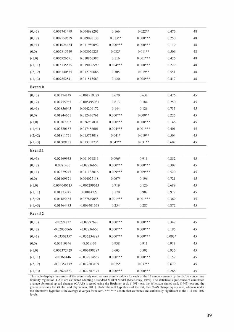
39

(0,+3) 0.003741499 0.004988203 0.166 0.022** 0.476 48

(0,+2) 0.007559659 0.009020138 0.013** 0.000*** 0.250 48

(0,+1) 0.011024484 0.011950092 0.000*** 0.000*** 0.119 48

(0,0) 0.002815549 0.003029223 0.082* 0.011** 0.506 48

(-1,0) 0.006926591 0.010856387 0.116 0.001*** 0.426 48

(-1,+1) 0.015135525 0.019006599 0.004*** 0.000*** 0.229 48

(-2,+2) 0.006140535 0.012760666 0.305 0.019** 0.551 48

(-1,+3) 0.007852541 0.011515583 0.120 0.004*** 0.417 48

Event10

(0,+3) 0.00374149 -0.001919329 0.670 0.638 0.476 45

(0,+2) 0.00755965 -0.005495031 0.813 0.184 0.250 45

(0,+1) 0.00856945 0.004209172 0.144 0.126 0.735 45

(0,0) 0.01844661 0.012476761 0.000*** 0.000** 0.225 45

(-1,0) 0.03307902 0.026937831 0.000*** 0.000*** 0.146 45

(-1,+1) 0.02320187 0.017486601 0.004*** 0.001*** 0.401 45

(-2,+2) 0.01811771 0.015753018 0.041* 0.019** 0.504 45

(-1,+3) 0.01609135 0.013302735 0.047** 0.031** 0.602 45

Event11

(0,+3) 0.02469933 0.001079815 0.096* 0.911 0.852 45

(0,+2) 0.0381436 -0.02836666 0.000*** 0.000*** 0.307 45

(0,+1) 0.02279245 0.011135016 0.009*** 0.009*** 0.520 45

(0,0) 0.01409571 0.004027118 0.067* 0.196 0.721 45

(-1,0) 0.004040715 -0.007299633 0.719 0.120 0.689 45

(-1,+1) 0.01273745 0.00014722 0.170 0.982 0.977 45

(-2,+2) 0.04185485 0.027849055 0.001*** 0.001*** 0.369 45

(-1,+3) 0.01464433 -0.009401658 0.254 0.287 0.872 45

Event12

(0,+3) -0.0224277 -0.02297626 0.000*** 0.000*** 0.342 45

(0,+2) -0.02836066 -0.02836666 0.000*** 0.000*** 0.195 45

(0,+1) -0.03302357 -0.035234885 0.000*** 0.000*** 0.093* 45

(0,0) 0.00719346 -8.06E-05 0.938 0.911 0.913 45

(-1,0) 0.003372429 -0.003498387 0.603 0.502 0.936 45

(-1,+1) -0.0368446 -0.039814635 0.000*** 0.000*** 0.152 45

(-2,+2) -0.01354739 -0.012603109 0.075* 0.037** 0.679 45

(-1,+3) -0.02624873 -0.027387375 0.000*** 0.000*** 0.268 45 This table displays the results of the event study over various event windows for each of the 12 announcements by the BCBS concerning liquidity regulation. CASs are estimated adopting a standard Market Model (MacKinlay, 1997). The statistical significance of cumulated average abnormal spread changes (CAAS) is tested using the Boehmer et al. (1991) test, the Wilcoxon signed-rank (1945) test and the generalized rank test (Kolari and Phynnonen, 2011). Under the null hypothesis of the test, the CAAS change equals zero, whereas under the alternative hypothesis the average diverges from zero. ***,**,* denote that estimates are statistically significant at the 1, 5 and 10% levels.

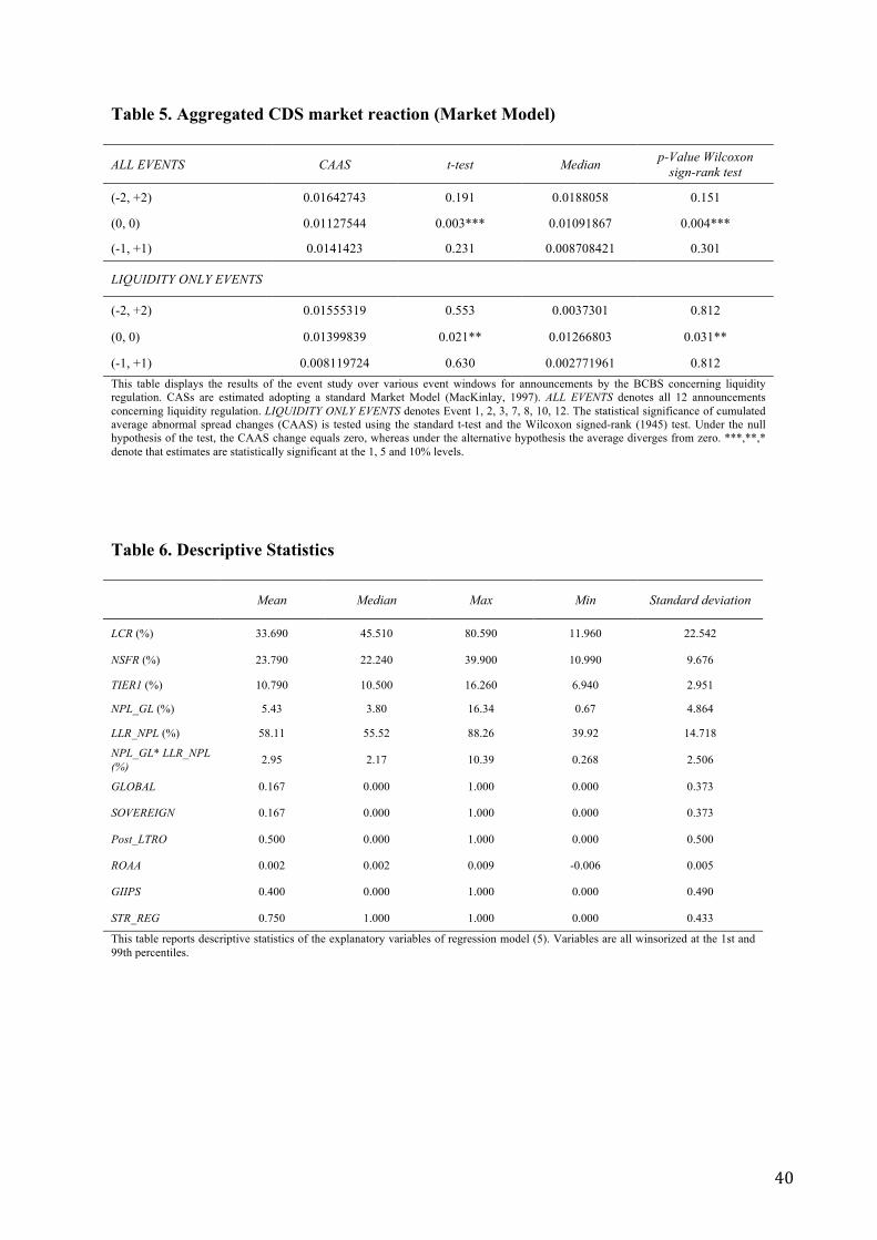
40

Table 5. Aggregated CDS market reaction (Market Model)

ALL EVENTS CAAS t-test Median p-Value Wilcoxon sign-rank test

(-2, +2) 0.01642743 0.191 0.0188058 0.151

(0, 0) 0.01127544 0.003*** 0.01091867 0.004***

(-1, +1) 0.0141423 0.231 0.008708421 0.301

LIQUIDITY ONLY EVENTS

(-2, +2) 0.01555319 0.553 0.0037301 0.812

(0, 0) 0.01399839 0.021** 0.01266803 0.031**

(-1, +1) 0.008119724 0.630 0.002771961 0.812 This table displays the results of the event study over various event windows for announcements by the BCBS concerning liquidity regulation. CASs are estimated adopting a standard Market Model (MacKinlay, 1997). ALL EVENTS denotes all 12 announcements concerning liquidity regulation. LIQUIDITY ONLY EVENTS denotes Event 1, 2, 3, 7, 8, 10, 12. The statistical significance of cumulated average abnormal spread changes (CAAS) is tested using the standard t-test and the Wilcoxon signed-rank (1945) test. Under the null hypothesis of the test, the CAAS change equals zero, whereas under the alternative hypothesis the average diverges from zero. ***,**,* denote that estimates are statistically significant at the 1, 5 and 10% levels.

Table 6. Descriptive Statistics

Mean Median Max Min Standard deviation

LCR (%) 33.690 45.510 80.590 11.960 22.542

NSFR (%) 23.790 22.240 39.900 10.990 9.676

TIER1 (%) 10.790 10.500 16.260 6.940 2.951

NPL_GL (%) 5.43 3.80 16.34 0.67 4.864

LLR_NPL (%) 58.11 55.52 88.26 39.92 14.718

NPL_GL* LLR_NPL (%) 2.95 2.17 10.39 0.268 2.506

GLOBAL 0.167 0.000 1.000 0.000 0.373

SOVEREIGN 0.167 0.000 1.000 0.000 0.373

Post_LTRO 0.500 0.000 1.000 0.000 0.500

ROAA 0.002 0.002 0.009 -0.006 0.005

GIIPS 0.400 0.000 1.000 0.000 0.490

STR_REG 0.750 1.000 1.000 0.000 0.433

This table reports descriptive statistics of the explanatory variables of regression model (5). Variables are all winsorized at the 1st and 99th percentiles.

41

Table 7. Correlation Matrix

LCR NSFR TIER1 NPL_GL LLR_NPL NPL_GL* LLR_NPL GLOBAL SOVEREIGN Post_LTRO ROAA GIIPS STR_REG

LCR 1.00

NSFR -0.115 1.00

TIER1 -0.032 -0.295 1.00

NPL_GL -0.369 -0.178 0.174 1.00

LLR_NPL -0.042 0.271 -0.333 -0.291 1.00

NPL_GL* LLR_NPL -0.380 -0.155 0.123 0.952 -0.074 1.00

GLOBAL 0.116 0.094 -0.399 -0.273 0.169 -0.259 1.00

SOVEREIGN 0.093 0.084 -0.091 -0.067 -0.080 -0.085 -0.204 1.00

Post_LTRO -0.296 -0.227 0.689 0.480 -0.241 0.472 -0.449 -0.451 1.00

ROAA 0.012 0.154 -0.241 -0.439 0.215 -0.428 0.194 -0.094 -0.355 1.00

GIIPS -0.410 0.277 -0.254 0.418 0.278 0.455 0.016 0.012 -0.042 0.042 1.00

STR_REG 0.068 0.032 -0.206 -0.152 0.134 -0.137 0.261 -0.259 -0.190 0.201 0.012 1.00

This table reports correlation coefficient of the explanatory variables of the regression model (5). Variables are all winsorized at the 1st and 99th percentiles.

42

Table 8. Bank CDS market reaction to liquidity regulation announcements (Market Model)– All events

ALL EVENTS (1) (2) (3) (4)

CAS(0; 0) CAS(0; +1) CAS(-1; +1) CAS(-2; +2)

LCR -5.8344e-05 -7.3223e-05 -3.1661e-04*** -1.8783e-04*

3.9726e-05 8.8086e-05 9.9745e-05 1.0670e-04

NSFR -2.7839e-04*** -5.4141e-04*** -4.3054e-04** -3.0019e-04

9.5634e-05 1.8599e-04 1.8708e-04 2.7346e-04

TIER1 -1.7175e-03*** -4.2208e-03*** -3.2354e-03*** -3.5646e-03***

4.7927e-04 6.6425e-04 9.4563e-04 8.7707e-04

NPL_GL 3.8032e-03** 6.8289e-03** 5.9791e-03* 6.1821e-03

1.6800e-03 3.4065e-03 3.4772e-03 4.0770e-03

LLR_NPL 5.8128e-05 2.5226e-04 1.0005e-04 1.8216e-04

1.7217e-04 3.1216e-04 3.6172e-04 4.7568e-04

NPL_GL*LLR_NPL -5.2339e-05* -1.1085e-04** -1.0409e-04* -9.1971e-05

2.6647e-05 5.5539e-05 5.8453e-05 7.4733e-05

GLOBAL 7.6994e-03 5.5345e-02*** 7.1161e-02*** 1.2854e-01***

6.7643e-03 1.3221e-02 1.2431e-02 1.6125e-02

SOVEREIGN 3.8859e-05 5.9343e-03 9.5106e-03 3.5058e-02***

4.4782e-03 6.6766e-03 6.7484e-03 1.2030e-02

Post_LTRO 1.2118e-03 2.7828e-02*** 3.8489e-02*** 7.6285e-02***

4.6057e-03 7.3483e-03 8.6646e-03 1.1513e-02

ROAA 5.1910e-01 1.8410e+00*** 1.4579e+00* 3.0963e+00**

4.4269e-01 6.0390e-01 7.6708e-01 1.2581e+00

GIIPS -3.4802e-03 -1.2148e-02*** -1.0550e-02** -2.0925e-02**

2.8578e-03 4.6268e-03 4.6533e-03 9.6593e-03

STR_REG 1.8021e-02*** 3.2045e-02*** 3.0997e-02*** 4.1910e-02***

4.5683e-03 7.5187e-03 8.4883e-03 1.0703e-02

Constant 9.7611e-03 -1.3888e-03 -8.1297e-03 -5.4984e-02

1.7059e-02 2.5845e-02 2.8467e-02 3.7186e-02

Observations 501 501 501 501

Adjusted R-squared 0.121 0.199 0.194 0.264 This table reports the results from the regression analysis for 12 events concerning liquidity regulation. The estimation is an OLS regression with clustered standard errors at the country level. CASs are estimated adopting a standard Market Model (MacKinlay, 1997). TIER1 is the ratio between primary regulatory capital and risk weighted assets. LCR is the ratio of liquid assets to deposits and short-term funding; NSFR is the ratio of equity and long-term funding in total assets; NPL_GL is the ratio between impaired loans and gross loans; LLR_NPL is the ratio between loan loss reserves and non-performing loans; GLOBAL is a dummy variable for the global crisis period (15/09/2008-01/05/2010); SOVEREIGN is a dummy variable for the sovereign debt crisis period (02/05/2010-21/12/2011); Post_LTRO is a dummy variable for the period following the two LTROs by the ECB (after 22/12/2011); ROAA is the return on average assets; GIIPS is a dummy variable for banks located in Greece, Ireland, Italy, Portugal and Spain; STR_REG is a dummy variable indicating the events expected to increase the regulation on liquidity. Regressors are all winsorized at the 1st and 99th percentiles. Standard errors clustered at the country level are reported in parenthesis. ***, **, and ∗ indicate statistical significance at 1%, 5%, and 10%.

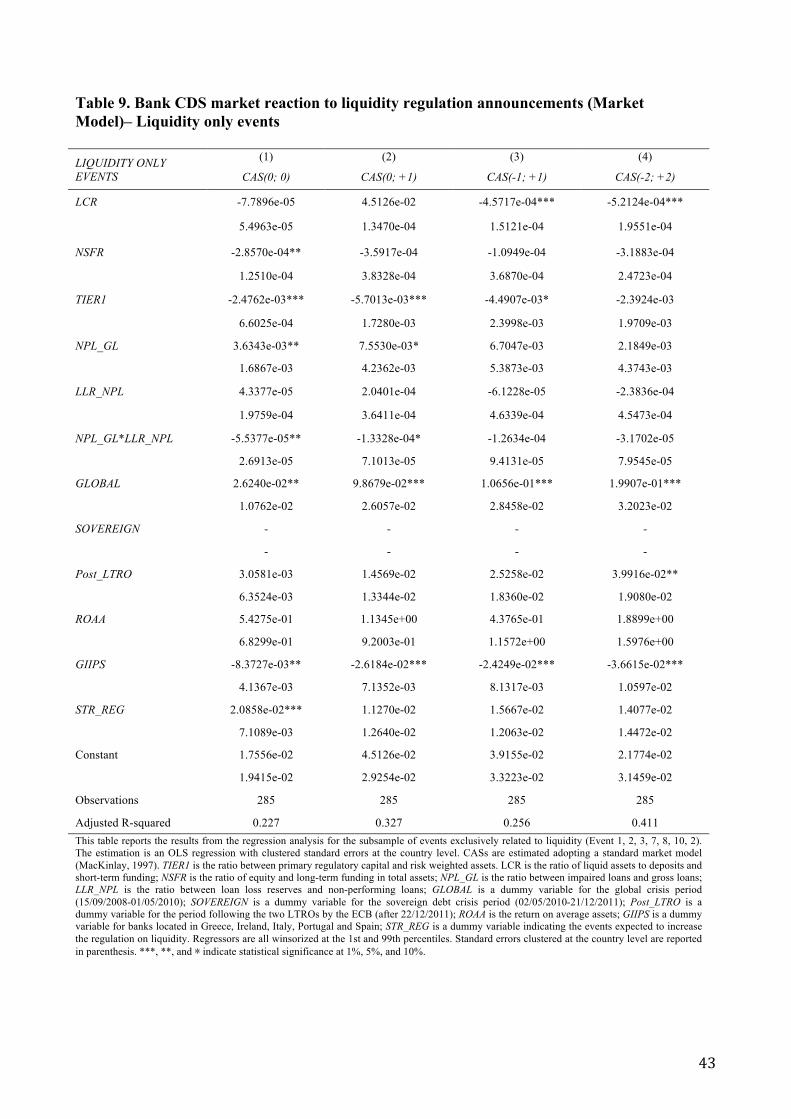
43

Table 9. Bank CDS market reaction to liquidity regulation announcements (Market Model)– Liquidity only events LIQUIDITY ONLY EVENTS

(1) (2) (3) (4)

CAS(0; 0) CAS(0; +1) CAS(-1; +1) CAS(-2; +2)

LCR -7.7896e-05 4.5126e-02 -4.5717e-04*** -5.2124e-04***

5.4963e-05 1.3470e-04 1.5121e-04 1.9551e-04

NSFR -2.8570e-04** -3.5917e-04 -1.0949e-04 -3.1883e-04

1.2510e-04 3.8328e-04 3.6870e-04 2.4723e-04

TIER1 -2.4762e-03*** -5.7013e-03*** -4.4907e-03* -2.3924e-03

6.6025e-04 1.7280e-03 2.3998e-03 1.9709e-03

NPL_GL 3.6343e-03** 7.5530e-03* 6.7047e-03 2.1849e-03

1.6867e-03 4.2362e-03 5.3873e-03 4.3743e-03

LLR_NPL 4.3377e-05 2.0401e-04 -6.1228e-05 -2.3836e-04

1.9759e-04 3.6411e-04 4.6339e-04 4.5473e-04

NPL_GL*LLR_NPL -5.5377e-05** -1.3328e-04* -1.2634e-04 -3.1702e-05

2.6913e-05 7.1013e-05 9.4131e-05 7.9545e-05

GLOBAL 2.6240e-02** 9.8679e-02*** 1.0656e-01*** 1.9907e-01***

1.0762e-02 2.6057e-02 2.8458e-02 3.2023e-02

SOVEREIGN - - - -

- - - -

Post_LTRO 3.0581e-03 1.4569e-02 2.5258e-02 3.9916e-02**

6.3524e-03 1.3344e-02 1.8360e-02 1.9080e-02

ROAA 5.4275e-01 1.1345e+00 4.3765e-01 1.8899e+00

6.8299e-01 9.2003e-01 1.1572e+00 1.5976e+00

GIIPS -8.3727e-03** -2.6184e-02*** -2.4249e-02*** -3.6615e-02***

4.1367e-03 7.1352e-03 8.1317e-03 1.0597e-02

STR_REG 2.0858e-02*** 1.1270e-02 1.5667e-02 1.4077e-02

7.1089e-03 1.2640e-02 1.2063e-02 1.4472e-02

Constant 1.7556e-02 4.5126e-02 3.9155e-02 2.1774e-02

1.9415e-02 2.9254e-02 3.3223e-02 3.1459e-02

Observations 285 285 285 285

Adjusted R-squared 0.227 0.327 0.256 0.411 This table reports the results from the regression analysis for the subsample of events exclusively related to liquidity (Event 1, 2, 3, 7, 8, 10, 2). The estimation is an OLS regression with clustered standard errors at the country level. CASs are estimated adopting a standard market model (MacKinlay, 1997). TIER1 is the ratio between primary regulatory capital and risk weighted assets. LCR is the ratio of liquid assets to deposits and short-term funding; NSFR is the ratio of equity and long-term funding in total assets; NPL_GL is the ratio between impaired loans and gross loans; LLR_NPL is the ratio between loan loss reserves and non-performing loans; GLOBAL is a dummy variable for the global crisis period (15/09/2008-01/05/2010); SOVEREIGN is a dummy variable for the sovereign debt crisis period (02/05/2010-21/12/2011); Post_LTRO is a dummy variable for the period following the two LTROs by the ECB (after 22/12/2011); ROAA is the return on average assets; GIIPS is a dummy variable for banks located in Greece, Ireland, Italy, Portugal and Spain; STR_REG is a dummy variable indicating the events expected to increase the regulation on liquidity. Regressors are all winsorized at the 1st and 99th percentiles. Standard errors clustered at the country level are reported in parenthesis. ***, **, and ∗ indicate statistical significance at 1%, 5%, and 10%.

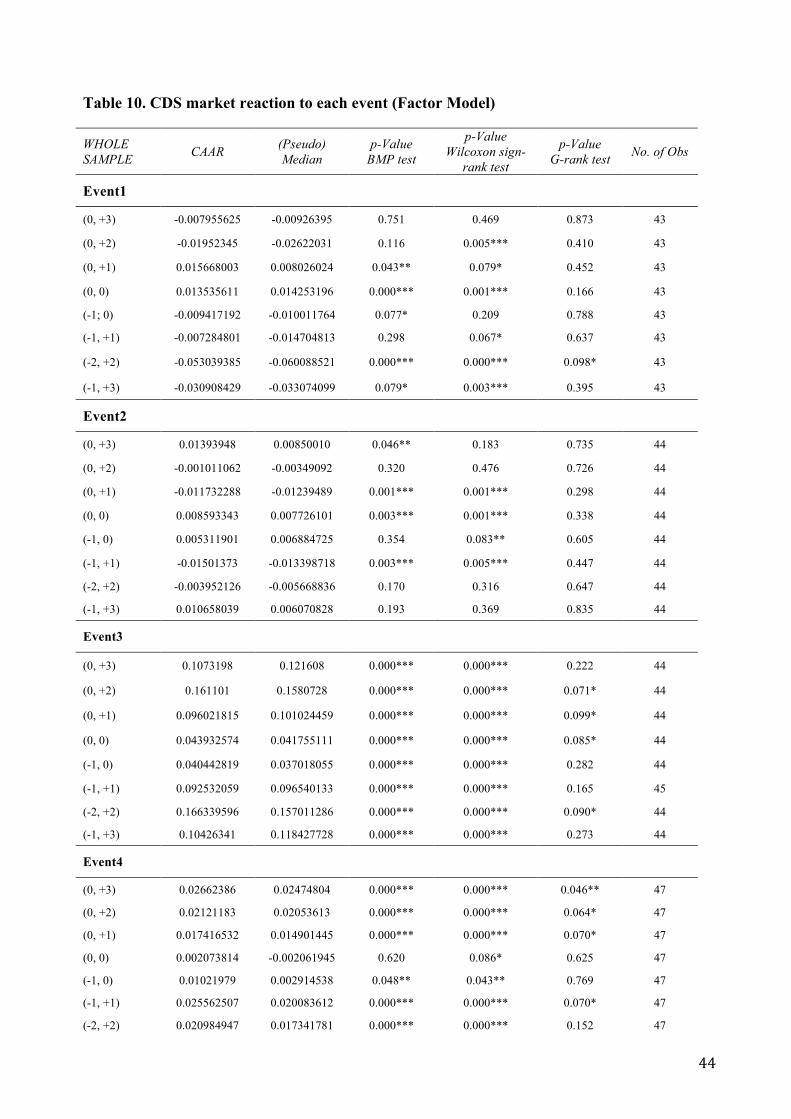
44

Table 10. CDS market reaction to each event (Factor Model)

WHOLE SAMPLE CAAR (Pseudo)

Median p-Value

BMP test

p-Value Wilcoxon sign-

rank test

p-Value G-rank test No. of Obs

Event1

(0, +3) -0.007955625 -0.00926395 0.751 0.469 0.873 43

(0, +2) -0.01952345 -0.02622031 0.116 0.005*** 0.410 43

(0, +1) 0.015668003 0.008026024 0.043** 0.079* 0.452 43

(0, 0) 0.013535611 0.014253196 0.000*** 0.001*** 0.166 43

(-1; 0) -0.009417192 -0.010011764 0.077* 0.209 0.788 43

(-1, +1) -0.007284801 -0.014704813 0.298 0.067* 0.637 43

(-2, +2) -0.053039385 -0.060088521 0.000*** 0.000*** 0.098* 43

(-1, +3) -0.030908429 -0.033074099 0.079* 0.003*** 0.395 43

Event2

(0, +3) 0.01393948 0.00850010 0.046** 0.183 0.735 44

(0, +2) -0.001011062 -0.00349092 0.320 0.476 0.726 44

(0, +1) -0.011732288 -0.01239489 0.001*** 0.001*** 0.298 44

(0, 0) 0.008593343 0.007726101 0.003*** 0.001*** 0.338 44

(-1, 0) 0.005311901 0.006884725 0.354 0.083** 0.605 44

(-1, +1) -0.01501373 -0.013398718 0.003*** 0.005*** 0.447 44

(-2, +2) -0.003952126 -0.005668836 0.170 0.316 0.647 44

(-1, +3) 0.010658039 0.006070828 0.193 0.369 0.835 44

Event3

(0, +3) 0.1073198 0.121608 0.000*** 0.000*** 0.222 44

(0, +2) 0.161101 0.1580728 0.000*** 0.000*** 0.071* 44

(0, +1) 0.096021815 0.101024459 0.000*** 0.000*** 0.099* 44

(0, 0) 0.043932574 0.041755111 0.000*** 0.000*** 0.085* 44

(-1, 0) 0.040442819 0.037018055 0.000*** 0.000*** 0.282 44

(-1, +1) 0.092532059 0.096540133 0.000*** 0.000*** 0.165 45

(-2, +2) 0.166339596 0.157011286 0.000*** 0.000*** 0.090* 44

(-1, +3) 0.10426341 0.118427728 0.000*** 0.000*** 0.273 44

Event4

(0, +3) 0.02662386 0.02474804 0.000*** 0.000*** 0.046** 47

(0, +2) 0.02121183 0.02053613 0.000*** 0.000*** 0.064* 47

(0, +1) 0.017416532 0.014901445 0.000*** 0.000*** 0.070* 47

(0, 0) 0.002073814 -0.002061945 0.620 0.086* 0.625 47

(-1, 0) 0.01021979 0.002914538 0.048** 0.043** 0.769 47

(-1, +1) 0.025562507 0.020083612 0.000*** 0.000*** 0.070* 47

(-2, +2) 0.020984947 0.017341781 0.000*** 0.000*** 0.152 47

45

(-1, +3) 0.034769839 0.030690401 0.000*** 0.000*** 0.040** 47

Event5

(0, +3) -0.06566583 -0.06894547 0.000*** 0.000*** 0.044** 47

(0, +2) -0.06687071 -0.06968607 0.000*** 0.000*** 0.045** 47

(0, +1) -0.065617434 -0.066978132 0.000*** 0.000*** 0.047** 47

(0, 0) -0.009750127 -0.010459518 0.001*** 0.001*** 0.369 47

(-1, 0) -0.011653053 -0.013817249 0.003*** 0.001*** 0.311 47

(-1, +1) -0.06752036 -0.06851872 0.000*** 0.000*** 0.041** 47

(-2, +2) -0.078730665 -0.082370396 0.000*** 0.000*** 0.038** 47

(-1, +3) -0.067568756 -0.072023028 0.000*** 0.000*** 0.046** 47

Event6

(0, +3) 0.0484992 0.0463966 0.000*** 0.000*** 0.070* 47

(0, +2) 0.03582404 0.03380778 0.000*** 0.000*** 0.113 47

(0, +1) 0.028079223 0.022992708 0.000*** 0.000*** 0.192 47

(0, 0) 0.01145703 0.00616314 0.019** 0.020** 0.639 47

(-1, 0) -0.00148841 -0.007049649 0.321 0.094* 0.595 47

(-1, +1) 0.015133783 0.009614019 0.015** 0.015** 0.597 47

(-2, +2) 0.015878462 0.013889231 0.020** 0.015** 0.536 47

(-1, +3) 0.035553759 0.03423154 0.000*** 0.000*** 0.131 47

Event7

(0, +3) -0.02252314 -0.01477398 0.028** 0.052* 0.538 47

(0, +2) -0.02193604 -0.01597063 0.006*** 0.015** 0.413 47

(0, +1) -0.021544339 -0.017827856 0.001*** 0.002*** 0.329 47

(0, 0) -0.014560635 -0.011509028 0.001*** 0.002*** 0.316 47

(-1, 0) -0.017115103 -0.014776173 0.000*** 0.000*** 0.200 47

(-1, +1) -0.024098807 -0.021952723 0.000*** 0.000*** 0.207 47

(-2, +2) -0.019466994 -0.012762144 0.087* 0.109 0.611 47

(-1, +3) -0.025077604 -0.020178145 0.004*** 0.009*** 0.387 47

Event8

(0, +3) -0.01560179 -0.01616338 0.001*** 0.000*** 0.294 49

(0, +2) -0.01278211 -0.01282794 0.001*** 0.000*** 0.271 49

(0, +1) -0.006960535 -0.006494897 0.053* 0.022** 0.539 49

(0, 0) -0.002749722 -0.003787357 0.097* 0.025** 0.478 49

(-1, 0) -0.002541881 -0.001545624 0.424 0.541 0.938 49

(-1, +1) -0.006752694 -0.004790032 0.172 0.178 0.753 49

(-2, +2) -0.008726775 -0.007044902 0.069* 0.089* 0.649 49

(-1, +3) -0.015393952 -0.014146483 0.011** 0.009*** 0.465 49

Event9

(0, +3) 0.005948914 0.006163691 0.044** 0.000*** 0.441 48

46

(0, +2) 0.01004998 0.01154118 0.002*** 0.000*** 0.228 48

(0, +1) 0.012124131 0.013065315 0.000*** 0.000*** 0.114 48

(0, 0) 0.004455991 0.004489807 0.008*** 0.001*** 0.391 48

(-1, 0) 0.009847104 0.01342367 0.028** 0.000*** 0.322 48

(-1, +1) 0.017515244 0.020965724 0.001*** 0.000*** 0.186 48

(-2, +2) 0.009515096 0.015509119 0.125 0.005*** 0.510 48

(-1, +3) 0.011340026 0.014499099 0.034** 0.000*** 0.381 48

Event10

(0, +3) 0.004241473 0.000652322 0.476 0.858 0.909 45

(0, +2) 0.001542321 -0.001794173 0.238 0.687 0.956 45

(0, +1) 0.01035577 0.006299396 0.415 0.046* 0.643 45

(0, 0) 0.02031283 0.015047519 0.012** 0.000*** 0.215 45

(-1, 0) 0.03620994 0.030347656 0.000*** 0.000*** 0.126 45

(-1, +1) 0.02625288 0.021111642 0.002*** 0.000*** 0.319 45

(-2, +2) 0.02277107 0.019363373 0.007*** 0.003*** 0.406 45

(-1, +3) 0.02013858 0.016240338 0.040** 0.010** 0.526 45

Event11

(0, +3) 0.03007008 0.007656314 0.225 0.238 0.697 45

(0, +2) 0.0405375 0.02555965 0.002*** 0.000*** 0.253 45

(0, +1) 0.02620798 0.015840057 0.002*** 0.001*** 0.396 45

(0, 0) 0.01772403 0.009282026 0.010** 0.004*** 0.497 45

(-1, 0) 0.00887868 -0.001734496 0.771 0.696 0.969 45

(-1, +1) 0.01736263 0.005297978 0.166 0.287 0.727 45

(-2, +2) 0.0436291 0.029663363 0.002*** 0.000*** 0.325 45

(-1, +3) 0.02122473 -0.003202693 0.828 0.679 0.932 45

Event12

(0, +3) -0.02115577 -0.0219584 0.000*** 0.001*** 0.373 45

(0, +2) -0.02626573 -0.02634109 0.000*** 0.000*** 0.244 45

(0, +1) -0.03108875 -0.033704378 0.000*** 0.000*** 0.066* 45

(0, 0) 0.009750231 0.001968318 0.376 0.576 0.791 45

(-1, 0) 0.004625008 -0.003185215 0.787 0.568 0.938 45

(-1, +1) -0.03621397 -0.040143514 0.000*** 0.000*** 0.151 45

(-2, +2) -0.01167597 -0.011559641 0.009*** 0.071* 0.739 45

(-1, +3) -0.02628099 -0.028814769 0.000*** 0.000*** 0.278 45 This table displays the results of the event study over various event windows for each of the 12 announcements by the BCBS concerning liquidity regulation. CASs are estimated adopting a factor model. The statistical significance of cumulated average abnormal spread changes (CAAS) is tested using the Boehmer et al. (1991) test, the Wilcoxon signed-rank (1945) test and the generalized rank test (Kolari and Phynnonen, 2011). Under the null hypothesis of the test, the CAAS change equals zero, whereas under the alternative hypothesis the average diverges from zero. ***,**,* denote that estimates are statistically significant at the 1, 5 and 10% levels.

47

Table 11. Aggregated CDS market reaction (Factor Model)

ALL EVENTS CAAS t-test Median p-Value Wilcoxon sign-rank test

(-2, +2) 0.02340762 0.172 0.01651678 0.151

(0, 0) 0.01204038 0.006*** 0.0111289 0.005***

(-1, +1) 0.01547355 0.169 0.00961706 0.203

LIQUIDITY ONLY EVENTS

(-2, +2) 0.01874049 0.503 0.00545882 0.812

(0, 0) 0.01541936 0.030** 0.01379187 0.031**

(-1, +1) 0.01108836 0.511 0.00701328 0.812 This table displays the results of the event study over various event windows for announcements by the BCBS concerning liquidity regulation. CASs are estimated adopting a factor model. ALL EVENTS denotes all 12 announcements concerning liquidity regulation. LIQUIDITY ONLY EVENTS denotes Event 1, 2, 3, 7, 8, 10, 12. The statistical significance of cumulated average abnormal spread changes (CAAS) is tested using the standard t-test and the Wilcoxon signed-rank (1945) test. Under the null hypothesis of the test, the CAAS change equals zero, whereas under the alternative hypothesis the average diverges from zero. ***,**,* denote that estimates are statistically significant at the 1, 5 and 10% levels.

48

Table 12. Bank CDS market reaction to liquidity regulation announcements (Factor Model)– All events

ALL EVENTS (1) (2) (3) (4)

CAS(0; 0) CAS(0; +1) CAS(-1; +1) CAS(-2; +2)

TIER1 -1.6617e-03*** -3.8478e-03*** -2.7992e-03** -3.2360e-03***

5.3942e-04 9.7569e-04 1.2464e-03 1.0845e-03

LCR -5.2531e-05 -8.2824e-05 -3.0696e-04*** -1.6803e-04

4.7886e-05 1.0633e-04 1.0328e-04 1.1058e-04

NSFR -2.7495e-04*** -6.0762e-04*** -3.3636e-04** -2.4559e-04

7.5077e-05 1.8258e-04 1.4198e-04 2.8182e-04

NPL_GL 4.2006e-03** 5.9133e-03* 4.8576e-03 5.3445e-03

1.6604e-03 3.1400e-03 3.3080e-03 3.8551e-03

LLR_NPL 8.9107e-05 1.0289e-04 -4.2541e-05 4.8396e-05

1.5650e-04 2.2830e-04 2.9429e-04 4.6458e-04

NPL_GL*LLR_NPL -5.6597e-05** -9.3225e-05* -8.0228e-05 -7.3830e-05

2.7766e-05 5.2859e-05 5.6216e-05 7.3855e-05

GLOBAL 1.1689e-02* 5.7070e-02 6.9034e-02*** 1.2324e-01***

6.9436e-03 1.2996e-02 1.1937e-02 1.6801e-02

SOVEREIGN 5.6891e-04 5.3546e-03 3.4524e-03 3.1054e-02**

4.8831e-03 6.8673e-03 6.8821e-03 1.2732e-02

Post_LTRO 9.3330e-04 2.3864e-02*** 2.7434e-02*** 6.8773e-02***

5.6358e-03 8.4245e-03 1.0078e-02 1.4028e-02

ROAA 5.3360e-01 1.7783e+00*** 1.4408e+00** 3.1460e+00***

3.5944e-01 5.1570e-01 7.2059e-01 1.2108e+00

GIIPS -4.4505e-03 -9.1901e-03* -9.2110e-03* -1.9064e-02*

2.8390e-03 5.1016e-03 5.0707e-03 9.9291e-03

STR_REG 1.6905e-02*** 2.9751e-02*** 2.6632e-02*** 3.7621e-02***

4.9135e-03 7.8600e-03 8.7529e-03 1.0438e-02

Constant 8.2715e-03 8.6175e-03 5.6764e-03 -4.2950e-02

1.6281e-02 2.0437e-02 2.3238e-02 3.4058e-02

Observations 501 501 501 501

Adjusted R-squared 0.122 0.197 0.185 0.243 This table reports the results from the regression analysis for 12 events concerning liquidity regulation. The estimation is an OLS regression with clustered standard errors at the country level. CASs are estimated adopting a factor model. TIER1 is the ratio between primary regulatory capital and risk weighted assets. LCR is the ratio of liquid assets to deposits and short-term funding; NSFR is the ratio of equity and long-term funding in total assets; NPL_GL is the ratio between impaired loans and gross loans; LLR_NPL is the ratio between loan loss reserves and non-performing loans; GLOBAL is a dummy variable for the global crisis period (15/09/2008-01/05/2010); SOVEREIGN is a dummy variable for the sovereign debt crisis period (02/05/2010-21/12/2011); Post_LTRO is a dummy variable for the period following the two LTROs by the ECB (after 22/12/2011); ROAA is the return on average assets; GIIPS is a dummy variable for banks located in Greece, Ireland, Italy, Portugal and Spain; STR_REG is a dummy variable indicating the events expected to increase the regulation on liquidity. Regressors are all winsorized at the 1st and 99th percentiles. Standard errors clustered at the country level are reported in parenthesis. ***, **, and ∗ indicate statistical significance at 1%, 5%, and 10%.

49

Table 13. Table 10. Bank CDS market reaction to liquidity regulation announcements (Factor Model)– Liquidity only events

LIQUIDITY ONLY EVENTS

(1) (2) (3) (4)

CAS(0; 0) CAS(0; +1) CAS(-1; +1) CAS(-2; +2)

TIER1 -2.2003e-03*** -5.2555e-03** -3.8792e-03 -1.5669e-03

7.4532e-04 2.0593e-03 2.7792e-03 2.1927e-03

LCR -7.5402e-05 -1.6685e-04 -4.5442e-04*** -5.1185e-04**

6.9087e-05 1.6140e-04 1.7119e-04 2.1244e-04

NSFR -2.7367e-04** -5.5443e-04 -9.5467e-05 -2.2776e-04

1.1787e-04 3.4747e-04 2.8819e-04 2.1049e-04

NPL_GL 4.1083e-03** 6.2177e-03 4.9977e-03 1.4008e-03

1.8480e-03 4.0260e-03 5.2884e-03 4.3197e-03

LLR_NPL 5.6852e-05 -4.0488e-05 -3.0424e-04 -4.0828e-04

1.8304e-04 2.8800e-04 4.2265e-04 4.7407e-04

NPL_GL*LLR_NPL -6.1209e-05** -1.1109e-04 -9.5739e-05 -1.0163e-05

3.0501e-05 6.8744e-05 9.3088e-05 8.1087e-05

GLOBAL 3.3103e-02*** 9.6262e-02*** 1.0228e-01*** 1.9298e-01***

1.1644e-02 2.5473e-02 2.7989e-02 3.2618e-02

SOVEREIGN - - - -

- - - -

Post_LTRO 3.5567e-04 1.0479e-02 1.2635e-02 2.8712e-02

7.4837e-03 1.5353e-02 2.0296e-02 2.0619e-02

ROAA 3.8393e-01 1.1834e+00 2.3576e-01 1.8674e+00

6.3190e-01 8.7675e-01 1.1508e+00 1.5598e+00

GIIPS -8.5116e-03** -1.8718e-02*** 1.9219e-02*** -3.6093e-02***

3.8590e-03 6.2434e-03 7.3142e-03 1.0834e-02

STR_REG 2.1003e-02*** 1.0311e-02 1.5471e-02 1.2482e-02

7.7691e-03 1.3353e-02 1.2811e-02 1.4912e-02

Constant 1.4945e-02 6.0337e-02** 5.6381e-02 2.9618e-02

1.8658e-02 2.4036e-02 2.9508e-02 3.1303e-02

Observations 285 285 285 285

Adjusted R-squared 0.256 0.306 0.242 0.391 This table reports the results from the regression analysis for 12 events concerning liquidity regulation. The estimation is an OLS regression with clustered standard errors at the country level. CASs are estimated adopting a factor model. TIER1 is the ratio between primary regulatory capital and risk weighted assets. LCR is the ratio of liquid assets to deposits and short-term funding; NSFR is the ratio of equity and long-term funding in total assets; NPL_GL is the ratio between impaired loans and gross loans; LLR_NPL is the ratio between loan loss reserves and non-performing loans; GLOBAL is a dummy variable for the global crisis period (15/09/2008-01/05/2010); SOVEREIGN is a dummy variable for the sovereign debt crisis period (02/05/2010-21/12/2011); Post_LTRO is a dummy variable for the period following the two LTROs by the ECB (after 22/12/2011); ROAA is the return on average assets; GIIPS is a dummy variable for banks located in Greece, Ireland, Italy, Portugal and Spain; STR_REG is a dummy variable indicating the events expected to increase the regulation on liquidity. Regressors are all winsorized at the 1st and 99th percentiles. Standard errors clustered at the country level are reported in parenthesis. ***, **, and ∗ indicate statistical significance at 1%, 5%, and 10%.