the impacts of unscheduled lock outages
TRANSCRIPT

The Impacts of Unscheduled Lock Outages
Submitted to
Prepared for:
The National Waterways Foundation andThe U.S. Maritime Administration
Center for Transportation ResearchThe University of Tennessee
Vanderbilt Engineering Center for Transportation and Operational Resiliency Vanderbilt University
October 2017
This study was developed through a cooperative agreement between the U.S. Department of Transportation (DOT), Maritime Administration and the National
Waterways Foundation [DTMA‐91‐H1‐400009]. Opinions or points of view expressed in this document are those of the authors and do not necessarily reflect the official position
of, or a position that is endorsed by, the U.S. Government, DOT, or any sub‐agency thereof. Likewise, references to non‐Federal entities and to various methods of
infrastructure funding or financing in this document are included for illustrative purposes only and do not imply U.S. Government, DOT, or subagency endorsement of or
preference for such entities and funding methods.
The authors wish to acknowledge and thank a variety of entities that contributed to this research effort, including the Appalachian Regional Commission, the Association of
American Railroads, the U.S. Army Corps of Engineers, The Federal Railroad Administration, and the U.S. Surface Transportation Board. The authors, alone, are
responsible for any errors.
Cover Photograph courtesy of Andrew M. Turner Clarion, Pennsylvania

The Impacts of Unscheduled Lock Outages
Submitted to
The National Waterways Foundation and The U.S. Maritime Administration
by
Center for Transportation Research The University of Tennessee
Vanderbilt Engineering Center for Transportation and Operational Resiliency
Vanderbilt University
October 2017

Report Contents Executive Summary .............................................................. i. E.1 Project Context ................................................................................................ i. E.2 Lock and Dam Projects Selected for Detailed Analysis ................................. ii. E.3 Direct Shipper Supply Chain Burdens from an Unplanned Closure ............. iii. E.4 Geographic Distribution of Direct and Regional Impacts ............................. iv. E.5 Summary and Findings .................................................................................. ix.
1. Research Purpose, Context, and Approach ......................... 1. 1.1.Project Overview and Approach ...................................................................... 1. 1.2.Report Structure ............................................................................................... 2.
2. Study Methodology and Findings ........................................ 3. 2.1.Lock Selection ................................................................................................. 3. 2.2.Shipper Supply-Chain Cost Burden (SSCCB) Analysis .................................. 5. 2.3.Regional Economic Development (RED) Impact Analysis ........................... 15. 2.4.Railroad Capacity and Its Impacts on Shipper Costs ..................................... 20.
3. Screening Tool Development ............................................ 29. 3.1.Freight Data and Data Access ........................................................................ 29. 3.2.Elements and Analytics – Lock Characteristics............................................. 32. 3.3.Elements and Analytics – Lock Performance ................................................ 33. 3.4.Elements and Analytics – Network Role ....................................................... 33.
4. Estimating Closure Related Supply-Chain Cost Burdens .... 36. 4.1.Lock Selection, Traffic Samples, and Data Preparation ................................ 36. 4.2.Closure Scenarios, Shipper Alternatives and Traffic Diversions .................. 37. 4.3.Estimating Transportation Costs for Each Alternative .................................. 39. 4.4.Estimating the Shipper Supply-Chain Cost Burden....................................... 43.
5. Estimating Regional Economic Development Impacts ..... 45. 5.1.The Difference between Benefits and Impacts .............................................. 45. 5.2.The General Structure of Regional Models ................................................... 45. 5.3.Estimating Basic Economic Impact Benchmarks .......................................... 46.
6. Methodology: Final Thoughts and Recommendations ..... 51.

APPENDIX ONE – The Corridor Concentration Metric APPENDIX TWO – Lock Screening Tool Results APPENDIX THREE – Commodity-Specific Lock Traffic
List of Tables E.1 Estimated Direct Unplanned Closure Costs .......................................................... iii. E.2 Estimated Regional Impacts ................................................................................. ix.
2.1. Screening Tool Results Summary....................................................................... 4. 2.2. Closure-Related Supply Chain Cost Burden, Markland Locks & Dam ............. 9. 2.3. Closure-Related Supply Chain Cost Burden, Calcasieu Lock ............................ 9. 2.4. Closure-Related Supply Chain Cost Burden, LaGrange Lock & Dam .............. 9. 2.5. Closure-Related Supply Chain Cost Burden, Lock & Dam 25 ......................... 9. 2.6. The Economic Impacts Attributable to Markland Locks & Dam ..................... 16. 2.7. The Economic Impacts Attributable to Calcasieu Lock ................................... 17. 2.8. The Economic Impacts Attributable to LaGrange Lock & Dam ...................... 18. 2.9. The Economic Impacts Attributable to Lock & Dam 25 .................................. 19. 2.10. Summary of Railroad Traffic ............................................................................ 25. 2.11. Illustrative Rail System Impacts, LaGrange Outage ........................................ 26. 2.12. Iowa’s Water-Served Grain Terminals ............................................................. 27. 2.13. LPMS Statistics: LaGrange and L&D 25 ......................................................... 28.
3.1. Sample Annual LPMS Data ............................................................................ 30. 3.2. Sample Monthly LPMS Data .......................................................................... 30. 3.3. Base WCSC Data Record Contents ................................................................. 31.
4.1. Motor Carrier Costs ......................................................................................... 42. 4.2. Sample of Calculated Averted Supply-Chain Costs ........................................ 44.
5.1. Study-Derived Economic Impact Multipliers ................................................. 49. 5.2. RIMS II Economic Impact Multipliers (Households) ......................................50.

List of Figures E.1 Study Projects and Summary Characteristics ........................................................ ii. E.2 Markets Dependent on Markland Locks & Dam ................................................. iv. E.3 Markets Dependent on Calcasieu Lock .................................................................. v. E.4 Markets Dependent on LaGrange Lock & Dam................................................... vi. E.5 Markets Dependent on Lock & Dam 25................................................................. v. E.6 Distribution of Chemical Shipments Transiting Markland Locks & Dam ........... vi. E.7 Distribution of Coal Shipments Transiting Markland Locks & Dam .................. vi.
2.1. Locks Selected for Detailed Analysis .................................................................... 5. 2.2. Corridor Concentration Metrics ............................................................................. 7. 2.3. Markets Dependent on Markland Locks & Dam ................................................. 10. 2.4. 2014 Distribution of Chemical Shipments Transiting Markland ......................... 11. 2.5. 2014 Distribution of Coal Shipments Transiting Markland Locks & Dam ......... 11. 2.6. Markets Dependent on Calcasieu Lock ............................................................... 12. 2.7. Markets Dependent on LaGrange Lock & Dam .................................................. 13. 2.8. Markets Dependent on Lock & Dam 25 .............................................................. 14. 2.9. The Regional Employment Effects of Markland Locks & Dam ......................... 16. 2.10. The Regional Employment Impacts Attributable to Calcasieu Lock .................. 17. 2.11. The Regional Employment Impacts of LaGrange Lock & Dam ......................... 18. 2.12. The Regional Employment Impacts of Lock & Dam 25 .................................... .19. 2.13. Corridors Served by Markland and Calcasieu ..................................................... 22. 2.14. Corridors Served by LaGrange and L&D 25 ....................................................... 23. 2.15. Core Regional Rail Network ............................................................................... 24.
3.1. Above and Below Project Pool Traffic ................................................................ 35.
4.1. Shipper Responses to Unplanned Lock Closures ................................................ 38. 4.2. Barge Costing Model ........................................................................................... 40.
5.1. Representative Regional Economic Impact Construct ........................................ 46. 5.2. 2014 Study Region Geography ............................................................................ 48.
6.1 Further Communication of Study Findings ............................................................ 52.

PAGE INTENTIONALLY LEFT BLANK

i.
Executive Summary
The summarized work is the result of a study commissioned by the National Waterways Foundation and the U.S. Department of
Transportation’s Maritime Administration (MARAD). The goal of this study is to highlight the economic benefits associated with reliable
inland navigation. E.1 PROJECT CONTEXT
America’s inland waterway system was essential to the nation’s early colonial prosperity and it has been vital to U.S. commerce ever since. As navigation more fully developed in the 20th century, the waterway network became a perennial contributor to the nation’s economic success. Today, America’s waterways quietly provide an irreplaceable transportation resource that is key to the nation’s global success in the 21st century.
Unfortunately, toward the end of the 20th century, this fundamental part of U.S. transportation infrastructure became more visible, but for all the wrong reasons. Many of the nearly 200 infrastructure projects were reaching their design life of 50 years and choke points were adversely affecting more and more commercial users. The upper Mississippi’s Locks & Dam 26 and the Ohio River’s Locks & Dam 52 are examples.
Today, most navigation projects are more than 75 years old and have suffered from a persistent lack of reinvestment and environmental stresses associated with extreme weather events that magnify the system’s vulnerability.
It is within this context that the National Waterways Foundation and MARAD commissioned this study to explore the expected impacts of an extended unscheduled outage at a number of important Lock and Dam projects.
E.2 LOCK AND DAM PROJECTS SELECTED FOR DETAILED ANALYSIS
In order to assess the impact of lock availability and outages, the study team developed and used a methodology to identify a small subset of locks for closer analysis. The initial screening approach included a carefully reconciled cross-section of data describing the characteristics and performance of roughly 170 navigation locks located throughout the nation’s interior navigation system. The study team prepared and presented this information to the study’s sponsors who then selected four locks for further study based on their characteristics and

ii.
performance metrics. The map below indicates the locks selected and includes several of the key characteristics of the lock reliant traffic.
Of particular note were new metrics to assess a lock’s importance to the overall network. One such metric, noted on the map below for each project, describes the average number of locks on the system that an individual loaded barge traversing the subject lock passes through during a single movement (represented as System Lockages/Project Lockage). An additional measure shows the traffic in the pools above and below the lock that originates or terminate in the pool but does not transit the lock. While this study did not investigate the particular modalities of an unscheduled outage, it is possible that the outage could be accompanied by impacts on the pool traffic as well.
Figure E.1 – Study Projects and Summary Characteristics
E.3 DIRECT SHIPPER SUPPLY CHAIN COST BURDENS FROM AN UNSCHEDULED CLOSURE
Estimating the direct efficiency losses associated with an unplanned lock closure provided the core information on which further analysis is built. These cost estimates were derived through methods that adhere to the same Principles and Guidelines that govern U.S. Army Corps of Engineers’ navigation studies.

iii.
For each lock examined, the analysis compares an estimate of each shipper’s current costs for waterway-inclusive movements to the cost of the next best available modal alternative. Three existing models were employed that allowed a comparison of the costs associated with the use of barge service against the cost to make such a movement by rail and/or truck. For each of the four locks analyzed, the model estimates predicted the Direct Shipper Supply Chain Cost Burden if barge service becomes unavailable and, at each location, these costs would be expected to exceed $1 billion per year, as described in the Table below:
Table E.1 – Estimated Direct Unplanned Closure Costs
COMMODITY MARKLAND LOCKS & DAM LAGRANGE LOCK &DAM
Total 2014
Tons Total Direct
Costs Total 2014
Tons Total Direct
Costs Coal 30,788,869 $221,987,745 443,288 $20,291,015 Petroleum Products 7,440,371 $368,253,302 5,623,494 $182,914,135 Chemicals 3,898,264 $276,416,124 4,888,770 $251,529,491 Crude Materials 14,339,508 $242,729,791 3,401,419 $208,236,345 Primary Manufactured Goods 4,896,902 $160,394,481 3,344,289 $103,524,351 Farm Products and Food 4,089,324 $38,460,711 11,460,988 $932,684,606 Equipment 55,525 $1,818,681 5,632 $477,986 TOTAL 65,508,763 1,310,060,835 29,167,880 1,699,657,928
COMMODITY CALCASIEU LOCK L&D 25
Total 2014
Tons Total Direct
Costs Total 2014
Tons Total Direct
Costs Coal 245,836 $6,629,552 660,624 $25,696,959 Petroleum Products 24,988,887 $542,287,348 320,411 $15,103,646 Chemicals 9,078,337 $230,953,087 4,171,737 $248,899,601 Crude Materials 3,937,379 $179,789,257 3,082,613 $208,863,996 Primary Manufactured Goods 2,744,157 $120,009,771 1,667,149 $38,225,955 Farm Products and Food 843,753 $22,753,806 12,433,825 $1,033,977,564 Equipment 9,222 $248,693 6,602 $542,606 Scrap and Waste 626,896 $16,905,741 TOTAL 42,474,467 1,119,577,255 22,342,961 1,571,310,327
E.4 GEOGRAPHIC DISTRIBUTION OF THE DIRECT AND REGIONAL IMPACTS Using the information about the origins and destinations of the traffic relying on each lock, it was also possible to describe the system-wide nature of the impact which each individual lock’s closure is expected to have as illustrated on the four network maps below.
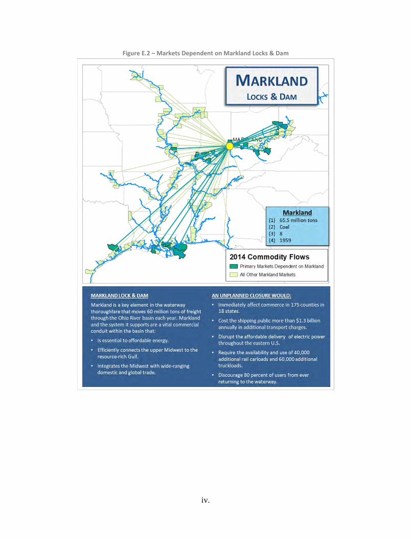
iv.
Figure E.2 – Markets Dependent on Markland Locks & Dam

v.
Figure E.3 – Markets Dependent on Calcasieu Lock

vi.
Figure E.4 – Markets Dependent on LaGrange Lock & Dam
vii.
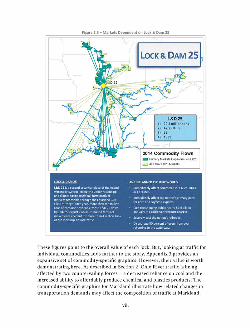
Figure E.5 – Markets Dependent on Lock & Dam 25
These figures point to the overall value of each lock. But, looking at traffic for individual commodities adds further to the story. Appendix 3 provides an expansive set of commodity-specific graphics. However, their value is worth demonstrating here. As described in Section 2, Ohio River traffic is being affected by two countervailing forces – a decreased reliance on coal and the increased ability to affordably produce chemical and plastics products. The commodity-specific graphics for Markland illustrate how related changes in transportation demands may affect the composition of traffic at Markland.

viii.
Figure E.6 – Distribution of Chemical Shipments Transiting Markland Locks & Dam
Figure E.7 – Distribution of Coal Shipments Transiting Markland Locks & Dam
Finally, the direct results described above were combined with a 2014 National Waterways Foundation analysis to estimate upper bounds for the regional

ix.
economic impacts associated with an unplanned lock closure. The regional impact – lost incomes and lost jobs –are summarized below.
Table E.2 – Estimated Regional Impacts Markland Calcasieu LaGrange UM L&D 25
Regional Output $2,520,578,383 $4,347,871,315 $5,188,761,521 $5,242,759,485 Regional Incomes $657,544,177 $1,094,959,385 $1,462,470,596 $1,570,516,397 Regional Employment 13,210 17,487 24,447 24,250
Note: These impacts cannot be summed across the four locks.
SUMMARY AND FINDINGS
The historical importance of the inland navigation system to the United States has been tied to the network’s coverage of the heartland and its efficient connectivity covering over 12,000 miles. This comes from the standardization of system capabilities, and especially the minimum channel depth and “standardization” of the more than 170 lock and dam structures, that allows the same equipment to efficiently traverse the entire system and from which the success of the system has been derived.
Unfortunately, the connectivity of the system also creates vulnerability, and this study documents and illustrates the magnitude of the impact from the prolonged loss of any single lock and dam project. If an unscheduled and extended outage were to occur at any of the four locks analyzed here, the impact would reach across all of the states served by the system and cause billions of dollars in economic harm to shippers, the commerce that depends on those shippers, and the communities that rely on this substantial business activity.
A FEW KEY FINDINGS
■ Each of the four locks considered within the study helps shippers avoid more than $1 Billion in additional transportation costs each year.
■ The important roles played by individual navigation projects span a broad range of both geographies and economic purposes, and in some cases provide freight mobility that could not be easily replaced by other transport modes.
■ While every state that originates or terminates traffic supported by the four locks benefits from inland navigation’s availability, the results reflect the waterway’s extraordinary commercial value to 18 states, especially Louisiana, Texas, and Illinois.
■ In the cases of LaGrange Lock & Dam and Lock & Dam 25, trucking to alternative waterway locations would mean an additional 500,000 loaded truck trips per year and an additional 150 million truck miles in the affected states. This is not tenable.

The Impacts of Unscheduled Lock Outages
Submitted to
The National Waterways Foundation and The U.S. Maritime Administration
by
Center for Transportation Research
The University of Tennessee
Vanderbilt Engineering Center for Transportation and Operational Resiliency
Vanderbilt University
October 2017

1.
Research Motivation, Context, and Approach The National Waterways Foundation (NWF) has partnered with the U.S. Department of Transportation’s Maritime Administration (MARAD) to sponsor this research project which estimates the specific economic consequences resulting from the unscheduled and extended closure of four
representative navigation locks. At each of the four locks selected, the impact on shippers currently using the locks, called the Shipper Supply Chain Cost Burden is estimated to exceed $1 billion per year with very significant additional regional economic and employment impacts extending widely over the territory served by the inland waterway system.
Through this work the sponsors also seek to demonstrate an analytical framework that can be applied to additional locks and in some contexts, measurably reduce the resources needed to undertake robust waterway system project evaluations.
1.1 PROJECT OVERVIEW AND APPROACH The more than 12,000 miles of navigable waterways in the U.S. are composed of segments with characteristics that vary considerably. On some segments of the system, like the lower Missouri and lower Mississippi Rivers, the combination of upstream water management and naturally occurring river flows allow for “open river” where barge traffic can move, unimpeded, from one end of the segment to the other. More commonly, however, maintaining dependable, year-long navigation requires the use of dams that help maintain acceptable channel depths within the pools they create. On these segments, passage around the necessary dams requires navigation locks that lift or lower vessels, including commercial towboats and barges, allowing them to pass from one pool to the next.
On waterway segments where dams and locks are necessary, any disruption in a lock’s operation can significantly inhibit barge transportation. In some cases, lock outages are scheduled to allow for necessary maintenance. These scheduled outages are announced months or even years in advance so that impacted waterway shippers can adjust commodity inventories or otherwise prepare for the service disruption. In other cases, however, weather, accidents, or mechanical failures lead to unscheduled lock closures of varying durations. Because carriers and shippers have no opportunity to prepare for unscheduled lock outages, these closures can be tremendously disruptive to water-dependent commerce. It is this latter type of outage on which the current work is focused.
1
2.
The overall effort has been divided into four broad sets of tasks:
■ The development of a methodology for selecting a small number of locks for careful analysis;
■ The collection and analysis of the data necessary to defensibly estimate the direct economic costs of the subject lock closures;
■ The extension of the direct closure-related costs to estimate the broader, economy-wide regional indirect impacts, and
■ The documentation of the approach to allow use of the methodology in future analyses.
Additionally, the study team was charged with using visualization tools that enhance the interpretation of the team’s analytical results. The sections that follow are organized around these goals.
Finally, while the topics and methods described here are anchored to rigorous economic and statistical principles, the research team has attempted to use a practical, applied approach suited for real-world practitioners.
1.2 REPORT STRUCTURE Chapter 2 provides the primary results that have been generated by this research effort. For each of the four locks selected for detailed analysis, tables and graphical representation summarize Shipper Supply Chain Cost Burden and the resulting regional economic impact that would result from an unanticipated closure of the analyzed lock and dam project. Chapter 2 concludes with an assessment of how rail capacity may impact these shipper costs.
Beyond developing the results for these four selected locks, an additional goal of the work reported here is to demonstrate efficient methods that will facilitate future project analyses. To that end, we include fairly detailed and technical descriptions of both data and methodologies. Chapters 3, 4, and 5 fully describe application of the data and existing tools used to screen and select locks, calculate the costs averted by preventing unscheduled lock closures, and estimate the regional economic impacts. Additional supporting material is provided in three Appendices.

3.
Study Methodology and Findings Lock Selection, Shipper Supply Chain Cost Burden Analysis, Regional Economic Impact Analysis The analytical path summarized in the introduction produced three specific products – a screening tool that was used by project sponsors to select four individual locks for further analysis, estimates of the supply chain costs that would be imposed directly on waterway users when unplanned lock
closures are not avoided, and estimates of subsequent regional impacts that extend the estimated closure costs to a broader set of economic effects. At the time that this project was begun in 2016, the most recent year for which complete data sets were available was 2014, and the reported findings are based on that year’s information. These findings and applications are summarized below.
2.1 LOCK SELECTION The screening tool described is a cross-sectional framework that compares fully disaggregated lock and dam infrastructure and performance characteristics to isolate navigation projects based on analytical purpose. For each lock, specific screening tool elements reflect:
■ Physical characteristics (e.g., age, number/dimensions of chambers);
■ Performance (e.g., tonnage, number of lockages, processing times); and
■ Network role (e.g., system ton-miles, and associated lockages at other locations).
The current work developed corresponding data for a population of 170 navigation locks. By design, the screening tool coalesces data that allow an array of cross-sectional comparisons of lock attributes, performance, and network functions. In the current application, the study team did not apply a weighting scheme that favors or reduces the importance of any particular lock characteristic. Instead, screening tool data were provided without any presupposed preferences.
Based on these data, the project sponsor evaluated a subset of the whole universe of locks and ultimately selected four facilities for further analysis. These include Markland Locks & Dam on the Ohio River, near Cincinnati; Calcasieu Lock on the Gulf Intracoastal Waterway in Louisiana; LaGrange Lock & Dam, the southern-most of the navigation structures on the Illinois River; and Lock & Dam 25 (L&D25) on the Mississippi River, immediately north of St. Louis. These four locations are depicted graphically in Figure 2.1. Chapter 3 more fully describes the lock selection criteria and process. However, generally, these locks were selected to reflect a solid cross-section of geography, commodity mix, and network role. Table 2.1 provides sample screening tool data for the four locks selected for further study.
2

4.
Table 2.1 – Screening Tool Results Summary
CALCASIEU LAGRANGE L&D 25 MARKLAND LOCK LOCATION INFORMATION
River GIWW ILLINOIS MISSISSIPPI OHIO
River Mile 238.5 80.2 241.4 531.5
Bank R R R L
USACE Division MVD MVD MVD LRD
USACE District MVN MVR MVS LRL
State LA IL MO KY
Town Lake Charles Beardstown Winfield Warsaw
Latitude 30.088061 39.94507 39.003117 38.774413
Longitude -93.293273 -90.53714 -90.689209 -84.966172
LOCK CHARACTERISTICS
Lift 4 10 15 35
Length 1205 600 600 1200
Width 75 110 110 110
Year Opened 1950 1939 1939 1959
Gate Type Sector Miter Miter Miter
Mooring Cells N N Y Y
AGGREGATE LOCK ACTIVITY
Lockages 3,987 3,659 3,172 4,071
LPMS Total Tons1 42,240,214 27,199,448 21,673,519 52,753,624
COMMODITY INFORMATION
WCSC Coal 245,836 443,288 660,624 30,788,869
WCSC Petroleum 24,988,887 5,623,494 320,411 7,440,371
WCSC Chemicals 9,078,337 4,888,770 4,171,737 3,898,264
WCSC Crude Materials 3,937,379 3,401,419 3,082,613 14,339,508
WCSC Primary Manufact. Prod. 2,744,157 3,344,289 1,667,149 4,896,902
WCSC Food and Farm Products 843,753 11,460,988 12,433,825 4,089,324
WCSC Machinery / Equipment 9,222 5,632 6,602 55,525
WCSC Waste Materials 626,896 - - -
WCSC Total Tons1 42,474,467 29,167,880 22,342,961 65,508,763
SYSTEM FUNCTIONS
System Ton-Miles Supported 2,330,362,699 35,764,883,159 29,499,570,937 48,278,194,662
Lockages per Barge 4.4 8.1 15.9 7.5
Total Tons - Pool Above 58,671 1,065,293 0 10,801,531
Total Tons - Pool Below 62,800 2,344,044 33,815 22,015,111
1 Limitations in LPMS data collection methods (particularly pertaining to coal movements) often lead to deviations between LPMS and WCSC-based tonnage values. In such cases, the WCSC figures are generally considered more reliable

5.
Figure 2.1 – Selected Lock Project Characteristics
2.2 SHIPPER SUPPLY CHAIN COST BURDEN (SSCCB) ANALYSIS At its core, the current project is intended to simulate and measure the direct economic costs of unanticipated navigation lock closures using existing data and tools in ways that reduce the resources required to undertake this type of analysis. Meeting this goal required the execution of three primary task sets that included:
■ Lock selection and data preparation; ■ Scenario design and traffic diversion assessments; and ■ The calculation of shipper supply chain costs both before and after an unanticipated lock
closure.
Lock Project Characteristics (1) Annual Tons (2) Primary Commodity (3) Lockages Per Barge (rounded up) (4) Year Opened

6.
As with all study elements and consistent with the Project Proposal, this work is designed to conform to the Principles & Guidelines (P&G) that govern the analysis of all federal inland navigation infrastructure projects by the United States Army Corps of Engineers (USACE).2
As noted, the study team estimated supply chain costs and navigation-related shipper cost burdens for unplanned outages at four individual locks. As expected, in terms of traffic and commercial function, LaGrange and L&D 25 are relatively similar. By contrast, Markland and Calcasieu differ from both each other and from the two upper Mississippi and Illinois River locks.
LaGrange and L&D 25 feature long-haul movements that consist mostly of down-bound corn and soybeans and up-bound fertilizer. Traffic at Markland is dominated by coal movements that are typically shorter in distance. However, the remaining Markland traffic is quite diverse, both in terms of commodities and shipment geographies. Finally, shipments through Calcasieu are somewhat shorter than Markland moves and often not even half the length of the shipments that transit LaGrange or Lock & Dam 25. Whereas, Markland is dominated by coal and LaGrange and L&D 25 are dominated by grain, Calcasieu traffic is primarily petroleum and chemical products.
These four locks support traffic on every segment of the Mississippi River system. Most of the traffic at LaGrange and L&D 25 flows the length of that main-stem and makes relatively lesser use of tributaries or intermediate terminal locations. By contrast, both the Ohio River coal traffic and, to a lesser degree, the traffic flows through Calcasieu routinely involve origins and destinations that are located along system tributaries or at intermediate spots between major terminal regions. To highlight this difference, the study team developed a Corridor Concentration Metric that combines data on traffic distributions with information describing shipment distances into a single measure called the Corridor Concentration Index. All else equal, a value closer to zero indicates that diverted shipments are less likely to face capacity constraints and a value closer to 1 signals the opposite, based both on the shipment distances and the limited number of available routes. The results of this calculation for the four subject locks are depicted in Figure 2.2. A shipper traversing a lock with a higher concentration metric score is more likely to face capacity issues in seeking to use alternative modes, especially rail, if lock operations are disrupted. This is more fully discussed in Section 2.4, and the data used and a discussion of the metric’s calculation are provided in Appendix 1.
Finally, while nearly every state that originates or terminates traffic supported by the four locks clearly benefits from inland navigation’s availability, analysis reflected the waterway’s extraordinary commercial value in Louisiana, Texas, and Illinois.
2 See Economic and Environmental Principles and Guidelines for Water and Related Land Resources Implementation Studies, Washington, DC, March 10, 1983.

7.
Figure 2.2 – Corridor Concentration Metrics
Markland Locks & Dam
The Shipper Supply Chain Cost Burden expected at Markland if an unscheduled closure of the lock were to occur is summarized in Table 2.2, and based on the 2014 data used in the study, the annual Cost Burden is estimated to exceed $1.3 billion.
The geographical distribution of this outcome is depicted in Figure 2.3. What is very clearly shown by the figure is that the impact of even a single lock closure can be system-wide and will be felt across the entire midsection of the United States. Appendix 3 provides similar graphics based on commodity-specific flows.
As noted in Section 2.1 (Lock Selection), the Markland traffic includes a substantial number of relatively short-haul coal movements that generally serve markets that are rail-competitive. While coal is the primary source of traffic volumes, both chemicals and petroleum products generate larger aggregate averted costs. Given the uncertainty of future coal volumes and the projected growth in chemical and plastics, this distinction is important. The distributions of current coal and chemical traffic that transits Markland are depicted graphically in Figures 2.4 and 2.5. The contrast is fairly striking.
The study-estimated 2014 tonnage at Markland, based on Waterborne Commerce Statistics Center (WCSC) data, is 12.8 million tons greater than the traffic volumes reported through the Lock Performance Monitoring System (LPMS). An examination of the commodity-specific values reveals that this variation is almost entirely attributable to differing values for coal. This sort of reporting differential is common to coal movements throughout the Ohio basin and is well-known to both the USACE and other transportation practitioners. Because the LPMS data sometimes depend on estimates by lock personnel who necessarily are focused principally on
L&D 25

8.
safe and expeditious vessel transits, the WCSC data more accurately capture instances of barge loadings to depths greater than 9 feet observed when river conditions allow.
Calcasieu Lock Located roughly halfway between Houston and Baton Rouge and immediately south of Lake Charles, Louisiana, the Calcasieu Lock is a critical element in inland navigation between Texas and Louisiana. The Shipper Supply Chain Cost Burden for Calcasieu is reported in Table 2.3 and depicted in Figure 2.6. In total, the cost burden is estimated to exceed $1.1 billion. Not surprisingly, traffic through the single-chamber lock is dominated by petroleum and chemical traffic that, together accounted for 80 percent of the project’s 2014 tons. The shorter shipment distances impact the per-ton cost. However, on a ton-mile basis, these costs are consistent with the values attained elsewhere. Appendix 3 provides similar graphics based on commodities.
A forward-looking regional view suggests measurable traffic growth in coming decades. In, 2015, Texas and Louisiana, together, accounted for nearly two-thirds of all U.S. investment in “mobile” manufacturing capital. Much of this reflects what the American Chemistry Council estimates to be $164 billion in new natural gas-related chemical and plastics investment.
LaGrange Lock & Dam and Lock & Dam 25 Volumes at LaGrange and at Lock & Dam 25 are dominated by Gulf-destined, down-bound flows of corn and soybeans. Ten million tons of farm products pass through each lock annually. The 20 million ton total is nearly six times greater than the volume of farm products moving by rail in the same corridor. In addition to down-bound corn and soybeans, both locks handle approximately four million tons of up-bound fertilizer annually. Finally, LaGrange tonnage also includes chemical, petroleum, and manufactured goods flows tied to commerce with origins and destinations along the Chicago Area Waterway System (CAWS).
The potential Shipper Supply Chain Cost Burden for grain passing through LaGrange and L&D 25 are large compared to corn and soybean movements elsewhere on the inland system. There are two reasons for this. First, below St. Louis, the Mississippi is open river, where tow sizes of 30 barges or more are common. Thus, total per ton barge charges are lower than elsewhere.
As important, both terminal capacity constraints and railroad line-haul capacities over relevant route segments suggest that, if forced from the river, most upper Mississippi and Illinois River basin corn and soybeans would divert to all-rail routings to locations in the Pacific Northwest (PNW).3 Railroad per-ton costs (to any location) are significantly higher than the cost of barge transportation to the Louisiana Gulf and the distance to the Pacific Northwest is generally twice the distance to Gulf export locations. Thus, even though cost estimates were offset to reflect ocean rate differentials to Pacific Rim destinations, the relatively high cost of rail diversions leads to high potential supply chain costs. The Shipper Supply Chain Cost Burden for a closure at LaGrange and Lock & Dam 25 is reported in Tables 2.4 and 2.5 and depicted in Figures 2.7 and 2.8. The total cost burden of an unplanned closure exceeds $1.5 billion at either lock.
3 While Canadian ports are not necessarily excluded, for the most part, use here to the “PNW” refers to West Coast locations in Oregon and Washington.

9.
Table 2.2 – Closure-Related Supply Chain Cost Burden, Markland Locks & Dam
LPMS Group Total 2014 Tons
Tons per Barge
Average Distance
Cost per Ton
Total Averted Costs
Coal 10 30,788,869 1,675 473 $7.21 $221,987,745 Petroleum Products 20 7,440,371 2,598 967 $49.49 $368,253,302 Chemicals 30 3,898,264 1,693 1,412 $70.91 $276,416,124 Crude Materials 40 14,339,508 1,673 757 $16.93 $242,729,791 Primary Manufactured Goods 50 4,896,902 1,658 1,294 $32.75 $160,394,481 Farm Products and Food 60 4,089,324 1,826 1,342 $9.41 $38,460,711 Equipment 70 55,525 1,586 1,216 $32.75 $1,818,681 TOTAL 65,508,763 $1,310,060,835
Table 2.3 – Closure-Related Supply Chain Cost Burden, Calcasieu Lock
LPMS Group
Total 2014 Tons
Tons per Barge
Average Distance
Cost per Ton
Total Averted Costs
Coal 10 245,836 1,617 1,268 $26.97 $6,629,552 Petroleum Products 20 24,988,887 2,859 542 $21.70 $542,287,348 Chemicals 30 9,078,337 2,022 846 $25.44 $230,953,087 Crude Materials 40 3,937,379 1,578 1,230 $45.66 $179,789,257 Primary Manufactured Goods 50 2,744,157 1,568 1,114 $43.73 $120,009,771 Farm Products and Food 60 843,753 1,769 1,021 $26.97 $22,753,806 Equipment 70 9,222 307 524 $26.97 $248,693 Scrap and Waste 80 626,896 1,537 259 $26.97 $16,905,741 TOTAL 42,474,467 $1,119,577,255
Table 2.4 – Closure-Related Supply Chain Cost Burden, LaGrange Lock & Dam
LPMS Group
Total 2014 Tons
Tons per Barge
Average Distance
Cost per Ton
Total Averted Costs
Coal 10 443,288 1,566 942 $45.77 $20,291,015 Petroleum Products 20 5,623,494 2,210 1,202 $32.53 $182,914,135 Chemicals 30 4,888,770 1,739 1,230 $51.45 $251,529,491 Crude Materials 40 3,401,419 1,552 1,270 $61.22 $208,236,345 Primary Manufactured Goods 50 3,344,289 1,513 1,056 $30.96 $103,524,351 Farm Products and Food 60 11,460,988 1,588 1,226 $81.38 $932,684,606 Equipment 70 5,632 704 1,416 $84.87 $477,986 TOTAL 29,167,880 $1,699,657,929
Table 2.5 – Closure-Related Supply Chain Cost Burden, Lock & Dam 25
LPMS Group
Total 2014 Tons
Tons per Barge
Average Distance
Cost per Ton Total Averted Costs
Coal 10 660,624 1,547 713 $38.90 $25,696,959 Petroleum Products 20 320,411 1,732 1,518 $47.14 $15,103,646 Chemicals 30 4,171,737 1,612 1,430 $59.66 $248,899,601 Crude Materials 40 3,082,613 1,568 1,488 $67.76 $208,863,996 Primary Manufactured Goods 50 1,667,149 1,677 845 $22.93 $38,225,955 Farm Products and Food 60 12,433,825 1,598 1,323 $83.16 $1,033,977,564 Equipment 70 6,602 660 1,270 $82.19 $542,606 TOTAL 22,342,961 $1,571,310,327

11.

11.
Figure 2.4 – Distribution of Chemical Shipments Transiting Markland Locks & Dam4
Figure 2.5 – Distribution of Coal Shipments Transiting Markland Locks & Dam
4 These graphics are provided to emphasize the potential change in Ohio River traffic composition. Similar depictions for an array of commodities and encompassing all four locks can be found in Appendix 3.

12.
Figure 2.6 – Markets Dependent on Calcasieu Lock5
5 Depictions similar to that provided for Markland for Calcasieu commodities can be found in Appendix 3.

13.
Figure 2.7 – Markets Dependent on LaGrange Lock & Dam6
6 Depictions similar to that provided for Markland for LaGrange commodities can be found in Appendix 3.

14.
Figure 2.8 – Markets Dependent on Lock & Dam 257
7 Depictions similar to that provided for Markland for Lock & Dam 25 commodities can be found in Appendix 3.

15.
2.3 REGIONAL ECONOMIC DEVELOPMENT (RED) ANALYSIS Consistent with the overarching goal to use existing resources more efficiently, results from a prior National Waterways Foundation sponsored-study were used to expedite the estimation of regional economic impacts for the four subject locks.8 Section 5 describes the specific steps necessary to this application. The earlier NWF work involved converting lock-related efficiencies into production cost advantages that were used as drivers in economic simulations. Here, we combine the earlier study results with current estimates of avoided transportation costs to estimate upper bounds for regional economic impacts (output, incomes, and employment) attributable to the subject locks. Note “output” refers to the total value of all regional sales. These estimates are combined with an alternative methodology to estimate a corresponding lower bound for the same impacts. It is the midpoint or average for each estimated outcome that is reported here.
Before presenting the results of these estimations, it’s useful to consider three points. First, even though there is often an overlap, economic benefits and economic impacts are not the same thing. Economic benefits are the net efficiency gains for which there is no offset. In this case these gains are the transportation costs avoided by ensuring reliable navigation infrastructures. Economic impacts are different. While they do account for the improved efficiency (direct effects), regional impacts also capture the ways that an economic improvement affects production, jobs, and incomes within a specific study area. These additional impacts often reflect economic transfers from one region to another. Nonetheless, they are a very real economic result of improved transportation access.
Next, calculating economic impacts requires an understanding of where a direct stimulus is likely to have its effects. It’s easy to understand that a cost-constraining navigation project physically located in a remote rural location will not materially affect economic conditions in the region surrounding the lock. However, it’s more difficult to determine where the direct effects will be felt. In response, the current analysis (and the earlier NWF-sponsored work) makes a strong simplifying assumption. In estimating regional economic impacts, the analysis assumes that for all non-farm product commodities, the economic stimulus associated with avoided transportation costs is divided equally between the region where the waterway shipment originates and the region where it terminates. As further explained in Section 5, this assumption is not tenable for farm products. Consequently, in the case of this commodity group, all direct effects are assumed to occur in the originating region.
Finally, unlike large-scale feasibility studies, this study does not adopt a systems approach, but instead examines each subject lock in isolation. For the estimated regional economic impacts, this methodology means that the results are not additive. Any attempt to sum effects across locks would result in double-counting.
8 INLAND NAVIGATION IN THE UNITED STATES: An Evaluation of Economic Impacts and the Potential Effects of Infrastructure Investment, National Waterways Foundation, November 2014, http://www.nationalwaterwaysfoundation.org/documents/INLANDNAVIGATIONINTHEUSDECEMBER2014.pdf

16.
Markland Locks & Dam - Table 2.6 provides estimates of the economic impacts tied to the commercial use of Markland. These values reflect the importance of Markland as a means of shuttling Kentucky coal mid-Ohio basin power plants, but they also document economic activity generated in Louisiana by a lock so far upstream, due to the ability to affordably move chemicals and petroleum from manufacturing and refining facilities on the Gulf to the upper Ohio basin. Regional employment effects of Markland are shown in Figure 2.9.
Table 2.6 – Economic Impacts Attributable to Markland Locks & Dam
Figure 2.9 – Regional Employment Effects of Markland Locks & Dam
StateTotal Avoided
Costs Total Attributable
Output Total Attributable
Incomes Total Attributable
EmploymentAL 4,504,940 10,742,105 2,693,298 49 AR 6,474,484 16,184,170 5,185,339 81 FL 163,962 558,126 135,933 2 IA 814,055 2,033,786 650,840 10 IL 42,622,718 90,346,646 27,064,511 463 IN 78,141,984 115,728,190 31,296,844 719 KY 326,983,504 470,449,884 125,966,921 3,008 LA 257,103,456 853,703,317 206,841,402 3,240 MN 634,116 1,671,426 530,007 8 MO 14,157,717 36,993,878 11,669,365 177 MS 3,208,111 5,954,770 1,455,911 30 OH 264,459,882 401,523,540 109,226,097 2,433 OK 5,012,705 9,548,722 2,363,199 47 PA 65,205,206 98,410,103 26,584,599 600 TN 7,960,054 12,267,476 3,324,682 73 TX 37,597,321 131,395,819 31,967,086 474 WI 96,643 246,196 79,088 1 WV 194,919,978 262,820,230 70,509,053 1,793
TOTAL $1,310,060,835 $2,520,578,383 $657,544,177 13,210 * Output is the total value of all regional sales.
*

17.
* Output is the total value of all regional sales.
Calcasieu Lock - Calcasieu Lock is an essential component in a conduit that links oil refining and chemical manufacturing facilities in Texas with similar operations in Louisiana and other locations along the Gulf-Intracoastal Waterway. Thus, it is not surprising that Texas and Louisiana rank first and second in economic activity summarized in Table 2.7. Notably, however, Illinois ranks third in terms of Calcasieu’s economic impacts. This importance, as it impacts regional employment, is depicted in Figure 2.10.
Table 2.7 – Economic Impacts Attributable to Calcasieu Lock
Figure 2.10 – Regional Employment Impacts Attributable to Calcasieu Lock
StateTotal Avoided
Costs Total Attributable
Output Total Attributable
Incomes Total Attributable
EmploymentAL 42,888,109 132,913,445 33,324,529 608 AR 33,118,475 107,593,798 34,472,595 515 FL 3,815,650 16,880,611 4,111,323 66 IA 764,635 2,482,772 794,522 12 IL 79,201,353 218,190,142 65,361,690 1,108 IN 33,631,545 64,734,109 17,506,308 394 KY 29,271,965 54,735,745 14,655,957 337 LA 283,789,119 1,224,690,717 296,726,908 4,554
MN 15,751,393 53,959,619 17,110,536 255 MO 26,871,911 91,257,134 28,786,190 436 MS 25,072,671 60,485,023 14,788,285 299 OH 12,189,517 24,053,005 6,543,118 151 OK 4,172,954 10,331,143 2,556,840 50 PA 15,370,275 30,148,846 8,144,438 180 TN 5,463,483 10,943,102 2,965,756 66 TX 486,123,401 2,208,018,996 537,185,533 8,236 WI 828,422 2,742,786 881,099 13 WV 19,236,622 33,710,319 9,043,758 209
TOTAL $1,117,561,501 $4,347,871,315 $1,094,959,385 17,487
*
18.
* Output is the total value of all regional sales.
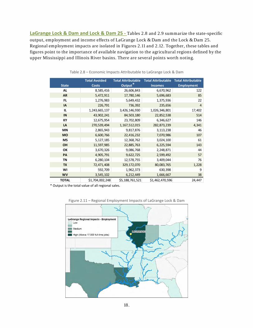
LaGrange Lock & Dam and Lock & Dam 25 - Tables 2.8 and 2.9 summarize the state-specific output, employment and income effects of LaGrange Lock & Dam and the Lock & Dam 25. Regional employment impacts are isolated in Figures 2.11 and 2.12. Together, these tables and figures point to the importance of available navigation to the agricultural regions defined by the upper Mississippi and Illinois River basins. There are several points worth noting.
Table 2.8 – Economic Impacts Attributable to LaGrange Lock & Dam
Figure 2.11 – Regional Employment Impacts of LaGrange Lock & Dam
StateTotal Avoided
Costs Total Attributable
Output Total Attributable
Incomes Total Attributable
EmploymentAL 8,585,416 26,606,843 6,670,962 122 AR 5,472,911 17,780,146 5,696,683 85 FL 1,276,983 5,649,432 1,375,936 22 IA 226,791 736,392 235,656 4 IL 1,243,665,137 3,426,146,930 1,026,346,801 17,402 IN 43,902,241 84,503,180 22,852,538 514 KY 12,675,954 23,702,809 6,346,627 146 LA 270,539,494 1,167,512,015 282,873,239 4,341
MN 2,865,943 9,817,876 3,113,238 46 MO 6,600,766 22,416,232 7,070,986 107 MS 5,127,185 12,368,762 3,024,100 61 OH 11,597,985 22,885,763 6,225,594 143 OK 3,670,326 9,086,768 2,248,871 44 PA 4,905,791 9,622,725 2,599,492 57 TN 6,280,104 12,578,755 3,409,044 76 TX 72,471,408 329,172,070 80,083,765 1,228 WI 592,709 1,962,373 630,398 9 WV 3,545,102 6,212,449 1,666,667 38
TOTAL $1,704,002,248 $5,188,761,521 $1,462,470,596 24,447
*

19.
* Output is the total value of all regional sales.
Table 2.9 – Economic Impacts Attributable to Lock & Dam 25
Figure 2.12 – The Regional Employment Impacts of Lock & Dam 25
First, as mentioned above, in the case of farm products, the whole of the economic impacts are assumed to reside in the origin regions. Also, as described in Section 2.4, the likely diversion of current waterborne shipments of corn and soybeans to the PNW would increase transportation costs significantly above present levels. Together, these combined influences predict a fairly dramatic decline in farm incomes within both river basins, with attendant indirect and induced impacts throughout the region.
StateTotal Avoided
Costs Total Attributable
Output Total Attributable
Incomes Total Attributable
EmploymentAL 2,793,743 8,658,018 2,170,769 40 AR 6,801,464 22,096,288 7,079,557 106 FL - - - - IA 369,628,309 1,200,184,825 384,076,031 5,763 IL 340,595,456 938,299,258 281,079,727 4,766 IN 2,812,857 5,414,196 1,464,183 33 KY 2,371,176 4,433,870 1,187,206 27 LA 211,309,773 911,906,412 220,943,268 3,391
MN 379,834,042 1,301,199,232 412,608,844 6,147 MO 130,893,626 444,515,357 140,218,116 2,123 MS 4,737,495 11,428,678 2,794,254 56 OH 2,182,266 4,306,163 1,171,402 27 OK 2,073,890 5,134,410 1,270,708 25 PA 848,134 1,663,618 449,411 10 TN 1,253,866 2,511,435 680,639 15 TX 24,780,404 112,554,967 27,383,324 420 WI 79,374,813 262,798,466 84,422,032 1,266 WV 3,226,594 5,654,293 1,516,926 35
TOTAL $1,565,517,907 $5,242,759,485 $1,570,516,397 24,250
*
20.
However, even though down-bound grain is assumed to have no effect on the Louisiana Gulf economy, the effects of LaGrange and of L&D 25 are still pronounced in Louisiana (19 percent of the total for LaGrange, 14 percent of the total for L&D 25). Based on commodity disaggregations of the subject traffic, these impacts are almost exclusively attributable to the waterways’ ability to constrain costs for up-bound movements of chemicals and petroleum products.
2.4 RAILROAD CAPACITY AND ITS IMPACT ON SHIPPER COSTS There are several complexities that lie just below the surface of the navigation-attributable averted costs summarized in Section 2.2. Some of these are addressed by the P&G, but rarely treated in application. Other intricacies lie outside the P&G’s normal bounds.
The basic questions are:
1. To the extent that railroads and rail-served terminals would be expected to absorbdiverted waterway traffic, do they have the capacity to accommodate the additionaldemands?
2. If capacity is inadequate, would the railroads and terminal operators invest in newcapacity to support the same routes currently used by waterway shippers?
3. If, instead of adding new capacity, traffic is diverted to alternative locations wheretransportation costs are higher, are those higher costs appropriately included in thecalculation of navigation related benefits?
4. How do time horizons and uncertainty about modal availability affect the answers to thefirst three questions?
The P&G and Capacity With regard to the issue of capacity, the P&G (2.6.3 (a) 4, p. 50) state:
In projecting traffic movements on other modes (railroad, highway, pipeline, or other), the without-project condition normally assumes that the alternative modes have sufficient capacity to move traffic at current rates unless there is specific evidence to the contrary.
Based on this guidance, USACE studies almost always assume that alternative modes or modal combinations have capacities that are sufficient to accommodate diverted traffic. When capacity has emerged as a potential issue, the assumption has been that it can be added without adversely affecting prevailing freight rates. In either case, this allows analysts to rely on currently observed values and relieves any need to estimate the cost of additional capacity or the extent to which those costs might affect project benefit calculations.
Where and Why Is Capacity an Issue? As noted, unless there is evidence to the contrary, the methods used to estimate averted shipper costs presume that there is transport capacity available from the other primary freight modes – truck and rail – to absorb the additional volumes presented as a result of the individual lock closure.
21.
After reviewing the mix of commodities, transportation alternatives, and the pattern of origins and destinations that determine corridor concentration and length of haul, rail capacity does not appear to be an issue for Markland or Calcasieu traffic. In the cases of LaGrange and L&D 25, however, it appears that the capacity assumption is inappropriate and, if left treated, may lead to an understatement of the shipper costs that would result from an unplanned lock closure.
One useful way to illustrate why this concern is present at LaGrange and L&D 25 but less so at Markland and Calcasieu is to further examine the traffic concentration and length of haul. Figures 2.13 and 2.14 reflect the traffic concentration of the four locks and again illustrate that traffic flows through both L&D 25 and LaGrange are concentrated along north-south corridors and feature a line-haul that routinely extends more than a thousand miles.9 Alternatively, Calcasieu (to some degree) and Markland (in particular) serve traffic in many corridors, with trip distances that are only 60 percent as long for LaGrange and L&D 25. Where it exists, this concentration of waterway traffic into narrowly-defined, heavy-haul corridors has implications regarding the adequacy of both line-haul and terminal capacities.
Line-Haul Railroad Capacity Issues Currently, LaGrange and L&D 25 support the movement of roughly 10 million tons each of corn and soybeans from the upper Mississippi and Illinois basins to export locations at or near New Orleans (the Louisiana Gulf). This grain is produced on farmland that has no meaningful alternative use. Even in the event of long-term decline in farm incomes and further restructuring to regional agriculture, there is no reason to suppose that a reduction in agricultural production would take place.
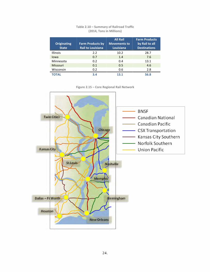
Table 2.10 summarizes current (2014) railroad movements from potentially affected upper basin states to the Louisiana Gulf. Figure 2.15 depicts the rail network serving those regions. Looking first at the data, it is clear that any attempt to substitute rail for barge toward the movement of 10 million additional down bound tons would represent a significant increase in north-south railroad traffic. LaGrange and L&D 25 both provide extreme evidence of potential congestion.
Virtually all waterway movements of corn and soybeans through LaGrange originate in Illinois, so that an unplanned lock outage would leave 10 million tons of corn and soybeans seeking a south bound routing along corridors that currently accommodate only 2.2 million tons of farm products annually.10
Grain movements through L&D 25 have more geographically dispersed origins that would allow a wider variety of potential line-haul routings. However, the percentage increase in southbound traffic would be even greater, with 10 million tons seeking movement along rail corridors that currently accommodate only 1.2 million tons of farm products annually.
9 The stylized (green) corridors are based on the study team’s examination of the data used to generate the Corridor Concentration Index described in Section 2 and Appendix 1. 10 The 2.2 million ton total is the total volume of soybeans and corn railed from Illinois, Iowa, Minnesota, Missouri, and Wisconsin to export locations in Louisiana as indicated through the Surface Transportation Board’s 2014 Annual Carload Waybill Sample.

22.
Figure 2.13 – Corridors Served by Markland and Calcasieu
Low
Medium
High
Low
Medium
High

23.
Figure 2.14 – Corridors Served by LaGrange and L&D 25
Low
Medium
High
Low
Medium
High
Primary Corridors
24.
Table 2.10 – Summary of Railroad Traffic (2014, Tons in Millions)
Originating State
Farm Products by Rail to Louisiana
All Rail Movements to
Louisiana
Farm Products by Rail to all Destinations
Illinois 2.2 10.2 28.7 Iowa 0.7 1.4 7.6 Minnesota 0.2 0.4 13.1 Missouri 0.1 0.5 4.6 Wisconsin 0.2 0.6 2.8 TOTAL 3.4 13.1 56.8
Figure 2.15 – Core Regional Rail Network
.

25.
Routing an additional 10 million tons to any location would require additional locomotives, covered hoppers, train crews, and track capacity. It would also require the use of nonexistent railroad capacity at many originating and destination terminal facilities. Setting aside the terminal issues for a moment, line-haul implications are relatively easy to explore.
Table 2.11 converts 10 million tons of additional annual demand for corn and soybean transport into line-haul railroad system characteristics based on an unplanned outage at LaGrange. Given current conditions, the equipment required to meet this additional demand is available. Data shows that presently there are more than 60,000 covered hoppers in storage. Similarly, both Union Pacific and BNSF have each stored hundreds of readily serviceable locomotives. Thus, under current conditions equipment is not an issue. However as recently as 2014, both locomotives and appropriate freight cars were much scarcer.
Again, almost without regard to export destination, the addition of the trains needed to accommodate a 10-million-ton increase would require between 200 and 300 additional qualified crew members. In some instances, displaced crews from unaffected locations could be expected to qualify and bid for jobs along affected routes. In other cases, it would be necessary to hire altogether new personnel to fill newly-created vacancies. Any attempt to accommodate the demands resulting from an unplanned lock closure through increased rail carriage could create at least temporary labor shortages.
In the case of LaGrange, both the Canadian National and Union Pacific could accommodate some of the incremental line-haul traffic. Doing so would require between three and four loaded trains originating toward the south each day and a corresponding number of originating north bound empties. Assuming that this traffic could be split between the two carriers, each affected segment of the railroad would see an additional three or four trains per day. Over the least active route segments, this would likely represent an immediate and unrelenting increase of train activity of roughly 25 percent.
In the end, any attempt to accommodate an unanticipated lock outage at LaGrange through the increased movement of corn and soybeans between Illinois and the Louisiana Gulf would place significant line-haul stresses on the Canadian National and Union Pacific Railroads. While it is likely that both carriers could adjust to accommodate the measurable increases in demand, doing so would not be accomplished quickly, easily, or without disruption to more general operations throughout the rail system.
An unanticipated outage at L&D 25 would present similar challenges with some important variations. On the positive side, the more westerly upstream origins for south bound corn and soybean movements would perhaps allow BNSF to play a larger role in addressing the sudden new demands. Unfortunately, the transit distance between most Iowa, Minnesota and Wisconsin origins are considerably longer than LaGrange-dependent traffic. Moreover, in some cases, traffic diverted to rail would necessarily transit Chicago, so that the car cycle times indicated for LaGrange would likely be much longer for L&D 25 movements.

26.
Table 2.11 – Illustrative Rail System Impacts, LaGrange Outage
Railroad System Impacts
Additional Annual Tons from LaGrange 10,000,000 Average Car Loading (Tons) 112 Additional Annual Carloads 89,286 Average Car Cycle Time (Days) 21 Annual Cycles 17 Additional Freight Cars (Continuous) 5,208 Train Length (Cars) 80 Additional Daily System Trains (Loads & MTYS) 65 Locomotives per Consist 2.5 Additional Locomotives 163 Average RR Distance (Miles) 1,000 Daily Trains per 100 Mile Track Length 7
LaGrange, L&D 25 and Terminal Capacity Issues Potential line-haul congestion issues likely pale in magnitude compared to the constraints that exist at the terminal ends of diverted waterway movements. At least some Louisiana Gulf grain terminals have only modest rail access; some have no rail access at all; and a significant volume of corn and soybeans are loaded to ocean-going vessels via mid-stream transfer, thereby avoiding downstream terminals altogether.
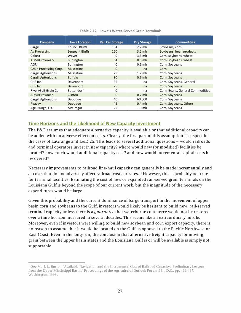
There are also possible terminal constraints at the origination end of Gulf-bound shipments of corn and soybeans. However, these limitations may not be as severe as the constraints faced at Louisiana Gulf destinations. Table 2.12 provides the characteristics of Iowa’s water-served grain terminals. While these characteristics are not necessarily descriptive of off-river terminals, they suggest that rail car capacity is an issue.
Finally, if necessary, new export grain terminal capacity can be created in the upper Mississippi and Illinois basin, on the Louisiana Gulf, or anywhere else it is desired. However, creating this capacity would require substantial private sector investment. Within the current context, new investments in terminal track capacities at the basin states origins would only be predicted as a response to extended lock closures. Further, in the case of export terminals, new alternative rail-served capacity is only likely if there is a permanent closure of either LaGrange or L&D 25 or if there are significant and lasting changes in the global markets these terminals serve.
27.
Table 2.12 – Iowa’s Water-Served Grain Terminals
Company
Iowa Location
Rail Car Storage
Dry Storage
Commodities
Cargill Council Bluffs 104 2.2 mb Soybeans, corn Ag Processing Sergeant Bluffs 250 3.5 mb Soybeans, bean products Colusa Wever 0 3.5 mb Corn, soybeans, wheat ADM/Growmark Burlington 54 0.5 mb Corn, soybeans, wheat AGRI Burlington 0 0.6 mb Corn, Soybeans Grain Processing Corp. Muscatine 0 na Corn Cargill AgHorizons Muscatine 25 1.2 mb Corn, Soybeans Cargill AgHorizons Buffalo 30 0.9 mb Corn, Soybeans CHS Inc. Davenport 35 na Corn. Soybeans, General CHS Inc. Davenport 25 na Corn, Soybeans River/Gulf Grain Co. Bettendorf 0 na Corn, Beans, General Commodities ADM/Growmark Clinton 0 0.7 mb Corn, Soybeans Cargill AgHorizons Dubuque 40 60,000 Corn, Soybeans Peavey Dubuque 45 0.4 mb Corn, Soybeans, Others Agri-Bunge, LLC McGregor 25 1.0 mb Corn, Soybeans
Time Horizons and the Likelihood of New Capacity Investment The P&G assumes that adequate alternative capacity is available or that additional capacity can be added with no adverse effect on costs. Clearly, the first part of this assumption is suspect in the cases of LaGrange and L&D 25. This leads to several additional questions – would railroads and terminal operators invest in new capacity? where would new (or modified) facilities be located? how much would additional capacity cost? and how would incremental capital costs be recovered?
Necessary improvements to railroad line-haul capacity can generally be made incrementally and at costs that do not adversely affect railroad costs or rates.11 However, this is probably not true for terminal facilities. Estimating the cost of new or expanded rail-served grain terminals on the Louisiana Gulf is beyond the scope of our current work, but the magnitude of the necessary expenditures would be large.
Given this probability and the current dominance of barge transport in the movement of upper basin corn and soybeans to the Gulf, investors would likely be hesitant to build new, rail-served terminal capacity unless there is a guarantee that waterborne commerce would not be restored over a time horizon measured in several decades. This seems like an extraordinary hurdle. Moreover, even if investors were willing to build new soybean and corn export capacity, there is no reason to assume that it would be located on the Gulf as opposed to the Pacific Northwest or East Coast. Even in the long-run, the conclusion that alternative freight capacity for moving grain between the upper basin states and the Louisiana Gulf is or will be available is simply not supportable.
11 See Mark L. Burton “Available Navigation and the Incremental Cost of Railroad Capacity: Preliminary Lessons from the Upper Mississippi Basin,” Proceedings of the Agricultural Outlook Forum 98, , D.C., pp. 431-437, Washington, 1998.
28.
The Effect of a Lock Closure on Rail Charges for Export Soybeans and Corn Using a short-run time horizon, a recent United States Department of Agriculture (USDA) study acts upon the same conclusions regarding capacity. The USDA analysis considered similar disruptions at LaGrange and L&D 25.12 It concluded that roughly 60 percent of the waterway grain that currently is exported through the Louisiana Gulf would divert to rail carriage and be bound for alternative export destinations – primarily the Pacific Northwest. Moreover, in the USDA work, this diversion is bolstered by hypothetical rail rate increases to Gulf destinations of five and 15 percent. Based on our computations, the magnitudes of the USDA study’s diversions appear reasonable, though depending on terminal capacities, they may reflect a lower bound.
Based on this study’s analysis of railroad capacity, as well as findings provided in the USDA study, it appears that an unscheduled lock outage would divert a substantial portion of corn and soybeans from their current Louisiana Gulf export destinations to Pacific Northwest gateways. The estimated railroad charges associated with these PNW diversions are notably higher than existing rail charges to Gulf export locations. However, rates on the modest amount of corn and soybeans currently moving to the Louisiana Gulf by rail were not changed. These currently observed rail rates were also applied to the subset of currently waterborne corn and soybean shipments that were allowed Gulf coast diversions.
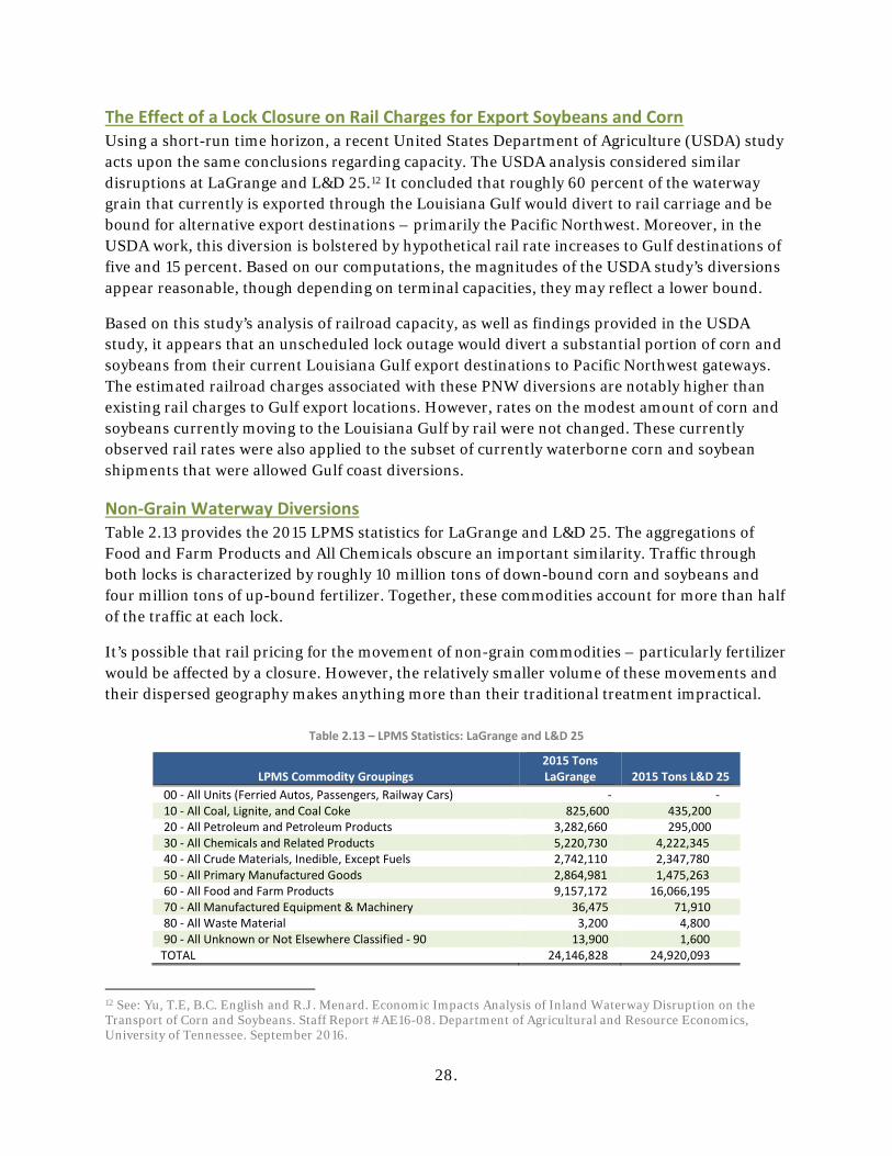
Non-Grain Waterway Diversions Table 2.13 provides the 2015 LPMS statistics for LaGrange and L&D 25. The aggregations of Food and Farm Products and All Chemicals obscure an important similarity. Traffic through both locks is characterized by roughly 10 million tons of down-bound corn and soybeans and four million tons of up-bound fertilizer. Together, these commodities account for more than half of the traffic at each lock.
It’s possible that rail pricing for the movement of non-grain commodities – particularly fertilizer would be affected by a closure. However, the relatively smaller volume of these movements and their dispersed geography makes anything more than their traditional treatment impractical.
Table 2.13 – LPMS Statistics: LaGrange and L&D 25
LPMS Commodity Groupings 2015 Tons LaGrange 2015 Tons L&D 25
00 - All Units (Ferried Autos, Passengers, Railway Cars) - - 10 - All Coal, Lignite, and Coal Coke 825,600 435,200 20 - All Petroleum and Petroleum Products 3,282,660 295,000 30 - All Chemicals and Related Products 5,220,730 4,222,345 40 - All Crude Materials, Inedible, Except Fuels 2,742,110 2,347,780 50 - All Primary Manufactured Goods 2,864,981 1,475,263 60 - All Food and Farm Products 9,157,172 16,066,195 70 - All Manufactured Equipment & Machinery 36,475 71,910 80 - All Waste Material 3,200 4,800 90 - All Unknown or Not Elsewhere Classified - 90 13,900 1,600 TOTAL 24,146,828 24,920,093
12 See: Yu, T.E, B.C. English and R.J. Menard. Economic Impacts Analysis of Inland Waterway Disruption on the Transport of Corn and Soybeans. Staff Report #AE16-08. Department of Agricultural and Resource Economics, University of Tennessee. September 2016.
29.
Screening Tool Development The purpose of the screening tool was to select locks on the inland waterway system that represent a balanced, cross-section. Section 2.1 summarizes the results of the current study’s screening tool construction and application and these results are more fully provided in Appendix 2..
3.1 FREIGHT DATA AND DATA ACCESS Compared to other industries, freight transportation data is plentiful. While each data product has limitations, access to and the use of these data is critical in this study and will be equally important for others who replicate these methods. The three most important data elements are:
■ Lock Performance Monitoring System (LMPS) data; ■ Waterborne Commerce Statistical Center (WCSC) data; and ■ The Surface Transportation Board’s annual Carload Waybill (CWS) data13
Lock Performance Monitoring System (LPMS) Data Each time a vessel transits a navigation lock, lock personnel log its passage and record a variety of data describing the specific lock operation, the vessel, and the vessel’s contents. This information is collected, processed and made available by the USACE’s National Data Center (NDC) as a part of its Lock Performance Monitoring System (LPMS).
The chief advantage of the LPMS data is that they are available quickly – usually with only a three-month lag. There are two primary limitations. First, LPMS data are only available for locations where the USACE operates navigation facilities. There is no corresponding set of information for reaches of open river. Second, tonnage information is estimated by the towboat operators transiting the locks and are not subject to verification.
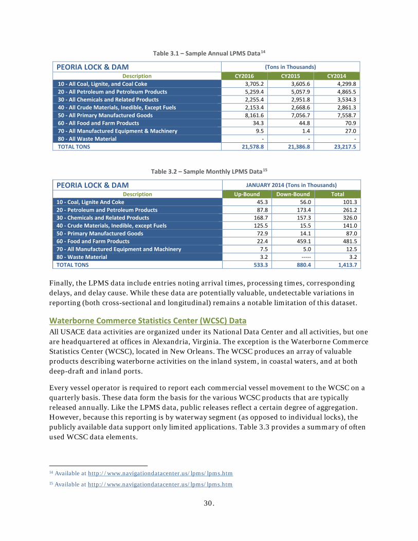
The LPMS data are publicly released at a level of disaggregation that is sufficient for many analytical uses. Table 3.1 provides a sample of the publicly available summary for one navigation lock (Peoria Lock) for 2014-2016. As Table 3.2 illustrates, these same data are available on a monthly basis by direction (up-bound v. down-bound) from 1999 forward.
13 The screening tool development described here did not use data from the CWS. However, it was used extensively in the evaluation of shipper supply chain costs described in Section 4. Moreover, from an organizational standpoint it seemed more sensible to describe all three primary data sources within a single subsection. This screening tool can be used by others who may wish to study additional locks on the inland waterway system.
3
30.
Table 3.1 – Sample Annual LPMS Data14
PEORIA LOCK & DAM (Tons in Thousands) Description CY2016 CY2015 CY2014
10 - All Coal, Lignite, and Coal Coke 3,705.2 3,605.6 4,299.8 20 - All Petroleum and Petroleum Products 5,259.4 5,057.9 4,865.5 30 - All Chemicals and Related Products 2,255.4 2,951.8 3,534.3 40 - All Crude Materials, Inedible, Except Fuels 2,153.4 2,668.6 2,861.3 50 - All Primary Manufactured Goods 8,161.6 7,056.7 7,558.7 60 - All Food and Farm Products 34.3 44.8 70.9 70 - All Manufactured Equipment & Machinery 9.5 1.4 27.0 80 - All Waste Material - - - TOTAL TONS 21,578.8 21,386.8 23,217.5
Table 3.2 – Sample Monthly LPMS Data15
PEORIA LOCK & DAM JANUARY 2014 (Tons in Thousands) Description Up-Bound Down-Bound Total
10 - Coal, Lignite And Coke 45.3 56.0 101.3 20 - Petroleum and Petroleum Products 87.8 173.4 261.2 30 - Chemicals and Related Products 168.7 157.3 326.0 40 - Crude Materials, Inedible, except Fuels 125.5 15.5 141.0 50 - Primary Manufactured Goods 72.9 14.1 87.0 60 - Food and Farm Products 22.4 459.1 481.5 70 - All Manufactured Equipment and Machinery 7.5 5.0 12.5 80 - Waste Material 3.2 ----- 3.2 TOTAL TONS 533.3 880.4 1,413.7
Finally, the LPMS data include entries noting arrival times, processing times, corresponding delays, and delay cause. While these data are potentially valuable, undetectable variations in reporting (both cross-sectional and longitudinal) remains a notable limitation of this dataset.
Waterborne Commerce Statistics Center (WCSC) Data All USACE data activities are organized under its National Data Center and all activities, but one are headquartered at offices in Alexandria, Virginia. The exception is the Waterborne Commerce Statistics Center (WCSC), located in New Orleans. The WCSC produces an array of valuable products describing waterborne activities on the inland system, in coastal waters, and at both deep-draft and inland ports.
Every vessel operator is required to report each commercial vessel movement to the WCSC on a quarterly basis. These data form the basis for the various WCSC products that are typically released annually. Like the LPMS data, public releases reflect a certain degree of aggregation. However, because this reporting is by waterway segment (as opposed to individual locks), the publicly available data support only limited applications. Table 3.3 provides a summary of often used WCSC data elements.
14 Available at http://www.navigationdatacenter.us/lpms/lpms.htm 15 Available at http://www.navigationdatacenter.us/lpms/lpms.htm

31.
Table 3.3 – Base WCSC Data Record Contents
Field No.
Variable Name
Description
Variable Type
1 REFNO Team-assigned reference number N 2 OFIPS Origin state/county FIPS code N 3 OST Origin state (alpha) A 4 OLAT Origin latitude N 5 OLON Origin Longitude N 6 OZIP Origin ZIP Code N 7 TFIPS Destination state/county FIPS code N 8 TST Destination state (alpha) A 9 TLAT Destination latitude N
10 TLON Destination longitude N 11 TZIP Destination ZIP Code N 12 LPMS_GP LPMS commodity group N 13 LPMS2 Two-digit LPMS commodity (numeric) N 14 LPMS2A LPMS commodity group (alpha) A 15 OWW Origin waterway (numeric) N 16 OLOC Origin location (numeric) N 17 ODOCK Origin dock code (numeric N 18 ORRMILE Origin river mile N 19 ODRAFT Origin draft N 20 ONAME Origin name (alpha A 21 OSNAME Originating shipper name (alpha) A 22 TWW Destination waterway (numeric) N 23 TLOC Destination location (numeric) N 24 TDOCK Destination dock code (numeric N 25 TRRMILE Destination river mile N 26 TDRAFT Destination draft N 27 TNAME Destination name (alpha A 28 TSNAME Destination shipper name (alpha) A 29 TONS Tons per loaded barge N 30 WWTRIPDIS Total waterway segment distance N 31 BRGTYPE Barge type A
The full population of disaggregated WCSC records can sometimes be obtained if project sponsors involve federal entities. However, the WCSC rules for the release of disaggregated confidential data are both strict and rigorously enforced.
The Carload Waybill Sample (CWS) In the U.S., railroad shipments are accompanied by waybills, documents that describe the shipments characteristics, equipment used, network routing, and (if a revenue movement) shipper charges. By statute, the Surface Transportation Board (STB) samples the population of waybills to develop its annual Carload Waybill Sample (CWS) that, with proper care, can be expanded to replicate full population characteristics.
The CWS is available in three forms – (1) a public use sample that obscures origin and destination information as necessary to protect confidentiality, (2) a confidential (but masked)

32.
version that contains complete shipment information, but wherein carriers can replace actual charges for contract rail movements with constructed rates, and (3) an unmasked version that contains actual charges for all movements. Most federal and state agencies can obtain access to the confidential CWS. However, access to the unmasked sample is heavily restricted.
From a use standpoint, the CWS is well-documented and easy to manipulate.16 However, like all data products, it has limitations. First, the sampling the CWS introduces imprecision. This is particularly true as it is applied in more limited geographic or product settings. Second, the CWS is compulsory for Class I railroads, but it does not regularly reflect short-line or regional railroad (Classes II and III) activities unless those activities are in conjunction with a larger railroad. Finally, like the WCSC, there is a lag of, at least, two years in the CWS’s availability.
3.2 ELEMENTS AND ANALYTICS – LOCK CHARACTERISTICS The following lock characteristics are publicly available from the USACE:
Lock Location Although some lock data may include latitude and longitude information, the most common way to reference lock location is by river name and river-mile. However, it may also be useful to associate a lock facility with other jurisdictions (e.g., counties and states). Unfortunately, the use of waterways as jurisdictional boundaries sometimes makes these associations difficult.
Lock Age Most locks are built over multiple year periods, so that age is dated from when the subject lock was opened to traffic rather than when it was constructed. Also, available data routinely include notations regarding whether / when a subject lock has undergone major rehabilitation. From a reliability standpoint, the reopening date of a rehabilitated lock is often more meaningful than its original opening date.
Chambers, Chamber Dimensions, and Other Chamber Characteristics Most navigation facilities feature a single lock (main) chamber. However, some locations also have one or more auxiliary chambers. Tow configuration is often (but not universally) determined by lock dimensions. Therefore, information describing main chamber length and width is essential in evaluating lock capacity. Similarly, the availability and sizes of auxiliary
16 For a full description of the CWS, See, Surface Transportation Board Carload Waybill Sample Reference Guide, October 18, 2013, available at: https://www.stb.gov/stb/docs/Waybill/2012%20STB%20Waybill%20Reference%20Guide%20-%20FINAL.pdf
A NOTE ON GEOGRAPHY Both the WCSC and LPMS records are geo-coded, with associated latitudes and longitudes. Additionally, the project descriptions include town, county, and state names. However, if analysts desire to combine these data with additional, geographically indexed data elements from other sources, it will often be necessary to append the associated Federal Information Processing Standardization (FIPS) codes to the navigation data.
A data bridge for accomplishing this is available upon request from the study team.

33.
chambers affect lock reliability. Therefore, information describing auxiliary chamber dimensions is also useful. Finally, data describing the lock lift at normal pool elevations can help analysts evaluate processing times and should be included where available.
Ancillary Navigation Structures Lock processing times can be affected by the availability of ancillary navigation structures such as mooring cells. Thus, the availability of these structures should be noted.
3.3 ELEMENTS AND ANALYTICS – LOCK PERFORMANCE In most cases, individual locks are evaluated within a system context. Nonetheless, it is essential to isolate, measure, and understand individual lock uses and performance in order to establish realistic system relationships. Most (but not all) of the metrics described below are based on confidential WCSC and LPMS data.
Tows, Vessels, and Lockages The disaggregated LPMS data contain data describing the number of tows through a lock, the number of lockages, and the number of vessels. The number of lockages per tow is an important indicator of how carriers are using the subject lock and how well suited the lock is to those uses.
Commodity-Specific Tonnages The LPMS data contain information describing the commodities and corresponding tonnages passing through each lock. However, these data often reflect only the best estimates of lock personnel and/or vessel crews. The WCSC data contain more reliable commodity and loading information, but they record neither the movement of empty barges nor passage through individual locks. The remedy is to route each WCSC record and append lockage information based on the record’s internal route string and the river-mile of each subject lock. The resulting records can then be compared to the LPMS values as a means of validation and calibration. This process is not absolutely necessary to the derivation of lock tonnages. It is, however, necessary to the development of the above and below pool metrics described below.
Processing Times and Delays The LPMS records contain information describing delay, and processing times. This information includes delay causes that can be used to make cross-sectional comparisons.
3.4 ELEMENTS AND ANALYTICS – NETWORK ROLE As noted, most project evaluations are conducted in a network setting, so that the performance of one project both impacts and is impacted by the performance of other projects that are a part of that system. Capturing this interdependence leads to stronger analytics and better decision-making. Previously, however, the simple metrics available for the initial comparisons did not include measures that capture a project’s network value. The current work addresses this by introducing three new measures. These are described below:

34.
System Ton-Miles If WCSC records are used to compute lock tonnages as described above, it is a doable exercise to flag each record that passes through a subject lock, calculate the ton-miles of transportation attributable to that record, and sum the number of freight ton-miles of traffic associated with the subject lock. When combined with other metrics, this value provides numerous insights regarding the relative burdens of any potentially displaced waterway traffic.
System Lockages Assuming a reliance on the WCSC data, each record can be processed to include a total number of lockages. From this, it is possible to calculate the average number of lockages (both in aggregate or by commodity) for traffic passing through the lock. This results in a useful measure of the subject lock’s interdependence with other system locks.
Above-Pool and Below-Pool Traffic Navigation pools are created by dams that stabilize pool elevations. Navigation locks exist to allow vessel traffic to pass from one pool to another. Generally, locks and dams are combined at a single location. As a result, an event that leads to an unplanned lock closure could also disrupt up-stream and/or down-stream pools elevations. In this way, the possible disruption could affect commercial barge traffic that does not pass through the subject lock. This sort of scenario (See Figure 3.1) has not typically been considered within project analyses, but can often add valuable insight about possible disruption impacts. Again, using the WCSC records, shipments can be identified that originate or terminate in the pools above or below the subject structure.
COMMODITY DEFINITIONS
Within the USACE’s data, the Waterborne (WCSC) data and Lock Performance (LPMS) data aggregate across differently defined commodity groupings. Fortunately, the disaggregated WCSC records are labeled under both systems.
Further, if analysts elect to include railroad waybill data in the development of a screening tool, it will be necessary to bridge between USACE definitions and rail data that are organized under Standard Transportation Commodity Codes (STCCs).
Finally, the US Department of Commerce data are organized under the North American Industrial Classification System (NAICS).
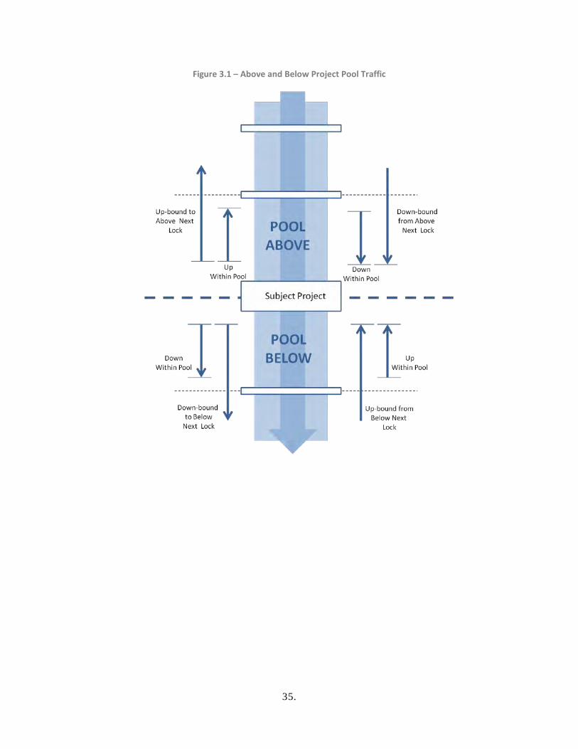
35.
Figure 3.1 – Above and Below Project Pool Traffic

36.
Estimating Closure Related Shipper Supply Chain Cost Burdens
At the core of this project is the analysis of the direct economic effects of unanticipated navigation lock closures using existing data and tools in ways that measurably reduce the resources required to undertake this research. Accomplishing this aim requires the execution of three primary task sets including:
■ Lock selection and data preparation; ■ Scenario design and traffic diversion assessments; and ■ The calculation of shipper supply chain costs before and after an unanticipated lock
closure.
This work is designed to conform to the P&G that currently guide the analysis of all federal inland navigation USACE infrastructure projects.17
4.1 LOCK SELECTION, TRAFFIC SAMPLES, AND DATA PREPARATION Section 3 describes the development and application of the screening tool used to identify four locks for inclusion in the current study. These locks included:
■ Markland Locks & Dam on the Mid-Ohio, near Cincinnati; ■ Calcasieu Lock on the Gulf Intracoastal Waterway, near Lake Charles, Louisiana; ■ LaGrange Lock & Dam, the lowest of the navigation locks on the Illinois River; and ■ Lock & Dam 25, north of St. Louis, near the Mississippi’s confluence with the Illinois
River.
The following process steps require the preparation of the navigation traffic data and other data resources necessary to identify and measure the effects of an unanticipated lock closure.
Sampling Lock Traffic When the volume of annual traffic through a subject lock is sufficiently small, it is sometimes possible to work with the entire population of annual traffic movements. However, in most cases, to do so is not feasible. Consequently, it is necessary to sample the annual traffic in a way that yields a manageable number of observations that can subsequently be used to accurately estimate population-wide impacts. This study used a stratified sample based on commodity groupings and the reported two-digit WCSC tonnages (described in Section 3.1). This sampling
17 See Economic and Environmental Principles and Guidelines for Water and Related Land Resources Implementation Studies, Washington, DC, March 10, 1983.
4

37.
pattern resulted in samples of between 900 and 1,400 records for each lock, representing 2-3 percent of all records and 10-12 percent of total 2014 tonnages.18
For each of the four subject locks, the result was a base sample dataset that included the data fields summarized in Table 4.1. Subsequent steps within the calculation of various supply chain cost components add many additional fields, but the initial WCSC record remains as the primary unit of observation throughout the analysis.
4.2 CLOSURE SCENARIOS, SHIPPER ALTERNATIVES, AND TRAFFIC DIVERSIONS
From a computation standpoint, the manipulation of the WCSC records is the most difficult task. However, in terms of analytical requirements, it is the identification of shipper alternatives and traffic diversions that poses the greatest challenge. Ultimately, meeting this challenge requires a variety of different approaches as described below.
When shippers encounter an unplanned lock outage, they are immediately faced with difficult questions. Some of these include:
■ Does the disruption affect more than one lock and does it affect system operations?
■ Is there available and reliable information about the probable closure duration?
■ Is some portion of the waterway still useful and, if so, can the usual carrier(s) continue to provide service over open waterway segments?
■ How large are existing user commodity inventories and how long will these last?
■ What are the costs, characteristics, and availabilities of transportation alternatives?
■ What are the potential penalties for delayed commodity delivery?
■ Are rivals similarly affected and how will they respond?
Depending on the answers to these questions, each shipper is likely to exhibit a variety of behaviors over time. Those with the luxury to do so may, in the short-run, cease shipping and rely on existing inventories. If that is not possible, but the duration is expected to be brief, some shippers may opt for relatively expensive stop-gap, short-run measures. Ultimately, however, if the unplanned outage is sufficiently long or if there is uncertainty about its duration, all affected shippers will be forced toward long-run strategies. These may involve re-sourcing inputs elsewhere, abandoning certain downstream markets, capital expenditures for new non-water freight transport facilities, or even shutting down a facility (i.e., worst case scenario). This sequence is depicted graphically in Figure 4.1.
18 In the late 1990s, study team members participated in a numerous USACE studies that experimented with a variety of different sampling methods. Then, as now, it appears that sampling techniques have little influence on analytical results.

38.
Figure 4.1 – Shipper Responses to Unplanned Lock Closures
To capture these various shipper responses under uncertainty, past studies typically have relied heavily on shipper surveys that pose questions based on possible outage durations of between 15 and 180 days. Shippers are asked to outline their responses under each scenario. While the aim of this complex survey structure is important, it can also lead to considerable confusion, an equal amount of speculation, and poor survey response rates.
Ideally, the perfect study would evaluate every alternative available to every affected shipper, then let the least-cost alternative identify the diversion. Unfortunately, this is impractical. Comparative alternative costs were calculated to identify diversions when no other information was available. However, where at all possible, this analysis relied on information from six other sources to identify the most likely long-run shipper diversions. These are bulleted then discussed individually. Information included:
■ Available Modal Alternatives
■ Shipment Characteristics
■ Ancillary Costs
■ Railroad Pricing Practices and Rate Data
■ Geographic Substitutes
■ Shipper Surveys and Interviews
Available Modal Alternatives Generally, it was assumed that highway access is ubiquitous. However, this is not the case for rail. In most cases, it was possible to identify whether or not shippers have existing railroad access and again, in most cases, the rail capacity that shipper access affords. The P & G that guide USACE studies suggest that new modal access can be added as necessary to create shipping alternatives.

39.
Shipment Characteristics Simple modal access does not necessarily guarantee that a modal alternative is viable. In some cases, shipment characteristics preclude an alternative even when that alternative is physically possible. For example, in our consideration of unscheduled outages at LaGrange or Lock and Dam 25 , all affected grain shippers are served by truck as are alternative port locations on waterways that would be unaffected by the outage. However, both LaGrange and L&D 25 accommodate approximately 10 million tons of corn and soybeans each year. Thus, while the economies evidenced by a limited number of longer truck movements suggest that trucking to alternative waterway locations might be a viable option, doing so for the whole of the diverted barge shipments would involve an additional 500,000 loaded truck trips per year and an additional 150 million truck miles in the affected states, an untenable solution.
Ancillary Costs As noted above, ancillary costs can be an important factor in shippers’ supply chain decision-making. Accordingly, even when comparative line-haul rates suggest that a modal alternative is viable, requisite changes in loading, unloading, or storage costs make the alternative untenable.
Railroad Pricing Practices and Rail Data Section 2.4 provides an extensive discussion of railroad issues and their effect on navigation project evaluations. In some settings, railroads have exercised the ability to influence traffic diversions through rate-setting. In the extreme, our analysis included this reality in the determination of least-cost alternatives.
Geographic Substitutes For some waterway traffic, origins and/or destinations are unchangeable. In other cases, specific products can be sourced from multiple locations that provide multiple transportation alternatives to shippers who might be affected by an unplanned lock outage. For example, some fertilizer components can be shipped to the upper Mississippi and Illinois basins from a variety of locations that involve multiple carriers across differing freight modes. Where this sort of geographic substitution is possible, it was included in our treatment of potential diversions.
Shipper Surveys and Interviews The study team developed a simple shipper survey and enlisted members of the National Waterways Foundation Study Oversight Team to distribute to shippers with traffic through Markland Locks. Unfortunately, the response rate was low and for this reason were not judged to be analytically useful. Fortunately, field notes from earlier studies existed. While these earlier interview results did not apply specifically to this study’s population of shippers, it was possible to identify patterns applicable to specific industries or commodities without regard to shipper specifics.
4.3 ESTIMATING TRANSPORTATION COSTS FOR EACH ALTERNATIVE This analysis compares economic outcomes under differing scenarios. In a freight setting, meeting this need generally requires a comparison of shipper costs with and without a proposed

40.
project or a proposed policy. The most essential the most essential tools are those used to estimate modal line-haul and terminal costs. In addition to the data elements described in Section 3.1, the current analysis relied on three such tools. These included:
■ A Barge Costing Model (BCM) developed by the Tennessee Valley Authority and certified for USACE applications;
■ Elements of STB’s Uniform Rail Costing System (URCS) cost estimates for CWS movements, along with supplemental information needed to produce railroad rate estimates; and
■ A motor carrier costing model made available through the American Transportation Research Institute (ATRI).
The Barge Costing Model (BCM) The BCM is a deterministic waterway costing model originally developed by the Tennessee Valley Authority, but now formally approved for use by the USACE. Figure 4.2 depicts the BCM operation.
Figure 4.2 – Barge Costing Model
The model is most easily executed on a movement-by-movement basis. However, it also features a batch mode for the manipulation of multiple records. In either case, the basic inputs can be drawn from individual WCSC records and include origin dock, destination dock, tonnage, commodity, etc. Prescribing a specific barge type or dimensions can be done, users can allow the routine to select an appropriate barge based on tonnage and commodity. Users can also modify various parameters such as fuel price, empty-return ratios, carrier rates of return, and in some cases, shipment routings.
41.
In addition to user supplied parameters, the model is updated periodically by the USACE to reflect changes in vessel horsepower, average vessel dimensions, average fuel costs, lock processing times, labor rates, etc. These parameters can also be manipulated by users, but only by those who are willing to explore the routine in areas beyond the typical user interface.
Railroad Movement Costing Given the economics and often limited competition that governs rail carriage, there is often a significant difference between estimated line-haul costs and observed railroad rates. Nonetheless, estimating incremental (or variable) costs, at least, provides a useful starting point for a more careful analysis of actual railroad rates.
Third-party logistics providers offer rail cost estimation software that functions much like the BCM described above. However, for those wishing to forego the expense of proprietary software, the CWS provides movement-specific cost estimates of variable costs based on the STB’s Uniform Rail Costing System (URCS). URCS has been routinely assailed by academic economists.19 Still, its use is mandated by the STB and its results govern the outcomes of regulatory proceedings, so that it is rarely successfully challenged.
Whether based on URCS or a proprietary product, any final rate estimates must scale variable costs so that the final rate estimates provide contributions toward the recovery of the fixed and common costs associated with network elements, as well as a competitive return on investment for rail carriers. In practice, railroads accomplish this by setting rates that reflect costs and the demand characteristics of rail shippers. Analysts can use observable shipment characteristics such as shipment size, distance, the number of competing railroads, the availability of modal substitutes, etc. as proxies for these demand characteristics.
Within the current analysis, URCS-based cost estimates were used and railroad rates for shipments with varying characteristics. The estimated rates and corresponding movements were submitted to third-party logistics providers who specialize in the subject commodities. Based on their feedback and insights, additional adjustments were made to obtain the rates used to reflect railroad costs.
Motor Carrier Costs As confounding as rail rates may be, truck rates are relatively simple to estimate. Because motor carriers face minimal fixed and virtually no common costs, and because motor carriage competition is, in most cases, intense, truck rates tend to closely follow operating costs.
In reality, it would be possible to independently assemble information describing motor carrier capital costs, vehicle maintenance costs, labor costs, fuel use, and administrative costs to generate an acceptable estimate of motor carrier costs that does not rely on any underlying model. However, in the current setting, this work is based on a motor carrier cost model
19 For example, see Wesley Wilson and Frank Wolak in Modernizing Freight Rail Regulation, Transportation Research Board Special Report 318, June 2015. Available at: http://www.trb.org/Publications/Blurbs/172736.aspx

42.
developed by ATRI.20 With the ATRI model as a benchmark, commodity-specific information developed by the Minnesota Department of Transportation to simulate commodity-based rate variability was used. The resulting motor carrier cost parameters are summarized in Table 4.1.
Table 4.1 – Motor Carrier Costs (Per Mile)
Total Truck Cost per Mile Commodity Grouping Single Driver Team Drivers
Overall $2.09 $2.71 Rubbish $4.67 $6.06 Dairy $3.12 $4.05 Food Products $2.73 $3.54 Paper $2.58 $3.34 Petroleum $2.46 $3.19 Timber $2.30 $2.99 Aggregate $2.12 $2.75 Industrial Supplies $2.06 $2.67 Construction $2.03 $2.63 Ag Chemicals $1.88 $2.44 Agricultural $1.85 $2.40 General Products $1.82 $2.36 Beverages $1.52 $1.97
Ancillary Supply Chain Costs As transportation professionals, we tend to focus on the line-haul, fleeting, and switching activities that we’re familiar with, but transportation decision-makers (shippers) are more inclined to focus on total supply chain costs when evaluating their choices. Therefore, it is important to represent these ancillary supply chain costs as accurately as possible when assessing a navigation project’s value.
Ancillary costs include outlays necessary for loading, unloading, commodity storage, loss and damage, safety stocks, and administrative expenses. In some cases, these costs are invariant to decisions regarding line-haul mode, but in other cases, mode choice has significant impacts on the magnitude of ancillary costs. Since there are presently no readily available data sets describing these ancillary costs, other sources were relied upon, including past studies, shipper queries, and industry publications.21
20 ATRI is a research organization supported directly by the American Trucking Association, See: An Analysis of the Operational Cost of Trucking: 2016 Update, September 2016. Available at: http://atri-online.org/wp-content/uploads/2016/10/ATRI-Operational-Costs-of-Trucking-2016-09-2016.pdf 21 The USACE’s Planning Center of Expertise for Inland Navigation (PCXIN) has developed an ancillary cost model that is scheduled for external review during the fall of 2017 and which will hopefully be made publicly available soon afterward.

43.
4.4 ESTIMATING THE SHIPPER SUPPLY CHAIN COST BURDEN Calculating averted shipper costs involves combining the data and tools with the diversion considerations described above to estimate both existing supply chain costs and the costs that would be incurred under the alternative scenario(s).
Table 4.2 illustrates a small portion of the summary spreadsheet developed as a part of the Markland analysis. The selected cells depict the rate calculations for several coal movements. Because of uncertainty regarding the most likely diversion, some movements required the calculation of supply chain costs under both all-rail and a combined, barge-rail alternative. Note also, that, while not used for the coal movements, the spreadsheet allows for the calculation of an all-truck alternative. Where the combined barge-rail alternative is tenable, it in fact, yields the lower alternative supply chain cost.
The estimation results yield Shipper Supply Chain Cost Burden – the increased supply chain costs associated with loss of the navigation alternative through the particular lock in dollars-per-ton. This value, multiplied by the tonnage yields an estimate total cost burden for the subject shipment. It is also often useful to use shipment distances to calculate both rates and averted shipper costs on a per-ton-mile-basis to be sure that the traditional distance-rate relationship is evident in the estimated rates. Finally, there may be instances in which the estimated averted costs are negative. On its face, this suggests either irrational behavior on the part of shippers or an error in the calculation of supply chain costs. Certainly, either of these is possible. However, there are also more reasonable explanations. Individual shippers may not immediately react to changing conditions. This is particularly true when there are significant costs to switching from one modal alternative to another. In fact, if these switching costs are sufficiently high, perfectly rational, profit-maximizing shippers may opt to suffer losses rather than switch at all if they view those losses to be tied to transient market conditions (say, for example, low water).
If conditions allow and the number of annual movement is not overwhelming, it is possible to estimate averted costs for the entire population of traffic using a subject lock. In such cases, the work of estimating supply chain cost differentials is finished. If, however, as in this work, the number of records is large so that movements are sampled, it is necessary to expand the averted shipper costs estimated for sample movements to the entire traffic population.
In the four cases treated here, the expansion of the sample findings was accomplished through the estimation of simple quadratic regression equations, where averted shipper costs served as the dependent variable and shipment distance and distance squared formed the independent variables. In those instances where the quadratic term failed to attain statistical significance, a simple linear form was used in place of the quadratic.

44.
Table 4.2 – Sample of Calculated Averted Supply Chain Costs
45.
Estimating Regional Economic Development Impacts
5.1 THE DIFFERENCE BETWEEN BENEFITS AND IMPACTS Discussions of public sector investments in transportation infrastructure involve a variety of economic concepts and terminology, including references to economic benefits and economic impacts. While functionally related, benefits and impacts are distinct concepts and their measures play
decidedly different roles in the decision-making process.
Investments in transportation infrastructure are undertaken because they improve economic outcomes – they either provide additional capacity that can accommodate more economic total activity or they relieve congestion and, thereby, avoid increasing transportation costs. Either way, there is a net improvement in aggregate welfare measured across the whole of the jurisdiction. In cases of federal investments, this implies that a subject investment provides net benefits to the nation as a whole. As specified in the P&G, these gains are referred to as National Economic Development (NED) benefits.22
Projects that improve economic efficiency usually attract economic activities from other regions. This attraction is a predicable response to the efficiency-enhancing investment, but rarely does it further increase the overall national benefits attributable to that investment. Instead, regional impacts represent a movement of economic activity in response to attainable efficiencies. Therefore, while these regional impacts may be important, they do not usually affect the national decision-making process. The P&G refer to these interregional transfers as Regional Economic Development (RED) benefits.23 Federal-level decision-makers rarely compute these RED benefits. Instead, if they are estimated, it is usually by regional-level stakeholders who wish to explore the regional benefits associated with national-level investments. It is just this sort of regional impact analysis that provides the results described in Section 2.3.
5.2 THE GENERAL STRUCTURE OF REGIONAL MODELS Typically, regional impact analyses are conducted in settings similar to the one depicted in Figure 5.1. A direct, exogenously imposed stimulus begins an iterative series of economic activities within a region. To begin with, those affected by the stimulus will often need to acquire additional goods and services from other sellers within the subject region. These are the Indirect Effects noted in the figure. Moreover, this iterative set of impacts changes incomes within the region which, in turn, leads to further changes in the magnitude of regional activity. These are represented by the Induced Effects depicted in Figure 5.2. These economic impacts are revealed
22 National Economic Development (NED) benefits are discussed throughout the P&G. However, the account definition is provided in Chapter 1 (1.7.1). Measurement issues are discussed in Chapter 2. 23 Regional Economic Development (RED) benefits are defined in Chapter 1 (1.7.4).
5
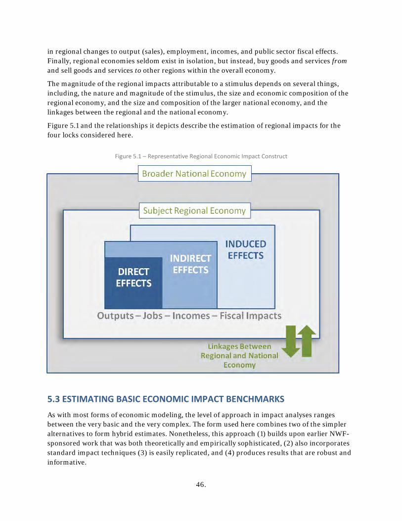
46.
in regional changes to output (sales), employment, incomes, and public sector fiscal effects. Finally, regional economies seldom exist in isolation, but instead, buy goods and services from and sell goods and services to other regions within the overall economy.
The magnitude of the regional impacts attributable to a stimulus depends on several things, including, the nature and magnitude of the stimulus, the size and economic composition of the regional economy, and the size and composition of the larger national economy, and the linkages between the regional and the national economy.
Figure 5.1 and the relationships it depicts describe the estimation of regional impacts for the four locks considered here.
Figure 5.1 – Representative Regional Economic Impact Construct
5.3 ESTIMATING BASIC ECONOMIC IMPACT BENCHMARKS As with most forms of economic modeling, the level of approach in impact analyses ranges between the very basic and the very complex. The form used here combines two of the simpler alternatives to form hybrid estimates. Nonetheless, this approach (1) builds upon earlier NWF-sponsored work that was both theoretically and empirically sophisticated, (2) also incorporates standard impact techniques (3) is easily replicated, and (4) produces results that are robust and informative.

47.
Economic Form of Direct Effects The stimulus or Direct Effect depicted in Figure 5.1 can come in one of two forms. It can be a demand-side stimulus, where their exogenous force increase or decrease demands for goods or services produced in the subject region or the stimulus can be a supply shock, where there is an exogenous change in the cost of producing goods or services within the region. Changes in the availability or performance of transportation infrastructures are almost always among this latter group. Specifically, in this study, the stimulus (or shock) is the substantial increase in transportation cost that is predicted under an unscheduled lock closure. This form of stimulus is identical in nature to the overall system outage that was the basis for the 2014 NWF-sponsored study: Inland Navigation in the United States: An Evaluation of Economic Impacts and the Potential Effects on Infrastructure Investment.
Geography of Direct Effects and Consequent Impacts The increased transportation costs attributable to a lock closure are tied to the locations of the producers who originate waterborne shipments and the subsequent users of the shipped commodities, not the location of the lock itself. In this analysis, the initial river origin and final river destination are used as proxies for the geographical distribution of impacts. In addition, the analysis estimates with one exception, that the increased cost of transportation owing to a lock outage would be split evenly between the waterway origin and destination locations. In the case of farm products, the stimulus (increased costs) is placed exclusively at the origin, reflecting that most are export shipments
There are two reasons for the asymmetric treatment of farm products, particularly in the current application. First, the vast majority of down-bound grain transiting LaGrange and L&D 25 is bound for export over the Louisiana Gulf. Thus, these shipments generate relatively little economic activity at their domestic destinations. As importantly, there is a widely held conclusion that level of corn and soybean production in the Illinois and upper Mississippi basins is unlikely to be impacted by increased transportation costs and that changes in the export availability of these goods would not affect final market prices in the global markets where they compete. This implies that basin producers would likely absorb the majority of transportation cost increases in the form of lost incomes.
Determination and Effects of Study Regions The extent of region or regions in which economic impacts are evaluated can be varied based on the purpose of the analysis and the availability of data. However, the scale of subject regions does affect the magnitude of the estimated effects. Referring again to Figure 5.1, there are linkages between the study region and the world beyond. Among other things, these linkages include leakages of economic consequences from the study region into the broader economy. The extent of these leakages depends on the extent to which regional demands can be satisfied internally. This, in turn, usually depends on the size of the study region. As a rule, larger regions are better able to self-supply economic resources, so that impacts are generally greater than would be generated by a similar shock in a geographically smaller region.
Figure 5.2 depicts the study regions used in the NWF’s 2014 work. In the current application, the earlier empirical results are used to generate state-level predictions. On its face, this

48.
application may seem tenuous. However, the study team judged that use of the 2014 results is, in fact, appropriate. Specifically, the amount of economic activity and resources available in any of the affected states is roughly analogous to the total economic activity evidence in the study region where that state is located. Moreover, the economic characteristics within a specific state tend to mirror those observed within the larger region.
Figure 5.2 – 2014 Study Region Geography
Current Study Impact Benchmark Estimation For a variety of reasons, the methodology outlined above yields what may be interpreted as upper boundaries for output, income, and employment effects. Consequently, earlier reviewers of the current study suggested that these upper bound estimates be accompanied by corresponding estimates of what are likely to be lower boundaries for the same estimated outcomes. Following this suggestion, the study team produced high and low impact estimates for each affected state. It is the midpoint or average of these estimates that are reported in Section 2.
Upper-Bound Estimates Within the current study, the Direct Effects depicted in Figure 5.1 are the avoided increases in supply chain costs that would result from an unscheduled lock outage. Their analogue in the 2014 study is the increase in system-wide user costs that would occur from

49.
a full system outage. Given this ready comparison it was relatively easy to derive transportation cost based multipliers and apply them to current study cost projections. Specifically, for each multiplier i, multipliers are calculated as:
MULTi = IMPACT14i COST14i
Based on this construct, the multipliers applied here are provided in Table 5.1.24
Table 5.1 – Study-Derived Economic Impact Multipliers
(Based Against Navigation-Related Avoided Costs)
State
Output Multiplier per $1 of Avoided
Cost
Income Multiplier per $1 of Avoided Cost
Employment Multiplier per $10 Million of Avoided Cost
AL 5.125 1.229 18.3300 AR 5.549 1.793 22.5400 FL 7.597 1.767 22.7500 IA 5.549 1.793 22.5400 IL 4.101 1.242 18.2200 IN 2.654 0.691 13.9000 KY 2.654 0.691 13.9000 LA 5.718 1.326 18.6400
MN 5.549 1.793 22.5400 MO 5.549 1.793 22.5400 MS 3.246 0.788 14.2100 OH 2.654 0.691 13.9000 OK 3.839 0.885 14.5200 PA 2.654 0.691 13.9000 TN 2.654 0.691 13.9000 TX 5.718 1.767 22.7500 WI 5.549 1.793 22.5400 WV 2.654 0.691 13.9000
Lower-Bound Estimates There are numerous alternatives to the methodology described above. To estimate the lower bound of potential economic impacts, the study team applied multipliers made available by the U.S. Bureau of Economic Analysis as part of its RIMS II Regional Input-Output Modeling System.25
24 Some states are served by waterway segments that lie in more than one of the 2014 regions. In these cases, the multipliers were calculated as the simple mean of the corresponding regional average. 25 For a full description of the RIMS II economic simulation products and their use see: RIMS II, An Essential Tool for Regional Developers and Planners, available at: https://www.bea.gov/regional/pdf/rims/RIMSII_User_Guide.pdf

50.
Like most input-out packages, the RIMS II products are easily applied to simulate demand-side stimuli, but are more difficult to use in the case of a supply-side disturbance as is modeled here. Typically, in such cases, supply-side shocks are treated as overall changes to regional incomes. This tends to understate the magnitude of impacts or, as was desired here, produce a lower bound on probable output, income, and employment impacts. The correspond RIMS II multipliers are reproduced here in Table 5.2.
Finally, it is the average or blended results from these alternative methods that are reported in Section 2, Tables 2.6 – 2.9.
Table 5.2 – RIMS II Impact Multipliers (Household Incomes) (Based On Navigation-Related Avoided Costs)
State
Output Multiplier per $1 of Avoided
Cost
Income Multiplier per $1 of Avoided
Cost
Employment Multiplier per $10 Million of Avoided Cost
AL 1.0728 0.3250 10.0086 AR 0.9482 0.2884 8.5720 FL 1.2510 0.3876 11.6335 IA 0.9447 0.2848 8.6470 IL 1.4083 0.4085 9.7650 IN 1.1960 0.3504 9.5203 KY 1.0862 0.3107 9.0880 LA 1.0339 0.3238 9.3414
MN 1.3021 0.3792 9.8312 MO 1.2427 0.3491 9.9061 MS 0.9858 0.2950 9.3012 OH 1.2929 0.3829 10.8242 OK 1.1125 0.3408 9.6592 PA 1.2694 0.3691 9.4631 TN 1.3523 0.3950 10.3448 TX 1.4871 0.4427 11.1339 WI 1.0724 0.3338 9.3603 WV 0.8512 0.2496 7.8008

51.
Final Thoughts The objective of this analysis was to develop detailed information cataloguing the economic effects of unplanned lock outages at four locations. However, a second important goal was to demonstrate that primary and secondary data can be combined with existing (or slightly modified) modeling platforms to estimate these navigation outcomes with less extensive, expensive, and time-consuming field work.
Within the course of this work, the study team developed two new metrics for measuring the nature and extent of inland navigation’s commercial influence. These include the Corridor Concentration Metric presented in Section 2 and further described in Appendix 1 and the Above and Below Pool traffic measures described in Sections 2 and 3.
Both measures provide easily calculable metrics that capture important aspects of commercial navigation. Both the corridor concentration metric and the above and below pool tonnage measures emerged in response to specific sponsor questions and both have potentially important implications in the future evaluation of inland navigation investments. Accordingly, we would strongly urge others to further develop both the calculation and use of these metrics and to explore additional ways to quantitatively address relevant system use and performance.
Finally, the study’s results confirm many long-held beliefs, but also offer new insights. A few (though not all) key findings are summarized in the Executive Summary. These are repeated here for emphasis and with the hope that readers will find it useful to carry these results forward in other uses. It is clear, to the study team at least, that the nation’s navigable waterways represent an important linkage that is essential in its long-run value to both domestic commerce and global trade. We hope this is a message that will be communicated effectively going forward.
6
A FEW KEY FINDINGS
■ Each of the four locks considered within the study helps shippers to avoid more than $1 Billion in additional transportation costs each year.
■ The important roles played by individual navigation projects span a broad range of both geographies and economic purposes, and in some cases provide freight mobility that could not be easily replaced by other transport modes.
■ While every state that originates or terminates traffic supported by the four locks benefits from inland navigation’s availability, the results reflect the waterway’s extraordinary commercial value to Louisiana, Texas, and Illinois.
■ In the cases of LaGrange Lock & Dam and Lock & Dam 25, trucking to alternative waterway locations would mean an additional 500,000 loaded truck trips per year and an additional 150 million truck miles in the affected states. This is not tenable.
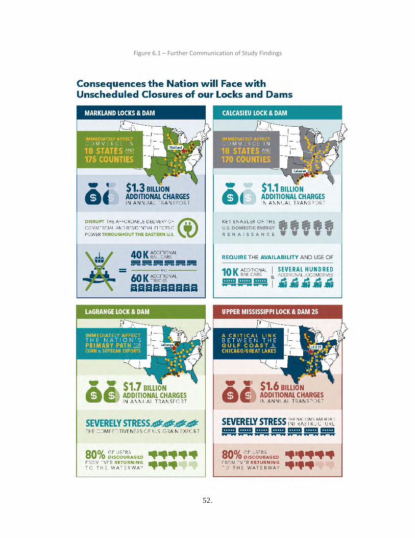
52.
Figure 6.1 – Further Communication of Study Findings
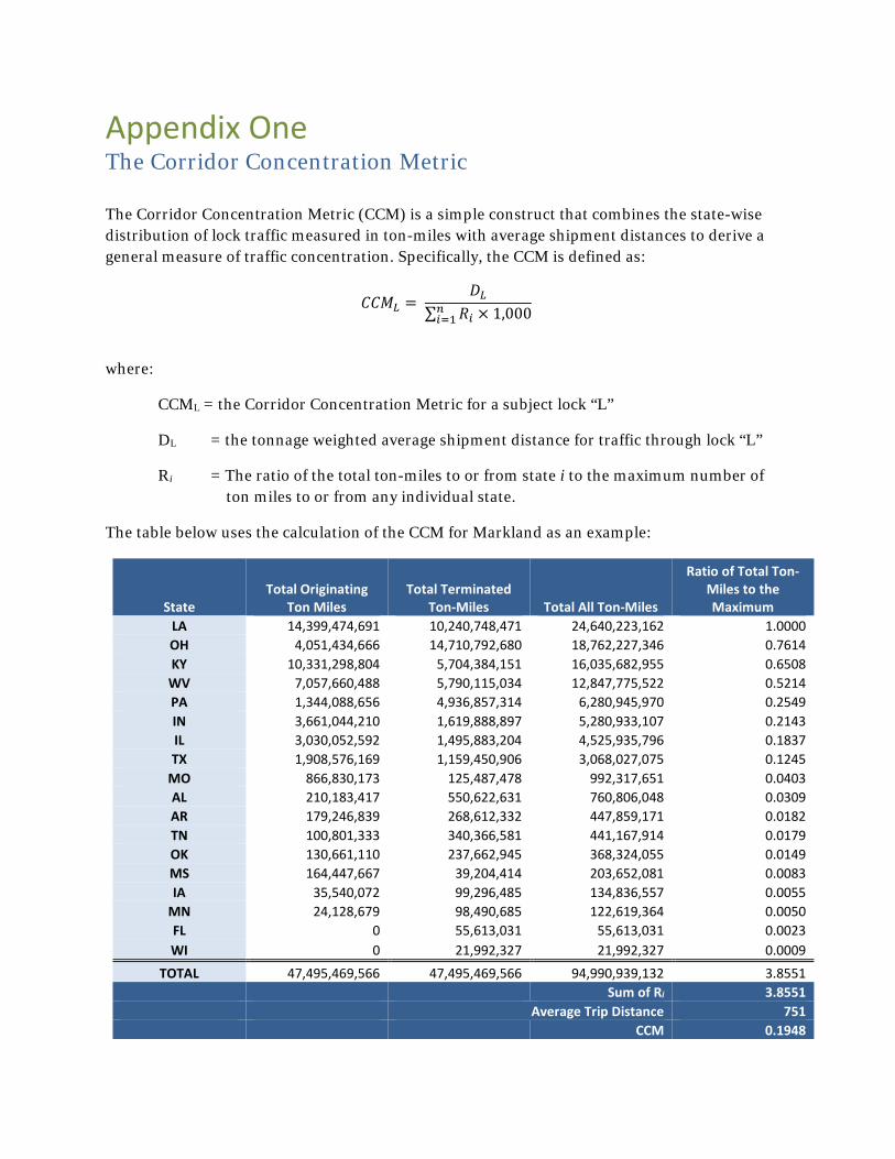
53.
Appendix One The Corridor Concentration Metric
The Corridor Concentration Metric (CCM) is a simple construct that combines the state-wise distribution of lock traffic measured in ton-miles with average shipment distances to derive a general measure of traffic concentration. Specifically, the CCM is defined as:
𝐶𝐶𝐶𝐶𝐶𝐶𝐿𝐿 = 𝐷𝐷𝐿𝐿
∑ 𝑅𝑅𝑖𝑖𝑛𝑛𝑖𝑖=1 × 1,000
where:
CCML = the Corridor Concentration Metric for a subject lock “L”
DL = the tonnage weighted average shipment distance for traffic through lock “L”
Ri = The ratio of the total ton-miles to or from state i to the maximum number of ton miles to or from any individual state.
The table below uses the calculation of the CCM for Markland as an example:
State Total Originating
Ton Miles Total Terminated
Ton-Miles Total All Ton-Miles
Ratio of Total Ton-Miles to the Maximum
LA 14,399,474,691 10,240,748,471 24,640,223,162 1.0000 OH 4,051,434,666 14,710,792,680 18,762,227,346 0.7614 KY 10,331,298,804 5,704,384,151 16,035,682,955 0.6508 WV 7,057,660,488 5,790,115,034 12,847,775,522 0.5214 PA 1,344,088,656 4,936,857,314 6,280,945,970 0.2549 IN 3,661,044,210 1,619,888,897 5,280,933,107 0.2143 IL 3,030,052,592 1,495,883,204 4,525,935,796 0.1837 TX 1,908,576,169 1,159,450,906 3,068,027,075 0.1245
MO 866,830,173 125,487,478 992,317,651 0.0403 AL 210,183,417 550,622,631 760,806,048 0.0309 AR 179,246,839 268,612,332 447,859,171 0.0182 TN 100,801,333 340,366,581 441,167,914 0.0179 OK 130,661,110 237,662,945 368,324,055 0.0149 MS 164,447,667 39,204,414 203,652,081 0.0083 IA 35,540,072 99,296,485 134,836,557 0.0055
MN 24,128,679 98,490,685 122,619,364 0.0050 FL 0 55,613,031 55,613,031 0.0023 WI 0 21,992,327 21,992,327 0.0009
TOTAL 47,495,469,566 47,495,469,566 94,990,939,132 3.8551 Sum of Ri 3.8551 Average Trip Distance 751 CCM 0.1948

54.
Appendix Two Additional Screening Tool Results

No. Lock River
Year
Open Rehab Status
Num
Chambers Bank Lift
Chamber
Length
Chamber
Width Mooring State Vessels
1 Claiborne Alabama 1969 none operational 1 L 30 600 84 N AL 77
2 Millers Ferry Alabama 1969 none operational 1 L 45 600 84 N AL 114
3 Robert F. Henry Alabama 1972 none operational 1 L 45 600 84 N AL 62
4 Great Bridge Albemarle and Chesap 1932 none operational 1 L 3 600 72 N VA
5 L&D 2 Allegheny 1934 none operational 1 L 11 360 56 Y PA 5,501
6 L&D 3 Allegheny 1934 none operational 1 L 14 360 56 Y PA
7 L&D 4 Allegheny 1927 none operational 1 R 11 360 56 Y PA 1701
8 L&D 5 Allegheny 1927 none seasonal 1 R 12 360 56 N PA 1121
9 L&D 6 Allegheny 1928 none seasonal 1 R 12 360 56 N PA 377
10 L&D 7 Allegheny 1930 none seasonal 1 R 13 360 56 N PA 14
11 L&D 8 Allegheny 1931 none seasonal 1 L 18 360 56 N PA
12 L&D 9 Allegheny 1938 none seasonal 1 L 22 360 56 Y PA
13 Jim Woodruff Apalachicola 1954 none operational 1 R 33 450 82 N FL
14 Arthur V. Ormond Arkansas 1969 none operational 1 R 19 600 110 Y AR 875
15 Col Charles D. Maynard Arkansas 1968 none operational 1 L 17 600 110 Y AR 1499
16 Dardanelle Arkansas 1969 none operational 1 L 55 600 110 Y AR 898
17 David D. Terry Arkansas 1968 none operational 1 L 18 600 110 Y AR 1250
18 Emmet Sanders Arkansas 1968 none operational 1 R 14 600 110 Y AR 1402
19 James W. Trimble Arkansas 1969 none operational 1 R 20 600 110 Y AR 2393
20 Joe Hardin Arkansas 1868 none operational 1 L 20 600 110 Y AR 1284
21 Murray Arkansas 1969 none operational 1 R 18 600 110 Y AR 1081
22 Norrell (Post Canal) Arkansas 1967 none operational 1 L 30 600 110 N AR 1280
23 Ozark - Jetta Taylor Arkansas 1969 none operational 1 L 34 600 110 Y AR 825
24 Robert S. Kerr Arkansas 1970 none operational 1 L 48 600 110 N OK 1246
25 Toad Suck Ferry Arkansas 1969 none operational 1 L 16 600 110 Y AR 878
26 W.D. Mayo Arkansas 1971 none operational 1 R 21 600 110 N OK 1196
27 Webers falls Arkansas 1970 none operational 1 L 30 600 110 N OK 1429
28 WILBUR D MILLS Arkansas 1967 none operational 1 L 20 600 110 N AR 1350
29 Berwick Atchafalaya 1950 none operational 1 R 14 307 45 N LA 3509
30 Jonesville Black 1972 none operational 1 R 30 600 84 N LA 998
31 Black Rock Black Rock Canal 1914 none operational 1 R 5 650 70 N NY 2069
32 Armistead I. Selden Black Warrior 1957 none operational 1 L 28 600 110 N WA 1508
33 Hohn Hollis Bankhead Black Warrior 1975 none operational 1 L 22 600 110 N AL 1193
34 Holt Black Warrior 1966 none operational 1 L 64 600 110 N AL 1458
35 William Bacon Oliver Black Warrior 1991 none operational 1 L 68 600 110 N AL 1341
36 Calcasieu Calcasieu River 1968 none operational 1 L 0 575 56 N LA 13247
37 Moore Haven Caloosahtchee 1953 none operational 1 R 2 250 50 Y FL 4281
38 W. P. Franklin Caloosahtchee 1965 none operational 1 L 3 400 56 Y FL 7411
39 Thomas J. Obrien Calumet 1960 none operational 1 R 4 1000 110 Y IL 10444
40 1 Cape Fear 1915 none operational 1 R 11 200 40 Y NC
41 2 Cape Fear 1917 none operational 1 R 9 200 40 Y NC
42 William O. Huske Cape Fear 1935 none operational 1 R 9 300 40 Y NC
43 George W. Andrews Chattahoochee 1962 none operational 1 L 25 450 82 N GA 208
44 Walter F. George Chattahoochee 1963 none operational 1 L 88 450 82 N GA 231
45 Chicago Chicago River 1938 none operational 1 R 4 600 80 N IL 34979

No. Lock River
Year
Open Rehab Status
Num
Chambers Bank Lift
Chamber
Length
Chamber
Width Mooring State Vessels
46 Melton Hill Clinch River 1963 none operational 1 R 58 400 75 N TN
47 Barkley Cumberland 1964 none operational 1 L 57 800 110 Y KY 1367
48 Cheatham Cumberland 1952 none operational 1 R 26 800 110 Y TN 2007
49 Cordell Hull Cumberland 1973 none replaced 1 L 59 400 84 N TN
50 Old Hickory Cumberland 1954 none operational 1 L 60 400 84 Y TN 2134
51 Deep Creek Dismal Swamp Canal 1940 none operational 1 L 12 300 52 N VA 1484
52 South Mills Dismal Swamp Canal 1941 none operational 1 L 12 300 52 N NC 1433
53 Freshwater Bayou Freshwater Bayou 1968 none operational 1 R 4 600 84 N LA 13511
54 Bayou Boeuf GIWW 1954 none operational 1 R 11 1156 75 N LA 18251
55 Calcasieu GIWW 1950 none operational 1 R 4 1205 75 N LA 14437
56 Leland Bowman GIWW 1985 none operational 1 R 5 1200 110 N LA 14401
57 Algiers GIWW Algiers Canal 1956 none operational 1 R 18 797 75 N LA 10915
58 Bayou Sorrel GIWW Morgan City Port Al. 1952 none operational 1 R 21 800 56 N LA 7108
59 Port Allen GIWW Morgan City Port Al. 1961 none operational 1 R 45 1202 84 N LA 7930
60 Brazos East GIWW Texas 1943 none operational 1 C 0 750 75 Y TX 27755
61 Brazos West GIWW Texas 1943 none operational 1 C 0 750 75 Y TX 25553
62 Colorado River East GIWW Texas 1944 none operational 1 L 12 1200 75 Y TX 22069
63 Colorado River West GIWW Texas 1944 none operational 1 L 12 1200 75 Y TX 22306
64 Harvey GIWW West 1935 none operational 1 R 20 425 75 N LA 6003
65 GREEN RIVER - 1 Green 1956 none operational 1 R 8 600 84 Y KY 3495
66 GREEN RIVER - 2 Green 1956 none operational 1 R 14 600 84 Y KY 1431
67 Inner Harbor Nav Canl Lk GWW East 1923 none operational 1 L 17 640 75 N LA 8500
68 Brandon road Illinois 1933 1988 operational 1 R 34 600 110 N IL 3446
69 Dresden island Illinois 1933 1995 operational 1 L 22 600 110 Y IL 3437
70 Lagrange Illinois 1939 1988 operational 1 R 10 600 110 N IL 3063
71 Lockport Illinois 1933 1989 operational 1 L 39 600 110 N IL 3342
72 Marseilles Illinois 1933 1996 operational 1 L 24 600 110 Y IL 3765
73 Peoria Illinois 1938 1990 operational 1 L 11 600 110 N IL 3316
74 Starved Rock Illinois 1933 1996 operational 1 R 19 600 110 Y IL 3886
75 London Kanawha 1933 none operational 2 R 24 360 56 N WV 935
76 Marmet Kanawha 2008 none operational 3 R 24 360 56 Y WV 2039
77 Winfield Kanawha 1997 none operational 3 R 28 360 56 Y WV 1624
78 Kaskaskia Kaskaskia 1973 none operational 1 R 29 600 84 N IL 1985
79 Catfish Point Mermentau 1951 none operational 1 R 0 500 56 N LA 1087
80 CHAINS OF ROCKS L/D 27 Mississippi 1953 2009 operational 2 L 21 1200 110 N IL 2343
81 LOCK & DAM 1 Mississippi 1930 1980 seasonal 2 R 38 400 56 Y MN 2358
82 LOCK & DAM 10 Mississippi 1936 2006 seasonal 1 R 8 600 110 N IA 3678
83 LOCK & DAM 11 Mississippi 1937 2012 operational 1 R 12 600 110 N IA 5010
84 LOCK & DAM 12 Mississippi 1939 2000 operational 1 R 9 600 110 Y IA 2831
85 LOCK & DAM 13 Mississippi 1938 1996 operational 1 L 11 600 110 Y IL 2387
86 LOCK & DAM 14 Mississippi 1922 1996 operational 2 R 11 600 110 N IA 2292
87 LOCK & DAM 15 Mississippi 1934 1993 operational 2 L 16 600 110 N IA 2539
88 LOCK & DAM 16 Mississippi 1937 1991 operational 1 L 9 600 110 N IL 2723
89 LOCK & DAM 17 Mississippi 1939 1988 operational 1 L 8 600 110 N IL 2108
90 LOCK & DAM 18 Mississippi 1937 1990 operational 1 L 10 600 110 Y IL 2424
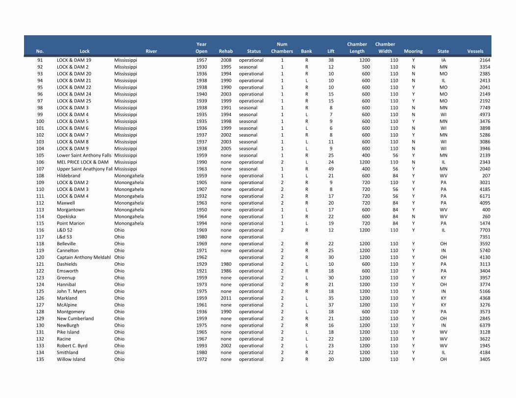
No. Lock River
Year
Open Rehab Status
Num
Chambers Bank Lift
Chamber
Length
Chamber
Width Mooring State Vessels
91 LOCK & DAM 19 Mississippi 1957 2008 operational 1 R 38 1200 110 Y IA 2164
92 LOCK & DAM 2 Mississippi 1930 1995 seasonal 1 R 12 500 110 N MN 3354
93 LOCK & DAM 20 Mississippi 1936 1994 operational 1 R 10 600 110 N MO 2385
94 LOCK & DAM 21 Mississippi 1938 1990 operational 1 L 10 600 110 N IL 2413
95 LOCK & DAM 22 Mississippi 1938 1990 operational 1 R 10 600 110 Y MO 2041
96 LOCK & DAM 24 Mississippi 1940 2003 operational 1 R 15 600 110 Y MO 2149
97 LOCK & DAM 25 Mississippi 1939 1999 operational 1 R 15 600 110 Y MO 2192
98 LOCK & DAM 3 Mississippi 1938 1991 seasonal 1 R 8 600 110 N MN 7749
99 LOCK & DAM 4 Mississippi 1935 1994 seasonal 1 L 7 600 110 N WI 4973
100 LOCK & DAM 5 Mississippi 1935 1998 seasonal 1 R 9 600 110 Y MN 3476
101 LOCK & DAM 6 Mississippi 1936 1999 seasonal 1 L 6 600 110 N WI 3898
102 LOCK & DAM 7 Mississippi 1937 2002 seasonal 1 R 8 600 110 Y MN 5286
103 LOCK & DAM 8 Mississippi 1937 2003 seasonal 1 L 11 600 110 N WI 3086
104 LOCK & DAM 9 Mississippi 1938 2005 seasonal 1 L 9 600 110 N WI 3946
105 Lower Saint Anthony Falls Mississippi 1959 none seasonal 1 R 25 400 56 Y MN 2139
106 MEL PRICE LOCK & DAM Mississippi 1990 none operational 2 L 24 1200 110 N IL 2343
107 Upper Saint Anathjony FallsMississippi 1963 none seasonal 1 R 49 400 56 Y MN 2040
108 Hildebrand Monongahela 1959 none operational 1 L 21 600 84 Y WV 207
109 LOCK & DAM 2 Monongahela 1905 none operational 2 R 9 720 110 Y PA 3021
110 LOCK & DAM 3 Monongahela 1907 none operational 2 R 8 720 56 Y PA 4185
111 LOCK & DAM 4 Monongahela 1932 none operational 2 R 17 720 56 Y PA 6171
112 Maxwell Monongahela 1963 none operational 2 R 20 720 84 Y PA 4095
113 Morgantown Monongahela 1950 none operational 1 L 17 600 84 Y WV 400
114 Opekiska Monongahela 1964 none operational 1 R 22 600 84 N WV 260
115 Point Marion Monongahela 1994 none operational 1 L 19 720 84 Y PA 1474
116 L&D 52 Ohio 1969 none operational 2 R 12 1200 110 Y IL 7703
117 L&d 53 Ohio 1980 none operational 7351
118 Belleville Ohio 1969 none operational 2 R 22 1200 110 Y OH 3592
119 Cannelton Ohio 1971 none operational 2 R 25 1200 110 Y IN 5740
120 Captain Anthony Meldahl Ohio 1962 operational 2 R 30 1200 110 Y OH 4130
121 Dashields Ohio 1929 1980 operational 2 L 10 600 110 Y PA 3113
122 Emsworth Ohio 1921 1986 operational 2 R 18 600 110 Y PA 3404
123 Greenup Ohio 1959 none operational 2 L 30 1200 110 Y KY 3957
124 Hannibal Ohio 1973 none operational 2 R 21 1200 110 Y OH 3774
125 John T. Myers Ohio 1975 none operational 2 R 18 1200 110 Y IN 5166
126 Markland Ohio 1959 2011 operational 2 L 35 1200 110 Y KY 4368
127 McAlpine Ohio 1961 none operational 2 L 37 1200 110 Y KY 3276
128 Montgomery Ohio 1936 1990 operational 2 L 18 600 110 Y PA 3573
129 New Cumberland Ohio 1959 none operational 2 R 21 1200 110 Y OH 2845
130 NewBurgh Ohio 1975 none operational 2 R 16 1200 110 Y IN 6379
131 Pike Island Ohio 1965 none operational 2 L 18 1200 110 Y WV 3128
132 Racine Ohio 1967 none operational 2 L 22 1200 110 Y WV 3622
133 Robert C. Byrd Ohio 1993 2002 operational 2 L 23 1200 110 Y WV 1945
134 Smithland Ohio 1980 none operational 2 R 22 1200 110 Y IL 4184
135 Willow Island Ohio 1972 none operational 2 R 20 1200 110 Y OH 3405
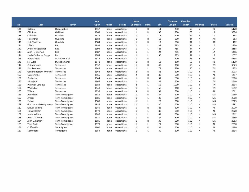
No. Lock River
Year
Open Rehab Status
Num
Chambers Bank Lift
Chamber
Length
Chamber
Width Mooring State Vessels
136 Ortona Okeechobee 1937 none operational 1 R 11 250 50 Y FL 5128
137 Old River Old River 1963 none operational 1 R 35 1200 75 N LA 3376
138 Columbia Ouachita 1972 none operational 1 L 18 600 84 N LA 393
139 Felsenthal Ouachita 1984 none operational 1 R 18 600 84 N AR 263
140 H.K. Thatcher Ouachita 1984 none operational 1 R 12 600 84 N AR 182
141 L&D 3 Red 1992 none operational 1 L 31 785 84 N LA 1330
142 Joe D. Waggonner Red 1994 none operational 1 L 25 785 84 N LA 2158
143 John H. Overton Red 1987 none operational 1 L 24 785 84 N LA 1416
144 Lindy Claiborne Boggs Red 1984 none operational 1 L 36 785 84 N LA 1657
145 Port Mayaca St. Lucie Canal 1977 none operational 1 R 2 400 56 Y FL 4394
146 St. Lucie St. Lucie Canal 1941 none operational 1 R 13 250 50 Y FL 5129
147 Chickamauga Tennessee 1937 none operational 1 R 49 360 60 Y TN 3623
148 Fort Loudoun Tennessee 1943 none operational 1 L 72 360 60 N TN 1453
149 General Joseph Wheeler Tennessee 1963 none operational 2 R 48 600 110 Y AL 2003
150 Guntersville Tennessee 1965 none operational 2 R 39 600 110 Y AL 1497
151 Kentucky Tennessee 1944 none operational 1 R 57 600 110 Y KY 2986
152 Nickajack Tennessee 1967 none operational 1 R 39 600 110 Y TN 1640
153 Pickwick Landing Tennessee 1984 none operational 2 L 55 1000 110 Y TN 2394
154 Watts Bar Tennessee 1941 none operational 1 L 58 360 60 Y TN 1592
155 Wilson Tennessee 1959 none operational 3 R 94 600 110 N AL 2661
156 Aberdeen Tenn-Tombigbee 1985 none operational 1 R 27 600 110 N MS 1969
157 Amory Tenn-Tombigbee 1985 none operational 1 L 30 600 110 N MS 2008
158 Fulton Tenn-Tombigbee 1985 none operational 1 L 25 600 110 N MS 2025
159 G.V. Sonny Montgomery Tenn-Tombigbee 1985 none operational 1 L 30 600 110 N MS 1991
160 Glover Wilkins Tenn-Tombigbee 1985 none operational 1 R 25 600 110 N AL 2020
161 Howell Heflin Tenn-Tombigbee 1978 none operational 1 L 36 600 110 N AL 2020
162 Jamie Whitten Tenn-Tombigbee 1985 none operational 1 L 84 600 110 N MS 2312
163 John C. Stennis Tenn-Tombigbee 1980 none operational 1 R 27 600 110 N MS 2289
164 John E. Rankin Tenn-Tombigbee 1985 none operational 1 R 30 600 110 N MS 2053
165 Tom Bevill Tenn-Tombigbee 1979 none operational 1 L 27 600 110 N AL 2090
166 Coffeeville Tombigbee 1960 none operational 1 R 34 600 110 N AL 2490
167 Demopolis Tombigbee 1954 none operational 1 L 40 600 110 N AL 2594

No.
1
2
3
4
5
6
7
8
9
10
11
12
13
14
15
16
17
18
19
20
21
22
23
24
25
26
27
28
29
30
31
32
33
34
35
36
37
38
39
40
41
42
43
44
45
Ktons Lockages WCSC Tons LPMS Tons WCSC Ton-Miles
System
Lockages
System
Lockages per
Barge
Above Pool
Tonnage Below Pool Tonnage Pool Above Total Pool Below Total
65 0 0 0 0
98 0 0 0 0
34 0 0 0 0
667896 941000 215389170 287 1 0 0 0 0
2148 3803 1732368 2148000 438768003 15628 10 0 0 0 0
1732368 2164000 438768003 15628 10 0 0 0 0
412 1117 294446 412000 173054654 2437 12.4 0 1,358,167 0 1,358,167
75 544 6593 75000 12183864 104 26 0 113,374 0 113,374
21 100 6593 21000 12183864 104 26 0 0 0 0
75 7.25 6593 14000 12183864 104 26 0 0 0 0
0 0 0 0
0 0 0 0
0 0 0 0
6759 1189 6865895 6759000 6300563711 74708 17.7 0 493,143 0 493,143
8638 1711 8829595 8638000 7622745294 83444 15.5 4,874 474,968 4,874 474,968
6723 1184 6807975 6723000 6252996277 74262 17.7 0 18,845 0 18,845
8441 1581 8834469 8441000 7622802803 83486 15.5 1,089,395 0 1,089,395 0
8800 1713 9312829 8800000 7879113329 84641 14.9 4,921 42,491 4,921 42,491
7303 2431 22227660 7303000 6414502087 73530 6.4 704,200 0 704,200 0
8756 1643 9355320 8756000 7901242586 84722 14.9 0 398,688 0 398,688
6851 1363 7173279 6851000 6357914368 75112 17.2 3,344 2,476,789 3,344 2,476,789
9105 1653 9760696 9105000 8106186465 85217 14.3 0 0 0 0
6137 1147 6690500 6137000 6198273127 73464 17.9 800,260 93,525 800,260 93,525
5794 1446 6247617 5794000 5839927519 69661 18.2 0 0 0 0
6789 1202 7176623 6789000 6357954334 75132 17.2 439,178 0 439,178 0
5793 1414 6247617 5793000 5839927519 69661 18.2 0 1,784,821 0 1,784,821
5416 1475 5908615 5416000 5571702408 66340 18.4 0 57,595 0 57,595
9140 1679 9760696 9140000 8106186465 85217 14.3 0 0 0 0
22 2939 27079187 22000 23529847909 143368 10.2 0 0 0 0
1076 1045 980457 310860181 1590 3.2 0 0 0 0
82 1532 82000 0 0 0 0
7693 1413 7496716 7693000 3094603079 31318 6.9 633,806 4,768,059 633,806 4,768,059
4505 1034 5776575 5941000 2181969077 25613 6.7 18,000 687,550 2,249,033 1,408,901
5941 1221 4385674 4505000 1681101232 20935 7.2 2,249,033 1,408,901 18,000 687,550
7071 1268 6748538 7071000 2479373640 28501 6.5 264,900 422,856 264,900 422,856
469 3987 6875951 469000 2330362699 14708 4.4 153,786 53,103,923 153,786 53,103,923
4 3511 1500 4000 216000 15 5 0 0 0 0
4 5598 1500 4000 216000 15 5 0 0 0 0
5916 4279 5742072 5916000 6164914723 39822 11 0 0 0 0
0 0 0 0
0 0 0 0
0 0 0 0
117 6 0 0 0 0
117 0 0 0 0
245 10959 5742072 245000 6164914723 39822 11 0 0 0 0

No.
146
47
48
49
50
51
52
53
54
55
56
57
58
59
60
61
62
63
64
65
66
67
68
69
70
71
72
73
74
75
76
77
78
79
80
81
82
83
84
85
86
87
88
89
90
Ktons Lockages WCSC Tons LPMS Tons WCSC Ton-Miles
System
Lockages
System
Lockages per
Barge
Above Pool
Tonnage Below Pool Tonnage Pool Above Total Pool Below Total
0 0 0 0
2848 1224 6486803 2843000 1666441011 10498 2.8 3,034 10,772,707 3,034 10,772,707
9103 1932 8393157 9103000 2676507498 19544 4.3 0 15,764,247 0 15,764,247
2000 0 6,422,021 0 6,422,021
3942 2340 3722409 3942000 910911877 8837 4 0 0 0 0
762 0 0 0 0
727 0 0 0 0
1767 10709 1932571 1767000 48649163 1210 1 0 0 0 0
27662 14410 27462258 27662000 17647599353 113798 9.3 6,894,997 2,446,334 6,894,997 2,446,334
42240 12662 42493113 42240000 29681602961 200403 10.4 58,671 62,800 58,671 62,800
41664 11943 42463776 41664000 29795802996 200802 10.5 203,675 1,227,654 203,675 1,227,654
26128 9160 25730654 26168000 16926752587 101171 9.1 0 0 0 0
20931 9123 25109528 20931000 14552636064 110247 7.4 248,162 650 248,162 650
22289 6238 42510954 22289000 29718256912 200534 10.4 0 350,007 0 350,007
26281 15723 42235018 26281000 29654587951 199893 10.5 0 5,920 0 5,920
26184 15653 42235018 26184000 29654587951 199893 10.5 0 5,920 0 5,920
26210 13818 42235018 26210000 29654587951 199893 10.5 0 0 0 0
24921 12577 49387493 24921000 31321763246 202261 9.1 2,136,995 0 2,136,995 0
1679 4988 2186522 1679000 1344642232 8693 7.3 10,822,601 0 10,822,601 0
7685 3072 7143955 7685000 3288738566 25678 5.7 0 0 0 0
6483 1384 5813336 6483000 2127604927 19130 5.2 0 0 0 0
15834 8431 16295127 15834000 8892738205 41423 5.6 457,815 0 457,815 0
12588 3384 11642182 12588000 11295143107 73149 10.4 0 4,011,986 0 4,011,986
16455 3692 15060210 16455000 16390111066 91425 10.7 944,703 1,802,965 944,703 1,802,965
27222 3659 29730341 27222000 35764883159 139837 8.1 1,065,293 2,344,044 1,065,293 2,344,044
12360 3264 11256415 12360000 11102816894 70946 10.5 0 393,134 0 393,134
17839 3892 16217395 17839000 18624286359 97485 10.5 535,134 1,932,045 535,134 1,932,045
25834 3889 25310546 25834000 29524869639 131837 9 625,092 4,431,271 625,092 4,431,271
19853 4081 18290793 19853000 21364870646 108591 10.3 1,650 7,726,854 1,650 7,726,854
1110 1186 1127521 1172000 320258774 3077 4.5 463,798 2,056,305 463,798 2,056,305
8310 1770 6328262 8310000 2533240087 24095 6.4 4,198,360 4,919,168 4,198,360 4,919,168
11285 1541 11463918 11319000 4832358078 41573 6 1,357,043 117,865 1,357,043 117,865
1366 1079 2038323 1366000 789234525 1126 1.2 0 0 0 0
123 970 91347 123000 6419736 314 2.8 0 0 0 0
25692 2302 62807436 61139000 75112819904 375344 10 0 0 0 0
713 1444 1361988 713000 274236910 4086 6.7 0 5,265,481 0 5,265,481
12506 2849 11524054 12506000 15216808424 167886 22.8 17,692 591,068 17,692 591,068
13154 3202 12115122 13154000 15236313668 169606 21.8 0 1,545,186 0 1,545,186
13904 2723 13124858 13904000 17085679764 183207 21.8 663,201 178,561 663,201 178,561
14133 2786 13306798 14133000 17327259882 184889 21.7 0 2,353,083 0 2,353,083
16100 2963 17054804 16103000 20005637897 202124 19.7 327,523 469,042 327,523 469,042
16433 2933 16478324 16453000 20443624506 203455 20.2 280,308 771,458 280,308 771,458
16832 3316 16789159 16832000 21405626625 204243 19.9 674,735 744,437 674,735 744,437
17652 2903 17775362 17652000 22349673753 211281 19.5 17,006 854,268 17,006 854,268
18584 3090 18674967 18584000 23392977411 216825 19 0 1,547,389 0 1,547,389

No.
191
92
93
94
95
96
97
98
99
100
101
102
103
104
105
106
107
108
109
110
111
112
113
114
115
116
117
118
119
120
121
122
123
124
125
126
127
128
129
130
131
132
133
134
135
Ktons Lockages WCSC Tons LPMS Tons WCSC Ton-Miles
System
Lockages
System
Lockages per
Barge
Above Pool
Tonnage Below Pool Tonnage Pool Above Total Pool Below Total
18498 1932 19341938 19097000 24921165521 218523 18.5 919,500 414,383 919,500 414,383
6880 2452 6472877 6880000 8664991028 103859 25 2,042,902 0 2,042,902 0
19097 3272 19644803 19097000 25370303092 218870 18.3 124,136 1,654,891 124,136 1,654,891
20925 3358 21747261 20925000 27996972455 226968 17.1 193,085 699,192 193,085 699,192
21346 3158 21927735 21346000 28353386574 228495 16.6 255,763 1,010,250 255,763 1,010,250
21785 3190 23034787 21785000 29481889251 231220 16 17,887 0 17,887 0
21674 3172 23095753 21674000 29499570937 231348 15.9 0 33,815 0 33,815
6877 3775 6472877 6877000 8664991028 103859 25 0 369,221 0 369,221
7357 3077 6907949 7357000 9329578657 111152 25.1 19,570 0 19,570 0
7388 2542 6907949 7388000 9329578657 111152 25.1 0 1,629,210 0 0
9089 2726 8613564 9089000 12155104538 136811 24.8 7,828 0 7,828 0
9360 3577 8613564 9360000 12155104538 136811 24.8 0 342,226 0 342,226
9754 2395 9383024 9754000 13037758496 146631 24.4 0 795,258 0 795,258
11125 2948 10187441 11125000 13292571029 152382 23.4 0 1,314,816 0 1,314,816
716 1585 1361988 716000 274236910 4086 6.7 0 0 0 0
25692 2302 55234898 53661000 67665616432 368629 11 0 5,272,032 0 5,272,032
712 1207 1361988 712000 274236910 4086 6.7 0 0 0 0
5 61 5000 0 0 0 0
16071 3326 15603307 16235000 5309892425 130187 12.4 6,622,970 0 6,622,970 0
9794 4109 10151641 11216000 2928204921 88072 12.1 214,139 2,467,962 214,139 2,467,962
10235 5612 9554511 10235000 2673277896 83935 12.2 839,533 395,824 839,533 395,824
9884 3642 9547720 10147000 2302103863 80783 11.6 5,409,922 133,632 5,409,922 133,632
176 254 91340 176000 28224060 960 16 91,340 3,708,692 91,340 3,708,692
5 64 5000 0 0 0 0
3483 1274 3076966 3483000 550126040 32291 11.8 5,220,559 0 5,220,559 0
83238 7634 75636357 87931000 82094774301 328469 7.7 21,139 21,139 4,576,482
76478 7177 75636357 76478000 82094774301 328469 7.7 10,637,443 10,637,443 3,960,677
44486 3499 43515873 44813000 24233826273 191481 7.5 430,906 430,906 412,894
68642 5686 72978248 69895000 58140399748 323646 7.7 10,604,472 10,604,472 17,245,883
45270 4071 39888523 46181000 30322787757 199116 8.8 5,411,330 4,576,482 5,411,330 19,937,793
18073 3709 16408423 20309000 5678582399 143553 12.6 35,457 3,960,677 35,457 3,328,051
18171 3894 16408423 18615000 5678582399 143553 12.6 1,259,041 412,894 1,259,041 1,246,700
41345 3835 39888523 41704000 30322787757 199116 8.8 5,912,292 17,245,883 5,912,292 10,668,083
43435 3714 16408423 44241000 5678582399 143553 12.6 13,543,440 19,937,793 13,543,440 1,701,539
63670 5090 67676788 64174000 63097071542 311676 8.1 19,992,182 3,328,051 19,992,182 14,801,568
52314 4340 58789721 52754000 48278194662 253305 7.5 10,801,531 1,246,700 10,801,531 22,015,111
26011 3189 72978248 69930000 58140399748 323646 7.7 8,260,660 10,668,083 8,260,660 11,575,901
20296 4266 16408423 20966000 5678582399 143553 12.6 2,591,973 1,701,539 2,591,973 11,820,151
27956 2828 16408423 31208000 5678582399 143553 12.6 2,807,798 14,801,568 2,807,798 8,838,263
77055 6363 16408423 31208000 5678582399 143553 12.6 7,780,488 22,015,111 7,780,488 13,883,874
29082 3095 16408423 32238000 5678582399 143553 12.6 7,156,057 11,575,901 7,156,057 19,126,279
45889 3593 43515873 46287000 24233826273 191481 7.5 855,689 11,820,151 855,689 2,513,694
23832 1935 37087411 40833000 26555672336 194602 9.1 11,291,908 8,838,263 11,291,908 8,035,659
38754 3929 69018665 71042000 63809667860 312506 8 3,407,930 13,883,874 3,407,930 427,002
41127 3303 16408423 41886000 5678582399 143553 12.6 2,919,121 19,126,279 2,919,121 2,509,472

No.
1136
137
138
139
140
141
142
143
144
145
146
147
148
149
150
151
152
153
154
155
156
157
158
159
160
161
162
163
164
165
166
167
Ktons Lockages WCSC Tons LPMS Tons WCSC Ton-Miles
System
Lockages
System
Lockages per
Barge
Above Pool
Tonnage Below Pool Tonnage Pool Above Total Pool Below Total
4 4021 1500 4000 216000 15 5 0 2,513,694 0 0
7321 3142 0 8,035,659 0 0
544 474 502728 544000 171767632 896 4.1 0 427,002 0 12,007
67 251 60575 67000 38275490 400 9.3 0 2,509,472 0 341,295
6 126 6000 0 0 0 0
840 976 642970 840000 504037223 2004 5.8 0 0 0 3,231,362
695 1371 621380 695000 486575383 1920 5.7 0 12,007 0 0
3813 1313 4260574 3813000 2643987727 10387 4.1 0 341,295 0 6,125
3813 1569 3178822 3813000 2311689559 8738 4.5 0 0 0 0
3 3237 1500 3000 216000 15 5 0 0 0 0
6 3789 1500 6000 216000 15 5 0 6,125 0 0
831 2756 798482 831000 945065460 5363 11.1 0 0 0 2,983,967
459 1262 420489 459000 463077263 2486 10.5 1,320 3,231,362 1,320 133,025
8701 2183 8385549 9077000 8252933380 56484 12 596,107 0 596,107 300
4665 1362 3708313 4665000 3414826894 25760 11.2 14,807 0 14,807 6,685,001
29324 4748 22125836 29324000 14144444162 101665 7.9 1,624,541 0 1,624,541 12,008,713
2586 1242 2052613 2586000 2146049233 13672 10.8 1,449,158 2,983,967 1,449,158 2,049,281
12874 2346 12848401 13072000 10685848234 84840 11 8,055 133,025 8,055 4,783,509
623 1587 568212 623000 629658037 3606 10.9 3,180 300 3,180 1,400
9099 2559 8381699 9099000 8252393630 56432 12 300 6,685,001 300 2,926,413
5079 1708 5675570 5079000 3772566019 43572 15.1 553,196 12,008,713 553,196 371,869
5254 1796 5997641 5254000 4077779332 48525 15.6 0 2,049,281 0 177,345
5268 1814 5979703 5268000 4071088236 48431 15.6 0 4,783,509 0 0
5263 1806 5981203 5263000 4071302736 48436 15.6 310,760 1,400 310,760 0
5267 1810 5997641 5267000 4077779332 48525 15.6 0 2,926,413 0 0
6207 1850 6194409 6207000 3649069287 42483 13.6 52,854 371,869 52,854 574,200
5555 2042 6298947 5555000 4216896329 50152 15.2 214,211 177,345 214,211 3,000
5646 2080 5764165 5646000 3531862818 41801 14.4 81,486 0 81,486 102,900
5279 1813 5981203 5279000 4071302736 48436 15.6 0 0 0 0
5978 1917 6194409 5978000 3649069287 42483 13.6 25,800 0 25,800 178,800
10121 2286 9560008 10121000 4721385987 45708 8.3 129,769 574,200 129,769 4,446,210
10036 2318 9567952 10036000 4783812010 46208 8.5 5,662,515 3,000 5,662,515 104,889

Appendix ThreeCommodity-Specific Lock
Traffic

Markland Locks & DamLPMS
. Group Total 2014 Tons
Tons per
Barge
Average
Distance
Cost per
Ton
Total Averted
Costs
Coal 10 30,788,869 1,675 473 $7.21 $221,987,745
Petroleum Products 20 7,440,371 2,598 967 $49.49 $368,253,302
Chemicals 30 3,898,264 1,693 1,412 $70.91 $276,416,124
Crude Materials 40 14,339,508 1,673 757 $16.93 $242,729,791
Primary Manufactured Goods 50 4,896,902 1,658 1,294 $32.75 $160,394,481
Farm Products and Food 60 4,089,324 1,826 1,342 $9.41 $38,460,711
Equipment 70 55,525 1,586 1,216 $32.75 $1,818,681
TOTAL 65,508,763 $1,310,060,835

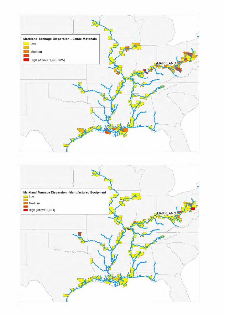


Calcasieu LockLPMS
Group
Total 2014
Tons
Tons per
Barge
Average
Distance
Cost per
Ton
Total Averted
Costs
Coal 10 245,836 1,617 1,268 $26.97 $6,629,552
Petroleum Products 20 24,988,887 2,859 542 $21.70 $542,287,348
Chemicals 30 9,078,337 2,022 846 $25.44 $230,953,087
Crude Materials 40 3,937,379 1,578 1,230 $45.66 $179,789,257
Primary Manufactured Goods 50 2,744,157 1,568 1,114 $43.73 $120,009,771
Farm Products and Food 60 843,753 1,769 1,021 $26.97 $22,753,806
Equipment 70 9,222 307 524 $26.97 $248,693
Scrap and Waste 80 626,896 1,537 259 $26.97 $16,905,741
TOTAL 42,474,467 $1,119,577,255
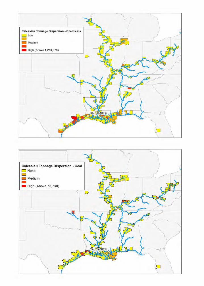
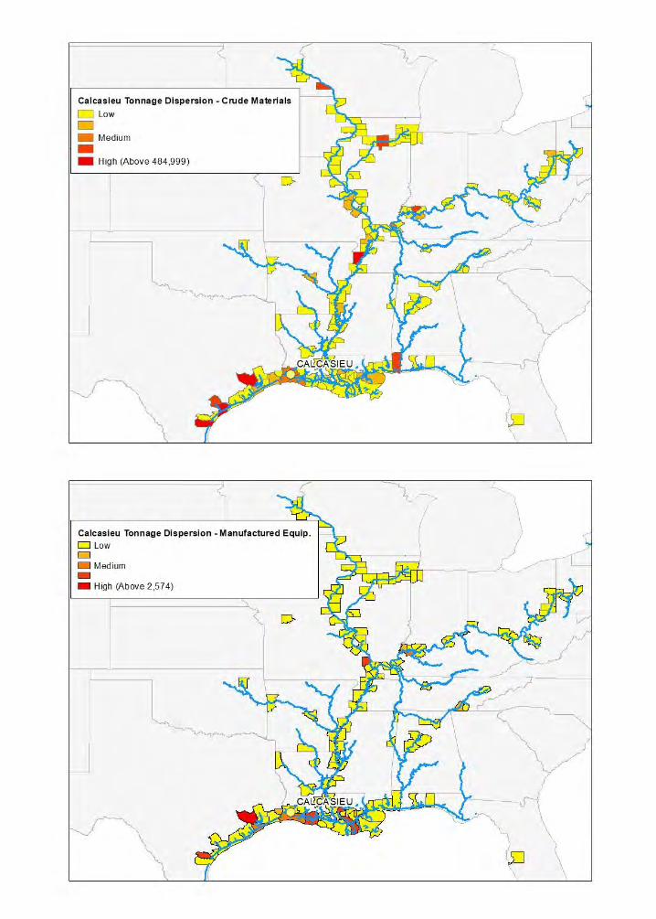
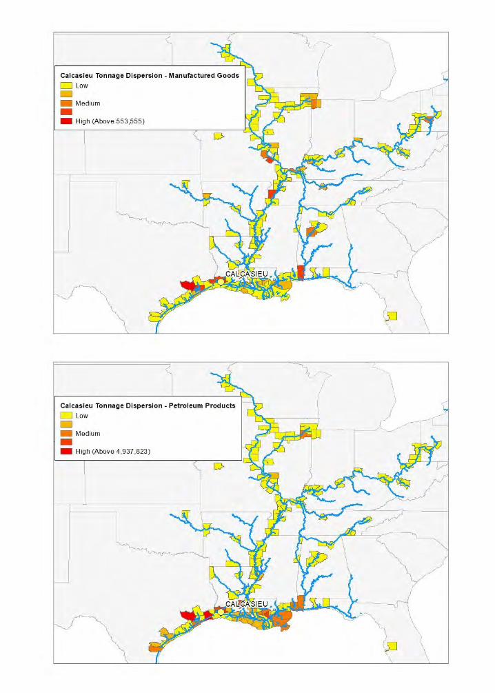

LaGrange Lock & DamLPMS
Group
Total 2014
Tons
Tons per
Barge
Average
Distance
Cost per
Ton
Total Averted
Costs
Coal 10 443,288 1,566 942 $45.77 $20,291,015
Petroleum Products 20 5,623,494 2,210 1,202 $32.53 $182,914,135
Chemicals 30 4,888,770 1,739 1,230 $51.45 $251,529,491
Crude Materials 40 3,401,419 1,552 1,270 $61.22 $208,236,345
Primary Manufactured Goods 50 3,344,289 1,513 1,056 $30.96 $103,524,351
Farm Products and Food 60 11,460,988 1,588 1,226 $81.38 $932,684,606
Equipment 70 5,632 704 1,416 $84.87 $477,986
TOTAL 29,167,880 $1,699,657,928

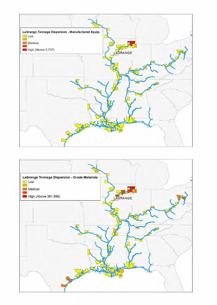

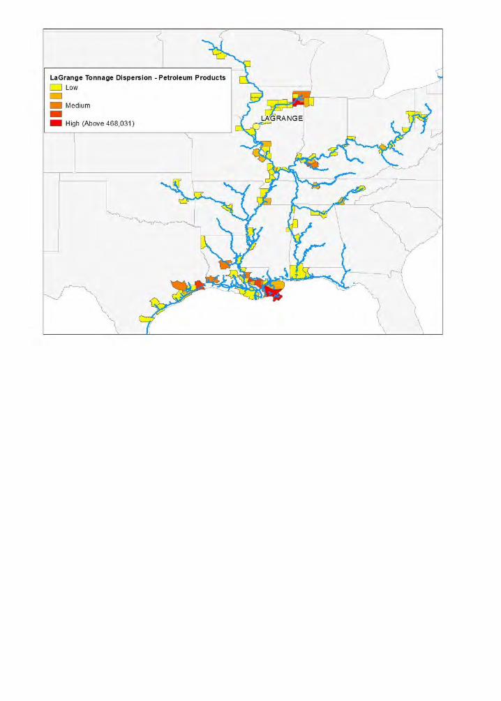

L&D 25LPMS
Group
Total 2014
Tons
Tons per
Barge
Average
Distance
Cost per
Ton
Total Averted
Costs
Coal 10 660,624 1,547 713 $38.90 $25,696,959
Petroleum Products 20 320,411 1,732 1,518 $47.14 $15,103,646
Chemicals 30 4,171,737 1,612 1,430 $59.66 $248,899,601
Crude Materials 40 3,082,613 1,568 1,488 $67.76 $208,863,996
Primary Manufactured Goods 50 1,667,149 1,677 845 $22.93 $38,225,955
Farm Products and Food 60 12,433,825 1,598 1,323 $83.16 $1,033,977,564
Equipment 70 6,602 660 1,270 $82.19 $542,606
TOTAL 22,342,961 $1,571,310,327
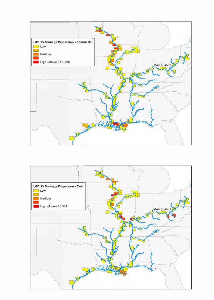
l L&D 25 Tonnage Dispersion · Chemicals
C]Low
-- Medium
-• High (Above 517,939)
_J
1 L&D 25 Tonnage Dispersion· Coal
C]Low
-• Medium
-- High (Above 60,301)

I-
