“the importance of thermodynamics on process simulation...

“The Importance of Thermodynamics on Process Simulation Modeling“

Timothy M. Zygula

Westlake Styrene Corp. 900 Hwy. 108

Sulphur, La 70664

Eric Roy

Westlake Petrochemical Corp. 900 Hwy. 108

Sulphur, La 70664

Pamela C. Dautenhahn, Ph.D., P.E.

McNeese State University College of Engineering and Technology

P.O. Box 91735 Lake Charles, La 70609-1735

"Copyright 2001 Timothy M. Zygula and Pamela C. Dautenhahn, Ph.D., P.E."

All rights reserved

Not to be uploaded to any other web site without written permission from the

copyright holder.

Distributed by

Timothy M. Zygula

NOVA Chemicals Inc. 12222 Port Road

Pasadena, TX 77507

1-281-291-1929 1-281-474-1024(Fax)

[email protected]

3e

1

“The Importance of Thermodynamics on Process Simulation Modeling”

Timothy M. Zygula


Sulphur, La 70664

Eric Roy


Sulphur, La 70664

Pamela C. Dautenhahn, Ph.D., P.E.

McNeese State University College of Engineering and Technology

P.O. Box 91735 Lake Charles, La 70609-1735

Prepared for Presentation at the The AIChE 2001 Spring National Meeting

"Copyright 2001 Timothy M. Zygula and Pamela C. Dautenhahn, Ph.D., P.E."

All rights reserved

AIChE shall not be responsible for statements or opinions contained in papers or printed in its publications.

2

ABSTRACT This paper will demonstrate the importance of choosing the correct thermodynamic package when using a process simulator to model a distillation column. The authors will present a brief background of how thermodynamics are used in distillation design. The authors will then present a test case comparing operating data and design details of a commercial hydrocarbon column with results from three different process simulation packages. The test case will be used to demonstrate the steps to obtain a good model using a process simulator. Finally, the authors will provide guidelines to select the correct thermodynamic method when using a process simulation package to model a distillation column.

3

Introduction There are many factors to consider when modeling or designing a distillation column using a commercial process simulation package. One of the biggest concerns is correctly choosing the thermodynamic package to use in simulation design work. This paper will present some guidelines for selecting the correct thermodynamic method when using a commercial process simulation package to model distillation equipment. The authors will present a test case comparing operating data from a commercial hydrocarbon column with results from three different process simulation packages. These cases will be used to demonstrate the steps to obtain a good model using a process simulator. SIMULATION MODELING Thermodynamic Properties Thermodynamic properties are critical to the success of a simulation model. The accuracy of a model depends on the ability of the thermodynamic package used to estimate the physical properties of the components in the system. Sometimes poor physical property data may prevent your simulation model from converging. (1) Although many typical problems in the thermodynamics may arise from having missing physical property parameters for the compounds in the system, this paper is going to concentrate on using the simulation packages without any adjustments for these missing parameters. The purpose of this paper is to compare results of various thermodynamic packages for a specific system. The thermodynamic packages were chosen on the expectation that they would be either good or not so good methods for the compounds being used in the commercial column. Vapor-Liquid Equilibrium In the analysis of distillation columns and other vapor-liquid separation processes the compositions of multicomponent vapor and liquid mixtures in equilibrium must be estimated. The basis for vapor-liquid equilibrium calculations is the following relationship.

),,(),,( iV

iiL

i yPTfxPTf = where: T- temperature, °F

P- pressure, psia xi- liquid phase mole fraction yi- vapor phase mole fraction fi- fugacity of a species in a mixture

4

In order to calculate the fugacity of a species in the vapor phase an equation of state must be used. However, there are two distinct methods for calculating the fugacity of a species in the liquid phase. An activity coefficient model or an equation of state can be applied. (2) The activity coefficient model can be used for liquid mixtures of all species. The activity coefficient model does not incorporate the density of the liquid and does not do a good job of describing an expanded liquid that occurs near the vapor liquid critical point of the mixture. Problems can also occur when using two different models for the liquid phase and the vapor phase. For example, when using an activity coefficient model for the liquid phase and an equation of state for the vapor phase the properties of the two phases may not become identical. When this occurs the vapor liquid critical region behavior is predicted incorrectly. (2) When using an identical equation of state to calculate vapor and liquid phase properties good phase equilibrium predictions can be made over a wide range of temperatures and pressures. These equations also do very well predicting conditions at the critical region. Not only can the phase compositions be predicted from an equation of state but other physical properties can be predicted as well. Some of the properties that can be predicted using an equation of state are densities and enthalpies. However, this is only possible for hydrocarbon mixtures, inorganic gases, and a few other materials. (2) The most common method is to use an equation of state to predict vapor phase compositions and properties and using an activity coefficient model to predict liquid phase compositions and properties. This way insures that the physical properties for both the liquid phase and the vapor phase can be calculated with reasonable accuracy. Equations of State The mathematical relationship between pressure, temperature, volume and composition is called the equation of state. Most equations of state are pressure explicit. (3) Thermodynamic properties can be predicted over a wide temperature and pressure range, including the critical region, by equations of state. When molecules are relatively small and nonpolar, they have been proven to be effective for vapor-liquid equilibrium calculations. However, the equations of state tend to be inaccurate for strongly hydrogen-bonding mixtures or substances with more complex molecular structure. (4,5) Many of the equations of state give similar results in estimating the vapor-liquid equilibrium. Bubble point pressure estimations of hydrocarbons and gases have been found to be within five percent and estimations based on binary interaction parameters have been within about 15 % accuracy. (4) In general, the variations in accuracy between the equations of state are subtle. One equation might be best for a narrow range of applications, while another equation might be more appropriate for another range of applications. (4)

5

Activity Coefficient Method An ideal mixture can either be liquid or gaseous which is defined by the following relationships:

( , , ) ( ,( , , ) ( , )

IMi i i

IMi i i

)H T P x H T PV T P x V T P

=

=

where: T- temperature, °F

P- pressure, psia xi- liquid phase mole fraction

iV - Partial Molar Volume, ith Component

iH - Enthalpy Per Mole, ith Component IMiH - Enthalpy Per Mole, Ideal Mixture IM

iV - Partial Molar Volume, ideal Mixture In an ideal liquid solution, the liquid fugacity of each component in the mixture is directly proportional to the mole fraction of the component. The ideal solution assumes that all molecules in the liquid solution are identical in size and are randomly distributed. This assumption is valid for mixtures containing molecules of similar size and character. (3) In general, you can expect non-ideality in mixtures of unlike molecules. Either the size or shape or the intermolecular interactions between components may be dissimilar. These differences are called size and energy asymmetry. Energy asymmetry occurs between polar and non-polar molecules and also between different polar molecules. An example is a mixture of alcohol and water. (3) The activity coefficient represents the deviation of the mixture from ideality. The activity of a component at some temperature, pressure and composition is defined as the ratio of the fugacity of the component at actual conditions over the fugacity of the component at standard conditions. (3)

),,(/),,(),,( ooiii xPTfxPTfxPTa =

where ai – component activity

T – temperature at actual conditions P – pressure at actual conditions x – liquid mole fraction at actual conditions.

Note: The superscript “o” indicates at standard state.

6

The liquid activity models are designed to have more flexibility by having more adjustable parameters and allow the free energy curve to be accurately tuned for magnitude and skewness. One of the key features of these models is treating liquids differently than vapors. The liquids are evaluated as deviations from ideal-solution behavior, where as the vapors are evaluated as deviations from ideal-gas behavior. (4) Peng Robinson Equation The Peng Robinson equation is an equation of state that is generally good for ideal hydrocarbon systems not operating near the critical region. The Peng Robinson equation does not do a good job of matching the experimental data in the critical region. The equation calculates a larger two-phase region than what was generated through experimental data. One reason that might explain this deviation is in the critical region density fluctuations contributes strongly to thermodynamic properties. These fluctuations are ignored in the Peng Robinson equation. To incorporate this into this equation would be extremely difficult. (3) NRTL & Van Laar Equations The NRTL (Non-Random Two Liquid) equation is a three-parameter equation that can be used for both liquid-liquid and vapor-liquid equilibria correlations. The strength of the NRTL equation is for highly non-ideal systems. The NRTL equation often provides a good representation of highly non-ideal mixtures, polar compounds and partially immiscable systems. The NRTL equation provides good representation of experimental data if care is exercised in data reduction to obtain the adjustable parameters in the equation. (3) The Van Laar is a two-parameter equation that is good for moderately non-ideal systems. The Van Laar equation should be used for relatively simple non-polar liquids. However, this equation has been empirically fit to represent the activity coefficients of complex liquids. The Van Laar equation is a popular equation to use because it is easy to mathematically manipulate. (3) For moderately non-ideal systems, the NRTL equation does not offer a significant advantage over the Van Laar and the three-suffix Margules equation. SIMULATION MODEL Many times when simulating a distillation column the simulation model may not converge or, if it does converge, the model does not match plant data. After confirming that the input data are correct one may determine that the immediate answer to the problem is that “I have chosen the wrong thermodynamic package for my system”. Then you begin switching between thermodynamic packages to try to get your simulation model to work. However, once the simulation has converged or you have matched your plant data does not mean that your model is correct. Thermodynamic packages are constructed for

7

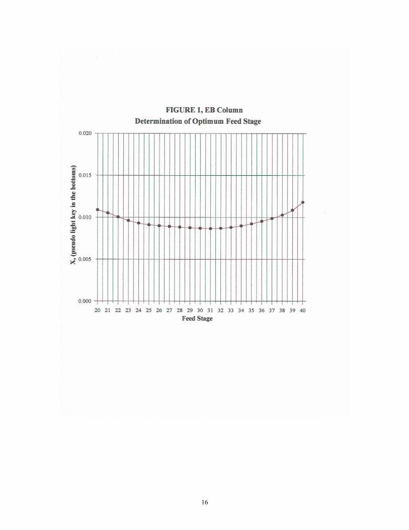
specific applications. Some thermodynamic packages are good for highly non-ideal systems while others are not. The thermodynamic model used might be outside its recommended range. For example, the temperature or pressure range or both ranges are exceeded. In many cases thermodynamic models are extrapolated to ranges beyond the data they have for that model. However, any time a model is extrapolated outside its range the results are questionable until evaluated for validity. Physical properties are critical to the success and accuracy of a simulation model. Poor physical property data may prevent your simulation model from converging or matching operating data. In this paper, three different thermodynamic packages are used for estimating the physical property data to match the data for a commercial hydrocarbon tower. In addition, three simulation packages are used to demonstrate how the results from the same thermodynamic packages may vary from simulator to simulator. The variations from simulator to simulator represent slightly different property estimations or values for the components in the system. The purpose of using different simulators is to demonstrate that there are variations and one should always analyze the results from a simulator for accuracy and reasonableness. (7) TEST CASE The results from a test case, which is a commercial ethylbenzene recovery tower, will be examined. Plant data from this tower were compared with results from three process simulation packages using three thermodynamic packages. For each of the thermodynamic packages, it was desired to match the external material and composition data reasonably well. Then the rest of the data, including the internal vapor and liquid flow rates, equilibrium data, and column diameter estimations were compared for similarities and differences. The ethylbenzene recovery tower separates ethylbenzene from heavier materials. The feed was a 45% vapor mixture at 38.6 psia pressure. Since operational data were available the simulations were run to match the operational data. The desired products contained 99.4 percent ethylbenzene in the distillate and 85 percent heavy materials in the bottoms. Several thermodynamic models were chosen for use in the simulation runs on this tower. These models included Peng Robinson, Non-Random –Two-Liquid (NTRL) and Van Laar. Feed Stage Optimization and McCabe-Thiele Diagram Development To determine the optimum feed stage, simulation runs were performed at several different feed positions. In the simulation runs, the material balance, reflux ratio, and total number of stages were kept constant. The feed tray was varied and the light key component composition in the bottoms was determined. Then a concentration versus feed stage plot was created and is given in Figure 1. The optimum feed stage is where the minimum of the curve occurs. From Figure 1 it can be seen that there are several stages in which the minimum value of the light key is approximately the same. Based on these data, the

8

optimum feed stage was chosen as stage 30, which also corresponded to the expected efficiency for the column. All of the simulation results presented with the pseudo McCabe-Thiele diagram used stage 30 as the feed stage. For each of the simulation runs a pseudo McCabe-Thiele diagram was developed. The pseudo McCabe-Thiele diagram was developed by using the mole fraction data for the light key and all lighter components calculated for each stage by the simulations. The equilibrium data and the operating lines were determined from these data. The pseudo McCabe-Thiele diagram helps one identify pinched regions, mislocated feed points, over refluxing or reboiling, or where feed or intermediate heat exchangers are needed. (6) Test Case Results The results from the simulation runs were compared to the plant operational data. The feed pressure was specified as 38.6 psia and the feed vapor fraction was specified as 0.4544. The pressure profile was held constant in all simulation runs. In addition, the simulation runs held constant the feed rate at 67,995 lbs/hr, the reflux rate at 174736 lbs/hr, and the ethylbenzene (EB) composition in the bottoms at 0.671 weight percent. Theoretical stages were used and the number was based on what is believed to be the overall efficiency of the tower. Figures 2, 3, and 4 show the comparison of the simulation results of the commercial ethylbenzene recovery column. Peng Robinson Simulation Runs Figure 2 shows a comparison of equilibrium data from simulator A, B and C using the Peng Robinson model. The equilibrium data for simulators A and C are almost identical. The equilibrium curves as well as the operating lines lie on top of each other. This indicates that the results from the two simulation packages will be very close. The equilibrium curve for simulator B is consistently higher than simulators A and B. This shift in the equilibrium curve indicates that separation is easier and that the internal traffic in the column is lower. The operating line from simulator B is identical to the operating lines from simulators A and C. A comparison of the simulated results using the Peng Robinson model is given in Table 1. The data in Table 1 show good agreement between the plant data and the simulated results. There is only a one-degree difference between the overhead temperature measured in the plant and the temperature calculated in the simulation runs. The feed temperature calculated for simulator A and B is between one and two degrees less than plant data. The feed temperature calculated by simulator C is slightly more than two degrees cooler than plant data. There is some slight variation in the calculated results for the EB distillate composition and heavies’ composition in the bottom. However, all of the results are considered to reasonably match plant data.

9

Table 1. Comparison of Key Data using Peng Robinson

Ovhd

Temp °F

Btm Temp, °F

Reboiler Duty, mmBtu/Hr

EB Comp. Distillate Wt%

Feed Temp, °F

Heavies in the Bottom Wt%

Plant Data 334 426 99.46 364 85.69 Simulator A

333 427 2.76 99.40 362.1 86.26

Simulator B 333 430 2.77 99.46 362.6 86.29 Simulator C

332 427 2.77 99.43 361.8 86.29

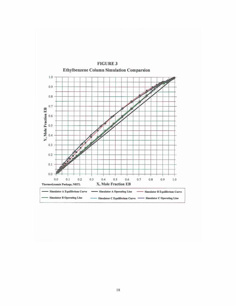
NRTL Simulation Runs Figure 3 shows a comparison of equilibrium data from simulator A, B and C using the NRTL model. The equilibrium data for simulators A and C are almost identical. The equilibrium curves as well as the operating lines lie on top of each other. This indicates that the results from the two simulation packages will be very close. The equilibrium curve for simulator B at the bottom of the column is below the equilibrium line for simulators A and C. Then as you go up the column it cross the equilibrium line of simulators A and C. This shift in the equilibrium curve indicates that there is going to be big differences in the internal traffic above and below the feed in the results from simulator B. The operating line from simulator B is identical to the operating lines from simulators A and C. A comparison of the simulated results using the NRTL model is given in Table 2. There is good agreement in the simulated results presented in Table 2. The overhead temperature, feed temperature, EB distillate composition and heavies’ composition in the bottoms simulated results match plant data very well. The bottom temperature has the most variation with the temperatures ranging from –15 degrees to +15 degrees with respect to the plant measurement.

Table 2. Comparison of Key Data using NRTL

10

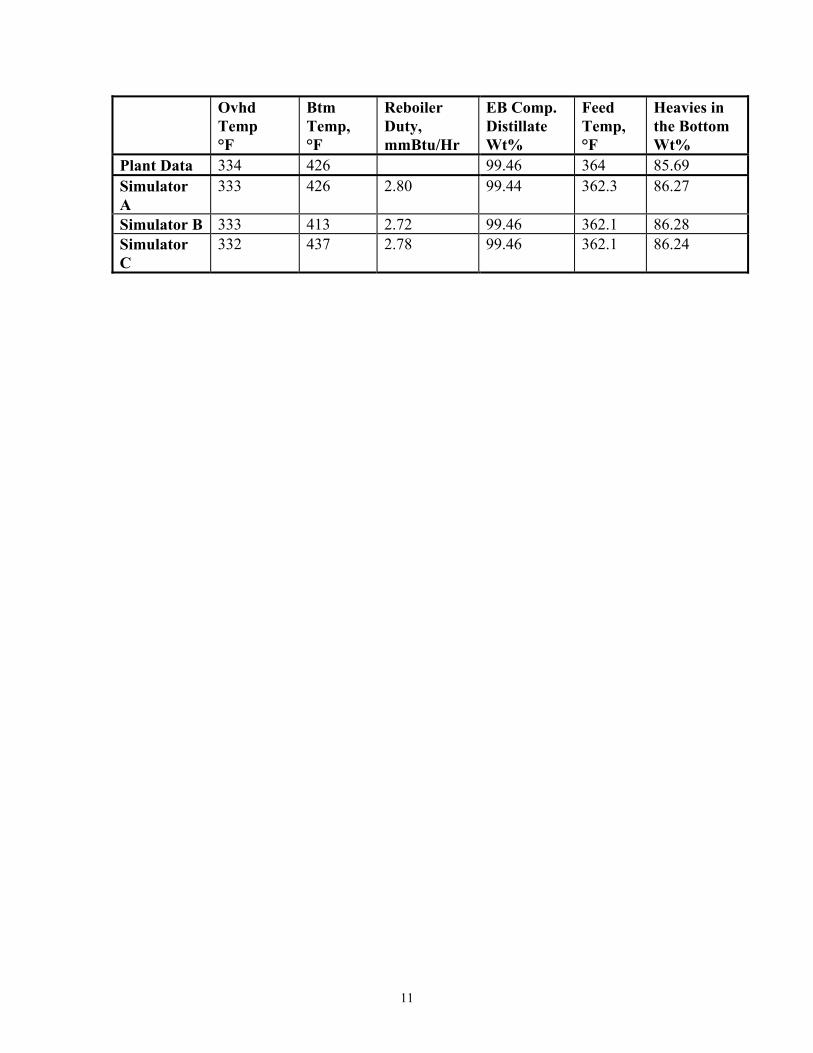
Ovhd Temp °F

Btm Temp, °F



Feed Temp, °F



333 426 2.80 99.44 362.3 86.27


332 437 2.78 99.46 362.1 86.24

11

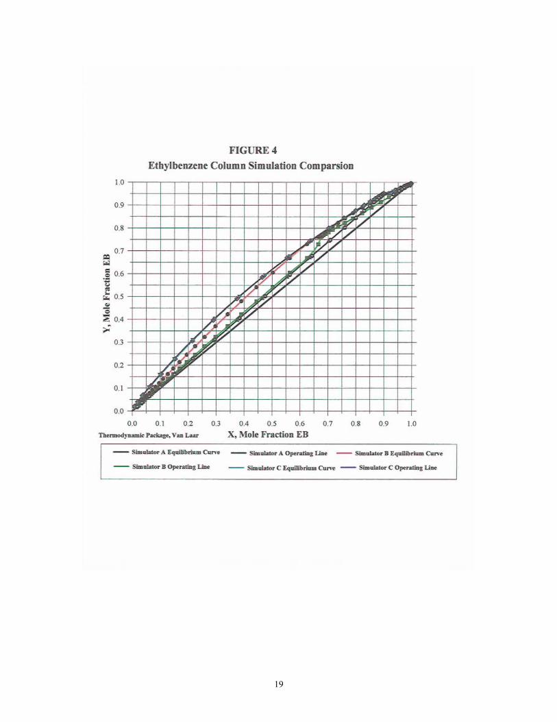
Van Laar Simulation Runs Figure 4 shows a comparison of equilibrium data from simulator A, B and C using the Van Laar model. The trends in this diagram are the same as seen in the NTRL diagram. Simulators A and C give similar results while Simulator B varies like it did with the NRTL method. A comparison of the simulated results using the Van Laar model is given in Table 3. The data in Table 3 shows good agreement between the plant data and the simulated results. There is only a one-degree difference between the overhead temperature measured in the plant and the temperature calculated in the simulation runs for simulator A and B. Simulator C shows a two-degree difference in overhead temperature. There is an approximate ± 3-degree difference in feed temperatures calculated for simulators A and B with respect to the plant data. However, simulator C matched the feed temperature data almost exactly. There is some slight variation in the calculated results for the EB distillate composition and heavies’ composition in the bottom. The results given by simulator B did not match the EB composition in the distillate as well as the others.

Table 3. Comparison of Key Data using Van Laar Ovhd

Temp °F

Btm Temp, °F



Feed Temp, °F



333 425 2.80 99.46 362.1 86.27


332 438 2.78 99.47 364.6 86.24

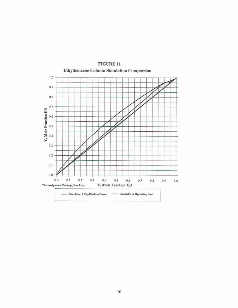
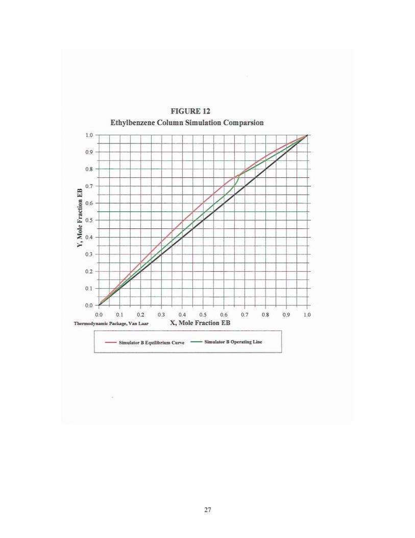
Equilibrium Curve Discussion Figures 5 –13 provide the equilibrium and operating curves for each of the individual runs. There appears to be a pinch point at the top of the equilibrium profile in all of the simulations. This pinch point is near the feed stage. The column does most of its separation below the feed. Typically this type of pinch indicates that there is a mislocated feed point. The feed point should be where the q-line intersects the equilibrium curve. This is generally the rule in binary distillation. However, it is not always true in multicomponent distillation. The optimum feed stage plot, Figure 1, suggested the optimum feed stage is used in the simulation runs. (6) Therefore, a pinch point appears in the equilibrium diagrams that can’t be explained by bad feed point location or system limitation. The pinch point tends to shift in simulator B when the Van Laar model is used. In ternary and higher component systems, the curvature in the operating lines will also sometimes cause curvature in the equilibrium

12

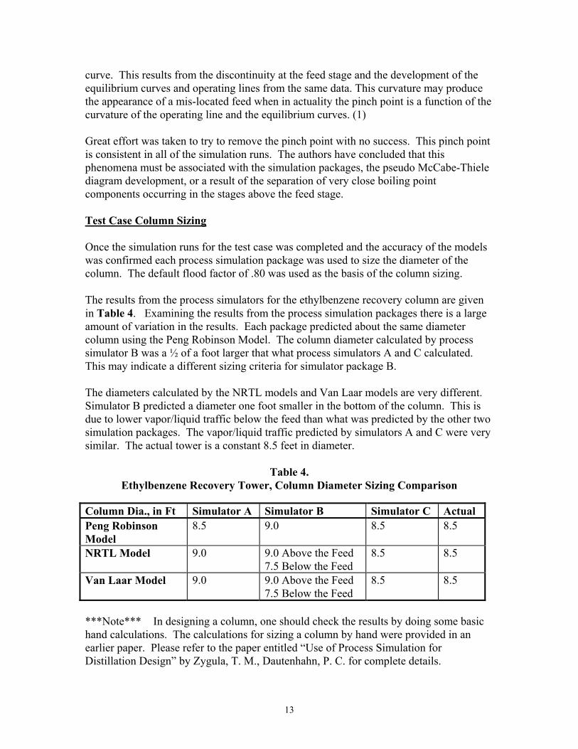
curve. This results from the discontinuity at the feed stage and the development of the equilibrium curves and operating lines from the same data. This curvature may produce the appearance of a mis-located feed when in actuality the pinch point is a function of the curvature of the operating line and the equilibrium curves. (1) Great effort was taken to try to remove the pinch point with no success. This pinch point is consistent in all of the simulation runs. The authors have concluded that this phenomena must be associated with the simulation packages, the pseudo McCabe-Thiele diagram development, or a result of the separation of very close boiling point components occurring in the stages above the feed stage. Test Case Column Sizing Once the simulation runs for the test case was completed and the accuracy of the models was confirmed each process simulation package was used to size the diameter of the column. The default flood factor of .80 was used as the basis of the column sizing. The results from the process simulators for the ethylbenzene recovery column are given in Table 4. Examining the results from the process simulation packages there is a large amount of variation in the results. Each package predicted about the same diameter column using the Peng Robinson Model. The column diameter calculated by process simulator B was a ½ of a foot larger that what process simulators A and C calculated. This may indicate a different sizing criteria for simulator package B. The diameters calculated by the NRTL models and Van Laar models are very different. Simulator B predicted a diameter one foot smaller in the bottom of the column. This is due to lower vapor/liquid traffic below the feed than what was predicted by the other two simulation packages. The vapor/liquid traffic predicted by simulators A and C were very similar. The actual tower is a constant 8.5 feet in diameter.

Table 4. Ethylbenzene Recovery Tower, Column Diameter Sizing Comparison

Column Dia., in Ft Simulator A Simulator B Simulator C Actual Peng Robinson Model

8.5 9.0 8.5 8.5

NRTL Model 9.0 9.0 Above the Feed 7.5 Below the Feed

8.5 8.5

Van Laar Model 9.0 9.0 Above the Feed 7.5 Below the Feed

8.5 8.5

***Note*** In designing a column, one should check the results by doing some basic hand calculations. The calculations for sizing a column by hand were provided in an earlier paper. Please refer to the paper entitled “Use of Process Simulation for Distillation Design” by Zygula, T. M., Dautenhahn, P. C. for complete details.

13

Conclusions The results from these runs have shown that there will be variations between thermodynamic packages within a simulator and the same thermodynamic package between simulators. It is important to analyze the results for each system based on an appropriate thermodynamic method associated with the simulation package. Recommendations An equation of state can be used over a wide range of temperatures and pressures, including the subcritical and supercritical regions. Equations of state are typically used for ideal or slightly non-ideal systems, thermodynamic properties for both the vapor and liquid phases can be computed with a minimum amount of component data. Equations of state are suitable for modeling hydrocarbon systems with light gases. Equations of state are not capable of properly representing highly non-ideal systems, such as alcohol and water systems For the best representation of non-ideal systems an activity coefficient model may be the best. One draw back of an activity coefficient model is that you may need to obtain binary interaction parameters from regression of experimental vapor-liquid equilibrium (VLE) data. Table 5 provides some choices for deciding which thermodynamic model to try when modeling distillation columns. There are a few things to keep in mind when looking at this chart. Non-polar fluids may be modeled with an equation of state. Polar fluids are best modeled with a fitted activity coefficient model. Some systems have specific thermodynamic models designed especially for that kind of system. For example, there are some thermodynamic packages that specifically model electrolytic solutions. There are other thermodynamic packages that model alcohol systems and amine systems. These facts should be taken into account when trying to choose a thermodynamic model. (3)

Table 5 Thermodynamic Model Selection Table (5)

System Thermodynamic Model All Gases, Non-Polar Solutions Peng Robinson, SRK Moderately Non-Ideal, Polar Solutions NRTL, Wilson, Van Laar Highly Non-Ideal, Polar Systems NRTL, UNIQUAC ***Note*** When using the following equations, NRTL, Wilson, and Van Laar, you should make sure that all of the Binary Interaction Parameters are present before using the equation to obtain the best results. (5)

14

REFERENCES 1. Zygula, T. M., Dautenhahn, P. C. Ph.D., P.E. “Use of Process Simulation for Distillation Design” AIChE Spring

National Conference, March 2000, Atlanta, Georgia. 2. Sandler, Stanley. I. Chemical And Engineering Thermodynamics, John Wiley & Sons, Inc., New York, 1989. 3. Prausnitz, J. M., Lichtenthaler, R. N., Azevedo, E. G. Molecular Thermodynamics of Fluid-Phase Equilibria,

Third Edition, Prentice Hall Inc., New Jersey, 1999. 4. Elliot, T. Richard, Lira, Carl T. Introductory Chemical Engineering Thermodynamics, Prentice Hall Inc., New

Jersey, 1999. 5. Kyle, B. G. Chemical and Process Thermodynamics, Third Edition, Prentice Hall Inc., New Jersey, 1999. 6. Kister, H. Z. Distillation Design, McGraw-Hill Book Company Inc., New York, 1992. 7. Mathias, P. M., Klotz, H. C. “Take a Closer Look at Thermodynamic Property Models” Chemical Engineering

Progress, June 1994, Pg. 67-75

15

“the importance of thermodynamics on process simulation...

Documents