the independent components of natural scenes are …the "independent components" of...

Pergamon PII: S0042-6989(97)00121-1

Vision Res., Vol. 37, No. 23, pp. 3327-3338, 1997 © 1997 Elsevier Science Ltd. All rights reserved

Printed in Great Britain 0042-6989/97 $17.00 + 0.00

The "Independent Components" of Scenes are Edge Filters ANTHONY J. BELL,* t TERRENCE J. SEJNOWSKI*

Received 16 July 1996; in revised form 9 April 1997

Natural

It has previously been suggested that neurons with line and edge selectivities found in primary visual cortex of cats and monkeys form a sparse, distributed representation of natural scenes, and it has been reasoned that such responses should emerge from an unsupervised learning algorithm that attempts to find a factorial code of independent visual features. We show here that a new unsupervised learning algorithm based on information maximization, a nonlinear "infomax" network, when applied to an ensemble of natural scenes produces sets of visual filters that are localized and oriented. Some of these filters are Gabor-like and resemble those produced by the sparseness-maximization network. In addition, the outputs of these filters are as independent as possible, since this infomax network performs Independent Components Analysis or ICA, for sparse (super-gaussian) component distributions. We compare the resulting ICA filters and their associated basis functions, with other decorrelating filters produced by Principal Components Analysis (PCA) and zero-phase whitening filters (ZCA). The ICA filters have more sparsely distributed (kurtotic) outputs on natural scenes. They also resemble the receptive fields of simple cells in visual cortex, which suggests that these neurons form a natural, information-theoretic coordinate system for natural images. © 1997 Elsevier Science Ltd

Information theory Independent components Neural network learning

INTRODUCTION

Both the classic experiments of Hubel & Wiesel (1968) on neurons in visual cortex, and several decades of theorizing about feature detection in vision (Marr & Hildreth, 1980), have left open the question most succinctly phrased by Barlow & Tolhurst (1992) "Why do we have edge detectors?"

That is: are there any coding principles which would predict the formation of localized, oriented receptive fields? Barlow's answer was that edges are suspicious coincidences in an image. Since the mathematical framework for analysing such "coincidences" is Informa- tion Theory (Cover & Thomas, 1991), Barlow was thus led to propose that our visual cortical feature detectors might be the end result of a "redundancy reduction" process (Barlow, 1989; Atick, 1992), in which the activation of each feature detector is supposed to be as "statistically independent" from the others as possible. Such a "factorial code" potentially involves dependen- cies of all orders, but most studies have used only the

*Howard Hughes Medical Institute, Computational Neurobiology Laboratory, The Salk Institute, 10010 N. Torrey Pines Road, La Jolla, CA 92037, U.S.A.

tTo whom all correspondence should be addressed [E-mail tony@- salk.edu].

second-order statistics required for "decorrelating" the outputs of a set of feature detectors.

A variety of Hebbian feature-learning algorithms for decorrelation have been proposed (Linsker, 1992; Miller, 1988; Oja, 1989; Sanger, 1989; Frldi~ik, 1990; Atick & Redlich, 1993), but in the absence of particular external constraints the solutions to the decorrelation problem are non-unique (see: Decorrelation and Independence). One popular decorrelating solution is Principal Components Analysis (PCA) but the principal components of natural scenes amount to a global spatial frequency analysis (Hancock et al., 1992). Therefore, second-order statistics alone do not suffice to predict the formation of localized edge detectors.

Additional constraints are required. Field (1987, 1994) has argued for the importance of sparse, or "minimum entropy", coding (Barlow, 1994), in which each feature detector is activated as rarely as possible. This has led to feature-learning algorithms (Intrator, 1992) with a "projection pursuit" (Huber, 1985) flavour, the most successful of which has been the Olshausen & Field (1996) demonstration of the self-organization of local, oriented receptive fields using a sparseness criterion.

Here we present results similar to those of Olshausen and Field, using a direct information-theoretic criterion which maximizes the joint entropy of a nonlinearly transformed output feature vector. We have previously

3327

3328 A.J. BELL and T. J. SEJNOWSKI

U

filters

W image patch, X

image J ensemble

basis functions

s ) ( ) O , . ~ - - - - _ c a u s e s

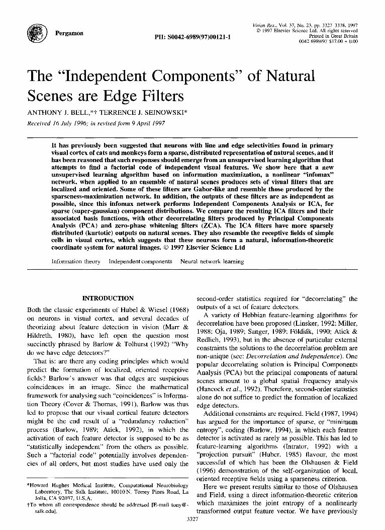
FIGURE 1. The Blind Linear hnage Synthesis model (Olshausen & Field, 1996). Each patch, x, of an image is viewed as a linear combination of several (here three) underlying basis functions, given by the matrix A, each associated with an element of an underlying vector of "causes", s. In this paper, causes are viewed as statistically independent " image sources". The causes are recovered (in a vector u) by a matrix of filters, W, more loosely "receptive fields", which attempt to invert the unknown mixing

of unknown basis functions constituting image formation.

demonstrated the ability of this nonlinear information maximization process (Bell & Sejnowski, 1995a) to find statistically independent components to solve the problem of separating mixed audio sources (Jutten & Hrrault, 1991). This "Independent Components Analy- sis" (ICA) problem (Comon, 1994) is equivalent to Barlow's redundancy reduction problem, therefore, if Barlow's reasoning is correct, we would expect the ICA solution to yield localized edge detectors.

That it does so is the primary result of this paper. The secondary result is that the outputs of the resulting filters are indeed, more sparsely distributed than those of other decorrelating filters, thus supporting some of the arguments of Field (1994), and helping to explain the results of Olshausen's network from an information-theoretic point of view.

We will return to the issues of sparseness, noise and higher-order statistics in the Discussion. First, we describe more concretely the filter-learning problem. An earlier account of the application of these techniques to natural sounds appears in Bell & Sejnowski (1996).

B L I N D S E P A R A T I O N O F N A T U R A L I M A G E S

The starting point is that of Olshausen & Field (1996), depicted in Fig. 1. A perceptual system is exposed to a series of small image patches, drawn from one or more larger images. Imagine that each image patch, represented by the vector x, has been formed by the linear combination of N basis functions. The basis functions

form the columns of a fixed matrix, A. The weighting of this linear combination (which varies with each image) is given by a vector, s. Each component of this vector has its own associated basis function, and represents an underlying "cause" of the image. The "linear image synthesis" model is therefore given by:

x = As. ( l)

which is the matrix version of the set of equations xi = ~N_ 1 aijsj, where each xi represents a pixel in an image, and contains contributions from each one of a set of N image "sources", s/, linearly weighted by a coefficient, aij.

The goal of a perceptual system, in this simplified framework, is to linearly transform the images, x, with a matrix of filters, W, so that the resulting vector:

u = W x (2)

recovers the underlying causes, s, possibly in a different order, and rescaled. Representing an arbitrary permuta- tion matrix (all zero except for a single "one" in each row and each column) by P, and an arbitrary scaling matrix (non-zero entries only on the diagonal) by S, such a system has converged when:

u = WAs = PSs. (3)

The scaling and permuting of the causes are arbitrary, unknowable factors, so we will consider the causes to be defined such that PS = I (the identity matrix). Then the basis functions (columns of A) and the filters which

THE "INDEPENDENT COMPONENTS" OF NATURAL SCENES ARE EDGE FILTERS 3329

recover the causes (rows of W) have the simple relation: W = A 1.

All that remains in defining an algorithm to learn W (and thus also A) is to decide what constitutes a "cause". A number of proposals are considered in the Discussion, however, in the next two sections, we concentrate on algorithms producing causes which are decorrelated, and those attempting to produce causes that are statistically independent.

DECORRELATION AND INDEPENDENCE

The matrix, W, is a decorrelating matrix when the covariance matrix of the output vector, u, satisfies:

(uuTI = diagonal matrix. (4)

In general, there will be many W matrices which decorrelate. For example, in the case of equation (2), when (uu T) = I, then:

w T w : (xxT) 1 (5)

which clearly leaves freedom in the choice of W. There are, however, several special solutions to equation (5).

The orthogonal (global) solution [ W W y = S]

Principal Components Analysis (PCA) is the orthogonal solution to equation (4). The principal components come from the eigenvectors of the covariance matrix, which are the columns of a matrix, E, satisfying:

EDE "1 : <xxT) (6)

where D is the diagonal matrix of eigenvalues. Substitut- ing equation (6) into equation (5) and solving for W gives the PCA solution, Wp:

Wp = D-~E T. (7)

This solution is unusual in that the filters (rows of We) are orthogonal, so that w W T = D -1, a scaling matrix. These filters thus have several special properties:

1. The PCA filters define orthogonal directions in the vector space of the image.

2. The PCA basis functions (columns of Ap, or rows of w p T - - s e e Fig. 1) are just scaled versions of the PCA filters (rows of We). This latter property is true because W W T = D-1 means that W -T = DW.

3. When the image statistics are stationary (Field, 1994), the PCA filters are global Fourier filters, ordered according to the amplitude spectrum of the image.

Example PCA filters are shown in Fig. 3(a).

The symmetrical (local) solution I W W T = W 2]

If we force W to be symmetrical, so that W T = W, then the solution, Wz to equation (5) is:

Wz = (xxT) -1/2. (8)

Like most other decorrelating filters, but unlike PCA, the basis functions and the filters coming from Wz will be

W - s p a c e

~ U E N C Y

~ / ~ ZCA

/ ~ J SEMI-LOCAL

O e c o r r e l a t i n g W ' s : WTW = <x xT71

FIGURE 2. A schematic depiction of weight-space. A subspace of all matrices W, here represented by the loop (of course it is a much higher- dimensional closed subspace), has the property of decorrelating the input vectors, x. On this manifold, several special linear transforma- tions can be distinguished: PCA (global in space and local in frequency), ZCA (local in space and global in frequency), and ICA. a privileged decorrelating matrix which, if it exists, decorrelates higher- as well as second-order moments. ICA filters are localized, but

not down to the single pixel level, as ZCA filters are (see Fig. 3.)

different from each other, and neither will be orthogonal. We might call this solution ZCA, since the filters it produces are zero-phase (symmetrical). ZCA is in several ways the polar opposite of PCA. It produces local (centre-surround type) whitening filters, which are ordered according to the phase spectrum of the image. That is, each filter whitens a given pixel in the image, preserving the spatial arrangement of the image and flattening its frequency (amplitude) spectrum. Wz is related to the transforms described by Goodall (1960) and Atick & Redlich (1993).

Example ZCA filters and basis functions are shown in Fig. 3(b).

The independent (semi-local) solution [fu(u) =

Another way to constrain the solution is to attempt to produce outputs which are not just decorrelated, but statistically independent, the much stronger requirement of Independent Components Analysis, or ICA (Jutten & Hrrault, 1991; Comon, 1994). The ui are independent when their probability distribution, fu, factorizes as follows: f u (u) = Hi fuiui, equivalently, when there is zero mutual information between them: I(ui,uj) = O, V i # j. A number of approaches to ICA have some relations with the one we describe below, notably Cardoso & Laheld (1996), Karhunen et al. (1996), Amari et al. (1996), Cichocki et al. (1994) and Pham et al. (1992). We refer the reader to these papers, to the two above, and to Bell & SejnowskJ (1995a) for further background on ICA.

As we will show, in the Results, ICA on natural images produces decorrelating filters which are sensitive to both phase (locality) and frequency information, just as in transforms involving oriented Gabor functions (Daug- man, 1985) or wavelets.* They are, thus, semi-local,

*See the Proceedings of IEEE, 84, 4, April 199~-a special issue on wavelets.


depicted in Fig. 2 as partway along the path from the local (ZCA) to the global (PCA) solutions in the space of decorrelating solutions.

Example ICA filters are shown in Fig. 3(d) and their corresponding basis functions are shown in Fig. 3(e).

AN ICA ALGORITHM

It is important to recognize two differences between finding an ICA solution, Wt, and other decorrelation methods: (i) there may be no ICA solution; and (ii) a given ICA algorithm may not find the solution even if it exists, since there are approximations involved. In these senses, ICA is different from PCA and ZCA, and cannot be calculated analytically, for example, from second- order statistics (the covariance matrix), except in the gaussian case (when second-order statistics completely characterize the signal--see section entitled: Second- and Higher-order Statistics).

The approach developed in Bell & Sejnowski (1995a) was to maximize by stochastic gradient ascent the joint entropy, H[g(u)], of the linear transform squashed by a sigmoidal function, g. When the nonlinear function is the same (up to scaling and shifting) as the cumulative density functions (c.d.f.s) of the underlying independent components, it can be shown (Nadal & Parga, 1994)* that such a nonlinear "infomax" procedure also minimizes the mutual information between the ui, exactly what is required for ICA.

However, in most cases we must pick a nonlinearity, g, without any detailed knowledge of the probability density functions (p.d.f.s) of the underlying independent components. The resulting "mismatch" between the gradient of the nonlinearity used, and the underlying p.d.f.s may cause the infomax solution to deviate from an ICA solution. In cases where the p.d.f.s are super-gaussian (meaning they are peakier and longer-tailed than a gaussian, having kurtosis greater than 0), we have repeatedly observed, using the logistic or tanh nonlinea- rities, that maximization of H[g(u)] still leads to ICA solutions, when they exist, as with our experiments on speech signal separation (Bell & Sejnowski, 1995a). Although the infomax algorithm is described here as an ICA algorithm, a fuller understanding needs to be developed of under exactly what conditions it may fail to converge to an ICA solution.

The basic infomax algorithm changes weights according to the entropy gradient. Defining Yi = g(ui) tO be the sigmoidally transformed output variables, the learning rule is then:

A W (x O H ( y ) _ E[OlnlJI] 0 w Low-J (9)

In this, E denotes expected value, y = [g(u~)...g(UN)] T,

*In a previous conference paper (Bell & Sejnowski, 1995b), we also published a proof of this result, which ought to have referenced the equivalent proof by Nadal & Parga.

and IJI is the absolute value of the determinant of the Jacobian matrix:

J = d e t [ Oyi] (10) LOxjJ

In stochastic gradient ascent we remove the expected value operator in equation (9), and then evaluate the gradient to give (Bell & Sejnowski, 1996):

m w 0<i [W T] I _~_yx T (l l )

^ ~ T where $ = [Yl-..YN] , the elements of which depend on the nonlinearity as follows:

0 0 y i 0 Oyi ?}i -- OyiOui ouilnc~ui " (12)

Amari et al. (1996) have proposed a modification of this rule, which utilizes the natural gradient rather than the absolute gradient of H(y). The natural gradient exists for objective functions which are functions of matrices, as in this case, and is the same as the relative gradient concept developed by Cardoso & Laheld (1996). It amounts to multiplying the absolute gradient by WVW, giving, in our case, the following altered version of equation (11):

0H(y) WT w = (I + :~uT)W (13)

This rule has the twin advantages over equation (11) of avoiding the matrix inverse, and of converging several orders of magnitude more quickly, for data, x, that are not prewhitened. The speed-up is explained by the fact that convergence is no longer dependent on the conditioning of the underlying basis function matrix, A, of equation (1). This is the equivariant property explained by Cardoso & Laheld (1996).

Writing equation (13) in terms of individual weights, we have:

Aw~] o( wij ~- Yi ~ Wl~]Uk. (14) k

The weighted sum non-local term in this rule can be seen as the result of a simple backwards pass through the weights from the linear output vector, u, to the inputs, x, so that each weight "knows the influence" of its input, xj.

It is also possible to write the rule in recurrent terms. As in the well known Jutten & H6rault (1991) network, or that of F61diAk (1990), we may use a feedback matrix, V, giving a network: u = x - Vu. Solving this gives u = (I + V)-~x, showing that V is just a coordinate transform of the W of equation (2). The learning rule for V is, therefore, a coordinate transform of the rule for W. This is calculated as follows. Since the relationship between W a n d V i s W = ( I + V ) - ~ , w e m a y w r i t e v = W 1 _ i . Differentiating, and using the quotient rule for matrices gives:

/xv = /x (w = -w- (Aw)w 1 (15)

Inserting equation (13) and rearranging gives the learning rule for a feedback weight matrix:


AV cx (I + V)(I + guT). (16)

In terms of an individual feedback weight, vii, this rule is:

~Vij (X ~iJ -~- Vij -{- UJ( ~i + Z Vik~k (17)

where g0 = 1 when i = j, 0 otherwise. Thus, the feedback rule is also non-local, this time involving a backwards pass through the (recurrent) weights, of quantities, yk, calculated from the nonlinear output vector, y. Such a recurrent ICA system has been further developed for recovering sources which have been linearly convolved with temporal filters by Torkkola (1996) and Lee et al. (1997).

The non-locality of the algorithm is interesting when we come to consider the biological significance of the learned filters later in this paper.

II II II II II

II

II i l !1

II i l II I!

II

II II

l i II II III II III

METHODS

We took four natural scenes involving trees, leaves and so on* and converted them to greyscale byte values between 0 and 255. A training set, {x}, was then generated of 17 595, 12 × 12 samples from the images. The training set was "sphered" by subtracting the mean and multiplying by twice the local symmetrical (zero- phase) whitening filter of equation (8):

x +--- 2Wz({X} - (x)) (18)

This removes both first- and second-order statistics from the data, and makes the covariance matrix o f x equal to 4I. This is an appropriately scaled starting point for further training since infomax [equation (13)] on raw data, with the logistic function, Yi = (1 + e x p ( - u i ) -1, produces a u-vector which approximately satisfies (uu T) = 4I. Therefore, by prewhitening x in this way, we can ensure that the subsequent transformation, u = Wx, to be learnt should approximate an orthonormal matrix (rotation without scaling), roughly satisfying the relation w T w = I (Karhunen et al. , 1996). This W moves the solution along the decorrelating manifold from ZCA to ICA (see Fig. 2).

The matrix, W, is then initialized to the identity matrix, and trained using the logistic function version of equation (13), in which equation (12) evaluates as: yi = 1 - 2yi. The training was conducted as follows: 30 sweeps through the data were performed, at the end of each of which the order of the data vectors was permuted to avoid cyclical behaviour in the learning. During each sweep, the weights were updated only after every 50 presenta- tions in order that the vectorized MATLAB code could be more efficient. The learning rate [proportionality constant in equation (13)] was set as follows: 21 sweeps at 0.001, and three sweeps at each of 0.0005, 0.0002 and 0.0001. This process took 2 hours running MATLAB on a Sparc- 20 machine, though a reasonable result for 12 × 12 filters

i t I t II i i i l I t

II l !

II III i l

II

II I t

I t

I t II II I!

l l I t II !11

II

i l Ill

*The images (gif files) used are available in the Web directory ftp:// ftp.cnl.salk.edu/pub/tony/VRimages.

5

(a) (b) (c) (d)

PCA ZCA W ICA

(e) A

7

11

15

22

37

60

63

89

109

144

II

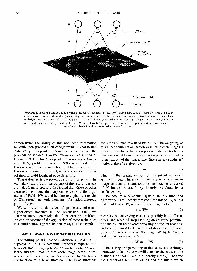
FIGURE 3. Selected decorrelating filters and their basis functions extracted from the natural scene data. Each type of decorrelating filter yielded 144 12 × 12 filters, of which we only display a subset here. Each column contains filters or basis functions of a particular type, and each of the rows has a number relating to which row of the filter or basis function matrix is displayed. (a) PCA (Wp): The first, fifth, seventh etc principal components, calculated from equation (7), showing increasing spatial frequency. There is no need to show basis functions and filters separately here since for PCA, they are the same thing. (b) ZCA (Wz): The first six entries in this column show the 1- pixel wide centre-surround filter which whitens while preserving the phase spectrum. All are identical, but shifted. The lower six entries (37, 60... 144) show the basis functions instead, which are the columns of the inverse of the Wz matrix. (c) W: the weights learnt by the ICA network trained on Wz-whitened data, showing (in descending order) the DC filter, localized oriented filters, and localized checkerboard filters. (d) W1: The corresponding ICA filters, calculated according to Wz = WWz, looking like whitened versions of the W-filters. (e) A: the corresponding basis functions, or columns of W l 1. These are the patterns which optimally stimulate their corresponding ICA filters,

while not stimulating any other ICA filter, so that WzA = I.

can be achieved in 30 min. To verify that the result was not affected by the starting condition of W = I, the training was repeated with several randomly initialized weight matrices, and also on data that were not prewhitened. The results were qualitatively similar, though convergence was much slower.

3332 A . J . BELL and T. J. SEJNOWSKI

II |

i

2

/

/

/ /

/ /

/

/ /

/ / /

/ / l /

/ l /

/

/

/ / /

/

/ /

/

/

/

/

| / /

/ /

/

/ /

/ /

/

/

/ II II / I

/ /

I / / / / /

I1 ! /

/ / /

/ / I

/ / 1

/ / /

/ /

/ / /

II /

/ /

/ /

l l l /

/ / /

/ | II | ....... i l l /

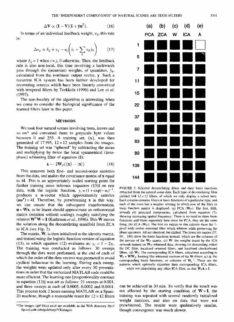
FIGURE 4. The matrix of 144 filters obtained by training on ZCA-whitened natural images. Each filter is a row of the matrix W. The ICA basis functions on ZCA-whitened data are visually the same as the ICA filters.

The full ICA transform from the raw image was calculated as the product of the sphering (ZCA) matrix and the learnt matrix: W, = WWz. The basis function matrix, A, was calculated as W~ ~. A PCA matrix, Wp, was calculated from equation (7). The original (un- sphered) data were then transformed by all three decorrelating transforms, and for each the kurtosis of each of the 144 filters was calculated, according to the formula:

K i - - { ( l ' ~ i - {bti))4) 3 ( 1 9 )

Then the mean kurtosis for each filter type (ICA, PCA, ZCA) was calculated, averaging over all filters and input data. This quantity is used to quantify the sparseness of the filters, as will be explained in the Discussion.

RESULTS

The filters and basis functions resulting from training on natural scenes are displayed in Figs 3 and 4. Figure 3

displays example filters and basis functions of each type. The PCA filters, Fig. 3(a), are spatially global and ordered in frequency. The ZCA filters and basis functions are spatially local and ordered in phase. The ICA filters, whether trained on the ZCA-whitened images, Fig. 3(c), or the original images, Fig. 3(d), are semi-local filters, most with a specific orientation preference. The basis functions, Fig. 3(e), calculated from the Fig. 3(d) ICA filters, are not local, and look like the edges that might occur in image patches of this size. Basis functions in the column Fig. 3(d) (as with PCA filters) are the same as the corresponding filters, since the matrix W (as with Wp) is orthogonal. This is the ICA-matrix for ZCA-whitened images.

In order to show the full variety of ICA filters, Fig. 4 shows, with lower resolution, all 144 filters in the matrix W. The general result is that ICA filters are localized and mostly oriented. Unlike the basis functions displayed in Olshausen & Field (1996), they do not cover a broad range of spatial frequencies. However, the appropriate comparison to make is between the ICA basis functions,


ICA, k u r t = l O . 0 4 A ~ . . . . . . . . . PCA, kur t=3 .74 / \

= .

-5

. Q ~ -10

- J

' ' ' ; 'o ' ' -1 - 3 0 - 2 0 - 1 0 1 2 0 3 0 4 0

Filter output, u i

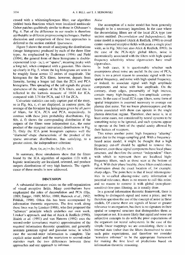
FIGURE 5. Log distributions of univariate statistics of the outputs of ICA, ZCA and PCA filters, averaged over all filters of each type. All three are approximately double-exponential distributions, but the more kurtotic ICA distribution is slightly peakier and has a longer tail, showing that it is sparser than the others. This distribution (and the 2-D ones in Fig. 6), although averaged over the outputs of all filters, are extremely similar to the distributions output by individual filters (respectively, pairs of filters)• The

only exception is the DC-filter (top left in Fig. 4) which has a more gaussian distribution.

I f u i ~ ( U i , U j ) fui(U i) L:U" I

(a) ~ (b)

• • _ o _ .

(c ) . . . . (d)

t ' , 6

(e) ( f )

FIGURE 6. Contour plots of log distributions of pairwise statistics of the outputs of ICA, ZCA and PCA filters. Left column: joint log distributions averaged over all pairs of output filters of each type, and all images• Right column: product of marginal (univariate) distributions. The ICA solution best satisfies the independence criterion that the joint distribution has the same form

as the product of the marginal distributions.

*The definition of "localized" causes some ambiguity here. While our ICA basis functions contain non-zero values all over the domain of the filter, their "contrast energy" occurs along one oriented local patch. PCA filters, on the other hand, are "more non-local" since neither of these conditions are satisfied•

a n d t he b a s i s f u n c t i o n s in O l s h a u s e n a n d F i e l d ' s Fig . 4.

T h e I C A b a s i s f u n c t i o n s in F ig . 3 (e ) a re o r i e n t e d , b u t n o t

l o c a l i z e d a n d t h e r e f o r e i t is d i f f i cu l t to o b s e r v e a n y

m u l t i s c a l e p r o p e r t i e s . * H o w e v e r , w h e n w e r a n t he I C A

a l g o r i t h m o n O l s h a u s e n ' s i m a g e s , w h i c h w e r e p r e p r o -


cessed with a whitening/lowpass filter, our algorithm yielded basis functions which were localized multiscale Gabor patches qualitively similar to those in Olshausen's Fig. 4. Part of the difference in our results is therefore attributable to different preprocessing techniques. Further discussion and comparison of these two approaches is deferred to the section entitled: Sparseness.

Figure 5 shows the result of analysing the distributions (image histograms) produced by each of the three filter types. As emphasized by Ruderman (1994) and Field (1994), the general form of these histograms is double- exponential (exp-]ui[), or "sparse", meaning peaky with a long tail, when compared with a gaussian. This shows up clearly in Fig. 5, where the log histograms are seen to be roughly linear across 12 orders of magnitude. The histogram for the ICA filters, however, departs from linearity, having a longer tail than the ZCA and PCA histograms. This spreading of the tail signals the greater sparseness of the outputs of the ICA filters, and this is reflected in the kurtosis measure of 10.04 for ICA, compared with 3.74 for PCA, and 4.5 for ZCA.

Univariate statistics can only capture part of the story, so in Fig. 6(a, c, e) are displayed, in contour plots, the average of the bivariate log histograms given by all pairs of filters, for ICA, ZCA and PCA, respectively. In contrast with these joint probability distributions, Fig. 6(b, d, f) shows the corresponding distribution if the outputs of the filters were independent (i.e., the outer product of the marginal (univariate) distributions in Fig. 5). Only the ICA joint histogram captures well the "diamond"-shape characteristic of the product of the sparse univariate distributions, thus satisfying, to a greater extent, the independence criterion:

fUlU2 (Ul,U2)=ful (b/1)fu2 (U2).

In summary, these simulations show that the filters found by the ICA algorithm of equation (13) with a logistic nonlinearity are localized, oriented, and produce outputs distributions of very high kurtosis. The significance of these results is now addressed.

DISCUSSION

A substantial literature exists on the self-organization of visual receptive fields. Many contributions have emphasized the roles of decorrelation and PCA (Oja, 1989; Sanger, 1989; Miller, 1988; Hancock et al., 1992; F61difik, 1990). Often this has been accompanied by information theoretic arguments. The first work along these lines was by Linsker (1988), who first proposed the "infomax" principle which underlies our own work. Linsker's approach, and that of Atick & Redlich (1990), Bialek et al. (1991) and van Hateren (1992) uses the second-order (covariance matrix) approximation of the required information theoretic quantities, and generally assumes ganssian signal and gaussian noise, in which case the second-order information is complete. The explicit noise model and the restriction to second-order statistics mark the two differences between these approaches and our approach to infomax.

Noise

The assumption of a noise model has been generally thought to be a necessary ingredient. In the case where the decorrelating filters are of the local ZCA type (see section entitled: Decorrelation and Independence), the noise model is required (Atick & Redlich, 1990) to avoid centre-surround receptive fields with peaks a single pixel wide, as in Fig. 3(b) (see also Atick & Redlich, 1993). In the case of the PCA-style global filters, noise is automatically associated with the filters with high spatial frequency selectivity whose eigenvectors have small eigenvalues.

In both cases, it is questionable whether such assumptions about noise are useful. In the case of PCA, there is no a priori reason to associate signal with low spatial frequency, and noise with high spatial frequency, or indeed, to associate signal with high amplitude components and noise with low amplitude. On the contrary, sharp edges, presumably of high interest, contain many high-frequency, low-amplitude components. In the case of local ZCA-type filters, some form of spatial integration is assumed necessary to average out photon shot noise. Yet we know photoreceptors and the brains associated with them can operate in the single photon detection regime. Therefore, shot noise is, in at least some cases, not considered by neural systems to be something noisy to be ignored, and such systems appear to operate at the limit of the spatial acuity allowed by their lattices of receptors.

This raises another point: high frequency "aliasing" noise due to the image-sampling grid. With a frequency- based noise model, it might be thought that a high frequency cut-off should be applied to remove this. However, even these signal components have local phase structure, and therefore the correct "independent" filters with which to represent them are localized high- frequency filters, such as those seen at the bottom of Fig. 4. With their phase locality, these filters could extract information about the exact location of, for example, sharp edges. The point here is that if local inhomogene- ities in so-called aliasing-noise carry information of potential relevance, there is no reason to call this noise, and no reason to remove it with global (non-phase- sensitive) low-pass filtering, as is usually done.

In a general information theoretic framework, there is nothing to distinguish signal and noise a priori, and we therefore question the use of the concept of noise in these models. Of course there are signals of lesser or greater relevance to an organism, but there is no signature in their spatial or temporal structure that distinguishes them as important or not. It is more likely that signal and noise are subjective concepts to do with the prior expectations of the organism (or neural subsystem). In the case of the simple linear mappings we are considering, there is no internal state (other than the filters themselves) to store such prior expectations, and therefore we consider "noiseless infomax" to be the appropriate framework for making the first level of predictions based on information-theoretic reasoning.


Second- and higher-order statistics The second difference in earlier infomax models, the

restriction to second-order statistics, has been questioned by Field (1987); Field (1994) and Olshausen & Field (1996). This has coincided with a general rise in awareness that simple Hebbian-style algorithms without special constraints are unable to produce local oriented receptive fields like those found in area V1 of visual cortex, but rather produce solutions of the PCA or ZCA type, depending on the constraint placed on the decorrelating filter matrix, W.

The technical reason for this failure is that second- order statistics correspond to the amplitude spectrum of a signal (because the Fourier transform of the autocorrela- tion function of an image is its power spectrum, the square of the amplitude spectrum). The remaining information, higher-order statistics, corresponds to the phase spectrum. The phase spectrum is what we consider to be the informative part of a signal, since if we remove phase information from an image, it looks like noise, while if we remove amplitude information (for example, with zero-phase whitening, using a ZCA transform), the image is still recognizable. Edges and what we consider "features" in images are "suspicious coincidences" in the phase spectrum: Fourier analysis of an edge consists of many sine waves of different frequencies, all aligned in phase where the edge occurred.

As in our conclusions about "noise", we feel that a more general information theoretic approach is required. This time, we mean an approach taking account of statistics of all orders. Such an approach is sensitive to the phase spectra of the images, and thus to their characteristic local structure. These conclusions are borne out by the results we report, which demonstrate the emergence of local oriented receptive fields, which second-order statistics alone fail to predict.

Sparseness Several other approaches have arisen to deal with the

unsatisfactory results of simple Hebbian and anti- Hebbian schemes. Field (1987); Field (1994) emphasized, using some of Barlow (1989) arguments, that the goal of an image transformation should be to convert "higher-order redundancy" into "first-order redundancy". In formal terms, if the output of two filters is Ul and u2, we may write their joint entropy as the sum of their individual entropies, minus the mutual information between them:

H(ul, u2) : H(ul) + H(u2) - I(u), u2). (20)

What is meant by higher order redundancy here is the I(ul,u2) term. The creation of "Minimum Entropy codes" is the shifting of redundancy from the I(ul ,u2) term to the H(uO and H(u2) terms. Assuming the H(Ul,U2) term to be constant, this minimization of I(ul,u2) creates minimum entropy in the marginal distributions. A low entropy for H(uO, for example, can mean that the distribution, fu f fu0 , is sparse (low number of non-zero values), and this quality is identified in Field (1994), with the fourth

moment of the distribution, the kurtosis. Very sparse distributions are peaky with long tails, and have positive kurtosis. They are often referred to as "super-gaussian".

Field's arguments led Olshausen & Field (1996), in work that motivated our approach, to attempt to learn receptive fields by maximizing sparseness. In terms of our Fig. 1, they attempted to find receptive fields (which they identified with basis functions--the columns of our A matrix) which have underlying causes, u (or s), which are as sparsely distributed as possible. The sparseness constraint is imposed by a nonlinear function that pushes the activity of the components of u towards zero. This search for minimum entropy sparse codes does not guarantee the attainment of a factorial code (any more than our infomax net does), but the increase in redundancy of the ui-distributions, while maintaining a full basis set, will, in general, remove mutual information from between the elements of u.

Thus, the similarity of the results produced by Olshausen's network and ours may be explained by the fact that both produce what are perhaps the sparsest possible ui-distributions, though by different means. In emphasizing sparseness directly, rather than an information theoretic criterion, Olshausen and Field do not force their "causes" to have low mutual information, or even to be decorrelated. Thus, their basis function matrices, unlike ours, are singular, and non-invertible, making it difficult for them to say what the filters are that correspond to their basis functions. This is not a flaw, however. Presently, there is no reason why decorrelation or a full-rank filter matrix should be absolutely necessary properties of a neural coding system.

Our results, on the other hand, emphasize independence over sparseness. Examining Figs 5 and 6, we see that our filter outputs are also very sparse. This is because infomax with a sigmoid nonlinearity can be viewed as an ICA algorithm with an assumption that the independent components have super-gaussian pdfs. This point is brought out more fully in a recent report (Olshausen, 1996). It is worth mentioning that an ICA algorithm without this assumption will find a few sub-gaussian (low kurtosis) independent components, though most will be super-gaussian. This is a limitation of our current approach.

In summary, despite the similarities between our (BS) results and those of Olshausen and Field (OF), the following differences are worth noting.

1. Unlike BS, the OF network may find an over- complete representation (their basis vectors need not be linearly independent).

2. Unlike BS, the OF network may ignore some low- variance direction in the data.

3. Unlike BS, the OF basis function matrix is not generally invertible to find the filter-matrix.

4. Unlike OF, the BS network attempts to achieve a factorial (statistically independent) feature representation.

Another exploration of a kurtosis-seeking network has


been performed by Fyfe & Baddeley (1995), with slightly negative conclusions. In a further study, Baddeley (1996) argued against kurtosis-maximization, partly on the grounds that it would produce filters which are two pixels wide. This is, to some extent, vindicated by our results in Fig. 4, where the filters achieving the highest kurtosis in Fig. 5 are seen to be dominated by very thin edge detectors. However, whether such a result is "unphysiological" is debatable (see section entitled: Biological significance).

Projection pursuit and other approaches

Sparseness, as captured by the kurtosis, is one projection index often mentioned in projection pursuit methods (Huber, 1985), which look in multivariate data for directions with "interesting" distributions. Intrator (1992) has pioneered the application of projection pursuit reasoning to feature extraction problems. He used an index emphasizing multimodal projections, and con- nected it with the BCM (Bienenstock et al., 1982) learning rule. Following up from this, Law & Cooper (1994) and Shouval (1995) used the BCM rule to self- organize oriented and somewhat localized receptive fields on an ensemble of natural images.

The BCM rule is a nonlinear Hebbian/anti-Hebbian mechanism. The nonlinearity undoubtedly contributes higher-order statistical information, but it is less clear, than in Olshausen's network or our own, how the nonlinearity contributes to the solution.

Another principle, predictability minimization, has also been brought to bear on the problem by Schmidhuber et al. (1996). This approach attempts to ensure independence of one output from the others by moving its receptive field away from what is predictable (using a nonlinear "lateral" network) from the outputs of the others. Finally, Harpur & Prager (1996) have formalized an inhibitory feedback network which also learns non- orthogonal oriented receptive fields.

Biological significance

The simplest properties of classical V1 simple cell receptive fields (Hubel & Wiesel, 1968), that they are local and oriented, are properties of the filters in Fig. 4, while failing to emerge (without external constraints) in many previous self-organizing network models (Linsker, 1988; Miller, 1988; Atick & Redlich, 1993). However, the transformation from retina to V1, from analog photoreceptor signals to spike-coding pyramidal cells, is clearly much more complex than the matrix, WI, with which we have been working.

Nonetheless, recent evidence has been found for a feedforward origin to the oriented properties of simple cells in the cat (Ferster et al., 1996). Also the ZCA filters approximate the static response properties of ganglion cells in the retina and relay cells in the lateral geniculate nucleus, which, to a first approximation, prewhiten inputs reaching the cortex.

If we were to accept W1 as a primitive model of the retinocortical transformation, then several objections

arise. One might object to the representation learned by the algorithm: the filters in Fig. 4 are predominantly of high spatial frequency, unlike the several-octave spread seen in cortex (Hubel & Wiesel, 1974). The reason there are so many high spatial frequency filters is because they are smaller, therefore, more are required to "tile" the 12 × 12 pixel array of the filter. However, the active control of eye movements and the topographic nature of V1 spatial maps means that visual cortex samples images in a very different way from our random, spatially unordered sampling of 12 × 12 pixel patches. Changing our model to make it more realistic in these two respects could produce different results.

One might also judge the algorithm itself to be biologically implausible. The learning rule in equation (13) is non-local. The non-locality is less severe than the original algorithm of Bell & Sejnowski (1995a), which involved a matrix inverse. However, in both its feedforward [equation (14)] and feedback [equation (17)] versions, it involves a feedback of information from, or within, the output layer. One might try to imagine a mechanism capable of performing such a feedback. However, since it is difficult to identify the parameters of our static matrix, WI, with "true" biophysical parameters, we prefer to imagine that potentially real biophysical self-organizational processes (see, for example, Bell (1992)) occur in local spatial media where the feedforward and the feedback of information are tightly functionally coupled, and where some microscopic and dynamic analogue of equation (13) may operate.

One thing that is notable about our learning rule is its deviation from the simple Hebbian/anti-Hebbian correlational way of thinking about unsupervised learning. There is a correlational component in equation (14), but it is between a nonlinearly transformed output, and a term which is a weighted feedback from the linear outputs. In the experimental search for biophysical learning mechan- isms, perhaps too much focus has been given to simple correlational Hebbian rules.

Regardless of whether any biological system imple- ments an unsupervised learning rule like ICA, the results allow us to interpret the response properties of simple cells in visual cortex as a form of redundancy reduction, as Barlow conjectured.

Conclusion

We have presented an analysis of the problem of learning a single layer of linear filters based on an ensemble of natural images. The localized edge detectors produced are the first such to result from an information theoretic learning rule, and their phase-sensitivity is a result of the sensitivity of our rule to higher-order statistics.

Edges are the first level of invariance in images, being detectable by linear filters alone. Further levels of invariance (shifting, rotating, scaling, lighting) clearly exist with natural objects in natural settings. These further levels may be extractable using similar information theoretic techniques, but ac method for learning


nonlinear co-ordinate systems and non-planar image manifolds must found. If this can be done, it will greatly increase both the computational and the empirical predictive power of abstract unsupervised learning techniques.

REFERENCES

Amari, S., Cichocki, A. and Yang, H. H. (1996). A new learning algorithm for blind signal separation, Advances in neural information processing systems (Vol. 8). Cambridge, MA: MIT Press.

Atick, J. J. (1992). Could information theory provide an ecological theory of sensory processing? Network, 3, 213-251.

Atick, J. J. & Redlich, A. N. (1990). Towards a theory of early visual processing. Neural Computation, 2, 308-320.

Atick, J. J. & Redlich, A. N. (1993). Convergent algorithm for sensory receptive field development. Neural Computation, 5, 45-60.

Baddeley, R. (1996). Searching for filters with "interesting" output distributions: an uninteresting direction to explore? Network, in press.

Barlow, H. B. (1989). Unsupervised learning. Neural Computation, 1, 295-311.

Barlow, H. B. (1994). What is the computational goal of the neocortex? In Koch, C. (Ed.) Large-scale neuronal theories of the brain. Cambridge, MA: MIT Press.

Barlow, H. B. & Tolhurst, D. J. (1992). Why do you have edge detectors? Optical Society of America: Technical Digest, 23, 172.

Bell, A. J. (1992). Self-organisation in real neurons: anti-Hebb in Channel space? In Moody, J. et al. (Eds) Advances in neural information processing systems (Vol. 4, pp. 59-66). Morgan- Kaufmann.

Bell, A. J. & Sejnowski, T. J. (1995a). An information maximization approach to blind separation and blind deconvolution. Neural Computation, 7, 1129-1159.

Bell, A. J. & Sejnowski, T. J. (1995b). Fast blind separation based on information theory, in Proc. Intern. Syrup. on Nonlinear Theory and Applications, Las Vegas, Dec. 1995.

Bell, A. J. & Sejnowski, T. J. (1996). Learning the higher-order structure of a natural sound. Network: Computation in Neural Systems, 7, 2.

Bialek, W., Ruderman, D. L. & Zee, A. (1991). Optimal sampling of natural images: a design principle for the visual system? In Touretzky, D. (Ed.), Advances in Neural Information Processing Systems (Vol. 1). Morgan-Kaufmann.

Bienenstock, E. L., Cooper, L. N. & Munro, P. W. (1982). Theory for the development of neuron selectivity: orientation specificity and binocular interaction in visual cortex. Journal of Neuroscience, 21, 32-48.

Burr, D. C. & Morrone, M. C. (1990). Feature detection in biological and artificial vision systems. In Blakemore, C. (Ed.), Vision: coding and efficiency. Cambridge, U.K.: Cambridge University Press.

Cardoso, J.-F. & Laheld, B. (1996) Equivariant adaptive source separation, IEEE Trans. on Signal Proc., to appear.

Cichocki, A., Unbehauen, R. & Rummert, E. (1994). Robust learning algorithm for blind separation of signals. Electronics Letters, 3017, 1386-1387.

Comon, P. (1994). Independent component analysis, a new concept? Signal Processing, 36, 287-314.

Cover, T. M. & Thomas, J. A. (1991). Elements of information theory. New York: John Wiley.

Daugman, J. G. (1985). Uncertainty relation for resolution in space, spatial frequency, and orientation optimized by two-dimensional visual cortical filters. Journal of the Optical Society of America A, 27, 1160-1169.

Ferster, D., Chang, S. & Wheat, H. (1996). Orientation selectivity of thalamic input to simple cells of cat visual cortex. Nature, 380, 249- 252.

Field, D. J. (1987). Relations between the statistics of natural images and the response properties of cortical cells. Journal of the Optical Society of America A, 412, 2370-2393.

Field, D. J. (1994). What is the goal of sensory coding? Neural Computation, 6, 559~501.

Frldi~ik, P. (1990). Forming sparse representations by local anti- Hebbian learning. Biological Cybernetics, 64, 165-170.

Fyfe, C. & Baddeley, R. (1995). Finding compact and sparse- distributed representations of visual images. Network, 6, 333-344.

Goodall, M. C. (1960). Performance of stochastic net. Nature, 185, 557-558.

Hancock, P. J. B., Baddeley, R. J. & Smith, L. S. (1992). The principal components of natural images. Network, 3, 61-72.

Harpur, G. F. & Prager, R. W. (1996). Development of low entropy coding in a recurrent network. Network, in press.

Haykin, S. (Ed.) (1994). Blind deconvolution. New Jersey: Prentice- Hall.

Hubel, D. H. & Wiesel, T. N. (1968). Receptive fields and functional architecture of monkey striate cortex. Journal of Physiology, 195, 215-244.

Hubel, D. H. & Wiesel, T. N. (1974). Uniformity of monkey striate cortex: a parallel relationship between field size, scatter, and magnification factor. Journal of Comparative Neurology, 158, 295- 306.

Huber, P. J. (1985). Projection pursuit. The Annals of Statistics, 13, 435-475.

Intrator, N. (1992). Feature extraction using an unsupervised neural network. Neural Computation, 4, 98-107.

Jutten, C. & Hrrault, J. (1991). Blind separation of sources, Part I: an adaptive algorithm based on neuromimetic architecture. Signal Processing, 24, 1-10.

Karhunen, J., Wang, L. & Jousensalo, J. (1995). Neural estimation of basis vectors in Independent Component Analysis, Proc. ICANN, Paris, 1995.

Karhunen, J., Oja, E., Wang, L., Vigario, R. & Joutsenalo, J. (1996). A class of neural networks for independent component analysis. submitted to IEEE Trans. on Neural Networks.

Laughlin, S. (1981). A simple coding procedure enhances a neuron's information capacity. Z. Naturforsch., 36, 910-912.

Law, C. C. & Cooper, L. N. (1994). Formation of receptive fields in realistic visual environments according to the Bienestock, Cooper and Munro (BCM) theory. Proceedings of the National Academy of Sciences USA, 91, 7797-7801.

Lee, T.-W., Bell, A. J. & Lambert, R. (1997). Blind separation of delayed and convolved sources, in Advances in neural information processing systems (Vol. 9). Cambridge, MA: MIT Press.

Linsker, R. (1992). Local synaptic learning rules suffice to maximise mutual information in a linear network. Neural Computation, 4, 691-702.

Linsker, R. (1988). Self-organization in a perceptual network. Computer, 21, 105-117.

Marr, D. & Hildreth, E. (1980). Theory of edge detection. Proceedings of the Royal Society of London B, 207, 187-217.

Miller, K. D. (1988). Correlation-based models of neural development. In Gluck, M. & Rumelhart, D. (Eds), Neuroscience and connec- tionist theory (pp. 267-353). Hillsdale, NJ: Lawrence Erlbaum.

Nadal, J-P. & Parga, N. (1994). Non-linear neurons in the low noise limit: a factorial code maximises information transfer. Network, 5, 565-581.

Oja, E. (1989). Neural networks, principal components and linear neural networks. Neural Networks, 5, 927-935.

Olshausen, B. A. (1996) Learning linear, sparse, factorial codes, MIT AI-memo No. 1580, AI-lab, MIT.

Olshausen, B. A. & Field, D. J. (1996). Natural image statistics and efficient coding. Network: Computation in Neural Systems, 7, 2.

Pham, D. T., Garrat, P. & Jutten, C. (1992). Separation of a mixture of independent sources through a maximum likelihood approach, in Proc. EU-SIPCO, 771-774.

Ruderman, D. L. (1994). The statistics of natural images. Network: Computation in Neural Systems, 5, 517-548.

Sanger, T. D. (1989). Optimal unsupervised learning in a single-layer network. Neural Networks, 2, 459-473.

3338 A.J . BELL and T. J. SEJNOWSKI

Schmidhuber, J., Eldracher, M. & Foltin, B. (1996). Semi-linear predictability minimization produces well-known feature detectors, Neural Computation, in press.

Shouval, H. (1995). Formation and organisation of receptive fields, with an input environment composed of natural scenes, Ph.D. thesis, Dept. of Physics, Brown University.

Torkkola, K. (1996). Blind separation of convolved sources based on information maximisation. Proc. IEEE Workshop on Neural Networks and Signal Processing, Kyota, Japan, Sept. 1996.

van Hateren, J. H. (1992). A theory of maximising sensory information. Biol. Cybern., 68, 23-29.

Acknowledgements--This paper emerged through many extremely useful discussions with Bruno Olshausen and David Field. We are very grateful to them, and to Paul Viola and Barak Pearlmutter for other most helpful discussions. The work was supported by the Howard Hughes Medical Institute and the Office of Naval Research.

the independent components of natural scenes are …the "independent components" of...

Documents