the international competitiveness of the u.s. corn-ethanol industry: a comparison with sugar-ethanol...

The International Competitiveness of the U.S.Corn-Ethanol Industry: A Comparison withSugar-Ethanol Processing in Brazil

Paul GallagherEconomics Department, Iowa State University, 481 Heady Hall,Ames, Iowa 50011–1070

Guenter SchamelInstitute for Agricultural Policy, Humboldt University, Berlin, Germany

Hosein ShapouriOffice of Energy Policy & New Uses, Office of the Chief Economist,U.S. Department of Agriculture, Washington, DC

Heather BrubakerEconomics Department, Iowa State University, Ames, Iowa

ABSTRACT

An indicator of competitive position, the cost difference between ethanol import from Brazil withsugar processing and domestic production with corn in the United States under ideal conditionswithout tariffs in the ethanol market, is developed conceptually+An ex ante version of the indicatorthat is based on historical prices and today’s technology is calculated for the last 30 years andsubjected to time series analysis+ Results suggest that there are no trends, but there are cyclicalperiods of advantage for both industries+ Further, long-term averages suggest that profits would besimilar in both countries under ideal trade conditions+ However, the corn wet-milling industry mayhave slightly higher profits than other processes and locations+ Finally, the U+S+ dry-milling indus-try could improve its competitive position using modified corn varieties with high starch content,and using corn residues for biomass generation of electrical and heat energy+ @EconLit Classifica-tions: F140, L650, Q420#+ © 2006 Wiley Periodicals, Inc+

The strategic management school defines competitiveness as the ability to profitablycreate value through cost leadership or product differentiation ~Kennedy,Harrrison,Kalait-zandonakes, Peterson,& Rindfuss, 1997!+ In public evaluations of the U+S+ ethanol indus-try, both the quality and the cost dimension are important+ Regarding quality, ethanol hassurvived scrutiny in an additives market where several petroleum-based additives ~tetra-ethyl lead, benzene, and methyl tertiary-butyl ether @MTBE#! have been banned or restrictedamid environmental and health concerns+ Further, ethanol’s fuel performance and air qual-ity attributes create value in the marketplace with existing environmental and perfor-mance standards+ Ethanol is a distinct additive product, not commodity gasoline+ Hence,ethanol prices in the United States should exceed gasoline prices in a well-functioning

Agribusiness, Vol. 22 (1) 109–134 (2006) © 2006 Wiley Periodicals, Inc.Published online in Wiley InterScience (www.interscience.wiley.com). DOI: 10.1002/agr.20072

109

market where market standards or incentives reflect the additive ethanol’s contributionto automobile performance and environmental quality ~Gallagher, Shapouri, Price,Schamel, & Brubaker, 2003b, p+ 592!+

Even so, international competition and comparative advantage may not point to etha-nol production in the United States+ For instance, some presume that ethanol productionfrom sugar is more efficient than corn on technical grounds ~Kirk & Othmer, 1980, p+ 353!+Further, other countries’ processing sectors could be more efficient+ For instance, Brazilhas an ethanol industry that contributes to their economy as a gasoline substitute whenpetroleum prices are between $15–200barrel ~bbl!, and can recover capital costs in the$40–500bbl range ~da Matta & da Rocha Ferreira, 1988!+

In this article we examine the competitiveness of the U+S+ corn-ethanol industry,mainlyusing a comparison with Brazil’s sugar-based ethanol industry+ The first section developsa model of potential international ethanol trade and suggests an indicator for measuringthe competitiveness of the U+S+ industry+ In the second section we explain the calculationof an ex ante indicator that is based on today’s technology+ We provide a time-seriesanalysis that classifies the variation in the indicator in the third section; our calculationssuggest that there would be no persistent competitive advantage to the corn-processingindustry or the sugar-processing industry if trade barriers in the ethanol market wereremoved+ However, cyclical episodes of advantage for one industry or another wouldpersist for several years+We then suggest some strategies for improved competitivenessin the corn-ethanol industry; modified corn varieties for ethanol production and biomasspower generation offer prospects for substantial cost reduction+ Finally, we show thatalcohol-based fuel may compete directly with petroleum-based gasoline in future U+S+fuel markets; breakeven-point thresholds of competition in gasoline and petroleum mar-kets are identified+

1. COMPETITIVENESS AND TRADE

Dornbusch ~1980! suggests a measure for international competitiveness in a macroeco-nomic setting+ To illustrate, assume there are fixed-proportions production technologiesand exogenous factor prices: Country a’s production costs ~in, say $0unit output! are givenby the exogenous wage ~in, say, $0h!, divided by the labor productivity ~in, say, output0h!+Similarly, country b’s variable costs are given by the ratio of domestic wages and pro-ductivity, expressed in their local currency units+ Next, an exchange rate conversion givescountry b’s variable costs in country a’s currency+ Finally, the difference between b’scosts and a’s costs indicates country a’s competitive advantage in its own currency units+Specifically, country A is at a competitive advantage ~disadvantage! if the cost differencebetween b’s costs and a’s costs is positive ~negative!+

This cost-related concept of competitiveness can be adapted to trade in a product likeethanol, where a small processing industry relies on a distinct agricultural commodity ineach country+ To illustrate, consider the ethanol price and trade equilibrium shown inFigure 1; country b is a potential exporter and country a is a potential importer+ In panelsII and V, the marginal cost of processing schedules ~Cp

c and Cps ! are constant because of

fixed proportions—both processing supply schedules are expressed in output units+ Inpanels III and VI, the raw commodity supply curves are also horizontal because eachprocessing industry is small relative to a large world commodity market+ Both commod-ity supply schedules are also expressed in output units, corn price times ethanol yieldfrom corn ~PcYc

e ! for country a’s raw material, and sugar price times ethanol yield from

110 GALLAGHER ET AL.

Agribusiness DOI 10.1002/agr

sugar ~PsYse ! for country b’s raw material+ Consequently, the ethanol ~product! supply

curves are also horizontal with height defined by the sum of processing and raw materialsupply schedules+ For country a, the supply ~marginal cost! of domestically supplied eth-anol is Sa � Cp

c � PcYce in panel I+ Similarly, country b’s marginal cost of ethanol pro-

duction is Sb � Cps � PsYs

e in panel IV+This constant cost analysis can refer to the short run or the long run+ For the short run,

the processing supply schedules refer to operating costs like processing chemicals andwages+ There may also implicitly be a vertical segment of the processing supply sched-ules defined by the capacity of the fixed capital stock in the processing industry in theshort run+ The short run is defined by a production period and acreage allocation in com-modity markets, but horizontal commodity supply schedules are reasonable in large world

Figure 1 ~a! Ethanol Trade Equilibrium with Competitive Exports from Country b~b! The Competitive Margin ~T 1 !

INTERNATIONAL COMPETITIVENESS OF THE U.S. CORN-ETHANOL INDUSTRY 111


commodity markets for the main processing inputs: corn and sugar+ For the long run, theprocessing supply schedules would also include the incremental capital cost associatedwith an incremental unit of capacity+ The long run in commodity markets likely includesa 5- or 10-year period, that allows for acreage reallocations and livestock population adjust-ments in feed grain markets+

Trade in either direction or autarky could occur with constant cost ethanol industries inboth countries, depending on the relative position of supply schedules and transfer charges+So panel VII shows the excess supply ~ESa ! and excess demand ~EDb ! schedules whencountry a exports on the left-hand side, and the excess supply ~ESb ! and excess demand~EDa ! schedules when country b exports on the right-hand side+ Also, the excess supplyschedule of each country is perfectly elastic at the level of its domestic supply price+Starting with relatively high prices, country a is willing to supply ethanol to foreign buy-ers at the relatively high supply price, Sa , but there is no demand+At slightly lower prices,country a becomes an importer and is willing to import its entire consumption, EDa � Da ,at prices below Sa + Similarly, country b will supply ethanol to foreign buyers at the rel-atively low supply price, Sb + Below that, country b becomes an importer and is willing toimport its entire consumption, EDb � Db +

The case where country b exports ~Xebo ! to country a is shown in panel VII+ Country b’s

delivered price to country a is country b’s local supply price plus a transfer charge ~T o !,which is below country a’s supply price+ Consequently, country a imports all of its con-sumption ~Dea

o � Xebo !, and country b produces ~Qeb

o ! enough to fill the demand of bothcountries+ The ethanol price in country a is Pea

o � Sb � T o +1

The competitive margin for country b’s exports is shown in Figure 1b+Here, the demandand cost structure is the same+ But now adding the transfer charge ~T 1 ! to country b’ssupply price implies a delivered price for country b that is incrementally higher thancountry a’s domestic supply price+ So ethanol trade ceases and both countries produce tofill their own domestic production+

Hence, the difference between country b’s delivered price and country a’s supply priceis a useful competitiveness indicator because it shows how far the exporter’s actual priceand transfer charges are above the importing country’s supply price, where country b’sentry occurs and autarky ceases+ For our trade model, the difference is

D � ~Sb � T o !� Sa

Substituting for the supply prices’ components in each country and rearranging yields

D � ~Cps � Cp

c !� ~PsYse � PcYc

e !� T o

When processing costs, commodity prices, or transfer charges for country b are rela-tively high, D. 0, and country b’s imports are not competitive in country a+ Then country

1If country a’s demand shifts beyond country b’s existing processing capacity, there is a short-run perioddefined by a vertical segment in country b’s processing supply+ Further, the ethanol price in country a will bedefined by the intersection of EDa and the vertical segment of ESb + In this short-run period then, the ethanolprice would exceed the sum of transfer charges and country b’s costs+ But ethanol capacity expands within 2years ~MacDonald et al+, 2001!+ So cost-based pricing would recur after country b’s capacity expansion+ That is,cost-based competitiveness indicators reflect long-term advantage despite occasional pricing based on capacityconstraints+



a produces its own ethanol and there is no trade+ Otherwise, D , 0 indicates the extent ofthe cost and price reduction that country a acquires by importing from country b+Actually,processing costs should be similar in both countries because the biochemical conversionprocess is the same for both sugar and corn+ Hence, one would expect changes in com-modity prices and transfer charges to dominate evolution of the competitiveness indicator+

The cost difference also has a normative use as a predictor of trade flows under variousstages of trade liberalization+At the extreme ideal conditions of free trade in all markets,perfect competition, and a homogenous ethanol product, competition would ensure thatoutput is priced at marginal cost of the low-cost country+ Then the country with lowercosts would export to the other country+

Under less than ideal conditions, competitiveness indicators define the country’s poten-tial to expand its industry and improve its trade position in the event that some tradebarriers are removed+ Our subsequent empirical analysis focuses on the removal of theimport duties on ethanol—U+S+ ethanol tariff policy may be changing already in light ofexpanding ethanol demand in the U+S+

By focusing on the ethanol market, we may actually make a conservative normativeassessment of the U+S+ ethanol industry’s ability to compete in the event of completetrade liberalization in the long run, because we do not include the deregulation of worldcommodity markets+ For instance, Tyers and Anderson ~1988! considered both coarsegrains and sugar in a long-run simulation of trade liberalization by industrial countries+They calculated that the world coarse grain prices would increase by 3%, and world sugarprices would increase by 23%+ But, judging from the slow progress in reducing producersubsidies during 25 years of General Agreement on Tariffs and Trade ~GATT! and WorldTrade Organization ~WTO! trade negotiations, removal of all of these trade barriers doesnot appear imminent+

So far, the competitiveness analysis could apply to any two countries that produce eth-anol+ But we focus on the U+S+ and Brazil because these two countries have establishedethanol industries, and because they likely represent resource and processing costs of theindustries in other countries that are emerging from a corn or sugar resource base+Accord-ingly, we account for the particulars of demand policy in the U+S+ and Brazil+

Policy-dependent outward shifts in the ethanol demand curves are present in both coun-tries+ In the United States, several Environmental Protection Agency ~EPA! regulationson fuel blending, including a lead ban, a benzene maximum, a minimum oxygen stan-dard, and state-level MTBE bans have created a market for ethanol as a relatively benignadditive that increases octane in gasoline ~Gallagher et al+, 2003b, p+ 7!+ Hence, ethanolsells at a premium over commodity gasoline+ The U+S+ government also allows a partialexemption ~$+0540gal ! from the excise tax on gasoline when the fuel includes a 10%ethanol content ~Gill, 1987!+ In Brazil, consumers receive a price discount when they buyan ethanol-using car as part of a carbon-trading scheme with Germany ~Driven to Alco-hol, 2002!+ Brazil also sets an alcohol-to-gasoline blend ratio that must be maintained inall of their gasoline ~Schmitz, Schmitz, & Seale, 2004!+

Some would argue that domestic ethanol demand incentives should be removed for acomprehensive evaluation of the ethanol industry under ideal market conditions+ How-ever, environmental benefits associated with ethanol consumption include replacement ofthe carcinogens benzene and lead, reduced carbon monoxide from combustion, andimproved global warming ~Gallagher, 2004!+ So, the bans and limits for environmentallydangerous products and consumption incentives likely shift demand and increase producers’ethanol price closer to the full social benefits associated with ethanol consumption+ As a



first approximation then, these demand-shifting policies should remain for normative analy-sis of ethanol competitiveness even though empirical measurement of external benefitsand determination of the optimal set of policy instruments still deserves investigation+Removal of the U+S+ ethanol demand policies might not improve the positive analysis ofcompetitiveness, either+ Renewal of the subsidy still receives political support, perhapsdue to the need for domestic energy supplies and parallel incentives in the petroleumindustry ~National Energy Policy Development Group, 2001, p+ 6!+

2. ESTIMATING PROCESSING COST DIFFERENCESFOR BRAZILIAN SUGAR AND U.S. CORN

An empirical analysis based on variable cost differences is useful for the U+S+ corn: Bra-zil sugar: ethanol comparison, because processing has fixed proportions that are predeter-mined at a point in time and factor prices are exogenous to the ethanol industry+ Now,differences in raw material costs, processing efficiency and exchange rates are major sourcesof competitive advantage+ Specifically the competitiveness indicator, d, is positive whensugar processing and import transportation to the U+S+ is higher than local corn process-ing+ That is, the corn industry has a cost advantage over sugar when:

dt � Cst � Cft � ~Cnt � Cet !

where

Cst � ~Pst Et !0Yse and Cnt � �~Pct � Yc

f Pft � Ycm Pmt � Yc

o Pot !0Yce , wet mill

~Pct � Ycd Pdt !0Yc

e , dry mill~1!

Variable definitions for the empirical study are given in the Appendix+ This indicator isconstructed on the assumption that the biochemical process of ethanol conversion and itscost are similar for sugar and corn+ But material price differences for sugar, corn, andbyproducts are taken into account+ The technical efficiency is also taken into accountbecause processing yields for both raw materials are included+ Finally, effects of exchangerate fluctuation are included because Brazil’s sugar price is converted to dollars+

In comparing sugar processing and corn processing, there are three important differ-ences+ First, there are differences in the valuation of byproducts+ Specifically, corn pro-cessors return the protein and oil components to feed and food markets after using thestarch in corn+ So, the net corn cost in Equation 1 reduces the corn price by the byproductrevenues obtained per unit of corn processed+ Furthermore, there are two corn-processingmethods, wet milling and dry milling that return distinct byproducts ~Kane, Hrobavcak,LeBlanc,& Reilly, 1988, p+ 34;Kane, Reilly, LeBlanc,& Hrobavcak, 1989!+ The wet millseparates three byproducts: gluten feed, gluten meal, and corn oil—the net corn cost vari-able for wet mills subtracts revenues from these three byproducts+ Similarly, dry millshave one composite byproduct, distillers’ grains, whose revenues are subtracted to arriveat the net corn cost variable for dry mills+ Separate competitiveness indicators are pre-sented for wet mills and dry mills+

Second, the main processing cost difference from the theoretical measure, Cps � Cp

c

concerns energy costs+ Specifically, sugar processing does not yield byproducts that have



much value in animal feed markets+2 Instead, the residue from sugarcane processing,bagasse, is generally used as the energy for heat and electricity in a power plant withsufficient capacity for ethanol production+ But the energy cost in corn processing is sub-tracted in the corn competitiveness equation because external energy inputs are used forcorn processing+ Further, wet mills and dry mills have distinct energy requirements+ Drymills are typically smaller than wet mills, so they purchase electricity from the powerindustry and burn natural gas for other energy requirements ~Gadomski, 2001!+Wet millsare larger—they typically build a coal-fired power plant for electricity needs and steam-based power ~Frey, 2001!+ Hence, energy costs are defined by the corn-milling technol-ogy+ They are:

Cet � �Zck Pkt , wet mill

Zce Plt � Zc

n Pnt , dry mill

The non-energy component of the processing cost difference in the theoretical measureis excluded from statistical analysis because time-series data are not available+ Fortu-nately, the conversion process is very similar with both resources+ Processing of eitherresource requires similar pretreatment, fermentation, centrifugation, and distillation equip-ment+ Subsequently, we compare benchmarking cost surveys for the U+S+ and Brazil, andmake a small adjustment to the statistical calculations based on differences in non-energyoperating costs+

Third, corn processors are protected from imports by the transport costs for movingethanol from Brazil to the United States+ Consequently, a published transport rate forSouth American–U+S+ petroleum shipment is used to approximate ethanol transport costs~Organization of Petroleum Exporting Countries @OPEC# , 1999!+ The international trans-port cost is added to sugar processing costs in the corn competitiveness equation+

The competitiveness indicator would indicate the direction of trade flows under idealconditions without ethanol tariffs+ Imports would be more expensive than domestic pro-duction when d . 0, so autarky ~no imports! would occur+ Otherwise, imports wouldoccur+ The hypothetical no tariff situation is a useful reference point for a competitive-ness indicator because it shows how the industry would fare without that trade barrier+

The competitiveness indicator could be converted to a predictor of actual trade flow ten-dencies under existing trade policies with slight modification+ Specifically, the import tar-iff could be added to the freight charge to obtain a total cost of importing ethanol+Alternatively,a horizontal line at the negative value of the tariff could be constructed on the graph of theideal indicator—when the actual indicator is below the tariff line, import flows would beprofitable+ There is a $0+570gallon import duty on fuel-grade ethanol for the United States~U+S+ International Trade Commission, p+XXII, §99– 4!+Aperusal of Figure 1 and Figure 2suggests that this level is sufficient to preclude above-quota trade under all historical con-ditions because the most-extreme negative values of the indicator never reach �$0+570gal+

However, there is also a tariff-rate quota up to 7% of U+S+ domestic consumption or about200 million gallons in 2003+ Below quota imports from Canada, Israel, Caribbean BasinEconomic Recovery Act Countries, and countries covered under the African Growth and

2An opportunity to use residue as a livestock feed may exist in some areas+ However, sugarcane bagasse hasthe lowest animal feed value of all major crop residues because of its low protein and nutrient content+ UsingU+S+ commodity and hay prices, the feed value of bagasse is only 15% of the feed value of sorghum stover, theresidue with the highest nutrient and protein content ~Gallagher et al+, 2003a, p+ 338!+



Opportunity Act are excluded from the import duty on fuel ethanol+ Further, ethanol pro-duced in Brazil and dried in a Caribbean Basin Country, such as Panama, can qualify for theunder-quota tariff exemption ~IFV Staff, 2004!+ The quota for Caribbean Basin Countriesand Brazil trans-shipments is not yet binding; U+S+ imports for 2002 were very modest, at0+11 billion gallons or 3% of domestic production+ But California began importing ~0+04bil gallons! in 2003, after their MTBE ban went into effect+

A related indicator, constructed by subtracting the freight charge in Equation 1 insteadof adding it,would be positive when the cost of production from corn and export to Brazilwould less expensive than production in Brazil+Means ~M ! and standard deviations ~SDs!for the components of d, given below, suggest how the character of d would change ifconverted from an import base to an export base:

Variable M SD

Cst 0+4801 0+112Cft 0+0260 0+0069Cnt ~dry! 0+4365 0+1646Cnt ~wet! 0+3269 0+1692Cet ~dry! 0+1288 0+0505Cet ~wet! 0+0747 0+0177

Figure 2 Cost Advantage for Producing Ethanol in the US: Dry Mill ~d1!: January 1973–June2002



Modest changes in the nature of d would occur for an export indicator because the trans-port charge, Cf, has a small mean and standard deviation+

The U+S+ has had at least one opportunity to export ethanol to Brazil+ One arbitrageopportunity occurred when refined sugar prices in Brazil reached their peak for the lastdecade in June of 2000+ The U+S+ ethanol price averaged $1+330gallon and freight chargeswere Cf � $+030gallon, suggesting a supply price in Brazil for U+S+ ethanol of $1+360gallon+ During the same month, the ethanol price in Brazil was $1+450gallon ~Schmitz,Schmitz, & Seale, 2002, p+ 131!+ This arbitrage opportunity for U+S+ ethanol producersoccurred, despite the Brazil government’s tendency to adjust the ethanol blend ratio down-ward to mitigate unusually high sugar prices+ Immediately afterwards in 2001, Brazilimposed a 30% tariff on ethanol imports ~Schmitz, Schmitz,& Seale, 2003, p+ 255!+Brazil’simport duty may prevent a recurrence of this U+S+ export opportunity+

3. THE RECORD

Values of the competitiveness indicator for a historical period are useful in preliminaryevaluations of the relative advantages of a sugar-based and a corn-based industry+ Forinstance, the indicator may suggest a persistent advantage for corn or sugar+ Or trendsmay show one raw material is gaining an advantage+A priori classification is not possiblebecause a favorable indicator outcome hinges on macroeconomic conditions and the pricecycles in two commodity markets+ The ex ante indicator we present here combines his-torical market prices and exchange rates with state-of-the-art technology+ In this fashion,information relevant to today’s investment decision is provided because the indicator showshow today’s technology would compete in the range of commodity and financial marketconditions+

State-of-the-art processing yields and energy requirements for corn processing and sugarprocessing are used in the calculation of d+ For instance, Paturau ~1982! gives sugar pro-cessing yields and input requirements+ Piccataggio and Finkelstein ~1996! give corn-processing yields based on corn fiber conversion+ Previously defined energy requirementsare slightly more efficient than today’s newest plants+ Numerical values for yields andinput requirements with new technology are given with variable definitions in the Appendix+

The price and exchange rate data comes from a variety of sources+ A north-centralIowa corn price is used because this area has an expanding ethanol industry+ Monthlyprices for corn byproducts are available from the Economic Research Service’s ~USDA!Feed Yearbook ~Economic Research Service, 1999!+ The price data for sugarcane comesfrom FGVDADOS, an online source of economic data for Brazil ~Fundacao Getulio Var-gas @FGV# , 2002!+ Freight costs of shipping petroleum products from a northern Vene-zuela port to the US, an important trade route in the petroleum trade of the Americas,come from OPEC’s petroleum market statistics ~OPEC, 1999!+ Finally, an exchange rateis used to convert prices from Brazil’s local currency, the Real, to U+S+ dollars; exchangerate data comes from the International Monetary Fund ~2002!+

Monthly values for the competitiveness indicator for the past 30 years are shown inFigures 2 and 3+ These calculations used Equation 1+ Figure 2 shows a comparison ofBrazil sugar processing to corn processing, using dry mill technology+ The margin inFigure 3 uses wet-mill technology+

The indicator shows how much production costs in a particular month would be reducedby choosing corn processing in the United States instead of a sugar processing in Brazilfor a unit of ethanol output+ The range of outcomes is the striking feature of this time



series+ For example, The wet-mill corn processing advantage rose as high as $+400gal inthe late 1970s and fell as low as �$0+450gal in 1996+ The dry-mill corn processing advan-tage rises as high as $+200gal and falls as low as �$0+50gallon+ Further, the referenceestimate of variable costs for ethanol production is about $1+000gallon+

4. TIME-SERIES ANALYSIS

The variable d likely represents a combination of random weather shocks, sugar and cornmarket cycles, and financial policy changes+ Indeed, the lowest value of d in 1996 cor-responds to a drought in the US and $50bu corn prices+Meanwhile, cyclically low valuesof d in the mid-1980s correspond to a strong U+S+ dollar, which reduced the dollar priceof Brazil’s sugar cane+ Trends in the competitiveness indicator are also a possibility;America’s corn market has experienced steady productivity growth and downward pres-sure on prices; Brazil’s sugar market has experienced substantial export growth becauseof China’s growing need for sugar+ Accordingly, an elementary time series investigationof d was conducted for an estimate of the contribution of seasonal, trend, cyclical, andrandom factors+

Preliminary estimates used least squares regression+A trend and monthly dummy vari-ables were included as explanatory variables+ The character of the results was similar forboth the wet-mill margin and the dry-mill margin+ Specifically, a small but significanttrend term emerged+ Further, several of the monthly intercept shifts were statistically sig-nificant+ However, the Durbin–Watson statistic suggested autocorrelation+ Next, first-order autocorrelation was included with seasonal and trend terms, and estimated usingmaximum likelihood methods+ Then, the autocorrelation coefficient and monthly dummy

Figure 3 Cost Advantage for Producing Ethanol in the US: Wet Mill ~d1!: January 1973–June2002



variables were statistically significant, but the trend term was not+ Further, several of themonthly dummies had about the same magnitude+

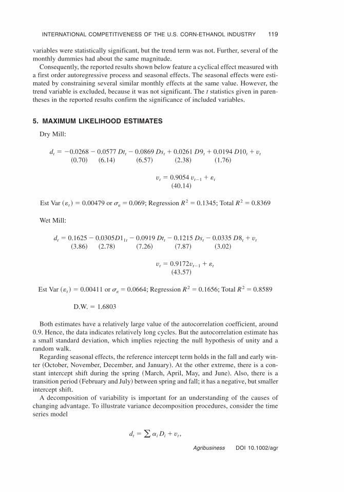
Consequently, the reported results shown below feature a cyclical effect measured witha first order autoregressive process and seasonal effects+ The seasonal effects were esti-mated by constraining several similar monthly effects at the same value+ However, thetrend variable is excluded, because it was not significant+ The t statistics given in paren-theses in the reported results confirm the significance of included variables+

5. MAXIMUM LIKELIHOOD ESTIMATES

Dry Mill:

dt � �0+0268 � 0+0577 Dtt � 0+0869 Dst � 0+0261 D9t � 0+0194 D10t � vt~0+70! ~6+14! ~6+57! ~2+38! ~1+76!

vt � 0+9054 vt�1 � «t

~40+14!

Est Var ~«t ! � 0+00479 or s«� 0+069; Regression R2 � 0+1345; Total R2 � 0+8369

Wet Mill:

dt � 0+1625 � 0+0305D11t � 0+0919 Dtt � 0+1215 Dst � 0+0335 D8t � vt~3+86! ~2+78! ~7+26! ~7+87! ~3+02!

vt � 0+9172vt�1 � «t

~43+57!

Est Var ~«t ! � 0+00411 or s«� 0+0664; Regression R2 � 0+1656; Total R2 � 0+8589

D+W+ � 1+6803

Both estimates have a relatively large value of the autocorrelation coefficient, around0+9+ Hence, the data indicates relatively long cycles+ But the autocorrelation estimate hasa small standard deviation, which implies rejecting the null hypothesis of unity and arandom walk+

Regarding seasonal effects, the reference intercept term holds in the fall and early win-ter ~October, November, December, and January!+ At the other extreme, there is a con-stant intercept shift during the spring ~March, April, May, and June!+ Also, there is atransition period ~February and July! between spring and fall; it has a negative, but smallerintercept shift+

A decomposition of variability is important for an understanding of the causes ofchanging advantage+ To illustrate variance decomposition procedures, consider the timeseries model

dt �(ai Di � vt ,



where Di is the seasonal intercept; «t is a disturbance term with zero mean and constantvariance s2+

vt � rvt�1 � «t

Using successive backward substitutions ~Greene, 2000, p+ 532!,

vt � «t � r«t�1 � r2«t�2 � —— � rn«t�n � —,

so E~vt !� 0 and Var~vt !� E @vt2 #� s20~1 � r2 !+Consequently, the unconditional mean of the dependent variable is

E~dt ! �(ai Di and

sd2 � E @dt � E~dt !#

2 � E @vt2 #�

s 2

1 � r2+

Now, consider the variance decomposition calculations, using the regression estimatesand sample statistics+ First, [sd

2 is measured, the sample variance of the calculated valuesof d shown in Figures 1 and 2+ Next, the estimate of [s2 comes from the residuals of thetime series0regression model+ Further, we interpret E @vt2 # as including current periodrandom shocks and cumulative cyclical effects+ So the variation attributable to the cyclesubtracts variance associated with the current shock:

cycle �s 2

1 � r2� s 2+

Finally, the variation is attributed to seasonal and sampling variation is obtained as totalvariation less cyclical variation less random variation+

Overall, the time-series results suggest that random, seasonal, and cyclical factors allinfluence the cost advantage for ethanol processing from corn+ Using the time series esti-mates, the variation in the competitiveness indicator is classified in Table 1+ The esti-mates suggest that about 15% of the variation is caused by current year shocks in thecommodity and financial markets+ About 75% of the variation is periodic in nature, so

TABLE 1+ Sources of Variation in the CompetitivenessIndicator

Dry Mill Wet Mill

Random 15+9 13+3Cyclical 72+4 70+6Other ~Seasonal! 11+8 16+1Total 100+0 100+0

Note. In % ~00100!+



that several years of favorable or unfavorable competition outcomes may occur+ Finally,seasonal factors account for 10–15% of the variation+

6. PROFITABILITY COMPARISONS

The sample mean of d ~Table 2! indicates the long-term profit increase associated withcorn processing instead of sugar processing and importing in the absence of the ethanoltariff+ For instance, average profit would be $+1040gallon higher with a wet mill than asugar mill+Also, profits would be �$+0050gal lower with dry mills instead of sugar mills+However, neither mean appears significantly different from zero in a simple t test becausemeans are considerably less than standard deviations+

In comparing the long-run profitability of alternative processing technologies, someallowances for differential capital costs should be taken into account+ First, sugar pro-cessing and wet milling should be on about equal footing in regards to capital expenditurefor energy processing because similar steam and electricity technologies are required forbagasse and coal+ However, only the wet mill requires separation equipment for the threebyproducts+ Dry mills typically have neither a power plant nor separation equipment+

When looking at the profit difference in the wet mill0sugar comparison then, the cornadvantage should be adjusted downward by the annual capital cost associated with sep-aration equipment+We estimate this increment at about $+040gallon per year+3 Hence, thewet-mill advantage over a sugar mill reduces to about $+060gal after taking capital costdifferences into account+

When looking at the profit decrease in the dry-mill0sugar comparison, the corn advan-tage should be adjusted upward by annual capital cost increments for a power plant neededby sugar processors+ Estimates of $0+030gallon to $+150gallon should be added to thevalues of d shown in Figure 1+ The larger estimate refers to the annual gross capital costassociated with power and steam generation in a Brazilian sugar-processing plant+ The

3We developed the annual capital cost associated with separation equipment as follows+ Representativesfrom an equipment supplier informed us that the minimum practical scale for a wet mill is about 80 milliongallons+At this capacity level, the equipment associated with converting a dry mill to a wet mill would accountfor a 30% increase in the dry mill’s cost+ Separately, we had an estimate for the capital cost of a dry mill of$1+10gal+ Hence, the separation equipment will cost approximately $0+330gal � 0+3 { $1+10gal+ Next, the life ofcapital equipment is about 15 years+At 10%, interest a mortgage that repays the principle and interest over thelife of the loan is $0+13 per dollar of debt+ Finally, the annual capital cost associated with the separation equip-ment is the product of the capital cost for the separation equipment times the annual payment rate for a dollarof debt+ $0+0430gallon � 0+33 { 0+13+

TABLE 2+ Summary Statistics for the CompetitivenessIndicator, dt

January, 1973 to May, 2002

Mean SD

Wet Mill 0+1043 0+1756Dry Mill �0+0053 0+1735

Note. In $0gallon ethanol+



smaller estimate refers to the annual net capital cost when resale of surplus electricity inBrazil is possible+4

Finally, differences in non-energy operating costs point to a slight downward adjust-ment in corn’s profit advantage+We looked at the difference between ethanol processingcosts in autonomous plants of the center0south region of Brazil and dry mills of the Mid-western U+S+, using surveys from 1985, 2002, and survey adjustments based on adoptionschedules for new processing technologies+ Estimates of the cost differential are shown inTable 3+ The processing cost disadvantage for U+S+ processors was $0+0250gallon for the1980s+ But presently, it is likely around $0+0110gallon+ The difference probably narrowedbecause of cost reductions in enzymes specific to corn processing+Also, the automation-induced reduction in labor requirements possibly had a larger impact on the higher U+S+wages+ Hence, there is a slight downward adjustment to the mean value of d in Table 2because of non-energy operating costs+

4A recent survey gives capital expenditure and capacity data for several new 40 million gallon dry-millethanol plants that are under construction ~Bryan, 2004!+ Three of these are Midwestern plants using conven-tional natural gas heat and electricity plants+ One of the plants is a coal-fired dry mill in Pennsylvania+ Theadditional capital cost for the coal-fired plant is $1+20gal+ Similarly, the total capital outlay for the biomasspower plant of Table 5 comes to $1+40gal without an allowance for the capital cost of natural gas systems+ Usinga 15-year life and 10% mortgage rate gives an annual cost increment for a coal-fired dry mill of $0+1560gallon � 1+2 { 0+132+

For a lower-limit estimate, assume that an opportunity for surplus electricity sales exists+ Again, using thecase detailed in Table 5, annual electricity revenues would be

$0+1310gal � $5+256 mil040 mil gal+

Then, the net capital cost would be $+030gal � $0+1560gal � $0+1310gal+

TABLE 3+ Nonenergy Operating ~Distilling! Cost Comparisons for the United Statesand Brazil

Mid-1980’s Cost Estimates 2002 Cost Estimates

U+S+aSmall0MidsizePlants

Brazilb

Center0South

AutonomousPlants

Brazil0U+S+

Difference

U+S+cLargeDry

Mills

Brazild

Center0South

AutonomousPlants

Brazil0U+S+

Difference

____________________________ in $0gallon ____________________________

Category:Ingredients 0+0830 0+1034Labor0maintainence 0+1860 0+0952Management,

Tax, Insurance 0+0510 0+0380

Total 0+3240 0+2990e �$0+0250 0+2351 0+2243f �$0+0108

aFrom “Economics of Ethanol Production in the United States” ~AER-607! by S+ Kane and J+ Reilly, 1989, Washington, DC:U+S+ Department of Agriculture, Economic Research Service+bFrom “Subsidtos para fixacao dos precos da cana-de-asucar, do asucar e do alcool, safra 198501986” by the Fundacao GetulioVargas ~FGV!, 1985, Brazil: FGV0IAA+cFrom “The 2002 Ethanol Costs of Production Survey” ~AER! by H+ Shapouri and P+ Gallagher, 2005,Washington, DC: U+S+Department of Agriculture, Office of Energy Policy and New Uses+d25% Reduction in “b+” Cost forecast suggested in “The Brazilian National Alcohol Programme:An Economic Reappraisal andAdjustments” by R+S+ da Matta and L+ da Rocha Ferreira, 1988, Energy Economics, p+ 251+eLiters to gallons, Using 3+785 L0gal+



7. STRATEGIES FOR IMPROVING THE COMPETITIVENESSOF THE DRY-MILL INDUSTRY

There have been two episodes of investment in the U+S+ ethanol industry+ The most fun-damental cause of both episodes was likely a surge in energy markets and a spike inethanol prices+ However, byproduct prices were considerably more attractive during thefirst expansion episode in the early 1980s, at least partly because corn byproducts enteredEurope without duty, while a high import tariff was charged on corn imports+ Byproductprices have been considerably lower during the capacity expansion of the last 3 years~Figure 4!+ Consequently, investments have favored smaller dry mills without separationequipment in the recent expansion+

In this section,we consider plausible changes in dry mill management that have a poten-tial to reduce production costs+ First, the possibility of using high-starch corn is dis-cussed+ Second, the benefits and costs of biomass power generation are considered+

7.1 Corn Composition

Consider how the corn-processor’s profit function depends on process yields+ In the mostelementary form, profits are revenues from ethanol and distillers’ grain sales less expen-diture on corn and other inputs+

p � Pet Qet � Pdt Qdt � Pct Qct �( wit Xit

Equivalently, the profit function can be written in terms of prices, yields, and operatingexpenses per input unit:

p � �Pet � �Cct

Yct

� Pdt Ycd �( wit Xit

Qct

� 1

Yce�Qet

Figure 4 Distillers’ Grains Price Trend



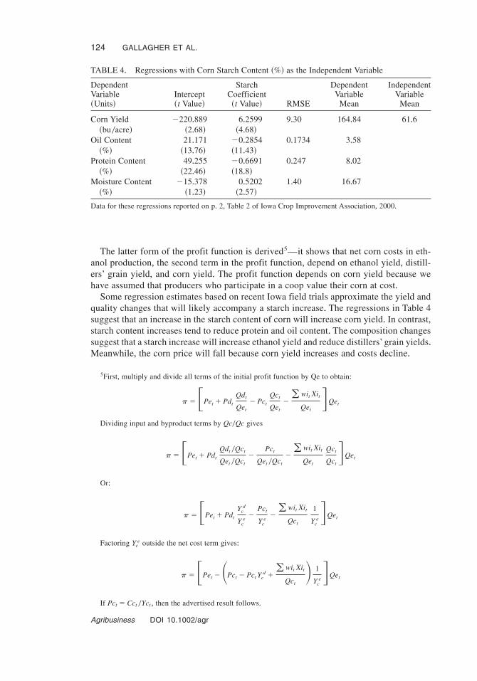
The latter form of the profit function is derived5—it shows that net corn costs in eth-anol production, the second term in the profit function, depend on ethanol yield, distill-ers’ grain yield, and corn yield+ The profit function depends on corn yield because wehave assumed that producers who participate in a coop value their corn at cost+

Some regression estimates based on recent Iowa field trials approximate the yield andquality changes that will likely accompany a starch increase+ The regressions in Table 4suggest that an increase in the starch content of corn will increase corn yield+ In contrast,starch content increases tend to reduce protein and oil content+ The composition changessuggest that a starch increase will increase ethanol yield and reduce distillers’ grain yields+Meanwhile, the corn price will fall because corn yield increases and costs decline+

5First, multiply and divide all terms of the initial profit function by Qe to obtain:

p ��Pet � Pdt

Qdt

Qet

� Pct

Qct

Qet

�( wit Xit

Qet

�Qet

Dividing input and byproduct terms by Qc0Qc gives

p ��Pet � Pdt

Qdt 0Qct

Qet 0Qct

�Pct

Qet 0Qct

�( wit Xit

Qet

Qct

Qct

�Qet

Or:

p ��Pet � Pdt

Ycd

Yce

�Pct

Yce

�( wit Xit

Qct

1

Yce�Qet

Factoring Yce outside the net cost term gives:

p ��Pet ��Pct � Pct Ycd �( wit Xit

Qct

� 1

Yce�Qet

If Pct � Cct 0Yct , then the advertised result follows+

TABLE 4+ Regressions with Corn Starch Content ~%! as the Independent Variable

DependentVariable~Units!

Intercept~t Value!

StarchCoefficient~t Value! RMSE

DependentVariable

Mean

IndependentVariable

Mean

Corn Yield �220+889 6+2599 9+30 164+84 61+6~bu0acre! ~2+68! ~4+68!

Oil Content 21+171 �0+2854 0+1734 3+58~%! ~13+76! ~11+43!

Protein Content 49+255 �0+6691 0+247 8+02~%! ~22+46! ~18+8!

Moisture Content �15+378 0+5202 1+40 16+67~%! ~1+23! ~2+57!

Data for these regressions reported on p+ 2, Table 2 of Iowa Crop Improvement Association, 2000+



Table 5 summarizes the composition, yield, and ethanol cost changes associated with a10% increase in the starch content of corn+ The regression estimates were used to approx-imate the yield and quality tradeoffs+However, composition estimates for corn were adjustedto a moisture basis of 15+5%+ To arrive at the ethanol yield, a 49+7% conversion of starchto ethanol ~by weight! was assumed, based on chemical relationships+ To arrive at distill-ers’ grain yields, the weight of 27% protein content distillers dried grain was calculatedfrom the pure protein weight; then, we verified that residual oil and fiber would be suf-ficient to fill the blending requirement+ The corn-yield estimate is based directly on theregression estimate+ The calculated cost reduction for ethanol production is calculatedusing the trend value for distillers’ grain price+ Cost savings of $+12 per gallon are obtainedfor high-starch corn+ The corn cost used for the calculations of Table 5 excludes an allow-ance for land rent, possibly referring to producers and coop members who own cropland+

To extend this analysis, the breakeven point for starch-increase profitability is givenfor a range of byproduct prices and two corn cost conditions in Figure 5+ The dotted lineshows the case where the reference corn price of $1+220bu excludes land costs+ The solidline gives the breakeven line for the reference corn price of $2+360bu when land costs areincluded+ Generally, this analysis suggests that a starch increase is a cost-reducing strat-egy, regardless of the treatment of land costs and for most distillers’ grain prices+ How-ever, the breakeven point is approached when land costs are included and when the distillersgrain price reaches 2 standard deviations above the trend line ~$1000ton!+

7.2 Biomass Power Generation

A second strategy for improving the competitiveness of dry mills is the cogeneration ofbiomass power+ Denmark’s power industry is operating six facilities that are essentiallylarge-scale demonstration projects+ Most of these plants provide electricity and district

TABLE 5+ The Effects of a 10% Increase in Corn’s StarchContenta

Proportion

Corn Composition:Content Proportion Standard High Starch

Starch +6246 +68706Protein +0815 +0536Oil +0364 +0245Fiber +1025 +07979

Yields ~units!:Corn ~bu0acre! 164+7 191+8Ethanol ~gal0bu c! 2+636 2+900Ddg ~lbs0bu c! 16+91 11+120

Ethanol Cost ~$0gal! 1+055 0+924

Assumptions:Distillers Grain Price $79+50tonCorn Cost $387+830acreaAdjusted to 15+5% moisture content+



heating for small communities+ But one plant is especially interesting because it providesthe electricity and process steam needs of a paper plant and a distiller, as well as thepower needs of a small community ~Nielsen et al+, 1998, p+38!+ The critical inputs andoutputs of the Grenaa plant are:

Power output: 18+6 MWHeat output: 60+0 MJ0sStraw input: 55,000 metric tons0yearCoal input: 40,000 metric tons0yearCapital cost: $56,000,000 ~at 7 DK per $1!

A preliminary comparison of biomass power against natural gas and market purchasesof electricity suggests that cost savings can be achieved with biomass power ~Table 6!+First, the steam power output matches the needs of a 40 million gallon ethanol plant, and12 MW of the electrical power output is a surplus+6 Revenues from electricity sales are$5+3 million if sales to local consumers are possible+ Second, expenditures for biomassare $1+4 million—our calculations use a corn-stover price that reflects farm cost, localtransport, and a producer margin under typical corn-belt conditions ~Gallagher et al+, 2003a!+Third, a comparable amount of coal input complements seasonal availability of biomass,and costs about $1+1 million annually+ Finally, an annual capital of $7+4 million results

6The electricity requirements and steam heat for a 40 million gallon ethanol plant are

5936 Kw0h

hr�

1+3 Kw0h

gal

40 106 gal

yr

1 yr

365 day

1 day

24 h '

50+9 MJ

s�

38,000 BTU

gal

40 106 gal

yr

1 MJ

947+8 BTU

1 yr

365 day

1 day

24 hr

1 h

60 min

1 min

60 sec

Figure 5 Ethanol Cost Change From a 10% Starch Increase



from a 10% mortgage on the plant with a length that corresponds to the plant’s useful lifeof 15 years+

Constructing a biomass power plant may be a cost-reducing strategy for an ethanolproducer+ The annual net expenditure for this capital equipment comes to about $+110gallon with a 40 million gallon ethanol plant+ Presently, modern dry-mill ethanol plantsare spending about $+190gallon for market purchases of electricity and natural gas+Hence,a $+080gallon cost savings may be possible with biomass0coal generation of steam andelectricity+

8. EMERGING AVENUES OF COMPETITION

Presently, ethanol occupies a niche in a quality-differentiated U+S+ gasoline market+ Eth-anol is an additive; it has some desirable attributes, such as octane and oxygen, whichimprove the automobile and environmental performance of gasoline+ Direct competitionof ethanol in the gasoline market has been limited; alcohol fuel vehicles, such as those inBrazil, have required extensive modifications of internal combustion engines+ But newflexible fuel vehicles ~FFV! can use either gasoline or E85, a mixture of 85% alcohol and15% gasoline+ The flexible fuel vehicles have a sensor that identifies fuel properties andthe car’s computer adjusts the fuel system accordingly+ A few gas stations in the Mid-western U+S+ now sell E85+ So the technology for direct alcohol–gasoline fuel substitu-tion is emerging+

TABLE 6+ Annual Costs for Power and Electricity

Category Amount Rate

AnnualRevenue~�!or cost~�!

Net Costfor

ethanole

Cogeneration of Steam and Electricity With Corn Stover0Coal:

Electricity Sales 12,000 kw0h $+050kw0h �$5,256,000a

Corn Stover 55,000 mt0year $250mtf �$1,375,000Coal 40,000 mt0year $1+220106 BTUc �$1,091,168Capital $ 56 million $0+1320yearb

per $1 debt �$7,386,400

Total: �$4,596,568 �$0+110gallon

Market Purchases of Electricity and Natural Gas:

Electricity Purchases 1+235 Kw0h0gal $+050kw0h +06Natural Gas Purchases 36,100 BTU0gal $3+5790106 BTUd +129

Total: �$0+1910gallon

a12,000 Kw0h �$0+05kw0h

�365 day

year�

24 hday

� $5,256,000

bThe annual payment for a mortgage at 10% interest and length of 15 years+c24+648 � 106 BTU0mtd1+020 BTU0cubic footeBased on a 40 million gallon ethanol plant+f15+4 � 106 BTU0mt+ The BTU price of corn stover is

$1+624106BTU

�$25mt{

mt

15+4 106 BTU



But can E85 compete with commodity gasoline directly? For an answer, we first com-pare the wholesale prices for premium-grade gasoline with production costs for E85+Wefocus on premium gasoline because E85, with an octane rating of 105, can replace pre-mium+ So premium fuel is likely the first market where alcohol fuel can compete directly+According to Figure 6, E85 has been on the margin of potential competition over the last5 years+ During several months of 2001 and 2005, wholesale prices for premium gasolinehas exceeded E85 production costs+

Our method of calculating E85 costs deserves comment+ Recent estimates of operatingcosts and capital costs for U+S+ ethanol plants are available ~Gallagher,Brubaker,& Shapouri,2005; Shapouri & Gallagher 2005!+Annual capital cost, the yearly allowance for mortgagerepayment over the life of the plant, was divided by plant capacity, and added to unit-operating costs for an estimate of total unit costs+Hence, the ethanol cost estimate includesan allowance for a normal return to capital+Next, E85 cost is a ~85%:15%!weighted aver-age of ethanol costs and the wholesale price of regular ~conventional! gasoline in Iowa+

Also, E85 costs are expressed in “dollars per gallon of gasoline equivalent+” That is, theethanol cost estimate has been adjusted to reflect the reduced fuel economy using E85 insteadof gasoline+ There is a range for the fuel economy discount+A 25% discount is typical forcars tested as they are manufactured, adjusted for primary use of gasoline ~Energy Infor-mationAdministrationAgency and U+S+Environmental ProtectionAgency, 2004, p+ 17!+Adiscount of 5% to 15% is given for flexible fuel vehicles ~FFVs! that have been optimizedfor E85 as the primary fuel ~National EthanolVehicle Coalition,2004!+We use a 15% discount

Figure 6 Wholesale Price of Premium Gasoline ~Various Grades! and E85 Breakeven Price: 2000to 2004



in our analysis,which seems appropriate for a long-run analysis+However, a short-run analy-sis looking at the ability to dispose of ethanol surpluses,which omits capital costs and usesa fuel economy 25% discount, would give about the same cost estimate+

Another question is “At what price can ethanol compete with petroleum as a commod-ity fuel?” An answer to this question requires two steps+ First, we regress for a marketingmargin relationship between the petroleum price and the price of reformulated premiumgasoline+ Second, we set the E85 cost equal to the dependent variable from the wholesalegasoline price regression, and calculate the implied value for the independent variable,the petroleum price+

The marketing margin regression gives the wholesale price of premium-grade refor-mulated gasoline as the independent variable+ The main independent variable is the priceof petroleum, which is expressed in the same ~$0gal! units as the dependent variable+Dummy variables indicate stricter environmental regulations on gasoline recipes that wentinto effect beginning in 2000, and that occur each year with summer fuel recipes+ Theregression below was estimated using monthly data from the 1995–2004 period:

Prt � 0+2136 � 0+1432D00t � 0+0895 DSUMt � 0+9565~Ppt 042!~6+4! ~5+4! ~4+9! ~6+4!

OR2 � 0+84 Ss � 0+10

The implied breakeven price ~BEP! for petroleum is calculated by setting e85 costequal to the dependent variable in the regression+ The calculated petroleum price in Fig-ure 7 is the BEP where E85 begins to compete with premium gasoline+ The BEP variessomewhat from period-to-period, with variables that affect ethanol cost and the gasoline–petroleum price relationship+ In the early 1990s, E85 was not even close to petroleum asa commodity fuel+ The BEP declined to the $350barrel range in 2000 though, with tighterrefining regulations and wider gasoline-refining margins+ The BEP briefly rose above$550bbl with springtime corn prices that rose to $3+400bushel+ But the BEP has returnedto the $400bbl range after the 2004 reduced corn prices+

This simple BEP analysis sheds some light on the ability of ethanol to compete withoutsubsidies+ Ethanol costs, which do not depend on the subsidy, are used to identify BEPs+An important competitive threshold was crossed recently, as increasing petroleum pricesand tighter environmental restrictions have intersected with relatively stable ethanol costs+However, ethanol would likely compete in the additives market with lower petroleumprices; the shadow values associated with ethanol’s quality attributes must also be included,but such an analysis is beyond the scope of this article+

9. CONCLUSIONS

The competitiveness indicator of this article measures the performance of the U+S+ corn-processing industry under a hypothetical situation that excludes the present tariffs on ethanoltrade+ First, the competitiveness measure accounts for the processing-cost effects of chang-ing conditions in commodity and foreign currency markets with today’s technology+ So,it defines the direction of trade in the event that there are no tariffs+ Second, thecompetitiveness measure can be adjusted to indicate the long-term profit advantage for acorn-processing investment relative to a sugar-processing investment, under a no-trade



barrier regime+ Hence, it is useful for accessing the relative strength of the U+S+ corn-processing industry+

A main result of the empirical investigation is that there is no trend in cost advantagetowards producing corn-ethanol in the US, or producing sugar-ethanol in Brazil and export-ing to the US+ However, there are seasonal patterns of advantage+ Further, cycles that areseveral years in length suggest periods of several years where processing costs could bereduced substantially by choosing one location or the other+ These cycles are likely causedby corresponding cycles in corn prices, sugar prices, or foreign currency prices+

According to long-term averages of the statistical competitiveness indicator, wet millsappear to have a slight advantage over sugar, while dry mills have a slight disadvantage+However, the wet-mill advantage is partly offset when the capital costs for separationequipment and a slight disadvantage for non-energy operating costs are taken into account+Similarly, the statistical average of the indicator suggests that dry mills have a slightdisadvantage relative to sugar+ But the dry-mill disadvantage is jointly offset by the cap-ital costs avoided by using natural gas for power generation and reinforced by a slightdisadvantage in non-energy operating costs+We estimate the net advantage in long-termprofits at $+050gallon for wet mills and �$+030gallon for wet mills and dry mills, respec-tively+ Hence, ethanol-processing investments might gravitate towards a corn-processingregion, such as the US, if there were no trade barriers in the ethanol market+ However, nostatistically significant difference exists for wet mills or dry mills+

For the future, the cost advantage for dry mills could be improved by changes in firm man-agement+ First, a strategy of using higher starch content in the corn could reduce ethanolproduction costs by nearly a $+120gallon+ Generally, desired quality improvements can beachieved through contracts and premiums for particular quality characteristics, but attention

Figure 7 Petroleum Prices:Actual Landed Cost of Saudi Crude ~–! and Implied Breakeven PriceBetween E85 and Premium Reformulated Gasoline



to uniformity and achievable quality targets are also important ~Wilson & Dahl,1999,p+217!+In this instance, corn processors could pay suppliers for starch content+However, the cost-reduction estimates given in this article assume a cooperative organization of ethanol pro-cessing with corn pricing at marginal costs+ Other economic organizations of processing,or oligopoly pricing of new corn seeds could reduce the cost savings+

Second, biomass power generation has the potential to reduce ethanol production costsin dry mills if high natural gas prices are sustained during the next decade+ Under currentconditions, ethanol costs are reduced by $+080gallon with biomass power because cornstover has an effective BTU-price that is much closer to coal than natural gas+ Further, aquantum leap in the energy balance and environmental benefits of corn–ethanol produc-tion could result, especially when the proportion of coal in the input mix is low+7 How-ever, cogeneration of power in larger dry mills may be a long-term strategy becauseintegration with the surrounding community’s electrical power generation may be required+

The time-series analysis of the competitiveness indicator helps predict trade flows underalternative policy regimes+ It is likely that the quota on tariff-free ethanol imports fromCaribbean countries and transshipments from Brazil will often be filled, for instance,because the sans-tariff processing costs favor sugar processors about one half of the time+Similarly, the time-series analysis also suggests that the US would often be an ethanolimporter without U+S+ or Brazil duties on ethanol imports+ Strictly speaking, though, theresults also suggest that the US could take an occasional or cyclical export position in theethanol market+

Presently, the substantial U+S+ and Brazilian tariffs on ethanol preclude direct trade ineither direction+ Both tariffs could be reduced for the mutual advantage of both countries,but Brazil may have little incentive for change as long as their re-export under the Carib-bean Basin Agreement grows+ Still, it is useful to know that the economic performance ofboth industries would be about equal if ethanol trade barriers were removed+

The United States may not emerge as a persistent ethanol exporter, however, especiallyif petroleum prices continue to increase beyond a $350bbl to $400bbl threshold in thepetroleum market+ Beyond the threshold, the alcohol-based fuel, E85, will begin to sub-stitute directly for commodity gasoline in the US on nearly a one-to-one basis+ Then,domestic ethanol consumption in the US would increase while gasoline consumption andpetroleum imports would decrease; the increasing domestic market for ethanol wouldlikely preclude ethanol exports+ Ethanol could compete directly in the commodity fuelmarket at this juncture, even without a subsidy+

APPENDIX

Variable Definitions for the Statistical Analysis (In Order of Use)

dt : sugar ~plus freight! loss corn ~plus energy! cost difference, in $0gallon ethanolCst : cost of sugar in ethanol production, in $0gallon ethanolCnt : net cost of corn in ethanol production, in $0gallon ethanolCft : cost of ethanol transport, South America to US, in $0gallon ethanol

7For sugar-ethanol production the energy balance ratio between net energy produced in ethanol over energyconsumed in the agricultural phase of production is 4+8 for Brazil’s sugar-ethanol system, which uses bagasseinstead of external energy for processing energy ~Rothman, Greenshields, & Calle, 1983, p+122!+ Similar cal-culations for the U+S+ corn ethanol industry, which uses external natural gas, are about 1+3+



Cet : cost of energy in corn ethanol production, in $0gallon ethanolPst : price of sugar in Brazil, in real0mtYs

e: yield of ethanol from sugarcane, 20+1 gal0mtEt : Brazil-U+S+ exchange rate, in $0real

Pct : price of corn in United States, in $0bu cornPft : price of gluten feed, in $0lbPmt : price of gluten meal, in $0lbPot : price of corn oil, in $0lbPdt : price of distillers’ grains, in $0lb

Yce: yield of ethanol from corn, 2+8 gal0bu

Ycf: yield of gluten feed from corn, 13+5 lb0bu

Ycm: yield of gluten meal from corn, 2+65 lb0bu

Yco: yield of corn oil from corn, 1+55 lb0bu

Ycd: yield of distillers’ grains from corn, 17+5 lb0bu

Pkt : price of coal, in $0tonPlt : price of electricity, in $0kw hPnt : price of natural gas, in $0ccf

Zck: coal input requirement for wet-mill ethanol production, 17,500 BTU0gallon

Zce: electricity input requirement for dry-mill ethanol production, 1+1 kw0h gallon

Zcn: natural gas input requirement for dry-mill ethanol production, 36,100 BTU0gallon

Dii � �1; in month i ~i � 1, in Feb; i � 2 in Mar; + + + + + + ; i � 11 in Dec!

0; otherwiseDst � D3t � D4t � D5t � D6t @Spring0Summer variable#Dtt � D2t � D7t @Transition Season variable#

Pet : price of ethanol, in $0gallonwit : price of input i feed, in $0lbQet : quantity of ethanol, in gallonsQdt : quantity of distillers’ grain, in lbsQct : quantity of corn, in buXit : quantity of input Xi, in lbs+Cct : cost of production for corn, in $0acreYct : corn yield, in bu0acre

Prt : wholesale price for reformulated gasoline in Illinois, premium grade, in $0gallonPpt : landed price of Saudi Petroleum in the US, in $0barrel

D00i � �1; when year � 2000

0; otherwise

D sumi � �1; April–to–September

0; otherwise

REFERENCES

Bryan, K+ ~2004, May!+ Proposed plant list: 2004+ Ethanol Producer Magazine, pp+ 24–35+Dornbusch, R+ ~1980!+ Open economy macro-economics+ New York: Basic Books, Inc+



da Matta, R+S+, & da Rocha Ferreira, L+ ~1988!+ The Brazilian National Alcohol Programme: Aneconomic reappraisal and adjustments+ Energy Economics, 10, 229–234+

Energy Information Administration Agency+ ~1999, January–2004, December!+ Petroleum Market-ing Monthly, U+S+ Department of Energy, various issues+

EconomicResearchService+ ~1999!+Feedyearbook+Washington,DC:U+S+DepartmentofAgriculture+Frey,D+ ~2001, June!+ Cogeneration:An on-site energy solution+ Paper presented at the 17th Annual

International Fuel Ethanol Workshop, St+ Paul, MN+Fundacao Getulio Vargas ~FGV!+ ~1985!+ Subsidtos para fixacao dos precos da cana-de-asucar, do

asucar e do alcool, safra 198501986+ @Getulio Vargas Foundation+ Subsidies for price selling forsugar cane, sugar, and alcohol, 198501986 crop year+# Rio de Janero, Brazil: FGV0IAA+

Fundacao Getulio Vargas ~FGV!–IBRE0DGD+ ~2002!+ Os dados de precos recebidos pelos produ-tores de cana de asucar+ @Getulio Vargas Foundation+Date of prices received by producer of canesugar+# Retrieved October 31, 2000, from http:00fgvdados+fgv+br

Gadomski, R+ ~2001, June!+ Impacts and future of energy costs for the ethanol industry+ Paper pre-sented at the 17th Annual International Fuel Ethanol Workshop, St+ Paul, MN+

Gallagher, P+ ~2004, November!+ The economics and rural development of bioenergy+ In Task forceon bioenergy ~Eds+!, The pros & cons of bioenergy: Pointing to the future ~Issue paper no+ 27!+Ames, IA: Council of Agricultural Science and Technology+

Gallagher, P+, Brubacker, H+,& Shapouri, H+ ~2005!+ Plant size: Capital cost relationships in the drymill ethanol industry+ Biomass and Bioenergy, 28, 565–571+

Gallagher, P+W+, Dikeman, M+, Fritz, J+,Wailes, E+, Gauthier,W+, & Shapouri, H+ ~2003a!+ Supplyand social cost estimates for biomass from crop residues in the United States+ Environmentaland Resource Economics, 24, 335–358+

Gallagher, P+W+, Shapouri,H+, Price, J+, Schamel,G+,& Brubaker,H+ ~2003b!+ Some long run effectsof growing markets and renewable fuel standards on additives markets and the U+S+ ethanolIndustry+ Journal of Policy Modeling, 25, 585– 608+

Gill, M+ ~1987!+ Corn-based ethanol: Situation and outlook+ In Feed situation and outlook report~Economic Research Service Fds-302, pp+ 30–37!+ Washington, DC: U+S+ Department ofAgriculture+

Greene,W+H+ ~2000!+ Econometric analysis+ Upper Saddle River, NJ: Prentice Hall+IFV Staff+ ~2004!+ ChevronTexaco building drying facility in Panama for Brazilian ethanol+ Inside

fuels and vehicles, 3~8!+ Retrieved April 8, 2004, from www+fuels and vehicles+comInternational Monetary Fund+ ~2002, October!+ International financial statistics+ Washington, DC:

Author+Iowa Crop Improvement Association+ ~2000, December 16!+ 2000 Iowa crop performance test-

corn, District 3@Suppl+# + Iowa Farmer Today+Kane, S+, Hrobavcak, J+, LeBlanc, M+, & Reilly, J+ ~1988!+ Ethanol: Economic and policy tradeoffs~Economic report no+ 585!+Washington,DC:U+S+Department of Agriculture, Economic ResearchService+

Kane, S+, & Reilly, J+ ~1989!+ Economics of ethanol production in the United States ~AER-607!+Washington, DC: U+S+ Department of Agriculture, Economic Research Service+

Kane, S+, Reilly, J+, LeBlanc,M+, & Hrobavcak, J+ ~1989!+ Ethanol’s role:An economic assessment+Agribusiness, 5~5!, 505–522+

Kennedy, P+L+, Harrison, R+W+, Kalaitzandonakes, N+G+, Peterson, H+C+, & Rindfuss, R+P+ ~1997!+Perspectives on evaluating competitiveness in agribusiness industries+ Agribusiness: An Inter-national Journal, 13~4!, 385–392+

Kirk, R+E+, & Othmer, D+E+ ~1980!+ Encyclopedia of Chemical Technology ~Vol+ 9, 3rd ed+!+ NewYork: Wiley+

MacDonald, T+, Yowell, G+, & McCormack,M+ ~2001!+ U+S+ ethanol industry: Production capacityoutlook ~Staff Report, P600–01–017!+ Sacramento, CA: California Energy Commission+

National Energy Policy Development Group+ ~2001!+ Reliable, affordable, and environmentallysound energy for America’s future+Washington, DC: Author+

National Ethanol Vehicle Coalation+ ~2004!+ What is the range of a flexible fuel ethanol vehicle?Retrieved December 10, 2004, from www+e85fuel+com0faqs0range+htm

Nikolaisen, L+ ~Ed+!, Nielsen, C+, Larsen, M+G+, Nielsen, V+, Zielke, U+, Kristensen, J+K+, & Chris-tensen, B+H+ ~1998!+ Straw for energy production: Technology, environment, economy+ Copen-hagen: Centre for Biomass Technology0Danish Energy Agency+



Organization of Petroleum Exporting Countries+ ~1999!+ OPEC annual statistical bulletin+ Vienna,Austria: Author+

Paturau, J+M+ ~1982!+ By-products of the sugar industry:An introduction to their industrial utiliza-tion+ Amsterdam: Elsevier+

Piccataggio, S+, & Finkelstein, M+ ~1996, June!+ Advances in biocatalyst development for conver-sion of corn fiber to ethanol+ Paper presented at the Corn Utilization Conference-VI, NationalCorn Growers Association and the National Corn Development Foundation, St+ Louis, MO+

Rothman, H+, Greenshields, R+, & Calle, F+R+ ~1983!+ The alcohol economy: Fuel ethanol and theBrazilian experience+ London: Frances Pinter+

Schmitz, T+G+, Seale, Jr+, J+L+, & Buzzanell, P+J+ ~2002!+ Brazil’s domination of the world sugarmarket+ In A+ Schmitz, T+H+ Spreen, W+A+ Messina, & C+B+ Moss ~Eds+!, Sugar and relatedsweetener markets: International perspectives+Wallingford, UK: CAB International+

Schmitz, T+G+, Schmitz,A+, & Seale, Jr+, J+L+ ~2003!+ Brazil’s ethanol program: The case of hiddensugar subsidies+ International Sugar Journal, 105, 254–265+

Schmitz, T+G+, Schmitz, A+, & Seale, Jr+, J+L+ ~2004!+ Determinants of Brazil’s ethanol sugar blendratios+ International Sugar Journal, 106, 586–596+

Shapouri, H+, & Gallagher, P+ ~2005!+ The 2002 ethanol costs of production survey ~AER-841!+Washington, DC: U+S+ Department of Agriculture, Office of Energy Policy and New Uses+

Staff+ ~2002, September 7!+ Driven to alcohol+ The Economist, pp+ 70–71+Tyers, R+, & Anderson, K+ ~1988!+ Liberalizing OECD agricultural policies in the Uruguay Round:

Effects on trade and welfare+ Journal of Agricultural Economics, 39, 197–216+U+S+Department of Energy and U+S+ Environmental Protection Agency+ ~2004!+ Fuel economy guide

for model year 2004 ~DOEEE-0283!+Retrieved December 10, 2004, from www+fueleconomy+govU+S+ International Trade Commission+ ~2003, January 1!+ Harmonized tariff schedule of the United

States ~2003 Basic Ed+!+ Retrieved May 30, 2003, from http:00dataweb+usite+gov0SCRIPTS0tariff_03000toc0html

Wilson, W+W+, & Dahl, B+L+ ~1999!+ Quality uncertainty in international grain market: Analyticaland competitive issues+ Review of Agricultural Economics 21, 209–224+

Paul W. Gallagher earned an Agricultural Economics PhD at the University of Minnesota in 1983.Currently, he is Associate Professor, Department of Economics, Iowa State University. E-mail:[email protected]

Gunter Schamel earned an Agricultural Economics PhD at Cornell University in 1995. Currently,he is Assistant Professor and Research Associate, Institute for Agricultural Economics & SocialScience, Humboldt University, Berlin. E-mail: [email protected]

Hosein Shapouri earned an Agricultural Economics PhD at Washington State University in 1978.Currently, he is a Senior Agricultural Economist, Office of Energy Policy, U.S. Dept. of Agricul-ture. E-mail: [email protected]

Heather Brubaker earned a Statistics and Economics BA at Iowa State University in 2002. Cur-rently, she is an Instructor, Department of Education, State of Iowa. E-mail: [email protected]



the international competitiveness of the u.s. corn-ethanol industry: a comparison with sugar-ethanol...

Documents