the iri seasonal climate prediction system and the …goddard/papers/mason_etal_1999.pdfthe...

1853Bulletin of the American Meteorological Society

1. Introduction: The InternationalResearch Institute for ClimatePrediction

Until fairly recently, no method was available forreliably predicting the variability of the global climatesystem on seasonal to interannual timescales.However, beginning in the mid-1960s, observationaland diagnostic studies of the ocean and atmospherebegan to make it clear that certain behaviors of thecoupled system might indeed be predictable, includ-ing in particular the El Niño–Southern Oscillation

(ENSO) phenomenon (see, among many others,Bjerknes 1966, 1969, 1972; Davis 1976; Horel andWallace 1981; Wallace and Gutzler 1981; Rasmussonand Carpenter 1982; Shukla and Wallace 1983;Philander 1983; Latif et al. 1998; Neelin et al. 1998;Stockdale et al. 1998a). In 1985, the World ClimateResearch Programme (WCRP) initiated the TropicalOceans Global Atmosphere (TOGA) program (WCRP1985). Under TOGA, increased attention was devotedto the development of physical/mathematical modelsof the ocean and atmosphere in the tropical PacificOcean, as well as to the establishment of observingsystems to provide the data such models required. AsTOGA progressed, the Tropical Atmosphere OceanArray was designed and implemented (Hayes et al.1991; McPhaden et al. 1998), and models began toshow evidence of the capability to make useful real-time predictions (Cane and Zebiak 1985; Cane et al.1986).

By 1990, research results inspired an internationalgroup of scientists to prepare a plan for the Interna-tional Research Institute for Climate Prediction (IRI).This plan outlined the scientific background justify-ing the creation of the institute as well as the benefitsto be derived from its implementation. Following the

The IRI Seasonal Climate PredictionSystem and the 1997/98

El Niño Event

Simon J. Mason,* Lisa Goddard,* Nicholas E. Graham,*Elena Yulaeva,* Liqiang Sun,* and Philip A. Arkin+

ABSTRACT

The International Research Institute for Climate Prediction (IRI) was formed in late 1996 with the aim of fosteringthe improvement, production, and use of global forecasts of seasonal to interannual climate variability for the explicitbenefit of society. The development of the 1997/98 El Niño provided an ideal impetus to the IRI Experimental ForecastDivision (IRI EFD) to generate seasonal climate forecasts on an operational basis. In the production of these forecastsan extensive suite of forecasting tools has been developed, and these are described in this paper. An argument is madefor the need for a multimodel ensemble approach and for extensive validation of each model’s ability to simulateinterannual climate variability accurately. The need for global sea surface temperature forecasts is demonstrated. Forecastsof precipitation and air temperature are presented in the form of “net assessments,” following the format adopted by theregional consensus forums. During the 1997/98 El Niño, the skill of the net assessments was greater than chance, exceptover Europe, and in most cases was an improvement over a forecast of persistence of the latest month’s climate anomaly.

*International Research Institute for Climate Prediction, ScrippsInstitution of Oceanography, University of California, San Diego,La Jolla, California.+International Research Institute for Climate Prediction, Lamont-Doherty Earth Observatory, Columbia University, Palisades, NewYork.Corresponding author address: Dr. Simon J. Mason, InternationalResearch Institute for Climate Prediction, Scripps Institution ofOceanography, University of California, San Diego, 9500 GilmanDrive, La Jolla, CA 92093-0235.E-mail: [email protected] final form 19 May 1999. 1999 American Meteorological Society

1854 Vol. 80, No. 9, September 1999

International Forum on Forecasting El Niño: Launch-ing an International Research Institute (6–8 Novem-ber 1995, Washington, D.C.), the National Oceanicand Atmospheric Administration (NOAA) committeditself to support an interim IRI, and to facilitate thetransition to a multinational institute. The IRI wasestablished in late 1996 at Lamont-Doherty EarthObservatory and Scripps Institution of Oceanography(SIO) (Carson 1998).

The mission of the IRI is to foster the improve-ment, production, and use of global forecasts of sea-sonal to interannual climate variability for the explicitbenefit of society. To accomplish this mission, the IRI,in coordination and collaboration with the interna-tional climate research and applications communities,develops and implements

• improved mathematical models of the physical cli-mate system;

• better techniques for forecasting seasonal tointerannual variations in the physical climatesystem;

• techniques for monitoring such variations, and fordisseminating climate monitoring and forecastinginformation products to potential users;

• more advanced applications of forecasts and otherclimate information products; and

• methods of training potential users of IRI productsso as to ensure the existence of a growing cadre ofenthusiastic proponents ready to apply such infor-mation to the benefit of their societies.

The IRI consists of four divisions and a trainingprogram. These include the Modeling Research Divi-sion (MRD), Experimental Forecasting Division(EFD), Climate Monitoring and Dissemination Divi-sion (CMD), and Applications Research Division(ARD). The Modeling Research Division aims to pro-vide a continually evolving suite of tools representingthe state of the art for seasonal to interannual climateprediction and forecast applications. In the near term,the MRD will focus its efforts on the development andimplementation of better models of the coupled ocean–land–atmosphere system, improving methods of oceandata assimilation, and developing methods for usingensembles of realizations from individual models aswell as from multiple models, in collaboration with theExperimental Forecast Division. The ExperimentalForecast Division, currently located at SIO, is the op-erational forecasting arm of the IRI. Its mission is toproduce regularly the most useful and accurate pos-

sible forecasts of seasonal to interannual climate vari-ability at global and regional scales. The division tookan active role in providing seasonal climate forecaststhroughout the 1997/98 El Niño episode. The ClimateMonitoring and Dissemination Division aims to pro-vide the formal distribution of IRI products, empha-sizing service to the applications community. TheCMD maintains the datasets required to permit IRIscientists to monitor current climatic conditions andconduct their research, and distributes IRI forecastsand other products, both directly to users in the Cli-mate Information Digest and via the IRI Web site. Theclimate information digest contains a synopsis of cur-rent climatic conditions, a description of the most re-cent IRI forecasts, and a summary of the impacts ofboth current and expected events on several applica-tions sectors. The aim of the Applications ResearchDivision is to maximize the utility and accessibilityof climate forecast products for societies around theworld, building on the efforts initiated by NOAA(Buizer et al. 1999). It strives to facilitate the use ofIRI forecast guidance products to improve planningand decision making in climate-sensitive sectors, andto demonstrate how climate information can enhancesustainable economic growth and reduce vulnerabil-ity to climate-related hazards including extreme eventsand disease outbreaks. The training program is an out-reach effort whose ultimate purpose is to increase theglobal awareness of the need for IRI products. It seeksto create a cadre of international experts, from a vari-ety of economic and social sectors, each of whom un-derstands and is able to make efficient application ofthe kinds of climate products that the IRI generates.

The principal purpose of this paper is to describethe developing IRI climate forecast system and itsperformance during the intense El Niño of 1997/98.This introduction is followed by an explanation of thehistorical and intellectual basis for the IRI EFD fore-cast process. The modeling methodology and the statisti-cal tools used are described in sections 3 and 4. Section5 discusses the validation of the forecast process, whilesection 6 describes the future plans for the operation.

2. Forecasting at the IRI ExperimentalForecasting Division

The IRI operational forecast system is based on thepremise that the atmospheric response to sea surfacetemperature (SST) variability provides the potential toproduce forecasts of seasonal climate anomalies for


many areas of the world (Palmer and Anderson 1994;Shukla 1998). Recent advances in understanding andmodeling of the global ocean–atmosphere system havepermitted the production of such forecasts on a regu-lar basis. A key development has been the ability dem-onstrated in the mid-1980s to forecast SSTs in theequatorial Pacific Ocean with lead times of as muchas a year (Zebiak and Cane 1987), although lead timesof about six months are now considered more realis-tic (Barnston et al. 1994, 1999a). The El Niño phenom-enon constitutes the strongest signal in the interannualvariability of global SST and exhibits major effects onclimate variability in many parts of the world(Ropelewski and Halpert 1987, 1989; Halpert andRopelewski 1992; Trenberth et al. 1998). However, itseffects in some areas are far less robust, and the cli-mate in these parts of the world may instead be affectedby SST variability in ocean basins other than the Pa-cific. Seasonal forecasts of global atmospheric anoma-lies therefore depend upon an ability to forecast SSTsin areas beyond the equatorial Pacific.

The development of the 1997/98 El Niño providedan ideal opportunity to generate seasonal climate fore-casts on an operational basis. A successful forecast ofan El Niño had first been provided in 1986 (Cane et al.1986). The 1991/92 event was again forecast success-fully, notwithstanding some false alarms that wereissued in 1990 (Mo 1993; Ropelewski et al. 1993).Forecasts of the 1997/98 event were unique, however,in that for the first time forecasts of the event, and ofseasonal atmospheric climate anomalies, were madewidely available to the general public (Barnston et al.1999b; Buizer et al. 1999). Forecasts of a strongEl Niño were available to the public as early as June1997 (Barnston et al. 1999a). The IRI EFD took anactive role in forecasting this El Niño and global cli-mate anomalies during the 1997/98 season. In thispaper, some of the tools and methods that contributedto the climate forecasts issued by the IRI EFD duringthe height of the 1997/98 El Niño are described.

3. Two-tiered dynamical modeling

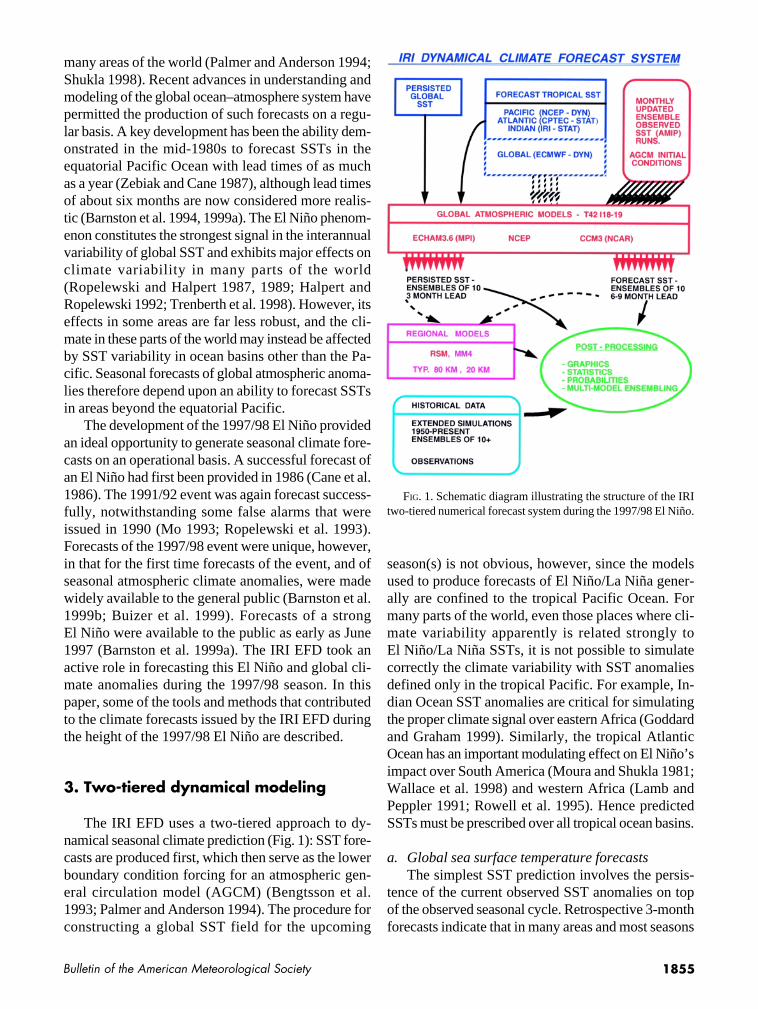
The IRI EFD uses a two-tiered approach to dy-namical seasonal climate prediction (Fig. 1): SST fore-casts are produced first, which then serve as the lowerboundary condition forcing for an atmospheric gen-eral circulation model (AGCM) (Bengtsson et al.1993; Palmer and Anderson 1994). The procedure forconstructing a global SST field for the upcoming

season(s) is not obvious, however, since the modelsused to produce forecasts of El Niño/La Niña gener-ally are confined to the tropical Pacific Ocean. Formany parts of the world, even those places where cli-mate variability apparently is related strongly toEl Niño/La Niña SSTs, it is not possible to simulatecorrectly the climate variability with SST anomaliesdefined only in the tropical Pacific. For example, In-dian Ocean SST anomalies are critical for simulatingthe proper climate signal over eastern Africa (Goddardand Graham 1999). Similarly, the tropical AtlanticOcean has an important modulating effect on El Niño’simpact over South America (Moura and Shukla 1981;Wallace et al. 1998) and western Africa (Lamb andPeppler 1991; Rowell et al. 1995). Hence predictedSSTs must be prescribed over all tropical ocean basins.

a. Global sea surface temperature forecastsThe simplest SST prediction involves the persis-

tence of the current observed SST anomalies on topof the observed seasonal cycle. Retrospective 3-monthforecasts indicate that in many areas and most seasons

FIG. 1. Schematic diagram illustrating the structure of the IRItwo-tiered numerical forecast system during the 1997/98 El Niño.


this approach to SST prediction is almost as skillfulas if one had known the true SST values for the fore-cast period. Thus persisted SST anomaly forecasts areuseful for short-term climate forecasting, particularlywhen there is no significant ENSO variability presentand the evolution of SSTs may be difficult to deter-mine. For longer lead times, and when an ENSO ex-treme of either sign is developing or decaying, suchas in 1997 and 1998, it is preferable to use a predic-tion of evolving SST anomalies.

Operational forecasts of SST anomalies for thetropical Pacific were obtained from the National Cen-ters for Environmental Prediction (NCEP) coupledmodel (Ji et al. 1998). The model Pacific, and hencethe SST forecasts, are constrained to cover the areafrom 30°N to 25°S and from 120°E to 70°W. Theocean model is initialized by assimilating observedsurface and subsurface data. The ocean model is ini-tialized by assimilating observed surface and subsur-face data. The ocean model is then coupled to theatmospheric model, and the coupled model integra-tion extends 6 months into the future. The coupledmodel uses stress, heat, and salinity flux anomaliesobtained from the coupled interaction between oceanand atmosphere models added to observed climato-logical fluxes to provide the forcing to the OGCM andAGCM. The resulting SST fields are statistically cor-rected offline.

These forecasts of SST anomalies for the tropicalPacific Ocean were supplemented by statistical fore-casts of SSTs for the Indian and Atlantic Oceans. TheIndian Ocean usually warms during El Niño and coolsduring La Niña episodes (Pan and Oort 1983; Cadet1985; Meehl 1993; Hastenrath et al. 1993; Latif et al.1994; Latif and Barnett 1995; Nagai et al. 1995;Nicholson 1997; Landman and Mason 1999), with thetropical Pacific SST anomalies leading by approxi-mately three months (Nicholson 1997; Goddard andGraham 1999). A canonical correlation analysis(CCA) model has been developed on the basis of thislagged association, relating Indian Ocean SSTs toSSTs in the tropical Pacific Ocean. This method ofpredicting Indian Ocean SST anomalies is intendedonly as an interim solution until such time as highquality global SST predictions become available fromcoupled ocean–atmosphere models. Similarly, thetropical Atlantic Ocean evolution currently is forecastusing a CCA model that was developed at Centro dePrevisão de Tempo e Estudos Climáticos (CPTEC)/Instituto Nacional de Pesquisas Espaciais (INPE) inBrazil (Pezzi et al. 1998). In the mid- and high lati-

tudes of all three oceans, observed sea surface tempera-ture anomalies were slowly damped with an e-foldingtime of 90 days.

b. Global atmospheric forecastsBecause of the requirement to provide global fore-

casts, a multimodel ensemble approach has beenadopted so that the weaknesses of one AGCM can beoffset by the strengths of another. In the initial selec-tion of AGCMs, a wide range of models was consid-ered with the aim of identifying a manageable subsetthat could be used in the production of the operationalforecasts. The criterion used was the models’ abilityto simulate observed climate variability; this skill canbe tested in a number of ways. One method used toassess the skill of the ensemble mean variability in-volves a comparison of the primary modes of observedand simulated variability. The first two empirical or-thogonal functions (EOFs) from the observed data arecalculated for various continental-scale regions, andthe model simulations are projected onto those. A cor-relation matrix is then formed between the actual (ob-served) and projected (model) EOF amplitudes todetermine how much of the dominant observed vari-ability is captured by the model. Various performancescores can be calculated to determine the percentagevariability that can be extracted from the model fieldsand has helped determine which AGCMs would bechosen for operational work.

After testing a wide range of AGCMs, the IRI EFDselected three to be used operationally: ECHAM3(Max Planck Institute), MRF9 (NCEP), and CCM3(National Center for Atmospheric Research). Whilethese three models perform approximately equallywell on average, differences in model performance forspecific variables in different regions and seasons areevident. Since the IRI EFD produces forecasts for theinternational community, it was essential that amultimodel ensemble approach be taken. All threemodels were run at T42 resolution (approximately 2.8°of latitude and longitude) with vertical resolutions of19, 18, and 18 levels, respectively, and all were forcedwith both persisted and forecast SSTs. Predictionsusing persisted SSTs were confined to 3 months be-cause of the rapid loss of skill at longer leads, but pre-dictions out to 6 months were generated using forecastSST anomalies. A comparison of scenarios based onpersisted versus evolving SST anomalies providedinformation on the sensitivity of the climate systemto the evolving boundary layer forcing and thus facili-tated the interpretation of AGCM predictions.


Each month an ensemble of at least 10 runs wascomputed for each SST scenario and each AGCM,thus providing a total ensemble size of more than 60.Debate still exists over the optimal number of en-semble members, but a compromise must be found be-tween an acceptable number and the amount ofcomputer time required to generate the ensemble. Inmost cases an ensemble of 10 appeared to be sufficientto sample the probability distribution of the seasonalclimate variability with a given AGCM and SST sce-nario. Because initialization shocks may result fromusing AGCM-based reanalysis products as initial con-ditions in alternative AGCMs, the individual en-semble members were initialized from continuallyupdated simulations using observed sea surface tem-peratures, and thus they did not include any informa-tion about the actual initial conditions of theobserved atmosphere.

4. Statistical tools

The raw output of numerical models, whether ofthe atmosphere alone or of the coupled ocean–atmosphere system, is not enough to permit a forecastto be made. The great sensitivity of the behavior of theatmosphere to small differences in initial conditionsmakes it necessary to use ensembles of many modelexecutions, but it adds a complex step in the need tointerpret the ensemble output. Statistical analyses ofthe model outputs therefore are required. In addition,at the present state of such models, statistical predic-tions from historical data can provide useful ancillaryinformation.

a. Ensemble meansEnsemble methods typically are used to indicate

the range of possible climate outcomes for a given SSTboundary forcing (Milton 1990; Murphy 1990;Mureau et al. 1993; Tracton and Kalnay 1993; Déquéet al. 1994; Harrison 1995; Anderson 1996), but meth-ods of presenting and interpreting the forecast infor-mation contained within the ensemble are not obvious.In addition, because of model errors and biases, theensemble distribution may not accurately represent thetrue distribution of possible outcomes. The IRI EFDhas adopted and developed a range of methods for dis-playing AGCM ensemble output.

The simplest form of presentation of ensemble in-formation is the ensemble mean (Fig. 2a). Maps of theensemble mean climate predictions together with in-

formation based on the historical performance of themodel are produced. A mask is applied to the model-predicted anomaly map such that the anomalies areshaded only in regions where the model skill, as mea-sured by the correlation between the ensemble meananomaly and the observed anomaly, is statistically sig-nificant (Fig. 2b). For the temperature predictions, theanomaly fields are plotted; for the precipitation, theanomalies are expressed as an absolute quantity(mm day−1) (Fig. 3) and as a relative quantity (% nor-mal, where 100% normal implies no anomaly)(Fig. 4).

The correlation mask indicates where the modelsimulates the observed climate variability reasonablywell. Because the correlation coefficient is an imper-fect measure of model performance (Potts et al. 1996),the correlation mask may hide the output in someplaces where there is some model skill. In other places,

FIG. 2. (a) Ensemble mean prediction of January–March 1998air temperature anomalies (°C) relative to a 1961–90 climatology.The prediction was produced in December 1997 and consists of10 ensemble members from the CCM3 model forced with fore-cast tropical Pacific and Indian Ocean SSTs, with persisted anoma-lies elsewhere. In (b) the temperature anomalies are masked wherethe correlation between simulated and observed variability doesnot exceed the 90% confidence level for this season over the years1950–94.


systematic model biases may result in poor correla-tions with observed climate variability, but simple cor-rections to the model output may provide some usefulinformation. One approach to capturing this informa-tion is to compile “ensemble mean contingencytables,” thus comparing the historical performance ofthe model to the observations according to tercile clas-sifications rather than by some form of squared errorstatistic, such as the correlation coefficient. The cli-

mate anomalies are classified such that, in the case ofprecipitation (temperature), the wettest (warmest) thirdof the values is defined as “above normal,” the middlethird is “near normal,” and the driest (coldest) third is“below normal.” The contingency table is built bycounting how often the observed anomaly was above,near, or below normal given the predicted category.A table is built for each grid point for the season un-der consideration, and the information is displayed as

FIG. 3. (a) Ensemble mean prediction of September–Novem-ber 1997 anomalous precipitation rates (mm day−1) relative to a1961–90 climatology. The prediction was produced in Septem-ber 1997 and consists of 10 ensemble members from theECHAM3 model forced with forecast SST anomalies for the tropi-cal Pacific and Indian Oceans, and persisted anomalies elsewhere.In (b) the anomalous precipitation rates are masked where thecorrelation between simulated and observed variability does notexceed the 90% confidence level for this season over the years1950–94.

FIG. 4. (a) Ensemble mean prediction of September–Novem-ber 1997 anomalous precipitation as a percentage of average sea-sonal rainfall relative to a 1961–90 climatology. The predictionwas produced in September 1997 and consists of 10 ensemblemembers from the ECHAM3 model forced with forecast SSTanomalies for the tropical Pacific and Indian Oceans, and persistedanomalies elsewhere. In (b) the anomalous precipitation is maskedwhere the correlation between simulated and observed variabil-ity does not exceed the 90% confidence level for this season overthe years 1950–94.


four maps (Fig. 5). The firstshows the spatial probabilitiesassociated with an above-normalprediction (Fig. 5a), the secondshows the probabilities of nearnormal (Fig. 5b), the third showsthe probabilities of below nor-mal (Fig. 5c), and the fourth is arebuilt forecast (Fig. 5d). Therebuilt forecast highlights a cat-egory that has been assigneda probability of at least 50%.For those points for which twoneighboring categories are ap-proximately equally likely, andthe third has been assigned aprobability of less than 30%,then the rebuilt forecast indi-cates the improbability of the“unlikely category.” Followingthis logic, the rebuilt forecastconsists of five categories: “dry,”“not wet,” “near normal,” “notdry,” and “wet,” in the case ofprecipitation.

b. Estimation of forecastprobabilitiesIn addition to displaying the

ensemble mean predictions andforecast probabilities estimatedfrom the ensemble mean, sev-eral methods for extracting anddisplaying the information con-tained in the distribution of theensemble members are used.Although it can be demonstratedthat the ensemble mean pro-vides a more skillful forecast than an individual en-semble member, there can be additional importantinformation in the ensemble spread. For a number ofpredefined regions, the distribution of the ensemblemembers, the ensemble mean, and the observationalanomaly are plotted for each year (Fig. 6a). The plotindicates the year-to-year variability in the spread ofthe ensemble members, how that spread may be re-lated to the accuracy of the prediction, and whetherthe model has performed better for positive or nega-tive anomalies. In addition, the role of extreme en-semble members and the appearance of bimodaldistributions can be investigated from the plot. The

historical distribution of the ensemble members isthen used to construct a climatological probability dis-tribution function/curve for the region, against whichthe distribution of the current ensemble of predictionsfrom the same model can be compared (Fig. 6b). Aclimate signal in the regional prediction should appearas a discernable shift of the forecast distribution rela-tive to the climatological distribution.

Another simple approach for calculating and rep-resenting forecast probabilities is to calculate the per-centages of ensemble members with positive ornegative anomalies, or that fall within the upper,middle, and lower terciles. Maps showing the percent-

FIG. 5. Probability that the precipitation will fall into the (a) above-normal, (b) near-nor-mal, or (c) below-normal tercile, given the current ensemble mean forecast shown in Figs.2 and 3 and the previous behavior of the AGCM’s ensemble mean climate response; (d) a“rebuilt” forecast based on the category shown in (a)–(c) that has the greatest probability.Full details of how the rebuilt forecast is made are provided in the text.


ages of ensemble members simulating temperature andrainfall anomalies in each tercile are produced by theIRI EFD for each AGCM and sea surface temperaturescenario. Similar maps are produced indicating thepercentage of ensemble members in the upper andlower 15th percentiles. An example is provided inFig. 7, showing the ECHAM3 prediction for Africa forSeptember–November 1997 from August 1997, usingpersisted SST anomalies. The model indicated highprobabilities of extremely wet conditions over muchof eastern Africa. In some areas in the region over500% of the long-term average rainfall for September–November was received.

While it can be demonstrated that even when theprobabilities are unreliable, such probabilistic forecastinformation is of potentially greater value to decisionmakers than deterministic forecasts (Thompson 1962;Murphy 1977; Krzysztofowicz 1983), clearly it is pref-erable for the forecast probabilities to correspond withthe observed relative frequency of the forecast eventas closely as possible (Murphy and Winkler 1987).Some adjustment for reliability is therefore made tothe ensemble percentages based on the capture rates

of the ensembles. The adjust-ments are usually small and donot fully correct for model bi-ases to the same extent as thecontingency table–based ap-proach described above.

c. Statistical inflation ofensemble sizeGiven that model ensembles

are used to estimate the prob-ability distribution of possibleclimate outcomes, the model’sresponse to boundary forcingshould sample the observeddistribution as accurately andwith as much resolution as pos-sible. Larger ensembles providegreater resolution in definingthe shape of the probability dis-tribution (Buizza et al. 1998),but considerable computer re-sources are required to producelarge ensemble sizes. A simple,computationally efficient, non-parametric statistical approachfor inflating ensemble sizes hasbeen developed (Graham et al.

1999, manuscript submitted to Mon. Wea. Rev.). Thismethod, known as ensemble likelihood values frominferred statistics, is based upon the assumption that,apart from the influence of the SST boundary condi-tions, monthly values within any individual ensemblemember are independent. The assumption, if valid,permits seasonal values to be calculated by combin-ing monthly values from different ensemble members.This method of inflating the ensemble size appears toprovide a notable improvement in forecast skill inareas where there is a high degree of ensemble scat-ter and positive model skill.

d. ENSO-related climateprobabilitiesThe studies of Ropelewski and Halpert (1987, 1989)

and Halpert and Ropelewski (1992) provide a guide tothe expected climatic impacts of ENSO extremes (i.e.,El Niño and La Niña). Simply knowing that an ENSOepisode is under way appears to be sufficient to makea forecast that would improve upon one predicting thatconditions would be the same as the average for thattime of year over the past decade or two (such a forecast

FIG. 6. (a) Historical performance of the ECHAM3 model for the August–October sea-son compared to observations averaged over the “Indonesia” region (10°S–20°N, 95°–140°E). The open blue circles show the model anomaly for individual ensemble members(expressed as a percentage of long-term mean), solid blue circles show the ensemble mean,and red crosses indicate the observed anomaly. The green circles are for the current fore-cast, and the solid green circle represents the ensemble mean. The gray-shaded area indi-cates the range of the near-normal tercile based on the climatological period 1961–90. Thenumbers at the top of the graph indicate the correlation between the ensemble mean simu-lation and the observed anomalies (R) and the tercile hit score (P). (b) Distribution of fore-cast members for August–October 1997 (open green bars) relative to the climatologicaldistribution (solid blue bars).


is referred to as climatology).The IRI forecast process useshistorical manifestations ofENSO extremes as a guide tocheck and improve upon themodel results.

The historical impacts of ElNiño and La Niña events onrainfall anomalies can be illus-trated effectively by calculatingthe observed percentage of timesthat seasonal rainfall has been inthe upper, middle, and lowerclimatological terciles duringENSO extremes. Three-monthmean NIÑO3 indices were cal-culated using the Kaplan et al.(1998) sea surface temperaturedata, and the warmest 10 epi-sodes since 1950 were identifiedfor each season. The number oftimes that the observed precipi-tation and temperature anoma-lies during these warm extremeswere in each tercile were calcu-lated for each grid point andwere expressed as relative fre-quencies (Fig. 8). These valuesgive some indication of the like-lihood of observing a climateanomaly in each of the categories during strongEl Niño or La Niña years. The significance of the dif-ference between the calculated percentages and thoseexpected by chance can be calculated using the hyper-geometric theorem, or by permutation methods.

e. Analog yearsThe value of using ENSO conditions in general as

a guide to likely climate anomalies is limited. ENSOepisodes vary in strength and configuration, and someconsideration must be given to these variations. Giventhe extreme nature of the 1997/98 sea surface tempera-ture anomalies in the equatorial Pacific and tropicalIndian Oceans, the atmospheric response to the glo-bal boundary layer almost inevitably would be domi-nated by the Indo–Pacific forcing. Therefore somesimilarities to the 1982/83 El Niño, which was of anapproximate equal strength (peak NIÑO3.4 andmonthly Southern Oscillation index anomalies actu-ally exceed those in 1997/98), could be expected.Maps of 3-month climate anomalies during 1982/83

were produced, to highlight areas with marked climateanomalies, which would possibly suggest strong cli-mate responses to major ENSO episodes. The AGCMpredictions for 1997/98 were compared with those for1982/83 to help indicate systematic model biases. Asan example, a systematic northeastward shift of a bandof anomalously wet conditions over central southeast-ern South America was found to occur (Fig. 9), andso forecasts were adjusted accordingly.

f. ProcessThe various model predictions that are generated

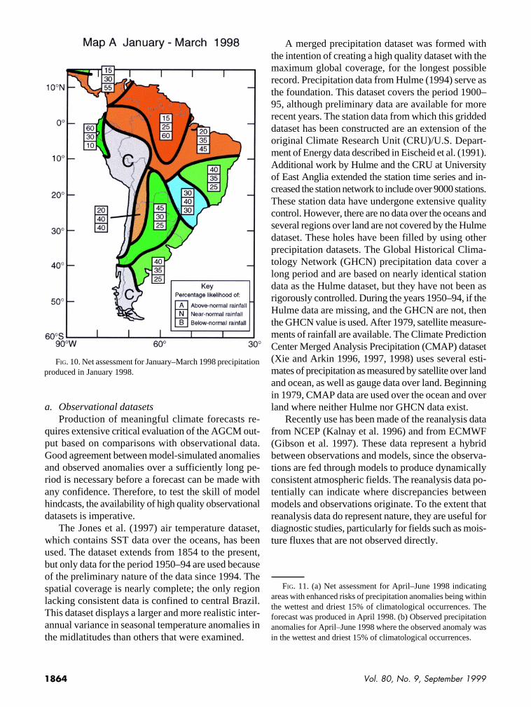
each month by the IRI EFD are not released to thegeneral public. Instead the model predictions and sta-tistical inputs are combined in a subjective manner toproduce a “net assessment,” an example of which isillustrated in Fig. 10. Inputs from external sources suchas the European Centre for Medium-Range WeatherForecasts (ECMWF), national weather services (e.g.,Barnston et al. 1999b), and the various regional con-sensus climate outlooks are considered when available.

FIG. 7. Percentages of ECHAM3 ensemble member predictions for September–November1997 in the extreme 15th percentiles. The predictions were produced in August 1997 usingpersisted sea surface temperature anomalies.


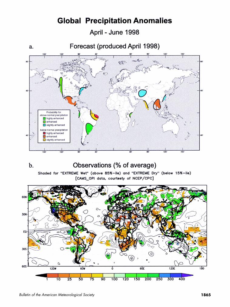
The respective value of all available information isassessed using available skill measurements, and abest-estimate forecast is provided in the net assess-ments. The net assessment forecasts are expressed interms of probabilities of the respective season’s rain-fall (temperature) being in the wettest (warmest) third,in the driest (coldest) third of years, and in the thirdcentered upon the climatological median. Indicationsof inflated risk of precipitation anomalies being in theextreme 15th percentiles have been provided sinceApril 1998. The April–June 1998 first risk of extremesmap is indicated in Fig. 11a. The extreme forecasts,including those for April–June 1998, have consistentlyshown a strong tendency to underforecast, such thatwarnings were not provided for many extreme events

that did occur. Nevertheless, thehit rate of the forecasts has beenhigh (Fig. 11b).

The production of the netassessments follows a proce-dure that is somewhat similar tothat used in the regional consen-sus forecast forums. Outputfrom these regional forums con-stitutes an important input to theIRI net assessments. Whereavailable, regions are delimitedusing boundaries that have beendefined by regional experts us-ing various statistical methods,including EOFs and clusteranalysis. The results are largelyunpublished, but in many cases,most notably in Africa, the re-gions have been defined at pre-forum workshops. In areas suchas southern Africa, the samepredefined regions are used ateach consensus meeting butmay be combined in varyingways into larger areas whereforecasts for the current seasonare identical. Where regionalexpertise is unavailable, the re-gions used in the net assess-ments are defined at the IRI onthe basis of model skill and fore-cast signal, as well as an objec-tive analysis of interannualvariability based on knownSST-related climate patterns.

The forecast regions are defined by subjectively de-limiting areas where there is some skill in at least oneof the models, and where there is an indication of aspatially coherent signal in the current modelpredictions.

Once a region has been subjectively delimited, orprovided by regional expertise, estimates of the fore-cast probabilities are made. Probabilities provided bythe regional forecast forums are revised if the net as-sessment is for a slightly different period or if newpredictions have become available since the regionalconsensus was reached. Where no regional guidanceis provided, the probabilities are estimated from thefollowing considerations: the level of agreement be-tween different dynamical and statistical model pre-

FIG. 8. Frequency of occurrence of (a) above-normal, (b) near-normal, and (c) below-normal January–March precipitation during the 10 strongest El Niño episodes since 1950(as measured by the average SST anomaly within NIÑO3.4: 5°S–5°N, 120°–170°W).


dictions, the strength of the sig-nal in the various predictions,the respective skill levels of themodels, and subjective confi-dence in the different predic-tions, based on confidence in thevarious SST forecasts used toforce the AGCMs, for example.

Clearly there is considerablescope for automating and reduc-ing the subjective componentinvolved in defining the forecastregions and estimating the fore-cast probabilities. Work is inprogress to combine the variousmodel predictions objectively,using information about histori-cal performance, and to providemodel output for predefined re-gions rather than model gridpoints, possibly including someform of statistical correction. Inthe meantime, operational re-quirements necessitate the largesubjective element involved inthe production of the net assess-ments. The operational produc-tion of the forecasts therefore isan evolving process as new toolsare gradually developed; theprocess did not remain constantthrough the 1997/98 episode.Sea surface temperature sce-narios used to force the AGCMshave developed from tropicalPacific-only forecasts in theearly stages of the El Niño, toglobal tropical sea surface tem-peratures that are used currently.Postprocessing tools have beendeveloped on an ongoing basis, and a growing list ofexternally produced forecasts and comments has beenconsidered in the production of the net assessments.

5. Forecast validation

Because of systematic errors in the models used,it is essential that estimates of confidence in the modelpredictions be made. Such estimates provide the fore-caster with indications of strengths and weaknesses in

the various models, and assist in the subjective com-bination of the model outputs and statistical productsinto the net assessment forecasts. Many of the statis-tical methods used to validate the models are used toverify the forecasts produced operationally. Forecastverification is an essential process for ensuring cred-ibility for users, and for monitoring forecast reliabil-ity. Here the observational datasets used, the processesthrough which skill estimates are derived, and limitedefforts to determine the quality of forecast performanceare described.

FIG. 9. Comparison of (a) observed December–February precipitation anomalies duringthe 1982/83 El Niño with simulated anomalies by the ECHAM3 model forced with (b) ob-served SSTs, (c) observed Pacific SSTs and climatological SSTs elsewhere, and (d) fore-cast tropical Pacific SSTs and climatological SSTs elsewhere.


a. Observational datasetsProduction of meaningful climate forecasts re-

quires extensive critical evaluation of the AGCM out-put based on comparisons with observational data.Good agreement between model-simulated anomaliesand observed anomalies over a sufficiently long pe-riod is necessary before a forecast can be made withany confidence. Therefore, to test the skill of modelhindcasts, the availability of high quality observationaldatasets is imperative.

The Jones et al. (1997) air temperature dataset,which contains SST data over the oceans, has beenused. The dataset extends from 1854 to the present,but only data for the period 1950–94 are used becauseof the preliminary nature of the data since 1994. Thespatial coverage is nearly complete; the only regionlacking consistent data is confined to central Brazil.This dataset displays a larger and more realistic inter-annual variance in seasonal temperature anomalies inthe midlatitudes than others that were examined.

A merged precipitation dataset was formed withthe intention of creating a high quality dataset with themaximum global coverage, for the longest possiblerecord. Precipitation data from Hulme (1994) serve asthe foundation. This dataset covers the period 1900–95, although preliminary data are available for morerecent years. The station data from which this griddeddataset has been constructed are an extension of theoriginal Climate Research Unit (CRU)/U.S. Depart-ment of Energy data described in Eischeid et al. (1991).Additional work by Hulme and the CRU at Universityof East Anglia extended the station time series and in-creased the station network to include over 9000 stations.These station data have undergone extensive qualitycontrol. However, there are no data over the oceans andseveral regions over land are not covered by the Hulmedataset. These holes have been filled by using otherprecipitation datasets. The Global Historical Clima-tology Network (GHCN) precipitation data cover along period and are based on nearly identical stationdata as the Hulme dataset, but they have not been asrigorously controlled. During the years 1950–94, if theHulme data are missing, and the GHCN are not, thenthe GHCN value is used. After 1979, satellite measure-ments of rainfall are available. The Climate PredictionCenter Merged Analysis Precipitation (CMAP) dataset(Xie and Arkin 1996, 1997, 1998) uses several esti-mates of precipitation as measured by satellite over landand ocean, as well as gauge data over land. Beginningin 1979, CMAP data are used over the ocean and overland where neither Hulme nor GHCN data exist.

Recently use has been made of the reanalysis datafrom NCEP (Kalnay et al. 1996) and from ECMWF(Gibson et al. 1997). These data represent a hybridbetween observations and models, since the observa-tions are fed through models to produce dynamicallyconsistent atmospheric fields. The reanalysis data po-tentially can indicate where discrepancies betweenmodels and observations originate. To the extent thatreanalysis data do represent nature, they are useful fordiagnostic studies, particularly for fields such as mois-ture fluxes that are not observed directly.

FIG. 10. Net assessment for January–March 1998 precipitationproduced in January 1998.

FIG. 11. (a) Net assessment for April–June 1998 indicatingareas with enhanced risks of precipitation anomalies being withinthe wettest and driest 15% of climatological occurrences. Theforecast was produced in April 1998. (b) Observed precipitationanomalies for April–June 1998 where the observed anomaly wasin the wettest and driest 15% of climatological occurrences.


b. Long runs and retrospective forecastingIt is essential to have long enough records to de-

fine reliable estimates of the skill of AGCM simula-tions. At the same time, it is necessary to havesufficient ensemble members for each model in orderto reduce the climatic noise in the model simulations(of course it is not possible to remove the climaticnoise from the observations) and to obtain reliable es-timates of ensemble variability. In order to have con-fidence in the validation statistics, and to determinehow stable the patterns of variability are, simulationsof at least 25 years are required; longer runs are pref-erable. The limit of how far back in the past the simu-lations are useful is dependent on the quality of theSST data used to force the model and also on the qual-ity of the observational climate data against which themodel simulations are compared.

To get consistently long runs with sufficient esti-mates of ensemble variability, simulations with allthree AGCMs covering the period from 1950 to thepresent for at least 10 ensemble members have beencompleted. The ECHAM3 simulations were forcedwith the Reynolds reconstructed SST data (Reynoldsand Smith 1994) for the period 1950–96 and Reynoldsoptimally interpolated (OI) SST data (Reynolds 1988)beginning in 1997. NCEP provided a 13-member en-semble for the years 1950–94. All 13 NCEP runs wereforced with Reynolds reconstructed SSTs. Recently,runs using CCM3 were completed yielding a set of 10simulations also covering 1950–94; five of those runswere forced with Reynolds reconstructed SSTsthroughout the whole period, and five were forced withReynolds reconstructed SSTs through 1980 and OIdata beginning in 1981.

It is unfortunate that the longrun simulations of the differentatmospheric models are notforced with the same SST fields.Given the uncertainty in the ob-servational data, though, the dif-ferences in SST fields for thehistorical simulations are as-sumed small in comparison todifferences in model formula-tion. However, a small but no-ticeable improvement in modelskill is evident in the years fol-lowing the switch to the opti-mally interpolated data in theCCM3 model. How much thisdifference in skill is attributableto the quality of SST data, howmuch to the quality of the obser-vations against which the mod-els are compared, and how muchto a potential increase in predict-ability during that period is, asyet, undetermined.

Because the long run simu-lations are forced with observedSSTs, they provide estimates ofthe confidence that can be placedin the model output given per-fect SST forecasts. These Atmo-spheric Model IntercomparisonProject (AMIP) style runs givean estimate of potential predict-ability that could be achieved

FIG. 12. Correlations between observed and ensemble mean October–December precipi-tation for the (a) NCEP, (b) CCM3, and (c) ECHAM3 models. The correlations were calcu-lated using data for 1950–94.


given perfect SST forecasts. Clearly the persistent andforecast SST fields used in the operational forecastsare imperfect, and so the true confidence may be over-estimated. In order to estimate the loss of predictabil-ity incurred when using imperfect SST forecasts,retrospective forecasts using persisted SST anomalieshave been produced using the ECHAM3 model. Theseretrospective forecasts have been completed for the pe-riod 1970 to date for the December–February, March–May, June–August, and September–Novemberseasons and are validated in the same manner as thelong runs, as discussed below.

c. Model validationThe long run simulations of the AGCMs used by

the IRI EFD, and the retrospective forecast skill of theECHAM3 model, have been validated extensively.Correlations of ensemble mean simulated precipitationand air temperature with the respective observations havebeen calculated on a grid-by-grid basis using the 45 yrof long AMIP-style and 23 yr of retrospective runs(Fig. 12). Correlations for selected area averages arecalculated in addition (Fig. 6). All calculations are per-formed using 3-month average precipitation rates andtemperatures. In general, correlations for temperatureare greater than for precipitation, and they are higher forboth variables in the Tropics than they are in the mid-latitudes. However, the models do show significant skillover many regions in the midlatitudes for at least partof the year. Comparing the correlation maps of differ-ent models (Fig. 12) indicates which model(s) are mostlikely to produce a reliable forecast over a particulararea, for a particular variable in a particular season.

Similarly, relative operating characteristic (ROC)scores (Swets 1973; Mason 1982; Mason and Graham1999) for precipitation and temperature have beencalculated for all 3-month seasons. For all threeAGCMs the scores (defined as the area beneath theROC curve as plotted on linear axes) have been cal-culated using the ensemble mean, a set of 10 ensemblemembers, and statistically inflated sets of ensemblemembers (Graham et al. 1999, manuscript submittedto Mon. Wea. Rev.). Events have been defined for thelower, upper, and middle terciles, and the lower andupper 15th percentiles. As with the correlations, theROC scores have been calculated on a grid-by-gridbasis and for selected area averages. For the retrospec-tive runs, ROC scores have been calculated using thefive ensemble members available. In general, the ROCscores mirror the areas and seasons of high predictabil-ity evident from the correlation maps. However, the

ROC curves provide additional information indicat-ing the models’ biases toward accurate simulations ofwet or dry conditions. Consistently, the curves indi-cate poor predictability of near-normal conditions forboth precipitation and temperature in all areas and allseasons. In some cases, the models appear to be ableto simulate accurately above- but not below-normalconditions, or vice versa. As an example, both theECHAM3 and NCEP models have higher skill insimulating wet, rather than dry, conditions of theSeptember–November eastern African rains (Masonand Graham 1999). In some cases, the ROC curve isable to indicate predictability not evident from the en-semble mean correlations. For example, there is someindication that the ECHAM3 model is able to simu-late accurately dry conditions of the March–May east-ern African rains (Fig. 13), which are generallyconsidered difficult to predict (Mutai et al. 1998).

d. Sensitivity experimentsSensitivity experiments have been conducted to

determine the qualitative effects of SST variability in

FIG. 13. ROC curves for March–May area-averaged rainfall foreastern Africa (10°N–10°S, 30°–50°E) from 1950 to 1994. Thehit and false alarm rates were calculated using rainfall simulatedby the ECHAM3–T42 general circulation model forced with ob-served sea surface temperatures and using 10 ensemble members.Results are shown for the simulation of rainfall in the upper (blue),middle (green), and lower (red) terciles. Rates are indicated us-ing different minimum percentages of ensemble members simu-lating rainfall in the respective tercile to issue a warning, asindicated by the values along the curves. The areas, A, beneaththe curves are indicated also.


various tropical oceans. In these experiments, the SSTsin a particular ocean basin were varied, and in the otherocean areas seasonally varying climatological SSTvalues were prescribed. To date, two of these experi-ments have been completed, one for the tropical Pa-cific (20°S–20°N, 120°E–75°W) and one for theIndian Ocean (north of 40°S and west of 120°E). Theseexperiments are referred to as Pacific Ocean Global At-mosphere and Indian Ocean Global Atmosphere. Itwas found that the Indian Ocean SST anomalies arecritical for simulating the proper climate signal oversouthern and eastern Africa (Goddard and Graham1999). Rainfall variability in eastern Africa shows astrong association with the occurrence of ENSO.However, the simulation indicates that the teleconnec-tion between ENSO and rainfall in this region of Af-rica occurs through the Indian Ocean. Thus, to predictcorrectly seasonal climate anomalies over eastern Af-rica, it is necessary to predict Indian Ocean tempera-tures in addition to predicting tropical Pacific SSTs.

e. Forecast valueInitial estimates of forecast value have been made

based on the 2 × 2 contingency table estimates of fore-cast quality that form the basis of the ROC curvesdescribed above. The contingency table can be usedto calculate a set of hit and false alarm rates for a setof forecasts of predefined meteorological or climato-logical events, such as the seasonal rainfall total be-ing within the driest 10% of historical values. Thesame contingency table is used in the cost–loss modelof forecast value estimation (Murphy 1994), by defin-ing the cost of mitigation against an expected event,the mitigated loss if the event occurs, and the loss in-curred if no warning is provided. Forecast value canthen be calculated given information on event fre-quency, forecast quality, and on the costs and losses.From a set of interviews with forecast users in thesouthern African region, cost–loss tables were com-pleted for events of interest to the users. Using theECHAM3 retrospective forecasts for December–February rainfall, averaged over the area approxi-mately between 23° and 36°S, and between 15° and32°E, savings of the order of at least U.S. $10 billionto $10 trillion per year were indicated.

f. Forecast performanceNo quantitative measure of forecast performance

has been constructed as yet. One obvious difficulty inproducing such a metric is that the format of the IRIforecasts is probabilistic, as is generally the case with

climate forecasts. Thus any single forecast can hardlybe said to have any errors, since no zero probabilityterciles are forecast and so any observed value can besaid to have been allowed for. Nevertheless, the meth-ods used to validate a set of forecasts made throughtime can be applied to estimate the performance of aspecific forecast over an area. Heidke skill scores(Wilks 1995) for the precipitation net assessments pro-duced by the IRI for the 12-month period October1997–September 1998 are summarized in Tables 1 and2. The Heidke skill score treats the forecasts determin-istically and so gives a rather crude estimate of theirskill but it does provide a useful and relatively simpleestimate of skill. The net assessments are being veri-fied more comprehensively, and there are plans to re-port on the results in detail elsewhere.

In general, the skill of the net assessments for pre-cipitation during the lifetime of the 1997/98 El Niñowas highest for the Southern Hemisphere, at theshorter lead time. The net assessment forecast skill forSouth America was consistently high, while skill forEurope and Asia was low. In most cases the forecastshave been more skillful than chance, and they were asmall improvement over forecasts of persistence of thelast month’s climate anomaly and over the use of pureENSO-related climate statistics. It is expected that thequality of the net assessment forecasts will improveas the tools used in their production are developed, andthe experience of the forecasters increases.

6. Future plans

The IRI EFD operational climate forecast systemhas proven itself already to be a valuable contributionto a global community that needs to find better meansof protecting itself from variations in weather and cli-mate. In order to improve upon this performance, sev-eral means of enhancing the numerical model forecastshave been identified, and a number of these are beingimplemented. The main areas of development includean improvement in spatial resolution through down-scaling and by higher-resolution AGCMs, and theimplementation of a fully coupled ocean–atmospheremodel in the IRI EFD. In the shorter term, an agree-ment has been reached with ECMWF to validate andexperiment with the use of the SST forecasts from theirfully coupled model (Stockdale et al. 1998b). Someinitial progress in these areas is detailed here.

In an attempt to downscale the information pro-vided by the AGCMs at T42 resolution, the NCEP


nested regional spectral model (RSM) has been usedto simulate September–January rainfall variabilityover eastern Africa for the period 1970/71 to 1996/97(Sun et al. 1999, manuscript submitted to J. Geophys.Res.). The regional model has been run at a resolutionof 80 km with a very high resolution 20-km nest overKenya. There are 19 vertical layers. The nested sys-

tem has realistic vegetation and detailed topography.The outputs from the ECHAM3 atmospheric climatemodel provide the large-scale circulation forcing forthe nested system. From two numerical integrations, anensemble mean has been calculated and validated usingan observational network of over 300 rainfall stationsthroughout Kenya. The nested system captures both

Africa 14.4 −9.1 2.2 13.9 20.7 1.7 25.2 22.7 −6.0 17.8 11.4 −0.7

Asia 5.2 3.8 −8.7 −11.9 −34.3 3.3 11.3 19.8 5.7 1.5 −16.8 0.1

Australasia 39.0 45.3 1.8 36.3 50.0 37.5 11.1 6.5 −57.1 28.8 33.9 −5.9

Europe 16.5 −35.9 −17.6 −59.3 −5.1 28.1 −7.6 −24.5 16.8 −16.8 −21.8 9.1

North America 12.2 27.3 −9.4 12.1 14.1 −8.0 −4.9 29.3 −6.3 6.5 23.6 −7.9

South America 31.3 9.9 8.9 35.9 25.7 22.8 18.5 −5.2 12.2 28.6 10.1 14.6

Globe 14.5 8.9 −4.5 6.3 8.2 6.4 11.1 5.3 2.6 10.6 7.5 1.5

TABLE 1. Heidke skill scores for the 0-month lead precipitation net assessments. The scores in italic are for a forecast of persis-tence of the latest month’s climate anomaly (middle column) and for a forecast based on the frequency of occurrence of above-normal,near-normal, and below-normal precipitation during the 10 strongest El Niño episodes since 1950 (as measured by the average SSTanomaly within NIÑO3: 5°S–5°N, 90°–150°W) (third column).

OND 1997 JFM 1998 AMJ 1998 Average

Africa N/A 12.0 23.3 1.7 4.1 2.2 −6.0 8.1 12.8 −2.1

Asia N/A −7.1 −27.9 3.3 12.8 −8.7 5.7 2.9 −18.3 4.5

Australasia N/A 43.1 52.8 37.5 −15.4 −20.9 −57.1 13.9 16.0 −9.8

Europe Ν/Α −22.2 −6.2 28.1 −28.2 −20.5 16.8 −25.2 −13.4 22.5

North America N/A 9.4 11.9 −8.0 1.1 23.0 −6.3 5.3 17.5 −7.1

South America N/A 34.7 24.4 22.8 9.6 −6.2 12.2 22.2 9.1 17.5

Globe N/A 9.7 10.4 6.4 3.3 1.6 2.6 6.5 6.0 4.5

TABLE 2. Heidke skill scores for the 3-month lead precipitation net assessments. The scores in italic are for a forecast of persis-tence of the latest month’s climate anomaly (middle column) and for a forecast based on the frequency of occurrence of above-nor-mal, near-normal, and below-normal precipitation during the 10 strongest El Niño episodes since 1950 (as measured by the averageSST anomaly within NIÑO3: 5°S–5°N, 90°–150°W) (third column).

OND 1997 JFM 1998 AMJ 1998 Average


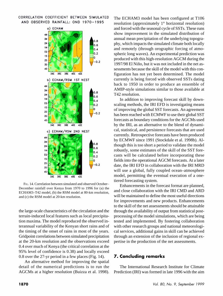
the large-scale characteristics of the circulation and theterrain-induced local features such as local precipita-tion maxima. The model reproduced the observed in-terannual variability of the Kenyan short rains and ofthe timing of the onset of rains in most of the years.Gridpoint correlations between simulated precipitationat the 20-km resolution and the observations exceed0.4 over much of Kenya (the critical correlation at the95% level of confidence is 0.38) and locally exceed0.8 over the 27-yr period in a few places (Fig. 14).

An alternative method for improving the spatialdetail of the numerical predictions is to run theAGCMs at a higher resolution (Buizza et al. 1998).

The ECHAM3 model has been configured at T106resolution (approximately 1° horizontal resolution)and forced with the seasonal cycle of SSTs. These runsshow improvement in the simulated distribution ofannual mean precipitation of the underlying topogra-phy, which impacts the simulated climate both locallyand remotely (through orographic forcing of atmo-spheric long waves). An experimental prediction wasproduced with this high-resolution AGCM during the1997/98 El Niño, but it was not included in the net as-sessments because the skill of the model with this con-figuration has not yet been determined. The modelcurrently is being forced with observed SSTs datingback to 1950 in order to produce an ensemble ofAMIP-style simulations similar to those available atT42 resolution.

In addition to improving forecast skill by down-scaling methods, the IRI EFD is investigating meansof improving the global SST forecasts. An agreementhas been reached with ECMWF to use their global SSTforecasts as boundary conditions for the AGCMs usedby the IRI, as an alternative to the blend of dynami-cal, statistical, and persistence forecasts that are usedcurrently. Retrospective forecasts have been producedby ECMWF since 1991 (Stockdale et al. 1998b). Al-though this is too short a period to validate the modelrobustly, some estimates of the skill of the SST fore-casts will be calculated before incorporating thesefields into the operational AGCM forecasts. At a laterdate, the IRI EFD in collaboration with the IRI MRDwill use a global, fully coupled ocean–atmospheremodel, permitting the eventual execution of a one-tiered forecasting system.

Enhancements in the forecast format are planned,and close collaboration with the IRI CMD and ARDwill be maintained to define the most useful directionsfor improvements and new products. Enhancementsto the skill of the net assessments should be attainablethrough the availability of output from statistical post-processing of the model simulations, which are beingtested and implemented. By fostering collaborationwith other research groups and national meteorologi-cal services, additional gains in skill can be achievedthrough an extension of the inclusion of regional ex-pertise in the production of the net assessments.

7. Concluding remarks

The International Research Institute for ClimatePrediction (IRI) was formed in late 1996 with the aim

FIG. 14. Correlation between simulated and observed October–December rainfall over Kenya from 1970 to 1996 for (a) theECHAM3–T42 model, (b) the RSM model at 80-km resolution,and (c) the RSM model at 20-km resolution.


of fostering the improvement, production, and use ofglobal forecasts of seasonal to interannual climate vari-ability for the explicit benefit of society. The devel-opment of an El Niño in early 1997, and its rapiddevelopment into a major episode, provided an idealopportunity to generate and distribute seasonal climateforecasts on an operational basis. The IRI EFD hastaken an active role in forecasting this El Niño andglobal climate anomalies during the 1997/98 seasonand has continued to produce forecast informationduring the 1998/99 La Niña.

The IRI EFD has developed a two-tiered forecastingsystem, in which forecasts of global tropical SSTs aregenerated first and then used as boundary forcing for asuite of atmospheric models. The need for forecasts ofglobal tropical SSTs has been demonstrated from expe-rience of forecasting climate variability over Africa,where the use of persisted SST anomalies can resultin incorrect climate signals in some areas. In produc-ing global climate forecasts, the IRI EFD has made useof a multimodel ensemble approach since no onemodel is able to provide accurate simulations of cli-mate variability in all regions and all seasons. All themodels used have been validated extensively to iden-tify model strengths and weaknesses, and to ensure thatit is possible to make reliable estimates of the confi-dence that can be placed in the model predictions. Inaddition to the various numerical and statistical modelsthat are run at the IRI, an effort is made to access as muchforecast information as possible from centers aroundthe world, in the production of the net assessments.

Forecasts of precipitation and air temperature arepresented in the form of “net assessments,” followingthe format adopted by the regional consensus forums,and are distributed via the World Wide Web (http://iri.ucsd.edu/forecasts/net_asmt) and with the assis-tance of the IRI Climate Monitoring and Dissemina-tion Division (IRI CMD). During the 1997/98 El Niño,the skill of the net assessments for precipitation wasgreater than chance, except over Europe, and in mostcases was an improvement over a forecast of persis-tence of the latest month’s climate anomaly and overENSO-related climate statistics. Net assessments in-dicating enhanced risk of extreme precipitationanomalies have been highly successful.

Acknowledgments. This paper was funded in part by a grant/cooperative agreement from the National Oceanic and AtmosphericAdministration (NOAA). The views expressed herein are those ofthe authors and do not necessarily reflect the views of NOAA orany of its subagencies. The computer assistance of M. Tyree, M.Olivera, J. del Corral, and N. Sheridan is gratefully acknowledged.

References

Anderson, J. L., 1996: A method for producing and evaluatingprobabilistic forecasts from ensemble model integrations. J.Climate, 9, 1518–1530.

Barnston, A. G., and Coauthors, 1994: Long-lead seasonal fore-casts—Where do we stand? Bull. Amer. Meteor. Soc., 75,2097–2114.

——, Y. He, and M. H. Glantz, 1999a: Predictive skill of statisti-cal and dynamical climate models in forecasts of SST duringthe 1997–98 El Niño episode and the 1998 La Niña onset. J.Climate, 12, 217–244.

——, and Coauthors, 1999b: NCEP forecasts for the El Niño of1997–98 and its U.S. impacts. Bull. Amer. Meteor. Soc., 80,1829–1852.

Bengtsson, L., U. Schlese, E. Roeckner, M. Latif, T. P. Barnett,and N. E. Graham, 1993: A two-tiered approach to long-rangeclimate forecasting. Science, 261, 1027–1029.

Bjerknes, J., 1966: A possible response of the atmospheric Hadleycirculation to equatorial anomalies of ocean temperature.Tellus, 18, 820–829.

——, 1969: Atmospheric teleconnections from the equatorial Pa-cific. Mon. Wea. Rev., 97, 163–172.

——, 1972: Large-scale atmospheric response to the 1964–65Pacific equatorial warming. J. Phys. Oceanogr., 2, 212–217.

Buizer, J. L., J. Foster, and D. Lund, 1999: Global impacts andregional actions: Preparing for the 1997–98 El Niño. Bull.Amer. Meteor. Soc., in press.

Buizza, R., T. Petroliagis, T. Palmer, J. Barkmeijer, M. Hamrud,A. Hollingsworth, A. Simmons, and N. Wedi, 1998: Impact ofmodel resolution and ensemble size on the performance of anEnsemble Prediction System. Quart. J. Roy. Meteor. Soc., 124,1935–1960.

Cadet, D. L., 1985: The Southern Oscillation over the IndianOcean. J. Climatol., 5, 189–212.

Cane, M. A., and S. E. Zebiak, 1985: A theory for El Niño andthe Southern Oscillation. Science, 228, 1085–1087.

——, ——, and S. C. Dolan, 1986: Experimental forecasts ofEl Niño. Nature, 321, 827–832.

Carson, D. J., 1998: Seasonal forecasting. Quart. J. Roy. Meteor.Soc., 124, 1–26.

Davis, R. E., 1976: Predictability of sea surface temperature andsea level pressure anomalies over the North Pacific Ocean. J.Phys. Oceanogr., 6, 249–266.

Déqué, M., J. F. Royer, and R. Stroe, 1994: Formulation ofGaussian probability forecasts based on model extended-rangeintegrations. Tellus, 46A, 52–65.

Eischeid, J. K., H. G. Diaz, R. S. Bradley, and P. D. Jones, 1991:A comprehensive precipitation data set for global land areas.Tech. Rep. TR051, U.S. Dept. of Energy, Carbon DioxideResearch Division, 81 pp. [Available from Climate Diagnos-tics Center, 325 Broadway, Boulder, CO 80303.]

Gibson, J. K., P. Kallberg, A. Nomura, A. Hernandez, and E.Serrano, 1997: ERA Description. ECMWF Re-Analysis ProjectReport Series, Vol. 1. [Available from ECMWF, Shinfield Park

Reading RG2 9AX, United Kingdom.]Goddard, L., and N. E. Graham, 1999: The importance of the In-

dian Ocean for simulating rainfall anomalies over eastern andsouthern Africa. J. Geophys. Res., in press.


Halpert, M. S., and C. F. Ropelewski, 1992: Surface temperaturepatterns associated with the Southern Oscillation. J. Climate,5, 577–593.

Harrison, M. S. J., 1995: Long-range seasonal forecasting since1980: Empirical and numerical prediction out to one month forthe United Kingdom. Weather, 50, 440–448.

Hastenrath, S., A. Nicklis, and L. Greischar, 1993: Atmospheric-hydrospheric mechanisms of climate anomalies in the west-ern equatorial Indian Ocean. J. Geophys. Res., 98, 20 219–20 235.

Hayes, S. P., L. J. Mangum, J. Picaut, A. Sumi, and K. Takeuchi,1991: TOGA-TOA: A moored array for real-time measure-ments in the tropical Pacific Ocean. Bull. Amer. Meteor. Soc.,72, 339–347.

Horel, J. D., and J. M. Wallace, 1981: Planetary-scale atmosphericphenomena associated with the Southern Oscillation. Mon.Wea. Rev., 109, 813–829.

Hulme, M. H., 1994: Validation of large-scale precipitation fieldsin General Circulation Models. Global Precipitation and Cli-mate Change, M. Desbois and F. Desalmund, Eds., NATO ASISeries, Springer-Verlag, 387–406.

Ji, M., A. Leetmaa, and V. E. Kousky, 1998: An improved coupledmodel for ENSO prediction and implications for ocean initial-ization. Part II: The coupled model. Mon. Wea. Rev., 126,1022–1034.

Jones, P. D., T. J. Osborn, and K. R. Briffa, 1997: Estimating sam-pling errors in large-scale temperature averages. J. Climate,10, 2548–2568.

Kalnay, E., and Coauthors, 1996: The NCEP/NCAR 40-YearReanalysis Project. Bull. Amer. Meteor. Soc., 77, 437–471.

Kaplan, A., M. A. Cane, Y. Kushnir, A. Clement, M. Blumenthal,and R. Rajagopalan, 1998: Analyses of global sea surfacetemperature 1856–1991. J. Geophys. Res., 103, 18 567–18 589.

Krzysztofowicz, R., 1983: Why should a forecaster and a deci-sion maker use Bayes theorem. Water Resour. Res., 19, 327–336.

Lamb, P. J., and R. A. Peppler, 1991: West Africa. Teleconnec-tions Linking Worldwide Climate Anomalies: Scientific Ba-sis and Societal Impact, M. H. Glantz, R. W. Katz, andN. Nicholls, Eds., Cambridge University Press, 121–189.

Landman, W. A., and S. J. Mason, 1999: Change in the associa-tion between Indian Ocean sea-surface temperatures and sum-mer rainfall over South Africa and Namibia. Int. J. Climatol.,in press.

Latif, M., and T. P. Barnett, 1995: Interactions of the tropicaloceans. J. Climate, 8, 952–964.

——, A. Sterl, M. Assenbaum, M. M. Junge, and E. Maier-Reimer,1994: Climate variability in a coupled GCM. Part II: The In-dian Ocean and monsoon. J. Climate, 7, 1449–1462.

——, and Coauthors, 1998: A review of the predictability and pre-diction of ENSO. J. Geophys. Res., 103, 14 375–14 393.

Mason, I., 1982: A model for assessment of weather forecasts.Aust. Meteor. Mag., 30, 291–303.

Mason, S. J., and N. E. Graham, 1999: Conditional probabilities,relative operating characteristics, and relative operating lev-els. Wea. Forecasting, in press.

McPhaden, M. J. and Coauthors: 1998: The Tropical Ocean–Glo-bal Atmosphere observing system: A decade of progress. J.Geophys. Res., 103, 14 169–14 240.

Meehl, G. A., 1993: A coupled air–sea biennial mechanism in thetropical Indian and Pacific regions: Role of the oceans. J. Cli-mate, 6, 31–41.

Milton, S. F., 1990: Practical extended-range forecasting usingdynamical models. Meteor. Mag., 119, 221–233.

Mo, K. C., 1993: The global climate of September–November1990: ENSO-like warming in the western Pacific and strongozone depletion over Antarctica. J. Climate, 6, 1375–1391.

Moura, A. D., and J. Shukla, 1981: On the dynamics of droughtsin northeast Brazil: Observations, theory and numerical experi-ments with a general circulation model. J. Atmos. Sci., 38,2653–2675.

Mureau, R., F. Molteni, and T. N. Palmer, 1993: Ensemble pre-diction using dynamically conditioned perturbations. Quart.J. Roy. Meteor. Soc., 119, 299–323.

Murphy, A. H., 1977: The value of climatological, categorical andprobabilistic forecasts. Mon. Wea. Rev., 105, 803–816.

——, 1994: Assessing the economic value of forecasts: An over-view of methods, results and issues. Met. Apps., 1, 69–73.

——, and R. L. Winkler, 1987: A general framework for forecastverification. Mon. Wea. Rev., 115, 1330–1338.

Murphy, J. M., 1990: Assessment of the practical utility of ex-tended range ensemble forecasts. Quart. J. Roy. Meteor. Soc.,116, 89–125.

Mutai, C. C., M. N. Ward, and A. W. Colman, 1998: Towards theprediction of the East Africa short rains based on sea-surfacetemperature–atmosphere coupling. Int. J. Climatol., 18, 975–997.

Nagai, T., Y. Kitamura, M. Endoh, and T. Tokioka, 1995: Coupledatmosphere–ocean model simulations of El Niño/SouthernOscillation with and without an active Indian Ocean. J. Cli-mate, 8, 3–14.

Neelin, J. D., D. S. Battisti, A. C. Hirst, F. F. Jin, Y. Wakata, T.Yamagata, and S. E. Zebiak, 1998: ENSO theory. J. Geophys.Res., 103, 14 261–14 290.

Nicholson, S. E., 1997: An analysis of the ENSO signal in thetropical Atlantic and western Indian Oceans. Int. J. Climatol.,17, 345–375.

Palmer, T. N., and D. L. T. Anderson, 1994: The prospects forseasonal forecasting. Quart. J. Roy. Meteor. Soc., 120, 755–793.

Pan, Y.-H., and A. H. Oort, 1983: Global climate variations con-nected with sea surface temperature anomalies in the easternequatorial Pacific Ocean for the 1958–1973 period. Mon. Wea.Rev., 111, 1244–1258.

Pezzi, L. P., C. R. Repelli, P. Nobre, I. F. A. Cavalcanti, and G.Sampaio, 1998: Forecasts of tropical Atlantic SST using a sta-tistical ocean model at CPTEC/INPE - Brazil. Exp. Long-LeadForecast Bull. Vol. 7, No.1, 28–31.

Philander, S. G. H., 1983: El Niño Southern Oscillation phenom-enon. Nature, 302, 295–301.

Potts, J. M., C. K. Folland, I. T. Jolliffe, and D. Sexton, 1996:Revised “LEPS” scores for assessing climate model simula-tions and long-range forecasts. J. Climate, 9, 34–53.

Rasmusson, E. M., and T. H. Carpenter, 1982: Variations in tropi-cal sea surface temperature and surface wind fields associatedwith the Southern Oscillation/El Niño. Mon. Wea. Rev., 110,354–384.

Reynolds, R. W., 1988: A real-time global sea surface tempera-ture analysis. J. Climate, 1, 75–86.


——, and T. M. Smith, 1994: Improved global sea surface tem-perature analysis using optimal interpolation. J. Climate, 7,929–948.

Ropelewski, C. F., and M. S. Halpert, 1987: Precipitation patternsassociated with El Niño/Southern Oscillation. Mon. Wea. Rev.,115, 1606–1626.

——, and ——, 1989: Precipitation patterns associated with thehigh index phase of the Southern Oscillation. J. Climate, 2,268–284.

——, P. J. Lamb, and D. H. Portis, 1993: The global climate forJune–August 1990: Drought returns to sub-Saharan Africa andwarm Southern Oscillation episode conditions develop in thecentral Pacific. J. Climate, 6, 2188–2212.

Rowell, D. P., C. K. Folland, K. Maskell, and M. N. Ward, 1995:Variability of summer rainfall over tropical North Africa(1906–92): Observations and modelling. Quart. J. Roy. Me-teor. Soc., 121, 669–704.

Shukla, J., 1998: Predictability in the midst of chaos: A scientificbasis for climate forecasting. Science, 282, 728–731.

——, and J. M. Wallace, 1983: Numerical simulation of the at-mospheric response to equatorial Pacific sea surface tempera-ture anomalies. J. Atmos. Sci., 40, 1613–1630.

Stockdale, T. N., A. J. Busalacchi, D. E. Harrison, and R. Seager,1998a: Ocean modeling for ENSO. J. Geophys. Res., 103,14 325–14 355.

——, D. L. T. Anderson, J. O. S. Alves, and M. A. Balmaseda,1998b: Global seasonal rainfall forecasts using a coupledocean-atmosphere model. Nature, 392, 370–373.

Swets, J. A., 1973: The relative operating characteristic in psy-chology. Science, 182, 990–1000.

Thompson, J. C., 1962: Economic gains from scientific advancesand operational improvements in meteorological prediction.J. Appl. Meteor., 1, 13–17.

Tracton, M. S., and E. Kalnay, 1993: Operational ensemble pre-diction at the National Meteorological Center: Practical as-pects. Wea. Forecasting, 8, 379–398.

Trenberth, K. E., G. W. Branstator, D. Karoly, A. Kumar, N. G.Lau, and C. F. Ropelewski, 1998: Progress during TOGA inunderstanding and modeling global teleconnections associatedwith tropical sea surface temperatures. J. Geophys. Res., 103,14 291–14 324.

Wallace, J. M., and D. S. Gutzler, 1981: Teleconnections in thegeopotential height fields during the Northern Hemispherewinter. Mon. Wea. Rev., 109, 784–812.

——, E. M. Rasmusson, T. P. Mitchell, V. E. Kousky, E. S.Sarachik, and H. von Storch, 1998: On the structure and evolu-tion of ENSO-related climate variability in the tropical Pacific:Lessons from TOGA. J. Geophys. Res., 103, 14 241–14 259.

Wilks, D. S., 1995: Statistical Methods in the Atmospheric Sci-ences. Academic Press, 467 pp.

WCRP, 1985: CLIVAR science plan: A study of climate variabil-ity and predictability. WCRP-89, WMO/TD No. 690, ICSU,WMO, UNESCO, 157 pp. [Available from World Meteoro-logical Organization, Case Postale 2300, CH-1211 Geneva 2,Switzerland.]

Xie, P., and P. A. Arkin, 1996: Analyses of global monthly pre-cipitation using gauge observations, satellite estimates andnumerical model predictions. J. Climate, 9, 840–858.

——, and ——, 1997: Global precipitation: A 17-year monthlyanalysis based on gauge observations, satellite estimates, andnumerical model outputs. Bull. Amer. Meteor. Soc., 78, 2539–2558.

——, and ——, 1998: Global monthly precipitation from satellite-observed outgoing longwave radiation. J. Climate, 11, 137–164.

Zebiak, S. E., and M. A. Cane, 1987: A model El Niño–SouthernOscillation. Mon. Wea. Rev., 115, 2262–2278.

the iri seasonal climate prediction system and the …goddard/papers/mason_etal_1999.pdfthe...

Documents