the kansas dam inventory project114 - kars...

The Kansas Dam Inventory Project

Final Report

Kansas Biological Survey Report #114 The University of Kansas Lawrence, Kansas 66045

October 2003

Report Prepared by: Brianna N. Mosiman

Credits

The Kansas Dam Inventory Project was created at the Kansas Applied Remote Sensing (KARS) Program of the Kansas Biological Survey. This project was carried out under the sponsorship of the Kansas Department of Agriculture’s Division of Water Resources (DWR). Principal Investigators: Stephen L. Egbert and Jerry L. Whistler Project Manager: Brianna N. Mosiman Project Personnel: Patrick Taylor Citation for this report: Mosiman, B.N., S.L. Egbert, and J. Whistler. 2003. The Kansas Dam Inventory Project: Final Report. Kansas Biological Survey Report #114. Lawrence, Kansas.

INVENTORY OF DAMS USING REMOTELY SENSED SATELLITE IMAGERY Quarterly Report February 18, 2003 Prepared by: Brianna N. Mosiman and Stephen L. Egbert Objective: Create an inventory of water bodies impounded by dams that are likely within the Chief Engineer’s jurisdiction (50 acre feet) and currently do not have permits. During this quarter the following counties were completed: Butler, Douglas, Jackson, Jefferson, Johnson, Leavenworth, Miami, Sedgwick, and Shawnee counties. Contents:

1) Methods and Results 2) ArcView Database Contents 3) Production schedule

1) Methods and Results

The water map of each county was created using the Landsat Thematic Mapper multispectral spring, summer, and fall images from 2000 and 2001. An unsupervised classification was applied to the 6 band multispectral image with an output of 100 clusters. Each cluster was identified as either water or non-water based on visual inspection and ancillary data. We then applied post processing that eliminated water bodies under a spatial threshold that was determined on a county by county basis (Table 1).

County WS # TOD Area (ac) Volume/Ac-ft Threshold Butler DBU-0299 7.93 49.01 7 Brown DBR-0231 4.32 50.74 3.5 Jackson DJA-0158 6.26 44.05 6 Jefferson DJF-0363 4.1 50.4 3.5 Johnson DJO-0146 5.4 57.5 4 Leavenworth DLV-0220 4.61 42.92 4.5 Marhsall DMS-0112 5.4 44 5 Miami DMI-0197 5.92 43.37 5.5 Osage DOS-0180 6.11 40.78 6 Sedgewick DSG-0082 8.76 68.38 6.0 Shawnee DSN-0559 5.32 54.39 4.5

Table 1. The smallest water body still containing 50 acre/feet of water was used as a threshold for determining the size of water body that could be eliminated during post-processing of the water mask on a county by county basis.

The legal descriptions of recorded dam permits provided by the DWR were converted to both UTM coordinates (to match the projection of our imagery) and latitude and longitude as requested by the DWR. The points were imported into ARC and then converted to a shapefile in ArcView. The dam permits were superimposed over the water mask and recorded permits were evaluated. In order to view the database of permitted

dams provided by the DWR, with the addition of geographic information, the individual county shape files can be joined to the table “dams_dwr”. The field used to join the two tables is the “Unique ID” field from the DWR table and the “county_pts15” (the second id field) field from the individual county shape files. Some have already been joined.

A point coverage was created by visual inspection of water bodies without dam permits. Both Landsat ETM+ imagery and 1 meter resolution aerial photography from Terra Server (http://terraserver.homeadvisor.msn.com/) was used to visually inspect and evaluate classified water bodies to determine whether further inspection was needed. Water bodies not flagged for further evaluation, but visible on the water mask, include natural lakes (such as oxbow lakes), cooling ponds, and sewage treatment ponds. The total number of water bodies identified for further inspection from the nine counties is 58 (Table 2). Some water bodies do not fit the general characteristics of dams, particularly in Miami county where several water bodies are on a flood plain, with no visible dam or stream creating the water body, but most likely not natural.

Douglas 4 Johnson 3 Jefferson 2 Butler 16 Shawnee 3 Miami 14 Leavenworth 7

Jackson 1

Sedgewick 9 Table 2. Number of unpermitted dams by county.

The database for the unpermitted dams includes the legal description, county location, geographic coordinates, area and estimated volume. The area was calculated by converting the polygon (water body in square meters) to acres. Volume was estimated using linear regression analysis in SPSS software. The regression analysis was not used to eliminate water bodies smaller than 50 acre/feet, the minimum threshold value was used. A regression equation was determined separately for each county; error estimates and coefficients were also recorded (Tables 3-10).

Table 3. Johnson county regression equation. County Johnson

Adj. R2 0.657 F 65 B0 4.583 B1 7.347 Equation V=4.583+(7.347*Area)

Table 4. Jefferson county regression equation.

Table 5. Sedgewick county regression equation.

Table 6. Butler county regression equation

Table 7. Shawnee county regression equation

Table 8. Jackson county regression equation.

County Jefferson Adj. R2 0.674 F 79.721 B0 4.93 B1 7.387 Equation V=4.93+(7.387*Area)

County Sedgewick Adj. R2 0.851 F 58.095 B0 -25.964 B1 7.123 Equation V=-25.964+(7.123*Area)

County Butler Adj. R2 0.788

F 131.197 B0 41.643 B1 6.636

Equation V=41.643+(6.636*Area)

County Shawnee Adj. R2 0.719 F 98.084 B0 8.291 B1 6.112 Equation V=8.291+(6.112*Area)

County Jackson Adj. R2 0.804 F 268.049 B0 -19.94 B1 10.588 Equation V=-19.94+(10.588*Area)

Table 9. Leavenworth county regression equation.

Table 10. Miami county regression equation. The area and volume data used in the regression equation did not have a normal distribution, but there were not enough data to eliminate outliers.

2) The following information is provided with each county on the ArcView CD

a) County water mask, b) County Landsat Thematic Mapper scene, c) Points where permitted dams exist according to the database provided the

DWR, d) Points corresponding to water bodies that are most likely dams, but do not

have permits, e) A database for existing permitted dams containing dam ID’s, legal

descriptions, area and volume information (if available), geographic coordinates and UTM coordinates,

f) A database for unpermitted dams containing legal descriptions, geographic coordinates, area and estimated volume,

g) Regression equation used to determine volume, h) The spatial threshold used to eliminate water bodies containing less than

50 acre/feet of water 3. Production Schedule The nine “High Priority” counties have been completed. The “High Medium” priority counties will be complete by the next report, May 15, in addition to most of the “Medium” priority counties. We anticipate completing the entire state by the end of the project.

County Leavenworth Adj. R2 0.792 F 95.966 B0 -0.493 B1 9.385 Equation V=-.493+(9.385*Area)

County Miami Adj. R2 0.924F 98.354B0 21.659B1 10.122Equation V=21.695+(10.122*Area)

INVENTORY OF DAMS USING REMOTELY SENSED SATELLITE IMAGERY

Quarterly Report April 25, 2003 Prepared by: Brianna N. Mosiman and Stephen L. Egbert Objective and Overview: Create an inventory of water bodies impounded by dams that are likely within the Chief Engineer’s jurisdiction (50 acre feet) and currently do not have permits. During this quarter the following counties were completed: Atchison, Bourbon, Brown, Clay, Cloud, Coffey, Cowley, Crawford, Dickenson, Doniphan, Ellis, Finney, Franklin, Greenwood, Lincoln, Linn, Lyon, McPherson, Nemaha, Neosho, Osage, Ottawa, Pottawatomie, Saline, and Wyandotte counties. Contents:


1. Methods and Results

The water map of each county was created using the Landsat Thematic Mapper multispectral summer images from 2000 and 2001. An unsupervised classification was applied to the 6 band multispectral image with an output of 100 clusters. Each cluster was identified as either water or non-water based on visual inspection and ancillary data. We then applied post processing that eliminated water bodies under a spatial threshold that was determined on a county by county basis (Table 1). After the initial classification, some counties still had some riparian vegetation mixed in with water. To eliminate the misclassification, we performed a clusterbusting technique to eliminate vegetation from the water mask. Clusterbusting was performed on the following counties: Cloud, McPherson, Dickenson, Greenwood, Lincoln, Nemaha, and Saline.

County WS # TOD Area (ac) Volume/Ac-ft Threshold (ac) Atchison DAT-0161 4.37 33.16 4 Bourbon NA 3 Brown DBR-0231 4.32 50.74 3 Clay DCY-0173 7.09 44.5 6 Cloud DCD-0142 7.1 53 5.5 Coffey DCF-0069 6.7 38.4 6 Cowley NA 3 Crawford DCR-0057 10.05 41.39 9 Dickenson DDK-0106 4.8 29.5 4 Doniphan DDP-0020 4.03 42.8 3 Ellis DEL-0110 5.63 39.79 4 Finney NA 3 Franklin DFR-0095 8.6 51.33 7

Greenwood DGW-0123 6.42 50.4 5 Lincoln DLC-0180 6.6 45.2 5 Linn DLN-0108 4.4 59 3 Lyon DLY-0072 5.74 48.25 4.5 McPherson DMP-0035 6.8 42 5 Nemaha DNM-0236 5.42 44.41 4 Neosho DNO-0076 6.78 55.18 4.5 Osage DOS-0180 6.11 40.78 5 Ottawa DOT-0240 6.98 48.64 5 Pottawa DPT-0117 5.21 40 4 Saline DSA-0164 8 47.4 7 Wyandotte DWY-0102 4.3 50.9 3

Table 1. The smallest water body still containing 50 acre/feet of water was used as a threshold for determining the size of water body that could be eliminated during post-processing of the water mask on a county by county basis.

The legal descriptions of recorded dam permits provided by the DWR were converted to both UTM coordinates (to match the projection of our imagery) and latitude and longitude as requested by the DWR. The points were imported into ARC and then converted to a shapefile in ArcView. The dam permits were superimposed over the water mask and recorded permits were evaluated. In order to view the database of permitted dams provided by the DWR, with the addition of geographic information, the individual county shape files can be joined to the table “dams_dwr”. The field used to join the two tables is the “Unique ID” field from the DWR table and the “county_pts15” (the second id field) field from the individual county shape files. Some tables have already been joined.

A point coverage was created by visual inspection of water bodies without dam permits. Both Landsat ETM+ imagery and 1 meter resolution aerial photography from Terra Server (http://terraserver.homeadvisor.msn.com/) was used to visually inspect and evaluate classified water bodies to determine whether further inspection was needed. Water bodies not flagged for further evaluation, but visible on the water mask, include natural lakes (such as oxbow lakes), cooling ponds, and sewage treatment ponds. The total number of water bodies identified for further inspection from the 25 counties completed this quarter is 201 (Table 2).

Atchison 3 Bourbon 17 Brown 12 Clay 1 Cloud 0 Coffey 3 Cowley 7 Crawford 4

Dickenson 11 Doniphan 2 Ellis 16 Finney 2 Franklin 8 Greenwood 18 Lincoln 12 Linn 14 Lyon 12 McPherson 14 Nemaha 10 Neosho 12 Osage 6 Ottawa 10 Pottawatomie 0 Saline 7 Wyandotte 0 Table 2. Number of unpermitted dams by county.

The database for the unpermitted dams includes the legal description, county location, geographic coordinates, area and estimated volume. The area was calculated by converting the polygon (water body in square meters) to acres. Volume was estimated using linear regression analysis in SPSS software. The regression analysis was not used to eliminate water bodies smaller than 50 acre/feet, the minimum threshold value was used. A regression equation was determined separately for each county; error estimates and coefficients were also recorded (Tables 3-22). A regression analysis was not performed for the following counties-Cloud, Pottawatomie, and Wyandotte- because no unpermitted dams were recorded.

Table 3. Atchison county regression equation.

County Atchison Adj. R2 0.833 F 226.188 B0 11.869 B1 9.852 Equation V=11.869+(9.852*Area)

Table 4. Bourbon county regression equation.

Table 5. Brown county regression equation.

Table 6. Clay county regression equation.

Table 7. Coffey county regression equation.

Table 8. Cowley county regression equation.

Table 9. Crawford county regression equation.

County Bourbon Adj. R2 0.585 F 32.051 B0 58.305 B1 5.746 Equation V=58.305+(5.746*Area)

County Brown Adj. R2 .908 F 604.540 B0 -6.526 B1 9.977 Equation V=-6.526+(9.977*Area)

County Clay Adj. R2 0.368

F 4.496 B0 21.990 B1 3.969

Equation V=21.990+(3.969*Area)

County Coffey Adj. R2 .812 F 74.581 B0 -5.126 B1 8.035 Equation V=-5.126+(8.035*Area)

County Cowley Adj. R2 0.911 F 316.843 B0 12.872 B1 8.201 Equation V=12.872+(8.201*Area)

County Crawford Adj. R2 0.490 F 25.05 B0 23.184 B1 3.784 Equation V=23.184+(3.784*Area)

Table 10. Dickenson county regression equation.

Table 11. Doniphan county regression equation.

Table 12. Ellis county regression equation. Only four points were available to build the equation.

Table 13. Finney county regression equation. Only three points were used to build the regression equation. The estimates do not appear to be credible. Table 14. Franklin county regression equation.

County Dickenson Adj. R2 0.979 F 756.231 B0 33.628 B1 8.972 Equation V=33.628+(8.972*Area)

County Doniphan Adj. R2 0.659 F 39.69 B0 14.732 B1 6.046 Equation V=14.732+(6.046*Area)

County Ellis Adj. R2 1.0 F 34797.640 B0 2.813 B1 7.227 Equation V=2.813+(7.227*Area)

County Finney Adj. R2 0.701 F 5.678 B0 258.939 B1 9.567 Equation V=258.939+(9.567*Area)

County Franklin Adj. R2 0.939 F 352.407 B0 -17.8 B1 9.129 Equation V=-17.8+(9.129*Area)

Table 15. Greenwood county regression equation.

Table 16. Lincoln county regression equation.

Table 17. Linn county regression equation.

Table 18. Lyon county regression equation.

Table 19. McPherson county regression equation.

Table 20. Nemaha county regression equation.

County Greenwood Adj. R2 0.955 F 1083.852 B0 -37.024 B1 10.931 Equation V=-37.024+(10.931*Area)

County Lincoln Adj. R2 0.961 F 793.039 B0 .117 B1 11.264 Equation V=.117+(11.264*Area)

County Linn Adj. R2 0.573 F 53.261 B0 19.355 B1 7.124 Equation V=19.355+(7.124*Area)

County Lyon Adj. R2 0.911 F 530.247 B0 -23.612 B1 8.871 Equation V=-23.612+(8.871*Area)

County McPherson Adj. R2 0.701 F 15.048 B0 41.189 B1 1.118 Equation V=41.189+(1.118*Area)

County Nemaha Adj. R2 0.968 F 2003.061 B0 -7.518 B1 8.846 Equation V=-7.518+(8.846*Area)

Table 9. Osage county regression equation.

Table 21. Ottawa county regression equation.

Table 22. Saline county regression equation.

2. ArcView Database Contents The following information is provided with each county on the ArcView CD:

i) County water mask, j) County Landsat Thematic Mapper scene, k) Points where permitted dams exist according to the database provided by

the DWR, l) Points corresponding to water bodies that are most likely dams, but do not

have permits, m) A database for existing permitted dams containing dam ID’s, legal

descriptions, area and volume information (if available), geographic coordinates and UTM coordinates,

n) A database for unpermitted dams containing legal descriptions, geographic coordinates, area and estimated volume,

o) Regression equation used to determine volume, p) The spatial threshold used to eliminate water bodies containing less than

50 acre/feet of water

3. Production Schedule The 25 “Medium High Priority” counties have been completed. The “Medium” priority counties will be complete by the next report, May 15.

Osage Adj. R2 0.817 F 94.871 B0 -38.175 B1 9.893 Equation V=-38.175+(9.893*Area)

County Ottawa Adj. R2 0.947 F 252.640 B0 -39.226 B1 9.861 Equation V=-39.226+(9.861*Area)

County Saline Adj. R2 0.754 F 34.797 B0 16.227 B1 4.457 Equation V=16.227+(4.457*Area)

INVENTORY OF DAMS USING REMOTELY SENSED SATELLITE IMAGERY

Final Report June 15, 2003 Prepared by: Brianna N. Mosiman Objective and Overview: Create an inventory of water bodies impounded by dams that are likely within the Chief Engineer’s jurisdiction (50 acre feet) and currently do not have permits. During this quarter the following counties were completed: Marshall, Labette, Ford, Chase, Harvey, Reno, Chautauqua, Osborne, Wabaunsee, Russell, Wilson, Ellsworth, Anderson, Graham, Montgomery, Morris, Geary, Marion, Smith, Seward, Riley, Phillips, Rooks, Republic, Elk, Kingman, Hamilton, Cherokee, Mitchell, Barber, Washington, Sumner, Jewell, Allen, Grant, Gray, Ness, Meade, Rice, Kearny, Barton, Thomas, Trego, Pratt, Stevens, Haskell, Sheridan, Logan, Gove, Rush, Woodson, Pawnee, Lane, Cheyenne, Harper, Sherman, Hodgeman, Rawlins, Decatur, Stanton, Scott, Clark, Morton, Norton, Kiowa, Wallace, Comanche, Wichita, Edwards, Stafford, Greeley. Contents:


1. Methods and Results

The water map of each county was created using the Landsat Thematic Mapper multispectral summer images from 2000 and 2001. An unsupervised classification was applied to the 6 band multispectral image with an output of 100 clusters. Each cluster was identified as either water or non-water based on visual inspection and ancillary data. We then applied post processing that eliminated water bodies below a spatial threshold that was determined on a county by county basis (Table 1). As we moved further west for this project, we had less data available to determine a threshold unique to each county for the elimination process for one of two reasons: in some counties there were not enough permitted dams to generate a reasonable estimate of the threshold value; or, in some counties either data for volume or area were missing and we were unable to identify a relationship between volume and area. To resolve this issue, we consolidated data from counties that fit into the same physiographic region, e.g. High Plains, Smokey Hills, Red Hills, to keep as consistent as possible similar terrain and drainage patterns that help determine volume (Figure 1).

After the initial classification, some counties had some irrigated cropland misclassified as water, but without a distinct water class. This is primarily because in many counties in western Kansas there are not enough water bodies to be distinguished statistically from irrigated cropland. In order to break out water, we applied a seeding

method that used water pixels to find statistically similar pixels. This seeding approach was applied to the following counties: Grant, Gray, Kingman, Clark, Comanche, Cheyenne, Decatur, Edwards, Greeley, Gove, Hodgeman, Harper, Haskell, Kearney, Kiowa, Logan, Lane, Meade, Morton, Ness, Pawnee, Pratt, Rawlins, Rice, Rush, Scott, Sheridan, Stevens, Stanton, Thomas, Wallace, and Wichita.

County WS # TOD Area (ac) Volume/Ac-ft Threshold (ac) Marshall DMS-0112 5.4 44 4.5 Labette DLB-0084 12.14 46.28 11.5 Ford NA 4 Chase DCS-0110 7.4 40.19 7.5 Harvey NA 5 Reno NA 5 Chautauqua DCQ-0116 7.67 48.12 7 Osborne NA 5 Wabaunsee DWB-0047 4.24 51.41 3.5 Russell NA 5 Wilson NA 5 Ellsworth DEW-0069 7.6 46 7.5 Anderson NA 4 Graham NA 4 Montgomery DMG-0050 5 40.5 5 Morris DMR-0075 6.88 44.57 6.5 Geary DGE-0070 7.8 54 6 Marion DMN-0049 9.44 55.07 7 Smith DSM-0161 5.34 44.54 5 Seward NA 10 Riley DRL-0062 8.3 47.5 7.5 Phillips NA 4 Rooks NA 4 Republic DRP-0111 6.46 45.39 6 Elk DEK-0089 7.45 43.34 7 Kingman NA 4 Hamilton NA 4 Cherokee NA 4 Mitchell DMC-0035 7.94 57.71 5.5 Barber DBA-0078 5.2 56.39 4 Washington DWS-0105 6.5 45 6 Sumner NA 4

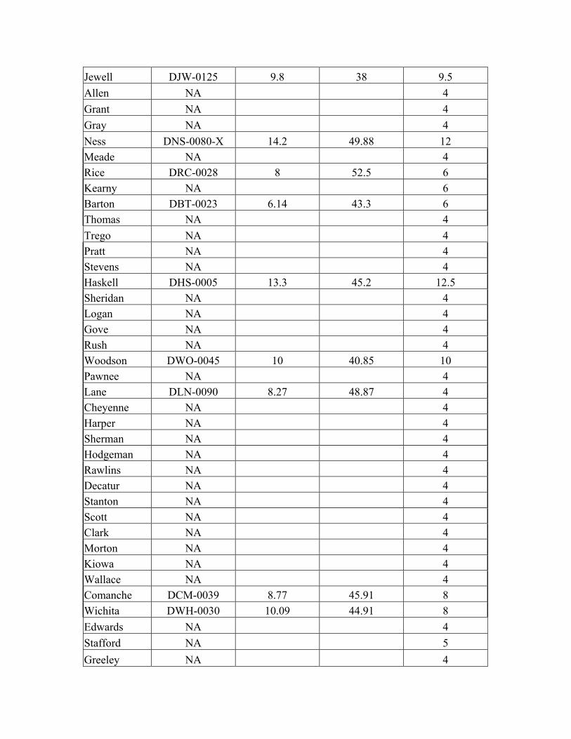
Jewell DJW-0125 9.8 38 9.5 Allen NA 4 Grant NA 4 Gray NA 4 Ness DNS-0080-X 14.2 49.88 12 Meade NA 4 Rice DRC-0028 8 52.5 6 Kearny NA 6 Barton DBT-0023 6.14 43.3 6 Thomas NA 4 Trego NA 4 Pratt NA 4 Stevens NA 4 Haskell DHS-0005 13.3 45.2 12.5 Sheridan NA 4 Logan NA 4 Gove NA 4 Rush NA 4 Woodson DWO-0045 10 40.85 10 Pawnee NA 4 Lane DLN-0090 8.27 48.87 4 Cheyenne NA 4 Harper NA 4 Sherman NA 4 Hodgeman NA 4 Rawlins NA 4 Decatur NA 4 Stanton NA 4 Scott NA 4 Clark NA 4 Morton NA 4 Kiowa NA 4 Wallace NA 4 Comanche DCM-0039 8.77 45.91 8 Wichita DWH-0030 10.09 44.91 8 Edwards NA 4 Stafford NA 5 Greeley NA 4

Table 1. The smallest water body still containing 50 acre/feet of water was used as a threshold for determining the size of water body that could be eliminated during post-processing of the water mask on a county by county or by physiographic region basis.

Figure 1. As we moved further west for this project, we had less data available per county to determine a threshold unique to each county for the elimination process and to identify a relationship between volume and area for the regression analysis. To solve this problem we consolidated data from counties that fit into the same physiographic region to keep as consistent as possible similar terrain and drainage patterns that partially determine volume.

The legal descriptions of recorded dam permits provided by the DWR were converted to both UTM coordinates (to match the projection of our imagery) and latitude and longitude as requested by the DWR. The points were imported into ARC and then converted to a shapefile in ArcView. The dam permits were superimposed over the water mask and recorded permits were evaluated. In order to view the database of permitted dams provided by the DWR, with the addition of geographic information, the individual county shape files can be joined to the table “dams_dwr”. The field used to join the two tables is the “Unique ID” field from the DWR table and the “county_pts15” (the second id field) field from the individual county shape files. Some tables have already been joined.

A point coverage was created by visual inspection of water bodies without dam permits. Both Landsat ETM+ imagery and 1 meter resolution aerial photography from Terra Server (http://terraserver.homeadvisor.msn.com/) were used to visually inspect and evaluate classified water bodies to determine whether further inspection was needed. Water bodies not flagged for further evaluation, but visible on the water mask, include

natural lakes (such as oxbow lakes), cooling ponds, and sewage treatment ponds. Some counties were particularly problematic because of their landscape. Barber County, in the Red Hills region of south-central Kansas, incorporated the largest number of unpermitted dams (58) as determined by our methods. The Red Hills region is full of caves, buttes, mesas, and sinkholes and are unique to this part of Kansas. Some of these water bodies we have labeled as dams could be natural water bodies but appear similar to dams in the satellite imagery. Toronto Lake in Woodson County did not have a permit from the DWR present, but we did not flag it as an unpermitted dam. There is also a dam in Geary County that does not have a legal coordinate with it, although the geographic coordinates are available. This is most likely because it is on Fort Riley, which does not fall under the township/range coordinates in the LEO program. The total number of water bodies identified for further inspection from the 70 counties completed this quarter is 413 (Table 2).

County # of Dams Marshall 14 Labette 4 Ford 3 Chase 8 Harvey 5 Reno 15 Chautauqua 3 Osborne 27 Wabaunsee 8 Russell 5 Wilson 28 Ellsworth 1 Anderson 35 Graham 2 Montgomery 16 Morris 6 Geary 1 Marion 2 Smith 3 Seward 1 Riley 0 Phillips 6 Rooks 7 Republic 1 Elk 13 Kingman 26

Hamilton 0 Cherokee 11 Mitchell 0 Barber 58 Washington 2 Sumner 10 Jewell 0 Allen 8 Grant 0 Gray 0 Ness 2 Meade 5 Rice 3 Kearny 0 Barton 1 Thomas 0 Trego 7 Pratt 6 Stevens 0 Haskell 0 Sheridan 1 Logan 1 Gove 3 Rush 4 Woodson 2 Pawnee 3 Lane 4 Cheyenne 0 Harper 9 Sherman 0 Hodgeman 1 Rawlins 1 Decatur 1 Stanton 1 Scott 0 Clark 14 Morton 0 Kiowa 11 Wallace 0

Comanche 0 Wichita 0 Edwards 1 Stafford 3 Greely 0 Table 2. Number of unpermitted dams by county.

The database for the unpermitted dams includes the legal description, county location, geographic coordinates, area and estimated volume. The area was calculated by converting each polygon (water body in square meters) to acres. Volume was estimated using linear regression analysis in SPSS software. The regression analysis was not used to eliminate water bodies smaller than 50 acre/feet; the minimum threshold value was used. A regression equation was determined by physiographic regions; error estimates and coefficients were also recorded. A regression analysis was not performed for the following counties― Riley, Hamilton, Mitchell, Grant, Gray, Kearny, Thomas, Jewell, Stevens, Haskell, Cheyenne, Sherman, Morton, Wallace, Comanche, Wichita, Greely, Riley- because no unpermitted dams were recorded. The High Plains regression analysis was based on the following counties― Cheyenne, Decatur, Thomas, Graham, Logan, Gove, Wichita, Lane, Stanton, Grant, Haskell, Stevens, Seward, and Meade counties. Other counties in the High Plains regions were not included because there was no data available. The Smokey Hills regression analysis was based on the following counties― Smith, Jewell, Republic, Washington, Rooks, Osborne, Mitchell, and Ellsworth counties.

Table 3. High Plains regression equation.

Table 4. Smokey Hills regression equation.

2. ArcView Database Contents The following information is provided with each county on the ArcView CD:

q) County water mask, r) County Landsat Thematic Mapper scene,

County High Plains Adj. R2 .959 F 674.57 B0 -71.272 B1 11.496 Equation V=-71.272+(11.496*Area)

County Smokey Hills Adj. R2 .928 F 429.023 B0 -15.097 B1 8.187 Equation V=-15.097+(8.187*Area)

s) Points where permitted dams exist according to the database provided by the DWR,

t) Points corresponding to water bodies that are most likely dams, but do not have permits,

u) A database for existing permitted dams containing dam ID’s, legal descriptions, area and volume information (if available), geographic coordinates and UTM coordinates,

v) A database for unpermitted dams containing legal descriptions, geographic coordinates, area and estimated volume,

w) Regression equation used to determine volume, x) The spatial threshold used to eliminate water bodies containing less than

50 acre/feet of water

3. Production Schedule The entire state has been completed.

the kansas dam inventory project114 - kars...

Documents