The light stop window

Antonio Delgadoa, Gian F. Giudiceb, Gino Isidorib,c,

Maurizio Pierinib, Alessandro Strumiad,e

(a) Department of Physics, University of Notre Dame, Notre Dame IN 46556, USA

(b) CERN, Theory Division, CH–1211 Geneva 23, Switzerland

(c) INFN, Laboratori Nazionali di Frascati, I-00044 Frascati, Italy

(d) Dipartimento di Fisica, Universita di Pisa and INFN Sez. Pisa, Pisa, Italy

(e) National Institute of Chemical Physics and Biophysics, Tallinn, Estonia

Abstract

We show that a right-handed stop in the 200–400 GeV mass range,together with a nearly degenerate neutralino and, possibly, a gluinobelow 1.5 TeV, follows from reasonable assumptions, is consistentwith present data, and offers interesting discovery prospects at theLHC. Triggering on an extra jet produced in association with stopsallows the experimental search for stops even when their mass dif-ference with neutralinos is very small and the decay products aretoo soft for direct observation. Using a razor analysis, we are able toset stop bounds that are stronger than those published by ATLASand CMS.

arX

iv:1

212.

6847

v2 [

hep-

ph]

20

Sep

2014

1 Introduction

Supersymmetry has been significantly cornered by LHC searches. The discovery of the

Higgs boson at 126 GeV [1,2] and the direct limits on sparticles rule out most of the natural

implementations of low-energy supersymmetry, at least in their simplest versions [3]. Pockets

of parameter space still survive, but their exploration requires the 14-TeV phase of the LHC.

At this stage, it is appropriate to examine the available experimental data and look for hints

that can guide us towards special regions where supersymmetry may still hide.

In this paper, we point out that there is a window of supersymmetric parameters that

(i) are well consistent with all collider data and flavor constraints, (ii) naturally emerge

from RG evolution of simple UV completions, (iii) predict the correct thermal abundance

for dark matter (DM), and (iv) give observable signals at LHC14. In this special window,

the supersymmetric mass spectrum has the following properties:

• The lightest stop is mostly right-handed and its mass is in the range mt1 = 200–

400 GeV.

• The heavy, mostly left-handed, stop has a much larger mass (in the 1–2 TeV range),

but it is correlated with the light stop in such a way that their geometric average is

mS ≡ (mt2mt1)1/2 ≈ 500–600 GeV.

• The stop trilinear term is large, such that1 A2t ≈ 6m2

S.

• The gluino mass is below about 1.5 TeV.

• The lightest neutralino has a mass slightly smaller than the lightest stop, by an amount

of about 30–40 GeV.

In section 2 we will give several arguments that lead to the mass spectrum described

above. None of them is sufficiently compelling to select conclusively the sparticle masses

but these arguments, taken together, give circumstantial evidence in favor of our choice of

parameters. Our conclusion is based on the following considerations:

• We choose the values of the stop parameters that minimize the average stop mass, while

leading to a Higgs mass of about 126 GeV. The resulting stop mass spectrum, although

not strictly natural, has the advantage of reducing the amount of unnaturalness forced

upon supersymmetry by present LHC data.

1This configuration is known as the “maximal mixing” case, although it does not necessarily imply alarge mixing between the two stop mass eigenstates, as discussed in sect. 2.

1

• Stops affect the rates for gg → h and h → γγ. Experimental data are at present

not sufficiently constraining, but will soon play an important role in selecting stop

parameters. In particular, we find that stop contributions to gg → h and h → γγ

exactly cancel for mt2 ≈ 6mt1 , under the conditions preferred by the Higgs mass value.

• Flavor constraints rule out a light left-handed stop, but are consistent with a light

right-handed stop. We also show that, if the CKM matrix is the only source of flavor

violation and the higgsino is relatively light, supersymmetric contributions can improve

the agreement with the measurements of εK , while being compatible with B → Xsγ.

This is achieved for a large mass splitting between left-handed and right-handed stops.

• A large splitting between left-handed and right-handed stop masses naturally emerge

from RG evolution, as long as the gluino is not too heavy. Moreover, once we require

a large stop mixing parameter at low energy, we find an upper bound on the gluino

mass.

• A light stop can be very helpful to obtain the right dark-matter relic density, which

is typically too large for B-ino LSP or too small for higgsino or W-ino LSP in generic

supersymmetric models. The process of coannihilation selects the preferred value of

the mass difference between stop and neutralino.

After we have determined the favorable region for sparticle masses, we study in sect. 3

the experimental strategies for discovery at the LHC. The phenomenology of supersymmet-

ric frameworks with light stop has been discussed at length in the recent literature (see

e.g. ref. [4–9]). The search of light stops has also been the focus of recent dedicated experi-

mental analyses by both ATLAS and CMS [10]. However, the peculiarity of our scenario is

the near mass-degeneracy between stop and neutralino, which makes experimental identifi-

cation especially arduous (see ref. [11–14] for previous attempts to address this problem).

On the one hand, we show that the decay t → Nb`ν`, which has been neglected in

the present exclusive experimental searches, can dominate over the more traditional decay

t → cN , especially if the mass difference between t and N is not too small. The four-body

decay process has the advantage of producing observable leptons in the final state, leading

to a possibly higher signal/background ratio in exclusive searches. On the other hand, by

an explicit simulation of this decay channel and the analysis of presently available data, we

show that the inclusive searches, and particularly the CMS razor analysis, already provides

significant constraints on this framework.

2

122

124

126

128

130130

-4 -2 0 2 4

1000

10000

300

3000

Stop mixing parameter

Ave

rage

stop

mas

sin

GeV

-0.05

0

0.05

0.1

0 100 200 300 400 500 6000

500

1000

1500

2000

2500

3000

Lightest stop mass mt�1

in GeV

Hea

vies

tsto

pm

ass

mt� 2

inG

eV

mt�1

> mt�2

m t� 2=

6mt� 1

mh < 125 GeV

Figure 1: The Higgs mass in low-energy super-symmetry for large tanβ ≈ 20. The shaded re-gion in the (Xt,mS) plane corresponds to theobserved value of mh. Higher-order correctionsand the uncertainty in the top mass amount toan error of a few GeV in mh.

Figure 2: The white region is the range in the(mt1

,mt2) plane allowed by the mh constraint,

while shaded regions are excluded. The full,dashed, and dotted lines correspond to fixed val-ues of ∆t, satisfying the mh constraint with|Xt| >

√6 (blue) or |Xt| <

√6 (black).

2 The light-stop window

2.1 Constraints from the Higgs mass and decay rates

The leading part of the supersymmetric prediction for the mass of the lightest Higgs boson

is

m2h = m2

Z cos2 2β +3y2

tm2t

4π2

[log

(m2S

m2t

)+X2

t

(1− X2

t

12

)]+ · · · (1)

where Xt = (At + µ cot β)/mS, m2S = mt1mt2 is the average stop mass, yt = mt/v is the

top-quark Yukawa coupling, and v ≈ 174 GeV is the Higgs vev. In fig. 1 we show the region

of the (Xt,mS) plane compatible with the observed Higgs mass (for tan β � 1), including

also the leading two-loop corrections to the Higgs mass not shown in eq. (1). The lightest

average stop mass that can lead to the observed Higgs mass is obtained for

mS ≈ 500 GeV and X2t ≈ 6 . (2)

We focus on such configuration, the so-called “maximal mixing” case, since it reduces the

fine-tuning in electroweak symmetry breaking and can lead to observable signals.

3

Further constraints on Xt and the stop masses can be obtained by examining the correc-

tions to the h→ γγ and h↔ gg rates:

Γ(h↔ gg)

Γ(h↔ gg)SM

= (1 + ∆t)2 ,

Γ(h→ γγ)

Γ(h→ γγ)SM

= (1− 0.28∆t)2 , (3)

where, in the limit in which we decouple the pseudoscalar Higgs, we find

∆t ≈m2t

4

(1

m2t1

+1

m2t2

− X2t

m2S

). (4)

Present data (fitted in the context of the SM plus light stops) give [15]

∆t = −0.04± 0.11 (5)

and do not yet imply a significant constraint, as it is clear from fig. 2 where we plot iso-curves

of ∆t after imposing the mh requirement. The situation will improve in the future. Note

that no deviations from the SM (∆t ≈ 0) are obtained for mt2 ≈ 6mt1 if we insist on having

X2t ≈ 6.

A few comments are in order:

• An independent indication of a large splitting between mt2 and mt1 can be obtained if

we assume that At is not significantly larger than the trace of the stop mass matrix.

Assuming A2t < a(m2

t1+m2

t2), then (for large tan β) X2

t is bounded by

X2t < a

m2t1

+m2t2

mt1mt2

r�1' a

r, r =

mt1

mt2

. (6)

Vacuum stability arguments imply a < 3 (assuming m2Hu� m2

t2), but this does not

allow us to deduce a significant constraint on r. However, if a ∼< 1 (as naturally

expected from RG arguments, see next section) then we are forced to assume small

values of r in order to reach X2t ≈ 6.

• Despite the large value of Xt, the mixing of the two stop eigenstates is suppressed in

the limit r � 1:

θt =1

2arcsin

(2mtmSXt

m2t2−m2

t1

)r�1' rXtmt

mS

. (7)

So, in this limit, we can approximately identify the two mass eigenstates with the

electroweak eigenstates. As we will show in the next section, it is natural to identify

the lightest state with an almost right-handed stop. Note also that for r � 1 the

lightest stop mass is significantly lighter than the average stop mass in eq. (2): r ≈ 1/6

corresponds to mt1 ≈ 200 GeV.

4

0 200 400 600 800 10000

1000

2000

3000

4000

1

2

3

4

5

6

7

8

9

10

Lightest stop mass in GeV

Glu

ino

mas

sin

GeV

Sto

pm

ass

rati

om

t�

2�m

t

1

Figure 3: Illustrative example of renormaliza-tion group evolution from the unification scaleto the weak scale of gaugino masses M1, M2,M3 (green curves), of the stop mass parametersmtL

and mtR(full and dashed blue curves, re-

spectively), ytAt (red dashed curve), mHu (blackcurve), in a configuration leading to mtR

� mtLat the weak scale. All masses are in GeV unitsand we assumed the MSSM.

Figure 4: Gluino and light-stop masses result-ing from a scan of the parameter space assum-ing universal scalar and gaugino masses, andthe condition |At| < 3m0, at the GUT scale.All points satisfy the mh ≈ 126 GeV con-straint and are colored according to the value ofmt2

/mt1, as indicated on the right-handed axis.

For illustrative purposes lines corresponding toM3/mt1

= 1, 2, 3, 4 are also shown.

2.2 Constraints from the RG evolution

A numerically large splitting between mtLand mtR

naturally arises from the evolution under

renormalization-group equations (RGE), provided scalar masses are significantly larger than

gaugino masses at the high scale [17]. This can be understood by looking at the one-loop

RGE for third generation squark masses and mHu . Neglecting off-diagonal flavor-mixing

terms we have

8π2dm2

tL

d log µ= y2

t Yt −16

3g2

3M23 − 3g2M

22 −

1

15g2

1M21 , (8)

8π2dm2

tR

d log µ= 2 y2

t Yt −16

3g2

3M23 −

16

15g2

1M21 , (9)

8π2 dm2Hu

d log µ= 3 y2

t Yt − 3g2M22 −

3

5g2

1M21 , (10)

where µ is the renormalization scale, and

Yt = m2tL

+m2tR

+m2Hu

+ A2t . (11)

5

The RG evolution of the stop masses depends mainly on two effects: the QCD term (g23M

23 )

and the Yukawa term (y2t Yt). If we take M3, mtL

and At to be comparable and in the range

1–2 TeV at the weak scale (in order to fulfill the mh constraints and the experimental bounds

on the gluino mass), we find that: i) QCD and Yukawa terms compensate to a large extent

in the running of mtL; ii) the Yukawa term is dominant during most of the running of mtR

,

leading to mtR� mtL

at the weak scale starting from the initial condition mtR= mtL

at

some high scale; iii) the Yukawa term is always dominant in the running of m2Hu

, which

naturally becomes negative at the weak scale.

An illustrative spectrum is shown in fig. 3a, where we required m2Hu

= −m2Z/2, M3 =

1.3 TeV, and mtR< 300 GeV at the weak scale, and adjusted At in order to achieve the

condition mtR= mtL

at 2× 1016 GeV. The corresponding weak-scale configuration is consis-

tent with all the existing experimental bounds, with the condition mh = 126 GeV (assuming

tan β ∼> 5), and with a light stop below 300 GeV. A few percent tuning in the initial values

of m2Hu

and the higgsino mass µ is necessary in order to achieve the correct pattern of elec-

troweak symmetry breaking, but this is unavoidable in the minimal supersymmetric model

with mh = 126 GeV. The soft-breaking terms needed to reach this low-energy configuration

require an initial splitting m2squarks/m

2gauginos ∼ 10 at the high-energy scale. All three genera-

tions of squarks can be degenerate at the high scale, since the separation of the right-handed

stop is fully driven by the dynamics of the low-energy degrees of freedom. In this case the

squarks of the first two generations would have a mild RGE evolution (reaching low-energy

values slightly above 2 TeV for the illustrative configuration shown in fig. 3a).

The dynamical separation between mtRand mtL

, together with the generation of a large

Xt, from high-scale RG running naturally occurs only in a limited range of gluino masses.

This can be understood by inspecting the expressions of At, mtRand mtL

at the weak scale

in models with a universal scalar mass m0 and trilinear coupling A0 at the GUT scale,

At ≈ 0.3A0 + 0.8M3 , (12)

m2tR≈ 0.5M2

3 − 0.07A20 − 0.10A0M3 + 0.3m2

0 , (13)

m2tL≈ 0.7M2

3 − 0.03A20 − 0.05A0M3 + 0.7m2

0 , (14)

where M3 is the gluino mass at the weak scale. From these equations it is clear that if

M3 � m0, |A0| a large splitting among the two stop masses and a large Xt are obtained only

for unnaturally large values of |A0|/m0. Similarly, maximal mixing and large splitting cannot

be obtained if M3 � m0, |A0|. The upper bound on M3, which is particularly important

for the LHC searches, is quantified in fig. 4, where we show the points satisfying the mh

constraint in the mt1–M3 plane. As can be seen, the gluino must satisfy the approximate

6

upper bound M3 ∼< 4mt1 , that implies M3 ∼< 1.6 TeV for the range of mt1 (mt1 ∼< 400 GeV)

corresponding to a large mt2/mt1 ratio.

As anticipated, in this framework m2Hu

naturally becomes negative at the weak scale

and the µ term must be properly adjusted to reproduce the correct value of mZ . Assuming

universal scalar masses at the high scale, m2Hu

runs very negative at the week scale, implying

|µ| > mtR, or heavy higgsinos. Alternatively, we can consider a scenario as in fig. 3, with

non-universal boundary conditions, where |µ| < mtRand thus higgsinos are lighter than the

right-handed stop. The two cases lead to a rather different phenomenology for flavor, dark

matter, and LHC searches.

2.3 Constraints from flavor physics

If some of the gauginos or higgsinos are not too heavy, a light stop can have a significant

impact on low-energy flavor-physics observables. On general grounds, even if gauginos and

higgsinos are in the several-TeV domain, sizable misalignments in flavor space between quark

and squark mass matrices are excluded. Therefore we assume that the light stop is mostly

right-handed and aligned in flavor space with the top quark. The remaining flavor violation

is described by the usual CKM angles in charged currents. An interesting and largely model-

independent correlation (controlled only by the size of |µ| and the stop mass parameters)

emerges between BR(B → Xsγ) and εK .

In the limit in which we retain only the effect of higgsinos and flavor-aligned right-handed

stop, the deviations from the SM in these two observables are described by

BR(B → Xsγ)

BR(B → Xsγ)SM

= 1− 2.5 ∆C7 − 0.7 ∆C8 , (15)

εKεSMK

= 1 + 1.9m2t

m2tR

F2

µ2

m2tR

, (16)

where

∆C7,8 = sin θt tan βµmt

m2tR

FLR7,8

µ2

m2tR

+m2t

m2tR

FRR7,8

µ2

m2tR

, (17)

and the normalization of the various loop functions (see Ref. [16,18] for the explicit expres-

sions) is

F LR7 (1) = −2

9, F LR

8 (1) = − 1

12, FRR

7 (1) =5

144, FRR

8 (1) =1

48, F2(1) =

1

12. (18)

For B → Xsγ we have expanded the result to first order in the stop-mixing angle. Note

that, even for | sin θt| � 1, the first term in eq. (17) can be sizable and can dominate over

7

Figure 5: Correlation between BR(B → Xsγ) and εK . The two ellipses denote the 68% and 90% CLexperimental range. All points reproduce the observed Higgs mass. The two black curves are obtainedvarying mtR

between 200 GeV and 400 GeV (from left to right) for mS = 500 GeV, µ = 250 GeV,and tanβ = 20 (dashed curve) or tanβ = 10 (full curve). The points are obtained varying theparameters in the range µ = [150− 400] GeV and mtR

= [200− 400] GeV, with mS < 700 GeV andtanβ = 20 (red) or tanβ = 10 (blue).

the second one, both because of the large value of the loop function F LR7 and because the mh

constraint favors tan β � 1. As a result, the experimental constraint on BR(B → Xsγ) puts

a very stringent bound on the maximal value of |θt| for higgsino masses of O(mtR), providing

a further argument in favor of a sizable hierarchy between the two stop mass eigenstates [see

eq. (7)]. The sign of the correction can be positive or negative, depending on the relative

sign of µ and At. The experimental data favor a constructing interference with the SM

amplitude: BR(B → Xsγ)exp/BR(B → Xsγ)SM = 1.09± 0.11.2

In the case of εK , the correction is always positive and, in first approximation, is inde-

pendent from the mixing angle. As a result, the present experimental constraint εexpK /εSM

K =

1.14± 0.10 [22] can be better satisfied if µ is not too heavy.

The correlation between the two observables is shown in fig. 5, where we restrict the

attention to the value of sgn(µAt) favored by BR(B → Xsγ). As can be seen, after imposing

the mh constraint and requiring |µ| ∼< 400 GeV, present data favor the configuration with

2This ratio is evaluated using the SM estimate from Ref. [19], and a naive average of the HFAG resultand the latest Babar result [21] on BR(B → Xsγ)exp.

8

Excl

uded

by

LH

C8

0.0 0.5 1.0 1.5 2.0

0

5

10

15

20

25

30

DM mass in TeV

DM

mas

ssp

litt

ing

inG

eV

Scalar color triplet Hstop�binoL

Therm

alabundance

Som

merfeld

included

Som

merfeld

neg

lected

Figure 6: Points in the supersymmetric parameter space that lead to the correct DM abundance.

mtR� mtL

that maximizes the correction to εK and minimizes the impact in BR(B → Xsγ).

2.4 Constraints from dark matter

A light stop offers the opportunity of curing the excessive relic abundance of B-ino LSP,

generally encountered in supersymmetric models. Indeed, the DM cosmological abundance

can be reproduced with a B-ino thermal relic that co-annihilates with stops if

mt1 = MDM + ∆M with ∆M ≈ 30 GeV. (19)

The relatively small mass difference arises imposing that the average annihilation cross sec-

tion equals

σvcosmo ≡ (2.3± 0.1)× 10−26 cm3s−1 (20)

at the freeze-out temperature Tf ≈ MDM/25. The dominant annihilation process is s-wave

stop annihilation into gluons (annihilation into quarks is p-wave suppressed):

σ(t1t∗1 → gg)v =

7 g43

432πm2t1

. (21)

Averaging over the components of the DM system (t and t∗ have 3 colors each, and the

neutralino has 2 polarisations) we get

σvcosmo = σ(t1t∗1 → gg)v ×

[1 +

e∆M/T

3(1 + ∆M/M)3/2

]−1

. (22)

9

The region where the DM abundance reproduces the cosmological values within 3 standard

deviations is shown as a red band in fig. 6 (see also [25]). In the figure we also show, as green

band, the result of a more precise computations that taks into account strong Sommerfeld

corrections [24].

3 Experimental signals

3.1 Stop decay rates

Beside gluino production, the most characteristic signal comes from the (mostly right-

handed) light stop. Dark matter considerations motivate the searches for a stop that is near

degenerate with the neutralino LSP, with a mass difference ∆M ≡ mt1 −MDM ≈ 30 GeV.

In this configuration, the stop is usually assumed to decay according to t1 → cN . Here we

point out that four-body stop decays (not suppressed by flavor-changing neutral currents)

can easily become competitive with the two-body flavor-violating decay. In the limit of small

∆M , the relevant stop decay widths are

Γ(t1 → cN) =2g2 tan2 θW θ2

tc ∆M2

9πmt1

= 100 cm−1

(θtc

10−5

)2 (∆M

30 GeV

)2(

400 GeV

mt1

), (23)

Γ(t1 → Nb`+ν`) =3 g6 tan2 θW ∆M8

70(6π)5M4W m2

t mt1

= 28 cm−1(

∆M

30 GeV

)8(

400 GeV

mt1

), (24)

as well as

Γ(t1 → Nbud) ≈ Γ(t1 → Nbcs) ≈ 3Γ(t1 → Nb`+ν`) ` = e, µ, τ . (25)

For the decay t1 → cN , the parameter θtc is the effective stop–scharm mixing angle. In

general, θtc is a free unknown parameter, since it depends on the flavor structure of the soft

terms. Assuming that it vanishes at some high scale ΛUV, a non zero value is generated

by RGE effects due to the SM Yukawa couplings (even in absence of other sources of flavor

violation) [26]. In our scenario, where t1 ≈ tR, the leading effect comes from an induced

tR–cL mixing, which can be estimated as

θMFVtc ∼ yty

2bVcbV

∗tb

16π2

vA

m2log

ΛUV

m= 3× 10−5

(2 TeV

m

)(log ΛUV/m

30

)(tan β

10

)2

, (26)

where we have omitted O(1) loop functions depending on mass ratios of heavy squarks and

charginos, whose average mass is denoted by m.

10

The t1 → Nb`+ν` decay receives contributions suppressed by heavy sparticles or mediated

only by virtual SM particles. We here focus on the latter contribution, which is dominant

in our case. This leads to eq. (24), whose derivation is given in the appendix, together with

the matrix element relevant for implementation in Monte Carlo codes.

The two decay channels can dominate in different regions of the parameter space and

become roughly comparable for θtc ∼ 10−5 and stop–neutralino mass differences motivated by

DM considerations. However, the large model dependence of θtc prevents us from making any

firm conclusion. The four-body decay has a much steeper dependence on ∆M and becomes

less relevant for very small ∆M . The decay t1 → Nb`+ν`, not previously considered in the

literature, is interesting from the experimental point of view since it leads to an additional

soft lepton.

Since the t1 → cN decay only produces an unobservable soft jet and its signatures have

been previously studied, in the following we focus our attention mainly on the four-body

decay channels in eqs. (24)–(25), which we assume to be the dominant decay modes. As

we discuss below, the bounds we are able to derive at present from existing LHC searches

are largely independent from this assumption; however, the presence of a lepton in the final

state could possibly lead to stringent bounds with future optimized searches (see sect. 3.3).

Assuming the four-body modes to be dominant implies

BR(t1 → Nb`+ν`) ≈ 1/9 (27)

for each lepton flavor `. Moreover, the smallness of the total decay width implies that the

decay vertex displacement may be detectable.

3.2 Bounds from existing LHC searches

The challenge of detecting stop decays for compressed spectra is all in the capability of

reconstructing and identifying the soft decay products of the two stop decays. On the other

hand, this is not the only experimental handle we have.

The first problem is with triggering these events. The jets and leptons originating from

the stop decay are too soft to be used to retain the events during on-line selection, given the

(CPU and bandwidth) budget of the experiments. The only possibility is to detect these

processes through the associate jet production (tt∗ plus one or more jets), with a consequent

reduction of the effective cross section.

In the worst case scenario, all the decay products are lost and one is left with one or more

11

[GeV]RM500 1000 1500 2000 2500

Pro

babi

lity

(a.u

.)

0

0.01

0.02

0.03

0.04

0.05

0.06

0.07

0.08 = 700χ∼ = 100 GeV m

t~m

= 1300χ∼ = 160 GeV m

t~m

= 1900χ∼ = 220 GeV m

t~m

= 2500χ∼ = 280 GeV m

t~m

= 3100χ∼ = 340 GeV m

t~m

= 3700χ∼ = 400 GeV m

t~m

2R0 0.2 0.4 0.6 0.8 1 1.2 1.4

Pro

babi

lity

(a.u

.)

0

0.02

0.04

0.06

0.08

0.1

0.12

0.14

0.16 = 700χ∼

= 100 GeV mt~m

= 1300χ∼ = 160 GeV m

t~m

= 1900χ∼ = 220 GeV m

t~m

= 2500χ∼ = 280 GeV m

t~m

= 3100χ∼ = 340 GeV m

t~m

= 3700χ∼ = 400 GeV m

t~m

MuEle MuMu EleEle Mu Ele Had

Pro

babi

lity

(a.u

.)

0

0.1

0.2

0.3

0.4

0.5

0.6

0.7

0.8

0.9 = 700χ∼ = 100 GeV m

t~m

= 1300χ∼ = 160 GeV m

t~m

= 1900χ∼ = 220 GeV m

t~m

= 2500χ∼ = 280 GeV m

t~m

= 3100χ∼ = 340 GeV m

t~m

= 3700χ∼ = 400 GeV m

t~m

Figure 7: Distribution of MR (left), R2 (center), and box-by-box event fraction (right) for pair-produced stop events as a function of the stop mass, for t → `ν`bN decays and mt −MDM = 30GeV. Even if this case is the most favorable for the selection of leptonic final states, the hadronicbox is the most populated due to the small value of mt −MDM.

jets: bounds exist from monojet searches [27,28] (performed in the Dark Matter context) and

from searches with ≥ 2 jets [29,31] (performed in supersymmetric contexts); see also [30].

In the best case scenario one can also detect the leptons from the decay of the stop pair.

This is why it is interesting to consider a set of analyses that focus on ≥ 2 jets for events

with or without leptons. The CMS razor analysis [32,33] is a all-in-one answer to our needs,

with the additional advantage that the jet selection in the analysis is looser than the one

used in the hadronic SUSY searches: pjetT > 60 GeV for the first two jet; pjet

T > 40 for the

other jets. The looser jet selection increases the effective cross section we are sensitive to.

To estimate the sensitivity of the search to the soft leptons from the stop decays, we

implemented an emulation of the razor analysis, based on generator-level jets and leptons.

We generate pair-produced stop squarks in√s = 7 TeV pp collisions using PYTHIA8 [34].

The stop are forced to decay with a flat matrix element as t → `ν`bN . The transverse

momenta of all the visible particles are summed to compute the missing transverse energy

at generator level. Similarly, these particles are clustered into jets using the FASTJET [35,36]

implementation of the antikT [37] algorithm. As for CMS, we use R = 0.5 to define the

jet size. The razor variables and the six boxes (MuEle, MuMu, EleEle, Mu, Ele, and Had)

are defined following the instructions provided by the CMS collaboration [38]. To take into

account the limited efficiency in lepton detection, we applied the efficiency curves of the CMS

dilepton SUSY search [39], using a hit-or-miss analysis. This is a valid procedure, since the

lepton definition in the razor and dilepton SUSY searches are similar.

We scan the value of the stop mass between 100 GeV and 400 GeV, fixing the stop-to-

neutralino mass gap to 30 GeV. We show in fig. 7 the distribution of the razor variables for

different stop masses, as well as the breakdown in boxes. A few important features should

be noticed:

12

i) The MR variable approximates the momentum of the jets in the frame such that

|pj1| = |pj2|. In the case of squark pair-production, for which this variable was designed,

this corresponds to the squarks rest frame. This is why the MR distribution for this

case peaks at the M∆ = (m2t1−M2

DM)/mt1 . Instead, in the case we consider here the

jets come from the associated (non-resonant) production and the peak is at ∼ 150

GeV, regardless of the stop and neutralino masses (due to the selection on the jet pT

and not to the SUSY kinematic).

ii) The R variable is defined as MTR/MR where MT

R ≤M∆ is a transverse invariant mass,

such that the QCD background peaks at R ∼ 0, while the signal can produce events

with larger values of R, where the two jets have similar directions, opposite to the

direction of the neutralinos. In the case of compressed stop spectra the R2 distribution

has some dependence on the stop mass, due to the correlation between the stop mass

(setting the scale of the hard interaction), the spectrum of the associated jets, and the

missing energy in the event.

iii) The majority of the events selected by the analysis falls in the hadronic box.

All these features are explained by the fact that the analysis is only sensitive to the events

with two associated jets. These jets form the hemispheres and the razor variables are com-

puted for a non-resonant production. In the largest fraction of the events the decay products

of the stop are not seen and, effectively, the signal behaves like for the direct production of

Dark Matter [40], The stop plays the part of the Dark Matter, with the big advantage of the

production cross section much larger than for Dark Matter direct detection. At the same

time, the result is largely independent on the final state the stop decays to.

These considerations suggest that the Had box is the only relevant sample to consider in

our study. This is also the only box for which the information needed for phenomenology

studies (observed yield and expected background vs R2 and MR) are given (the number of

expected background events is shown in fig. 8). While we limit our study to the Had box,

we stress the fact that there is some sensitivity in the Mu box and Ele boxes, which could

have be exploited if we had the relevant information. The importance of the Had box over

the others also implies that the monojet analysis is a good candidate to look for our signal,

as it is for Dark Matter direct production. The

We show in fig. 9 the limits obtained with the monojet and the razor (Had-only) anal-

yses. For both the analyses, we consider the expected background yield (with error) and

the observed yield, and we model the likelihood according to a Poisson distribution. The

background uncertainty is described using a log-normal function. We assign a 30% error

13

hEXP_pxEntries 751

Mean 688.4

RMS 181.1

[GeV]RM500 1000 1500 2000 2500 3000 3500

Num

ber

of E

vent

s

1

10

210

310

hEXP_pxEntries 751

Mean 688.4

RMS 181.1

hEXPhEXP_py

Entries 751

Mean 0.3277

RMS 0.07368

2R0.2 0.25 0.3 0.35 0.4 0.45 0.5

Num

ber

of E

vent

s

0

100

200

300

400

500

600

700

800hEXP_py

Entries 751

Mean 0.3277

RMS 0.07368

hEXP

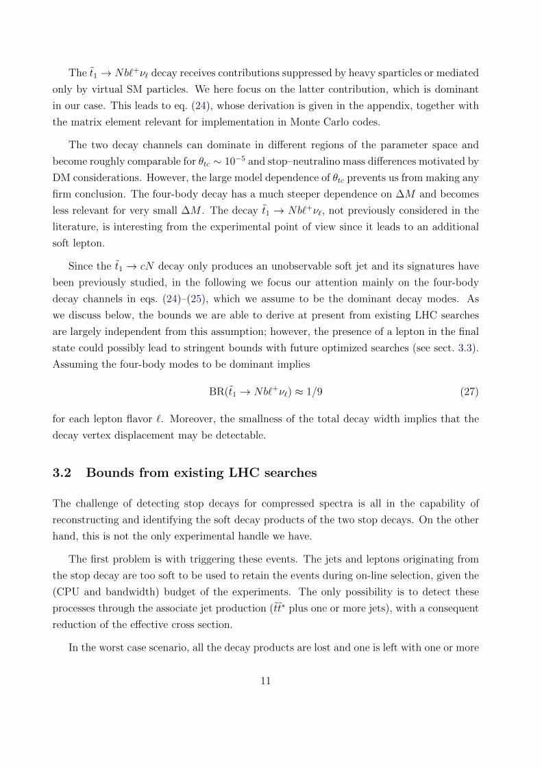
Figure 8: Projections of the expected background in the razor hadronic box, obtained from the bin-by-bin expected background in the

√s = 7 TeV run of CMS (from ref. [33, 38]).

to the signal efficiency, to take into account the differences between our implementation

of the analysis and a more realistic description of the CMS detector. We then derive a

posterior-probability density function for the signal cross section as:

P (σ) =∫ ∞

0db∫ 1

0dε

(b+ Lσε)ne−b−Lσε

n!Ln(ε|ε, δε) Ln(b|b, δb) (28)

where b (ε) is the actual value for the background yield (the efficiency), b (ε) is its expected

value, and δb (δε) the associated error; Ln(x|m, δ) is a log-normal function for x with mean

m and variance σ; n is the observed yield, L is the available luminosity (for which we neglect

the ∼ 4% error) and σ is the signal cross section. In the case of the razor analysis, the actual

posterior is obtained as the product of the posteriors in each of the bins provided in [38].

We verified that taking L = ε = 1 we can reproduce the limit on the signal strength for the

two analyses. The 95%-probability limit is obtained integrating the posterior from 0 up to

the value σUP such that ∫ σUP0 P (σ)dσ∫∞0 P (σ)dσ

= 0.95. (29)

The left plot of fig. 9 shows the 95%-probability limit on the signal cross section as a

function of the stop mass for both the analyses, fixing the mass split at 30 GeV and 100 GeV

(with the stop decayed to t∗N). The sensitivity of the monojet analysis is limited by the

tight selection on jets and missing transverse energy. The limit is worse for larger splitting

because of the veto on any third jet with pT > 30 GeV. At the contrary, the razor analysis

is more efficient for this signature and more performant for larger splitting, since no veto is

applied. One should also consider that at large values of the mass splitting the five leptonic

boxes could further improve the sensitivity.

14

[GeV]t~m

100 150 200 250 300 350 400

[pb]

σ

1

10

210

310

cross sectiont~ t

~NLO+NLL SUSY

M = 30 GeV∆CMS Razor Analysis

M = 90 GeV∆CMS Razor Analysis

M = 30 GeV∆CMS Monojet Analysis

M = 90 GeV∆CMS Monojet Analysis

CMS razor

hadronic only

our analysis

4.7 fb-1

7 TeV

HredL

ATLAS, 8 TeV Hdotted, yellowLCMS, 8 TeV Hdot-dashed, blueL

DM

line

t� 1®

Nb{

Ν

t� 1®

Nt

t� 1®

Nc

t� 1®

NbW

t�1 LSP

0 200 400 600 8000

100

200

300

400

500

Lightest stop mass in GeVN

eutr

alin

om

ass

inG

eV

Figure 9: Left: predicted cross section and experimental limits as functions of the lightest stopmass. Right: excluded regions in the (mt1

,MDM) plane from our re-analysis of 7 TeV data (red)compared with latest ATLAS (dotted regions shaded in yellow) and CMS (dot-dashed regions shadedin green) analyses of 8 TeV data.

The right plot of fig. 9 shows the limit in the stop mass vs neutralino mass plane. This

plot shows the same qualitative features as the 1D limit plot. At large splits, the limit from

the razor analysis is found to be consistent with (and slightly worse than) the official limit on

stop pair production [33]. Both the 1D and 2D limits were obtained comparing the excluded

cross section with the NLO+NLL tt∗ cross section at 7 TeV taking the decoupling limit for

the other SUSY particles [41].3

3.3 Dedicated analyses

The existing limit is interesting, considering how challenging this signature is. This study

also shows once more that the inclusive searches by ATLAS and CMS are much more general

than the signal signatures they have been designed for. While a dedicated search could do

better for a specific scenario, the inclusive searches are a good assurance policy for unexpected

signatures. Repeating the analysis at 8 TeV with more data will certainly push the sensitivity

further. On the other hand, we think it is interesting to imagine how the analyses could be

3In the revised version of the plot (september 2014) we subtract the signal contribution in the sideband tothe background estimate by CMS. This effect, generically negligible in the models considered by the originalanalysis, becomes relevant in our study for large values of the stop-neutralino mass splitting. Furthermore,we plot the latest bounds from ATLAS and CMS with 8 TeV data.

15

[GeV]T

muon p0 10 20 30 40 50 60 70 80 90 100

Pro

babi

lity

0

0.1

0.2

0.3

0.4

0.5

0.6

0.7W+jets

= 235 GeVLSP

= 250 GeV mt~ +jets mt~ t~

= 235 GeVLSP

= 300 GeV mt~ +jets mt~ t~

[GeV] t~m

100 150 200 250 300

[pb]

σ

1

10

M = 15 GeV∆CMS Monojet Analysis

M = 15 GeV∆Modified Monojet+MU Analysis

Figure 10: Improvements that can be obtained with a dedicated search. Left: distribution of themuon pT for W+jets and stop-pair events passing the CMS monojet selection criteria, except forthe muon veto and the veto on isolated tracks. Right: expected excluded cross section for stop pairproduction obtained from the CMS monojet analysis (blue) and a modified monojet+muon search(black). Events are generated with four-body stop decays to ff ′bN , of which ∼ 20% produce onemuon.

changed to improve the sensitivity.

One could certainly gain by using looser kinematic requirements. The limiting factor

is related to the triggers. For example, it was pointed out extending the razor analysis at

the tail of R2 for low MR could improve the sensitivity to DM production [40]. The same

conclusion applies to compressed stop-neutralino spectra, since the signature in the razor

Had box is the same.

A change in the lepton selection could further increase the sensitivity of these analyses.

The left plot on Fig. 10 shows the distribution of the muon pT for W+jets events selected

by the CMS monojet analysis, before applying the muon veto and the isolated track veto.

This is compared to the equivalent distribution obtained for events with pair-produced stops,

decaying to W ∗bN , with at least one of the two W ∗ producing a µν pair. We consider two

values of the stop mass (mt = 150 GeV and mt = 270 GeV) for ∆M = 15 GeV. Requiring

one muon with pT < 15 GeV corresponds to reducing the Z(νν)+jets background to a

negligible level, and to rejecting ∼ 92% of the other backgrounds.

To evaluate the potential improvement due to this change, we applied the monojet anal-

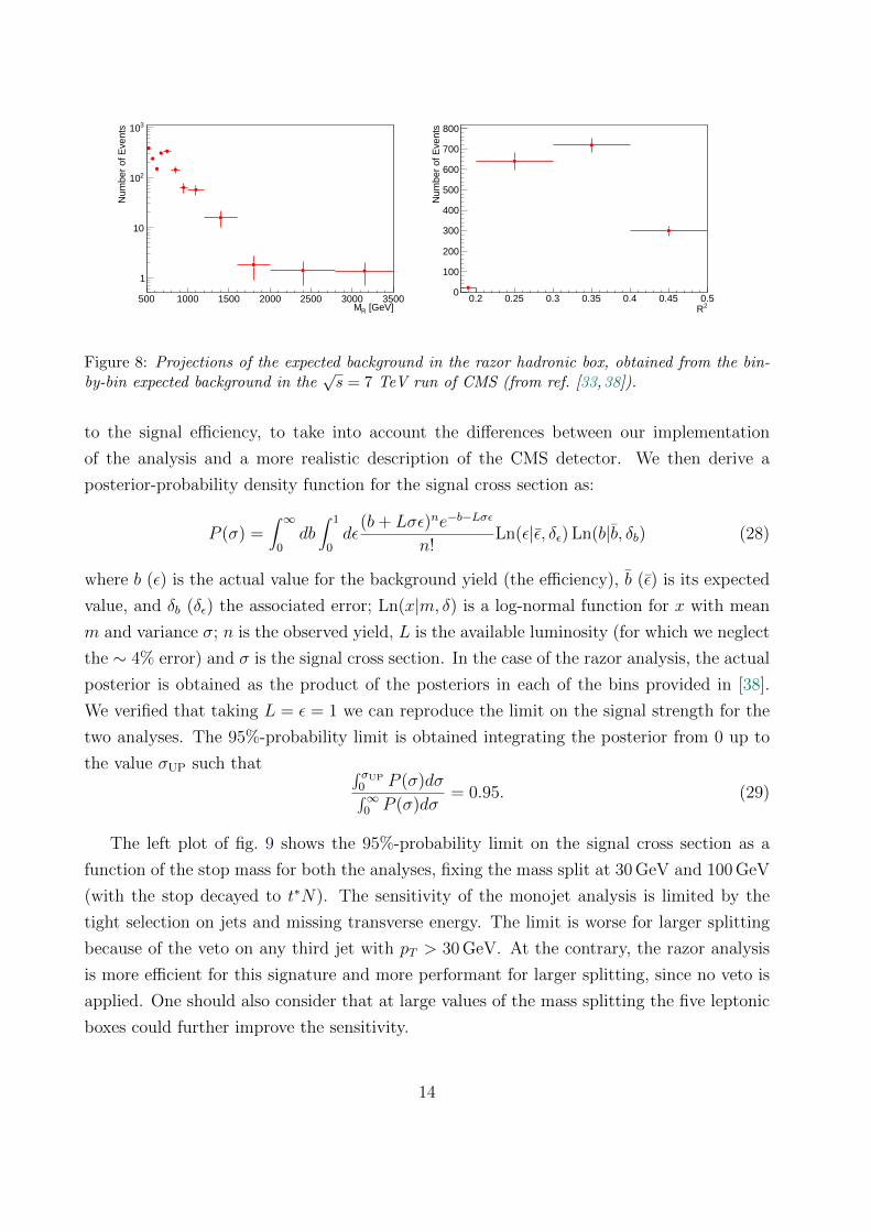
16

ysis to the generated stop-stop samples, and we separate the selected events in two boxes

(as for the razor analysis): the Muon box, including all the events with one muon with

pT < 15 GeV; the Had box, with all the other events. We then distribute the background

in the two boxes as follows: all the Z(νν)+jets background to the Had box; 8% (92%) of

the other background in the Mu (Had) box. We then evaluate the potential sensitivity of

this modified analysis on a sample of pair-produced stop decays, decaying to W ∗bN , 20% of

which produce at least one muon in stop decay.

The right plot of Fig. 10 shows the expected exclusion limit, compared to what is obtained

with the usual monojet analysis. A similar improvement could be used for electrons, provided

the understanding of the electron identification and the fake rate at low pT . One should keep

in mind that our results come from a simplified description of the CMS detector. A more

accurate assessment of the improvement can only be obtained with a detailed simulation

of the detector performances. We look forward to see this change applied to the monojet

analyses by ATLAS and CMS.

As a side remark, we would like to stress the fact that the stop decay products could

be displaced from the primary vertex of the proton-proton collision. Requiring a displaced

vertex, particularly with one muon originating from it, can potentially reduce the standard

model background to a very small level. However for ∆M ≈ 30 GeV only a small fraction

of the t1 decay after a detectable path of about 1 mm. An accurate estimate of the signal

sensitivity for a diplaced-vertex analysis would require an accurate description of the vertex

resolution for the LHC detectors and should be investigated directly by the ATLAS and CMS

collaborations. Even if the signal reduction is too large to be beneficial for 8 TeV searches,

this is an interesting possibility in light of the high statistics expected for the future 14 TeV

LHC run.

4 Conclusions

We have put forward a series of theoretical arguments that motivate the existence of a mainly

right-handed stop in the mass range mt1 = 200–400 GeV, together with a neutralino 30–

40 GeV lighter and, possibly, a gluino with mass below 1.5 TeV. However, quite independently

of any of these specific motivations, the search for stops nearly degenerate with the neutralino

LSP is an important experimental task, necessary to cover possible corners of parameter

space where supersymmetry may still hide.

We have pointed out that, when the mass splitting between stop and neutralino is smaller

17

than MW + mb, the previously-neglected four-body decay processes t1 → Nb`+ν` and t1 →Nbqq′ can compete with the flavor-changing decay t1 → cN . The presence of a charged

lepton in the final state of the four-body decay gives a useful handle to identify the stop in

this experimentally difficult mass configuration where all visible particles are relatively soft.

Regardless of the particular stop decay mode, the request of an extra jet in association

with the stop pair greatly improves triggering capability and signal identification. We have

shown that the inclusive searches using razor analysis are very efficient to probe stops nearly

degenerate with neutralinos. In this region of mass parameters, we are able to set limits on

the stop that are stronger than those published by ATLAS and CMS. Our limits (shown

in fig. 9) extend up to stop masses of about 250 GeV, even for a vanishing stop–neutralino

mass difference. This means that the LHC has already started to probe the “light stop

window” motivated by our theoretical considerations, but most of the interesting region will

be explored only at LHC14.

Note Added

While our paper was being completed, similar results were presented in [42, 43]. In our analysiswe used the response function for the CMS detector, provided by the CMS collaboration, insteadof trying to emulate the LHC detectors. More importantly, we used the full likelihood providedby the CMS collaboration for the inclusive razor analysis, which gives a realistic description of thelikelihood resulting from the data. This prevented us from extending our study to the razor btagsearch [44]. The latter has a better sensitivity in presence of bjets with pT > 40 GeV (i.e. farfrom the diagonal of the mχ0 vs. mt plane), if an accurate emulation of the btag efficiency and themistag rate is reached. On the diagonal, only a small fraction of the associated jets are bjets, suchthat requiring a btag has the effect of reducing the expected signal much more than the factor-threebackground reduction.

Acknowledgments

AD was partly supported by the National Science Foundation under grants PHY-0905383-ARRAand PHY-1215979. AS was supported by the ESF grant MTT8 and by SF0690030s09 project.

Appendix

In this appendix we derive the four-body stop decay width given in eq. (24). In the limit of smallmass difference (∆M �MW ,mt), the amplitude for pure right-handed stop decay tR → Nbe+ν is

|A |2 =32g6 tan2 θW

9M4Wm

2t

(PN · Pe)(Pb · Pν) , (30)

18

where Pi are the quadri-momenta of the particles involved. The decay width is given by

Γ =

∫dφ(4) |A |2

2mt

. (31)

The 4-body phase space integral dφ(4) can be analytically performed at leading order in ∆M =mt−MDM. Indeed, by writing the decay as t→ XY → (Ne)(bν), the amplitude for each sub-decayis separately Lorentz invariant. Thus, using

dφ(4) =dsXdsY(2π)2

dφ(2)(t→ XY )dφ(2)(X → Ne)dφ(2)(Y → bν) , (32)

|A |2 =8g6 tan2 θW

9M4Wm

2t

sX (sY −M2DM) , (33)

we get

Γ =

∫ m2t

M2DM

dsY

∫ (mt−√sY )2

0dsX

(1− M2

DM

sY

)λ(m2

t, sX , sY )|A |2

4(4π)5m3t

=2g6 tan2 θW I

9(4π)5M4Wm

2tmt

, (34)

I ≡ m8t

∫ 1

M2DM/m

2t

dy

∫ (1−√y)2

0dx

x

y

(y − M2

DM

m2t

)2√(1 + x− y)2 − 4x ≈ 8 ∆M8

315, (35)

where we have kept only the leading order in ∆M . From these expressions we obtain eq. (24).

References

[1] ATLAS Collaboration, Phys. Lett. B 716 (2012) 1 [arXiv:1207.7214].

[2] CMS Collaboration, Phys. Lett. B 716 (2012) 30 [arXiv:1207.7235].

[3] See e.g. A. Strumia, JHEP 1104 (2011) 073 [arXiv:1101.2195].

[4] R. Barbieri and D. Pappadopulo, JHEP 0910 (2009) 061 [arXiv:0906.4546].

[5] M. Papucci, J. T. Ruderman and A. Weiler, JHEP 1209 (2012) 035 [arXiv:1110.6926].

[6] C. Brust, A. Katz, S. Lawrence and R. Sundrum, JHEP 1203 (2012) 103 [arXiv:1110.6670].

[7] Z. Han, A. Katz, D. Krohn and M. Reece, JHEP 1208 (2012) 083 [arXiv:1205.5808].

[8] J. R. Espinosa, C. Grojean, V. Sanz and M. Trott, arXiv:1207.7355 [hep-ph].

[9] M. Carena, G. Nardini, M. Quiros and C. E. M. Wagner, JHEP 0810 (2008) 062 [arXiv:0806.4297].

[10] https://twiki.cern.ch/twiki/bin/view/AtlasPublichttp://cms.web.cern.ch/org/cms-papers-and-results

[11] C. -L. Chou and M. E. Peskin, Phys. Rev. D 61 (2000) 055004 [hep-ph/9909536].

[12] G. Hiller, J. S. Kim and H. Sedello, Phys. Rev. D 80 (2009) 115016 [arXiv:0910.2124 [hep-ph]].

[13] D. S. M. Alves, M. R. Buckley, P. J. Fox, J. D. Lykken and C. -T. Yu, arXiv:1205.5805.

[14] C. Kilic and B. Tweedie, arXiv:1211.6106.

19

[15] The result is obtained updating the fit of P. P. Giardino, K. Kannike, M. Raidal and A. Strumia,arXiv:1207.1347.

[16] M. Ciuchini, G. Degrassi, P. Gambino and G. F. Giudice, Nucl. Phys. B 534 (1998) 3 [hep-ph/9806308].

[17] A. Strumia, Phys. Lett. B 397 (1997) 204 [hep-ph/9609286].

[18] E. Gabrielli and G. F. Giudice, Nucl. Phys. B 433 (1995) 3 [Erratum-ibid. B 507 (1997) 549] [hep-lat/9407029].

[19] M. Misiak, H. M. Asatrian, K. Bieri, M. Czakon, A. Czarnecki, T. Ewerth, A. Ferroglia and P. Gambinoet al., Phys. Rev. Lett. 98 (2007) 022002 [hep-ph/0609232].

[20] Heavy Flavor Averaging Group Collaboration, arXiv:1207.1158.

[21] BABAR Collaboration, arXiv:1207.5772.

[22] A. J. Bevan et al., PoS HQL 2010 (2011) 019 [http://utfit.org/UTfit].

[23] C. Boehm, A. Djouadi and Y. Mambrini, Phys. Rev. D 61 (2000) 095006 [hep-ph/9907428].

[24] A. De Simone, G. F. Giudice and A. Strumia, JHEP 1406 (2014) 081 [arXiv:1402.6287].

[25] M. Farina, M. Kadastik, D. Pappadopulo, J. Pata, M. Raidal and A. Strumia, Nucl. Phys. B 853 (2011)607 [arXiv:1104.3572]. M. Kadastik, K. Kannike, A. Racioppi and M. Raidal, JHEP 1205 (2012) 061[arXiv:1112.3647].

[26] G. Hiller and Y. Nir, JHEP 0803 (2008) 046 [arXiv:0802.0916].

[27] CMS Collaboration, JHEP 1209, 094 (2012) [arXiv:1206.5663].

[28] ATLAS Collaboration, arXiv:1210.4491.

[29] ATLAS Collaboration, Phys. Lett. B 710, 67 (2012) [arXiv:1109.6572].

[30] ATLAS conference note 2012-166.

[31] CMS Collaboration, arXiv:1210.8115.

[32] C. Rogan, arXiv:1006.2727.

[33] CMS Collaboration, arXiv:1212.6961.

[34] T. Sjostrand, S. Mrenna and P. Z. Skands, Comput. Phys. Commun. 178, 852 (2008) [arXiv:0710.3820].

[35] M. Cacciari, G. P. Salam and G. Soyez, Eur. Phys. J. C 72, 1896 (2012) [arXiv:1111.6097].

[36] M. Cacciari and G. P. Salam, Phys. Lett. B 641, 57 (2006) [hep-ph/0512210].

[37] M. Cacciari, G. P. Salam and G. Soyez, JHEP 0804, 063 (2008) [arXiv:0802.1189].

[38] The details on how to implement the CMS razor analyses outside the CMS analysis framework aregiven in https://twiki.cern.ch/twiki/bin/view/CMSPublic/RazorLikelihoodHowTo.

[39] CMS Collaboration, JHEP 1208, 110 (2012) [arXiv:1205.3933].

[40] P. J. Fox, R. Harnik, R. Primulando and C. -T. Yu, Phys. Rev. D 86, 015010 (2012) [arXiv:1203.1662].

[41] M. Kramer, A. Kulesza, R. van der Leeuw, M. Mangano, S. Padhi, T. Plehn and X. Portell,arXiv:1206.2892.

20

[42] Z.-H. Yu, X.J. Bi, Q.-S. Yan, P.-F. Yin, arXiv:1211.2997.

[43] K. Kriza, A. Kumar, D.E. Morissey, arXiv:1212.4856.

[44] CMS Collaboration, CMS-PAS-SUS-11-024.

21