The LMDZ4 general circulation model: climate

performance and sensitivity to parametrized physics

with emphasis on tropical convection

Frederic Hourdin, Ionela Musat, Sandrine Bony, Pascale Braconnot, Francis

Codron, Jean-Louis Dufresne, Laurent Fairhead, Marie-Angele Filiberti,

Pierre Friedlingstein, Jean-Yves Grandpeix, et al.

To cite this version:

Frederic Hourdin, Ionela Musat, Sandrine Bony, Pascale Braconnot, Francis Codron, et al..The LMDZ4 general circulation model: climate performance and sensitivity to parametrizedphysics with emphasis on tropical convection. Climate Dynamics, Springer Verlag, 2006, 19,pp.3445-3482. <10.1007/s00382-006-0158-0>. <hal-00113202>

HAL Id: hal-00113202

https://hal.archives-ouvertes.fr/hal-00113202

Submitted on 13 Nov 2006

HAL is a multi-disciplinary open accessarchive for the deposit and dissemination of sci-entific research documents, whether they are pub-lished or not. The documents may come fromteaching and research institutions in France orabroad, or from public or private research centers.

L’archive ouverte pluridisciplinaire HAL, estdestinee au depot et a la diffusion de documentsscientifiques de niveau recherche, publies ou non,emanant des etablissements d’enseignement et derecherche francais ou etrangers, des laboratoirespublics ou prives.

The LMDZ4 general circulation model: climate

performance and sensitivity to parametrized physics with

emphasis on tropical convection

Frederic Hourdin∗1, Ionela Musat1, Sandrine Bony1, Pascale Braconnot2, Francis Codron1,

Jean-Louis Dufresne1, Laurent Fairhead1, Marie-Angele Filiberti3, Pierre Friedlingstein2,

Jean-Yves Grandpeix1, Gerhard Krinner4, Phu LeVan1, Zhao-Xin Li1, Francois Lott1

1 Laboratoire de Meteorologie Dynamique, LMD/IPSL, Paris2 Laboratoire des Sciences du Climat et de l’Environnement, LSCE/IPSL, Saclay

3 Institut Pierre Simon Laplace, IPSL, Paris4 Laboratoire de Glaciologie et Geophysique de l’Environnement, Grenoble.

Submitted to Climate Dynamics

Submitted, May 2005, Revised, December 22, 2005

Abstract

The LMDZ4 general circulation model is the atmo-spheric component of the IPSL-CM4 coupled modelwhich has been used to perform climate change simu-lations for the 4th IPCC assessment report. The mainaspects of the model climatology (forced by observedsea surface temperature) are documented here, as wellas the major improvements with respect to the previousversions, which mainly come form the parametrizationof tropical convection. A systematic methodology isproposed to help analyse the sensitivity of the tropi-cal Hadley-Walker circulation to the parametrizationof cumulus convection and clouds. The tropical cir-culation is characterized using scalar potentials asso-ciated with the horizontal wind and horizontal trans-port of geopotential (the Laplacian of which is pro-portional to the total vertical momentum in the atmo-spheric column). The effect of parametrized physics isanalysed in a regime sorted framework using the verti-cal velocity at 500 hPa as a proxy for large scale verti-cal motion. Compared to Tiedtke’s convection scheme,used in previous versions, the Emanuel’s scheme im-

∗Corresponding author address: Laboratoire de MeteorologieDynamique, UPMC, Tr 45-55, 3eme et., B99, F-75252 ParisCedex 05, FRANCE; E-mail : hourdin@lmd.jussieu.fr; Tel : 33-1-44278410; Fax: 33-1-44276272

proves the representation of the Hadley-Walker cir-culation, with a relatively stronger and deeper largescale vertical ascent over tropical continents, and sup-presses the marked patterns of concentrated rainfallover oceans. Thanks to the regime sorted analyses, thisdifferences are attributed to intrinsic differences in thevertical distribution of convective heating, and to thelack of self-inhibition by precipitating downdraughts inTiedtke’s parametrization. Both the convection andcloud schemes are shown to control the relative impor-tance of large scale convection over land and ocean,an important point for the behaviour of the coupledmodel.

1 Introduction

A great amount of effort has been spent in the past fewyears by climate modellers to prepare improved climatemodels suited to climate change simulations, in supportof the 4th assessment report of the IntergovernmentalPanel on Climate Change (IPCC).

Climate change modelling is a particular exercisein that the sensitivity of the model to anthropogenicforcing can hardly be assessed with respect toobservation. Because of uncertainties in radiativeforcing and because of climate internal variability,

1

the observed 20th century climate change does notyet provide a strong constraint on climate sensitivity(Wigley et al., 1997; Gregory et al., 2005). To overcomethis difficulty, one can use however the climatevariations observed in the past decades or paleoclimaterecords in order to identify key mechanisms involvedin the climate sensitivity, which may then serve asa guide for validation of the model and improvementof its physical content. A key issue in thatrespect is the representation of unresolved subgrid-scale processes accounted for in climate models throughparametrizations, in which the complexity of the realworld is reduced to a few deterministic equations. Afull climate change prediction, for a given “scenario”of anthropogenic emissions, also requires appropriatetreatment of ocean thermodynamics and circulation,water budget including routing from continentalsurfaces to the ocean, as well as computation of theevolution of the atmospheric composition, under theeffect of bio-geochemical processes for carbon dioxideor chemistry for methane or ozone.

The general circulation model LMDZ4 presentedhere is the atmospheric component of the IPSL-CM4version of the Institut Pierre Simon Laplace CoupledModel (Marti et al., 2005), developed with the abovementioned perspective in mind, and recently used toproduce climate change simulations for IPCC (Dufresneet al., 2005). With respect to the previous LMDZ3version (Li, 1999; Li and Conil, 2003), the major changein terms of physical content concerns the representationof cumulus convection, the Tiedtke (1989) schemebeing replaced by the Emanuel (1991, 1993) scheme.After the development and tuning of LMDZ4, anotherversion was derived which only differs by the use ofTiedtke’s scheme in place of Emanuel’s for convection.Both versions are presented here. They will be usedin a companion paper to analyse the role of theparametrized convection on the coupled climate andclimate sensitivity (Braconnot et al., in preparation).

Here we relate some characteristic behaviours ofthose very different parametrizations to the changesobserved in the simulated climate and large-scalecirculation. This question is generally difficult toaddress because the cumulus convection and large-scale circulation are tightly coupled. To overcomethis difficulty, we propose the following methodology:we characterize on the one hand the parametrizationbehaviour for a given large-scale regime using themonthly mean of the vertical velocity as a proxy forthe large-scale circulation, a framework proposed byBony et al. (1997) to analyse cloud radiative forcingand feedbacks; on the other hand, we characterizethe impact of those different parametrizations on the

large-scale circulation using the velocity potential aswell as a z-weighted potential, the Laplacian of whichcorresponds approximately to the vertical momentumof atmospheric columns. Note that the main focushere is not to discuss the impact of one particularaspect of the convective parametrization such asclosure, triggering or entrainment. A better strategyfor that would be to vary parts of one particularconvection scheme (see e. g., Jakob and Siebesma,2003; Grandpeix et al., 2005).

Major model improvements and tunings are firstpresented in section 2. Then we document in section3 some aspects of the simulated climate. Finally insection 4, we analyse in more details the sensitivityof the simulated climate to the parametrized physicswith a focus on the relationships between tropicalconvection and divergent circulation. One goal of thispaper is to serve as a reference for the analysis ofthe IPCC simulations, so that the model content andclimatology are described in some details. For readerswho would like to concentrate on the sensitivity analysisconcerning the tropical convection and Hadley-Walkercirculation and on methodological aspects, sections 2.3,2.4 and 3.2 may be sufficient to introduce the core ofthe discussion (sections 4.3 and 4.4).

2 Model description

2.1 LMDZ

LMDZ is the second generation of a climate modeldeveloped at Laboratoire de Meteorologie Dynamique(Sadourny and Laval, 1984; Le Treut et al., 1994; LeTreut et al., 1998). The dynamical equations arediscretised on the sphere in a staggered and longitude-latitude Arakawa C-grid (see e. g. Kasahara, 1977).The grid is stretchable (the Z of LMDZ standingfor Zoom capability) so that the model can be usedfor climate studies at both global (Li, 1999; Li andConil, 2003) and regional scale (Krinner and Genthon,1998; Genthon et al., 2002; Zhou and Li, 2002; Poutouet al., 2004; Krinner et al., 2004). The discretizationensures numerical conservation of both enstrophy(square of the wind rotational) for barotropic flows(following Sadourny, 1975b,a) and angular momentumfor the axi-symmetric component. The finite-differenceformulation thus correctly represents the enstrophytransfer from large to small scales of motions, down togrid-scale cut-off. An horizontal dissipation is addedto the dynamical equations. Based on an iteratedLaplacian, it is designed so as to represent properlythe pumping of enstrophy at the cut-off scale. Thetime step is bounded by a CFL criterion on the fastest

2

gravity modes. For the applications presented here,with a uniform resolution of 3.75◦ in longitude and2.5◦ in latitude, the time-step is 3 minutes. Forlatitudes poleward of 60 degrees in both hemispheres,a longitudinal filter is applied in order to limit theeffective resolution to the one at 60 degrees. The timeintegration is done using a leapfrog scheme, with aperiodic predictor/corrector time-step. On the vertical,the model uses a classical hybrid σ−p coordinate1. Thestandard version is based on 19 layers2 with the first4 layers in the first kilometre above surface, a meanvertical resolution of about 2 km between 2 and 20 kmand 4 layers above 20 km.

Both vapour and liquid water are advected witha monotonic second order finite volume scheme(Van Leer, 1977; Hourdin and Armengaud, 1999). Thisscheme is used also for the simulation of the directand inverse transport of trace species (Hourdin andIssartel, 2000; Krinner and Genthon, 2003; Cosmeet al., 2005; Hourdin et al., 2005) and coupling with amodule of atmospheric chemistry and aerosols (INCA,Hauglustaine et al., 2004).

2.2 Parametrized physics

Different sets of parametrized physics are coupled tothe same dynamical core through a common interface,including specific versions for Mars (Hourdin et al.,1993; Forget et al., 1999; Levrard et al., 2004) andTitan (Hourdin et al., 1995; Rannou et al., 2002).The dynamical core is written in a 3D world whereasthe physics package is coded as a juxtaposition ofindependent 1D columns. Thus testing the physicspackage in a single-column context or developing simpleclimate models in a latitude-altitude frame (Hourdinet al., 2004) are easily done. We describe below theparametrized physics which defines the LMDZ4 versionused for the IPCC simulations (Dufresne et al., 2005).

The radiation scheme is the one introduced severalyears ago in the model of the European Centrefor Medium-Range Weather Forecasts (ECMWF) byMorcrette: the solar part is a refined version of thescheme developed by Fouquart and Bonnel (1980) andthe thermal infra-red part is due to Morcrette et al.(1986). The radiative active species are H2O, O3, CO2,O2, N2O, CH4, NO2 and CFCs. The direct and first

1The pressure pl in layer l is defined as a function of surfacepressure ps as pl = Alps + Bl. The values of Al and Bl arechosen in such a way that the Alps part dominates near thesurface (where Al reaches 1), so that the coordinate follows thesurface topography, and Bl dominates above several km, makingthe coordinate equivalent to a pressure coordinate.

2A 50-layer version is also used for stratospheric studies (Lottet al., 2005).

indirect radiative effects of sulfate aerosols (introducedin LMDZ according to Boucher and Pham, 2002; Quaaset al., 2004) are not activated here. The effects ofmountains (drag, lift, gravity waves) are accounted forusing state-of-the-art schemes (Lott and Miller, 1997;Lott, 1999). Cloud, convection and boundary layerschemes, which have been significantly modified in thelast few years, are described below.

2.3 Parametrization of moist convec-

tion

The Tiedtke’s (1989) scheme, used in previous versionsof LMDZ, was replaced by the Emanuel’s (1991, 1993)scheme which improved significantly the large scaledistribution of tropical precipitation as discussed laterin the paper. Both schemes are based on a ”massflux” representation of the convective updraughts anddowndraughts as well as of the induced motions in theenvironmental air.

In the Tiedtke’s scheme, only one convectivecloud is considered, comprising one single saturatedupdraught. Entrainment and detrainment between thecloud and the environment can take place at any levelbetween the free convection level and the zero-buoyancylevel. There is also one single downdraught extendingfrom the free sinking level to the cloud base. The massflux at the top of the downdraught is a constant fraction(here 0.3) of the convective mass flux at cloud base.This downdraught is assumed to be saturated and iskept at saturation by evaporating precipitation. Theversion used here is close to the original formulationof Tiedtke (1989) and relies on a closure in moistureconvergence. Triggering is a function of the buoyancy oflifted parcels at the first grid level above condensationlevel. Most models that use the Tiedtke’s schemetoday have changed at least the closure, introducing theCAPE (Convective Available Potential Energy) in oneway or another (see e. g. Jakob and Siebesma, 2003).

In the Emanuel’s scheme, the backbone of theconvective systems are regions of adiabatic ascentoriginating from some low-level layer and ending attheir level of neutral buoyancy (LNB). Sheddingfrom these adiabatic ascents yields, at each level,a set of draughts which are mixtures of adiabaticascent air (from which some precipitation is removed)and environmental air. These mixed draughts moveadiabatically up or down to levels where, after furtherremoval of precipitation and evaporation of cloudwater, they are at rest at their new levels of neutralbuoyancy. In addition to those buoyancy-sortedsaturated draughts, unsaturated downdraughts areparametrized as a single entraining plume of constant

3

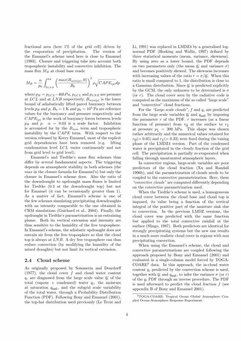
fractional area (here 1% of the grid cell) driven bythe evaporation of precipitation. The version ofthe Emanuel’s scheme used here is close to Emanuel(1993). Closure and triggering take into account bothtropospheric instability and convective inhibition. Themass flux MB at cloud base reads:

MB =α

p0

∫ pB

pLNB

(

max(Bmin(p), 0)

B0

)2

ρ√

CAPE(p)dp

where pB = pLCL−40hPa, pLCL and pLNB are pressureat LCL and at LNB respectively, Bmin(p) is the lowerbound of adiabatically lifted parcel buoyancy betweenlevels pB and p, B0 = 1 K and p0 = 105 Pa are referencevalues for the buoyancy and pressure respectively andCAPE(p) is the work of buoyancy forces between levelspB and p. α = 0.03 is a scale factor. Inhibitionis accounted for by the Bmin term and troposphericinstability by the CAPE term. With respect to theversion released by Kerry Emanuel, most of the explicitgrid dependencies have been removed (e.g. liftingcondensation level LCL varies continuously and notfrom grid level to grid level).

Emanuel’s and Tiedtke’s mass flux schemes thusdiffer by several fundamental aspects. The triggeringdepends on atmospheric stability in both schemes (themax in the closure formula for Emanuel’s) but only theclosure in Emanuel’s scheme does. Also the ratio ofthe downdraught to updraught mass fluxes is limitedfor Tiedtke (0.3 at the downdraught top) but notfor Emanuel (it can be occasionally greater than 1).As a matter of fact, Emanuel’s scheme is one ofthe few schemes simulating precipitating downdraughtswith an intensity comparable to the one obtained inCRM simulations (Guichard et al., 2004). Finally, theupdraught in Tiedtke’s parametrization is an entrainingplume. Both its vertical extension and intensity arethus sensitive to the humidity of the free troposphere.In Emanuel’s scheme, the adiabatic updraught does notentrain air from the free troposphere so that the cloudtop is always at LNB. A dry free troposphere can thusreduce convection (by modifying the humidity of themixed draughts) but not limit its vertical extension.

2.4 Cloud scheme

As originally proposed by Sommeria and Deardorff(1977), the cloud cover f and cloud water contentqc are diagnosed from the large scale value qt of thetotal (vapour + condensed) water qt, the moistureat saturation qsat, and the subgrid scale variabilityof the total water, through a Probability DistributionFunction (PDF). Following Bony and Emanuel (2001),the top-hat distribution used previously (Le Treut and

Li, 1991) was replaced in LMDZ4 by a generalised log-normal PDF (Hosking and Wallis, 1997) defined bythree statistical moments (mean, variance, skewness).By using zero as a lower bound, the PDF dependson two parameters only (the mean qt and variance σ)and becomes positively skewed. The skewness increaseswith increasing values of the ratio r = σ/qt. When thisratio is small compared to 1, the distribution is close toa Gaussian distribution. Since qt is predicted explicitlyby the GCM, the only unknown to be determined is σ(or r). The cloud cover seen by the radiative code iscomputed as the maximum of the so called “large scale”and “convective” cloud fractions.

For the “Large-scale clouds”, f and qc are predictedfrom the large scale variables qt and qsat by imposingthe parameter r of the PDF. r increases (as a linearfunction of pressure) from r0 at the surface to r1at pressure p1 = 300 hPa. This shape was chosenrather arbitrarily and the numerical values retained forr0(= 0.05) and r1(= 0.33) were fixed during the tuningphase of the LMDZ4 version. Part of the condensedwater is precipitated in the cloudy fraction of the gridcell. The precipitation is partially re-evaporated whenfalling through unsaturated atmospheric layers.

In convective regions, large-scale variables are poorpredictors of the cloud fraction (Xu and Randall1996b), and the parametrization of clouds needs to becoupled to the convective parametrization. Here, these“convective clouds” are computed differently dependingon the convective parametrization used.

When the Tiedtke’s scheme is used, a homogeneouscloud cover between the cloud base and cloud top isimposed, its value being a function of the verticalintegral of the positive part of the moisture sink dueto convection. In the previous LMDZ versions, thecloud cover was predicted with the same functionbut applied to the total convective rainfall at thesurface (Slingo, 1987). Both predictors are identical forstrongly precipitating systems but the new one resultsin a much more realistic cloud cover in regions with nonprecipitating convection.

When using the Emanuel’s scheme, the cloud andconvective parametrizations are coupled following theapproach proposed by Bony and Emanuel (2001) andevaluated in a single-column model forced by TOGA-COARE3 data. In this approach, the in-cloud watercontent qc predicted by the convection scheme is used,together with qt and qsat, to infer the variance σ (or r)of the qt PDF through an inverse procedure. The PDFis used afterward to predict the cloud fraction f (seeappendix B of Bony and Emanuel 2001).

3TOGA-COARE: Tropical Ocean Global Atmosphere Cou-pled Ocean-Atmosphere Response Experiment.

4

Cloud microphysical properties are computed asdescribed in Bony and Emanuel (2001, Table 2 for waterclouds and case ”ICE-OPT” of Table 3 for ice clouds):temperature thresholds (-15◦C and 0◦C) are used topartition the cloud condensate into liquid and frozencloud water mixing ratios; cloud optical thickness iscomputed by using an effective radius of cloud particlesset to a constant value for liquid water clouds (12 µmin the simulations presented here), and decreasing withdecreasing temperature (from 60 to 3.5 µm) for iceclouds (Suzuki et al., 1993; Heymsfield and Platt, 1984).The vertical overlap of cloud layers is assumed to bemaximum-random.

2.5 The boundary layer scheme

The (quite old) boundary layer scheme of the LMDZ3version was kept for LMDZ4 with some adjustmentsand ad-hoc tunings. The vertical turbulent transportis treated as a diffusion. Up-gradient transport of heatin the convective boundary layer is ensured by adding aprescribed counter-gradient of -1 K km−1 to the verticalderivative of potential temperature (Deardorff, 1966).Unstable profiles are prevented using a dry convectiveadjustment. The surface boundary layer is treatedaccording to Louis (1979). Over oceans, the surfaceroughness length is computed following Smith (1988).The ratio between the neutral drag coefficient for heatand momentum is fixed to 0.8, consistently with theratio obtained by Smith (1988) in moderate to highwind speed.

Following Laval et al. (1981), the turbulent eddydiffusivity is computed as

Kz = max

(

l2

∣

∣

∣

∣

∣

∣

∣

∣

∣

∣

∂~V

∂z

∣

∣

∣

∣

∣

∣

∣

∣

∣

∣

√

1−Ri/Ric,Kmin

)

(1)

where the mixing length l is prescribed as l =

l0(p/ps)2 with l0 =35 m, Ri = g

θ∂θ∂z/∣

∣

∣

∣

∣

∣

∂~V∂z

∣

∣

∣

∣

∣

∣

2

is the

local Richardson number and Ric(=0.4) is a criticalRichardson number. Over continents and ice, thevalue of the minimum diffusivity, Kmin=10−7 m2 s−1,was tuned in order to get the right strength for thepolar inversion (Krinner et al., 1997; Braconnot, 1998;Grenier et al., 2000). Over oceans, in order to obtaina satisfactory contrast between trade wind cumuliand strato-cumuli on the eastern borders of basins, adiffusion coefficient Kz is first computed with a verysmall minimum diffusivity Kmin=10−10 m2 s−1, whichtends to produce a strong overestimate of boundarylayer cloud coverage over the oceans (Grenier, personalcommunication). A second ad-hoc (and generallystronger) diffusivity, Kz = ξl2 with ξ = 0.002 s−1,

is used if the temperature inversion at the boundarylayer top is weak (in practice if the maximum value ofthe vertical gradient of potential temperature, −∂θ/∂p,is larger than 0.02 K/Pa). The first coefficient is mainlyactive in the subsidence regions, especially on the Eastside of oceanic basins. The second one produces smaller(in fact too small) cloud covers in regions of trade windcumuli.

2.6 Surface processes

For coupling purposes, a fractional land-sea mask isintroduced in the model. Each grid cell is divided into4 sub-surfaces corresponding to continental surface,free ocean, sea-ice and ice-sheet. Surface fluxes arecomputed using parameters (roughness length, albedo,temperature, humidity etc..) adapted to each surfacetype. For each atmospheric column, vertical diffusionis applied independently for each subsurface, and theresulting tendencies are averaged. An interface modelis introduced which separates surface and atmosphericprocesses. The calculation of surface fluxes is donein an independent model, to which the sensitivities ofthe fluxes to temperature have to be provided in orderto preserve the properties of the implicit scheme asdescribed by Dufresne and Grandpeix (1996) and Martiet al. (2005). With this formulation the flux model canbe either a routine in the atmospheric model, an oceanmodel or a land surface scheme.

For continental surfaces, thermal conduction is com-puted with a 11-layer model following Hourdin et al.(1993). The bucket model used in previous versionsto compute soil moisture and evaporation4 is replacedin LMDZ4 by the two-layer hydrological scheme (in-spired from Jacquart and Choisnel, 1995) of the OR-CHIDEE surface-vegetation-atmosphere transfer anddynamic vegetation model (de Rosnay et al., 2002;Krinner et al., 2005). Computation of the evapo-transpiration depends on the plant functional type.Seasonally varying plant leaf area index is prescribedafter satellite data (Myneni et al., 2002). Details aregiven by Krinner et al. (2005). Note that a numericalproblem in the surface scheme was identified after therealisation of the IPCC simulations. It produces occa-sionally very cold temperatures over one time-step invery dry continental regions in the tropics. Although amore robust and improved version of this surface model

4In the bucket model, the soil water content is described asa single reservoir height h which evolves according to the netwater budget P−E (Precipitation minus Evaporation); E = βEp,where Ep is the potential evaporation (that of a free surface ofwater) and β = min(1, h/hp) with hp = 75 mm. Water in excessof the maximum content (hmax = 150 mm) is lost through run-off.

5

is now available, the same version as for the IPCC sim-ulations is used here, on purpose.

3 Basic elements of model clima-

tology

In this section, we present elements of climatology ofthe LMDZ4 model using simulations which follow theprotocol of the Atmospheric Model IntercomparisonProject (AMIP, see Gates, 1992)5. An ensemble of5 AMIP simulations covering the 1979-2002 periodhas been performed. Each simulation differs from theothers only by the initial state of the atmosphere,which is issued from 5 different 1st January of aprevious AMIP II experiment. The monthly seasurface temperatures and sea-ice boundary conditionsconstructed at PCMDI (Program for Climate ModelDiagnosis and Intercomparison) (Taylor et al., 2000)are first interpolated on the LMDZ grid and then todaily values using cubic-splines.

3.1 Mean meridional structure

Fig. 1 presents, in latitude/pressure coordinates, thezonally averaged zonal wind, temperature and relativehumidity for mean January and July conditions (greyscales). The thick superimposed contours show thedifference with the European Re-Analysis (ERA40) ofECMWF for the same period.

First, and contrary to previous versions of the LMDmodel, LMDZ4 no longer shows a systematic coldbias in the lower troposphere. A significant cold biashowever persists at the tropopause (100-300 hPa) inthe extra-tropics. The model tends to be drier thanERA40 in the ITCZ region and wetter in mid-latitudes,with a maximum difference of about 15% in the roaringforties in July. The intensity of the winter jets isgenerally somewhat overestimated. The summer jetsmaximum intensity is better reproduced. A systematicshift toward the equator can also be seen from thedipolar structure in the difference with ERA40 withpositive difference equatorward and negative differencepoleward of the jet.

To evaluate the cloudiness in terms of cloud typesand cloud properties, we compare the model withthe International Satellite Cloud Climatology Project(Rossow and Schiffer, 1999) ISCCP-D2 data. To

5The AMIP II experimental protocol requirements are allfulfilled for the simulations presented here, except that the modelwas not explicitly spun-up at the beginning of the AMIP period.Instead, each simulation starts from a ”quasi-equilibrium” statecorresponding to a previous AMIP II simulation for which therewas no perceptible trend in deep soil temperature and moisture.

be consistent with observations, we use the so-called“ISCCP simulator” (Klein and Jakob, 1999; Webbet al., 2001) that emulates the satellite view of cloudsusing as inputs the vertical profiles of convective andlarge scale cloud amounts simulated by the model.The model simulates reasonably well the latitudinaldistribution of high clouds, with an overestimate of thehigh thick clouds at mid latitudes (Fig. 2). The thinand medium mid clouds are strongly underestimated.The low thin clouds are underestimated, the mid lowclouds are overestimated at mid and high latitudes,whereas the thick low clouds have a reasonablelatitudinal distribution. The LMDZ model displaysbiases which are common to other GCMs (see e. g.,Zhang et al., 2005).

Additional diagnostics more specific of low, mid orhigh latitudes are detailed below.

3.2 Tropics

Regarding the tropics, we show in Fig. 3 the structureof the rainfall and net cloud radiative forcing.

In January, the model predicts a maximum ofrainfall in the region of the Indonesian oceaniccontinent, in qualitative agreement with observations.The strong maxima simulated on the major islands inthis region are however irrealistic. Over continents,the maximum rainfall is also rather well located with acorrect intensity but with a tendency to ”confine” theprecipitation regions. There is a lack of precipitationover the amazonian delta for January and over Saheland North-West India for July. The rainfall monsoonis also underestimated on the West coast of Indiaand overestimated over the Indian sub-continent. Themaximum over Bay of Bengal has almost the goodintensity but it is shifted to the south when comparedto Xie and Arkin (1997) climatology.

The distribution of the net cloud radiative forcingis compared to the data of the Earth Radiation BudgetExperiment (ERBE, Barkstrom, 1984) on the rightpanels of Fig. 3. The strong positive bias on theWest tropical Pacific Ocean in the winter hemisphereand over Sahara is due to an overestimate of thelongwave radiative forcing by high clouds. The negativeradiative forcing is also not strong enough over theregions of tropical rainfall on continents, due to anunderestimate of the shortwave cloud radiative forcing.However, this bias is partly explained over SouthAmerica by the underestimate of the convective activityitself (and associated rainfall). One can notice a goodrepresentation of the seasonal cycle of cloud forcing(by strato-cumulus clouds) on the east side of oceanicbasins (with a maximum in local summer) and a good

6

Figure 1: Zonally averaged temperature (T , K), relative humidity (RH, %) and zonal wind (U , m s−1) simulatedfor the AMIP period (grey scale) in January (left) and July (right). The model results are averaged over the 5simulations and for the period 1980-2002. The difference with the ERA40 reanalysis is superimposed with regular(thick) contours (2 K for T, 6% for RH and 2 m s−1 for U).

( 68

0−44

0 hP

a)M

id(

belo

w 6

80 h

Pa)

Low

( ab

ove

440

hPa)

Hig

h

Cirrus Cirro−Stratus Deep Convection

Cumulus

Alto−Cumulus

Strato−cumulus Stratus

Alto−stratus Nimbo−Stratus

Thick ( 23 < )Medium ( 3.6 < < 23 )τ τThin ( < 3.6)τ

Figure 2: Zonal and annual mean of the nine ISCCP cloud types issued from the ISCCP-D2 satellite data (dashed)and simulated (full curves) by the LMDZ control run. The nine ISCCP cloud types are defined by three bins ofcloud-top pressures (displayed on the left) and three bins of optical thickness τ .

7

January

July

Figure 3: Averaged precipitation (mm/d) and net cloud radiative forcing (W m−2) for the ensemble mean of theAMIP simulations over the period 1980-2002 and for the Xie and Arkin (1997) and ERBE observations.

8

longitudinal contrast over oceans (especially for thesummer hemisphere).

3.3 Mid latitudes

Steady and transient planetary waves

For conciseness, and because the variability is largestduring winter, we show results for December-January-February in the Northern Hemisphere and June-July-August in the Southern Hemisphere.

For the Northern Hemisphere, the averaged geopo-tential at 700 hPa, Z700 (Fig. 4, panels a), presentstwo major troughs at the east coasts of America andAsia, and two major ridges over Northeastern Americaand Northeastern Europe. There is a less pronouncedtrough over Central Europe and a weak ridge to its East(i.e. to the North of the Himalayan plateau). Thesefeatures are well predicted in the model (left side ofFig. 4) when compared to the reanalysis (right side).This, in part, results from the action at low level of theSubgrid Scale Orographic scheme (Lott, 1999). Themodel however slightly overestimates the ridge over theRockies but underestimates the difluence of the jet overwestern Europe. The systematic shift of the simulatedjets toward the equator is also visible on those maps.

The Root Mean Square (RMS) of Z700 (Fig 4)reveals two centres of action, slightly to the west ofthe two major ridges in Fig. 4a. The location of thesetwo centres of action is realistic when compared toreanalysis. The model nevertheless seems to slightlyoverestimate the tropospheric variability over the Northeastern Pacific. As the total variance in the atmosphereis dominated by the low-frequency variability (Sawyer,1976; Blackmon, 1976), the RMS fields in (panels b)hide the transient eddies resulting from the baroclinicinstabilities generated where the mid-latitude jet isintense (on the lee side of the two major troughsin panels a). To isolate these baroclinic eddies, wenext use the procedure of Hoskins et al. (1996) anddefine the high pass transient fields by the differencebetween the daily field and the centred box-car 3–day mean of that field. The RMS of this high passfield (Fig. 4c) shows baroclinic storm tracks locatedat the two jet exits, with maximum variance over thewestern half of the two oceans and extension over theentire oceanic basins. Note nevertheless that the modelunderestimates substantially the high pass RMS overthe entire Pacific.

For the Southern Hemisphere winter, the climato-logical mean flow (Fig. 4d) is much more zonal. Around60oS, it presents enhanced variance over nearly half theglobe, with a maximum over southern east Pacific nearthe Drake passage (Fig. 4e). The pattern of high fre-

quency in Fig. 4f presents enhanced variance slightly tothe north of the maximum of total variance in Fig. 4e.It covers more than half the globe around 50oS. Again,these patterns are rather realistic, with the model over-estimating the total variance and underestimating thehigh pass variance.

Interannual variability

A large number of spatial patterns and indices hasemerged in studies of the northern hemisphere winter-time extra-tropical variability. Recently, Quadrelli andWallace (2004) have shown that they can all be almostfully retrieved by a linear combination of only two basispatterns: the leading two Empirical Orthogonal Func-tions (EOF) computed by a principal component analy-sis of the monthly sea level pressure (SLP) field. EOF1of the ERA40 SLP for the 1980-2001 period (Fig. 5) is aquasi-zonally symmetric dipole between the polar andmid-latitudes also called the Northern Annular Modeor Arctic Oscillation (Thompson and Wallace, 1998).EOF2 is a wavy pattern with a large centre of actionover the Pacific and a weaker secondary wave train overEurope. The two EOFs are orthogonal by construction.

Following Quadrelli and Wallace (2004), the first2 EOF of each simulation are projected on the twobasis patterns. In the right panel of Fig. 5, eachEOF is represented by a line whose projections on thehorizontal and vertical axes give the correlation withthe basis EOF 1 and 2, respectively. The lines gatheraround the two axes with a spread indicative of thevariability between different simulations. An ensembleEOF, computed from all experiments together, is alsoshown. The simulated patterns of variability correlatevery well with the observed basis functions, particularlyfor EOF1 which is the larger scale pattern.

3.4 High latitudes

In polar region, the climate is often rather poorlyrepresented in global models (Chen et al., 1995). Thedata are also scarce and the quality of gridded datasetsoften remains questionable. Here we compare modeloutput to station measurements over the relativelyuniform plateau regions in the centre of the ice sheets.Fig. 6 shows the simulated (but altitude-correctedfollowing Krinner and Genthon (1999)) and observed(Automatic Weather Stations Project, 2004; AutomaticWeather Stations Greenland Project, 2004) monthlymean surface air temperatures at Summit (CentralGreenland) and Dome C (Central East Antarctica).The model reproduces rather correctly the observationsapart from a cool bias at Summit. This coolbias is probably caused by an underestimate of the

9

SH, JJANH, DJF SH, JJANH, DJF

Hig

h pa

ss R

MS

Tot

al R

MS

Mea

n

LMDZ4 (AMIP) ECMWF

Figure 4: Winter statistics of 700hPa geopotential height for 20 winters and from the LMDZ4 model (left side) andERA40 ECMWF analysis (right side) for the the Northern Hemisphere in December-January-February (NH, DJF)and for the Southern Hemisphere in June-July-August (SH, JJA). (a)-(d) winter mean, contour interval 50m; (b)-(e)RMS, contour interval 10m; (c)-(f) RMS high pass, contour interval 5m

EOF 2EOF 1

EOF1

EO

F2

AM

IP E

NS

2

AMIP ENS 1

Figure 5: Leading 2 EOF of monthly wintertime northern hemisphere SLP, 1980-2001 (Contours every 1hPa) andprojections (area-weighted correlations) of the EOF of the different simulations on the phase space defined by thetwo EOFs. For reference, a circle of radius unity is plotted. Thin lines are individual simulations, the thick lines arefor the ensemble.

10

Summit, Central Greenland

Dome C, Central East Antarctica

Figure 6: Monthly mean surface air temperatures atSummit (38◦W, 72◦N, 3250 m asl) and Dome C (123◦E,75◦S, 3300 m asl) as simulated with LMDZ4 (full curve,AMIP simulation) and observed (dashed).

downwelling longwave radiation, a relatively frequentmodel bias over ice sheets (e.g., King and Connolley,1997). In Antarctica, the smaller bias probably comesfrom an error compensation. As noted by Krinner et al.(1997), the orographic roughness calculated from thesubgrid variability of surface altitude is often too high(as is the case here) over the ice sheet escarpments,which are in reality smooth sloping surfaces. It leadsto an underestimate of the surface wind speed over thecontinent margins and of the intensity of the Antarctickatabatic drainage flow in general (James, 1989).Sensitivity tests with strongly decreased orographicroughness have shown strongly increased, and morerealistic, surface wind speeds in Antarctica, but astrong cooling (about 5◦C) over the continent.

In the two polar sites considered here, with rareblowing snow and no melt, the surface mass balance iseasy to measure through shallow firn cores and is simplythe difference between precipitation and sublimation.Surface mass balance at Dome C is 25 kg m−2 per year(EPICA community members, 2004); at Summit, it isapproximately 220 kg m−2 per year (Shuman et al.,

1995). The corresponding values for LMDZ4 are 43kg m−2 per year for Dome C and 146 kg m−2 per yearfor Summit. High resolution (60 km) simulations overAntarctica with a zoomed version of the same model(Krinner et al., submitted) yield a surface mass balanceof 31 kg m−2 per year at Dome C, which is closer tothe observed value.

Over Antarctica as a whole, the average simulatedprecipitation minus sublimation for Antarctica is 184kg m−2 per year, which is not far from the currentbest estimate of surface mass balance of 166 kg m−2

per year (Vaughan et al., 1999). Over the Arcticbasin, available gridded precipitation maps (ArcticClimatology Project, 2000) suggest a wet bias (about25 to 50%) of the model.

4 Sensitivity to parametrized

physics

4.1 Sensitivity experiments

A series of sensitivity experiments were conducted byreplacing one element or parameter of the reference ver-sion. All the sensitivity experiments use climatologicalSSTs (no interannual variations) corresponding to themean seasonal cycle of the AMIP boundary conditions.The simulations are performed over 7 years, the last 6of which are retained for analysis. The following simu-lations are considered here:

1. CONTROL: Same model version as for AMIPsimulations but with climatological SSTs. Usedas a control for the sensitivity experiments.

2. TIEDTKE: The convection scheme is switchedfrom Emanuel’s to Tiedtke’s. The radiativeimpact of convective clouds is also treateddifferently as explained above. Both theCONTROL and TIEDTKE simulations are inglobal radiative balance with a difference of lessthan 1 W m−2.

3. CLOUDSA: The coupling between the convectionscheme and cloud schemes (Bony and Emanuel,2001) is NOT activated.

4. CLOUDSB: Same as CLOUDSA but with a widerPDF for subgrid-scale water (r1 and r0 multipliedby 2 with respect to CLOUDSA). This case isused here to show the impact on the large scalecirculation of the radiation tuning and to helpanalysing the other sensitivity experiments. Interms of the accuracy of the cloud radiativeforcing representation, this simulation is not so far

11

Figure 7: Impact of the convection (TIEDTKE,top) and cloud scheme (CLOUDSB, bottom) on theJanuary mean temperature (left, difference betweenthe sensitivity run and CONTROL) and humidity(right, relative difference between the sensitivity runand CONTROL in %). We use log pressure on thevertical in order to focus on the tropopause level. Theshaded area correspond to a colder (left) and wetter(right) atmosphere in the sensitivity experiment.

from what was typically at work in the previousgeneration of climate models (e. g. Bony et al.,2004).

5. BUCKET: The bucket scheme is activated inplace of ORCHIDEE for the surface hydrology.

An additional simulation (HIGHRES) is performedwith the same version of the model as for CONTROLbut with a finer horizontal resolution of 1.876◦ by 1.25◦.

4.2 Mean meridional structure

The magnitude of the cold bias of the mid and highlatitude tropopause (100-300 hPa) is sensitive to boththe convection and cloud schemes. The bias is abouttwice as strong in the TIEDTKE simulation as in theCONTROL (typically -8 K instead of -4 K) in thesummer (southern) hemisphere (upper left panel inFig. 7). On the contrary the CLOUDSB simulationis globally much warmer at the tropopause in theextra-tropics (lower left panel), and even shows aslight warm bias there. In both cases, the differencein temperature is directly related to the humiditychange shown in the right panels. At the modeltropopause indeed, the radiation alone almost balancesthe large scale dynamical tendency. The optically thin

approximation is also valid so that, in the absenceof temperature change, a larger humidity results in alarger cooling to space. For the two cases discussedhere, it can be shown that this radiative effect is directlyresponsible for the modification of the temperature atthe tropopause. More precisely, the atmosphere cools(TIEDTKE) or warms (CLOUDSB) until radiationbalances the dynamical large scale tendency which isnot strongly affected (not shown).

For TIEDTKE, the additional humidity comesdirectly from a small but systematic import of water bydetrainment, due to a so-called ”mid-level” convection.This additional convection is active above the mainconvection which peaks well bellow 300 hPa in mid andhigh latitudes.

For CLOUDSB, when increasing the width ofthe PDF6, large scale clouds appear and precipitatewell before reaching large scale saturation, whichexplains the drier atmosphere. Note also that,because of the weaker atmospheric extinction, thelongwave radiation escapes more easily from the lowertroposphere resulting in a colder atmosphere there.

For all the runs presented here, the zonally averagedrainfall (upper panels of Fig. 8) is overestimatedbetween 40 and 70◦S for all seasons and underestimatedin the southern tropical band in January, whencompared to Xie and Arkin (1997) climatology. Notealso, for January, an underestimate of the rainfallat 10◦S, corresponding to an underestimate of theSouth Pacific Convergence Zone. In the TIEDTKEsimulation, the rainfall is even slightly stronger at10◦N than at 10◦S. The introduction of the Orchideescheme in place of the old bucket scheme (CONTROLsimulation versus BUCKET) for soil moisture resultsin a decrease of summer rainfall in the mid latitudesover continents, in better agreement with observationsas seen in the upper right panel of Fig. 8 (40-70◦N).

As stated above, particular care was given tothe tuning of the cloud radiative forcing, andin particular to its latitudinal variations. Theoverall agreement with ERBE observations (Barkstrom,1984) is good, especially in the tropics (intermediatepanels in Fig. 8). The CLOUDSA simulation hasa weaker (less negative and farther from ERBEobservation) shortwave radiative forcing in the tropics.Beyond physical consistency, this is the main reasonwhy the Bony and Emanuel (2001) approach wasadopted. The CLOUDSB simulation shows a very goodrepresentation of the net cloud radiative forcing in thetropics, but this is due to a compensation betweenforcings that are too weak in both the longwave and

6The difference is the same when comparing CLOUDSB withCLOUDSA or CONTROL simulations.

12

January July

Figure 8: Zonally averaged rainfall (mm d−1);shortwave (SW), longwave (LW) and net (NET) cloudradiative forcing (CRF, W m−2); and wind stress overthe ocean (N m−2). Superimposed to observations(grey), we show the AMIP results (+), the CONTROLsimulation (×, often superimposed) and results ofthe sensitivity experiments (thin curves). For clarity,each graph only considers a relevant subset of thoseexperiments. Observations are from Xie and Arkin(1997) for rainfall, from ERBE for radiation and fromERS for surface drags.

shortwave radiation.The surface stress (lower panels in Fig. 8) is

also a very important quantity for the coupling withoceans. The zonally averaged zonal stress associatedwith trade winds (local minima around 20◦N and20◦S) are well simulated for the AMIP and CONTROLsimulations when compared to ERS scatterometer data,and slightly too strong for TIEDTKE. The latitudinalshift of the mid-latitude jets is clearly visible on thosecurves as well as the strong positive impact of anincrease of the horizontal resolution (HIGHRES) inthat respect.

The finer grid has impact on other aspects of theclimatology. The high frequency variability in mid-latitudes is for instance much better represented. Atthe same time, the tendency of the model to confinethe tropical precipitations over continents is reinforced.The interpretation of those results is out of the scopeof this paper and will not be discussed here.

4.3 Hadley-Walker circulation

The large scale distribution of tropical rainfall displaysimportant differences between the sensitivity runs.These changes are usually difficult to interpret becausethey are often dominated by localised patterns or smallshifts in the spatial structure. However, those changesare associated with large scale circulation changes.These changes will be described in this section and willbe interpreted in the following one.

Method of analysis

In order to characterize the tropical large scalecirculation in the tropics in the various sensitivityexperiments, we first consider the scalar potential ϕ200

of the horizontal wind at 200 hPa. The scalar potentialis defined from the decomposition of the horizontalvelocity ~V into its divergent and rotational parts as

~V = ~∇ϕ+ ~∇∧ ~ψ (2)

This potential will be called velocity potential ϕ. ItsLaplacian is also the wind divergence

~∇.~V = ∇2ϕ (3)

A local minimum of the velocity potential at 200 hPacorresponds to a horizontal divergence and is generallyassociated to a large scale ascent in the atmosphericcolumn. This pressure level is generally retained foranalysis because the divergence is generally maximumthere. This is true on average, but a divergence below200 hPa can be missed in the velocity potential even fora strong ascent but confined to lower pressures. In order

13

ϕ200 ϕ

Figure 9: Velocity potential of the wind at 200 hPa (ϕ200, left, unit 106 m2 s−1) and of the z-weighted potential (ϕ,

right, unit 1015 W); annual mean for the 1980-2002 period for ERA40 and for a 6-year average for CONTROL andTIEDTKE simulations.

to overcome this problem, we consider also the scalarpotential ϕ associated with the vertically integratedhorizontal transport of geopotential

∫ ps

0dp ~V gz. This

potential is close to a z-weighted integral of the velocitypotential (see Appendix A)

ϕ '

∫ ps

0

dp z ϕ (4)

It will be called z-weighted potential hereafter. It isalso shown in Appendix A that

w '1

g∇

2ϕ (5)

where w is the total vertical momentum of theatmospheric column

w =

∫ ∞

0

dz ρ w ' −

∫ ∞

0

dzω

g(6)

where w and ω are the vertical velocity expressed in zand pressure coordinate respectively.

Annual mean potentials

In the reanalysis, the overall structure of the velocitypotential at 200 hPa, ϕ200, is characterized by astrong minimum (maximum ascending motion) over thewestern equatorial Pacific (upper left panel in Fig. 9).Secondary minima, associated with the tropical forests

ϕ200

Figure 10: Velocity potential at 200 hPa (ϕ200,unit 106 m2 s−1); annual mean for a 6-year averagefor CLOUDSA, CLOUDSB and BUCKET sensitivityexperiments.

14

over Africa and Amazonia are also visible as well as themaxima associated with dry subsiding regions on theeastern side of the tropical Atlantic and Pacific oceans.

This structure is reproduced reasonably well in theCONTROL simulation. Among the main differences,one can note that the trough of the equatorial EastPacific is not as marked as in the reanalysis. Theminimum over Amazonia is also somewhat moreconfined and shifted toward central America thanin the reanalysis. More quantitatively, one maynotice that the velocity potential variation between itsminimum on the West and local maximum on the Eastequatorial Pacific is about 30% larger in the CONTROLsimulation. In comparison, the structure of ϕ200 in theTIEDTKE simulation shows significant differences, themost noticeable being the quasi disappearance of thevelocity potential minimum over Africa and the shiftof the Amazonia minimum towards the equatorial EastPacific.

As expected, the z-weighted potential ϕ maps (rightpanels of Fig. 9) are quite similar to the velocitypotential ϕ200 ones. In the CONTROL simulation,most of the comments made from the velocity potentialϕ200 remain true, except for the total variation ofϕ over the equatorial Pacific which is quite close inCONTROL and ERA40. This remarks also holds forthe contrast between the local minimum over EastAfrica and local maximum over South Atlantic. For theTIEDTKE simulation, the ϕ field is closer to ERA40over continents (some z-weighted potential trough ispresent over East Africa while absent in ϕ200 field) butfarther over ocean (a strong trough is associated to theITCZ over the eastern equatorial Pacific).

The two potentials ϕ and ϕ200 considered togetheryield indications about the vertical distribution ofvertical velocity. In particular, the fact that the localminima over continents are overmarked in ϕ200 but notin ϕ for the CONTROL simulation is indicative of largescale vertical (upward) velocities peaking higher, witha larger wind divergence at 200 hPa than in the re-analysis. The same comparison of ϕ and ϕ200 for theTIEDTKE simulation suggests a relatively lower heightfor the large scale ascent over Amazonia and Africathan in the re-analysis.

For the CLOUDSA experiment (Fig. 10), the ϕ200

minima over Africa and Amazonia are deeper than inthe CONTROL. It is the opposite for CLOUDSB whichtends to mimic the relative weakness of continentalascent in TIEDTKE. The ϕ fields are in fact veryclose to each other over Africa and Amazonia for theCLOUDSB (not shown) and TIEDTKE simulations.However, the associated minima in ϕ200 still appearfor CLOUDSB while they are absent for TIEDTKE.

This suggests that the cloud scheme change affects thestrength of the large scale ascent, but not its height,whereas the use of the Tiedtke’s scheme in place ofthe Emanuel’s both affect the strength of the ascendingmotions over continents and the vertical profile of thevertical velocity.

Finally, the BUCKET simulation is not verydifferent from CONTROL with possibly a betterrepresentation of the large scale ascent over Amazoniabut a worse representation of the African trough whichis shifted to the East.

Potential and rainfall

The changes analysed above have significant signaturein terms of seasonal rainfall. In January, threeof the sensitivity runs (TIEDTKE, CLOUDSB andBUCKET) show a similar and unrealistic maximumof precipitation North-East of Madagascar (Fig. 11,left). This feature is related to a weakening of thelarge scale ascent over Indonesia (positive differenceFig. 11. right) associated with a weakening of theWalker circulation across the Indian Ocean. In July,a similar weakening of continental ascent in TIEDTKEsimulation is associated with a longitudinal structureof wave number 1 (Fig. 12) in the difference of the z-weighted potentials. The large scale ascent is globallyweakened in the 0-160E longitude band, and monsoonrainfall are less abundant over the Indian and Africancontinents. For India itself, this can be considered asan improvement with respect to CONTROL simulationwhich produces too much rain over the continent andnot enough on the West coast.

The Tiedtke’s scheme also tends to produce narrowand strong rainfall patterns over oceans. This isespecially the case over East Pacific (Fig. 11 and 12)where it is associated with a strong trough in the annualmean velocity potentials ϕ200 and ϕ (Fig. 9).

4.4 Regime sorted analyses

So far, we have analysed how the different parametriza-tions affect the large scale Hadley-Walker circulationand the distribution of rainfall. In this section, we tryto relate these modifications to the intrinsic behaviourof the parametrizations.

The heating and moistening effect of eachparametrization on the atmospheric environment(which corresponds in GCMs to diabatic tendencies oftemperature and moisture) depends to a large extenton the large-scale atmospheric circulation in which itis embedded. As the geographical distribution and theintensity of large-scale dynamical patterns generally dif-fer between simulations (as well as between models and

15

Figure 11: January rainfall (left, mm d−1) and z-weighted potential ϕ (right, unit 1015 W) for the CONTROLand sensitivity experiments. For the sensitivity experiments, the right panel is the difference of ϕ with that of theCONTROL simulation with same units.

Figure 12: Same as Fig. 11 but for July and CONTROL and TIEDTKE.

16

−100 −80 −60 −40 −20 0 20 40 60 800

0.02

0.04

0.06

0.08

0.1

0.12

PD

F

Obs maxObs minCONTROLCLOUDSACLOUDSBTIEDTKE

ω500 (hPa d−1)

Figure 13: Probability distribution function of ω500 inthe 30S-30N latitude band over oceans for two setsof reanalysis (ERA40 and NCEP2 giving rise to thegrey area) and for the CONTROL, CLOUDSA/B andTIEDTKE experiments.

observations), it is difficult to analyse and to comparethe behaviour of parametrizations by considering onlyhorizontal maps or zonal averages.

To make this comparison easier and to get somedeeper insight in how the different schemes work,we adopt the compositing methodology proposed byBony et al. (1997) which uses the large-scale monthly-mean mid-tropospheric (500 hPa) vertical pressurevelocity ω as a proxy for large-scale rising (ω < 0)or sinking (ω > 0) motions. As shown by Bonyet al. (1997), and illustrated further below, this methodallows to classify the tropical regions according totheir convective activity, and to segregate in particularregimes of deep convection from regimes of shallowconvection.7

This methodology, previously applied to cloudfeedback studies (Bony et al., 2004; Bony and Dufresne,2005; Wyant et al., 2005), is used here to study thebehaviour of different parametrizations in the Tropics.Following those previous studies, we keep ω500 as aproxy although ∇2ϕ is a promising alternative (seeAppendix A). The regime sorting is applied tomonthly outputs of a 6 years long simulation (i. e.72 monthly means) for the 30◦S-30◦N region. Givena bin K in vertical velocity, of central value ωK

and width δω (here 5 hPa/d), and for each modelvariable X, the regime sorted value reads XK =∑

(i,m)∈WkaiX(i,m)/

∑

(i,m)∈WKai where WK is the

ensemble of pairs of grid indices i and months m, forwhich ωK − δω/2 < ω500(i,m) ≤ ωK + δω/2 and ai isthe area of mesh i.

7In the tropics, nearly all of the upward motion associatedwith ensemble-average ascent occurs within cumulus clouds,and gentle subsidence occurs in-between clouds. The rate ofsubsidence in-between clouds being strongly constrained by theclear-sky radiative cooling (which is nearly invariant), an increaseof the large-scale mean ascent corresponds, to first order, to anincrease of the mass flux in cumulus clouds (Emanuel et al. 1994).

Figure 14: Convective heating rate (K d−1) in aregime sorted diagram (pressure in hPa versus ω500 inhPa d−1) for the CONTROL (with Emanuel’s scheme)and TIEDTKE experiments over oceans (left) andcontinents (right). Note that the contouring is refinedaround 0.

When comparing different parametrizations in thisframework, one must keep in mind the underlyingprobability distribution function which gives therelative weight of the various regimes. The PDF itselfis indeed sensitive to parametrization changes (Fig. 13).When compared to the ERA40 and NCEP re-analysisor to the TIEDTKE simulation, the CONTROLsimulation with Emanuel’s convection scheme seems tooverestimate the frequency of the moderate convectiveregimes (-60 < ω500 < -20 hPa/d) and underestimatethe very strong convective regimes. Changes in therepresentation of large scale clouds (CLOUDSB versusCLOUDSA or CONTROL) affects more the PDF insubsidence regimes.

Convection

In order to compare the convective parametrizations(CONTROL versus TIEDTKE), we shall use a series ofregime-sorted versus pressure graphs of the convectiveheating rate, convective moistening, relative humidity

17

Figure 15: Scatter plot of the convective heating rate(K d−1) at the 550 hPa pressure level, as a function ofω500 (hPa d−1).

and cloud cover.First we consider the general features of these

graphs. Fig. 14 displays the convective heating rateω500-pressure graphs. In consistency with the abovediscussion of the link between large-scale verticalvelocity ω and convective activity, we see thatthe behaviour of convective tendencies and of theatmospheric state is very contrasted between deepconvective regimes (ω500 < 0) and shallow convectiveregimes (ω500 > 0). The difference between continentsand oceans is also well marked with, for instance,a cooling by downdraughts in a very shallow layerclose to the surface over the ocean and in a muchthicker layer over land. The heating rate by convectionincreases less rapidly as a function of −ω500 overcontinents because there is less water available there.This contrasted behaviour is further illustrated by ascatter plot (Fig. 15) showing the same heating ratesas in Fig. 14 but for the 550 hPa pressure level. Each

Figure 16: Convective moistening (g kg−1 d−1) withsame conventions as in Fig. 14. Note that thecontouring is refined around 0.

point on these graphs corresponds to one point of thehorizontal grid and one of the 6×12 months of thesimulation used to produce the regime sorted analyses.Note the relatively weak dispersion around the mean,especially for intermediate regimes (-50 hPa d−1<ω500 < 0) over oceans. This is consistent with thepicture of a quasi-equilibrium between convection andlarge scale dynamics in the tropics.

The convective moistening (Fig. 16) is also verycontrasted between deep convective regimes (ω500 < 0),where the parametrization essentially dries the wholeatmosphere by precipitating water onto the ground, andshallow convective regimes (ω500 > 0), where the wateris transported from the surface up to the 850-500 hPapressure range over oceans (with a similar but weakereffect on continents). Near the surface and for allregimes, the (dominant) effect of downdraughts resultsfrom the combination of moistening (and cooling) byevaporation of the falling precipitation and drying(and heating) by downward advection. On continents,because of the relatively weak relative humidity (seeFig. 17), a large part of the precipitation evaporatesin the boundary layer, explaining the weak drying andstrong cooling there. Over ocean, the near saturated

18

Figure 17: Relative humidity (%) with same conven-tions as in Fig. 14.

boundary layer inhibits evaporation and the strongstratification in humidity leads to stronger positivedrying and heating by downward advection.

Turning to the comparison of the two convectiveschemes, the vertical distribution of convective heating(Fig. 14) appears quite different. The Tiedtke’s schemeproduces a deeper convective heating over oceans thanEmanuel’s, with a peak at 550 hPa. Over continent,the convective heating is more homogeneous on thevertical with Emanuel’s, corresponding to a strongerheating above 500 hPa. This is consistent withthe fact that the marked local minima of ϕ200 inthe CONTROL simulation over Africa and Amazonia(Fig. 9) have almost no counterpart in TIEDTKE,while both simulations show similar troughs in the sameregions for the z-weighted potential ϕ. The convectiveheating is altogether significantly stronger and deeperover ocean than over continent with Tiedtke’s while itis somewhat weaker and shallower over ocean than overcontinent when using Emanuel’s scheme.

Another major difference is the much stronger nearsurface cooling with the Emanuel’s scheme. This strongcooling arises from reevaporation of convective rainfallin the unsaturated atmosphere, below the cloud base.This point is further illustrated by a scatter plot of

Figure 18: Cloud cover (%) with same conventions asin Fig. 14.

Figure 19: Scatter plot of the convective heatingrate at the lowest model level and of the surfaceprecipitation over ocean (left) and continent (right)for the Tiedtke’s scheme (light grey crosses), and forthe Emanuel’s scheme (dark grey: no selection, black:ω500 > 20 hPa).

19

the near surface convective heating rate versus surfacerainfall in Fig. 19. Over oceans, the near surface coolingincreases rapidly as a function of precipitation for theEmanuel’s scheme, with a weak dispersion. The coolingalso increases with precipitation for Tiedtke but withmuch smaller values (typically 0.5 instead of 5 K/dayfor Emanuel for a monthly mean precipitation of 10mm/d).

This cooling associated with convective precipita-tions is the main mechanism by which convection sta-bilizes the troposphere (Emanuel et al., 1994). InEmanuel’s scheme the closure is a function of the tropo-spheric stability, which, combined with the near surfacecooling, results in a strong self-inhibition of convection.This self inhibition is responsible for the larger occur-rence of moderate convective regimes (-60 < ω500 < -20hPa/d, Fig. 13), and for the limitation of the convec-tive rainfall and heating rate at 500 hPa visible on thescatter plots (Fig. 19 and Fig. 15 respectively).

With Tiedtke’s scheme, the moisture convergenceclosure does not provide any sensitivity to theatmospheric stability. Some self-inhibition couldhowever be at work since triggering depends on theatmospheric stability, but the stabilization by re-evaporation is too weak. The signature of the absenceof self-inhibition is visible in the tail of the PDF instrong convective regimes (Fig. 13), and in the verylarge values reached by convective rainfall (Fig. 19).Note also that the dispersion of heating rates aroundthe mean (Fig. 15) is particularly weak over oceansfor the Tiedtke’s scheme. This weak dispersion ispresumably mainly a consequence of the closure inmoisture convergence of this scheme which does notleave many degrees of freedom for the parametrizationover the ocean, where humidity is close to saturation,and the convergence of mass is strongly correlated toω500. This correlation together with the absence of selfinhibition explains the boundless linear increase of theheating rate as a function of ω500.

These features of the Tiedtke’s scheme relateto commonly admitted statements about convectiveparametrizations. (i) A strong high frequencyvariability is often attributed to moisture convergenceclosures, whereas small high frequency variability seemsto be a rather general feature of quasi-equilibrium mass-flux schemes (Horinouchi et al., 2003). Consistently,the high frequency variability of tropical rainfall isabout 30 to 50% stronger with Tiedtke’s than withEmanuel’s scheme (not shown). In that respect, theTIEDTKE simulation is much closer to observations.(ii) These features are also closely related to the wave-CISK mechanism described by Lindzen (1974) by whichcoupling between convection and small spatial scale

waves may lead to very localized strong convectiveevents (grid points storms); the absence of evaporativecooling in Lindzen’s model is worth mentioning here.(iii) Finally, these features probably explain theirrealistic patterns of strong rainfall obtained overoceans in the TIEDTKE simulation, over East Pacific(Fig. 11 and 12) all year round and over North-Eastof Madagascar in January (Fig. 11). Very similarpattern are indeed reported in climate simulationsperformed with the ECMWF model, although it uses adifferent closure for the Tiedtke’s scheme which takesinto account atmospheric stability (see e. g. Fig. 12 inJakob and Siebesma, 2003). This apparent insensitivityto closure points to the key role of the lack of nearsurface cooling in Tiedtke’s scheme over oceans.

In the much drier continental air over continents,both schemes yield a similar near surface cooling forprecipitation rates smaller than 3-4 mm/d (left panelin Fig. 19). For higher precipitation rates the cooling isbounded by 3 K/d for Tiedtke’s scheme while it reaches6 K/d with Emanuel’s.

One can notice other differences between the twoconvection schemes. There is a thin layer of coolingaround 100 hPa with the Tiedtke’s scheme which hasno counterpart with the Emanuel’s scheme (Fig. 14).The simulation with the Emanuel’s scheme shows asystematic moistening between 250 and 150 hPa whichis predicted by Tiedtke’s scheme on continents but noton oceans.

In the subsiding regimes over oceans, the nearsurface convective heating is positive in TIEDTKEand negative in the CONTROL simulation. Apartfrom this difference linked to the difference in rainfallevaporation, the heating rate profiles are qualitativelysimilar. They both exhibit a maximum heating of1 K/d around 900 hPa and a small cooling between800 hPa and 550 hPa (smaller with Emanuel’s scheme).

The associated cloud covers are shown in Fig. 18.The fractional cover of mid-level clouds in convectiveregimes is much larger with Tiedtke’s scheme, sincethe cloud cover is imposed as a constant betweencloud basis and cloud top when convection is active.By comparison, the Emanuel’s scheme coupled to theBony and Emanuel (2001) cloud scheme produces lesscloudiness below 500 hPa. In both simulations, thereare very few boundary layer clouds in subsiding regimesover continents.

Clouds

Most of the changes observed in the large scaleorganisation of convection for CLOUDSA and B(Fig. 10) can be explained by looking at cloud radiativeforcing in the regime-sorted framework (Fig. 20).

20

CRFNET CRFLW CRFSW LWTOP NETTOP SWS T2M PRECIP EVAPCONTROL -5.3 51.5 -56.7 -237.0 70.9 225.1 25.6 5.3 4.2

Difference with CONTROLTIEDTKE -13.4 -6.8 -6.7 -8.6 -14.8 -9.5 0.6 1.4 0.6CLOUDSA 7.5 -4.4 11.9 -4.5 6.7 12 -0.1 0 0CLOUDSB -3.5 -18.8 15.2 -24.6 -9.7 15.1 -0.4 0.6 0.4BUCKET -1.4 -2.1 0.5 -1.8 -2.1 -0.4 -0.1 0.2 0.1

Table 1: Net (CRFNET, W m−2), longwave (CRFLW, W m−2) and shortwave (CRFSW, W m−2) cloud radiativeforcing, infrared radiation to space (LWTOP, W m−2), net radiation budget at the top of atmosphere (NETTOP,W m−2), total solar radiation absorbed by the surface (SWS, W m−2), air temperature at 2m above surface(T2M, Celcius), precipitation (PRECIP, mm d−1) and evaporation (EVAP) averaged for convective regimes (-100hPa d−1< ω500 <0) over oceans between 30S and 30N.

CRFNET CRFLW CRFSW LWTOP NETTOP SWS T2M PRECIP EVAPCONTROL 1.6 47.9 -46.3 -241.5 54.0 212.9 24.5 3.9 1.9

Difference with CONTROLTIEDTKE -15.7 -12.3 -3.4 -12.1 -16.5 -6.4 -0.1 -0.5 -0.1CLOUDSA 7.9 1 6.9 0.8 5.9 6 0.1 0.3 0.1CLOUDSB -3.4 -15.6 12.2 -19.7 -10.3 12 -1.1 0 0.1BUCKET -13.5 -2.3 -11.2 0 -9 -9.3 -2 0.7 1.3

Table 2: Same as Table 1 but for continents.

The CONTROL simulation shows reasonable agree-ment with ERBE observations. In subsiding regimes(ω500 > 0), the longwave, shortwave and net compo-nents of the cloud radiative forcings are reasonably closeto the observation on average, when compared for in-stance to the previous generation of models (Bony et al.,2004). For the intermediate regimes, between -30 and0 hPa d−1, the agreement is still good for the longwaveradiative forcing but the shortwave forcing is not neg-ative enough leading to a net negative forcing which isnot strong enough. For strong convective regimes, be-tween -90 and -60 hPa d−1, the good agreement for thenet forcing is due to a compensation of errors betweenthe shortwave and longwave forcing.

The CLOUDSA experiment is very close to CON-TROL in subsiding regimes (as expected). In convec-tive regimes, the activation of the Bony and Emanuel(2001) cloud scheme (CONTROL versus CLOUDSA)reinforces the (negative) shortwave radiative forcing byabout 10-15 W m−2, with almost no effect in the long-wave. Because of the weaker shortwave radiative forc-ing (< 0) in CLOUDSA (with respect to CONTROL)more solar radiation can reach the surface. The meansolar radiation at the surface (SWS) is increased by 12W m−2 on the averaged over the tropical oceans forconvective regimes (Table 1) and by 6 W m−2 overcontinents (Table 2). This increased solar radiation

increases the convection over continents but has almostno effect over ocean (SSTs are fixed) explaining thestronger minima of the velocity potential over Amazo-nia and Centre Africa (Fig. 9 and Fig. 10).

In CLOUDSB, the drier and less cloudy atmosphere(with respect to CONTROL) leads to a larger infraredcooling to space in the lower and mid troposphere.This increased cooling is only partly compensated bythe weaker back-scattering of solar radiation by clouds.Over ocean with fixed SSTs, the larger cooling to spacedestabilizes the atmosphere and increases convection.This increased convection results in a colder near-surface air over the ocean in convective regions (by0.4 K on average, Table 1) despite the imposed SSTs.The same change in radiative forcing produces a coolingof continental surfaces (by about 1.1 K on average in theconvective regimes, Table 2). This in turn explains thereduction of the large scale ascending motions reportedin Fig. 10 and 11.

Similarly, the net radiative forcing is more negativein TIEDTKE simulation than in CONTROL in theconvective regimes, which may also contribute tothe reduction of large scale ascending motions overcontinents (Fig. 9, 11 and 12).

21

−100 −80 −60 −40 −20 0 20 40 60 800

20

40

60

80

100

LW C

RF

(W

/m2)

Obs maxObs minCONTROLCLOUDSACLOUDSBTIEDTKE

−100 −80 −60 −40 −20 0 20 40 60 80−120

−100

−80

−60

−40

−20

0

SW

CR

F (

W/m

2)

−100 −80 −60 −40 −20 0 20 40 60 80−60

−50

−40

−30

−20

−10

0

10

20

NE

T C

RF

(W

/m2)

ω500 (hPa d−1)

Figure 20: Cloud radiative forcing (CRF) in the 30S-30N latitude band over ocean (top: long wave CRF;middle: short wave CRF; bottom: net CRF)

Surface scheme

We finally explain the weakening of large scale conti-nental ascent in the BUCKET experiment (Fig. 11).The bucket model tends to evaporate much more easilyconvective rainfall over continental convective regions.The effect on temperature (cooling by more than 2 K,Table 2) is probably dominant and explains the reduc-tion in continental large scale convection. This effect isparticularly clear in January over the Indian ocean asexplained below. In July (not shown) the rainfall overIndia is even better represented with the bucket modelin the sense that it extends farther north-west, towardPakistan. This improvement is probably due to a lo-cal coupling: the rapid cooling of the surface by fasterevaporation of convective rainfall (with respect to theCONTROL simulation) favours a triggering of convec-tion in the very hot regions further north. The impactover African monsoon is however very weak. The sameeffect probably explains also the weaker rainfall overthe largest islands in the oceanic continent in January,in better agreement with observations.

5 Concluding remarks

The development of the new version of the IPSLcoupled model defines the new cycle, LMDZ4, of theLMD atmospheric general circulation model. TheLMDZ4 model still exhibits significant biases. First, themean thermal structure exhibits a cold bias of several Kin mid and high latitudes at the tropopause. This biasis sensitive to the transport of water in that region,an increase in water reinforcing the infrared coolingto space there. A second important bias, attributableto the rather coarse horizontal resolution retained forthe climate change simulations, is a systematic shift ofthe winter jets toward the equator. The model alsotends to produce monsoon rainfalls that are spatiallytoo confined. Part of the explanation comes fromthe coupling with the surface scheme as suggested bythe better extension of the Indian monsoon towardPakistan with the BUCKET scheme. The cloudradiative forcing still exhibits some biases but smallerthan what was generally obtained in the previousgeneration of climate models (Bony et al., 2004).

Despite those biases, the LMDZ4 version representsa significant step further with respect to the previousLMDZ3 version (Li and Conil, 2003). When coupledto the ORCALIM oceanic model (Madec et al., 1998;Fichefet and Maqueda, 1997), it also reproducesa rather satisfactory seasonal cycle and interannualvariability in the tropics (Marti et al., 2005).

A major improvement arises from the change of theparametrization of convection and clouds. With respectto the Tiedtke’s scheme used in previous versions,the Emanuel’s scheme improves the representationof the Hadley-Walker circulation, with a relativelystronger and deeper large scale ascent over continents,and suppress the irrealistic patterns of strong rainfallover tropical oceans. Thanks to the regime-sortedframework, originally proposed by Bony et al. (2004)to analyse the cloud radiative forcing and sensitivity,these differences were attributed to intrinsic differencesin the vertical distribution of the convective heatingand to the lack of self-inhibition by precipitatingdowndraughts for the Tiedtke’s scheme. The combineduse of velocity (or z-weighted) potential to characterizethe large scale circulation on the one hand, andregime-sorted approach on the other, appears as apromising framework to work on the validation andimprovement of the physical content of atmosphericgeneral circulation models.

The parametrization of clouds has also a significantimpact on the relative intensity of large scale convectionover land and ocean. The coupling of the convectionscheme with clouds according to Bony and Emanuel

22

(2001) reinforces the backscattering of solar radiationby convective clouds, thus cooling and reducing theconvection over continents. This continental convectionis probably still a little bit too strong in the standardversion when compared to ERA40 reanalysis.

The modifications of the large scale divergentcirculation has very important implications for thecoupling with the ocean. For instance, the erroneousmaximum of precipitation observed on the IndianOcean, north-east of Madagascar, in three of thesensitivity experiments (CLOUDSB, BUCKET andTIEDTKE) is associated with a strong underestimateof the eastward equatorial wind stress over the IndianOcean (converging over Indonesia), or even with astress in the wrong direction (toward the west). TheEmanuel’s and Tiedtke’s versions of LMDZ4, whichonly differ in the treatment of the cumulus convectionand associated clouds, have been used to furtheranalyse the impact of the parametrized physics on thecoupling with ocean and on the climate response to anincrease of the concentration of greenhouse gases in theatmosphere. The results of those simulations will beanalysed in a companion paper.

Acknowledgements

The numerical simulations presented here were per-formed on the NEC-SX5 of the IDRIS/CNRS com-puter centre. The graphics have been made withthe user-friendly and public domain graphical packageGrADS originally developed by Brian Dotty (COLA,support@grads.iges.org). The authors thank the anony-mous referees for their constructive comments whichhelped us to improve the original version of the paper.

References

Arctic Climatology Project, Environmental workinggroup arctic meteorology and climate atlas, CD-Rom,edited by Fetterer, F. and Radionov, V., NationalSnow and Ice Data Center, Boulder, CO, 2000.

Automatic Weather Stations Greenland Project,Greenland aws data, digital data available onhttp://amrc.ssec.wisc.edu/greenland.html, 2004.

Automatic Weather Stations Project, Archiveaws data, digital data available onhttp://amrc.ssec.wisc.edu/aws.html, 2004.

Barkstrom, B. R., 1984, The earth radiation budgetexperiment (ERBE), Bull. Am. Meteorol. Soc., 65,1170–1185, 1984.

Blackmon, M. L., 1976, A climatological study ofthe 500 mb geopotential height of the northernhemisphere, J. Atmos. Sci., 33, 1607–1623, 1976.

Bony, S., and J.-L. Dufresne, 2005, Marine boundarylayer clouds at the heart of cloud feedback uncer-tainties in climate models, Geophys. Res. Lett., 32,(20), L20806, doi: 10.1029/2005GL023851, 2005.

Bony, S., and K. A. Emanuel, 2001, A parameterizationof the cloudiness associated with cumulus convec-tion; evaluation using TOGA COARE data, J. At-mos. Sci., 58, 3158–3183, 2001.

Bony, S., K.-M. Lau, and Y. C. Sud, 1997, Sea surfacetemperature and large-scale circulation influenceson tropical greenhouse effect and cloud radiativeforcing., J. Clim., 10, 2055–2077, 1997.

Bony, S., J.-L. Dufresne, H. Le Treut, J.-J. Morcrette,and C. Senior, 2004, On dynamic and thermody-namic components of cloud changes, Climate Dynam-ics, 22, 71–86, 2004.

Boucher, O., and M. Pham, 2002, History of sulfateaerosol radiative forcings, Geophys. Res. Lett., 29,(9), 2002.

Braconnot, P., Tests de sensibilite, Note technique0076, IPSL, http://www.ipsl.jussieu.fr/poles/ Mod-elisation/NotesTechniques.htm, 1998.

Chen, B., D. H. Bromwich, K. M. Hines, and X. Pan,1995, Simulations of the 1979-1988 polar climatesby global climate models, Ann. Glaciol., 21, 83–90,1995.

Cosme, E., F. Hourdin, C. Genthon, and P. Mar-tinerie, 2005, Origin of dimethylsulfide, non-sea-salt sulfate, and methanesulfonic acid in east-ern Antarctica, J. Geophys. Res., 110, D03302,doi:10.1029/2004JD004881, 2005.

de Rosnay, P., J. Polcher, M. Bruen, and K. Laval,2002, Impact of a physically based soil water flowand soil-plant interaction representation for modelinglarge scale land surface processes, J. Geophys. Res.,107, 10.1029/2001JD000634, 2002.

Deardorff, J. W., 1966, The counter-gradient heat-flux in the lower atmosphere and in the laboratory,J. Atmos. Sci., 23, 503–506, 1966.

Dufresne, J., and J. Grandpeix, Raccordement desmodeles thermodynamiques de glace, d’ocean etd’atmosphere, Note Interne 205, L.M.D., juin 1996.

23

Dufresne, J.-L., J. Quaas, O. Boucher, F. Denvil,and L. Fairhead, 2005, Contrasts in the effects onclimate of anthropogenic sulfate aerosols between the20th and the 21st century, Geophys. Res. Lett., 32,L21703, doi: 10.1029/2005GL023619, 2005.

Emanuel, K. A., J. D. Neelin, and C. S. Bretherton,1994, On large-scale circulations in convectiveatmospheres, Q. J. R. Meteorol. Soc., 120, 1111–1143, 1994.

Emanuel, K. A., 1991, A scheme for representing cumu-lus convection in large-scale models, J. Atmos. Sci.,48, 2313–2335, 1991.

Emanuel, K. A., 1993, A cumulus representation basedon the episodic mixing model: the importance ofmixing and microphysics in predicting humidity,A.M.S. Meteorol. Monographs, 24, (46), 185–192,1993.

EPICA community members, 2004, Eight glacial cyclesfrom an Antarctic ice core, Nature, 429, 623–628,2004.

ERA-40 by ECMWF, 2002, ERA-40, forty-year eu-ropean re-analysis of the global atmosphere, 2002,http://www.ecmwf.int/products/data/archive/descriptions/e4.

Fichefet, T., and M. M. Maqueda, 1997, Sensitivityof a global sea ice model to the treatment of icethermodynamics and dynamics, J. Geophys. Res.,102, 12,609–12,646, 1997.

Forget, F., F. Hourdin, R. Fournier, C. Hourdin,O. Talagrand, M. Collins, S. R. Lewis, P. L. Read,and J.-P. Huot., 1999, Improved general circulationmodels of the Martian atmosphere from the surface toabove 80 km, J. Geophys. Res., 104, 24,155–24,176,1999.

Fouquart, Y., and B. Bonnel, 1980, Computations ofsolar heating of the Earth’s atmosphere: A newparametrization, Contrib. Atmos. Phys., 53, 35–62,1980.

Gates, W. L., 1992, AMIP: The Atmospheric ModelIntercomparison Project, Bull. of Am. Meteorol.Soc., 1992.

Genthon, C., G. Krinner, and E. Cosme, 2002, Free andlaterally-nudged Antarctic climate of an AtmosphericGeneral Circulation Model, Monthly Weather Rev.,130, 1601–1616, 2002.

Grandpeix, J.-Y., V. Phillips, and R. Tailleux,2005, Improved mixing representation in emanuel’s

convection scheme, Q. J. R. Meteorol. Soc., in press,2005.

Gregory, J., R. Stouffer, S. Raper, P. Stott, andN. Rayner, 2005, An observationally based estimateof the climate sensitivity, J.of Clim., 15, (22), 3117–3121, 2005.

Grenier, H., H. Le Treut, and T. Fichefet, 2000,Ocean-atmosphere interactions and climate driftin a coupled general circulation model, ClimateDynamics, 16, 701–717, 2000.

Guichard, F., J. C. Petch, J.-L. Redelsperger, P. Bech-told, J.-P. Chaboureau, S. Cheinet, W. Grabowski,H. Grenier, C. G. Jones, M. Kohler, J.-M. Piriou,R. Tailleux, and M. Tomasini, 2004, Modelling thediurnal cycle of deep precipitating convection overland with cloud-resolving models and single-columnmodels, Q. J. R. Meteorol. Soc., 130, (604C), 3139–3172, 2004.

Hauglustaine, D. A., F. Hourdin, L. Jourdain, M.-A. Filiberti, S. Walters, J.-F. Lamarque, andE. A. Holland, 2004, Interactive chemistry in theLaboratoire de Meteorologie Dynamique generalcirculation model: Description and backgroundtropospheric chemistry evaluation, J. Geophys. Res.,109, 4314–4357, 2004.

Heymsfield, A. J., and C. Platt, 1984, A parameteri-zation of the particle size spectrum of ice clouds interms of the ambient temperature and the ice watercontent, J. Atmos. Sci., 41, 846–855, 1984.

Horinouchi, T., S. Pawson, K. Shibata, U. Langematz,E. Manzini, M. A. Giorgetta, F. Sassi, R. J. Wilson,K. Hamilton, J. de Grandpre, and A. A. Scaife,2003, Tropical Cumulus Convection and Upward-Propagating Waves in Middle-Atmospheric GCMs.,J. Atmos. Sci., 60, 2765–2782, 2003.

Hosking, J. R. M., and J. R. Wallis, Regionalfrequency analysis: An approach based on L-monents., Cambridge University Press, 224 pp, 1997.

Hoskins, B. J., H. H. Hsu, I. N. James, M. Masutani,P. D. Sardeshmuck, and G. H. White, Diagnosticsof the global atmospheric circulation based onecmwf analysis 1979–1989, Technical document,WCRP/WMO, 1996.

Hourdin, F., and A. Armengaud, 1999, The use offinite-volume methods for atmospheric advection oftrace species. part i: Test of vairious formulations ina general circulation model, Mon. Wea. Rev., 127,822–837, 1999.

24

Hourdin, F., and J.-P. Issartel, 2000, Sub-surfacenuclear tests monitoring through the CTBT xenonnetwork, Geophys. Res. Lett., 27, 2245–2248, 2000.

Hourdin, F., P. Le Van, F. Forget, and O. Talagrand,1993, Meteorological variability and the annualsurface pressure cycle on Mars, J. Atmos. Sci., 50,3625–3640, 1993.

Hourdin, F., O. Talagrand, R. Sadourny, C. Regis,D. Gautier, and C. P. McKay, 1995, Generalcirculation of the atmosphere of Titan, Icarus, 117,358–374, 1995.

Hourdin, F., S. Lebonnois, D. Luz, and P. Rannou,2004, Titan’s stratospheric composition driven bycondensation and dynamics, J. Geophys. Res., 109,E12005, doi:10.1029/2004JE002282, 2004.

Hourdin, F., A. Idelkadi, and O. Talagrand, Eulerianbacktracking of atmospheric tracers: II numericalaspects, QJRMS, in press, 2005.

Jacquart, C., and E. Choisnel, 1995, Un modele debilan hydrique simplifie a deux reservoirs utilisableen agrometeorologie, La Meteorologie, 8, 4–17, 1995.

Jakob, C., and A. P. Siebesma, 2003, A new subcloudmodel for mass-flux convection schemes: Influenceon triggering, updraft properties, and model climate,Mon. Wea. Rev., 131, 2765–2778, 2003.

James, I. N., 1989, The Antarctic drainage flow:implications for hemispheric flow on the Southernhemisphere, Antarctic Science, 1, 279–290, 1989.

Kasahara, A., Computational aspects of numericalmodels for weather prediction and climate simula-tion, in Methods in computational physics, edited byJ. Chang, vol. 17, 1–66, Academic press, inc., 1977.

King, J., and W. Connolley, 1997, Validation of thesurface energy balance over the antarctic ice sheetsin the uk meteorological office unified climate model,J. Climate, 1273–1287, 1997.

Klein, S. A., and C. Jakob, 1999, Validation andsensitivities of frontal clouds simulated by theECMWF model, Mon. Wea. Rev., 127, 2514–2531,1999.

Krinner, G., and C. Genthon, 1998, GCM simulationsof the Last Glacial Maximum surface climate ofGreenland and Antarctica, Clim. Dyn., 14, 741–758,1998.

Krinner, G., and C. Genthon, 1999, Altitude depen-dence of the surface climate over the ice sheets, Geo-phys. Res. Lett., 26, 2227–2230, 1999.

Krinner, G., and C. Genthon, 2003, Tropospherictransport of continental tracers towards Antarcticaunder varying climatic conditions, Tellus, 53, 54–70,2003.

Krinner, G., C. Genthon, Z.-X. Li, and P. Le Van, 1997,Studies of the Antarctic climate with a stretched-grid general circulation model, J. Geophys. Res., 102,13731–13745, 1997.

Krinner, G., J. Mangerud, M. Jakobsson, M. Crucifix,C. Ritz, and J. Svendsen, 2004, Enhanced ice sheetgrowth in Eurasia owing to adjacent ice dammedlakes, Nature, 427, 429–432, 2004.

Krinner, G., N. Viovy, N. de Noblet-Ducoudre, J. Ogee,J. Polcher, P. Friedlingstein, P. Ciais, S. Sitch,and C. Prentice, 2005, A dynamic global vegetationmodel for studies of the coupled atmosphere-biosphere system, Glob. Biogeochem. Cyc., 19,GB1015, 2005, doi:10.1029/2003GB002199.

Krinner, G., O. Magand, I. Simmonds, C. Genthon,and J. Dufresne, submitted, Simulated antarcticprecipitation and surface mass balance of the end ofthe 20th and 21st centuries, Clim. Dyn., submitted.

Laval, K., R. Sadourny, and Y. Serafini, 1981, Landsurface processes in a simplified general circulationmodel, Geophys. Astrophys. Fluid Dyn., 17, 129–150,1981.

Le Treut, H., and Z. X. Li, 1991, Sensitivity of anatmospheric general circulation model to prescribedSST changes: Feedback effects associated withthe simulation of cloud optical properties., ClimateDynamics, 5, 175–187, 1991.

Le Treut, H., Z. Li, and M. Forichon, 1994,Sensitivity study of the LMD GCM to greenhouseforcing associated with two different cloud waterparametrizations, J. Clim, 7, 1827–1841, 1994.

Le Treut, H., M. Forichon, O. Boucher, and Z. Li, 1998,Sulfate Aerosol Indirect Effect and CO2 GreenhouseForcing: EquilibriumResponse of the LMD GCM andAssociated Cloud Feedbacks., Journal of Climate, 11,1673–1684, 1998.

Levrard, B., F. Forget, F. Montmessin, and J. Laskar,2004, Recent ice-rich deposits formed at highlatitudes on Mars by sublimation of unstableequatorial ice during low obliquity, Nature, 431,1072–1075, 2004.

Li, Z. X., and S. Conil, 2003, A 1000-year simulationwith the IPSL ocean-atmosphere coupled model,Annals of Geophysics, 46(1), 39–46, 2003.

25

Li, Z., 1999, Ensemble Atmospheric GCM Simulation ofClimate Interannual Variability from 1979 to 1994.,Journal of Climate, 12, 986–1001, 1999.

Lindzen, R., 1974, Wave-cisk in the tropics, J. Atmos.Sci., 31, 156–179, 1974.

Lott, F., and M. Miller, 1997, A new sub-grid scaleorographic drag parametrization: its formulation andtesting., Q. J. R. Meteorol. Soc., 123, 101–128, 1997.

Lott, F., P. LeVan, and F. Hourdin, 2005, The strato-spheric version of LMDZ: Dynamical climatologies,Artic oscillation, and impact on the surface climate,2005.

Lott, F., 1999, Alleviation of stationary biases in a gcmthrough a mountain drag parametrization schemeand a simple representation of mountain lift forces,Monthly Weather Rev., 127, 788–801, 1999.

Louis, J.-F., 1979, A parametric model of vertical eddyfluxes in the atmosphere., Boundary-layer Meteorol.,17, 187–202, 1979.

Madec, G., P. Delecluse, M. Imbard, and M. Levy,OPA 8.1, ocean general circulation model referencemanual, Notes du pole de modelisation, n. 11,Institut Pierre-Simon Laplace (IPSL), Paris, France,1998.

Marti, O., P. Braconnot, J. Bellier, R. Benshila,S. Bony, P. Brockmann, P. Cadule, A. Caubel,S. Denvil, J.-L. Dufresne, L. Fairhead, M.-A. Filib-erti, M.-A. Foujols, T. Fichefet, P. Friedlingstein,J.-Y. Grandpeix, F. Hourdin, G. Krinner, C. Levy,G. Madec, I. Musat, N. de Nolbet, J. Polcher,and C. Talandier, The new IPSL climate systemmodel: IPSL-CM4, Technical note, IPSL, available athttp://dods.ipsl.jussieu.fr/omamce/IPSLCM4/DocIPSLCM4/,2005.

Morcrette, J. J., L. Smith, and Y. Fouquart, 1986, Pres-sure and temperature dependence of the absorptionin longwave radiation parametrizations, Contrib. At-mos. Phys., 59, (4), 455–469, 1986.

Myneni, R., S. Hoffman, J. Glassy, Y. Zhang, P. Votava,R. Nemani, S. Running, and J. Privette, 2002,Global products of vegetation leaf area and fractionabsorbed PAR from year one of MODIS data, RemoteSensing of Environment, 83, 214–231, 2002.

Poutou, E., G. Krinner, C. Genthon, and N. de Noblet-Ducoudre, 2004, Impact of soil freezing on futureboreal climate change, Clim. Dyn., 23, 621–639,2004.

Quaas, J., O. Boucher, and F.-M. Breon, 2004,Aerosol indirect effects in POLDER satellite data andthe Laboratoire de Meteorologie Dynamique-Zoom(LMDZ) general circulation model, J. Geophys. Res.,109, 2004.

Quadrelli, R., and J. M. Wallace, 2004, A simplifiedlinear framework for interpreting patterns of north-ern hemisphere wintertime climate variability, J. Cli-mate, 17, 3728–3744, 2004.

Rannou, P., F. Hourdin, and C. P. McKay, 2002, Awind origin for Titan’s haze structure, Nature, 418,853–856, 2002.

Rossow, W. B., and R. A. Schiffer, 1999, Advancesin understanding clouds from isccp, Bull. Amer.Meteor. Soc., 80, 2261–2287, 1999.

Sadourny, R., and K. Laval, January and Julyperformance of the LMD general circulation model,in New perspectives in Climate Modeling, editedby A. Berger and C. Nicolis, Elsevier, 173–197,Amsterdam, 1984.

Sadourny, R., 1975a, Compressible model flows on thesphere, J. Atmos. Sci., 32, 2103–2110, 1975a.

Sadourny, R., 1975b, The dynamics of finite-differencemodels of the shallow-water equations, J. At-mos. Sci., 32, 680–689, 1975b.

Sawyer, J. S., 1976, Observational characteristics ofatmospheric fluctuations with a time scale of amonth, Q. J. R. Meteorol. Soc., 96, 610–625, 1976.

Shuman, C., R. Alley, S. Anandakrishnan, J. White,P. Grootes, and C. Stearns, 1995, Temperature andaccumulation at the Greenland Summit: Comparisonof high-resolution isotope profiles and satellitepassive microwave brightness temperature trends, J.Geophys. Res., 100, 9165–9177, 1995.

Slingo, J. M., 1987, The development and verificationof a cloud prediction scheme for the ecmwf model,Q. J. R. Meteorol. Soc., 113, (477), 899–927, 1987.

Smith, S. D., 1988, Coefficients for sea surface windstress, heat flux, and wind profiles as a function ofwind speed and temperature, J. Geophys. Res., 93,15467–15472, 1988.

Sommeria, G., and J. W. Deardorff, 1977, Subgrid-scalecondensation in models of nonprecipitating clouds,J. Atmos. Sci., 34, 344–355, 1977.

26

Suzuki, T., M. Tanaka, and T. Nakajima, 1993, Themicrophysical feedback of cirrus cloud in climate-change, J. Meteor. Soc. Japan, 71, (6), 701–714,1993.

Taylor, K. E., D. Williamson, and F. Zwiers, Thesea surface temperature and sea-ice concentrationboundary conditions for AMIP II simulations,PCMDI Report No. 60 60, P.C.M.D.I., 2000.

Thompson, D. W. J., and J. M. Wallace, 1998,The Arctic Oscillation signature in the wintertimegeopotential height and temperature fields, Geo-phys. Res. Lett., 25, 1297–1300, 1998.

Tiedtke, M., 1989, A comprehensive mass flux schemefor cumulus parameterization in large-scale models,Mon. Wea. Rev., 117, 1179–1800, 1989.

Van Leer, B., 1977, Towards the ultimate conservativedifference scheme : IV. a new approach to numericalconvection, J. Computational Phys., 23, 276–299,1977.

Vaughan, D. G.and Bamber, J., M. Giovinetto,J. Russel, and A. Cooper, 1999, Reassessment of netsurface mass balance in Antarctica, J. Climate, 12,933–946, 1999.

Webb, M., C. Senior, S. Bony, and J.-J. Morcrette,2001, Combining ERBE and ISCCP data to assessclouds in the Hadley Centre, ECMWF and LMDatmospheric climate models, Climate Dyn., 17, 905–922, 2001.

Wigley, T., P. Jones, and S. Raper, 1997, The observedglobal warming record: What does it tell us?, Pro.Nat. Acad. Sci., 94, (16), 8314–8320, 1997.

Wyant, M. C., C. S. Bretherton, J. T. Bacmeister,J. T. Kiehl, I. M. Held, M. Z. Zhao, S. A. Klein,and B. J. Soden, 2005, A comparison of tropicalcloud properties and responses in gcms using mid-tropospheric vertical velocity, Climate Dyn., 2005,submitted.

Xie, P., and P. A. Arkin, 1997, A 17-year monthlyanalysis, based on gauge observations, satellite esti-mates, and, numerical model outputs, Bull. Am. Me-teorol. Soc., 78, 2539–2558, 1997.

Zhang, M. H., W. Y. Lin, S. A. Klein, J. T. Bacmeister,S. Bony, R. T. Cderwall, A. D. Del Genio, J. J.Hack, N. G. Loeb, U. Lohmann, P. Minnis, I. Musat,R. Pincus, P. Stier, M. J. Suarez, M. J. Webb,J. B. Wu, M.-S. Xie, and J. H. Zhang, 2005,Comparing clouds and their seasonal variations in 10

atmospheric general circulation models with satellitemeasurements, J. Geophys. Res., 110, D15S02,doi:10.1029/2004JD005021, 2005.

Zhou, T. J., and Z. X. Li, 2002, Simulation of the eastasian summer monsoon using a variable resolutionatmospheric gcm, Clim. Dyn., 19, 167–180, 2002.

A About verticaly integrated ve-

locity potential

The purpose of this appendix is: (i) to express thevertical momentum of atmospheric columns as a z-weighted integral of the Laplacian of the velocitypotential; (ii) to show that it is also approximatelythe Laplacian of a z-wheighted integral of the velocitypotential. Only monthly mean velocity fields areconsidered and the scalar velocity potential at each levelis chosen so that it is zero at the poles.

A.1 Vertical momentum

The vertical momentum w of atmospheric columnsreads:

w =

∫ ∞

zs

dzρw = −

∫ ∞

zs

dzω

g(7)

where w and ω are the vertical velocity expressed inz and pressure coordinates, respectively and zs is thealtitude of the surface.

Vertical integration of the continuity equation(taking into account ~∇~V = ∇2ϕ) yields an expressionof ω in terms of the velocity potential:

ω(z) − ωs =

∫ z

zs

dz′∇2ϕ(z′)ρ(z′)g (8)

For monthly mean fields, the term ωs =∂ps∂t

is

negligible. Then, substitution of (8) in (7) yields:

w = −

∫ ∞

0

dz

∫ z

zs

dz′ρ(z′)∇2ϕ(z′)

Let Z0 be an altitude high enough so that ω(Z0) ' 0.Then the integration may be limited to the triangle(z < Z0, z

′ < z). Permuting the two integrations yields:

w = −

∫ Z0

zs

dz′∫ Z0

z′

dzρ(z′)∇2ϕ(z′)

= −

∫ Z0

zs

dz′ρ(z′)∇2ϕ(z′)(Z0 − z

′)

(9)

27

The Z0 term drops out since the vertical integral of∇2ϕ is close to zero:

w =1

g

∫ ps

p0

dpz(p)∇2ϕ(p) (10)

A.2 Expressing the vertical momentum

w in terms of the potential of the

geopotential transport

We wish to express w as the Laplacian of somepotential. In order to do this, one has to commutethe Laplacian operator in formula (10) with the z termand with the integral operator.

We shall limit ourselves to the tropical bandwhere the geopotential altitude has weak horizontalvariations. With such an approximation, the Laplacianand the z term commute.

Now we want to commute the horizontal differen-tials with the vertical integration. Taking into accountthe fact that the velocity is zero at the surface (so that~∇ϕ(ps) = 0), one may write:

∂

∂x

(∫ ps

p0

dpzϕ

)

=

∫ ps

p0

dpz∂ϕ

∂x+ z(ps)ϕ(ps)

∂ps∂x

∂2

∂x2

(∫ ps

p0

dpzϕ

)

=

∫ ps

p0

dpz∂2ϕ

∂x2+ z(ps)ϕ(ps)

∂2ps∂x2

(11)Adding the analog formula for the y derivative, onegets:

∇2

(∫ ps

p0

dpzϕ

)

=

∫ ps

p0

dpz∇2ϕ+ z(ps)ϕ(ps)∇2ps

(12)Over oceans, the last rhs term is zero. Over

continents, it is not necessarily zero, because oforography. However, with a spatial resolution of theorder of 100 km, it stays several order of magnitudesmaller than the first rhs term and we shall neglect it.

Then, one may write the vertical momentum w asthe Laplacian of a function ϕ:

w '1

g∇

2ϕ

ϕ =

∫ ps

p0

dpzϕ

(13)

Finally, using the same technique and the sameapproximations one may prove that ϕ is close tothe saclar potential of the horizontal transport ~G of

500

ω2∆ φ~ /

zδ=

−ω~

(m

m/d

)

Rai

nfal

lφ~

(hPa

/d)

(hPa

/d)

(W)

Figure 21: Potential ϕ of the annual meanof the horizontal transport of geopoten-tial (upper pannel) and mean vertical veloc-

ity ω =1

Z0 − zs

∫ Z0

zs

dzω =−1

Z0 − zs∇

2ϕ (with

Z0 − zs = 15 km) (second pannel) for one of theAMIP simulations; to be compared with ω500 andannual precipitation (two lower pannels).

geopotential:

~G =

∫ ∞

0

dzρ~V gz

=

∫ ps

0

dpz~V

(14)

As an illustration, Fig. 21 displays the potentialϕ of the annual mean geopotential transport and themean vertical velocity. The similarity of ω and ω500 isobvious. However, ω is smoother than ω500 and mightbe a better indicator of dynamic regimes. Finally, thelowest pannel illustrates the strong link between largescale ascent and precipitation.

28