The Long and Short (Run) of Trade Elasticities*

Christoph E. Boehm

UT Austin

Andrei A. Levchenko

University of Michigan

NBER and CEPR

Nitya Pandalai-Nayar

UT Austin

and NBER

Friday 11th September, 2020

Abstract

We propose a novel approach to estimate the trade elasticity at various horizons. When

large countries change Most Favored Nation (MFN) tari�s, small trading partners that are not

in a preferential trade agreement experience plausibly exogenous tari� changes. The di�erential

growth rates of imports from these countries relative to a control group � countries not subject

to the MFN tari� scheme � can be used to identify the trade elasticity. We build a panel dataset

combining information on product-level tari�s and trade �ows covering 1995-2018, and estimate

the trade elasticity at short and long horizons using local projections (Jordà, 2005). Our main

�ndings are that the elasticity of tari�-exclusive trade �ows in the year following the exogenous

tari� change is about −0.76, and the long-run elasticity ranges from −1.75 to −2.25. The welfare-relevant long-run trade elasticity is about −0.95. Our long-run estimates are smaller than typical

in the literature, and it takes 7-10 years to converge to the long run, implying that (i) the welfare

gains from trade are high and (ii) there are substantial market penetration costs to accessing new

customers.

Keywords: Trade Elasticity

JEL Codes: F14

*We are grateful to George Alessandria, Dominick Bartelme, Chad Bown, Matthew Grant, Gene Grossman, DoireannFitzgerald, Amit Khandelwal, Kalina Manova, Andrés Rodríguez-Clare, Meredith Startz, as well as seminar participantsat the ASSA annual meetings, UT Austin, NYU/Columbia Trade Day, the West Coast Trade Workshop and the VirtualMacro Seminar for helpful comments, and to Jaedo Choi, Jonathan Garita and Florian Trouvain for excellent researchassistance. Email: chris.e.boehm@gmail.com, alev@umich.edu and npnayar@utexas.edu.

1 Introduction

The elasticity of trade �ows to trade barriers � the �trade elasticity� � is the central parameter in

international economics. Quanti�cations of the impact of shocks or trade policies on trade �ows,

GDP, and welfare hinge on its magnitude. However, there is currently no consensus on the value of

this parameter, with a variety of empirical strategies delivering a broad range of estimates.1

This paper develops and implements a novel approach to estimating trade elasticities. Our principal

contributions are to simultaneously address (i) endogeneity due to possible reverse causality and

omitted variables, and (ii) variation across time horizons. The main results can be summarized as

follows. First, our estimate of the long-run elasticity of trade values exclusive of tari� payments is

−1.75 to −2.25, smaller than even the lower end of the range of existing estimates. This implies that

the welfare-relevant (i.e., tari�-inclusive) long-run elasticity is around 1 in absolute value, and thus

the gains from trade implied by most static trade models are large. Second, the trade elasticity in

the year following the initial tari� change is −0.76, and it takes several years for it to converge to

the long-run value. The trade elasticity point estimate stabilizes between years 7 and 10, though the

standard errors also widen. Third, there is substantial sectoral heterogeneity in trade elasticities.

Across 10 broad HS sections, the long-run values range from −0.5 to over −6.

To obtain these estimates, our �rst contribution is to address the reverse causality between trade

�ows and tari�s. The identi�cation strategy relies on the key institutional feature of the WTO

system: the MFN principle. Under this principle, a country must apply the same tari�s to all

its WTO member trade partners. We estimate the trade elasticity based on the response of small

exporters to an importer's MFN tari� change. The identifying assumption is that developments

in the small exporters do not a�ect a country's decision to change its MFN import tari�s. Our

estimation procedure then compares the small exporters' trade �ows to a control group of exporters

to the same country to whom MFN tari�s do not apply. These are countries in preferential trade

agreements with the importer.

Our second contribution is to highlight the role of omitted variables. The theoretical foundations of

the gravity equation emphasize the need to control for exporter and importer multilateral resistance

terms, structurally (Anderson, 1979; Anderson and van Wincoop, 2003) or with appropriate �xed

e�ects (e.g. Redding and Venables, 2004; Baldwin and Taglioni, 2006). We show that the tradi-

tional log-levels gravity speci�cation with multilateral resistance �xed e�ects yields the conventional

wisdom elasticities of −3 to −10. However, multilateral resistance terms do not absorb aggregate

or product-speci�c bilateral taste shocks or other unobserved bilateral gravity variables. Omitting

these unobservables can lead to large elasticity estimates � for instance if tari�s are low when the

taste shocks are high. Once we augment the traditional speci�cation with a richer set of �xed e�ects

1Anderson and van Wincoop (2004) and Head and Mayer (2015) review available estimates.

1

to soak up bilateral unobserved gravity variables and taste shocks, conventional OLS log-levels esti-

mates fall sharply to below 1 in absolute value. We then show in stages how we arrive at our �nal

estimate.

Our third contribution is to provide estimates over several time horizons, ranging from impact to

10 years. Because tari� changes can be autocorrelated, to estimate the impact of a tari� change at

longer horizons we use time series methods, namely local projections (Jordà, 2005). This approach

takes into account the fact that tari�s themselves may have a dynamic impulse response structure,

implying the elasticities of trade �ows at di�erent horizons might depend on the pattern of autocor-

relation of tari�s. One useful outcome of this exercise is that we can compare short- and long-run

elasticities obtained within the same estimation framework. It is well-known that trade elasticities

estimated from cross-sectional variation in tari�s tend to be much higher than the short-run elastic-

ities needed to �t international business cycle moments. Normally, this divergence is rationalized by

assuming that the elasticities estimated from the cross-section essentially re�ect the long run. How-

ever, existing estimates either use purely cross-sectional variation (e.g. Caliendo and Parro, 2015),

or a time di�erence over only one horizon (e.g. Head and Ries, 2001; Romalis, 2007). In both cases

it is unclear whether what is being estimated is a long-run elasticity, an elasticity over a �xed time

horizon, or a mix of short- and long-run elasticities. Our exercise provides mutually consistent esti-

mates of the short- and the long-run elasticities, as well as the full path of the trade responses over

time.

Our analysis uses data on global international trade �ows from BACI, and tari�s from UN TRAINS.

The sample covers 183 economies, over 5,000 HS 6-digit categories, and the time period 1995-2018.

Having established how our elasticity estimates improve on existing ones in several dimensions, we

undertake two exercises that connect our empirical analysis to theory and quanti�cation. First, we

derive a formula to convert our point estimates to the long-run elasticity used in static trade models

for steady state comparisons, such as the welfare gains from trade. We also account for the fact that

our left-hand side variable is trade values exclusive of tari� payments, whereas the most commonly

de�ned elasticity in the trade models is that of tari�-inclusive spending. After these adjustments,

the elasticity relevant for computing the welfare gains from trade is about −0.95. Applying it in the

well-known formula of Arkolakis, Costinot, and Rodríguez-Clare (2012), the gains from trade are 5-6

times larger than under the commonly used elasticity of −5.

Second, we calibrate a simple dynamic model that delivers a slowly building time-path of elasticities.

The model is a dynamic extension of the Arkolakis (2010) market penetration framework, where the

number of customers of a �rm plays the role of the �rm's capital stock.2 The sluggish response of trade

2The notion of customers as capital has been explored by Drozd and Nosal (2012), Gourio and Rudanko (2014),and Fitzgerald, Haller, and Yedid-Levi (2017).

2

is rationalized by a combination of convex adjustment costs and slow customer base depreciation.

Alternative mechanisms leading to a di�erence between the short and long-run elasticities, such as

the extensive margin, exporter learning, or investment to lower future costs of exporting have been

explored in an active recent literature (see, among many others, Costantini and Melitz, 2007; Ruhl,

2008; Burstein and Melitz, 2013; Alessandria and Choi, 2014; Alessandria, Choi, and Ruhl, 2014;

Ruhl and Willis, 2017). The goal of our exercise is not to revisit all of the proposed microfoundations

for gradual adjustment of trade to trade cost shocks. Rather, we set up the simplest possible dynamic

model, to illustrate the basic mechanics and quantify the parameters governing it.

Related Literature Anderson and van Wincoop (2004) and Head and Mayer (2015) review ex-

isting trade elasticity estimates. One common approach is to use tari� variation to estimate this

elasticity (e.g. Caliendo and Parro, 2015; Head and Ries, 2001; Romalis, 2007). Other methods ex-

ploit di�erences in prices across locations (Eaton and Kortum, 2002; Simonovska and Waugh, 2014;

Giri, Yi, and Yilmazkuday, 2020). Existing estimates do not attempt to address the reverse causality

of tari�s with respect to trade �ows, and do not distinguish di�erent time horizons. An alternative

is to estimate an elasticity of substitution structurally (e.g. Feenstra, 1994; Broda and Weinstein,

2006; Feenstra et al., 2018; Soderbery, 2015, 2018). In some environments the substitution elasticity

governs the trade elasticity, but in others it does not. Our empirical strategy is not con�ned to

environments in which the trade elasticity coincides with the elasticity of substitution.

An important recent strand of the literature uses customs data to estimate �rm-level elasticities

of exports to tari�s, and aggregates �rm-level responses to recover macro elasticities (see, among

others, Bas, Mayer, and Thoenig, 2017; Fitzgerald and Haller, 2018; Fontagné, Martin, and Ore�ce,

2018). Often, similar to our strategy, the identifying variation comes from comparisons of MFN and

non-MFN destinations. Our approach complements these �rm-level analyses. The customs data have

the clear advantage of the forensic precision with which di�erent dimensions of �rm-level responses

to tari�s can be pinned down. On the other hand, this approach normally uses data for a limited

set of countries (most often 1) and years, making it challenging to control for multilateral resistance

terms and/or exploit time series variation in tari�s for identi�cation.3

Bown and Crowley (2016) describe the empirical features of tari� policy in general, and the MFN

system in particular. A feature of MFN tari�s important for our purposes is that countries negotiate

upper bounds on MFN tari�s, and are then free to set actual MFN tari�s anywhere below those

bounds. In the data, a signi�cant fraction of MFN tari�s is actually below the bounds, and thus

countries can vary them without violating their WTO commitments. There is a voluminous theo-

3An exception to the common �nding of high long-run trade elasticities is Sequeira (2016), who estimates a virtuallyzero elasticity of trade �ows to tari�s for the Mozambique-South Africa preferential trade agreement. The proposedexplanation for this result is that high levels of corruption in Mozambique imply that �rms rarely pay the tari�s in the�rst place. This mechanism is unlikely to account for the comparatively low elasticities we �nd in worldwide data.

3

retical and empirical literature on trade policy, both unilateral and within the framework of trade

agreements, synthesized most recently in Bagwell and Staiger (2016). This literature emphasizes

endogeneity of tari�s to a variety of factors, and thus calls for an e�ort to overcome that endogeneity

in estimation.

A more recent literature has focused on the impact of the 2017-2019 US-China trade war. Closely

related to our paper is Fajgelbaum et al. (2020), who use the trade war as a shock to simultaneously

estimate demand and supply elasticities. Our approach in contrast isolates variation coming from

the responses of third countries to incidents like the trade war. Our estimates are complementary in

that we provide both short-run and steady-state estimates, which at the current moment is naturally

impossible in the context of the trade war.

The rest of the paper is organized as follows. Section 2 lays out the econometric framework and

the identi�cation strategy. Section 3 describes the data, and Section 4 the main results. Section 5

connects the estimates to theory. Section 6 concludes.

2 Estimation Framework

2.1 De�nition

As the objective of this paper is to estimate elasticities of trade volumes to trade cost shocks at

di�erent time horizons, we start with a de�nition of a horizon-speci�c trade elasticity. Let i and j

index countries, p products, and t time. Let Xi,j,p,t be the exports of p from j to i, and φi,j,p,t the

�iceberg� trade cost. Denote by ∆h a time di�erence in a variable between periods t − 1 and t + h:

∆hxt ≡ xt+h − xt−1.

De�nition. The horizon-h trade elasticity εh is de�ned as

εh =∆h lnXi,j,p,t

∆h lnφi,j,p,t. (2.1)

Note that the long-run trade elasticity is obtained as h→∞. It measures the permanent change in

trade �ows that accompanies a permanent change in trade costs.

2.2 Estimation

In practice, we will be using tari� variation to estimate εh. Let the total trade costs be multiplicative

in ad valorem tari�s τi,j,p,t and non-tari� costs κi,j,p,t:

φi,j,p,t = κi,j,p,t · (1 + τi,j,p,t) .

4

Then εh ≈ ∆h lnXi,j,p,t/∆hτi,j,p,t.

Consider a change in tari�s ∆0τi,j,p,t between t− 1 and t. We estimate the following equation using

local projections (Jordà, 2005):

∆h lnXi,j,p,t = βhX∆0τi,j,p,t + δi,p,t + δj,p,t + δi,j,p + uXi,j,p,t, (2.2)

where the δ's are �xed e�ects.

The estimating equation (2.2) is deliberately reduced-form and not tied to a particular theory. We

posit a fairly general estimating equation that can be viewed as time-di�erenced gravity, and our

intention is to develop a set of estimates that can potentially serve as targets for multiple theories.

Indeed, it is a common occurrence in both macro and trade that multiple microfondations lead to

the same estimating equation. For instance, many business cycle models have a VAR representa-

tion (Sims, 1980; Canova and Sala, 2009). In trade, the gravity relationship can be derived from

Armington, Ricardian, and monopolistic competition models (Head and Mayer, 2015). We relate

the econometric estimates to some particular theories in Section 5, and Appendix A derives equa-

tion (2.2) from a parsimonious dynamic trade model and illustrates that the �xed e�ects are those

suggested by the theory.

The coe�cient βhX in (2.2) captures the impact of a single-period change in tari�s from t− 1 to t on

change in trade �ows between t− 1 and t+ h. If ∆0τi,j,p,t was a one-time change in tari�s (that is,

∆hτi,j,p,t = ∆0τi,j,p,t), the coe�cient βhX is an estimate of εh for each h. One potential problem with

this interpretation that in the data, tari�s themselves may change between t and t+ h following an

initial shock ∆0τi,j,p,t. If we do not take into account that the tari� changes might be staggered over

time, we could either over- or under-estimate the trade elasticity. For instance, if a tari� reduction

in the initial year tends to be followed by further tari� reductions, we would attribute a large change

in trade �ows to a small initial tari� change not taking into account subsequent, dependent, tari�

decreases. The opposite would happen if tari�s were mean-reverting, such that initial reductions

tend to be followed by increases.4 To account for this, we estimate a local projection of the h-period

tari� change on the initial shock in tari�s:

∆hτi,j,p,t = βhτ ∆0τi,j,p,t + δi,p,t + δj,p,t + δi,j,p + uτi,j,p,t, (2.3)

where the impact e�ect of tari�s on tari�s is β0τ = 1 by de�nition.

The horizon h trade elasticity can then be recovered as εh =βhXβhτ. This estimation can be carried out

at di�erent horizons h = 0, ...,H, to trace the full pro�le of εh over h. In practice we use a maximum

4This is a problem similar to that faced by the empirical �scal multiplier literature.

5

horizon of H = 10, as discussed in Section 3.

2.3 Identi�cation

Estimating (2.2) by OLS would be similar to the common approach in the literature that treats all

tari� variation as exogenous, except that we would explicitly highlight di�erences in impacts across

time horizons. In practice tari�s are set by governments which, in turn, are in�uenced by lobbyists,

and subject to the WTO policy framework. There are three concerns with viewing applied tari�

changes as exogenous. First, it is possible that a third factor drives both tari� changes and changes

in trade �ows. A newly elected government, for instance, could change not only tari�s but also

other policies that a�ect import demand. In a similar spirit, business cycle �uctuations could induce

governments to change tari�s (Bown and Crowley, 2013). Again, imports would change in part

because of the tari� change, and in part due to the changes in economic conditions. Further, a taste

shock for a product from a speci�c source country could trigger both larger imports of the product

and lower tari�s on that product due to lobbying. Second, there could be reverse causality, whereby

governments change tari�s because of observed or anticipated changes in trade patterns. Third, it

could be that foreign governments in�uence a country's government to change tari�s, either through

the WTO body, or through other channels.

An instrument for tari� changes is di�cult to �nd, as tari� changes (and more broadly, changes in

trade policy) are unlikely to ever be unanticipated or orthogonal to economic activity. We turn to

the WTO's MFN tari� system to construct a plausibly exogenous instrument. All WTO member

countries are bound by treaty to apply tari�s uniformly to all other WTO countries. Exceptions to

this principle are countries that are in preferential trade agreements (PTA) such as NAFTA. Tari�s

between countries in PTAs may be lower than the MFN tari� rate.

When a country changes its MFN rate on a product, it might do so due to concerns about imports

from an important partner country, or lobbying by an important partner country. The baseline

instrument uses the insight that third countries are also a�ected by this tari� change if they are MFN

partners. From the point of view of these third countries, the tari� change is plausibly exogenous.

The response of imports from these third countries can then identify the trade elasticity. Further,

to eliminate concerns that trade �ows at the country-product level might be trending over time, we

use as a control group countries una�ected by the MFN tari� change because they are in a PTA.

Of course, while we provide some narrative examples of why MFN tari�s change in Section 2.4, it

is not possible to pinpoint the rationale behind every product-level MFN tari� change. We presume

that reverse causality concerns will mostly apply to large trading partners. Our identi�cation strategy

therefore treats MFN tari� changes as possibly endogenous to imports from large trading partners,

and thus these trade �ows are not part of the baseline treatment or control groups.

6

Our baseline instrument is:

∆0τinstri,j,p,t = 1

(τi,j,p,t = τapplied MFN

i,j,p,t

)× 1

(τi,j,p,t−1 = τapplied MFN

i,j,p,t−1

)×1 (not a major trading partner in t− 1 in aggregate)

×1 (not a major trading partner in t− 1 at product level)

×1 (not a major trading partner in t in aggregate)

×1 (not a major trading partner in t at product level)

×[τapplied MFNi,j,p,t − τapplied MFN

i,j,p,t−1

].

These terms can be understood as follows. The �rst two indicators simply say that the applied

MFN tari� is binding for the countries and product in question both in the initial t − 1 and �nal

period t. The next four indicators relate to whether or not the exporter is a major trading partner

in t − 1 or t, either in terms of aggregate trade, or in terms of trade in product p. At both the

aggregate and the product levels, a trading partner is coded as major if it is in the top 10.5 Finally

τapplied MFNi,j,p,t − τapplied MFN

i,j,p,t−1 is simply the change in the tari� from t− 1 to t. Note that this baseline

instrument conditions on minor trading partners, which means that the major partners are excluded

from the analysis: the value of ∆0τinstri,j,p,t is set to missing for these trade partners.

Then, we estimate equations (2.2) and (2.3) using ∆0τinstri,j,p,t as the instrument for the one year

endogenous tari� change ∆0τi,j,p,t. Further, we can directly estimate the horizon h trade elasticity,

using:

∆h lnXi,j,p,t = βh∆hτi,j,p,t + δi,p,t + δj,p,t + δi,j,p + ui,j,p,t (2.4)

instrumenting ∆hτi,j,p,t with ∆0τinstri,j,p,t. Note that this speci�cation simply combines the two instru-

mented local projections (2.2)-(2.3) and directly identi�es the trade elasticity at horizon h: β̂h is an

estimate of εh. Estimating (2.4) directly has the advantage that we can obtain standard errors for

the elasticity estimates.

While our baseline estimates treat the trade elasticity as invariant across product categories, below

we also estimate these speci�cations for broad product groups to obtain a distribution of βhp 's.

Discussion To succinctly state the source of the identifying variation: we compare the changes in

imports from countries hit by a plausibly exogenous tari� change to the changes in imports from

countries to whom those tari� changes did not apply. The �treatment� countries experienced tari�

changes because they are part of the MFN system. The �control� countries did not experience the

MFN tari� changes because they trade on di�erent terms.

5We also carried out the analysis considering the top 5 partners as major. The results were very similar.

7

This �instrumented di�-in-di�s� setup sets a high bar for identi�cation in the following sense. First,

the instrument and our estimating equation are di�erenced, eliminating all time-invariant factors.

Second, the estimating equations include importer-product-time and exporter-product-time �xed

e�ects, as well as a time-invariant source-destination-product �xed e�ects. The former are the

changes in multilateral resistance terms, that absorb time-varying importer- or exporter-product-

speci�c supply or demand shocks, as well as broad tari� changes by a country across a number

of products simultaneously. The source-destination-product �xed e�ects absorb trends in product-

speci�c impacts of bilateral resistance forces like distance, addressing concerns about any gravity

variables that survive time di�erencing. These �xed e�ects also soak up bilateral taste shocks for a

product (in levels or trends), that could be correlated with tari�s applied on the product.6

The identi�cation problem then arises entirely from time-varying, bilateral, non-tari� barriers ∆h lnκi,j,p,t,

or other time-varying, bilateral product-speci�c supply or demand shocks. The residual tari� changes

may still be the result of deliberate actions aimed at a speci�c partner in a speci�c product. After

eliminating the trade partners that are the likely targets of these tari�s, the instrument isolates

plausibly exogenous variation in tari� changes. Finally, by only identifying the elasticity from the

di�erential growth rate of the �treatment� group exports relative to a �control� group of countries in

PTAs, we leverage the time-series dimension of the data. Relying on the time series variation also

makes it straightforward to estimate how the trade response varies over di�erent horizons.

Section 4.3 contains further discussion of threats to identi�cation, alternative instruments, as well as

extensive robustness checks.

2.4 Narrative Examples of MFN Tari� Changes

To understand why countries change MFN tari�s, we provide some institutional background and

discuss some examples.7 When countries join the WTO, their accession treaty sets maximum MFN

tari� rates (�bounds�) that they can apply to WTO member countries. These MFN bounds are

country- and product- speci�c, and vary from very low rates for developed countries and large

economies to much higher rates for developing countries. For instance, the average bound rate is

3.5% in the US, 10.0% in China, and 48.6% in India. The number of products covered by the bounds

is also negotiated and varies by country. In many countries, including the US and China, 100% of

products are covered by the bounds. By contrast, 74% of products are subject to MFN bounds in

India, and 50% in Turkey. The bounds themselves vary substantially across products. In the US in

2015, about 40% of products had a bound of 0, while about one-tenth of products had bounds above

6We vary the level of the product for the �xed e�ects between HS4 and HS6 to balance the tradeo� betweenabsorbing more confounding variation but leaving less variation for estimation.

7Further details can be found in Bown and Crowley (2016). We are grateful to Chad Bown for useful suggestionsand examples.

8

10%. Once these MFN bounds are set, they rarely change, except in subsequent rounds of WTO

negotiations. As such, changes in MFN bounds do not provide su�cient variation for an instrument.

In practice, actual applied MFN tari�s are frequently far below the bounds. Thus, countries can

and do legally vary their applied tari�s below the bounds. Some motives are business-cycle related.

For instance Turkey raised a number of MFN tari�s temporarily around its �nancial crisis. The

tari�s were lowered again post-crisis. Similar patterns were observed in Argentina. Sometimes the

rationale for changing the MFN rates is less clear � India raises and lowers tari�s on varied products

year-to-year. Finally, MFN rates might also be changed while countries are engaged in a trade war.

China lowered MFN rates on 1449 consumer goods and 1585 industrial products while raising tari�s

on the US as part of the US-China trade war in 2018. As a result, China's average tari�s on the US

were 20.7% in late 2018, while those faced by other exporters to China were only 6.7%, on average.

Since the US was the motivation for these MFN tari� changes, they are plausibly exogenous from

the perspective of small exporters to China.8

This discussion makes clear the endogeneity of most tari� changes, and the rationale for the inclusion

of a rich set of �xed e�ects (to remove business cycles and broad partner-speci�c variation). Further,

the US-China trade war example illustrates the need to eliminate major partners from the instrument,

in order to isolate the exogenous component of MFN tari� changes for third countries.

3 Data and Basic Patterns

Our trade dataset is the BACI version of UN-COMTRADE, covering years 1995-2018. The data

contain information on the trade partners, years, and product codes at the HS 6-digit level of dis-

aggregation, as well as the value and quantity traded. We link these data to information on tari�s

from the TRAINS dataset, also covering 1995-2018. This dataset includes information on the applied

and the MFN tari�s. The applied tari�s can di�er from MFN tari�s for country pairs that are part

of a PTA. Unfortunately, for many countries comprehensive information on tari� rates is often not

available before they join the WTO. The sample covers 183 economies and over 5,000 HS6 categories.

We drop observations for which trade is subject to non-ad valorem tari�s. For these tari�s (speci�c

or compound) TRAINS reports ad-valorem equivalents. However, computation of these equivalents

requires data on quantities, which are often noisy and could also endogenously respond to changes

in tari�s. Since the large majority of MFN tari�s are ad valorem, the impact of dropping these

observations for our sample size is small.9

The most detailed product classi�cation available in the trade data is at the HS6 level. However,

8See the blogpost by Bown, Jung and Zhang in June 2019 for a discussion.9Among the 148 WTO members in 2013, the median fraction of HS6 products covered by non-ad valorem (per-unit,

or speci�c) tari�s is 0.01%, and the mean fraction is 1.76% (World Trade Organization, 2014).

9

we face the constraint that the data are provided in several di�erent revisions of HS codes. Further,

even within the same year, countries sometimes report trade �ows in di�erent vintages of HS codes.10

While some concordances of HS6 codes over time are available, we do not implement these fully as

they necessitate splitting values of trade across product codes in di�erent revisions or aggregating

product codes. As we do not observe transaction-level trade, any such split will introduce composition

e�ects into our tari� measures. In particular, we could have spurious tari� changes coming from

averaging tari�s when product codes are combined over time. Instead, our de�nition of a product

is an HS6 code of a speci�c revision, tracked over time. We link product codes across revisions

only when there is a one-to-one mapping between the codes across revisions. This approach is

conservative, but it does reduce the e�ective sample size � and hence widens the standard errors �

for any very long run elasticity estimates, as over a longer horizon there will be fewer product codes

that map uniquely across revisions. Hence, the maximum horizon over which we estimate the trade

elasticity in the baseline analysis is ten years, which typically corresponds to only one change in HS

revisions. Appendix Table A1 provides the fraction of codes that map uniquely across revisions. In

a single revision transition, on average 89% of product codes have a unique mapping.11 In a small

number of instances, the meaning of HS4 codes changes across revision, which would mean that

importer-exporter-HS4 �xed e�ect categories combine substantively di�erent products across time

periods. We manually identi�ed those instances and eliminated them.12

While HS6 product lines are often the most detailed level at which applied tari�s vary, a few countries

have tari�s that vary within HS6 product groups (for instance at the HS8 or HS9 level). We do not

have trade �ows at a more detailed level, so we assess the robustness of our results to excluding series

where countries apply di�erent MFN tari�s within an HS6 product group.

The values of trade �ows reported in these data are not inclusive of tari�s. Thus, the elasticities

estimated by our procedure are tari�-exclusive, and must be appropriately adjusted to obtain the

elasticity relevant from the consumer's perspective.13

Patterns in tari� changes Figure 1 plots the histograms of tari� changes. The left panels plot

all data, while the right panels plot the data conditioning on observing a tari� change. While more

than half the mass is below zero, tari� increases comprise a substantial share of tari� changes. The

bottom two panels separate treatment (red) and control (green) groups. Both experience a range

of tari� changes. Note that our identi�cation strategy does not rely on the control group tari�

10As far as we are aware, there is no double counting of trade �ows reported under di�erent HS revisions.11Naturally, alternative speci�cations that include several lags of tari� changes require longer horizons than ten years,

reducing the sample size and increasing the standard errors of the estimates.12We have similarly implemented manual �xes for very few HS6 codes that also change substantively over revisions.13Section 5 contains the complete discussion. As an example, if the underlying model Armington, our long-run

estimates would correspond to the elasticity in the CES aggregator −σ, while the trade elasticity inclusive of tari�swould be 1− σ.

10

changes being zero. Our speci�cations include importer-product-time �xed e�ects, which means

that we are exploiting di�erential changes in MFN and non-MFN tari�s for identi�cation. Below we

check robustness by removing from the control group observations in which non-MFN tari�s change.

Figure 2 plots the autocorrelation functions for tari�s. The impact change is normalized to 1. The

1-period negative autocorrelation is evident for the tari�s in our data. This pattern motivates the

use of time-series methods that explicitly account for the fact that impact tari� changes are not fully

permanent.

Examples of the treatment/control assignments Appendix Table A2 provides an illustration

of how the instrument is implemented. As our instrument is de�ned at the product level, we illustrate

it for a 4-digit HS code 6403, �Footwear; with outer soles of rubber, plastics, leather or composition

leather and uppers of leather.� For three large importers (the USA, Japan, and Germany) in 2006,

we list partner countries that fall in each of the indicator categories in our instrument. We then list

the source countries that are either in the treatment, control, or excluded groups for this product

for these 3 large importers in 2006.

Columns 1-2 list the 10 largest MFN trading partners at t− 1 and t. Trading on MFN terms is the

�rst criterion for being selected into the treatment group. (Of course, there are many more than

10 countries in this category). Columns 3-4 list the 10 major trade partners in aggregate. These

countries are disquali�ed from the treatment group. Columns 5-6 list the 10 major trading partners

in HS 6403 speci�cally. These are also disquali�ed from the treatment group. As expected, there is

imperfect overlap between the set of major partners overall and in a speci�c HS code.

After these countries are dropped, columns 7-9 list the treatment, control, and excluded groups.

As the table highlights, for the US NAFTA countries such as Canada and Mexico are important in

the control group. The excluded group comprises large trading partners like Germany, China, and

France, but also smaller economies such as Vietnam that are important exporters of footwear to the

US. The treatment group includes smaller trading partners in footwear who trade at MFN rates, such

as Portugal, Poland, Slovakia, and Hungary. While we do not incorporate explicit data on regional

trade agreements, the instrument design appropriately assigns countries in customs unions or PTAs

to control or excluded groups.14 For Germany, for instance, EU member countries do not appear in

the treatment groups, and are only part of the control groups.

14The instrument might be improved if we could additionally incorporate information on PTAs. This would help inparticular in assigning observations to the control group instead of the excluded group in some instances where the PTArate is the same as the MFN rate and the country is a large trading partner. Currently, these observations have to beexcluded. Unfortunately, while aggregate datasets on PTAs are available, these are typically not product-level. Manyfree trade agreements exclude certain products, and applying them to all products is problematic for our estimation.Assigning observations to the excluded group increases our standard errors but is the conservative option.

11

Figure 1: Patterns in Tari�s: Frequency of Changes

0.2

.4.6

.8F

ract

ion

-.2 -.1 0 .1 .2Tariff Change (t,t-1)

0.0

5.1

.15

.2F

ract

ion

-.2 -.1 0 .1 .2Tariff Change (t,t-1)

Unconditional Unconditional, Excluding Zeros

0.2

.4.6

.81

Fra

ctio

n

-.2 -.1 0 .1 .2Tariff Change (t,t-1)

Treatment Control

0.1

.2.3

.4F

ract

ion

-.2 -.1 0 .1 .2Tariff Change (t,t-1)

Treatment Control

Treatment and Control Treatment and Control, Excluding Zeros

Notes: These �gures display the frequency of tari� changes in our data. The top two panels display the unconditionalfrequency of all tari� changes (top left) and frequency excluding zeros (top right). The bottom panel displays theoverlap in the frequency of changes in the treatment and control groups, including zero changes (left panel) andremoving zero changes (right panel).

12

Figure 2: Patterns in Tari�s: Autocorrelation

-.5

0.5

1A

utoc

orre

latio

ns o

f Tar

iff C

hang

e

0 2 4 6 8 10Lag

Notes: This �gure displays the unconditional autocorrelation of tari� changes for the sample.

Appendix B presents additional summary statistics about our sample, including information on the

average share of imports by destination and the incidence of MFN and non-MFN trade in the data.

4 Results

We begin by estimating the impact e�ects of a one-time tari� change on h-periods ahead trade �ows

and tari�s, as in equations (2.2)-(2.3), using our instrumental variables approach. For the baseline

estimation, the product disaggregation for the �xed e�ects is at the HS4-level. We also exclude major

trading partners at the HS4-level in the baseline instrument. The left panel of Figure 3 reports the

time path of tari� changes h periods after the initial 1-unit change. Thus, by construction the h = 0

coe�cient is 1. The mean reversion in tari� levels is evident: following the initial impulse, only

about 0.8% of the change remains after 5 years. At the same time, the �gure indicates the existence

of pre-trend. A tari� increase of one percent is preceded by a reduction of approximately 0.3 in the

pre-period, re�ecting the negative �rst order autocorrelation highlighted above. We control for this

pre-trend by including a lagged pre-trend control in our baseline estimates. We include other lags in

robustness checks.

The right panel of Figure 3 displays the estimates of the impact of an initial tari� change on trade

�ows. Trade �ows have an elasticity to tari� changes of −0.15 on impact, converging to −1.05 to

−1.15 in the long run. The �gure also plots the local projections estimates for tari�s and trade

with our baseline one-lag pretrend control. There is no evident pre-trend with or without pre-trend

controls in the estimates for trade values, ruling out confounding anticipation e�ects that might

survive the �xed-e�ects. Including the pretrend control modestly ampli�es the point estimates of

13

Figure 3: Local Projections: Tari�s and Trade

-6 -4 -2 0 2 4 6 8 10

Horizon

-0.4

-0.2

0

0.2

0.4

0.6

0.8

1

1.2

Perc

enta

ge C

hange

No Pretrend Controls

Pretrend Controls

-6 -4 -2 0 2 4 6 8 10

Horizon

-2

-1.5

-1

-0.5

0

0.5

1

Perc

enta

ge C

hange

Tari�s Trade

Notes: This �gure displays the results from estimating equations (2.2) and (2.3) � the local projection of tari�growth (left panel) and imports (right panel) on one period tari� growth instrumented at various horizons. Wedepict estimates with and without pre-trend controls. The bars display 95% con�dence intervals. Standard errorsare clustered at the country-pair-product level.

the e�ect of the shock on trade values, though the di�erence is not signi�cant. Columns 1 and 4

of Table A4 report the coe�cient estimates and the standard errors for the tari� and trade local

projections, respectively.

Figure 4 reports the baseline estimates of the trade elasticity εh across horizons. The impact (h = 0)

elasticity is −0.26. Our data are annual, and it is unlikely that all tari� changes go into e�ect on

January 1. Thus, we do not focus attention on the impact elasticity as it can be low due to partial-

year e�ects. The point estimate in the year following the tari� change is probably a better indicator

of the short-run elasticity. At h = 1, the elasticity is around −0.76. The 10-year elasticity is −2.12.

Over the �rst 7 years, the elasticity converges smoothly to the long-run value, and then is stable

between years 7-10. The red line reports the OLS estimates. Notice that OLS � which uses all tari�

variation � actually produces a signi�cantly smaller trade elasticity than IV at all horizons > 0, a

fact we will return to in Section 4.2. The time pattern is roughly similar for OLS and IV.

4.1 Sectoral Heterogeneity

We next estimate the trade elasticities by sector. HS codes are organized into 21 sections that

are consistent across countries. These sections describe broad categories of goods, such as �Live

14

Figure 4: Trade Elasticity: OLS vs IV

0 1 2 3 4 5 6 7 8 9 10

Horizon

-3

-2.5

-2

-1.5

-1

-0.5

0

Perc

enta

ge C

hange

Baseline

Baseline OLS

Notes: This �gure displays the trade elasticity estimated using the baseline instrumented speci�cation in (2.4) (blue),and the OLS estimates of the same equation (red). The equations are estimated with pre-trend controls. The barsdisplay 95% con�dence intervals. Standard errors are clustered at the bilateral country-pair-product level.

Animals, Animal Products� (Section 1). In practice, there is insu�cient tari� variation in some of

these sections to obtain precise estimates of the elasticity at all horizons. Thus, we combine a few

of the sections together, leaving us with 11 sections. Table A3 describes the sections and lists the

sections that are aggregated.

Figure 5 plots the point estimates of the trade elasticities over h for the 10 HS �Sections.� The

long-run elasticities range from −0.5 to over −6 even in this coarse sectoral breakdown. In addition,

the elasticities fan out over time. The range at h = 1 is from −0.5 to about −1.5, much narrower

than the long-run range. Table A5 presents the summary statistics for the trade elasticities at the

11-Section level, by horizon. The time path of the median elasticity is similar to the aggregate

elasticity.

4.2 Relationship to Other Estimates

Our preferred IV estimates of the trade elasticity are −0.76 in the short run, rising to about −2 in

the long run. These are substantially smaller than the conventional wisdom range of −5 to −10 (seefor instance the review in Anderson and van Wincoop, 2004). Interestingly, even our OLS estimates,

15

Figure 5: Trade Elasticity: Sectoral Heterogeneity

0 1 2 3 4 5 6 7 8 9 10

Horizon

-8

-7

-6

-5

-4

-3

-2

-1

0

Perc

enta

ge C

hange

Sec 7

Sec 8

Sec 9

Sec 10

Sec 11

Sec 13

Sec 15

Sec 16

Sec 18

Sec 20

Sec agg

Notes: This �gure displays the trade elasticity estimated for HS Sections using the baseline instrumented speci�cationin (2.4). Some HS Sections are grouped into a single aggregate section �Sec agg� as described in the text.

16

which treat all tari� variation as exogenous as typical in the literature, are much smaller than the

values commonly estimated in other studies. Table 1 investigates the source of these di�erences.

Panel A of the table estimates the elasticity using a log-levels OLS speci�cation, assuming all tari�

variation is exogenous. This speci�cation, both without �xed e�ects and with the most commonly

used �xed e�ects to account for multilateral resistance (importer-product-time and exporter-product-

time), yields values between −3.7 and −6.7, which are similar to previous estimates. We then add

country-pair-product �xed e�ects to the same speci�cation. The elasticity estimates fall sharply

to about −1.04 with multilateral resistance terms (column 5), close to our baseline OLS estimates.

Making the product dimension of the �xed e�ects �ner in column 6 does not substantively change the

estimates. The country-pair-product �xed e�ects soak up any confounders in the gravity equation

that are country-pair-product speci�c (for instance, di�erent, but constant, shipping costs between

a pair of countries for steel and agricultural product groups). Clearly, including them is important

for the estimation.

Panel B of the table then presents the results of a 5 year di�erenced OLS speci�cation. The esti-

mates fall sharply across all combinations of �xed e�ects, and are often below 1 in absolute terms.

Di�erencing removes additional confounders, as discussed in Section 2.

Panel C then implements a speci�cation in which the �ve-year di�erenced tari� change on the right-

hand-side is instrumented by the actual one year tari� change at the start of the 5-year period.

This is an intermediate step between running simple di�erenced OLS and our full instrumentation

strategy. Here, the estimation is by 2SLS, but we do not claim it is an IV since we are using all

initial-year tari� changes, rather than the exogenous subset. When our baseline �xed e�ects are

included (Column 5), this amounts to the estimation of (2.4) by �OLS�, albeit without pretrend

controls, for h = 5.

The rationale for using only the initial 1-year tari� change is that relying on high-frequency variation

minimizes the impact of other confounding shocks that survive the �xed e�ects and are operative at

the same time. In addition, using just the initial year tari� change to identify the coe�cient implies

that we are closer to picking up a 5-year impact of a tari� change, rather than the impact of tari�

changes that occurred late in the 5-year period. This is an object closer to the 5-year elasticity.

Again, across all versions of the �xed e�ects estimates are much smaller and close to or below 1 in

absolute value. In our preferred speci�cation in Column 5, which is the same as our OLS estimation

of equation (2.4) without pretrend controls, the estimate is -0.448.

Panels D and E implement two versions of our IV speci�cation. Panel D has the conservative baseline

instrument, excluding major trading partners, and Panel E has the IV including all trading partners

with pure di�-in-di� identi�cation. Relative to the OLS estimates in Panel C, both instruments

17

Table 1: Elasticity Estimates: Alternative Approaches

(1) (2) (3) (4) (5) (6)

Panel A: Log-levels, OLSτi,j,p,t -3.696*** -4.468*** -6.696*** -2.734*** -1.040*** -0.892***

(0.020) (0.019) (0.046) (0.014) (0.022) (0.020)

R2 0.013 0.341 0.383 0.530 0.571 0.837Obs 107.09 107.07 106.24 105.73 104.91 98.45

Panel B: 5-year log-di�erences, OLS∆5τi,j,p,t -1.882*** -1.583*** -0.664*** -1.659*** -0.518*** -0.459***

(0.014) (0.014) (0.020) (0.015) (0.020) (0.027)

R2 0.002 0.066 0.180 0.150 0.263 0.504Obs 38.54 38.52 38.15 38.21 37.82 35.57

Panel C: 5-year log-di�erences, 2SLS, tari�s instrumented by actual 1-year tari� change∆5τi,j,p,t -1.337*** -0.968*** -0.470*** -1.019*** -0.448*** -0.406***

(0.018) (0.019) (0.028) (0.020) (0.030) (0.037)

Obs 38.54 38.52 38.15 38.21 37.82 35.57

Panel D: 5-year log-di�erences, 2SLS, baseline instrument∆5τi,j,p,t -3.259*** -2.206*** -1.170*** -2.000*** -1.112*** -1.381***

(0.052) (0.061) (0.113) (0.067) (0.124) (0.194)

Obs 21.75 21.73 21.40 21.49 21.13 19.36

Panel E: 5-year log-di�erences, 2SLS, all partners instrument∆5τi,j,p,t -1.967*** -1.426*** -0.471*** -1.579*** -0.653*** -0.901***

(0.023) (0.027) (0.053) (0.027) (0.054) (0.098)

Obs 38.54 38.52 38.15 38.21 37.82 35.57Fixed e�ectsimporter x hs4 no yes no no no noexporter x hs4 no yes no no no noimporter x hs4 x year no no yes no yes noexporter x hs4 x year no no yes no yes noimporter x exporter x hs4 no no no yes yes noimp x hs6 x year, exp x hs6 x year, imp x exp x h6 no no no no no yes

Notes: This table presents the results of estimating the trade elasticity at a single horizon. The dependent variableis log of trade value, in levels (Panel A), or 5-year di�erences (Panels B-E). Panels C, D, and E di�er in instrumentsused for the tari� change. Column 1 reports the results with no �xed e�ects. Column 2 adds importer-productand exporter-product �xed e�ects, column 3 interacts these �xed e�ects with years, column 4 includes country-pair-product �xed e�ects, column 5 includes our baseline �xed e�ects and column 6 uses the �xed e�ects in column 5but de�nes the product at the HS6 level. Standard errors clustered by country-pair-product are in parentheses.***, ** and * denote signi�cance at the 99, 95 and 90% levels. Numbers of observations are reported in millions.All �rst-stage F -statistics are greater than 10000. The di�erenced speci�cations do not have pretrend controls forcomparability with the log-levels speci�cation in Panel A.

18

push estimates back further away from 0. The conservative instrument increases estimates the most

relative to OLS, as expected, but has larger standard errors. This instrument brings the estimates

to −1.11 at the �ve year horizon in the speci�cations with the country-pair-product �xed e�ects and

multilateral resistance �xed e�ects.

Appendix C provides two more tables that support these conclusions. Table A6 contrasts the tra-

ditional gravity speci�cation in Panel A of Table 1 to the results from a balanced panel. While the

conventional approach with the balanced panel delivers even higher elasticities (as high as 8-11), the

insight that the importer-exporter-HS4 �xed e�ect decreases the estimate substantially remains the

same in the balanced panel. Table A7 presents results for speci�cations in di�erences with alternative

time horizons (3 or 7 years) as well as a balanced panel. When di�erencing, the importer-exporter-

HS4 �xed e�ect in levels which is critical in the log-levels traditional gravity speci�cation is removed.

The estimates in di�erences decrease across all panels when the traditional multilateral resistance

terms are interacted with years, which eliminates cyclical variation. The importer-exporter-HS4

�xed e�ect in di�erenced speci�cations (taking out trends in taste shocks) does not a�ect the results

substantively.

4.3 Robustness

Pre-trends and anticipation e�ects Tari� decreases often follow a tari� increase (tari�s are

autocorrelated), as shown above. Indeed, the left panel of Figure 3 reveals some evidence of a

pre-trend in tari�s. We account for di�erential pre-trends in tari�s using the standard approach of

controlling for lagged tari� and trade changes. Our baseline estimates use a single lag as a pretrend

control. Columns 2-3 of Table 2 report results with no lags and 5 lags, respectively, to compare

the results to the baseline in column 1. The substantive conclusions change little when adding or

subtracting lags, although with more lags the sample size drops substantially and the standard errors

rincrease. Columns 1-3 and 4-6 of Table A4 reports the results of local projections of tari�s and

trade �ows directly on the initial tari� change, as in (2.2)-(2.3), while allowing for 1, 0 and 5 lags.

Once again, the point estimates change little when adding lags.

A distinct concern is anticipation e�ects. Even if pre-treatment tari�s are constant, countries might

already adjust their exports in response to an expected future MFN tari� change by the importer.

Note that for these anticipation e�ects to pose a problem for us, they would need to occur di�erentially

in the treatment and control countries. It is unclear in our context that the control group would

not exhibit anticipation e�ects. The PTA trading partner might also adjust its exports upwards in

response to a future MFN tari� decrease against a large MFN partner, for instance.15

15If anything, di�erential anticipation e�ects would bias the trade elasticity estimates upwards. As an example,suppose a to-be treated country expects tari�s to increase in the future, and responds by exporting more today. Then,in the periods after the tari�s actually rise, trade falls, but from a higher level than without this type of anticipatory

19

Table 2: Trade Elasticity, Robustness: Pre-Trends, Alternative Clustering, Alternative Samples

Baseline Zero Lag Five Lags FE50 Two-way Balanced AlternativeClustering Panel Control Group

(1) (2) (3) (4) (5) (6) (7)

t -0.262*** -0.147*** 0.166 -0.232** -0.262*** -0.592** -0.187**(0.072) (0.054) (0.138) (0.094) (0.096) (0.290) (0.077)

obs 31.66 41.46 14.58 17.62 31.66 5.04 27.33

t+ 1 -0.756*** -0.628*** -0.129 -0.599*** -0.756*** -0.098 -0.490***(0.108) (0.081) (0.208) (0.133) (0.141) (0.380) (0.117)

obs 26.18 32.85 12.52 15.19 26.18 5.04 22.63

t+ 3 -1.024*** -0.926*** -0.625** -0.865*** -1.024*** -0.895** -0.743***(0.146) (0.105) (0.315) (0.173) (0.195) (0.472) (0.160)

obs 20.8 26.16 9.76 12.48 20.8 5.04 17.86

t+ 5 -1.237*** -1.112*** -1.146*** -1.012*** -1.237*** -0.916** -0.792***(0.185) (0.124) (0.429) (0.215) (0.253) (0.437) (0.201)

obs 16.69 21.13 7.3 10.22 16.69 5.04 14.27

t+ 7 -2.055*** -1.521*** -2.330*** -1.853*** -2.055*** -0.990** -1.383***(0.233) (0.145) (0.595) (0.270) (0.357) (0.489) (0.251)

obs 13.22 16.95 5.25 8.2 13.22 5.04 11.12

t+ 10 -2.122*** -1.463*** -2.550** -1.760*** -2.122*** -1.818*** -1.600***(0.325) (0.194) (1.016) (0.374) (0.332) (0.544) (0.379)

obs 8.31 11.25 3.21 5.25 8.31 5.04 6.84

Notes: This table presents robustness exercises for the results from estimating equation (2.4). All speci�cationsinclude importer-HS4-year, exporter-HS4-year and importer-exporter-HS4 �xed e�ects. Columns 2 and 3 vary thepretrend controls (including alternatively zero lags or �ve lags of import growth and tari� changes). Column 4 reportsthe results when the sample is restricted to �xed-e�ects clusters with a minimum of 50 observations. Standard errorsare clustered at the importer-exporter-HS4 level, except in Column 5 where they are additionally clustered by year.Column 6 restricts the sample to a balanced panel. Column 7 reports results where the control group only containsobservations with zero tari� changes. ***, ** and * indicate signi�cance at the 99, 95 and 90 percent level respectively.Observations are reported in millions.

We check for the presence of such anticipation e�ects by examining pre-trends in the trade volume

equation estimates. Figure 3 shows no evidence of pre-trends in trade values even without controlling

for tari� pre-trends.

Alternative controls, standard errors, and samples Column 4 of Table 2 restricts the esti-

mation sample to �xed-e�ect groups that have at least 50 observations. Column 5 two-way clusters

the standard errors by importer-exporter-HS4 and year. In both cases the estimates and their preci-

sion change little. Column 6 reports a balanced panel. While the point estimates are slightly lower,

behavior. Thus, the recorded change in trade is larger, implying a higher estimated trade elasticity.

20

the standard errors widen substantially. Overall, the di�erence from the other speci�cations is not

signi�cant, in particular we cannot reject an elasticity at year 7-10 of −1.75 to −2. This is reassuringas the balanced panel conditions on a sample that has positive trade �ows in every year. This sample

might have di�erent characteristics than the full sample, but the point estimates suggest that sample

selection is not a big concern. Finally column 7 reports the results from an estimation where we

drop observations in the control group that experience tari� changes. The estimates are similar to

the baseline in the short run, and somewhat lower in the long run, albeit insigni�cantly so.

Alternative instruments, outcome variables, and �xed e�ects The baseline instrument

excludes large trading partners from both treatment and the control groups. Column 2 of Table

3 reports the results when admitting these countries into the treatment group. In this case the

instrument is simply the change in the MFN tari� rate for all countries subject to the MFN tari�

rate. The point estimates fall to about −0.9 for the long-run elasticity. Columns 3 and 4 report results

for quantities and unit values, respectively. It turns out that the impact in the long run is mostly

on quantities. The response of unit values is noisy and in general insigni�cant. For interpreting the

unit values coe�cients, it is important to keep in mind that these are unit values exclusive of tari�s.

Thus, a zero estimated coe�cients on unit values indicates complete pass-through of tari� changes

to the buyers in the importing country. Section 5.2 returns to the implications of these quantity and

unit value estimates.

Extensive margin Our baseline speci�cations use log di�erences and our data are at the country-

pair product level. Thus, our sample consists of instances where country-pair product �ows are

positive in both the initial and end periods. Models of �rm dynamics emphasize exit and entry

of �rms into export markets (see, e.g. Ruhl, 2008; Alessandria and Choi, 2014; Alessandria, Choi,

and Ruhl, 2014; Ruhl and Willis, 2017).16 Firm-level extensive margin that occurs in country-pair-

product markets with already positive trade is re�ected in our baseline elasticity estimates. However,

our baseline estimation ignores the possibility that tari� changes lead to (dis)appearance of trade

�ows at the country-pair-product level.

To implement the speci�cations that include the extensive margin, we use the di�erenced inverse

hyperbolic sine transformation instead of log di�erences for trade �ows as suggested by Burbidge,

Magee, and Robb (1988). This transformation allows us to include zero or missing trade �ows, while

approximating logs for larger values of the data.17

16As highlighted by Ruhl (2008), among others, the long-run elasticity may be even higher when the extensive marginis taken into account.

17Tari� data are typically not missing and we can always construct ln (1 + τi,j,p,t), so we do not need the inversehyperbolic transformation for tari�s. Bellemare andWichman (2020) highlight that caution must be used in interpretingthe estimated coe�cient as an elasticity, but in our case the estimated βh can be interpreted as an elasticity. Theestimated coe�cient converges to an elasticity as the underlying variable being transformed (trade values in our case)takes on large enough values on average. This is the case in the trade data.

21

We stress that including zero observations in the sample need not increase the trade elasticity point

estimates. How the point estimates change relative to the baseline depends on the relative importance

of observations where trade switches from zero to positive, compared to observations where trade

goes from zero to zero. If a tari� falls and many zero trade observations turn positive, the elasticity

will be pushed up. However, if following a tari� reduction many zero observations stay at zero,

the elasticity estimate will be pushed down, since that observation records no change in trade that

accompanies a fall in tari�s.

As a result, elasticity estimates that incorporate the extensive margin are quite sensitive to which

zeros are added to the sample. We report two sets of estimates. In the �rst, we include all available

zero trade observations for exporter-section to any importer in instances where there is some exports

ever observed.18 In the second, we only include observations where trade goes from zero to positive,

or from positive to zero. This approach gives the extensive margin maximum chance to increase the

absolute values of elasticity estimates, in the sense that it only admits observations in which extensive

margin change actually occurs. This sample restriction corresponds more closely to quantitative

models and �rm-level analyses where the extensive margin is active. However, it should interpreted

as an upper bound on the sensitivity of trade �ows to tari�s as it e�ectively selects the sample

based on outcomes. All extensive margin estimates do not include pretrend controls. This is because

lagged trade �ow changes is one of the pre-trend controls, and we found that in a sample with trade

zeros, lagged trade explained too much of current trade, so that there was no role for tari� changes.

Therefore the results in this exercise must be compared to the baseline estimates without pretrend

controls (Column 2 of Table 2).

The resulting estimates in column 5 and 6 of Table 3 can be interpreted as the �total� elasticity,

inclusive of both the intensive and product-level extensive margins. When including �more� zeros

(Column 5), the point estimates are similar to the baseline initially, smaller in the long run. We

conjecture that this is because the estimation sample now includes many instances of trade being

zero at both t − 1 and t + h. Since these appear as zero changes in the sample, they drive down

the point estimate. Column 6 reports the extensive margin response when we only include zeros in

instances where trade goes from zero to positive, or from positive to zero. As expected, the 10 year

elasticity including the extensive margin is slightly higher (−1.64) than the corresponding intensive

margin instrumented speci�cation without pretrend controls (−1.46).

18That is, if country A ever exports any product in section Z to importer B in any year, all the zero exports ofproducts belonging to section Z from A to B in every year are added to the sample. This leaves out of the estimationsample export �ows between pairs of countries in broad sectors that never occurred, and thus are unlikely to respondto tari� changes. A more extreme approach is to just include all the possible zeros. Predictably, this leads to evenlower elasticity point estimates, as it increases the share of the sample in which trade �ows go from zero to zero.

22

Additional results, diagnostics, and robustness Column 7 of Table 3 estimates a distributed-

lag model as an alternative to the local projection speci�cation. This approach has two disadvantages

relative to the baseline: (i) it requires a panel of non-missing log growth rates for trade, tari�s, and

the instrument for every lag, reducing the estimation sample greatly even relative to the balanced

panel exercise; and (ii) it imposes linearity on the estimates. Caveats aside, the distributed lag

speci�cation with 10 lags yields a long-run trade elasticity of 3.17 with a standard error of 1.25,

while the number of observations falls to just around 6.08 million. This point estimate is statistically

indistinguishable from our baseline estimates.19 Finally, the last column of Table 3 estimates the

elasticity on a sample where tari�s do not vary within an importer-HS6. Again, the results are very

similar to the baseline at all horizons.

Appendix C presents the results for all the speci�cations at every horizon. This appendix also

reports the �rst stage F -statistics for the baseline instrument and the all partners instrument for

every horizon. In all cases, the �rst stage F -statistics are much higher than 10.

Other candidates for instruments One downside of our instrument is that we cannot be certain

which partner countries primarily motivated each MFN tari� change. Without speci�c knowledge

of the reasons behind each MFN tari� change, our instrument will always be subject to this con-

cern. There are other candidate instruments that could in principle be considered under the WTO

framework. Here, we discuss these potential instruments and issues with each of them.

A natural candidate instrument is WTO accession. When a country such as China joins the WTO,

the negotiations are protracted, and there are substantial anticipation e�ects (see for instance Pierce

and Schott, 2016). However, once China joins the WTO and sets its MFN tari�s, small third

countries in the WTO are also a�ected by these MFN tari�s. These countries are plausibly facing an

exogenous change, conditional on the anticipation e�ects, as they were likely not key players in the

negotiations. While there are a few WTO accessions in our data, a key problem with implementing

this instrument is that product-level tari� data are typically not available in standard datasets for

countries before they join the WTO. It is therefore not possible to construct the exogenous tari�

change (the change from the pre-WTO rate to the MFN rate).20

19Formally, we estimate the equation ∆0 lnXi,j,p,t =∑10k=0 γ

k∆0τi,j,p,t−k+δi,p,t+δj,p,t+δi,j,p+ui,j,p,t instrumenting∆0τi,j,p,t−k, k ∈ [0, 10] with ∆0τ

instri,j,p,t−k, k ∈ [0, 10]. The trade elasticity at horizon h reported in Table 3 is then∑h

k=0 γk. As this estimation requires 11 instruments for 11 endogenous variables, we report the Sanderson-Windmeijer

F -statistic for weak instruments in Appendix Table A10. Conceptually, there is a subtle di�erence between the objectestimated by local projections and the distributed lag approach. Whereas the local projections take into account thetime series behavior of the tari� variable, the distributed lag coe�cients cumulated up to horizon h are estimates of theresponse of trade to a permanent once-and-for-all change in tari�s that happened at horizon 0. Section 5 lays out thedetails. In the notation of that section, the sum of the distributed lag coe�cients

∑hk=0 γ

k corresponds to θh, whereasthe local projection model estimates εh. We show that in practice εh is close to θh.

20We have contacted the national statistical agencies of countries that joined the WTO in our sample. Most agenciesdo not have these data.

23

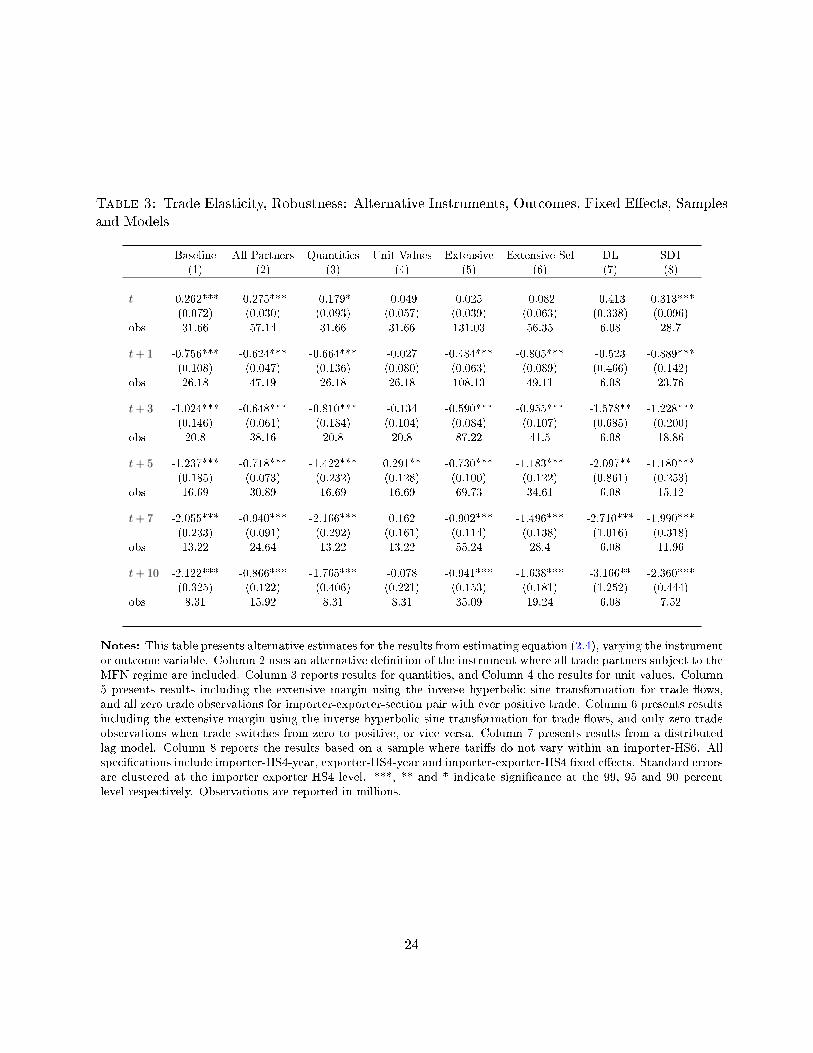
Table 3: Trade Elasticity, Robustness: Alternative Instruments, Outcomes, Fixed E�ects, Samplesand Models

Baseline All Partners Quantities Unit Values Extensive Extensive Sel DL SD1(1) (2) (3) (4) (5) (6) (7) (8)

t -0.262*** -0.275*** -0.179* -0.049 0.025 -0.082 -0.413 -0.313***(0.072) (0.030) (0.093) (0.057) (0.039) (0.063) (0.338) (0.096)

obs 31.66 57.14 31.66 31.66 131.03 56.35 6.08 28.7

t+ 1 -0.756*** -0.624*** -0.664*** -0.027 -0.484*** -0.805*** -0.523 -0.889***(0.108) (0.047) (0.136) (0.080) (0.063) (0.089) (0.466) (0.142)

obs 26.18 47.19 26.18 26.18 108.13 49.11 6.08 23.76

t+ 3 -1.024*** -0.648*** -0.810*** -0.134 -0.590*** -0.955*** -1.578** -1.228***(0.146) (0.061) (0.184) (0.104) (0.084) (0.107) (0.685) (0.200)

obs 20.8 38.16 20.8 20.8 87.22 41.5 6.08 18.86

t+ 5 -1.237*** -0.718*** -1.422*** 0.291** -0.730*** -1.183*** -2.097** -1.180***(0.185) (0.073) (0.232) (0.128) (0.100) (0.122) (0.861) (0.253)

obs 16.69 30.89 16.69 16.69 69.73 34.61 6.08 15.12

t+ 7 -2.055*** -0.940*** -2.166*** 0.162 -0.902*** -1.496*** -2.710*** -1.990***(0.233) (0.091) (0.292) (0.161) (0.114) (0.138) (1.016) (0.318)

obs 13.22 24.64 13.22 13.22 55.24 28.4 6.08 11.96

t+ 10 -2.122*** -0.866*** -1.765*** -0.078 -0.941*** -1.638*** -3.166** -2.360***(0.325) (0.122) (0.406) (0.221) (0.153) (0.181) (1.252) (0.444)

obs 8.31 15.92 8.31 8.31 35.09 19.24 6.08 7.52

Notes: This table presents alternative estimates for the results from estimating equation (2.4), varying the instrumentor outcome variable. Column 2 uses an alternative de�nition of the instrument where all trade partners subject to theMFN regime are included. Column 3 reports results for quantities, and Column 4 the results for unit values. Column5 presents results including the extensive margin using the inverse hyperbolic sine transformation for trade �ows,and all zero trade observations for importer-exporter-section pair with ever positive trade. Column 6 presents resultsincluding the extensive margin using the inverse hyperbolic sine transformation for trade �ows, and only zero tradeobservations when trade switches from zero to positive, or vice versa. Column 7 presents results from a distributedlag model. Column 8 reports the results based on a sample where tari�s do not vary within an importer-HS6. Allspeci�cations include importer-HS4-year, exporter-HS4-year and importer-exporter-HS4 �xed e�ects. Standard errorsare clustered at the importer-exporter-HS4 level. ***, ** and * indicate signi�cance at the 99, 95 and 90 percentlevel respectively. Observations are reported in millions.

24

A second instrument would be a change in the MFN bound, which is the maximum tari� a country

in the WTO can apply against other countries. While these are likely less discretionary, the MFN

bounds are set in the WTO accession treaty and very hard to change ex-post. The lack of instances

of changes in the bounds implies there is insu�cient variation in this instrument to estimate the

elasticity.

Measurement error A common concern with di�erenced speci�cations is that they can exacerbate

measurement error.21 While our baseline speci�cations are di�erenced, we note that the right-

hand-side variable is a change in tari�s, which are data that are extremely unlikely to su�er from

measurement error. This eliminates concerns that measurement error is biasing our estimates.

5 Applications and Relationship to Theory

We stress that equations (2.2), (2.3), and (2.4) are �model free,� and under our identi�cation as-

sumptions will produce estimates of εh by de�nition. The mapping between these estimates and

parameters in theoretical models then depends on model structure. This section has two parts. The

�rst maps our estimates to the long-run elasticity applicable in static trade models, and performs

welfare gains from trade calculations. The second develops a simple dynamic framework of sluggish

adjustment to trade cost shocks, and explores what the time path of our estimates implies for the

parameters governing adjustment.

5.1 The Long-Run Trade Elasticity and Welfare

This section presents a mapping from the estimated εh to the long-run (steady state) trade elasticity,

the key parameter in static international trade models. We clarify two points. First, the estimation

of εh takes into account the time series behavior of tari�s as well as trade �ows. If in the data

tari�s exhibit any autocorrelation behavior after the initial impulse, the estimated εh will re�ect the

dynamic behavior of both trade �ows and tari�s. Thus, the εh itself does not answer the question

of what happens following a one-time permanent change in trade costs. However, we can use the

components of εh to recover the steady-state elasticity that applies in static (long-run) models.

Second, how the long-run estimated elasticity relates to structural model parameters depends on

whether the trade data used in estimation include tari� payments.

21As di�erencing two white noise processes doubles the variance of the resultant process.

25

Dynamic and static gravity We suppress the product dimension in the exposition to economize

on notation. Let the trade �ows follow the gravity relationship:

Xi,j,t ∝∞∏k=0

φθki,j,t−k · Si,t ·Dj,t (5.1)

where Si,t and Dj,t are the multilateral resistance terms, that vary by importer and exporter re-

spectively, but not country pair. The non-standard feature of (5.1) is that time-t trade �ows are

allowed to depend on past values of iceberg trade costs φi,j,t−k with a horizon-dependent elasticity

θk. This would be the case if, for example, adjustment of trade is sluggish, and conditions in the

past a�ect the trading relationships that exist in the present. Of course, this speci�cation nests the

traditional contemporaneous gravity equation, which obtains when θk = 0 ∀k > 0. The assumption

of dependence of current trade on past trade costs is falsi�able, and our empirical work can be viewed

as an econometric test of this assumption.

One can view the static gravity relationship as a steady-state version of (5.1). Suppose that all the

φi,j,t's and multilateral resistance terms are constant over time. In steady state:

Xi,j ∝ φ∑∞k=0 θk

i,j · Si ·Dj , (5.2)

which is the textbook gravity relationship. Equation (5.2) shows that the object of interest for static

international trade models is the long-run trade elasticity θ ≡∑∞

k=0 θk. We assume that the structure

of θk's is such that the long-run trade elasticity is �nite. This would be the case, for instance, if

θk = 0 ∀k > K <∞.

Mapping back to empirical estimates Plugging in the form of iceberg trade costs into (5.1)

and taking logs:

lnXi,j,t ∝∞∑k=0

(θk lnκi,j,t−k + θkτi,j,t−k) + lnSi,t + lnDj,t.

The impact of a single-period change in tari�s at t on trade at t+ k is:

∂ lnXi,j,t+k

∂τi,j,t≈ θk.

However, in the data tari� changes are persistent. The impact of a one-time permanent change in

tari�s that occurs between t− 1 and t on trade at t+ h is

∂ lnXi,j,t+h

∂τi,j,t=

h∑k=0

θk ≡ θh. (5.3)

26

Note the switch from a subscript on θk to a superscript on θh, to denote the cumulative nature of

the latter. As h → ∞, θh → θ, the long-run trade elasticity. As a practical matter, we can only

estimate parameters up to the horizon h = 10 years, and will by necessity treat the 10-year estimates

as re�ecting the long run. The time series behavior of point estimates suggests that this may be a

fair approximation.

We now turn to the question of how to recover θh from our estimates. The h-year di�erence in trade

�ows is:

∆h lnXi,j,t ≈∞∑k=0

θk∆hτi,j,t−k + ∆h lnSi,t + ∆h lnDj,t + ui,j,t, (5.4)

where the error term corresponds to the change in non-tari� bilateral trade costs, ui,j,t =∑∞

k=0 ∆hθk lnκi,j,t−k.

If there was a permanent shock ∆0τi,j,t to tari�s at a speci�c calendar t, then the h-period change

is simply equal to the initial change: ∆hτi,j,t = ∆0τi,j,t. In that case it is easy to verify from the

de�nition (2.1) that εh = θh, and it could just be estimated by regressing ∆h lnXi,j,t on that tari�

change for each h, which corresponds exactly to equation (2.2).

However, the tari� changes may be autocorrelated, and so a time-t innovation ∆0τi,j,t may be followed

by further changes later. Equation (2.3) �exibly captures the autocorrelation in tari�s by relating the

h-period change back to the initial impulse. Indeed, Figure 3 reports the estimates of this equation

and shows a moderate degree of mean-reversion in tari�s. Combining (2.3) and (5.4), the h-period

change in trade �ows has the following relationship to a time-t impulse in tari�s (dropping κ's, S's

and D's):

∆h lnXi,j,t ∝(θ0β

hτ + θ1β

h−1τ + θ2β

h−2τ + θ3β

h−3τ + ...+ θh

)∆0τi,j,t.

Intuitively, the h-period-ahead response of trade �ows to a one-unit initial change in tari�s is a

combination of the elasticities of trade changes to lagged trade costs θk and the best predictions of

what tari�s themselves will be k periods ahead following a time-t innovation in tari�s, βkτ . Combining

this relationship with (2.2), we can recover the elasticities to permanent trade cost changes θh from

our estimates of trade elasticities εh and the time series behavior of tari�s themselves βhτ :

εh = θh + θ1βh−1τ − βhτ

βhτ+ θ2

βh−2τ − βhτβhτ

+ θ3βh−3τ − βhτ

βhτ+ ...+ θh

1− βhτβhτ

. (5.5)

Thus, the elasticity to the permanent shock θh is a transformation of the εh and the βhτ estimates

reported above. Since this expression holds also for h = 0, (5.5) can be used to recover each θh

recursively. Once we have done that, we will treat the 10-year horizon θ10 as an estimate of the

long-run elasticity θ.

27

Trade �ows net and gross of tari�s The second important aspect of the interpretation of our

coe�cient estimates is whether the elasticity is de�ned with respect to spending inclusive or exclusive

of tari�s. Most theoretical gravity relationships relate spending by domestic agents to trade costs,

with the trade elasticity de�ned correspondingly. On the other hand, the data on our outcome

variable Xi,j,t does not include tari� payments.

To see the consequences of this disparity, denote by X̃i,j the steady state spending by consumers in

economy i on goods from j, and by θ̃ the elasticity of this consumer spending to trade costs:

X̃i,j ∝ φθ̃i,j · Si ·Dj . (5.6)

The elasticity θ̃ is relevant for the welfare gains from trade calculations, for example. Since X̃i,j =

(1 + τi,j)Xi,j and φi,j = κi,j · (1 + τi,j), we can rewrite (5.6) in terms of trade �ows exclusive of tari�

payments Xi,j , which are reported in our data:22

Xi,j ∝ κθ̃i,j (1 + τi,j)θ̃−1 · Si ·Dj . (5.7)

Comparing (5.7) to (5.2), the two elasticities have the following relationship: θ̃ = θ + 1. As an

example, in an Armington setting θ̃ corresponds to 1 − σ, where σ is the elasticity of substitution

between goods coming from di�erent origins. In that case, θ = −σ. In an Eaton-Kortum setting, θ̃

is the Frechet dispersion parameter. In that case, it can be recovered by adding 1 to our θ estimates.

Welfare gains from trade As is well known from Arkolakis, Costinot, and Rodríguez-Clare

(2012), the gains from trade relative to autarky in many quantitative trade models can be expressed

as a function of the trade elasticity and the domestic absorption share: 1− λ1/θ̃jj , with λjj the share

of spending on domestically-produced goods in total spending. As detailed above, we can obtain θ̃

from our estimates by �rst computing θh from the εh and βhτ 's as in (5.5). This calculation gives us

θ10 = −1.589. Treating this as our best estimate of the long-run tari�-exclusive trade elasticity θ,

we conclude that the welfare-relevant elasticity θ̃ is −0.942.

Figure 6 displays the gains from trade as a function of λjj , under our value of θ̃ and under an

elasticity of −5 considered by Arkolakis, Costinot, and Rodríguez-Clare (2012). As expected, the

gains from trade are substantially larger with our elasticity. For the US, gains from trade are 5.61%

for θ̃ = −0.942, compared to 1.0% for θ̃ = −5. The median welfare gain is 24.5% in the sample 64

countries, compared to 4.2% implied by θ̃ = −5.23 Table A11 reports the gains from trade under

22This calculation assumes that Xi,j is recorded as c.i.f. The relationship between θ̃ and θ is the same if Xi,j is f.o.b.,since the iceberg costs κi,j are log-additive and make up the error term in our estimation.

23We use data from the OECD IO tables for 64 countries for the year 2006, the midpoint of our trade and tari� sample.We compute import penetration by dividing imports by gross output as in Arkolakis, Costinot, and Rodríguez-Clare(2012).

28

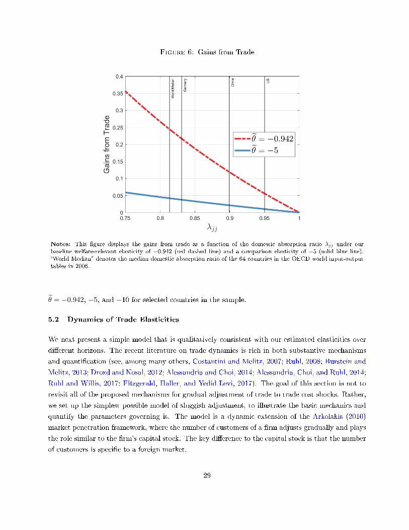
Figure 6: Gains from Trade

Notes: This �gure displays the gains from trade as a function of the domestic absorption ratio λjj under ourbaseline welfare-relevant elasticity of −0.942 (red dashed line) and a comparison elasticity of −5 (solid blue line).�World Median� denotes the median domestic absorption ratio of the 64 countries in the OECD world input-outputtables in 2006.

θ̃ = −0.942, −5, and −10 for selected countries in the sample.

5.2 Dynamics of Trade Elasticities

We next present a simple model that is qualitatively consistent with our estimated elasticities over

di�erent horizons. The recent literature on trade dynamics is rich in both substantive mechanisms

and quanti�cation (see, among many others, Costantini and Melitz, 2007; Ruhl, 2008; Burstein and

Melitz, 2013; Drozd and Nosal, 2012; Alessandria and Choi, 2014; Alessandria, Choi, and Ruhl, 2014;

Ruhl and Willis, 2017; Fitzgerald, Haller, and Yedid-Levi, 2017). The goal of this section is not to

revisit all of the proposed mechanisms for gradual adjustment of trade to trade cost shocks. Rather,

we set up the simplest possible model of sluggish adjustment, to illustrate the basic mechanics and

quantify the parameters governing it. The model is a dynamic extension of the Arkolakis (2010)

market penetration framework, where the number of customers of a �rm adjusts gradually and plays

the role similar to the �rm's capital stock. The key di�erence to the capital stock is that the number

of customers is speci�c to a foreign market.

29

Firm's problem Consider a representative �rm with a constant marginal cost c, selling its good

domestically and abroad. The �rm's problem is separable by market, and thus without loss of

generality we only model exports to a single foreign country. Since there is only one source and one

destination, we drop the i, j subscripts to economize on notation. As in Burstein, Neves, and Rebelo

(2003) and others, sales in a foreign country require local distribution services, that are combined in

�xed proportions with the exported good.

The foreign consumer pays the price

pct = pxt (1 + τt) + d,

where pxt denotes the exporter's fob price, τt the ad-valorem tari�, and d the per unit cost of local

distribution services.

The �rm commands monopoly power, and foreign demand exhibits a constant elasticity σ. Normal-

izing the aggregate foreign demand shifters to unity, the �rm faces the demand curve

qt = nt (pct)−σ ,

where nt is the mass of foreign consumers the �rm reaches. The �rm's optimal price is

pxt =σ

σ − 1c+

1

σ − 1

d

1 + τt. (5.8)

The price received by the producer is decreasing in tari�s, because higher tari�s increase the costs

of foregone sales at the margin. This feature of the model is consistent with the unit value response

documented in Table 3, and implies that the tari� passthrough to the consumer is incomplete.

The exporter price is also greater than the price in the absence of distribution costs, because the

monopolist does not internalize foregone sales by the distribution sector. The �rm's �ow pro�ts from

exporting are ntπ (τt), where π(.) is a decreasing function in tari�s.

As in Arkolakis (2010), the �rm incurs costs to reach foreign consumers. The mass of foreign

consumers available for the �rm to sell to evolves according to the accumulation equation

nt+1 = nt (1− δ) + at, (5.9)

where at is the mass of newly added customers in the foreign country. We assume that adding a

new customers requires a payment of f (a), where f ′ > 0 and f ′′ > 0, and that the existing mass of

consumers already reached by the �rm depreciates at rate δ.

The �rm discounts at interest rate r, correctly predicts the future path of tari�s, and maximizes the

30

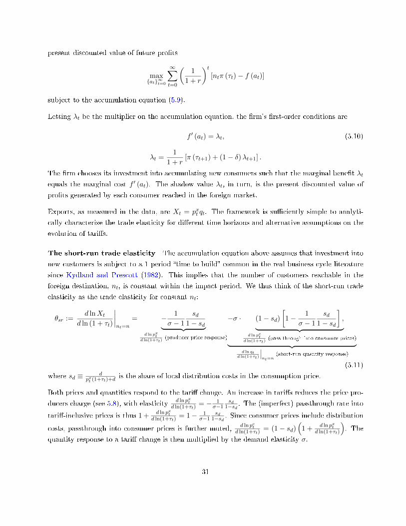
present discounted value of future pro�ts

max{at}∞t=0

∞∑t=0

(1

1 + r

)t[ntπ (τt)− f (at)]

subject to the accumulation equation (5.9).

Letting λt be the multiplier on the accumulation equation, the �rm's �rst-order conditions are

f ′ (at) = λt, (5.10)

λt =1

1 + r[π (τt+1) + (1− δ)λt+1] .

The �rm chooses its investment into accumulating new consumers such that the marginal bene�t λtequals the marginal cost f ′ (at). The shadow value λt, in turn, is the present discounted value of

pro�ts generated by each consumer reached in the foreign market.

Exports, as measured in the data, are Xt = pxt qt. The framework is su�ciently simple to analyti-

cally characterize the trade elasticity for di�erent time horizons and alternative assumptions on the

evolution of tari�s.

The short-run trade elasticity The accumulation equation above assumes that investment into

new customers is subject to a 1-period �time-to-build� common in the real business cycle literature

since Kydland and Prescott (1982). This implies that the number of customers reachable in the

foreign destination, nt, is constant within the impact period. We thus think of the short-run trade

elasticity as the trade elasticity for constant nt:

θsr :=d lnXt

d ln (1 + τt)

∣∣∣∣nt=n

= − 1

σ − 1

sd1− sd︸ ︷︷ ︸

d ln pxtd ln(1+τt)

(producer price response)

−σ · (1− sd)[1− 1

σ − 1

sd1− sd

],︸ ︷︷ ︸

d ln pctd ln(1+τt)

(pass-through into consumer prices)︸ ︷︷ ︸d ln qt

d ln(1+τt)

∣∣∣nt=n

(short-run quantity response)

(5.11)

where sd ≡ dpxt (1+τt)+d

is the share of local distribution costs in the consumption price.

Both prices and quantities respond to the tari� change. An increase in tari�s reduces the price pro-

ducers charge (see 5.8), with elasticity d ln pxtd ln(1+τt)

= − 1σ−1

sd1−sd . The (imperfect) passthrough rate into

tari�-inclusive prices is thus 1 +d ln pxt

d ln(1+τt)= 1− 1

σ−1sd

1−sd . Since consumer prices include distribution

costs, passthrough into consumer prices is further muted, d ln pctd ln(1+τt)

= (1− sd)(

1 +d ln pxt

d ln(1+τt)

). The

quantity response to a tari� change is then multiplied by the demand elasticity σ.

31

The long-run trade elasticity In addition to the short-run changes discussed above, the �rm's

customer base nt adjusts in the long run. We think of the long-run trade elasticity as the response of

trade in steady state to a change in steady state tari�s. Dropping time subscripts to denote steady

state values, the long-run elasticity is:

θlr :=d lnX

d ln (1 + τ)= θsr + −σ (1− sd)

(f ′′ (a) a

f ′ (a)

)−1︸ ︷︷ ︸d lnn

d ln(1+τ)(response of customer base)

, (5.12)

and thus adds the customer base response to the short-run elasticity. The customer base responds

to the tari� change with the same elasticity as investment into new consumers ( d lnnd ln(1+τ) = d ln a

d ln(1+τ)).

Investment into new consumers, in turn, is determined by the curvature of market penetration costs

f(a), and the shadow value λ (see equation 5.10). Since the shadow value is determined by the e�ect of

tari�s on per-customer �ow pro�ts π, we have d ln ad ln(1+τ) =

(f ′′(a)af ′(a)

)−1d lnλ

d ln(1+τ) =(f ′′(a)af ′(a)

)−1d lnπ

d ln(1+τ) .

The elasticity of per-customer �ow pro�ts to tari�s is d lnπd ln(1+τ) = −σ (1− sd). Putting these pieces

together delivers (5.12).

Transitional dynamics Consider a tari� change at time t0 and its e�ect on exports at time t0+h.

Before t0, the dynamic system is assumed to be in steady state. For the dynamic response of trade

�ows to tari�s, both the history of tari�s between t0 and t0+h and expectations about tari�s beyond

horizon t0+h matter. More precisely, for an arbitrary sequence of tari� changes relative to the steady

state d ln (1 + τt0), d ln (1 + τt0+1), d ln (1 + τt0+2) , ..., the e�ect on exports at time t0 + h is

d lnXt0+h = −σ (δ + r) (1− sd)1 + r

δ

(f ′′ (a) a

f ′ (a)

)−1 h−1∑`=0

(1− δ)h−(`+1)∞∑k=0

(1− δ1 + r

)kd ln (1 + τt0+`+k+1)

+θsrd ln (1 + τt0+h) .

Since this expression is complicated, we next consider two simpler examples, both reasonably good

descriptions of the observed tari� changes in our data.

Example 1: tari� constant after 1 period First, consider a surprise change in the tari�

sequence of the form d ln (1 + τt0), d ln (1 + τt0+1) = d ln (1 + τ>t0), d ln (1 + τt0+2) = d ln (1 + τ>t0),

d ln (1 + τt0+3) = d ln (1 + τ>t0),..., all expressed relative to the initial steady state. That is, the tari�

change takes one particular value, d ln (1 + τt0), in the impact period, and is subsequently constant

at d ln (1 + τ>t0). Note that this example nests a one-o� permanent change in tari�s (τt0 = τ>t0),

and is a good approximation of our estimated impulse response function in Figure 3.

32

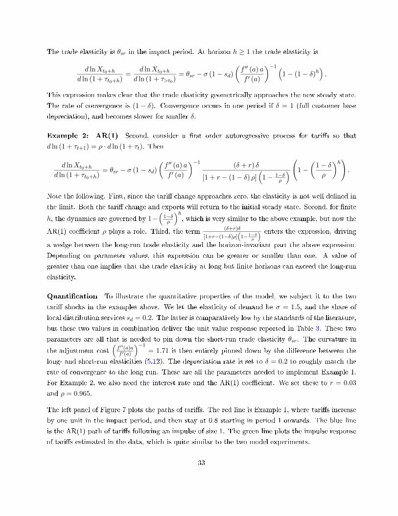
The trade elasticity is θsr in the impact period. At horizon h ≥ 1 the trade elasticity is

d lnXt0+h

d ln (1 + τt0+h)=

d lnXt0+h

d ln (1 + τ>t0)= θsr − σ (1− sd)

(f ′′ (a) a

f ′ (a)

)−1 (1− (1− δ)h

).

This expression makes clear that the trade elasticity geometrically approaches the new steady state.

The rate of convergence is (1− δ). Convergence occurs in one period if δ = 1 (full customer base

depreciation), and becomes slower for smaller δ.

Example 2: AR(1) Second, consider a �rst order autoregressive process for tari�s so that

d ln (1 + τt+1) = ρ · d ln (1 + τt). Then

d lnXt0+h

d ln (1 + τt0+h)= θsr − σ (1− sd)

(f ′′ (a) a

f ′ (a)

)−1 (δ + r) δ

[1 + r − (1− δ) ρ](

1− 1−δρ

) (1−(

1− δρ

)h).

Note the following. First, since the tari� change approaches zero, the elasticity is not well de�ned in

the limit. Both the tari� change and exports will return to the initial steady state. Second, for �nite

h, the dynamics are governed by 1−(1−δρ

)h, which is very similar to the above example, but now the

AR(1) coe�cient ρ plays a role. Third, the term (δ+r)δ

[1+r−(1−δ)ρ](1− 1−δ

ρ

) enters the expression, driving

a wedge between the long-run trade elasticity and the horizon-invariant part the above expression.

Depending on parameter values, this expression can be greater or smaller than one. A value of

greater than one implies that the trade elasticity at long but �nite horizons can exceed the long-run

elasticity.

Quanti�cation To illustrate the quantitative properties of the model, we subject it to the two

tari� shocks in the examples above. We let the elasticity of demand be σ = 1.5, and the share of

local distribution services sd = 0.2. The latter is comparatively low by the standards of the literature,

but these two values in combination deliver the unit value response reported in Table 3. These two

parameters are all that is needed to pin down the short-run trade elasticity θsr. The curvature in

the adjustment cost(f ′′(a)af ′(a)

)−1= 1.71 is then entirely pinned down by the di�erence between the

long- and short-run elasticities (5.12). The depreciation rate is set to δ = 0.2 to roughly match the

rate of convergence to the long run. These are all the parameters needed to implement Example 1.

For Example 2, we also need the interest rate and the AR(1) coe�cient. We set these to r = 0.03

and ρ = 0.965.

The left panel of Figure 7 plots the paths of tari�s. The red line is Example 1, where tari�s increase

by one unit in the impact period, and then stay at 0.8 starting in period 1 onwards. The blue line

is the AR(1) path of tari�s following an impulse of size 1. The green line plots the impulse response

of tari�s estimated in the data, which is quite similar to the two model experiments.

33

Figure 7: Time Path of Elasticities in the Dynamic Model

Notes: This �gure illustrates the trade elasticities as implied by the model.

The right panel of Figure 7 depicts the trade elasticities. The green line is the econometric estimates.

Because the data are annual, and it is unlikely that all tari� changes went into e�ect on January 1,

the year-zero trade elasticity is most likely subject to partial-year e�ects. Thus, for the purposes of

comparing to the model, we consider the h = 1 empirical estimate to be the impact elasticity θsr.

The red and blue lines depict the model trade elasticity in the two experiments. They are nearly

indistinguishable from each other.

The model succeeds in delivering a smooth path of adjustment that lasts a decade. The key parameter

for the speed of adjustment is the depreciation rate δ. The slow adjustment observed in the data

implies that δ is substantially below 1. The main shortcoming of the model is its overshooting of

the short-run elasticity, which in the data is about 0.7. The model short-run elasticity is governed

by only two parameters, σ and sd (see 5.11). The former has to be above 1 to be consistent with

monopolistic competition; the latter has to lie between 0 and 1. It turns out that there exists no

combination of σ and sd satisfying these restrictions that delivers θsr < 1.

6 Conclusion

We develop a novel method to estimate the trade elasticity, a key parameter in virtually all models in

international economics. To tackle the endogeneity problem that tari�s might be lower in products

34

where countries expect the largest trade �ows, we develop an instrument that relies on the WTO's

MFN principle. We estimate trade elasticities at di�erent horizons, and �nd short-run values of about

−0.7, and long-run values close to −1.75. Our estimates are robust to alternative speci�cations of

the instrument and controls, and uniformly larger than OLS. Our estimates are also not speci�c to a

particular model framework, and apply to all models that have a gravity speci�cation for trade �ows

in the long run.

Our long-run estimates imply the welfare-relevant trade elasticity is around 1 in absolute value. This

is signi�cantly smaller than conventional wisdom in the literature, suggesting the welfare gains from

trade are larger than previously thought. Our �nding that the trade elasticity di�ers by horizon

and only converges to the �long-run� after about 7-10 years implies substantial adjustment costs to

changing trade volumes.

35

References

Alessandria, George and Horag Choi. 2014. �Establishment heterogeneity, exporter dynamics, and

the e�ects of trade liberalization.� Journal of International Economics 94 (2):207 � 223.

Alessandria, George, Horag Choi, and Kim Ruhl. 2014. �Trade Adjustment Dynamics and the Welfare

Gains from Trade.� NBER Working Papers 20663, National Bureau of Economic Research, Inc.

Anderson, James and Eric van Wincoop. 2004. �Trade Costs.� Journal of Economic Literature

42 (3):691�751.

Anderson, James E. 1979. �A Theoretical Foundation for the Gravity Equation.� American Economic

Review 69 (1):106�116.

Anderson, James E. and Eric van Wincoop. 2003. �Gravity with Gravitas: A Solution to the Border

Puzzle.� American Economic Review 93 (1):170�192.

Arkolakis, Costas. 2010. �Market Penetration Costs and the New Consumers Margin in International

Trade.� Journal of Political Economy 118 (6):1151�1199.

Arkolakis, Costas, Arnaud Costinot, and Andrés Rodríguez-Clare. 2012. �New Trade Models, Same

Old Gains?� American Economic Review 102 (1):94�130.

Bagwell, Kyle and Robert W. Staiger, editors. 2016. Handbook of Commercial Policy, vol. 1. Elsevier-

North Holland.

Baldwin, Richard and Daria Taglioni. 2006. �Gravity for Dummies and Dummies for Gravity Equa-

tions.� NBER Working Paper 12516.

Bas, Maria, Thierry Mayer, and Mathias Thoenig. 2017. �From micro to macro: Demand, supply,

and heterogeneity in the trade elasticity.� Journal of International Economics 108:1 � 19.

Bellemare, Marc F. and Casey J. Wichman. 2020. �Elasticities and the Inverse Hyperbolic Sine

Transformation.� Oxford Bulletin of Economics and Statistics 82 (1):50�61.

Bown, Chad P. and Meredith A Crowley. 2013. �Import Protection, Business Cycles, and Exchange

Rates: Evidence from the Great Recession.� Journal of International Economics 90 (1):50�64.

���. 2016. �The Empirical Landscape of Trade Policy.� In The Handbook of Commercial Policy,

vol. 1, edited by Kyle Bagwell and Robert W. Staiger, chap. 1. Elsevier-North Holland, 3�108.

Broda, Christian and David Weinstein. 2006. �Globalization and the Gains from Variety.� Quarterly

Journal of Economics 121 (2):541�85.

36

Burbidge, John B., Lonnie Magee, and A. Leslie Robb. 1988. �Alternative Transformations to Handle

Extreme Values of the Dependent Variable.� Journal of the American Statistical Association

83 (401):123�127.

Burstein, Ariel and Marc Melitz. 2013. �Trade Liberalization and Firm Dynamics.� In Advances in

Economics and Econometrics Tenth World Congress. Applied Economics, vol. 2. Cambridge, UK:

Cambridge University Press.

Burstein, Ariel T., Joao C. Neves, and Sergio Rebelo. 2003. �Distribution costs and real exchange rate

dynamics during exchange-rate-based stabilizations.� Journal of Monetary Economics 50 (6):1189�

1214.

Caliendo, Lorenzo and Fernando Parro. 2015. �Estimates of the Trade and Welfare E�ects of

NAFTA.� Review of Economic Studies 82 (1):1�44.

Canova, Fabio and Luca Sala. 2009. �Back to square one: Identi�cation issues in DSGE models.�

Journal of Monetary Economics 56 (4):431 � 449.

Costantini, James and Marc Melitz. 2007. �The Dynamics of Firm-Level Adjustment to Trade

Liberalization.� In The Organization of Firms in a Global Economy, edited by E. Helpman,

D. Marin, and T. Verdier. Cambridge, MA: Harvard University Press.

Drozd, Lukasz A. and Jaromir B. Nosal. 2012. �Understanding International Prices: Customers as

Capital.� American Economic Review 102 (1):364�95.

Eaton, Jonathan and Samuel S. Kortum. 2002. �Technology, Geography, and Trade.� Econometrica

70 (5):1741�1779.

Fajgelbaum, Pablo D., Pinelopi K. Goldberg, Patrick J. Kennedy, and Amit K. Khandelwal. 2020.

�The Return to Protectionism.� Quarterly Journal of Economics 135 (1):1�55.

Feenstra, Robert. 1994. �New Product Varieties and the Measurement of International Prices.�

American Economic Review 84 (1):157�77.

Feenstra, Robert C., Philip Luck, Maurice Obstfeld, and Katheryn N. Russ. 2018. �In Search of the

Armington Elasticity.� Review of Economics and Statistics 100 (1):135�150.

Fitzgerald, Doireann and Stefanie Haller. 2018. �Exporters and shocks.� Journal of International

Economics 113 (C):154�171.

Fitzgerald, Doireann, Stefanie Haller, and Yaniv Yedid-Levi. 2017. �How Exporters Grow.� Working

papers, School of Economics, University College Dublin.

37

Fontagné, Lionel, Philippe Martin, and Gianluca Ore�ce. 2018. �The international elasticity puzzle

is worse than you think.� Journal of International Economics 115:115 � 129.

Giri, Rahul, Kei-Mu Yi, and Hakan Yilmazkuday. 2020. �Gains from Trade: Does Sectoral Hetero-

geneity Matter?� NBER Working Paper 26741.

Gourio, François and Leena Rudanko. 2014. �Customer Capital.� Review of Economic Studies

81 (2):1102�1136.

Head, Keith and Thierry Mayer. 2015. �Gravity Equations: Workhorse, Toolkit, and Cookbook.� In

Handbook of International Economics, vol. 4, edited by Elhanan Helpman, Kenneth Rogo�, and

Gita Gopinath. Elsevier B.V., 131�195.

Head, Keith and John Ries. 2001. �Increasing Returns versus National Product Di�erentiation as an

Explanation for the Pattern of U.S.-Canada Trade.� American Economic Review 91 (4):858�876.

Jordà, Òscar. 2005. �Estimation and Inference of Impulse Responses by Local Projections.� American

Economic Review 95 (1):161�182.

Kydland, Finn E and Edward C Prescott. 1982. �Time to Build and Aggregate Fluctuations.�

Econometrica 50 (6):1345�1370.

Melitz, Marc J. 2003. �The Impact of Trade on Intra-Industry Reallocations and Aggregate Industry

Productivity.� Econometrica 71 (6):1695�1725.

Pierce, Justin R. and Peter K. Schott. 2016. �The Surprisingly Swift Decline of US Manufacturing

Employment.� American Economic Review 106 (7):1632�62.

Redding, Stephen and Anthony J. Venables. 2004. �Economic geography and international inequal-

ity.� Journal of International Economics 62 (1):53�82.

Romalis, John. 2007. �NAFTA's and CUSFTA's Impact on International Trade.� Review of Eco-

nomics and Statistics 89 (3):416�435.

Ruhl, Kim J. 2008. �The International Elasticity Puzzle.� Working Paper.

Ruhl, Kim J. and Jonathan L. Willis. 2017. �New Exporter Dynamics.� International Economic

Review 58 (3):703�726.

Sequeira, Sandra. 2016. �Corruption, Trade Costs, and Gains from Tari� Liberalization: Evidence

from Southern Africa.� American Economic Review 106 (10):3029�63.

Simonovska, Ina and Michael E. Waugh. 2014. �The Elasticity of Trade: Estimates and Evidence.�

Journal of International Economics 92 (1):34�50.

38

Sims, Christopher A. 1980. �Macroeconomics and Reality.� Econometrica 48 (1):1�48.

Soderbery, Anson. 2015. �Estimating import supply and demand elasticities: Analysis and implica-

tions.� Journal of International Economics 96 (1):1�17.

���. 2018. �Trade elasticities, heterogeneity, and optimal tari�s.� Journal of International Eco-

nomics 114:44 � 62.

World Trade Organization. 2014. �World Tari� Pro�les 2014.� Geneva: WTO, UNCTAD, and ITC.

39

Appendix A Additional Theory

This appendix provides an example of a model of exporting that delivers the trade elasticity estimat-ing equation. We stress that this is only one possible model that can deliver our estimating equation.We omit the product subcript to economize on notation. A �rm of measure 1 from country i sellingto country j has time t sales equal to:

xijt =p1−σijt

P 1−σjt

Xjt,

where Xjt is aggregate expenditure in j, Pjt is the price index, and pijt is the price charged bythe �rm. The �rm is monopolistically competitive, and thus its price is a constant markup overmarginal cost: pijt = σ

σ−1φijtc1−σit , where φijt is the iceberg trade cost at time t, and cit is the unit

cost of production. Then, its sales can be written as a product of bilateral, source, and destinationcomponents:

xijt = φ1−σijt S̃itD̃jt,

where S̃it ≡ c1−σit and D̃jt ≡(

σσ−1

)1−σXjt/P

1−σjt . Period variable pro�ts are a constant fraction of

sales:

πijt =1

σxijt.

There is a mass Mijt of �rms selling from i to j at time t. Then total trade �ows from i to j are:

Xijt = Mijtxijt

= Mijtφ1−σijt S̃itD̃jt.

Let a fraction δ of last year's �rms survive into this year, and let mijt be the new measure of �rmsappearing between t − 1 and t. This formulation nests extensive margin (where mijt is the mass ofnew �rm entrants as in Melitz, 2003), and customer base (where mijt is the mass of new customersadded by the �rm as in Arkolakis, 2010, and Section 5.2). The accounting equation for the mass of�rms is:

Mijt = Mijt−1(1− δ) +mijt.

Iterating backward:

Mijt =∞∑k=0

(1− δ)kmijt−k.

Suppose for simplicity that there are no per period �xed costs of exporting, so that all �rms whoever started exporting continue until experiencing the exogenous death shock. Each year a mass 1of �rms is born, or equivalently receives a potential opportunity to export to j. These �rms face a

40

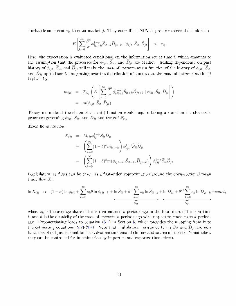
stochastic sunk cost εij to enter market j. They enter if the NPV of pro�ts exceeds the sunk cost:

E

[ ∞∑k=0

βk

σφ1−σijt+kS̃it+kD̃jt+k | φijt, S̃it, D̃jt

]> εij .

Here, the expectation is evaluated conditional on the information set at time t, which amounts tothe assumption that the processes for φijt, S̃it, and D̃jt are Markov. Adding dependence on pasthistory of φijt, S̃it, and D̃jt will make the mass of entrants at t a function of the history of φijt, S̃it,and D̃jt up to time t. Integrating over the distribution of sunk costs, the mass of entrants at time tis given by:

mijt = Fεij

(E

[ ∞∑k=0

βk

σφ1−σijt+kS̃it+kD̃jt+k | φijt, S̃it, D̃jt

])= m(φijt, S̃it, D̃jt)

To say more about the shape of the m(.) function would require taking a stand on the stochasticprocesses governing φijt, S̃it, and D̃jt and the cdf Fεij .

Trade �ows are now:

Xijt = Mijtφ1−σijt S̃itD̃jt

=

( ∞∑k=0

(1− δ)kmijt−k

)φ1−σijt S̃itD̃jt

=

( ∞∑k=0

(1− δ)km(φijt−k, S̃it−k, D̃jt−k)

)φ1−σijt S̃itD̃jt.

Log bilateral ij �ows can be taken as a �rst-order approximation around the cross-sectional meantrade �ow Xt:

lnXijt ≈ (1− σ) lnφijt +∞∑k=0

skθ lnφijt−k + ln S̃it + θS∞∑k=0

sk ln S̃it−k︸ ︷︷ ︸Sit

+ ln D̃jt + θD∞∑k=0

sk ln D̃jt−k︸ ︷︷ ︸Djt

+const,

where sk is the average share of �rms that entered k periods ago in the total mass of �rms at timet, and θ is the elasticity of the mass of entrants k periods ago with respect to trade costs k periodsago. Exponentiating leads to equation (5.1) in Section 5, which provides the mapping from it tothe estimating equations (2.2)-(2.4). Note that multilateral resistance terms Sit and Djt are nowfunctions of not just current but past destination demand shifters and source unit costs. Nonetheless,they can be controlled for in estimation by importer- and exporter-time e�ects.

41

Appendix B Data

Figure A1: Fraction of World Imports (Average, %)

05

10

15

USA

DEU

CHN

JPN

GBR

FRA

ITA

NLD

HKG

CAN

BEL

KOR

ESP

MEX

IND

SGP

CHE

AUS

RUS

POL

AUT

BRA

SW

E

TUR

MYS

THA

CZE

ARE

DNK

IDN

RoW

Notes: This �gure shows the average fraction of world trade �ows by importer in our sample.

42

Figure A2: Fraction of World Imports: MFN vs. non-MFN (%)

02

04

06

0

1990s 2000s 2010s

MFN Non−MFN

Notes: This �gure shows the average fraction of world trade that is subject to MFN tari�s and non-MFN tari�s bydecade in our sample.

43

Figure A3: Fraction of World Imports by HS Section (Average, %)

01

02

03

0

16 17 5 6 15 11 7 18 14 4 2 20 10 1 13 9 12 8 3 21 19

Notes: This �gure shows the average fraction of trade that is in each HS Section in our sample.

Table A1: HS Codes Mapping Across Revisions

Mapped to:HS-92 HS-96 HS-02 HS-07 HS-12

HS-96 89.38HS-02 81.55 90.81

Mapped from: HS-07 73.34 80.74 88.48HS-12 68.17 74.91 81.81 91.93HS-17 61.85 67.92 73.62 81.99 88.05

Notes: This table presents the fraction of HS codes that can be mapped uniquely from as HS revision in the �Mappedfrom� row to an HS revision in a �Mapped to� column. All numbers are in percentages.

44

Table A2: Instrument � Illustration

Importer MFN Trade Partners Major Trade Partners Major Trade Partners Treatment Control ExcludedAggregate HS 6403

2005 2006 2005 2006 2005 2006(1) (2) (3) (4) (5) (6) (7) (8) (9)

Panel A: Germany

USA USA FRA FRA ITA ITA HKG ITA CHNCHN CHN CHN CHN CHN CHN KOR VNM INDJPN JPN NLD NLD VNM VNM SGP PRT USAKOR KOR ITA ITA PRT PRT NZL AUT JPNIND IND USA USA AUT AUT CAN NLDCAN CAN GBR GBR IND IND AUS SVKHKG HKG BEL BEL NLD NLD PRK IDNSGP RUS AUT AUT SVK SVK ESPBRA SGP CHE CHE ESP IDN GBRRUS BRA JPN JPN ROU ROU FRA

Panel B: Japan

CHN CHN CHN CHN CHN CHN GBR KHM CHNUSA USA USA USA ITA ITA PRT MMR ITAKOR KOR AUS SAU KHM KHM BRA BGD VNMAUS AUS IDN ARE VNM VNM MAR MEX IDNITA ITA KOR AUS IDN IDN IND LAO ESPCAN FRA DEU IDN MMR MMR CHE NPL FRADEU CAN THA KOR BGD BGD HUN LBN DEUFRA DEU MYS QAT ESP ESP SVK THAVNM VNM ARE DEU FRA FRA LKA USADNK DNK SAU THA DEU DEU AUT KOR

Panel C: USACHN CHN CAN CAN CHN CHN PRT MEX CHNJPN JPN CHN CHN ITA ITA SVK CAN ITADEU DEU MEX MEX BRA BRA POL DOM BRAKOR KOR JPN JPN VNM VNM HKG ISR VNMITA ITA DEU DEU IDN IDN HUN MAR IDNGBR GBR KOR KOR THA THA CHE COL THAFRA FRA GBR VEN MEX MEX ALB SLV ESPIND IND FRA GBR ESP ESP BGR AUS INDHKG HKG ITA FRA IND IND DNK ZAF FRAVNM VNM MYS MYS DOM DOM AUT PER DEU

Notes: This table illustrates the construction of our instrument, using as an example product code 6403 �Footwear;with outer soles of rubber, plastics, leather or composition leather and uppers of leather� in 2006. Columns 1-2 listthe top exporters to three importing countries � USA, Germany and Japan � exporting under the MFN regime inperiods t = 2006 and t − 1 = 2005. Columns 3-4 list the importing countries' major aggregate trading partners inthese periods. Columns 5-6 list the major trading partners in product 6403. Columns 7-9 then list the main countriesin the treatment, control and excluded group for imports of product 6403 to the three importing countries.

45

TableA3:HSSections

Code

Nam

e

7PLAST

ICSANDARTICLESTHEREOF;RUBBERANDARTICLESTHEREOF

8RAW

HID

ESANDSK

INS,

LEATHER,FURSK

INSANDARTICLESTHEREOF;

SADDLERYANDHARNESS;TRAVELGOODS,

9WOODANDARTICLESOFWOOD;WOODCHARCOAL;

CORKANDARTICLESOFCORK;MANUFA

CTURESOFST

RAW,

OFESP

ARTOOROFOTHERPLAITINGMATERIALS;

BASK

ETWAREANDWICKERWORK

10PULPOFWOODOROFOTHERFIBROUSCELLULOSICMATERIAL;

RECOVERED(W

ASTEANDSC

RAP)PAPERORPAPERBOARD;

PAPERANDPAPERBOARDANDARTICLESTHEREOF

11TEXTILESANDTEXTILEARTICLES

13ARTICLESOFST

ONE,PLAST

ER,CEMENT,ASB

EST

OS,

MICAORSIMILARMATERIALS;

15BASE

METALSANDARTICLESOFBASE

METAL

CERAMIC

PRODUCTS;

GLASS

ANDGLASSWARE

16MACHINERYANDMECHANICALAPPLIANCES;

ELECTRICALEQUIPMENT;PARTSTHEREOF;SO

UNDRECORDERSANDREPRODUCERS,

TELEVISIO

NIM

AGEANDSO

UNDRECORDERSAND

REPRODUCERS,

ANDPARTSANDACCESSORIESOFSU

CHARTICLES

ARTIFICIALFLOWERS;

ARTICLESOFHUMANHAIR

18OPTICAL,PHOTOGRAPHIC,CINEMATOGRAPHIC,MEASU

RING,

CHECKING,PRECISIO

N,MEDICALORSU

RGICALINST

RUMENTSANDAPPARATUS;

CLOCKSANDWATCHES;

MUSICALINST

RUMENTS;

PARTSANDACCESSORIESTHEREOF

20MISCELLANEOUSMANUFA

CTUREDARTICLES

Aggregated

1LIVEANIM

ALS;

ANIM

ALPRODUCTS

2VEGETABLEPRODUCTS

3ANIM

ALORVEGETABLEFA

TSANDOILSANDTHEIR

CLEAVAGEPRODUCTS

HANDBAGSANDSIMILARCONTAINERS;

ARTICLESOFANIM

ALGUT(O

THERTHANSILK-W

ORM

GUT)

4PREPAREDEDIBLEFA

TS;ANIM

ALORVEGETABLEWAXES

PREPAREDFOODST

UFFS;

BEVERAGES,

SPIRITSANDVINEGAR;TOBACCOANDMANUFA

CTUREDTOBACCOSU

BST

ITUTES

5MINERALPRODUCTS

6PRODUCTSOFTHECHEMICALORALLIEDINDUST

RIES

12FOOTWEAR,HEADGEAR,UMBRELLAS,

SUNUMBRELLAS,

WALKING-STICKS,

SEAT-STICKS,

WHIPS,

RID

ING-CROPSANDPARTSTHEREOF;

PREPAREDFEATHERSANDARTICLESMADETHEREWITH;

14NATURALORCULT

UREDPEARLS,

PRECIO

USORSE

MI-PRECIO

US

STONES,

PRECIO

USMETALS,

METALSCLADWITHPRECIO

USMETAL

ANDARTICLESTHEREOF;IM

ITATIO

NJE

WELLERY;COIN

17VEHICLES,

AIRCRAFT,VESSELSANDASSOCIATEDTRANSP

ORTEQUIPMENT

19ARMSANDAMMUNITIO

N;PARTSANDACCESSORIESTHEREOF

21WORKSOFART,COLLECTORS'

PIECESANDANTIQ

UES

Notes:Thistabledescribes

the21internationallycompatibleHS�Sections�,whichare

groupingsofHSproduct

codes.Wealsolist

the9HS

Sectionsthatweaggregate

inthemain

textinto

aSection`aggregate',asthereisinsu�cientvariationin

either

tari�sortrade�ow

sorboth

inthesesectionsto

estimate

theelasticity.

A5summarizestheestimatesforallsectionswithoutaggregation.

46

Appendix C Robustness

47

Table A4: Robustness: Local Projections

Panel A: Tari�s Panel B: TradeBaseline Zero Lag Five Lags Baseline Zero Lag Five Lags

(1) (2) (3) (4) (5) (6)t− 6 -0.099*** -0.090*** -0.102*** 0.097 0.028 0.305*

(0.006) (0.005) (0.007) (0.130) (0.110) (0.165)t− 5 -0.021*** -0.031*** . 0.217 0.275*** .

(0.005) (0.004) . (0.121) (0.105) .t− 4 -0.038*** -0.020*** . 0.004 -0.055 .

(0.005) (0.004) . (0.111) (0.093) .t− 3 -0.053*** -0.088*** . 0.075 -0.018 .

(0.005) (0.004) . (0.102) (0.087) .t− 2 -0.133*** -0.034*** . 0.242*** 0.128 .

(0.004) (0.004) . (0.089) (0.089) .t− 1 . -0.309*** . . 0.149** .

. (0.004 . . (0.072) .t . . . -0.262*** -0.147*** 0.166

. . . (0.072) (0.054) (0.138)t+ 1 0.890*** 0.851*** 0.842*** -0.673*** -0.535*** -0.109

(0.004) (0.003) (0.006) (0.096) (0.069) (0.175)t+ 2 0.846*** 0.830*** 0.788*** -0.716*** -0.588*** -0.129

(0.005) (0.003) (0.007) (0.109) (0.079) (0.206)t+ 3 0.831*** 0.818*** 0.769*** -0.851*** -0.758*** -0.481**

(0.005) (0.004) (0.008) (0.122) (0.086) (0.242)t+ 4 0.821*** 0.813*** 0.747*** -0.835*** -0.747*** -0.214

(0.006) (0.004) (0.009) (0.132) (0.094) (0.271)t+ 5 0.807*** 0.823*** 0.718*** -0.998*** -0.915*** -0.823***

(0.005) (0.004) (0.010) (0.149) (0.102) (0.308)t+ 6 0.776*** 0.786*** 0.663*** -1.006*** -0.875*** -0.496**

(0.006) (0.004) (0.011) (0.152) (0.101) (0.320)t+ 7 0.694*** 0.754*** 0.594*** -1.425*** -1.146*** -1.383***

(0.006) (0.004) (0.011) (0.162) (0.110) (0.352)t+ 8 0.668*** 0.716*** 0.552*** -1.269*** -1.145*** -0.932**

(0.007) (0.005) (0.012) (0.169) (0.117) (0.391)t+ 9 0.699*** 0.733*** 0.634*** -1.351*** -0.990*** -1.366***

(0.007) (0.005) (0.015) (0.198) (0.120) (0.513)t+ 10 0.715*** 0.720*** 0.641*** -1.517*** -1.054*** -1.635**

(0.008) (0.005) (0.018) (0.232) (0.139) (0.649)

Notes: This table presents the results from estimating the local projections equations (2.3) (Panel A) and (2.2) (PanelB). The �rst column in each panel presents the baseline local projects results, while the second and third columns ineach panel present results with 2 and 5 lags of tari�s and trade as pre-trend controls respectively. Standard errorsclustered by country-pair-product are in parentheses. ***, ** and * denote signi�cance at the 99, 95 and 90% levels.

48

Table A5: Trade Elasticity: Sectoral Heterogeneity

Mean Median 25 percentile 75 percentile(1) (2) (3) (4)

t -0.396 -0.407 -0.670 -0.117t+ 1 -0.851 -0.710 -1.116 -0.563t+ 2 -1.041 -0.798 -1.601 -0.465t+ 3 -1.381 -1.220 -2.044 -0.791t+ 4 -1.171 -1.100 -1.619 -0.710t+ 5 -1.683 -1.698 -2.060 -1.062t+ 6 -1.747 -1.651 -2.478 -0.887t+ 7 -3.082 -1.959 -3.731 -1.469t+ 8 -3.518 -2.324 -4.164 -1.218t+ 9 -3.352 -2.195 -3.248 -1.522t+ 10 -2.804 -2.794 -3.448 -1.906

Notes: This table presents results from estimating equation (2.4) at the HS Section-level for every horizon. Weinclude estimates for 11 HS Sections here, including one aggregated super-section as described in the text. Allspeci�cations include importer-HS4-year, exporter-HS4-year and importer-exporter-HS4 �xed e�ects.

49

Table A6: Elasticity Estimates, �Traditional Gravity,� Levels

(1) (2) (3) (4) (5) (6)

Panel A: Log-levels, OLSτi,j,p,t -3.696*** -4.468*** -6.696*** -2.734*** -1.040*** -0.892***

(0.020) (0.019) (0.046) (0.014) (0.022) (0.020)

R2 0.013 0.341 0.383 0.530 0.571 0.837Obs 107.09 107.07 106.24 105.73 104.91 98.45

Panel B: Log-levels, OLS, Balanced Panelτi,j,p,t -7.005*** -8.527*** -11.262*** -3.137*** -0.951*** -1.154***

(0.048) (0.058) (0.106) (0.033) (0.051) (0.048)

R2 0.021 0.362 0.419 0.550 0.593 0.887Obs 21.13 21.13 21.13 21.13 21.13 19.35Fixed e�ectsimporter x hs4 no yes no no no noexporter x hs4 no yes no no no noimporter x hs4 x year no no yes no yes noexporter x hs4 x year no no yes no yes noimporter x exporter x hs4 no no no yes yes noimp x hs6 x year, exp x hs6 x year, imp x exp x h6 no no no no no yes

Notes: This table presents the results from estimating the trade elasticity at a single horizon. The dependentvariable is the log of trade value. Panel A is the log-levels speci�cation, and Panel B is a balanced panel log-levelsspeci�cation. Column 1 reports the results with no �xed e�ects. Column 2 adds importer-product and exporter-product �xed e�ects, Column 3 interacts these �xed e�ects with years, column 4 includes country-pair-product �xede�ects and column 5 includes our baseline �xed e�ects. Column 6 uses HS6 product level �xed e�ects. Robuststandard errors are in parentheses. ***, ** and * denote signi�cance at the 99, 95 and 90% levels. Number ofobservations reported in millions. For the balanced panel in Column 6, the number of reported observations is loweras HS6 �xed e�ects drop additional singleton clusters, but the underlying panel is the same.

50

Table A7: Elasticity Estimates, �Traditional Gravity,� Di�erences

OLS 2SLS using all 1 year Tari� Changes Baseline IV

(1) (2) (3) (4) (5) (6) (7) (8) (9)

Panel A: 3-year log-di�erences

∆3τi,j,p,t -1.069*** -0.482*** -0.393*** -0.774*** -0.397*** -0.343*** -2.011*** -1.001*** -0.926***(0.012) (0.016) (0.017) (0.015) (0.024) (0.026) (0.053) (0.093) (0.105)

R2 0.038 0.149 0.210Observations 47.04 46.60 46.26 47.04 46.60 46.26 26.84 26.44 26.16

Panel B: 7-year log-di�erences

∆7τi,j,p,t -2.343*** -0.858*** -0.621*** -0.965*** -0.553*** -0.468*** -2.489*** -1.535*** -1.521***(0.017) (0.024) (0.024) (0.022) (0.035) (0.037) (0.073) (0.130) (0.145)

R2 0.097 0.209 0.315Observations 31.06 30.75 30.44 31.06 30.75 30.44 17.47 17.19 16.95

Panel C: 5-year log-di�erences, Balanced Panel

∆5τi,j,p,t -1.638*** -0.772*** -0.634*** -0.788*** -0.402*** -0.438*** -2.238*** -1.177*** -1.112***(0.021) (0.033) (0.033) (0.024) (0.041) (0.044) (0.064) (0.115) (0.124)

R2 0.065 0.185 0.277Observations 21.13 21.13 21.13 21.13 21.13 21.13 21.13 21.13 21.13

Fixed E�ectsImp-HS4 Yes No No Yes No No Yes No NoExp-HS4 Yes No No Yes No No Yes No NoImp-HS4-Year No Yes Yes No Yes Yes No Yes YesExp-HS4-Year No Yes Yes No Yes Yes No Yes YesImp-Exp-HS4 No No Yes No No Yes No No Yes

Notes: This table presents the results from estimating the trade elasticity at a single horizon. The dependent variableis the log-di�erence in trade value, over 3 years (Panel A), 7 years (Panel B), and 5 years, balancing the panel (PanelC). Columns 1-3 report the OLS results, columns 4-6 2SLS instrumenting with the 1-year tari� changes, and columns 7-9instrumenting with the baseline instrument. Robust standard errors are in parentheses. ***, ** and * denote signi�canceat the 99, 95 and 90% levels. Number of observations reported in millions. All �rst-stage F statistics are greater than10000.

51

Table A8: Trade Elasticity, Every Horizon:, Robustness: Pre-Trends, Alternative Clustering, Al-ternative Samples

Baseline Zero Lag Five Lags FE50 Two-way Balanced AlternativeClustering Panel Control Group

(1) (2) (3) (4) (5) (6) (7)

t -0.262*** -0.147*** 0.166 -0.232** -0.262*** -0.592** -0.187**(0.072) (0.054) (0.138) (0.094) (0.096) (0.290) (0.077)

obs 31.66 41.46 14.58 17.62 31.66 5.04 27.33

t+ 1 -0.756*** -0.628*** -0.129 -0.599*** -0.756*** -0.098 -0.490***(0.108) (0.081) (0.208) (0.133) (0.141) (0.380) (0.117)

obs 26.18 32.85 12.52 15.19 26.18 5.04 22.63

t+ 2 -0.846*** -0.708*** -0.164 -0.724*** -0.846*** -0.755* -0.449***(0.129) (0.095) (0.262) (0.156) (0.189) (0.444) (0.141)

obs 23.27 29.21 11.09 13.77 23.27 5.04 20.05

t+ 3 -1.024*** -0.926*** -0.625** -0.865*** -1.024*** -0.895* -0.743***(0.146) (0.105) (0.315) (0.173) (0.195) (0.472) (0.160)

obs 20.8 26.16 9.76 12.48 20.8 5.04 17.86

t+ 4 -1.017*** -0.918*** -0.287 -0.784*** -1.017*** -0.769 -0.613***(0.161) (0.115) (0.362) (0.187) (0.232) (0.480) (0.171)

obs 18.67 23.49 8.53 11.33 18.67 5.04 16

t+ 5 -1.237*** -1.112*** -1.146*** -1.012*** -1.237*** -0.916** -0.792***(0.185) (0.124) (0.429) (0.215) (0.253) (0.437) (0.201)

obs 16.69 21.13 7.3 10.22 16.69 5.04 14.27

t+ 6 -1.296*** -1.113*** -0.747 -1.051*** -1.296*** -0.532 -0.570***(0.196) (0.129) (0.482) (0.231) (0.274) (0.463) (0.216)

obs 14.92 18.9 6.17 9.2 14.92 5.04 12.62

t+ 7 -2.055*** -1.521*** -2.330*** -1.853*** -2.055*** -0.990** -1.383***(0.233) (0.145) (0.595) (0.270) (0.357) (0.489) (0.251)

obs 13.22 16.95 5.25 8.2 13.22 5.04 11.12

t+ 8 -1.901*** -1.599*** -1.690** -1.888*** -1.901*** -1.094** -1.079***(0.253) (0.163) (0.709) (0.289) (0.465) (0.510) (0.275)

obs 11.53 15.02 4.42 7.19 11.53 5.04 9.63

t+ 9 -1.934*** -1.351*** -2.155*** -1.781*** -1.934*** -1.600*** -1.087***(0.283) (0.164) (0.812) (0.323) (0.500) (0.551) (0.306)

obs 9.85 13.11 3.79 6.19 9.85 5.04 8.2

t+ 10 -2.122*** -1.463*** -2.550** -1.760 -2.122*** -1.818*** -1.600***(0.325) (0.194) (1.016) (0.374) (0.332) (0.544) (0.379)

obs 8.31 11.25 3.21 5.25 8.31 5.04 6.84

Notes: This table presents robustness exercises for the results from estimating equation (2.4). All speci�cationsinclude importer-HS4-year, exporter-HS4-year and importer-exporter-HS4 �xed e�ects. Columns 2 and 3 vary thepretrend controls (including alternatively two lags or �ve lags of import growth and tari� changes). Column 4 reportsthe results when the sample is restricted to �xed-e�ects clusters with a minimum of 50 observations. Standard errorsare clustered at the importer-exporter-HS4 level, except in Column 5 where they are additionally clustered by year.Column 6 restricts the sample to a balanced panel. Column 7 reports results where the control group only containsobservations with zero tari� changes. ***, ** and * indicate signi�cance at the 99, 95 and 90 percent level respectively.Observations are reported in millions.

52

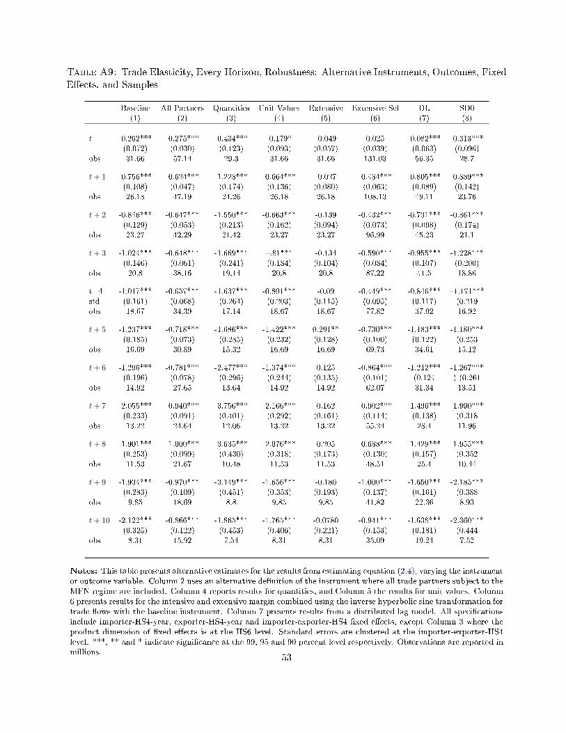
Table A9: Trade Elasticity, Every Horizon, Robustness: Alternative Instruments, Outcomes, FixedE�ects, and Samples

Baseline All Partners Quantities Unit Values Extensive Extensive Sel DL SD0(1) (2) (3) (4) (5) (6) (7) (8)

t -0.262*** -0.275*** -0.434*** -0.179* -0.049 0.025 -0.082*** -0.313***(0.072) (0.030) (0.123) (0.093) (0.057) (0.039) (0.063) (0.096)

obs 31.66 57.14 29.3 31.66 31.66 131.03 56.35 28.7

t+ 1 -0.756*** -0.624*** -1.228*** -0.664*** -0.027 -0.484*** -0.805*** -0.889***(0.108) (0.047) (0.174) (0.136) (0.080) (0.063) (0.089) (0.142)

obs 26.18 47.19 24.26 26.18 26.18 108.13 49.11 23.76

t+ 2 -0.846*** -0.647*** -1.550*** -0.663*** -0.139 -0.432*** -0.731*** -0.861***(0.129) (0.053) (0.213) (0.162) (0.094) (0.073) (0.098) (0.174)

obs 23.27 42.29 21.42 23.27 23.27 96.99 45.23 21.1

t+ 3 -1.024*** -0.648*** -1.669*** �.81*** -0.134 -0.590*** -0.955*** -1.228***(0.146) (0.061) (0.241) (0.184) (0.104) (0.084) (0.107) (0.200)

obs 20.8 38.16 19.14 20.8 20.8 87.22 41.5 18.86

t+4 -1.017*** -0.657*** -1.637*** -0.801*** -0.09 -0.449*** -0.846*** �1.171***std (0.161) (0.068) (0.264) (0.203) (0.115) (0.095) (0.117) (0.219obs 18.67 34.39 17.14 18.67 18.67 77.82 37.92 16.92

t+ 5 -1.237*** -0.718*** -1.686*** -1.422*** 0.291** -0.730*** -1.183*** -1.180***(0.185) (0.073) (0.285) (0.232) (0.128) (0.100) (0.122) (0.253

obs 16.69 30.89 15.32 16.69 16.69 69.73 34.61 15.12

t+ 6 -1.296*** -0.781*** -2.477*** -1.374*** 0.125 -0.864*** -1.212*** -1.267***(0.196) (0.078) (0.296) (0.244) (0.135) (0.101) (0.124 ) (0.261

obs 14.92 27.65 13.64 14.92 14.92 62.07 31.34 13.51

t+ 7 -2.055*** -0.940*** -3.756*** -2.166*** 0.162 -0.902*** -1.496*** -1.990***(0.233) (0.091) (0.401) (0.292) (0.161) (0.114) (0.138) (0.318

obs 13.22 24.64 12.06 13.22 13.22 55.24 28.4 11.96

t+ 8 -1.901*** -1.000*** -3.635*** -2.076*** 0.205 -0.688*** -1.429*** -1.955***(0.253) (0.099) (0.430) (0.318) (0.173) (0.130) (0.157) (0.352

obs 11.53 21.67 10.48 11.53 11.53 48.51 25.4 10.44

t+ 9 -1.934*** -0.970*** -3.149*** -1.656*** -0.180 -1.000*** -1.650*** -2.185***(0.283) (0.109) (0.451) (0.353) (0.193) (0.137) (0.161) (0.388

obs 9.85 18.69 8.8 9.85 9.85 41.82 22.36 8.93

t+ 10 -2.122*** -0.866*** -1.865*** -1.765*** -0.0780 -0.941*** -1.638*** -2.360***(0.325) (0.122) (0.453) (0.406) (0.221) (0.153) (0.181) (0.444

obs 8.31 15.92 7.54 8.31 8.31 35.09 19.24 7.52

Notes: This table presents alternative estimates for the results from estimating equation (2.4), varying the instrumentor outcome variable. Column 2 uses an alternative de�nition of the instrument where all trade partners subject to theMFN regime are included. Column 4 reports results for quantities, and Column 5 the results for unit values. Column6 presents results for the intensive and extensive margin combined using the inverse hyperbolic sine transformation fortrade �ows with the baseline instrument. Column 7 presents results from a distributed lag model. All speci�cationsinclude importer-HS4-year, exporter-HS4-year and importer-exporter-HS4 �xed e�ects, except Column 3 where theproduct dimension of �xed e�ects is at the HS6 level. Standard errors are clustered at the importer-exporter-HS4level. ***, ** and * indicate signi�cance at the 99, 95 and 90 percent level respectively. Observations are reported inmillions.

53

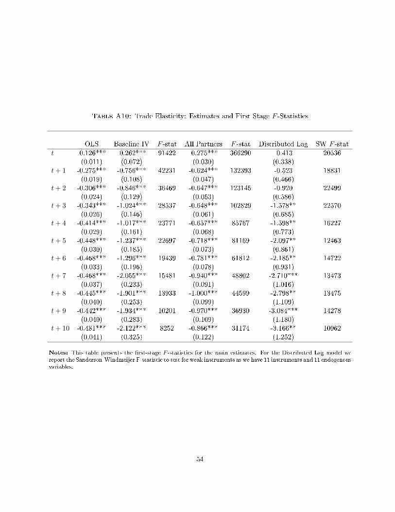
Table A10: Trade Elasticity: Estimates and First Stage F -Statistics

OLS Baseline IV F -stat All Partners F -stat Distributed Lag SW F -statt -0.126*** -0.262*** 91422 -0.275*** 366290 -0.413 20536

(0.011) (0.072) (0.030) (0.338)t+ 1 -0.275*** -0.756*** 42231 -0.624*** 132393 -0.523 18831

(0.019) (0.108) (0.047) (0.466)t+ 2 -0.306*** -0.846*** 36469 -0.647*** 123145 -0.920 22499

(0.024) (0.129) (0.053) (0.586)t+ 3 -0.343*** -1.024*** 28537 -0.648*** 102829 -1.578** 22570

(0.026) (0.146) (0.061) (0.685)t+ 4 -0.414*** -1.017*** 23771 -0.657*** 85767 -1.598** 16227

(0.029) (0.161) (0.068) (0.773)t+ 5 -0.448*** -1.237*** 22697 -0.718*** 81169 -2.097** 12463

(0.030) (0.185) (0.073) (0.861)t+ 6 -0.468*** -1.296*** 19439 -0.781*** 61812 -2.185** 14722

(0.033) (0.196) (0.078) (0.931)t+ 7 -0.468*** -2.055*** 15481 -0.940*** 48802 -2.710*** 13473

(0.037) (0.233) (0.091) (1.016)t+ 8 -0.445*** -1.901*** 13933 -1.000*** 44599 -2.798** 13475

(0.040) (0.253) (0.099) (1.109)t+ 9 -0.442*** -1.934*** 10201 -0.970*** 36930 -3.084*** 14278

(0.040) (0.283) (0.109) (1.180)t+ 10 -0.481*** -2.122*** 8252 -0.866*** 31174 -3.166** 10962

(0.041) (0.325) (0.122) (1.252)

Notes: This table presents the �rst-stage F -statistics for the main estimates. For the Distributed Lag model wereport the Sanderson-Windmeijer F-statistic to test for weak instruments as we have 11 instruments and 11 endogenousvariables.

54

Table A11: Gains from Trade

Country θ̃ = −0.942 θ̃ = −5 θ̃ = −10G7Canada 22.4% 3.9% 1.9%France 16.7% 3.0% 1.5%Germany 21.7% 3.8% 1.9%Italy 14.9% 2.7% 1.3%Japan 8.2% 1.5% 0.7%UK 14.8% 2.6% 1.3%US 5.6% 1.0% 0.5%

Major Emerging MarketsBrazil 7.9% 1.4% 0.7%China 11.9% 2.1% 1.1%India 11.2% 2.0% 1.0%Mexico 6.5% 1.2% 0.6%Russia 20.8% 3.6% 1.8%South Africa 15.0% 2.7% 1.3%

Median, 64 Countries 24.5% 4.2% 2.1%

Notes: Data are from the OECD IO tables for 64 countries in year 2006. Gains from trade relative to autarky are

computed using the formula λ1/θ̃jj , where λjj is 1 minus the import share. The import share is calculated as imports

divided by gross output. The numbers for China and Mexico include export-processing activities (China) and globalmanufacturing activities (Mexico).

55