the market
DESCRIPTION
1. The Market. The Theory of Economics does not furnish a body of settled conclusions immediately applicable to policy. It is a method rather than a doctrine, an apparatus of the mind, a technique of thinking which helps its possessor to draw correct conclusions --- John Maynard Keynes. - PowerPoint PPT PresentationTRANSCRIPT

© 2010 W. W. Norton & Company, Inc.
1 The Market
© 2010 W. W. Norton & Company, Inc. 2
The Theory of Economics does notfurnish a body of settled conclusionsimmediately applicable to policy. It isa method rather than a doctrine, anapparatus of the mind, a technique ofthinking which helps its possessor todraw correct conclusions
--- John Maynard Keynes
© 2010 W. W. Norton & Company, Inc. 3
Economic Modeling
What causes what in economic systems?
At what level of detail shall we model an economic phenomenon?
Which variables are determined outside the model (exogenous) and which are to be determined by the model (endogenous)?
© 2010 W. W. Norton & Company, Inc. 4
Modeling the Apartment Market
How are apartment rents determined? Suppose
– apartments are close or distant, but otherwise identical
– distant apartments rents are exogenous and known
– many potential renters and landlords

© 2010 W. W. Norton & Company, Inc. 5
Modeling the Apartment Market
Who will rent close apartments? At what price? Will the allocation of apartments be
desirable in any sense?
How can we construct an insightful model to answer these questions?
© 2010 W. W. Norton & Company, Inc. 6
Economic Modeling Assumptions
Two basic postulates:
– Rational Choice: Each person tries to choose the best alternative available to him or her.
– Equilibrium: Market price adjusts until quantity demanded equals quantity supplied.

© 2010 W. W. Norton & Company, Inc. 7
Modeling Apartment Demand Demand: Suppose the most any one
person is willing to pay to rent a close apartment is $500/month. Then
p = $500 QD = 1. Suppose the price has to drop to
$490 before a 2nd person would rent. Then p = $490 QD = 2.

© 2010 W. W. Norton & Company, Inc. 8
Modeling Apartment Demand
The lower is the rental rate p, the larger is the quantity of close apartments demanded
p QD . The quantity demanded vs. price
graph is the market demand curve for close apartments.

© 2010 W. W. Norton & Company, Inc. 9
Market Demand Curve for Apartments
p
QD
© 2010 W. W. Norton & Company, Inc. 10
Modeling Apartment Supply
Supply: It takes time to build more close apartments so in this short-run the quantity available is fixed (at say 100).
© 2010 W. W. Norton & Company, Inc. 11
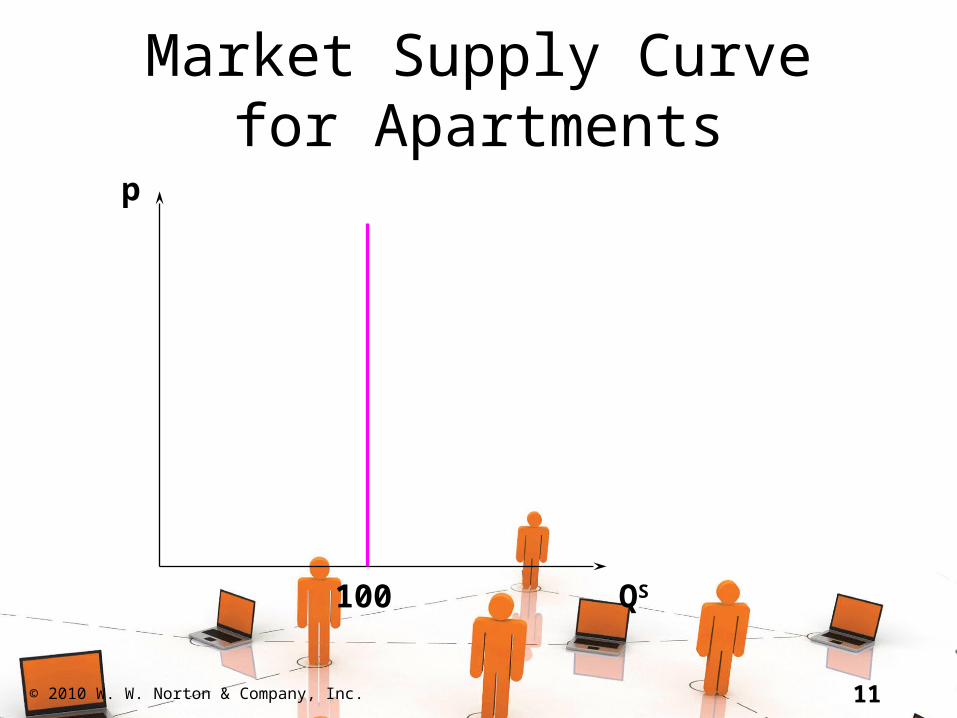
Market Supply Curve for Apartments
p
QS100

© 2010 W. W. Norton & Company, Inc. 12
Competitive Market Equilibrium
“low” rental price quantity demanded of close apartments exceeds quantity available price will rise.
“high” rental price quantity demanded less than quantity available price will fall.

© 2010 W. W. Norton & Company, Inc. 13
Competitive Market Equilibrium
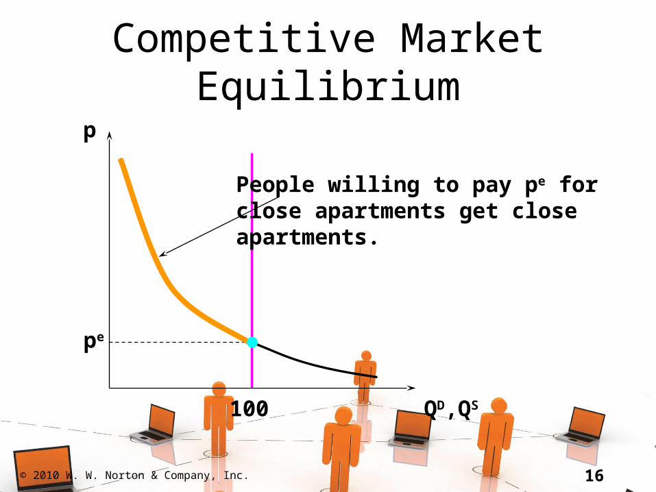
Quantity demanded = quantity available price will neither rise nor fall
so the market is at a competitive equilibrium.

© 2010 W. W. Norton & Company, Inc. 14
Competitive Market Equilibrium
p
QD,QS100

© 2010 W. W. Norton & Company, Inc. 15
Competitive Market Equilibrium
p
QD,QS
pe
100
© 2010 W. W. Norton & Company, Inc. 16
Competitive Market Equilibrium
p
QD,QS
pe
100
People willing to pay pe for close apartments get closeapartments.
© 2010 W. W. Norton & Company, Inc. 17
Competitive Market Equilibrium
p
QD,QS
pe
100
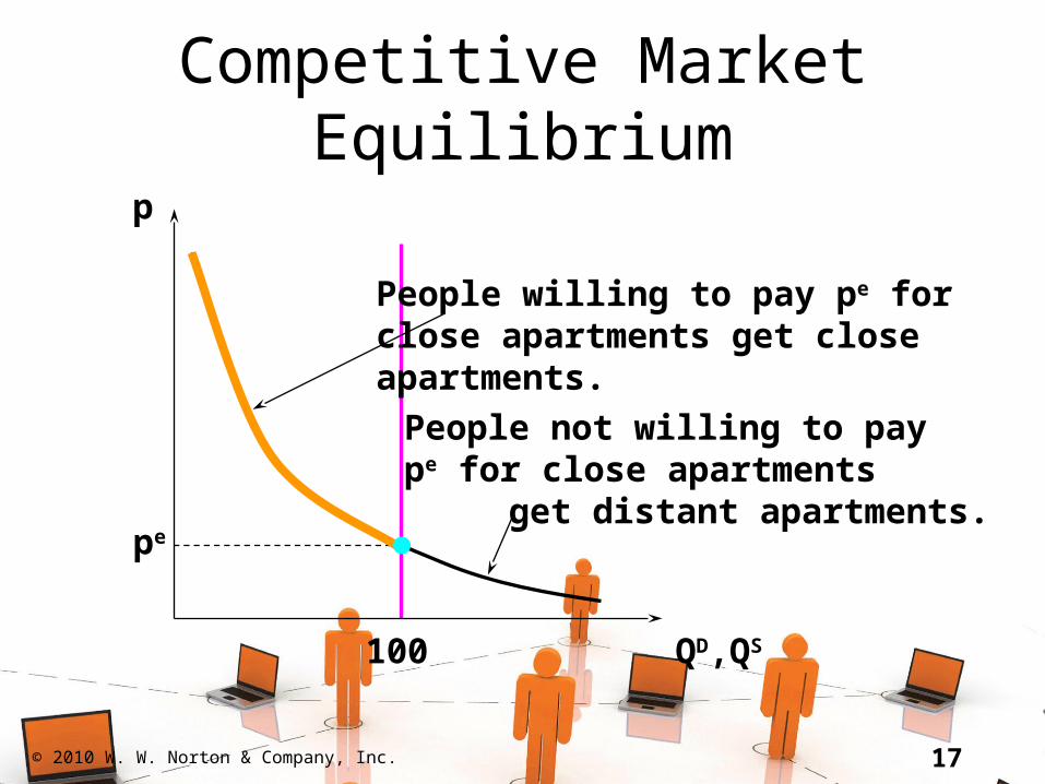
People willing to pay pe for close apartments get closeapartments.
People not willing to pay pe for close apartments get distant apartments.
© 2010 W. W. Norton & Company, Inc. 18
Competitive Market Equilibrium
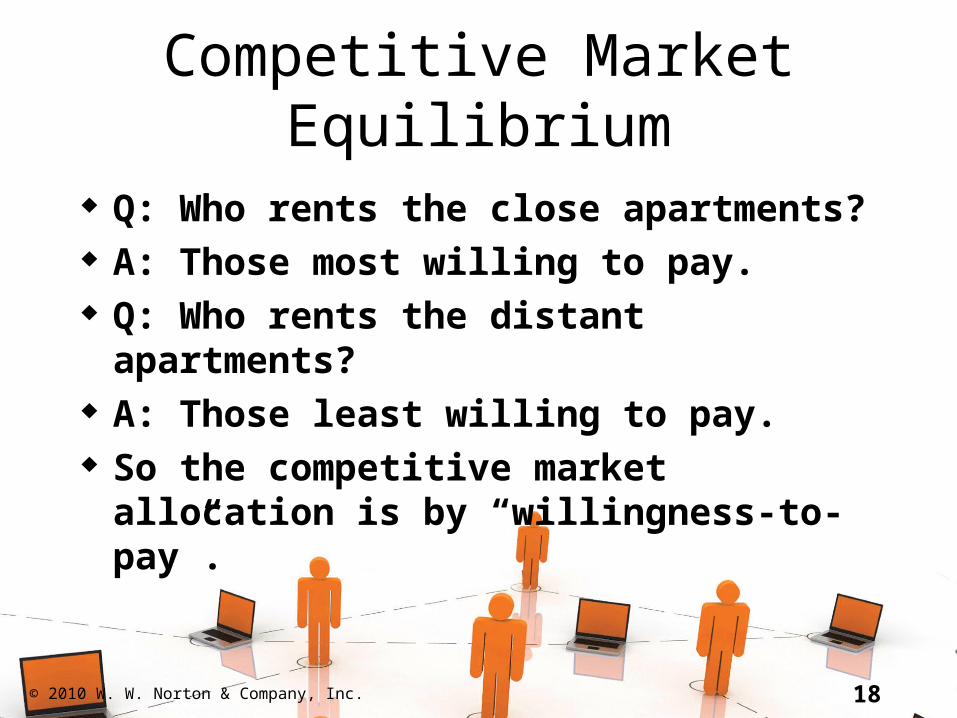
Q: Who rents the close apartments? A: Those most willing to pay. Q: Who rents the distant
apartments? A: Those least willing to pay. So the competitive market allocation
is by “willingness-to-pay”.
© 2010 W. W. Norton & Company, Inc. 19
Comparative Statics
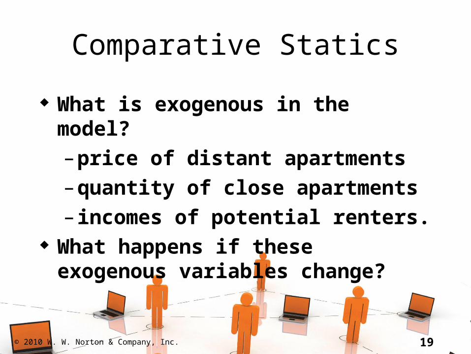
What is exogenous in the model?
– price of distant apartments
– quantity of close apartments
– incomes of potential renters. What happens if these exogenous
variables change?

© 2010 W. W. Norton & Company, Inc. 20
Comparative Statics
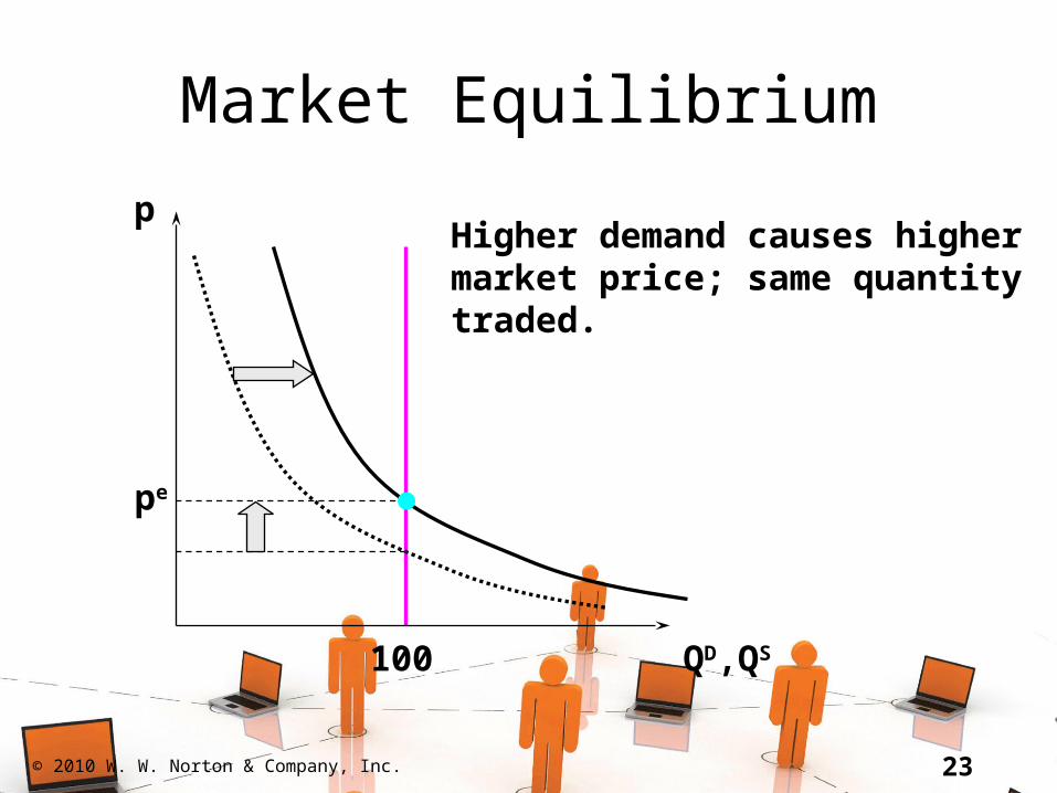
Suppose the price of distant apartment rises.
Demand for close apartments increases (rightward shift), causing a higher price for close apartments.

© 2010 W. W. Norton & Company, Inc. 21
Market Equilibrium
p
QD,QS
pe
100

© 2010 W. W. Norton & Company, Inc. 22
Market Equilibrium
p
QD,QS
pe
100
Higher demand
© 2010 W. W. Norton & Company, Inc. 23
Market Equilibrium
p
QD,QS
pe
100
Higher demand causes highermarket price; same quantitytraded.
© 2010 W. W. Norton & Company, Inc. 24
Comparative Statics
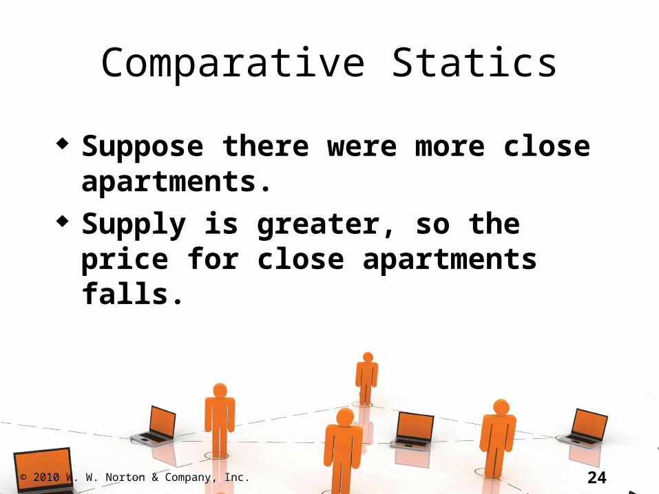
Suppose there were more close apartments.
Supply is greater, so the price for close apartments falls.

© 2010 W. W. Norton & Company, Inc. 25
Market Equilibrium
p
QD,QS
pe
100
© 2010 W. W. Norton & Company, Inc. 26
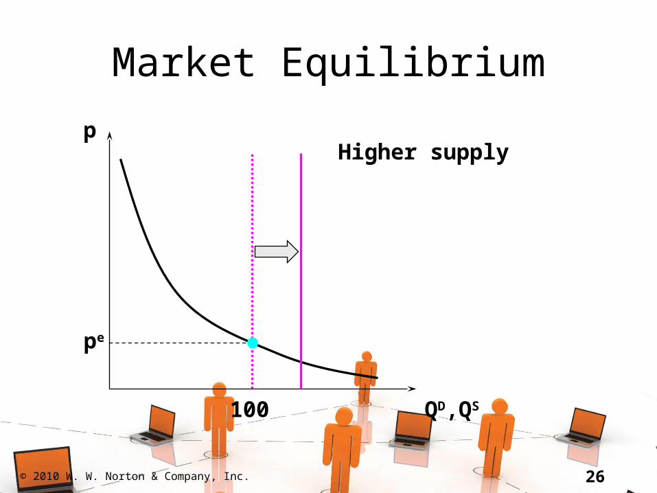
Market Equilibrium
p
QD,QS100
Higher supply
pe

© 2010 W. W. Norton & Company, Inc. 27
Market Equilibrium
p
QD,QS
pe
100
Higher supply causes alower market price and alarger quantity traded.

© 2010 W. W. Norton & Company, Inc. 28
Comparative Statics
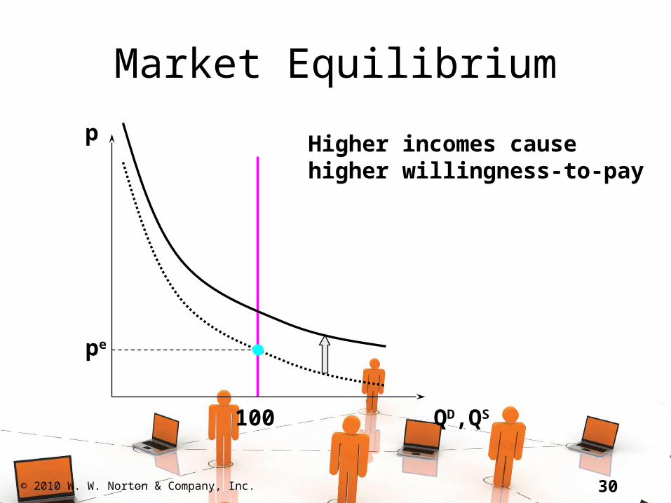
Suppose potential renters’ incomes rise, increasing their willingness-to-pay for close apartments.
Demand rises (upward shift), causing
higher price for close apartments.

© 2010 W. W. Norton & Company, Inc. 29
Market Equilibrium
p
QD,QS
pe
100
© 2010 W. W. Norton & Company, Inc. 30
Market Equilibrium
p
QD,QS
pe
100
Higher incomes causehigher willingness-to-pay
© 2010 W. W. Norton & Company, Inc. 31
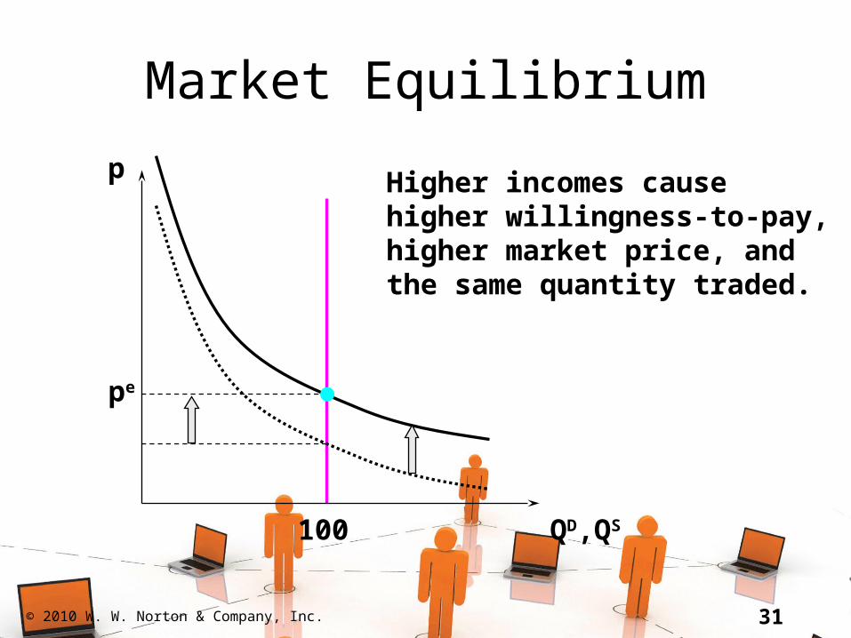
Market Equilibrium
p
QD,QS
pe
100
Higher incomes causehigher willingness-to-pay,higher market price, andthe same quantity traded.

© 2010 W. W. Norton & Company, Inc. 32
Taxation Policy Analysis
Local government taxes apartment owners.
What happens to
– price
– quantity of close apartments rented?
Is any of the tax “passed” to renters?
© 2010 W. W. Norton & Company, Inc. 33
Taxation Policy Analysis Market supply is unaffected. Market demand is unaffected. So the competitive market
equilibrium is unaffected by the tax. Price and the quantity of close
apartments rented are not changed. Landlords pay all of the tax.
© 2010 W. W. Norton & Company, Inc. 34
Imperfectly Competitive Markets
Amongst many possibilities are:
– a monopolistic landlord
– a perfectly discriminatory monopolistic landlord
– a competitive market subject to rent control.
© 2010 W. W. Norton & Company, Inc. 35
A Monopolistic Landlord
When the landlord sets a rental price p he rents D(p) apartments.
Revenue = pD(p). Revenue is low if p 0 Revenue is low if p is so high that
D(p) 0. An intermediate value for p
maximizes revenue.

© 2010 W. W. Norton & Company, Inc. 36
Monopolistic Market Equilibrium
p
QD
Lowprice
Low price, high quantitydemanded, low revenue.

© 2010 W. W. Norton & Company, Inc. 37
Monopolistic Market Equilibrium
p
QD
Highprice
High price, low quantitydemanded, low revenue.
© 2010 W. W. Norton & Company, Inc. 38
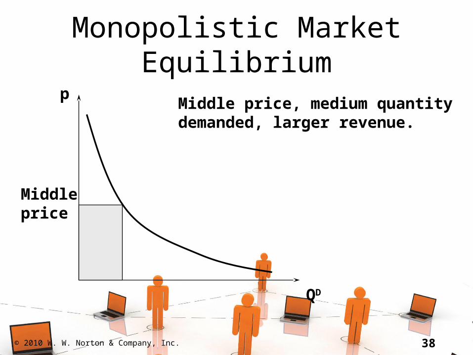
Monopolistic Market Equilibrium
p
QD
Middleprice
Middle price, medium quantitydemanded, larger revenue.

© 2010 W. W. Norton & Company, Inc. 39
Monopolistic Market Equilibrium
p
QD,QS
Middleprice
Middle price, medium quantitydemanded, larger revenue.Monopolist does not rent all theclose apartments.
100
© 2010 W. W. Norton & Company, Inc. 40
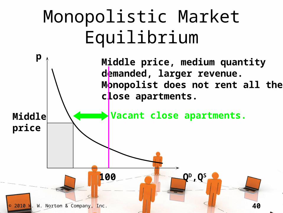
Monopolistic Market Equilibrium
p
QD,QS
Middleprice
Middle price, medium quantitydemanded, larger revenue.Monopolist does not rent all theclose apartments.
100
Vacant close apartments.

© 2010 W. W. Norton & Company, Inc. 41
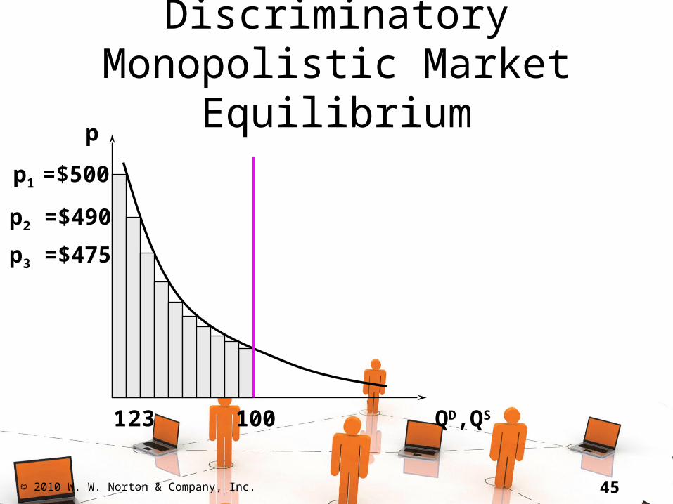
Perfectly Discriminatory Monopolistic Landlord
Imagine the monopolist knew everyone’s willingness-to-pay.
Charge $500 to the most willing-to-pay,
charge $490 to the 2nd most willing-to-pay, etc.

© 2010 W. W. Norton & Company, Inc. 42
Discriminatory Monopolistic Market Equilibrium
p
QD,QS100
p1 =$500
1

© 2010 W. W. Norton & Company, Inc. 43
Discriminatory Monopolistic Market Equilibrium
p
QD,QS100
p1 =$500
p2 =$490
12

© 2010 W. W. Norton & Company, Inc. 44
Discriminatory Monopolistic Market Equilibrium
p
QD,QS100
p1 =$500
p2 =$490
12
p3 =$475
3
© 2010 W. W. Norton & Company, Inc. 45
Discriminatory Monopolistic Market Equilibrium
p
QD,QS100
p1 =$500
p2 =$490
12
p3 =$475
3

© 2010 W. W. Norton & Company, Inc. 46
Discriminatory Monopolistic Market Equilibrium
p
QD,QS100
p1 =$500
p2 =$490
12
p3 =$475
3
pe
Discriminatory monopolistcharges the competitive marketprice to the last renter, andrents the competitive quantityof close apartments.

© 2010 W. W. Norton & Company, Inc. 47
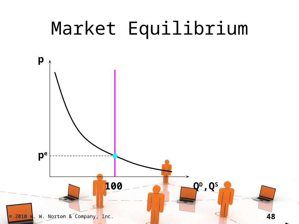
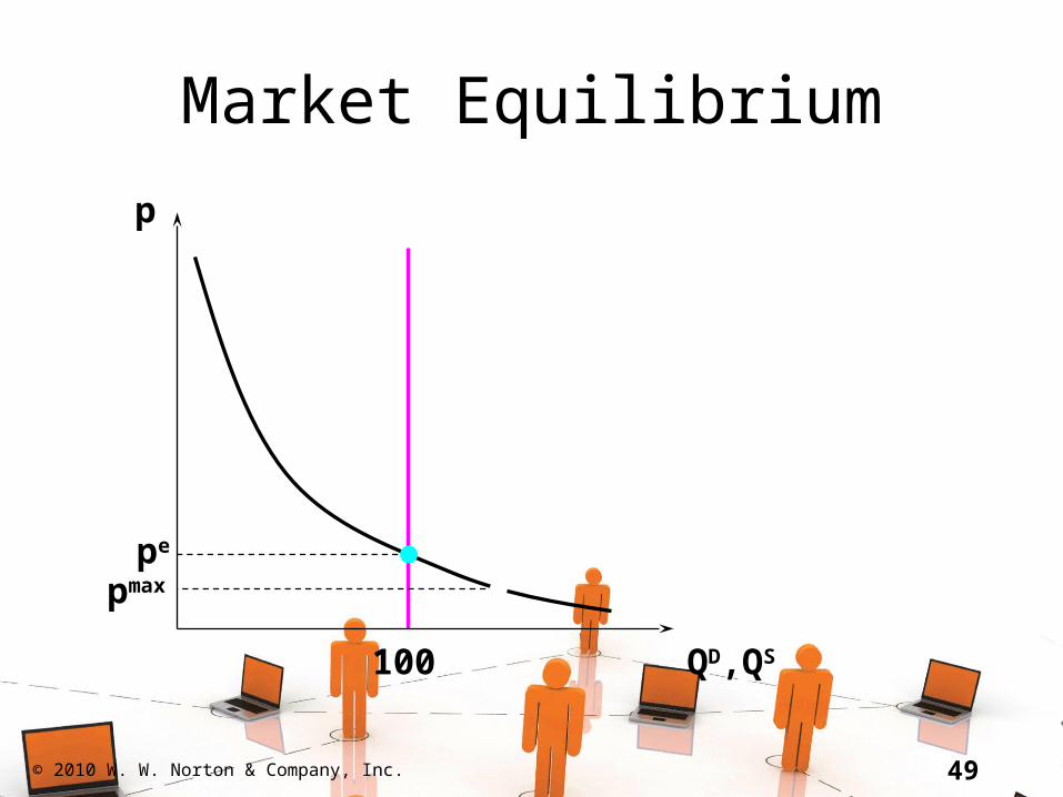
Rent Control
Local government imposes a maximum legal price, pmax < pe, the competitive price.
© 2010 W. W. Norton & Company, Inc. 48
Market Equilibrium
p
QD,QS
pe
100
© 2010 W. W. Norton & Company, Inc. 49
Market Equilibrium
p
QD,QS
pe
100
pmax
© 2010 W. W. Norton & Company, Inc. 50
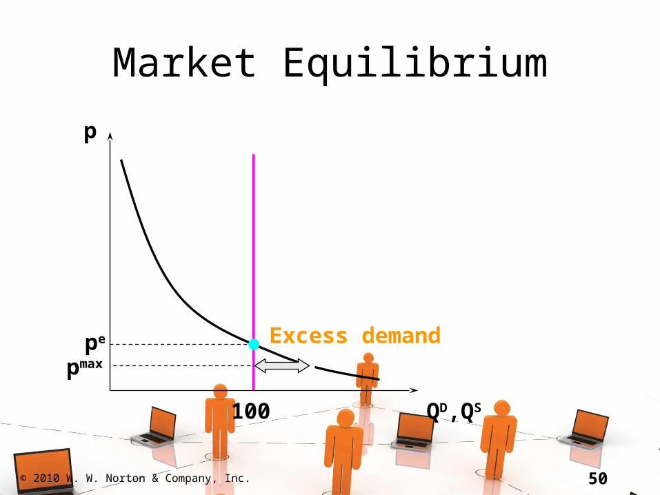
Market Equilibrium
p
QD,QS
pe
100
pmax
Excess demand
© 2010 W. W. Norton & Company, Inc. 51
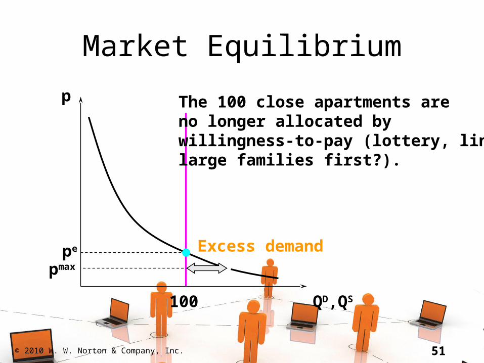
Market Equilibrium
p
QD,QS
pe
100
pmax
Excess demand
The 100 close apartments areno longer allocated bywillingness-to-pay (lottery, lines,large families first?).

© 2010 W. W. Norton & Company, Inc. 52
Which Market Outcomes Are Desirable?
Which is better?
– Rent control
– Perfect competition
– Monopoly
– Discriminatory monopoly
© 2010 W. W. Norton & Company, Inc. 53
Pareto Efficiency
Vilfredo Pareto; 1848-1923. A Pareto outcome allows no “wasted
welfare”; i.e. the only way one person’s
welfare can be improved is to lower another person’s welfare.
© 2010 W. W. Norton & Company, Inc. 54
Pareto Efficiency
Ali has an apartment; Veli does not. Ali values the apartment at $200; Veli
would pay $400 for it. Ali could sublet the apartment to Veli
for $300. Both gain, so it was Pareto inefficient
for Ali to have the apartment.
© 2010 W. W. Norton & Company, Inc. 55
Pareto Efficiency
A Pareto inefficient outcome means there remain unrealized mutual gains-to-trade.
Any market outcome that achieves all possible gains-to-trade must be Pareto efficient.
© 2010 W. W. Norton & Company, Inc. 56
Pareto Efficiency
Competitive equilibrium:
– all close apartment renters value them at the market price pe or more
– all others value close apartments at less than pe
– so no mutually beneficial trades remain
– so the outcome is Pareto efficient.

© 2010 W. W. Norton & Company, Inc. 57
Pareto Efficiency
Discriminatory Monopoly:
– assignment of apartments is the same as with the perfectly competitive market
– so the discriminatory monopoly outcome is also Pareto efficient.

© 2010 W. W. Norton & Company, Inc. 58
Pareto Efficiency
Monopoly:
– not all apartments are occupied
– so a distant apartment renter could be assigned a close apartment and have higher welfare without lowering anybody else’s welfare.
– so the monopoly outcome is Pareto inefficient.
© 2010 W. W. Norton & Company, Inc. 59
Pareto Efficiency
Rent Control:
– some close apartments are assigned to renters valuing them at below the competitive price pe
– some renters valuing a close apartment above pe don’t get close apartments
– Pareto inefficient outcome.