the markovchain package: a package for easily handling
TRANSCRIPT
The markovchain Package: A Package for Easily
Handling Discrete Markov Chains in R
Giorgio Alfredo Spedicato, Tae Seung Kang, and Sai Bhargav Yalamanchi
Abstract
The markovchain package aims to fill a gap within the R framework providing S4 classesand methods for easily handling discrete time Markov chains, homogeneous and simpleinhomogeneous ones. The S4 classes for handling and analysing discrete time Markovchains are presented, as well as functions and method for performing probabilistic andstatistical analysis. Finally, some examples in which the package’s functions are appliedto Economics, Finance and Natural Sciences topics are shown.
Keywords: discrete time Markov chains, transition matrices, communicating classes, period-icity, first passage time, stationary distributions..
1. Introduction
Markov chains represent a class of stochastic processes of great interest for the wide spectrumof practical applications. In particular, discrete time Markov chains (DTMC) permit to modelthe transition probabilities between discrete states by the aid of matrices. Various R packagesdeal with models that are based on Markov chains:
� msm (Jackson 2011) handles Multi-State Models for panel data;
� mcmcR (Geyer and Johnson 2013) implements Monte Carlo Markov Chain approach;
� hmm (Himmelmann and www.linhi.com 2010) fits hidden Markov models with covari-ates;
� mstate fits Multi-State Models based on Markov chains for survival analysis (de Wreede,Fiocco, and Putter 2011).
Nevertheless, the R statistical environment (R Core Team 2013) seems to lack a simple packagethat coherently defines S4 classes for discrete Markov chains and allows to perform probabilis-tic analysis, statistical inference and applications. For the sake of completeness, markovchainis the second package specifically dedicated to DTMC analysis, being DTMCPack (Nicholson2013) the first one. Notwithstanding, markovchain package (Spedicato 2015) aims to offermore flexibility in handling DTMC than other existing solutions, providing S4 classes for bothhomogeneous and non-homogeneous Markov chains as well as methods suited to perform sta-tistical and probabilistic analysis.The markovchain package depends on the following R packages: expm (Goulet, Dutang,Maechler, Firth, Shapira, Stadelmann, and [email protected] 2013)
2 The markovchain package
to perform efficient matrices powers; igraph (Csardi and Nepusz 2006) to perform pretty plot-ting of markovchain objects and matlab (Roebuck 2011), that contains functions for matrixmanagement and calculations that emulate those within MATLAB environment. Moreover,other scientific softwares provide functions specifically designed to analyze DTMC, as Math-ematica 9 (Wolfram Research 2013b).The paper is structured as follows: Section 2 briefly reviews mathematics and definitions re-garding DTMC, Section 3 discusses how to handle and manage Markov chain objects withinthe package, Section 4 and Section 5 show how to perform probabilistic and statistical mod-elling, while Section 6 presents some applied examples from various fields analyzed by meansof the markovchain package.
2. Review of core mathematical concepts
2.1. General Definitions
A DTMC is a sequence of random variables X1, X2 , . . . , Xn, . . . characterized by the Markovproperty (also known as memoryless property, see Equation 1). The Markov property statesthat the distribution of the forthcoming state Xn+1 depends only on the current state Xn
and doesn’t depend on the previous ones Xn−1, Xn−2, . . . , X1.
Pr (Xn+1 = xn+1 |X1 = x1, X2 = x2,..., Xn = xn ) = Pr (Xn+1 = xn+1 |Xn = xn ) . (1)
The set of possible states S = {s1, s2, ..., sr} of Xn can be finite or countable and it is namedthe state space of the chain.
The chain moves from one state to another (this change is named either ’transition’ or ’step’)and the probability pij to move from state si to state sj in one step is named transitionprobability:
pij = Pr (X1 = sj |X0 = si ) . (2)
The probability of moving from state i to j in n steps is denoted by p(n)ij = Pr (Xn = sj |X0 = si ).
A DTMC is called time-homogeneous if the property shown in Equation 3 holds. Timehomogeneity implies no change in the underlying transition probabilities as time goes on.
Pr (Xn+1 = sj |Xn = si ) = Pr (Xn = sj |Xn−1 = si ) . (3)
If the Markov chain is time-homogeneous, then pij = Pr (Xk+1 = sj |Xk = si ) and
p(n)ij = Pr (Xn+k = sj |Xk = si ), where k > 0.
The probability distribution of transitions from one state to another can be represented intoa transition matrix P = (pij)i,j , where each element of position (i, j) represents the transitionprobability pij . E.g., if r = 3 the transition matrix P is shown in Equation 4
P =
p11 p12 p13p21 p22 p23p31 p32 p33
. (4)
Giorgio Alfredo Spedicato, Tae Seung Kang, Sai Bhargav Yalamanchi 3
The distribution over the states can be written in the form of a stochastic row vector x (theterm stochastic means that
∑i xi = 1, xi ≥ 0): e.g., if the current state of x is s2, x = (0 1 0).
As a consequence, the relation between x(1) and x(0) is x(1) = x(0)P and, recursively, we getx(2) = x(0)P 2 and x(n) = x(0)Pn, n > 0.
DTMC are explained in most theory books on stochastic processes, see Bremaud (1999) andChing and Ng (2006) for example. Valuable references online available are: ?, Snell (1999)and Bard (2000).
2.2. Properties and classification of states
A state sj is said accessible from state si (written si → sj) if a system started in state si hasa positive probability to reach the state sj at a certain point, i.e., ∃n > 0 : pnij > 0. If bothsi → sj and sj → si, then si and sj are said to communicate.
A communicating class is defined to be a set of states that communicate. A DTMC can becomposed by one or more communicating classes. If the DTMC is composed by only onecommunicating class (i.e., if all states in the chain communicate), then it is said irreducible.A communicating class is said to be closed if no states outside of the class can be reachedfrom any state inside it.
If pii = 1, si is defined as absorbing state: an absorbing state corresponds to a closed com-municating class composed by one state only.
The canonic form of a DTMC transition matrix is a matrix having a block form, where theclosed communicating classes are shown at the beginning of the diagonal matrix.
A state si has period ki if any return to state si must occur in multiplies of ki steps, that iski = gcd {n : Pr (Xn = si |X0 = si ) > 0}, where gcd is the greatest common divisor. If ki = 1the state si is said to be aperiodic, else if ki > 1 the state si is periodic with period ki. Looselyspeaking, si is periodic if it can only return to itself after a fixed number of transitions ki > 1(or multiple of ki), else it is aperiodic.
If states si and sj belong to the same communicating class, then they have the same periodki. As a consequence, each of the states of an irreducible DTMC share the same periodicity.This periodicity is also considered the DTMC periodicity.
It is possible to analyze the timing to reach a certain state. The first passage time from statesi to state sj is the number Tij of steps taken by the chain until it arrives for the first timeto state sj , given that X0 = si. The probability distribution of Tij is defined by Equation 5
hij(n) = Pr (Tij = n) = Pr (Xn = sj , Xn−1 6= sj , . . . , X1 6= sj |X0 = si) (5)
and can be found recursively using Equation 6, given that hij(n) = pij .
hij(n) =
∑k∈S−{sj}
pikhkj(n−1). (6)
If in the definition of the first passage time we let si = sj , we obtain the first return timeTi = inf{n ≥ 1 : Xn = si|X0 = si}. A state si is said to be recurrent if it is visited infinitelyoften, i.e., Pr(Ti < +∞|X0 = si) = 1. On the opposite, si is called transient if there is apositive probability that the chain will never return to si, i.e., Pr(Ti = +∞|X0 = si) > 0.
4 The markovchain package
Given a time homogeneous Markov chain with transition matrix P, a stationary distributionz is a stochastic row vector such that z = z · P , where 0 ≤ zj ≤ 1 ∀j and
∑j zj = 1.
If a DTMC {Xn} is irreducible and aperiodic, then it has a limit distribution and this distri-bution is stationary. As a consequence, if P is the k × k transition matrix of the chain andz = (z1, ..., zk) is the eigenvector of P such that
∑ki=1 zi = 1, then we get
limn→∞
Pn = Z, (7)
where Z is the matrix having all rows equal to z. The stationary distribution of {Xn} isrepresented by z.
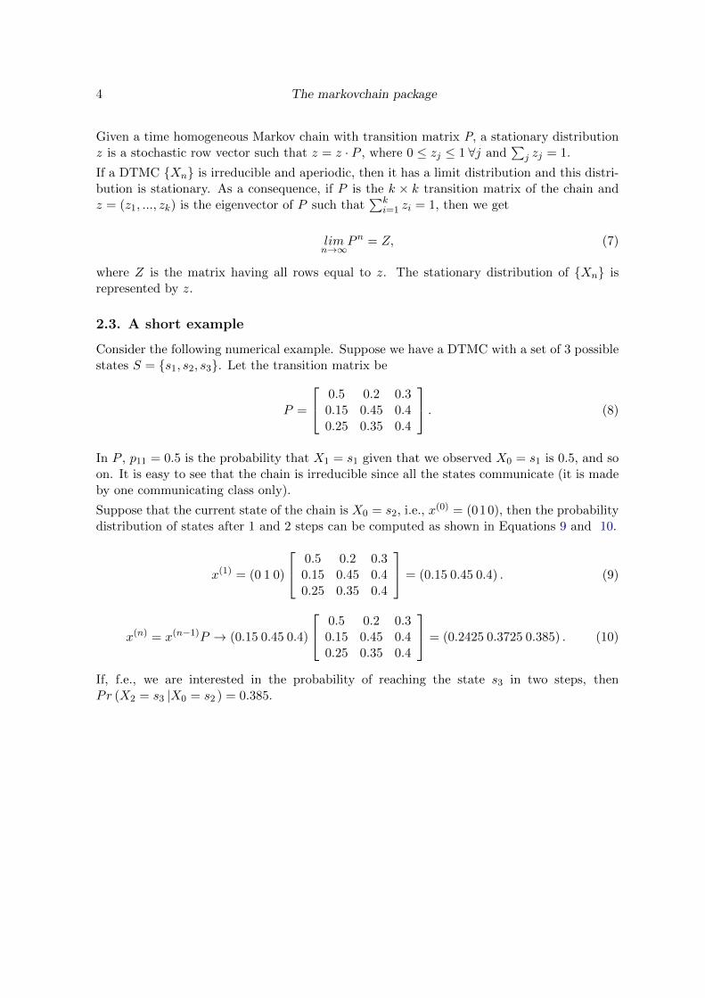
2.3. A short example
Consider the following numerical example. Suppose we have a DTMC with a set of 3 possiblestates S = {s1, s2, s3}. Let the transition matrix be
P =
0.5 0.2 0.30.15 0.45 0.40.25 0.35 0.4
. (8)
In P , p11 = 0.5 is the probability that X1 = s1 given that we observed X0 = s1 is 0.5, and soon. It is easy to see that the chain is irreducible since all the states communicate (it is madeby one communicating class only).
Suppose that the current state of the chain is X0 = s2, i.e., x(0) = (010), then the probabilitydistribution of states after 1 and 2 steps can be computed as shown in Equations 9 and 10.
x(1) = (0 1 0)
0.5 0.2 0.30.15 0.45 0.40.25 0.35 0.4
= (0.15 0.45 0.4) . (9)
x(n) = x(n−1)P → (0.15 0.45 0.4)
0.5 0.2 0.30.15 0.45 0.40.25 0.35 0.4
= (0.2425 0.3725 0.385) . (10)
If, f.e., we are interested in the probability of reaching the state s3 in two steps, thenPr (X2 = s3 |X0 = s2 ) = 0.385.

Giorgio Alfredo Spedicato, Tae Seung Kang, Sai Bhargav Yalamanchi 5
3. The structure of the package
3.1. Creating markovchain objects
The package is loaded within the R command line as follows:
R> library("markovchain")
The markovchain and markovchainList S4 classes (Chambers 2008) are defined within themarkovchain package as displayed:
Class "markovchain" [package "markovchain"]
Slots:
Name: states byrow transitionMatrix
Class: character logical matrix
Name: name
Class: character
Class "markovchainList" [package "markovchain"]
Slots:
Name: markovchains name
Class: list character
The first class has been designed to handle homogeneous Markov chain processes, whilethe latter (which is itself a list of markovchain objects) has been designed to handle non-homogeneous Markov chains processes.
Any element of markovchain class is comprised by following slots:
1. states: a character vector, listing the states for which transition probabilities aredefined.
2. byrow: a logical element, indicating whether transition probabilities are shown by rowor by column.
3. transitionMatrix: the probabilities of the transition matrix.
4. name: optional character element to name the DTMC.
The markovchainList objects are defined by following slots:
1. markovchains: a list of markovchain objects.
2. name: optional character element to name the DTMC.
6 The markovchain package
The markovchain objects can be created either in a long way, as the following code shows
R> weatherStates <- c("sunny", "cloudy", "rain")
R> byRow <- TRUE
R> weatherMatrix <- matrix(data = c(0.70, 0.2, 0.1,
+ 0.3, 0.4, 0.3,
+ 0.2, 0.45, 0.35), byrow = byRow, nrow = 3,
+ dimnames = list(weatherStates, weatherStates))
R> mcWeather <- new("markovchain", states = weatherStates, byrow = byRow,
+ transitionMatrix = weatherMatrix, name = "Weather")
or in a shorter way, displayed below
R> mcWeather <- new("markovchain", states = c("sunny", "cloudy", "rain"),
+ transitionMatrix = matrix(data = c(0.70, 0.2, 0.1,
+ 0.3, 0.4, 0.3,
+ 0.2, 0.45, 0.35), byrow = byRow, nrow = 3),
+ name = "Weather")
When new("markovchain") is called alone, a default Markov chain is created.
R> defaultMc <- new("markovchain")
The quicker way to create markovchain objects is made possible thanks to the implementedinitialize S4 method that checks that:
� the transitionMatrix to be a transition matrix, i.e., all entries to be probabilities andeither all rows or all columns to sum up to one.
� the columns and rows names of transitionMatrix to be defined and to coincide withstates vector slot.
The markovchain objects can be collected in a list within markovchainList S4 objects asfollowing example shows.
R> mcList <- new("markovchainList", markovchains = list(mcWeather, defaultMc),
+ name = "A list of Markov chains")
3.2. Handling markovchain objects
Table 1 lists which methods handle and manipulate markovchain objects.
The examples that follow shows how operations on markovchain objects can be easily per-formed. For example, using the previously defined matrix we can find what is the probabilitydistribution of expected weather states in two and seven days, given the actual state to becloudy.
Giorgio Alfredo Spedicato, Tae Seung Kang, Sai Bhargav Yalamanchi 7
Method Purpose
* Direct multiplication for transition matrices.[ Direct access to the elements of the transition matrix.== Equality operator between two transition matrices.as Operator to convert markovchain objects into data.frame and
table object.dim Dimension of the transition matrix.plot plot method for markovchain objects.print print method for markovchain objects.show show method for markovchain objects.states Name of the transition states.t Transposition operator (which switches byrow slot value and modifies
the transition matrix coherently).
Table 1: markovchain methods for handling markovchain objects.
R> initialState <- c(0, 1, 0)
R> after2Days <- initialState * (mcWeather * mcWeather)
R> after7Days <- initialState * (mcWeather ^ 7)
R> after2Days
sunny cloudy rain
[1,] 0.39 0.355 0.255
R> round(after7Days, 3)
sunny cloudy rain
[1,] 0.462 0.319 0.219
A similar answer could have been obtained defining the vector of probabilities as a columnvector. A column - defined probability matrix could be set up either creating a new matrixor transposing an existing markovchain object thanks to the t method.
R> initialState <- c(0, 1, 0)
R> after2Days <- (t(mcWeather) * t(mcWeather)) * initialState
R> after7Days <- (t(mcWeather) ^ 7) * initialState
R> after2Days
[,1]
sunny 0.390
cloudy 0.355
rain 0.255
R> round(after7Days, 3)
[,1]
sunny 0.462
8 The markovchain package
cloudy 0.319
rain 0.219
Basic methods have been defined for markovchain objects to quickly get states and transitionmatrix dimension.
R> states(mcWeather)
[1] "sunny" "cloudy" "rain"
R> dim(mcWeather)
[1] 3
A direct access to transition probabilities is provided both by transitionProbability methodand ”[” method.
R> transitionProbability(mcWeather, "cloudy", "rain")
[1] 0.3
R> mcWeather[2,3]
[1] 0.3
The transition matrix of a markovchain object can be displayed using print or show methods(the latter being less laconic). Similarly, the underlying transition probability diagram canbe plotted by the use of plot method (as shown in Figure 1) which is based on igraphpackage (Csardi and Nepusz 2006). plot method for markovchain objects is a wrapper ofplot.igraph for igraph S4 objects defined within the igraph package. Additional parameterscan be passed to plot function to control the network graph layout.
R> print(mcWeather)
sunny cloudy rain
sunny 0.7 0.20 0.10
cloudy 0.3 0.40 0.30
rain 0.2 0.45 0.35
R> show(mcWeather)
Weather
A 3 - dimensional discrete Markov Chain with following states
sunny cloudy rain
The transition matrix (by rows) is defined as follows
sunny cloudy rain
sunny 0.7 0.20 0.10
cloudy 0.3 0.40 0.30
rain 0.2 0.45 0.35

Giorgio Alfredo Spedicato, Tae Seung Kang, Sai Bhargav Yalamanchi 9
Weather transition matrix
0.7
0.40.35
0.30.2
0.2
0.45
0.1
0.3
sunny
cloudyrain
Figure 1: Weather example. Markov chain plot.

10 The markovchain package
Import and export from some specific classes is possible, as shown in Figure 2 and in thefollowing code.
R> mcDf <- as(mcWeather, "data.frame")
R> mcNew <- as(mcDf, "markovchain")
R> mcDf
t0 t1 prob
1 sunny sunny 0.70
2 sunny cloudy 0.20
3 sunny rain 0.10
4 cloudy sunny 0.30
5 cloudy cloudy 0.40
6 cloudy rain 0.30
7 rain sunny 0.20
8 rain cloudy 0.45
9 rain rain 0.35
R> mcIgraph <- as(mcWeather, "igraph")
Coerce from matrix method, as the code below shows, represents another approach to createa markovchain method starting from a given squared probability matrix.
R> myMatr<-matrix(c(.1,.8,.1,.2,.6,.2,.3,.4,.3), byrow=TRUE, ncol=3)
R> myMc<-as(myMatr, "markovchain")
R> myMc
Unnamed Markov chain
A 3 - dimensional discrete Markov Chain with following states
s1 s2 s3
The transition matrix (by rows) is defined as follows
s1 s2 s3
s1 0.1 0.8 0.1
s2 0.2 0.6 0.2
s3 0.3 0.4 0.3
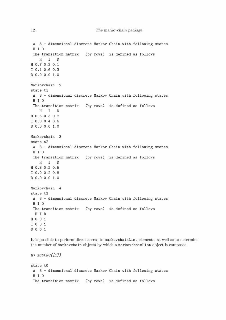
Non-homogeneous Markov chains can be created with the aid of markovchainList object.The example that follows arises from health insurance, where the costs associated to pa-tients in a Continuous Care Health Community (CCHC) are modelled by a non-homogeneousMarkov Chain, since the transition probabilities change by year. Methods explicitly writtenfor markovchainList objects are: print, show, dim and [.
Continuous Care Health Community list of Markov chain(s)
Markovchain 1
state t0
Giorgio Alfredo Spedicato, Tae Seung Kang, Sai Bhargav Yalamanchi 11
Import − Export from and to markovchain objects
dataframe
markovchain
igraph
matrix
table
Figure 2: The markovchain methods for import and export.
12 The markovchain package
A 3 - dimensional discrete Markov Chain with following states
H I D
The transition matrix (by rows) is defined as follows
H I D
H 0.7 0.2 0.1
I 0.1 0.6 0.3
D 0.0 0.0 1.0
Markovchain 2
state t1
A 3 - dimensional discrete Markov Chain with following states
H I D
The transition matrix (by rows) is defined as follows
H I D
H 0.5 0.3 0.2
I 0.0 0.4 0.6
D 0.0 0.0 1.0
Markovchain 3
state t2
A 3 - dimensional discrete Markov Chain with following states
H I D
The transition matrix (by rows) is defined as follows
H I D
H 0.3 0.2 0.5
I 0.0 0.2 0.8
D 0.0 0.0 1.0
Markovchain 4
state t3
A 3 - dimensional discrete Markov Chain with following states
H I D
The transition matrix (by rows) is defined as follows
H I D
H 0 0 1
I 0 0 1
D 0 0 1
It is possible to perform direct access to markovchainList elements, as well as to determinethe number of markovchain objects by which a markovchainList object is composed.
R> mcCCRC[[1]]
state t0
A 3 - dimensional discrete Markov Chain with following states
H I D
The transition matrix (by rows) is defined as follows
Giorgio Alfredo Spedicato, Tae Seung Kang, Sai Bhargav Yalamanchi 13
H I D
H 0.7 0.2 0.1
I 0.1 0.6 0.3
D 0.0 0.0 1.0
R> dim(mcCCRC)
[1] 4
The markovchain package contains some data found in the literature related to DTMC models(see Section 6). Table 2 lists datasets and tables included within the current release of thepackage.
Dataset Description
blanden Mobility across income quartiles, Jo Blanden and Machin (2005).craigsendi CD4 cells, B. A. Craig and A. A. Sendi (2002).preproglucacon Preproglucacon DNA basis, P. J. Avery and D. A. Henderson (1999).rain Alofi Island rains, P. J. Avery and D. A. Henderson (1999).holson Individual states trajectiories.
Table 2: The markovchain data.frame and table.
Finally, Table 3 lists the demos included in the demo directory of the package.
Dataset Description
bard.R Structural analysis of Markov chains from Bard PPT.examples.R Notable Markov chains, e.g., The Gambler Ruin chain.quickStart.R Generic examples.
Table 3: The markovchain demos.
14 The markovchain package
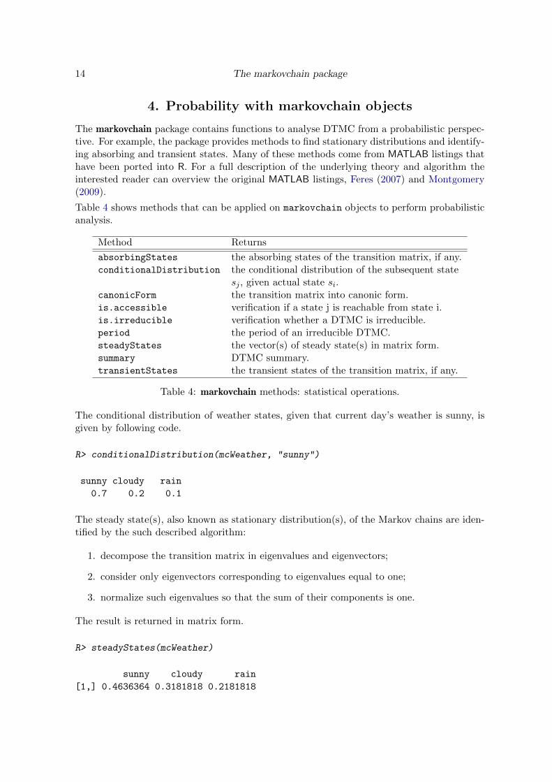
4. Probability with markovchain objects
The markovchain package contains functions to analyse DTMC from a probabilistic perspec-tive. For example, the package provides methods to find stationary distributions and identify-ing absorbing and transient states. Many of these methods come from MATLAB listings thathave been ported into R. For a full description of the underlying theory and algorithm theinterested reader can overview the original MATLAB listings, Feres (2007) and Montgomery(2009).
Table 4 shows methods that can be applied on markovchain objects to perform probabilisticanalysis.
Method Returns
absorbingStates the absorbing states of the transition matrix, if any.conditionalDistribution the conditional distribution of the subsequent state
sj , given actual state si.canonicForm the transition matrix into canonic form.is.accessible verification if a state j is reachable from state i.is.irreducible verification whether a DTMC is irreducible.period the period of an irreducible DTMC.steadyStates the vector(s) of steady state(s) in matrix form.summary DTMC summary.transientStates the transient states of the transition matrix, if any.
Table 4: markovchain methods: statistical operations.
The conditional distribution of weather states, given that current day’s weather is sunny, isgiven by following code.
R> conditionalDistribution(mcWeather, "sunny")
sunny cloudy rain
0.7 0.2 0.1
The steady state(s), also known as stationary distribution(s), of the Markov chains are iden-tified by the such described algorithm:
1. decompose the transition matrix in eigenvalues and eigenvectors;
2. consider only eigenvectors corresponding to eigenvalues equal to one;
3. normalize such eigenvalues so that the sum of their components is one.
The result is returned in matrix form.
R> steadyStates(mcWeather)
sunny cloudy rain
[1,] 0.4636364 0.3181818 0.2181818
Giorgio Alfredo Spedicato, Tae Seung Kang, Sai Bhargav Yalamanchi 15
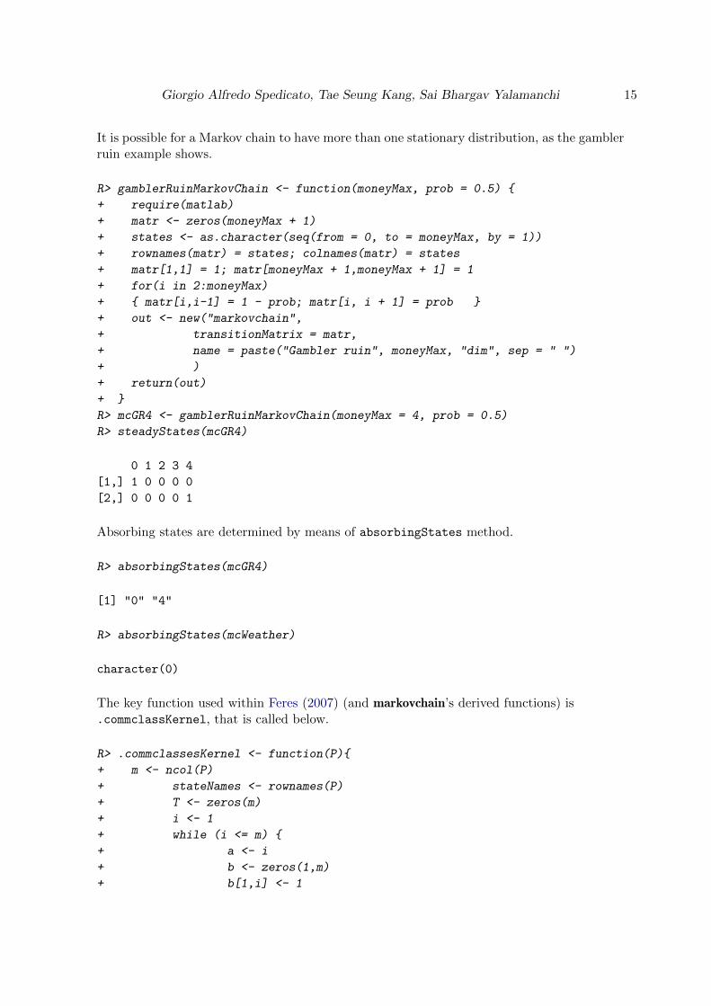
It is possible for a Markov chain to have more than one stationary distribution, as the gamblerruin example shows.
R> gamblerRuinMarkovChain <- function(moneyMax, prob = 0.5) {
+ require(matlab)
+ matr <- zeros(moneyMax + 1)
+ states <- as.character(seq(from = 0, to = moneyMax, by = 1))
+ rownames(matr) = states; colnames(matr) = states
+ matr[1,1] = 1; matr[moneyMax + 1,moneyMax + 1] = 1
+ for(i in 2:moneyMax)
+ { matr[i,i-1] = 1 - prob; matr[i, i + 1] = prob }
+ out <- new("markovchain",
+ transitionMatrix = matr,
+ name = paste("Gambler ruin", moneyMax, "dim", sep = " ")
+ )
+ return(out)
+ }
R> mcGR4 <- gamblerRuinMarkovChain(moneyMax = 4, prob = 0.5)
R> steadyStates(mcGR4)
0 1 2 3 4
[1,] 1 0 0 0 0
[2,] 0 0 0 0 1
Absorbing states are determined by means of absorbingStates method.
R> absorbingStates(mcGR4)
[1] "0" "4"
R> absorbingStates(mcWeather)
character(0)
The key function used within Feres (2007) (and markovchain’s derived functions) is.commclassKernel, that is called below.
R> .commclassesKernel <- function(P){
+ m <- ncol(P)
+ stateNames <- rownames(P)
+ T <- zeros(m)
+ i <- 1
+ while (i <= m) {
+ a <- i
+ b <- zeros(1,m)
+ b[1,i] <- 1
16 The markovchain package
+ old <- 1
+ new <- 0
+ while (old != new) {
+ old <- sum(find(b > 0))
+ n <- size(a)[2]
+ matr <- matrix(as.numeric(P[a,]), ncol = m,
+ nrow = n)
+ c <- colSums(matr)
+ d <- find(c)
+ n <- size(d)[2]
+ b[1,d] <- ones(1,n)
+ new <- sum(find(b>0))
+ a <- d
+ }
+ T[i,] <- b
+ i <- i+1 }
+ F <- t(T)
+ C <- (T > 0)&(F > 0)
+ v <- (apply(t(C) == t(T), 2, sum) == m)
+ colnames(C) <- stateNames
+ rownames(C) <- stateNames
+ names(v) <- stateNames
+ out <- list(C = C, v = v)
+ return(out)
+ }
The .commclassKernel function gets a transition matrix of dimension n and return a list oftwo items:
1. C, an adjacency matrix showing for each state sj (in the row) which states lie in thesame communicating class of sj (flagged with 1).
2. v, a binary vector indicating whether the state sj is transient (0) or not (1).
These functions are used by two other internal functions on which the summary method formarkovchain objects works.
The example matrix used in Feres (2007) well exemplifies the purpose of the function.
R> P <- matlab::zeros(10)
R> P[1, c(1, 3)] <- 1/2;
R> P[2, 2] <- 1/3; P[2,7] <- 2/3;
R> P[3, 1] <- 1;
R> P[4, 5] <- 1;
R> P[5, c(4, 5, 9)] <- 1/3;
R> P[6, 6] <- 1;
R> P[7, 7] <- 1/4; P[7,9] <- 3/4;
R> P[8, c(3, 4, 8, 10)] <- 1/4;

Giorgio Alfredo Spedicato, Tae Seung Kang, Sai Bhargav Yalamanchi 17
R> P[9, 2] <- 1;
R> P[10, c(2, 5, 10)] <- 1/3;
R> rownames(P) <- letters[1:10]
R> colnames(P) <- letters[1:10]
R> probMc <- new("markovchain", transitionMatrix = P,
+ name = "Probability MC")
R> .commclassesKernel(P)
$C
a b c d e f g h i j
a TRUE FALSE TRUE FALSE FALSE FALSE FALSE FALSE FALSE FALSE
b FALSE TRUE FALSE FALSE FALSE FALSE TRUE FALSE TRUE FALSE
c TRUE FALSE TRUE FALSE FALSE FALSE FALSE FALSE FALSE FALSE
d FALSE FALSE FALSE TRUE TRUE FALSE FALSE FALSE FALSE FALSE
e FALSE FALSE FALSE TRUE TRUE FALSE FALSE FALSE FALSE FALSE
f FALSE FALSE FALSE FALSE FALSE TRUE FALSE FALSE FALSE FALSE
g FALSE TRUE FALSE FALSE FALSE FALSE TRUE FALSE TRUE FALSE
h FALSE FALSE FALSE FALSE FALSE FALSE FALSE TRUE FALSE FALSE
i FALSE TRUE FALSE FALSE FALSE FALSE TRUE FALSE TRUE FALSE
j FALSE FALSE FALSE FALSE FALSE FALSE FALSE FALSE FALSE TRUE
$v
a b c d e f g h i j
TRUE TRUE TRUE FALSE FALSE TRUE TRUE FALSE TRUE FALSE
R> summary(probMc)
Probability MC Markov chain that is composed by:
Closed classes:
a c
b g i
f
Transient classes:
d e
h
j
The Markov chain is not irreducible
The absorbing states are: f
All states that pertain to a transient class are named ”transient” and a specific method hasbeen written to elicit them.
R> transientStates(probMc)
[1] "d" "e" "h" "j"
Listings from Feres (2007) have been adapted into canonicForm method that turns a Markovchain into canonic form.

18 The markovchain package
R> probMcCanonic <- canonicForm(probMc)
R> probMc
Probability MC
A 10 - dimensional discrete Markov Chain with following states
a b c d e f g h i j
The transition matrix (by rows) is defined as follows
a b c d e f g h i
a 0.5 0.0000000 0.50 0.0000000 0.0000000 0 0.0000000 0.00 0.0000000
b 0.0 0.3333333 0.00 0.0000000 0.0000000 0 0.6666667 0.00 0.0000000
c 1.0 0.0000000 0.00 0.0000000 0.0000000 0 0.0000000 0.00 0.0000000
d 0.0 0.0000000 0.00 0.0000000 1.0000000 0 0.0000000 0.00 0.0000000
e 0.0 0.0000000 0.00 0.3333333 0.3333333 0 0.0000000 0.00 0.3333333
f 0.0 0.0000000 0.00 0.0000000 0.0000000 1 0.0000000 0.00 0.0000000
g 0.0 0.0000000 0.00 0.0000000 0.0000000 0 0.2500000 0.00 0.7500000
h 0.0 0.0000000 0.25 0.2500000 0.0000000 0 0.0000000 0.25 0.0000000
i 0.0 1.0000000 0.00 0.0000000 0.0000000 0 0.0000000 0.00 0.0000000
j 0.0 0.3333333 0.00 0.0000000 0.3333333 0 0.0000000 0.00 0.0000000
j
a 0.0000000
b 0.0000000
c 0.0000000
d 0.0000000
e 0.0000000
f 0.0000000
g 0.0000000
h 0.2500000
i 0.0000000
j 0.3333333
R> probMcCanonic
Probability MC
A 10 - dimensional discrete Markov Chain with following states
a c b g i f d e h j
The transition matrix (by rows) is defined as follows
a c b g i f d e h
a 0.5 0.50 0.0000000 0.0000000 0.0000000 0 0.0000000 0.0000000 0.00
c 1.0 0.00 0.0000000 0.0000000 0.0000000 0 0.0000000 0.0000000 0.00
b 0.0 0.00 0.3333333 0.6666667 0.0000000 0 0.0000000 0.0000000 0.00
g 0.0 0.00 0.0000000 0.2500000 0.7500000 0 0.0000000 0.0000000 0.00
i 0.0 0.00 1.0000000 0.0000000 0.0000000 0 0.0000000 0.0000000 0.00
f 0.0 0.00 0.0000000 0.0000000 0.0000000 1 0.0000000 0.0000000 0.00
d 0.0 0.00 0.0000000 0.0000000 0.0000000 0 0.0000000 1.0000000 0.00
e 0.0 0.00 0.0000000 0.0000000 0.3333333 0 0.3333333 0.3333333 0.00
h 0.0 0.25 0.0000000 0.0000000 0.0000000 0 0.2500000 0.0000000 0.25
j 0.0 0.00 0.3333333 0.0000000 0.0000000 0 0.0000000 0.3333333 0.00
Giorgio Alfredo Spedicato, Tae Seung Kang, Sai Bhargav Yalamanchi 19
j
a 0.0000000
c 0.0000000
b 0.0000000
g 0.0000000
i 0.0000000
f 0.0000000
d 0.0000000
e 0.0000000
h 0.2500000
j 0.3333333
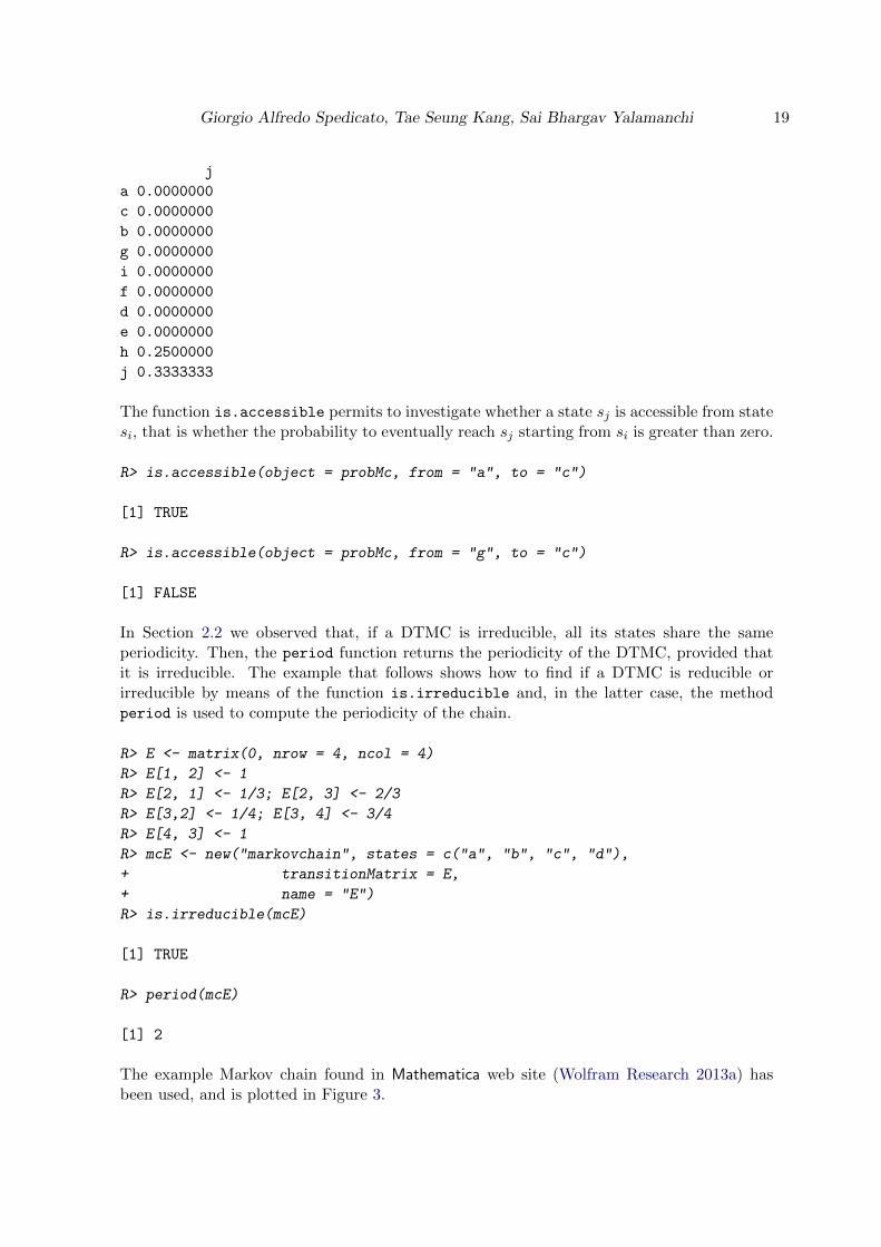
The function is.accessible permits to investigate whether a state sj is accessible from statesi, that is whether the probability to eventually reach sj starting from si is greater than zero.
R> is.accessible(object = probMc, from = "a", to = "c")
[1] TRUE
R> is.accessible(object = probMc, from = "g", to = "c")
[1] FALSE
In Section 2.2 we observed that, if a DTMC is irreducible, all its states share the sameperiodicity. Then, the period function returns the periodicity of the DTMC, provided thatit is irreducible. The example that follows shows how to find if a DTMC is reducible orirreducible by means of the function is.irreducible and, in the latter case, the methodperiod is used to compute the periodicity of the chain.
R> E <- matrix(0, nrow = 4, ncol = 4)
R> E[1, 2] <- 1
R> E[2, 1] <- 1/3; E[2, 3] <- 2/3
R> E[3,2] <- 1/4; E[3, 4] <- 3/4
R> E[4, 3] <- 1
R> mcE <- new("markovchain", states = c("a", "b", "c", "d"),
+ transitionMatrix = E,
+ name = "E")
R> is.irreducible(mcE)
[1] TRUE
R> period(mcE)
[1] 2
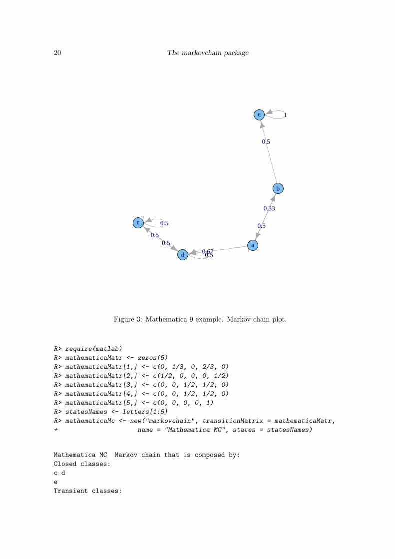
The example Markov chain found in Mathematica web site (Wolfram Research 2013a) hasbeen used, and is plotted in Figure 3.
20 The markovchain package
0.5
0.5
1
0.5
0.33
0.5
0.670.5
0.5
a
b
c
d
e
Figure 3: Mathematica 9 example. Markov chain plot.
R> require(matlab)
R> mathematicaMatr <- zeros(5)
R> mathematicaMatr[1,] <- c(0, 1/3, 0, 2/3, 0)
R> mathematicaMatr[2,] <- c(1/2, 0, 0, 0, 1/2)
R> mathematicaMatr[3,] <- c(0, 0, 1/2, 1/2, 0)
R> mathematicaMatr[4,] <- c(0, 0, 1/2, 1/2, 0)
R> mathematicaMatr[5,] <- c(0, 0, 0, 0, 1)
R> statesNames <- letters[1:5]
R> mathematicaMc <- new("markovchain", transitionMatrix = mathematicaMatr,
+ name = "Mathematica MC", states = statesNames)
Mathematica MC Markov chain that is composed by:
Closed classes:
c d
e
Transient classes:
Giorgio Alfredo Spedicato, Tae Seung Kang, Sai Bhargav Yalamanchi 21
a b
The Markov chain is not irreducible
The absorbing states are: e
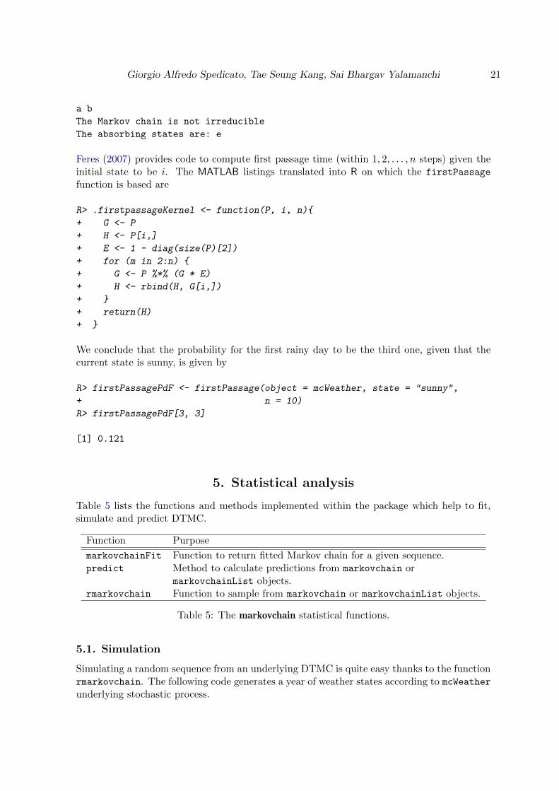
Feres (2007) provides code to compute first passage time (within 1, 2, . . . , n steps) given theinitial state to be i. The MATLAB listings translated into R on which the firstPassage
function is based are
R> .firstpassageKernel <- function(P, i, n){
+ G <- P
+ H <- P[i,]
+ E <- 1 - diag(size(P)[2])
+ for (m in 2:n) {
+ G <- P %*% (G * E)
+ H <- rbind(H, G[i,])
+ }
+ return(H)
+ }
We conclude that the probability for the first rainy day to be the third one, given that thecurrent state is sunny, is given by
R> firstPassagePdF <- firstPassage(object = mcWeather, state = "sunny",
+ n = 10)
R> firstPassagePdF[3, 3]
[1] 0.121
5. Statistical analysis
Table 5 lists the functions and methods implemented within the package which help to fit,simulate and predict DTMC.
Function Purpose
markovchainFit Function to return fitted Markov chain for a given sequence.predict Method to calculate predictions from markovchain or
markovchainList objects.rmarkovchain Function to sample from markovchain or markovchainList objects.
Table 5: The markovchain statistical functions.
5.1. Simulation
Simulating a random sequence from an underlying DTMC is quite easy thanks to the functionrmarkovchain. The following code generates a year of weather states according to mcWeather
underlying stochastic process.
22 The markovchain package
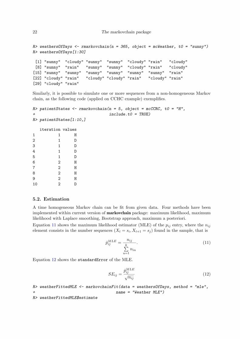
R> weathersOfDays <- rmarkovchain(n = 365, object = mcWeather, t0 = "sunny")
R> weathersOfDays[1:30]
[1] "sunny" "cloudy" "sunny" "sunny" "cloudy" "rain" "cloudy"
[8] "sunny" "rain" "sunny" "sunny" "cloudy" "rain" "cloudy"
[15] "sunny" "sunny" "sunny" "sunny" "sunny" "sunny" "rain"
[22] "cloudy" "rain" "cloudy" "cloudy" "rain" "cloudy" "rain"
[29] "cloudy" "rain"
Similarly, it is possible to simulate one or more sequences from a non-homogeneous Markovchain, as the following code (applied on CCHC example) exemplifies.
R> patientStates <- rmarkovchain(n = 5, object = mcCCRC, t0 = "H",
+ include.t0 = TRUE)
R> patientStates[1:10,]
iteration values
1 1 H
2 1 D
3 1 D
4 1 D
5 1 D
6 2 H
7 2 H
8 2 H
9 2 H
10 2 D
5.2. Estimation
A time homogeneous Markov chain can be fit from given data. Four methods have beenimplemented within current version of markovchain package: maximum likelihood, maximumlikelihood with Laplace smoothing, Bootstrap approach, maximum a posteriori.
Equation 11 shows the maximum likelihood estimator (MLE) of the pij entry, where the nijelement consists in the number sequences (Xt = si, Xt+1 = sj) found in the sample, that is
pMLEij =
nijk∑
u=1niu
. (11)
Equation 12 shows the standardError of the MLE.
SEij =pMLEij√nij
(12)
R> weatherFittedMLE <- markovchainFit(data = weathersOfDays, method = "mle",
+ name = "Weather MLE")
R> weatherFittedMLE$estimate
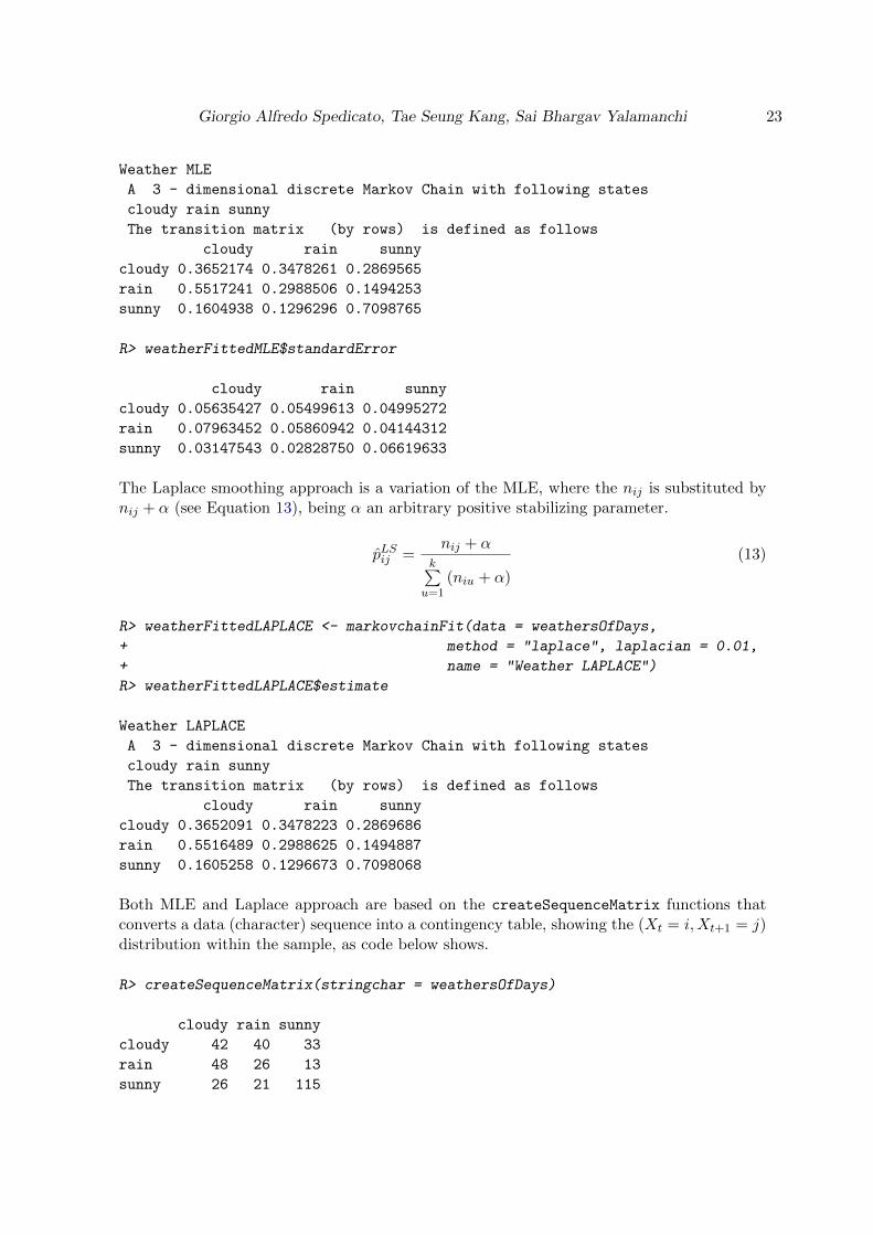
Giorgio Alfredo Spedicato, Tae Seung Kang, Sai Bhargav Yalamanchi 23
Weather MLE
A 3 - dimensional discrete Markov Chain with following states
cloudy rain sunny
The transition matrix (by rows) is defined as follows
cloudy rain sunny
cloudy 0.3652174 0.3478261 0.2869565
rain 0.5517241 0.2988506 0.1494253
sunny 0.1604938 0.1296296 0.7098765
R> weatherFittedMLE$standardError
cloudy rain sunny
cloudy 0.05635427 0.05499613 0.04995272
rain 0.07963452 0.05860942 0.04144312
sunny 0.03147543 0.02828750 0.06619633
The Laplace smoothing approach is a variation of the MLE, where the nij is substituted bynij + α (see Equation 13), being α an arbitrary positive stabilizing parameter.
pLSij =nij + α
k∑u=1
(niu + α)
(13)
R> weatherFittedLAPLACE <- markovchainFit(data = weathersOfDays,
+ method = "laplace", laplacian = 0.01,
+ name = "Weather LAPLACE")
R> weatherFittedLAPLACE$estimate
Weather LAPLACE
A 3 - dimensional discrete Markov Chain with following states
cloudy rain sunny
The transition matrix (by rows) is defined as follows
cloudy rain sunny
cloudy 0.3652091 0.3478223 0.2869686
rain 0.5516489 0.2988625 0.1494887
sunny 0.1605258 0.1296673 0.7098068
Both MLE and Laplace approach are based on the createSequenceMatrix functions thatconverts a data (character) sequence into a contingency table, showing the (Xt = i,Xt+1 = j)distribution within the sample, as code below shows.
R> createSequenceMatrix(stringchar = weathersOfDays)
cloudy rain sunny
cloudy 42 40 33
rain 48 26 13
sunny 26 21 115

24 The markovchain package
An issue occurs when the sample contains only one realization of a state (say Xβ) which islocated at the end of the data sequence, since it yields to a row of zero (no sample to estimatethe conditional distribution of the transition). In this case the estimated transition matrix iscorrected assuming pβ,j = 1/k, being k the possible states.
A bootstrap estimation approach has been developed within the package in order to providean indication of the variability of pij estimates. The bootstrap approach implemented withinthe markovchain package follows these steps:
1. bootstrap the data sequences following the conditional distributions of states estimatedfrom the original one. The default bootstrap samples is 10, as specified in nboot pa-rameter of markovchainFit function.
2. apply MLE estimation on bootstrapped data sequences that are saved inbootStrapSamples slot of the returned list.
3. the pBOOTSTRAP ij is the average of all pMLEij across the bootStrapSamples list, nor-
malized by row. A standardError of ˆpMLEij estimate is provided as well.
R> weatherFittedBOOT <- markovchainFit(data = weathersOfDays,
+ method = "bootstrap", nboot = 100)
R> weatherFittedBOOT$estimate
BootStrap Estimate
A 3 - dimensional discrete Markov Chain with following states
cloudy rain sunny
The transition matrix (by rows) is defined as follows
cloudy rain sunny
cloudy 0.3679941 0.3499262 0.2820796
rain 0.5469893 0.3000676 0.1529431
sunny 0.1585844 0.1316045 0.7098111
R> weatherFittedBOOT$standardError
cloudy rain sunny
cloudy 0.004395227 0.004305609 0.003707920
rain 0.005762406 0.005241380 0.003929288
sunny 0.002853011 0.002808520 0.003823990
For all the methods, the logLikelihood denoted in Equation 14 is provided.
LLH =∑i,j
nij ∗ log(pij) (14)
where nij is the entry of the frequency matrix and pij is the entry of the transition probabilitymatrix.
R> weatherFittedMLE <- markovchainFit(data = weathersOfDays, method = "mle",
+ name = "Weather MLE")
R> weatherFittedMLE$logLikelihood
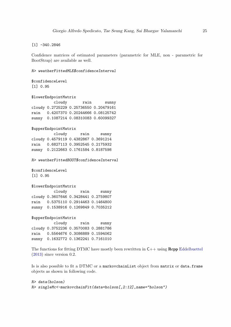
Giorgio Alfredo Spedicato, Tae Seung Kang, Sai Bhargav Yalamanchi 25
[1] -340.2846
Confidence matrices of estimated parameters (parametric for MLE, non - parametric forBootStrap) are available as well.
R> weatherFittedMLE$confidenceInterval
$confidenceLevel
[1] 0.95
$lowerEndpointMatrix
cloudy rain sunny
cloudy 0.2725229 0.25736550 0.20479161
rain 0.4207370 0.20244666 0.08125742
sunny 0.1087214 0.08310083 0.60099327
$upperEndpointMatrix
cloudy rain sunny
cloudy 0.4579119 0.4382867 0.3691214
rain 0.6827113 0.3952545 0.2175932
sunny 0.2122663 0.1761584 0.8187598
R> weatherFittedBOOT$confidenceInterval
$confidenceLevel
[1] 0.95
$lowerEndpointMatrix
cloudy rain sunny
cloudy 0.3607646 0.3428441 0.2759807
rain 0.5375110 0.2914463 0.1464800
sunny 0.1538916 0.1269849 0.7035212
$upperEndpointMatrix
cloudy rain sunny
cloudy 0.3752236 0.3570083 0.2881786
rain 0.5564676 0.3086889 0.1594062
sunny 0.1632772 0.1362241 0.7161010
The functions for fitting DTMC have mostly been rewritten in C++ using Rcpp Eddelbuettel(2013) since version 0.2.
Is is also possible to fit a DTMC or a markovchainList object from matrix or data.frame
objects as shown in following code.
R> data(holson)
R> singleMc<-markovchainFit(data=holson[,2:12],name="holson")
26 The markovchain package
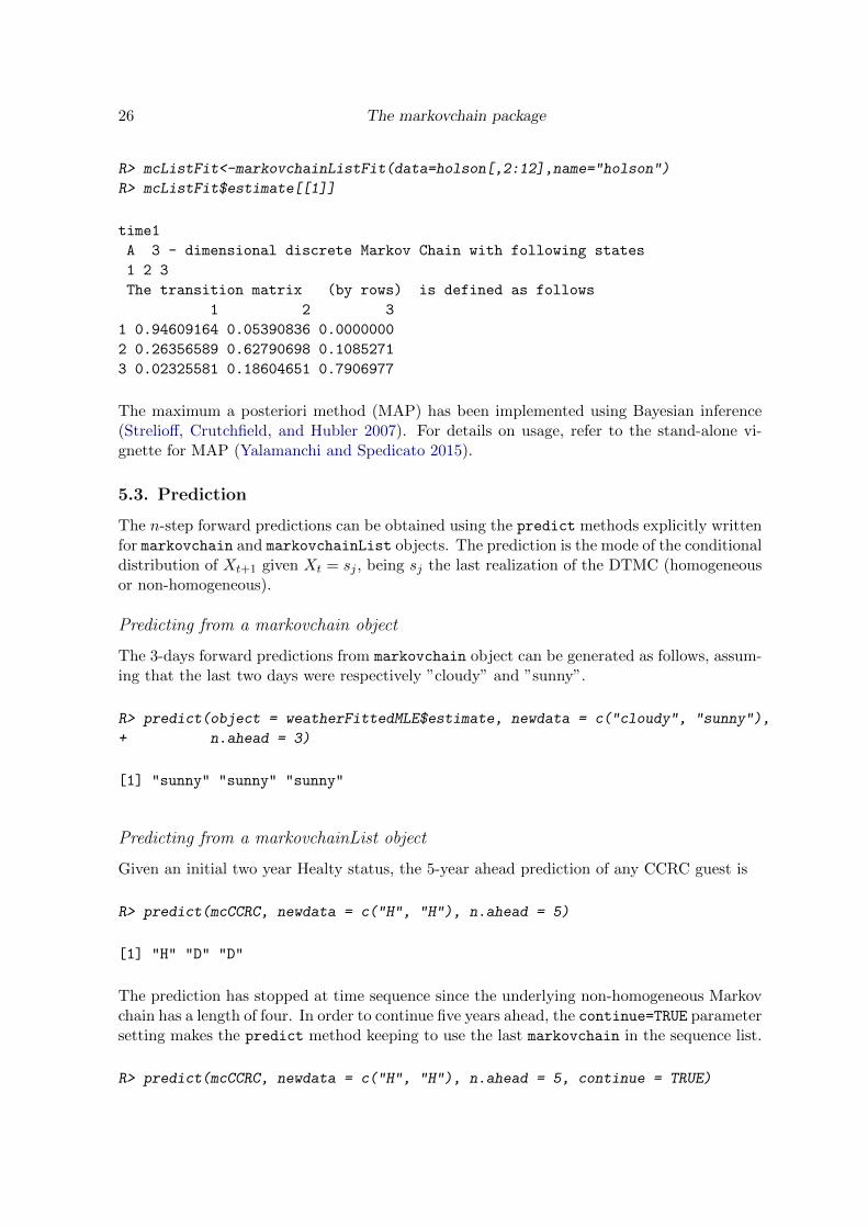
R> mcListFit<-markovchainListFit(data=holson[,2:12],name="holson")
R> mcListFit$estimate[[1]]
time1
A 3 - dimensional discrete Markov Chain with following states
1 2 3
The transition matrix (by rows) is defined as follows
1 2 3
1 0.94609164 0.05390836 0.0000000
2 0.26356589 0.62790698 0.1085271
3 0.02325581 0.18604651 0.7906977
The maximum a posteriori method (MAP) has been implemented using Bayesian inference(Strelioff, Crutchfield, and Hubler 2007). For details on usage, refer to the stand-alone vi-gnette for MAP (Yalamanchi and Spedicato 2015).
5.3. Prediction
The n-step forward predictions can be obtained using the predict methods explicitly writtenfor markovchain and markovchainList objects. The prediction is the mode of the conditionaldistribution of Xt+1 given Xt = sj , being sj the last realization of the DTMC (homogeneousor non-homogeneous).
Predicting from a markovchain object
The 3-days forward predictions from markovchain object can be generated as follows, assum-ing that the last two days were respectively ”cloudy” and ”sunny”.
R> predict(object = weatherFittedMLE$estimate, newdata = c("cloudy", "sunny"),
+ n.ahead = 3)
[1] "sunny" "sunny" "sunny"
Predicting from a markovchainList object
Given an initial two year Healty status, the 5-year ahead prediction of any CCRC guest is
R> predict(mcCCRC, newdata = c("H", "H"), n.ahead = 5)
[1] "H" "D" "D"
The prediction has stopped at time sequence since the underlying non-homogeneous Markovchain has a length of four. In order to continue five years ahead, the continue=TRUE parametersetting makes the predict method keeping to use the last markovchain in the sequence list.
R> predict(mcCCRC, newdata = c("H", "H"), n.ahead = 5, continue = TRUE)
Giorgio Alfredo Spedicato, Tae Seung Kang, Sai Bhargav Yalamanchi 27
[1] "H" "D" "D" "D" "D"
6. Applications
This section shows applications of DTMC in various fields.
6.1. Weather forecasting
Markov chains provide a simple model to predict the next day’s weather given the currentmeteorological condition. The first application herewith shown is the ”Land of Oz example”from J. G. Kemeny, J. L.Snell, and G. L. Thompson (1974), the second is the ”Alofi IslandRainfall” from P. J. Avery and D. A. Henderson (1999).
Land of Oz
The Land of Oz is acknowledged not to have ideal weather conditions at all: the weather issnowy or rainy very often and, once more, there are never two nice days in a row. Considerthree weather states: rainy, nice and snowy. Let the transition matrix be as in the following:
R> mcWP <- new("markovchain", states = c("rainy", "nice", "snowy"),
+ transitionMatrix = matrix(c(0.5, 0.25, 0.25,
+ 0.5, 0, 0.5,
+ 0.25,0.25,0.5), byrow = T, nrow = 3))
Given that today it is a nice day, the corresponding stochastic row vector is w0 = (0 , 1 , 0)and the forecast after 1, 2 and 3 days are given by
R> W0 <- t(as.matrix(c(0, 1, 0)))
R> W1 <- W0 * mcWP; W1
rainy nice snowy
[1,] 0.5 0 0.5
R> W2 <- W0 * (mcWP ^ 2); W2
rainy nice snowy
[1,] 0.375 0.25 0.375
R> W3 <- W0 * (mcWP ^ 3); W3
rainy nice snowy
[1,] 0.40625 0.1875 0.40625
As can be seen from w1, if in the Land of Oz today is a nice day, tomorrow it will rain orsnow with probability 1. One week later, the prediction can be computed as
28 The markovchain package
R> W7 <- W0 * (mcWP ^ 7)
R> W7
rainy nice snowy
[1,] 0.4000244 0.1999512 0.4000244
The steady state of the chain can be computed by means of the steadyStates method.
R> q <- steadyStates(mcWP)
R> q
rainy nice snowy
[1,] 0.4 0.2 0.4
Note that, from the seventh day on, the predicted probabilities are substantially equal to thesteady state of the chain and they don’t depend from the starting point, as the following codeshows.
R> R0 <- t(as.matrix(c(1, 0, 0)))
R> R7 <- R0 * (mcWP ^ 7); R7
rainy nice snowy
[1,] 0.4000244 0.2000122 0.3999634
R> S0 <- t(as.matrix(c(0, 0, 1)))
R> S7 <- S0 * (mcWP ^ 7); S7
rainy nice snowy
[1,] 0.3999634 0.2000122 0.4000244
Alofi Island Rainfall
Alofi Island daily rainfall data were recorded from January 1st, 1987 until December 31st,1989 and classified into three states: ”0” (no rain), ”1-5” (from non zero until 5 mm) and ”6+”(more than 5mm). The corresponding dataset is provided within the markovchain package.
R> data("rain", package = "markovchain")
R> table(rain$rain)
0 1-5 6+
548 295 253
The underlying transition matrix is estimated as follows.
R> mcAlofi <- markovchainFit(data = rain$rain, name = "Alofi MC")$estimate
R> mcAlofi

Giorgio Alfredo Spedicato, Tae Seung Kang, Sai Bhargav Yalamanchi 29
Alofi MC
A 3 - dimensional discrete Markov Chain with following states
0 1-5 6+
The transition matrix (by rows) is defined as follows
0 1-5 6+
0 0.6605839 0.2299270 0.1094891
1-5 0.4625850 0.3061224 0.2312925
6+ 0.1976285 0.3122530 0.4901186
The long term daily rainfall distribution is obtained by means of the steadyStates method.
R> steadyStates(mcAlofi)
0 1-5 6+
[1,] 0.5008871 0.2693656 0.2297473
6.2. Finance and Economics
Other relevant applications of DTMC can be found in Finance and Economics.
Finance
Credit ratings transitions have been successfully modelled with discrete time Markov chains.Some rating agencies publish transition matrices that show the empirical transition proba-bilities across credit ratings. The example that follows comes from CreditMetrics R package(Wittmann 2007), carrying Standard & Poor’s published data.
R> rc <- c("AAA", "AA", "A", "BBB", "BB", "B", "CCC", "D")
R> creditMatrix <- matrix(c(90.81, 8.33, 0.68, 0.06, 0.08, 0.02, 0.01, 0.01,
+ 0.70, 90.65, 7.79, 0.64, 0.06, 0.13, 0.02, 0.01,
+ 0.09, 2.27, 91.05, 5.52, 0.74, 0.26, 0.01, 0.06,
+ 0.02, 0.33, 5.95, 85.93, 5.30, 1.17, 1.12, 0.18,
+ 0.03, 0.14, 0.67, 7.73, 80.53, 8.84, 1.00, 1.06,
+ 0.01, 0.11, 0.24, 0.43, 6.48, 83.46, 4.07, 5.20,
+ 0.21, 0, 0.22, 1.30, 2.38, 11.24, 64.86, 19.79,
+ 0, 0, 0, 0, 0, 0, 0, 100
+ )/100, 8, 8, dimnames = list(rc, rc), byrow = TRUE)
It is easy to convert such matrices into markovchain objects and to perform some analyses
R> creditMc <- new("markovchain", transitionMatrix = creditMatrix,
+ name = "S&P Matrix")
R> absorbingStates(creditMc)
[1] "D"

30 The markovchain package
Economics
For a recent application of markovchain in Economic, see Jacob (2014).
A dynamic system generates two kinds of economic effects (Bard 2000):
1. those incurred when the system is in a specified state, and
2. those incurred when the system makes a transition from one state to another.
Let the monetary amount of being in a particular state be represented as a m-dimensionalcolumn vector cS, while let the monetary amount of a transition be embodied in a CR matrixin which each component specifies the monetary amount of going from state i to state j in asingle step. Henceforth, Equation 15 represents the monetary of being in state i.
ci = cSi +m∑j=1
CRijpij . (15)
Let c = [ci] and let ei be the vector valued 1 in the initial state and 0 in all other, then, if fn isthe random variable representing the economic return associated with the stochastic processat time n, Equation 16 holds:
E [fn (Xn) |X0 = i] = eiPnc. (16)
The following example assumes that a telephone company models the transition probabilitiesbetween customer/non-customer status by matrix P and the cost associated to states bymatrix M .
R> statesNames <- c("customer", "non customer")
R> P <- zeros(2); P[1, 1] <- .9; P[1, 2] <- .1; P[2, 2] <- .95; P[2, 1] <- .05;
R> rownames(P) <- statesNames; colnames(P) <- statesNames
R> mcP <- new("markovchain", transitionMatrix = P, name = "Telephone company")
R> M <- zeros(2); M[1, 1] <- -20; M[1, 2] <- -30; M[2, 1] <- -40; M[2, 2] <- 0
If the average revenue for existing customer is +100, the cost per state is computed as follows.
R> c1 <- 100 + conditionalDistribution(mcP, state = "customer") %*% M[1,]
R> c2 <- 0 + conditionalDistribution(mcP, state = "non customer") %*% M[2,]
For an existing customer, the expected gain (loss) at the fifth year is given by the followingcode.
R> as.numeric((c(1, 0)* mcP ^ 5) %*% (as.vector(c(c1, c2))))
[1] 48.96009
Giorgio Alfredo Spedicato, Tae Seung Kang, Sai Bhargav Yalamanchi 31
6.3. Actuarial science
Markov chains are widely applied in the field of actuarial science. Two classical applicationsare policyholders’ distribution across Bonus Malus classes in Motor Third Party Liability(MTPL) insurance (Section 6.3.1) and health insurance pricing and reserving (Section 6.3.2).
MPTL Bonus Malus
Bonus Malus (BM) contracts grant the policyholder a discount (enworsen) as a function ofthe number of claims in the experience period. The discount (enworsen) is applied on a pre-mium that already allows for known (a priori) policyholder characteristics (Denuit, Marechal,Pitrebois, and Walhin 2007) and it usually depends on vehicle, territory, the demographicprofile of the policyholder, and policy coverages deep (deductible and policy limits).Since the proposed BM level depends on the claim on the previous period, it can be modelledby a discrete Markov chain. A very simplified example follows. Assume a BM scale from 1to 5, where 4 is the starting level. The evolution rules are shown in Equation 17:
bmt+1 = max (1, bmt − 1) ∗(N = 0
)+ min
(5, bmt + 2 ∗ N
)∗(N ≥ 1
). (17)
Tthe number of claim N is a random variable that is assumed to be Poisson distributed.
R> getBonusMalusMarkovChain <- function(lambda)
+ {
+ bmMatr <- zeros(5)
+ bmMatr[1, 1] <- dpois(x = 0, lambda)
+ bmMatr[1, 3] <- dpois(x = 1, lambda)
+ bmMatr[1, 5] <- 1 - ppois(q = 1, lambda)
+
+ bmMatr[2, 1] <- dpois(x = 0, lambda)
+ bmMatr[2, 4] <- dpois(x = 1, lambda)
+ bmMatr[2, 5] <- 1 - ppois(q = 1, lambda)
+
+ bmMatr[3, 2] <- dpois(x = 0, lambda)
+ bmMatr[3, 5] <- 1 - dpois(x=0, lambda)
+
+ bmMatr[4, 3] <- dpois(x = 0, lambda)
+ bmMatr[4, 5] <- 1 - dpois(x = 0, lambda)
+
+ bmMatr[5, 4] <- dpois(x = 0, lambda)
+ bmMatr[5, 5] <- 1 - dpois(x = 0, lambda)
+ stateNames <- as.character(1:5)
+ out <- new("markovchain", transitionMatrix = bmMatr,
+ states = stateNames, name = "BM Matrix")
+ return(out)
+ }
R>
Assuming that the a-priori claim frequency per car-year is 0.05 in the class (being the class
32 The markovchain package
the group of policyholders that share the same common characteristics), the underlying BMtransition matrix and its underlying steady state are as follows.
R> bmMc <- getBonusMalusMarkovChain(0.05)
R> as.numeric(steadyStates(bmMc))
[1] 0.895836079 0.045930498 0.048285405 0.005969247 0.003978772
If the underlying BM coefficients of the class are 0.5, 0.7, 0.9, 1.0, 1.25, this means that theaverage BM coefficient applied on the long run to the class is given by
R> sum(as.numeric(steadyStates(bmMc)) * c(0.5, 0.7, 0.9, 1, 1.25))
[1] 0.534469
This means that the average premium paid by policyholders in the portfolio almost halves inthe long run.
Health insurance example
Actuaries quantify the risk inherent in insurance contracts evaluating the premium of insur-ance contract to be sold (therefore covering future risk) and evaluating the actuarial reservesof existing portfolios (the liabilities in terms of benefits or claims payments due to policy-holder arising from previously sold contracts). Key quantities of actuarial interest are: theexpected present value of future benefits, PV FB, the (periodic) benefit premium, P , andthe present value of future premium PV FP . A level benefit premium could be set equatingat the beginning of the contract PV FB = PV FP . After the beginning of the contract thebenefit reserve is the difference between PV FB and PV FP . The example comes from Desh-mukh (2012). The interest rate is 5%, benefits are payable upon death (1000) and disability(500). Premiums are payable at the beginning of period only if the policyholder is active.The contract term is three years.
R> mcHI <- new("markovchain", states = c("active", "disable", "withdrawn",
+ "death"),
+ transitionMatrix = matrix(c(0.5, .25, .15, .1,
+ 0.4, 0.4, 0.0, 0.2,
+ 0, 0, 1, 0,
+ 0, 0, 0, 1), byrow = TRUE, nrow = 4))
R> benefitVector <- as.matrix(c(0, 0, 500, 1000))
The policyholders is active at T0. Therefore the expected states at T1, . . . T3 are calculated inthe following.
R> T0 <- t(as.matrix(c(1, 0, 0, 0)))
R> T1 <- T0 * mcHI
R> T2 <- T1 * mcHI
R> T3 <- T2 * mcHI
Giorgio Alfredo Spedicato, Tae Seung Kang, Sai Bhargav Yalamanchi 33
The present value of future benefit at T0 is given by
R> PVFB <- T0 %*% benefitVector * 1.05 ^ -0 +
+ T1 %*% benefitVector * 1.05 ^ -1+
+ T2 %*% benefitVector * 1.05 ^ -2 + T3 %*% benefitVector * 1.05 ^ -3
The yearly premium payable whether the insured is alive is as follows.
R> P <- PVFB / (T0[1] * 1.05 ^- 0 + T1[1] * 1.05 ^ -1 + T2[1] * 1.05 ^ -2)
The reserve at the beginning of the second year, in the case of the insured being alive, is asfollows.
R> PVFB <- T2 %*% benefitVector * 1.05 ^ -1 + T3 %*% benefitVector * 1.05 ^ -2
R> PVFP <- P*(T1[1] * 1.05 ^ -0 + T2[1] * 1.05 ^ -1)
R> V <- PVFB - PVFP
R> V
[,1]
[1,] 300.2528
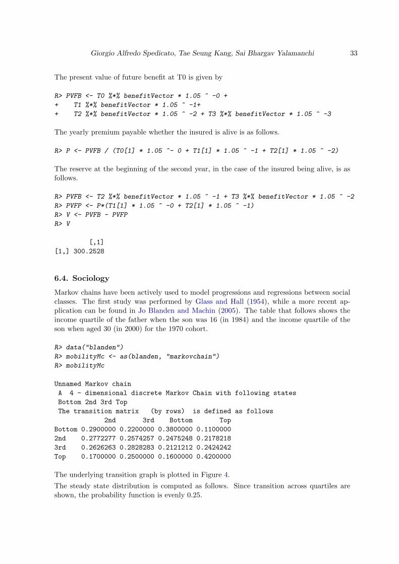
6.4. Sociology
Markov chains have been actively used to model progressions and regressions between socialclasses. The first study was performed by Glass and Hall (1954), while a more recent ap-plication can be found in Jo Blanden and Machin (2005). The table that follows shows theincome quartile of the father when the son was 16 (in 1984) and the income quartile of theson when aged 30 (in 2000) for the 1970 cohort.
R> data("blanden")
R> mobilityMc <- as(blanden, "markovchain")
R> mobilityMc
Unnamed Markov chain
A 4 - dimensional discrete Markov Chain with following states
Bottom 2nd 3rd Top
The transition matrix (by rows) is defined as follows
2nd 3rd Bottom Top
Bottom 0.2900000 0.2200000 0.3800000 0.1100000
2nd 0.2772277 0.2574257 0.2475248 0.2178218
3rd 0.2626263 0.2828283 0.2121212 0.2424242
Top 0.1700000 0.2500000 0.1600000 0.4200000
The underlying transition graph is plotted in Figure 4.
The steady state distribution is computed as follows. Since transition across quartiles areshown, the probability function is evenly 0.25.
34 The markovchain package
1970 mobility
0.29
0.26
0.21
0.420.28
0.26
0.17
0.22
0.28
0.25
0.38
0.25
0.16
0.11
0.22
0.242nd
3rd
Bottom
Top
Figure 4: 1970 UK cohort mobility data.

Giorgio Alfredo Spedicato, Tae Seung Kang, Sai Bhargav Yalamanchi 35
R> round(steadyStates(mobilityMc), 2)
Bottom 2nd 3rd Top
[1,] 0.25 0.25 0.25 0.25
6.5. Genetics and Medicine
This section contains two examples: the first shows the use of Markov chain models in genetics,the second shows an application of Markov chains in modelling diseases’ dynamics.
Genetics
P. J. Avery and D. A. Henderson (1999) discusses the use of Markov chains in model Preprogu-cacon gene protein bases sequence. The preproglucacon dataset in markovchain containsthe dataset shown in the package.
R> data("preproglucacon", package = "markovchain")
It is possible to model the transition probabilities between bases as shown in the followingcode.
R> mcProtein <- markovchainFit(preproglucacon$preproglucacon,
+ name = "Preproglucacon MC")$estimate
R> mcProtein
Preproglucacon MC
A 4 - dimensional discrete Markov Chain with following states
A C G T
The transition matrix (by rows) is defined as follows
A C G T
A 0.3585271 0.1434109 0.16666667 0.3313953
C 0.3840304 0.1558935 0.02281369 0.4372624
G 0.3053097 0.1991150 0.15044248 0.3451327
T 0.2844523 0.1819788 0.17667845 0.3568905
Medicine
Discrete-time Markov chains are also employed to study the progression of chronic diseases.The following example is taken from B. A. Craig and A. A. Sendi (2002). Starting from sixmonth follow-up data, the maximum likelihood estimation of the monthly transition matrix isobtained. This transition matrix aims to describe the monthly progression of CD4-cell countsof HIV infected subjects.
R> craigSendiMatr <- matrix(c(682, 33, 25,
+ 154, 64, 47,
+ 19, 19, 43), byrow = T, nrow = 3)

36 The markovchain package
R> hivStates <- c("0-49", "50-74", "75-UP")
R> rownames(craigSendiMatr) <- hivStates
R> colnames(craigSendiMatr) <- hivStates
R> craigSendiTable <- as.table(craigSendiMatr)
R> mcM6 <- as(craigSendiTable, "markovchain")
R> mcM6@name <- "Zero-Six month CD4 cells transition"
R> mcM6
Zero-Six month CD4 cells transition
A 3 - dimensional discrete Markov Chain with following states
0-49 50-74 75-UP
The transition matrix (by rows) is defined as follows
0-49 50-74 75-UP
0-49 0.9216216 0.04459459 0.03378378
50-74 0.5811321 0.24150943 0.17735849
75-UP 0.2345679 0.23456790 0.53086420
As shown in the paper, the second passage consists in the decomposition of M6 = V ·D ·V −1in order to obtain M1 as M1 = V ·D1/6 · V −1 .
R> eig <- eigen(mcM6@transitionMatrix)
R> D <- diag(eig$values)
R> V <- eig$vectors
R> V %*% D %*% solve(V)
[,1] [,2] [,3]
[1,] 0.9216216 0.04459459 0.03378378
[2,] 0.5811321 0.24150943 0.17735849
[3,] 0.2345679 0.23456790 0.53086420
R> d <- D ^ (1/6)
R> M <- V %*% d %*% solve(V)
R> mcM1 <- new("markovchain", transitionMatrix = M, states = hivStates)
7. Discussion, issues and future plans
The markovchain package has been designed in order to provide easily handling of DTMCand communication with alternative packages.
Some numerical issues have been found when working with matrix algebra using R internallinear algebra kernel (the same calculations performed with MATLAB gave a more accurateresult). Some temporary workarounds have been implemented. For example, the conditionfor row/column sums to be equal to one is valid up to fifth decimal. Similarly, when extractingthe eigenvectors only the real part is taken.

Giorgio Alfredo Spedicato, Tae Seung Kang, Sai Bhargav Yalamanchi 37
Such limitations are expected to be overcome in future releases. Similarly, future versions ofthe package are expected to improve the code in terms of numerical accuracy and rapidity.An intitial rewriting of internal function in C++ by means of Rcpp package (Eddelbuettel2013) has been started.
Aknowledgments
The author wishes to thank Michael Cole, Tobi Gutman and Mildenberger Thoralf for theirsuggestions and bug checks. A very special thanks also to Tae Seung Kang (and to the otherGoogle Summer of Code 2015 candidates) for having rewritten the fitting functions into Rcpp.A final thanks also to Dr. Simona C. Minotti and Dr. Mirko Signorelli for their support indrafting this version of the vignettes.
References
B A Craig, A A Sendi (2002). “Estimation of the Transition Matrix of a Discrete-TimeMarkov Chain.” Health Economics, 11, 33–42.
Bard JF (2000). “Lecture 12.5 - Additional Issues Concerning Discrete-TimeMarkov Chains.” URL http://www.me.utexas.edu/~jensen%20/ORMM/instruction/
powerpoint/or_models_09/12.5_dtmc2.ppt.
Bremaud P (1999). “Discrete-Time Markov Models.” In Markov Chains, pp. 53–93. Springer.
Chambers J (2008). Software for Data Analysis: Programming with R. Statistics and com-puting. Springer-Verlag. ISBN 9780387759357.
Ching W, Ng M (2006). Markov Chains: Models, Algorithms and Applications. Inter-national Series in Operations Research & Management Science. Springer-Verlag. ISBN9780387293356.
Csardi G, Nepusz T (2006). “The igraph Software Package for Complex Network Research.”InterJournal, Complex Systems, 1695. URL http://igraph.sf.net.
de Wreede LC, Fiocco M, Putter H (2011). “mstate: An R Package for the Analysis ofCompeting Risks and Multi-State Models.” Journal of Statistical Software, 38(7), 1–30.URL http://www.jstatsoft.org/v38/i07/.
Denuit M, Marechal X, Pitrebois S, Walhin JF (2007). Actuarial modelling of claim counts:Risk classification, credibility and bonus-malus systems. Wiley.
Deshmukh S (2012). Multiple Decrement Models in Insurance: An Introduction Using R.SpringerLink : Bucher. Springer-Verlag. ISBN 9788132206590.
Eddelbuettel D (2013). Seamless R and C++ Integration with Rcpp. Springer-Verlag, NewYork. ISBN 978-1-4614-6867-7.
Feres R (2007). “Notes for Math 450 MATLAB Listings for Markov Chains.” URL http:
//www.math.wustl.edu/~feres/Math450Lect04.pdf.
38 The markovchain package
Geyer CJ, Johnson LT (2013). mcmc: Markov Chain Monte Carlo. R package version 0.9-2,URL http://CRAN.R-project.org/package=mcmc.
Glass D, Hall JR (1954). “Social Mobility in Great Britain: A Study in IntergenerationalChange in Status.” In Social Mobility in Great Britain. Routledge and Kegan Paul.
Goulet V, Dutang C, Maechler M, Firth D, Shapira M, Stadelmann M, expm-developers@listsR-forgeR-projectorg (2013). expm: Matrix Exponential. R package version0.99-1, URL http://CRAN.R-project.org/package=expm.
Himmelmann SSDDL, wwwlinhicom (2010). HMM: HMM - Hidden Markov Models. Rpackage version 1.0, URL http://CRAN.R-project.org/package=HMM.
J G Kemeny, J LSnell, G L Thompson (1974). Introduction to Finite Mathematics. PrenticeHall.
Jackson CH (2011). “Multi-State Models for Panel Data: The msm Package for R.” Journalof Statistical Software, 38(8), 1–29. URL http://www.jstatsoft.org/v38/i08/.
Jacob I (2014). “Is R Cost Effective?” Electronic. Presented on Manchester R Meet-ing, URL http://www.rmanchester.org/Presentations/Ian%20Jacob%20-%20Is%20R%
20Cost%20Effective.pdf.
Jo Blanden PG, Machin S (2005). “Intergenerational Mobility in Europe and North America.”Technical report, Center for Economic Performances. URL http://cep.lse.ac.uk/about/
news/IntergenerationalMobility.pdf.
Montgomery J (2009). “Communication Classes.” URL http://www.ssc.wisc.edu/
~jmontgom/commclasses.pdf.
Nicholson W (2013). DTMCPack: Suite of Functions Related to Discrete-Time Discrete-State Markov Chains. R package version 0.1-2, URL http://CRAN.R-project.org/
package=DTMCPack.
P J Avery, D A Henderson (1999). “Fitting Markov Chain Models to Discrete State Series.”Applied Statistics, 48(1), 53–61.
R Core Team (2013). R: A Language and Environment for Statistical Computing. R Foun-dation for Statistical Computing, Vienna, Austria. URL http://www.R-project.org/.
Roebuck P (2011). matlab: MATLAB emulation package. R package version 0.8.9, URLhttp://CRAN.R-project.org/package=matlab.
Snell L (1999). “Probability Book: chapter 11.” URL http://www.dartmouth.edu/~chance/
teaching_aids/books_articles/probability_book/Chapter11.pdf.
Spedicato GA (2015). markovchain: an R Package to Easily Handle Discrete MarkovChains. R package version 0.2.2.
Strelioff CC, Crutchfield JP, Hubler AW (2007). “Inferring Markov Chains: Bayesian Esti-mation, Model Comparison, Entropy Rate, and Out-of-class Modeling.” Sante Fe WorkingPapers. URL http://arxiv.org/abs/math/0703715/.
Giorgio Alfredo Spedicato, Tae Seung Kang, Sai Bhargav Yalamanchi 39
Wittmann A (2007). CreditMetrics: Functions for Calculating the CreditMetrics Risk Model.R package version 0.0-2.
Wolfram Research I (2013a). URL http://www.wolfram.com/mathematica/new-in-9/
markov-chains-and-queues/structural-properties-of-finite-markov-processes.
html.
Wolfram Research I (2013b). Mathematica. Wolfram Research, Inc., ninth edition.
Yalamanchi SB, Spedicato GA (2015). Bayesian Inference of First Order Markov Chains. Rpackage version 0.2.5.
Affiliation:
Giorgio Alfredo SpedicatoPh.D C.Stat ACASUnipolSai R&DVia Firenze 11, Paderno Dugnano 20037 ItalyTelephone: +39/334/6634384E-mail: [email protected]: www.statisticaladvisor.com
Tae Seung KangPh.D studentComputer & Information Science & EngineeringUniversity of FloridaGainesville, FL, USAE-mail: [email protected]
Sai Bhargav YalamanchiB-Tech studentElectrical EngineeringIndian Institute of Technology, BombayMumbai - 400 076, IndiaE-mail: [email protected]