the markovchain package: a package for easily handling discrete
TRANSCRIPT
The markovchain Package: A Package for Easily
Handling Discrete Markov Chains in R
Giorgio Alfredo Spedicato, Tae Seung Kang, Sai Bhargav Yalamanchi and Deepak Yadav
Abstract
The markovchain package aims to fill a gap within the R framework providing S4classes and methods for easily handling discrete time Markov chains, homogeneous andsimple inhomogeneous ones as well as continuous time Markov chains. The S4 classesfor handling and analysing discrete and continuous time Markov chains are presented, aswell as functions and method for performing probabilistic and statistical analysis. Finally,some examples in which the package’s functions are applied to Economics, Finance andNatural Sciences topics are shown.
Keywords: discrete time Markov chains, continuous time Markov chains, transition matrices,communicating classes, periodicity, first passage time, stationary distributions..
1. Introduction
Markov chains represent a class of stochastic processes of great interest for the wide spectrumof practical applications. In particular, discrete time Markov chains (DTMC) permit to modelthe transition probabilities between discrete states by the aid of matrices. Various R packagesdeal with models that are based on Markov chains:
� msm (Jackson 2011) handles Multi-State Models for panel data;
� mcmcR (Geyer and Johnson 2013) implements Monte Carlo Markov Chain approach;
� hmm (Himmelmann and www.linhi.com 2010) fits hidden Markov models with covari-ates;
� mstate fits Multi-State Models based on Markov chains for survival analysis (de Wreede,Fiocco, and Putter 2011).
Nevertheless, the R statistical environment (R Core Team 2013) seems to lack a simple packagethat coherently defines S4 classes for discrete Markov chains and allows to perform probabilis-tic analysis, statistical inference and applications. For the sake of completeness, markovchainis the second package specifically dedicated to DTMC analysis, being DTMCPack (Nicholson2013) the first one. Notwithstanding, markovchain package (Spedicato 2017) aims to offermore flexibility in handling DTMC than other existing solutions, providing S4 classes for bothhomogeneous and non-homogeneous Markov chains as well as methods suited to perform sta-tistical and probabilistic analysis.The markovchain package depends on the following R packages: expm (Goulet, Dutang,
2 The markovchain package
Maechler, Firth, Shapira, Stadelmann, and [email protected] 2013)to perform efficient matrices powers; igraph (Csardi and Nepusz 2006) to perform pretty plot-ting of markovchain objects and matlab (Roebuck 2011), that contains functions for matrixmanagement and calculations that emulate those within MATLAB environment. Moreover,other scientific softwares provide functions specifically designed to analyze DTMC, as Math-ematica 9 (Wolfram Research 2013b).The paper is structured as follows: Section 2 briefly reviews mathematics and definitions re-garding DTMC, Section 3 discusses how to handle and manage Markov chain objects withinthe package, Section 4 and Section 5 show how to perform probabilistic and statistical mod-elling, while Section 6 presents some applied examples from various fields analyzed by meansof the markovchain package.
2. Review of core mathematical concepts
2.1. General Definitions
A DTMC is a sequence of random variables X1, X2 , . . . , Xn, . . . characterized by the Markovproperty (also known as memoryless property, see Equation 1). The Markov property statesthat the distribution of the forthcoming state Xn+1 depends only on the current state Xn
and doesn’t depend on the previous ones Xn−1, Xn−2, . . . , X1.
Pr (Xn+1 = xn+1 |X1 = x1, X2 = x2,..., Xn = xn ) = Pr (Xn+1 = xn+1 |Xn = xn ) . (1)
The set of possible states S = {s1, s2, ..., sr} of Xn can be finite or countable and it is namedthe state space of the chain.
The chain moves from one state to another (this change is named either ’transition’ or ’step’)and the probability pij to move from state si to state sj in one step is named transitionprobability:
pij = Pr (X1 = sj |X0 = si ) . (2)
The probability of moving from state i to j in n steps is denoted by p(n)ij = Pr (Xn = sj |X0 = si ).
A DTMC is called time-homogeneous if the property shown in Equation 3 holds. Timehomogeneity implies no change in the underlying transition probabilities as time goes on.
Pr (Xn+1 = sj |Xn = si ) = Pr (Xn = sj |Xn−1 = si ) . (3)
If the Markov chain is time-homogeneous, then pij = Pr (Xk+1 = sj |Xk = si ) and
p(n)ij = Pr (Xn+k = sj |Xk = si ), where k > 0.
The probability distribution of transitions from one state to another can be represented intoa transition matrix P = (pij)i,j , where each element of position (i, j) represents the transitionprobability pij . E.g., if r = 3 the transition matrix P is shown in Equation 4
P =
p11 p12 p13p21 p22 p23p31 p32 p33
. (4)
Giorgio Alfredo Spedicato, Tae Seung Kang, Sai Bhargav Yalamanchi, Deepak Yadav 3
The distribution over the states can be written in the form of a stochastic row vector x (theterm stochastic means that
∑i xi = 1, xi ≥ 0): e.g., if the current state of x is s2, x = (0 1 0).
As a consequence, the relation between x(1) and x(0) is x(1) = x(0)P and, recursively, we getx(2) = x(0)P 2 and x(n) = x(0)Pn, n > 0.
DTMC are explained in most theory books on stochastic processes, see Bremaud (1999) andDobrow (2016) for example. Valuable references online available are: Konstantopoulos (2009),Snell (1999) and Bard (2000).
2.2. Properties and classification of states
A state sj is said accessible from state si (written si → sj) if a system started in state si hasa positive probability to reach the state sj at a certain point, i.e., ∃n > 0 : pnij > 0. If bothsi → sj and sj → si, then si and sj are said to communicate.
A communicating class is defined to be a set of states that communicate. A DTMC can becomposed by one or more communicating classes. If the DTMC is composed by only onecommunicating class (i.e., if all states in the chain communicate), then it is said irreducible.A communicating class is said to be closed if no states outside of the class can be reachedfrom any state inside it.
If pii = 1, si is defined as absorbing state: an absorbing state corresponds to a closed com-municating class composed by one state only.
The canonic form of a DTMC transition matrix is a matrix having a block form, where theclosed communicating classes are shown at the beginning of the diagonal matrix.
A state si has period ki if any return to state si must occur in multiplies of ki steps, that iski = gcd {n : Pr (Xn = si |X0 = si ) > 0}, where gcd is the greatest common divisor. If ki = 1the state si is said to be aperiodic, else if ki > 1 the state si is periodic with period ki. Looselyspeaking, si is periodic if it can only return to itself after a fixed number of transitions ki > 1(or multiple of ki), else it is aperiodic.
If states si and sj belong to the same communicating class, then they have the same period ki.As a consequence, each of the states of an irreducible DTMC share the same periodicity. Thisperiodicity is also considered the DTMC periodicity. It is possible to classify states accordingto their periodicity. Let T x→x is the number of periods to go back to state x knowing thatthe chain starts in x.
� A state x is recurrent if P (T x→x < +∞) = 1 (equivalently P (T x→x = +∞) = 0). Inaddition:
1. A state x is null recurrent if in addition E(T x→x) = +∞.
2. A state x is positive recurrent if in addition E(T x→x) < +∞.
3. A state x is absorbing if in addition P (T x→x = 1) = 1.
� A state x is transient if P (T x→x < +∞) < 1 (equivalently P (T x→x = +∞) > 0).
It is possible to analyze the timing to reach a certain state. The first passage time from statesi to state sj is the number Tij of steps taken by the chain until it arrives for the first timeto state sj , given that X0 = si. The probability distribution of Tij is defined by Equation 5
hij(n) = Pr (Tij = n) = Pr (Xn = sj , Xn−1 6= sj , . . . , X1 6= sj |X0 = si) (5)
4 The markovchain package
and can be found recursively using Equation 6, given that hij(n) = pij .
hij(n) =
∑k∈S−{sj}
pikhkj(n−1). (6)
If in the definition of the first passage time we let si = sj , we obtain the first return timeTi = inf{n ≥ 1 : Xn = si|X0 = si}. A state si is said to be recurrent if it is visited infinitelyoften, i.e., Pr(Ti < +∞|X0 = si) = 1. On the opposite, si is called transient if there is apositive probability that the chain will never return to si, i.e., Pr(Ti = +∞|X0 = si) > 0.
Given a time homogeneous Markov chain with transition matrix P, a stationary distributionz is a stochastic row vector such that z = z · P , where 0 ≤ zj ≤ 1 ∀j and
∑j zj = 1.
If a DTMC {Xn} is irreducible and aperiodic, then it has a limit distribution and this distri-bution is stationary. As a consequence, if P is the k × k transition matrix of the chain andz = (z1, ..., zk) is the eigenvector of P such that
∑ki=1 zi = 1, then we get
limn→∞
Pn = Z, (7)
where Z is the matrix having all rows equal to z. The stationary distribution of {Xn} isrepresented by z.
2.3. A short example
Consider the following numerical example. Suppose we have a DTMC with a set of 3 possiblestates S = {s1, s2, s3}. Let the transition matrix be
P =
0.5 0.2 0.30.15 0.45 0.40.25 0.35 0.4
. (8)
In P , p11 = 0.5 is the probability that X1 = s1 given that we observed X0 = s1 is 0.5, and soon. It is easy to see that the chain is irreducible since all the states communicate (it is madeby one communicating class only).
Suppose that the current state of the chain is X0 = s2, i.e., x(0) = (010), then the probabilitydistribution of states after 1 and 2 steps can be computed as shown in Equations 9 and 10.
x(1) = (0 1 0)
0.5 0.2 0.30.15 0.45 0.40.25 0.35 0.4
= (0.15 0.45 0.4) . (9)
x(n) = x(n−1)P → (0.15 0.45 0.4)
0.5 0.2 0.30.15 0.45 0.40.25 0.35 0.4
= (0.2425 0.3725 0.385) . (10)
If, f.e., we are interested in the probability of reaching the state s3 in two steps, thenPr (X2 = s3 |X0 = s2 ) = 0.385.
Giorgio Alfredo Spedicato, Tae Seung Kang, Sai Bhargav Yalamanchi, Deepak Yadav 5
3. The structure of the package
3.1. Creating markovchain objects
The package is loaded within the R command line as follows:
R> library("markovchain")
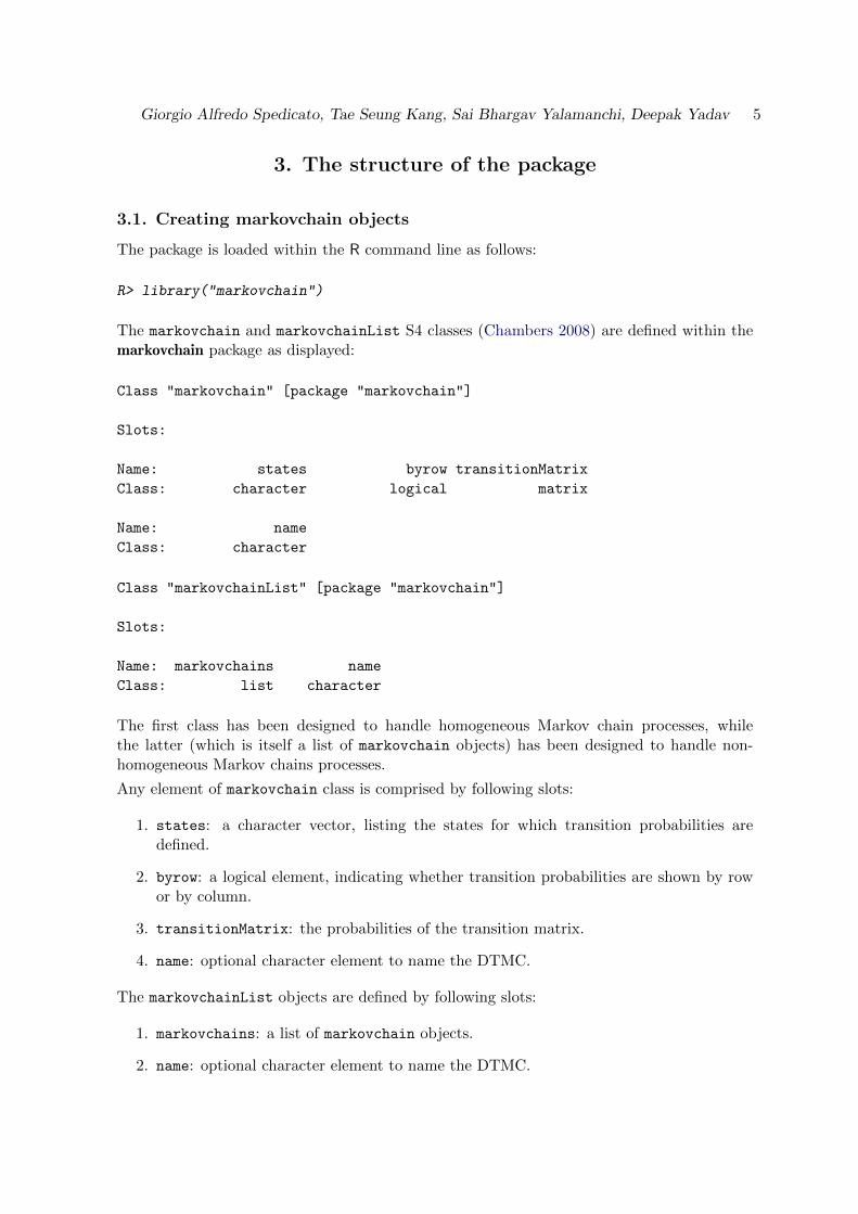
The markovchain and markovchainList S4 classes (Chambers 2008) are defined within themarkovchain package as displayed:
Class "markovchain" [package "markovchain"]
Slots:
Name: states byrow transitionMatrix
Class: character logical matrix
Name: name
Class: character
Class "markovchainList" [package "markovchain"]
Slots:
Name: markovchains name
Class: list character
The first class has been designed to handle homogeneous Markov chain processes, whilethe latter (which is itself a list of markovchain objects) has been designed to handle non-homogeneous Markov chains processes.
Any element of markovchain class is comprised by following slots:
1. states: a character vector, listing the states for which transition probabilities aredefined.
2. byrow: a logical element, indicating whether transition probabilities are shown by rowor by column.
3. transitionMatrix: the probabilities of the transition matrix.
4. name: optional character element to name the DTMC.
The markovchainList objects are defined by following slots:
1. markovchains: a list of markovchain objects.
2. name: optional character element to name the DTMC.
6 The markovchain package
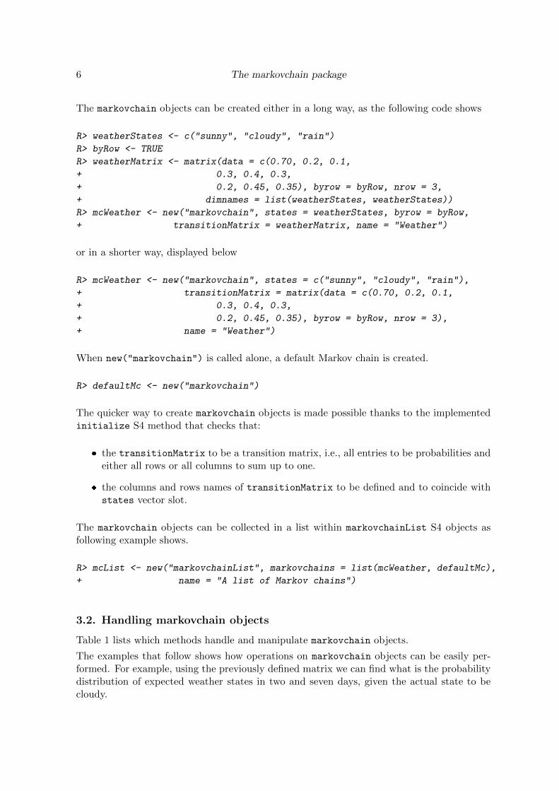
The markovchain objects can be created either in a long way, as the following code shows
R> weatherStates <- c("sunny", "cloudy", "rain")
R> byRow <- TRUE
R> weatherMatrix <- matrix(data = c(0.70, 0.2, 0.1,
+ 0.3, 0.4, 0.3,
+ 0.2, 0.45, 0.35), byrow = byRow, nrow = 3,
+ dimnames = list(weatherStates, weatherStates))
R> mcWeather <- new("markovchain", states = weatherStates, byrow = byRow,
+ transitionMatrix = weatherMatrix, name = "Weather")
or in a shorter way, displayed below
R> mcWeather <- new("markovchain", states = c("sunny", "cloudy", "rain"),
+ transitionMatrix = matrix(data = c(0.70, 0.2, 0.1,
+ 0.3, 0.4, 0.3,
+ 0.2, 0.45, 0.35), byrow = byRow, nrow = 3),
+ name = "Weather")
When new("markovchain") is called alone, a default Markov chain is created.
R> defaultMc <- new("markovchain")
The quicker way to create markovchain objects is made possible thanks to the implementedinitialize S4 method that checks that:
� the transitionMatrix to be a transition matrix, i.e., all entries to be probabilities andeither all rows or all columns to sum up to one.
� the columns and rows names of transitionMatrix to be defined and to coincide withstates vector slot.
The markovchain objects can be collected in a list within markovchainList S4 objects asfollowing example shows.
R> mcList <- new("markovchainList", markovchains = list(mcWeather, defaultMc),
+ name = "A list of Markov chains")
3.2. Handling markovchain objects
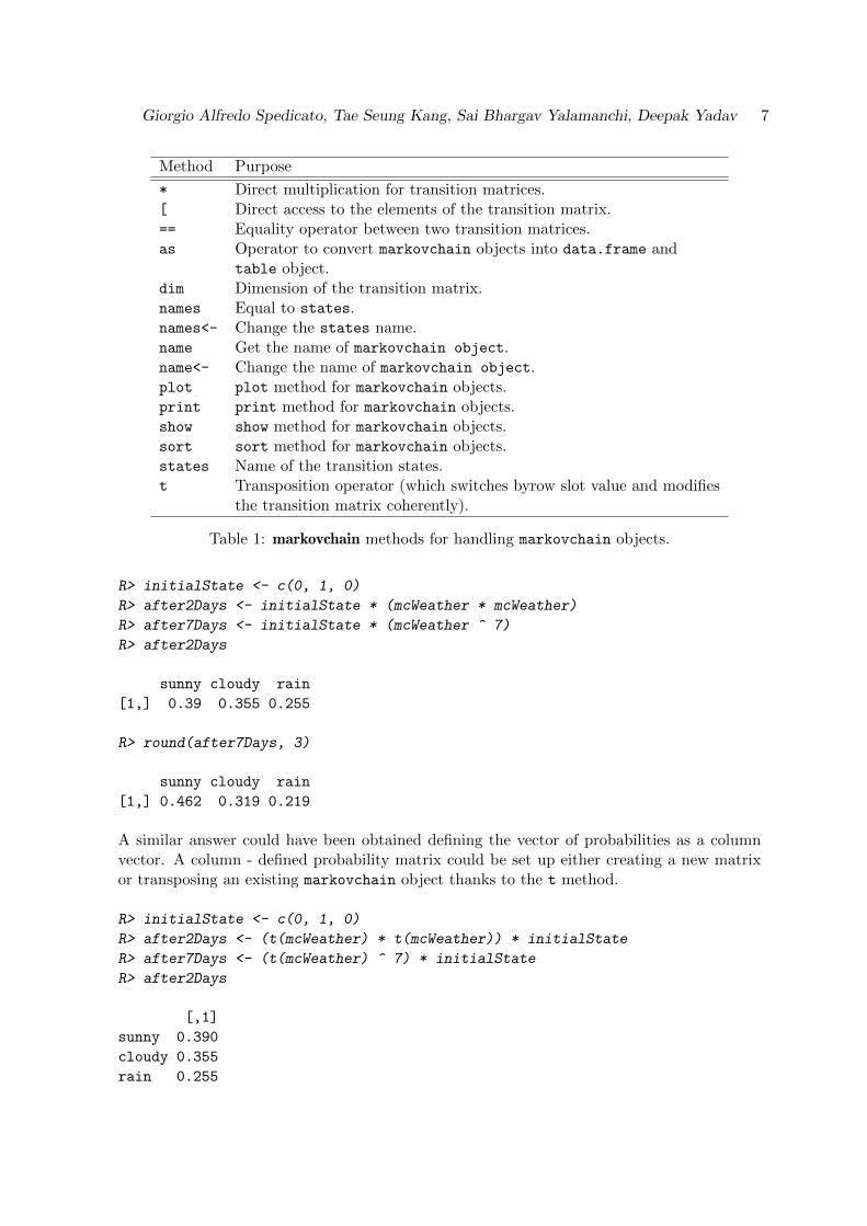
Table 1 lists which methods handle and manipulate markovchain objects.
The examples that follow shows how operations on markovchain objects can be easily per-formed. For example, using the previously defined matrix we can find what is the probabilitydistribution of expected weather states in two and seven days, given the actual state to becloudy.
Giorgio Alfredo Spedicato, Tae Seung Kang, Sai Bhargav Yalamanchi, Deepak Yadav 7
Method Purpose
* Direct multiplication for transition matrices.[ Direct access to the elements of the transition matrix.== Equality operator between two transition matrices.as Operator to convert markovchain objects into data.frame and
table object.dim Dimension of the transition matrix.names Equal to states.names<- Change the states name.name Get the name of markovchain object.name<- Change the name of markovchain object.plot plot method for markovchain objects.print print method for markovchain objects.show show method for markovchain objects.sort sort method for markovchain objects.states Name of the transition states.t Transposition operator (which switches byrow slot value and modifies
the transition matrix coherently).
Table 1: markovchain methods for handling markovchain objects.
R> initialState <- c(0, 1, 0)
R> after2Days <- initialState * (mcWeather * mcWeather)
R> after7Days <- initialState * (mcWeather ^ 7)
R> after2Days
sunny cloudy rain
[1,] 0.39 0.355 0.255
R> round(after7Days, 3)
sunny cloudy rain
[1,] 0.462 0.319 0.219
A similar answer could have been obtained defining the vector of probabilities as a columnvector. A column - defined probability matrix could be set up either creating a new matrixor transposing an existing markovchain object thanks to the t method.
R> initialState <- c(0, 1, 0)
R> after2Days <- (t(mcWeather) * t(mcWeather)) * initialState
R> after7Days <- (t(mcWeather) ^ 7) * initialState
R> after2Days
[,1]
sunny 0.390
cloudy 0.355
rain 0.255
8 The markovchain package
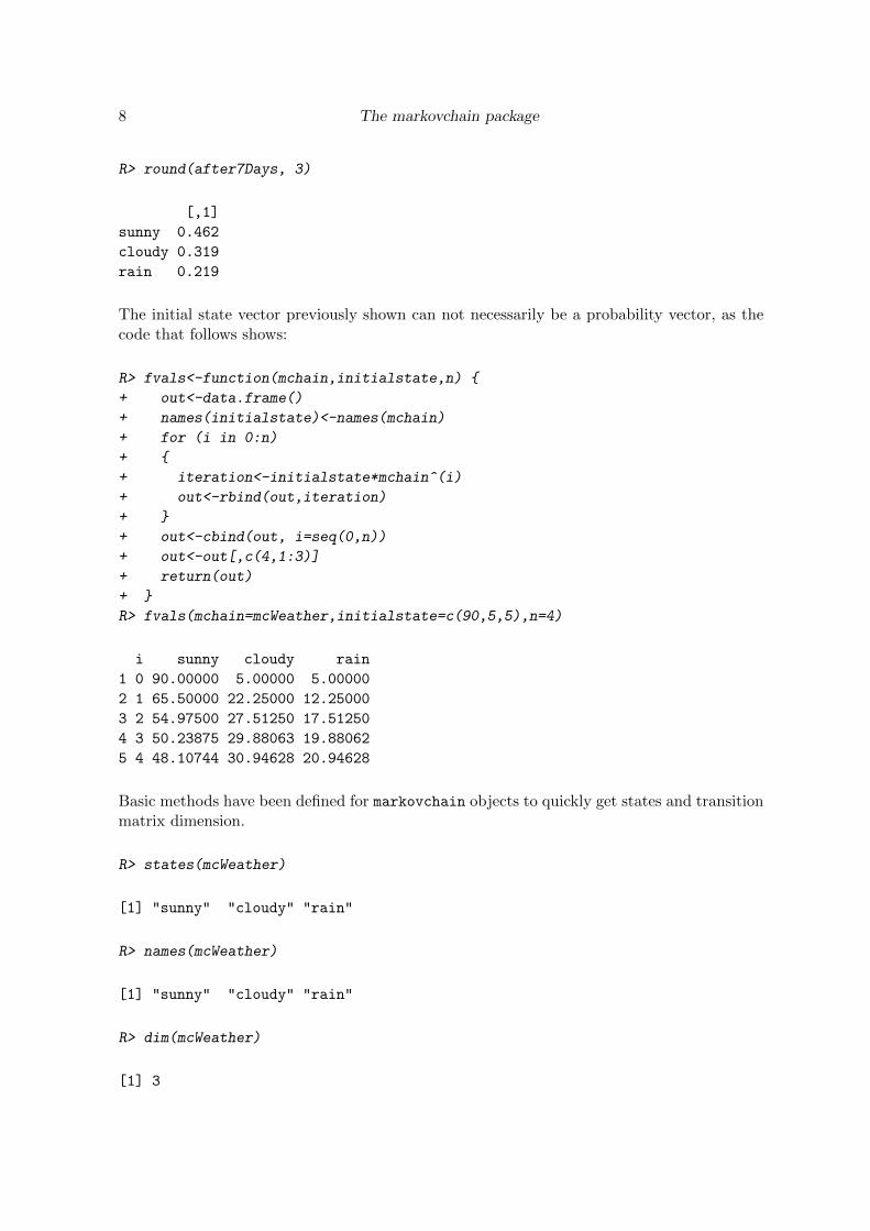
R> round(after7Days, 3)
[,1]
sunny 0.462
cloudy 0.319
rain 0.219
The initial state vector previously shown can not necessarily be a probability vector, as thecode that follows shows:
R> fvals<-function(mchain,initialstate,n) {
+ out<-data.frame()
+ names(initialstate)<-names(mchain)
+ for (i in 0:n)
+ {
+ iteration<-initialstate*mchain^(i)
+ out<-rbind(out,iteration)
+ }
+ out<-cbind(out, i=seq(0,n))
+ out<-out[,c(4,1:3)]
+ return(out)
+ }
R> fvals(mchain=mcWeather,initialstate=c(90,5,5),n=4)
i sunny cloudy rain
1 0 90.00000 5.00000 5.00000
2 1 65.50000 22.25000 12.25000
3 2 54.97500 27.51250 17.51250
4 3 50.23875 29.88063 19.88062
5 4 48.10744 30.94628 20.94628
Basic methods have been defined for markovchain objects to quickly get states and transitionmatrix dimension.
R> states(mcWeather)
[1] "sunny" "cloudy" "rain"
R> names(mcWeather)
[1] "sunny" "cloudy" "rain"
R> dim(mcWeather)
[1] 3
Giorgio Alfredo Spedicato, Tae Seung Kang, Sai Bhargav Yalamanchi, Deepak Yadav 9
Methods are available to set and get the name of markovchain object.
R> name(mcWeather)
[1] "Weather"
R> name(mcWeather) <- "New Name"
R> name(mcWeather)
[1] "New Name"
Also it is possible to alphabetically sort the transition matrix:
R> markovchain:::sort(mcWeather)
New Name
A 3 - dimensional discrete Markov Chain defined by the following states:
cloudy, rain, sunny
The transition matrix (by rows) is defined as follows:
cloudy rain sunny
cloudy 0.40 0.30 0.3
rain 0.45 0.35 0.2
sunny 0.20 0.10 0.7
A direct access to transition probabilities is provided both by transitionProbability methodand ”[” method.
R> transitionProbability(mcWeather, "cloudy", "rain")
[1] 0.3
R> mcWeather[2,3]
[1] 0.3
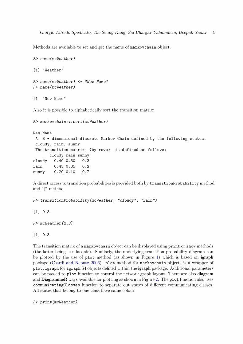
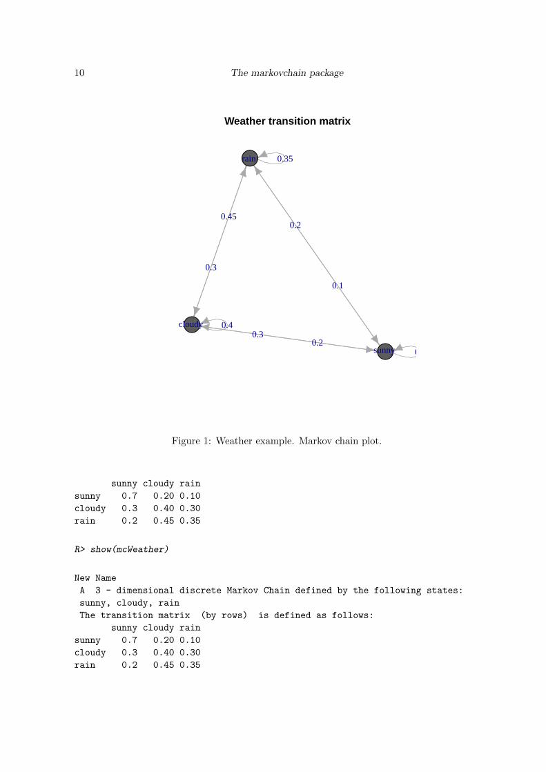
The transition matrix of a markovchain object can be displayed using print or show methods(the latter being less laconic). Similarly, the underlying transition probability diagram canbe plotted by the use of plot method (as shown in Figure 1) which is based on igraphpackage (Csardi and Nepusz 2006). plot method for markovchain objects is a wrapper ofplot.igraph for igraph S4 objects defined within the igraph package. Additional parameterscan be passed to plot function to control the network graph layout. There are also diagramand DiagrammeR ways available for plotting as shown in Figure 2. The plot function also usescommunicatingClasses function to separate out states of different communicating classes.All states that belong to one class have same colour.
R> print(mcWeather)
10 The markovchain package
Weather transition matrix
0.7
0.4
0.35
0.2
0.1
0.3
0.3
0.20.45
●
●
●
sunny
cloudy
rain
Figure 1: Weather example. Markov chain plot.
sunny cloudy rain
sunny 0.7 0.20 0.10
cloudy 0.3 0.40 0.30
rain 0.2 0.45 0.35
R> show(mcWeather)
New Name
A 3 - dimensional discrete Markov Chain defined by the following states:
sunny, cloudy, rain
The transition matrix (by rows) is defined as follows:
sunny cloudy rain
sunny 0.7 0.20 0.10
cloudy 0.3 0.40 0.30
rain 0.2 0.45 0.35
Giorgio Alfredo Spedicato, Tae Seung Kang, Sai Bhargav Yalamanchi, Deepak Yadav 11
0.70.2
0.1
0.3
0.4
0.30.20.45
0.35
sunnycloudy
rain
Figure 2: Weather example. Markov chain plot with diagram. plot(mcWeather, pack-age=”diagram”, box.size = 0.04)
12 The markovchain package
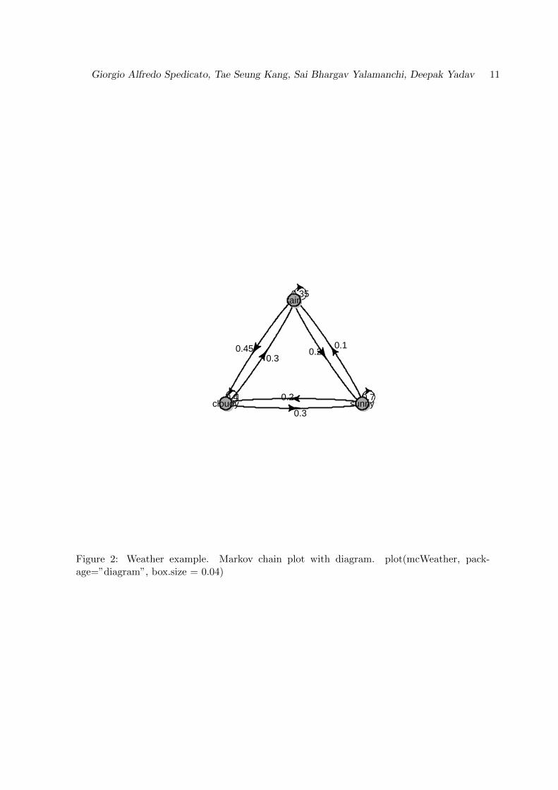
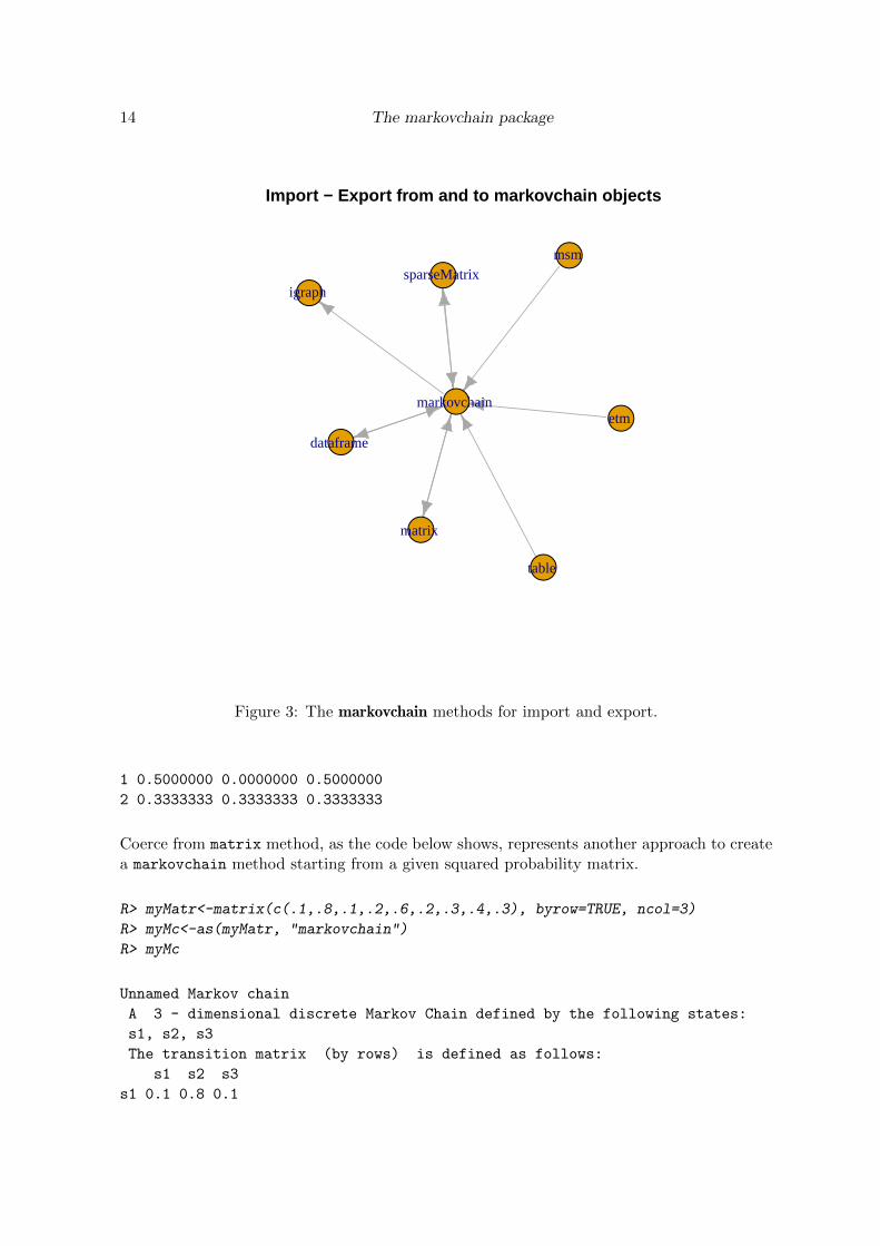
Import and export from some specific classes is possible, as shown in Figure 3 and in thefollowing code.
R> mcDf <- as(mcWeather, "data.frame")
R> mcNew <- as(mcDf, "markovchain")
R> mcDf
t0 t1 prob
1 sunny sunny 0.70
2 sunny cloudy 0.20
3 sunny rain 0.10
4 cloudy sunny 0.30
5 cloudy cloudy 0.40
6 cloudy rain 0.30
7 rain sunny 0.20
8 rain cloudy 0.45
9 rain rain 0.35
R> mcIgraph <- as(mcWeather, "igraph")
R> require(msm)
R> Q <- rbind ( c(0, 0.25, 0, 0.25),
+ c(0.166, 0, 0.166, 0.166),
+ c(0, 0.25, 0, 0.25),
+ c(0, 0, 0, 0) )
R> cavmsm <- msm(state ~ years, subject = PTNUM, data = cav, qmatrix = Q, death = 4)
R> msmMc <- as(cavmsm, "markovchain")
R> msmMc
Unnamed Markov chain
A 4 - dimensional discrete Markov Chain defined by the following states:
State 1, State 2, State 3, State 4
The transition matrix (by rows) is defined as follows:
State 1 State 2 State 3 State 4
State 1 0.853958721 0.08836953 0.01475543 0.04291632
State 2 0.155576908 0.56663284 0.20599563 0.07179462
State 3 0.009903994 0.07853691 0.65965727 0.25190183
State 4 0.000000000 0.00000000 0.00000000 1.00000000
R> library(etm)
R> data(sir.cont)
R> sir.cont <- sir.cont[order(sir.cont$id, sir.cont$time), ]
R> for (i in 2:nrow(sir.cont)) {
+ if (sir.cont$id[i]==sir.cont$id[i-1]) {
+ if (sir.cont$time[i]==sir.cont$time[i-1]) {
Giorgio Alfredo Spedicato, Tae Seung Kang, Sai Bhargav Yalamanchi, Deepak Yadav 13
+ sir.cont$time[i-1] <- sir.cont$time[i-1] - 0.5
+ }
+ }
+ }
R> tra <- matrix(ncol=3,nrow=3,FALSE)
R> tra[1, 2:3] <- TRUE
R> tra[2, c(1, 3)] <- TRUE
R> tr.prob <- etm(sir.cont, c("0", "1", "2"), tra, "cens", 1)
R> tr.prob
Multistate model with 2 transient state(s)
and 1 absorbing state(s)
Possible transitions:
from to
0 1
0 2
1 0
1 2
Estimate of P(1, 183)
0 1 2
0 0 0 1
1 0 0 1
2 0 0 1
Estimate of cov(P(1, 183))
0 0 1 0 2 0 0 1 1 1 2 1 0 2 1 2 2 2
0 0 0 0 0 0 0 0 0.000000e+00 0.000000e+00 0
1 0 0 0 0 0 0 0 0.000000e+00 0.000000e+00 0
2 0 0 0 0 0 0 0 0.000000e+00 0.000000e+00 0
0 1 0 0 0 0 0 0 0.000000e+00 0.000000e+00 0
1 1 0 0 0 0 0 0 0.000000e+00 0.000000e+00 0
2 1 0 0 0 0 0 0 0.000000e+00 0.000000e+00 0
0 2 0 0 0 0 0 0 -2.864030e-20 -1.126554e-19 0
1 2 0 0 0 0 0 0 -4.785736e-20 2.710505e-19 0
2 2 0 0 0 0 0 0 0.000000e+00 0.000000e+00 0
R> etm2mc<-as(tr.prob, "markovchain")
R> etm2mc
Unnamed Markov chain
A 3 - dimensional discrete Markov Chain defined by the following states:
0, 1, 2
The transition matrix (by rows) is defined as follows:
0 1 2
0 0.0000000 0.5000000 0.5000000
14 The markovchain package
Import − Export from and to markovchain objects
●
●
●
●●
●
●
●
dataframe
markovchain
igraph
matrix
table
msm
etm
sparseMatrix
Figure 3: The markovchain methods for import and export.
1 0.5000000 0.0000000 0.5000000
2 0.3333333 0.3333333 0.3333333
Coerce from matrix method, as the code below shows, represents another approach to createa markovchain method starting from a given squared probability matrix.
R> myMatr<-matrix(c(.1,.8,.1,.2,.6,.2,.3,.4,.3), byrow=TRUE, ncol=3)
R> myMc<-as(myMatr, "markovchain")
R> myMc
Unnamed Markov chain
A 3 - dimensional discrete Markov Chain defined by the following states:
s1, s2, s3
The transition matrix (by rows) is defined as follows:
s1 s2 s3
s1 0.1 0.8 0.1
Giorgio Alfredo Spedicato, Tae Seung Kang, Sai Bhargav Yalamanchi, Deepak Yadav 15
s2 0.2 0.6 0.2
s3 0.3 0.4 0.3
Non-homogeneous Markov chains can be created with the aid of markovchainList object.The example that follows arises from health insurance, where the costs associated to pa-tients in a Continuous Care Health Community (CCHC) are modelled by a non-homogeneousMarkov Chain, since the transition probabilities change by year. Methods explicitly writtenfor markovchainList objects are: print, show, dim and [.
R> stateNames = c("H", "I", "D")
R> Q0 <- new("markovchain", states = stateNames,
+ transitionMatrix =matrix(c(0.7, 0.2, 0.1,0.1, 0.6, 0.3,0, 0, 1),
+ byrow = TRUE, nrow = 3), name = "state t0")
R> Q1 <- new("markovchain", states = stateNames,
+ transitionMatrix = matrix(c(0.5, 0.3, 0.2,0, 0.4, 0.6,0, 0, 1),
+ byrow = TRUE, nrow = 3), name = "state t1")
R> Q2 <- new("markovchain", states = stateNames,
+ transitionMatrix = matrix(c(0.3, 0.2, 0.5,0, 0.2, 0.8,0, 0, 1),
+ byrow = TRUE,nrow = 3), name = "state t2")
R> Q3 <- new("markovchain", states = stateNames,
+ transitionMatrix = matrix(c(0, 0, 1, 0, 0, 1, 0, 0, 1),
+ byrow = TRUE, nrow = 3), name = "state t3")
R> mcCCRC <- new("markovchainList",markovchains = list(Q0,Q1,Q2,Q3),
+ name = "Continuous Care Health Community")
R> print(mcCCRC)
Continuous Care Health Community list of Markov chain(s)
Markovchain 1
state t0
A 3 - dimensional discrete Markov Chain defined by the following states:
H, I, D
The transition matrix (by rows) is defined as follows:
H I D
H 0.7 0.2 0.1
I 0.1 0.6 0.3
D 0.0 0.0 1.0
Markovchain 2
state t1
A 3 - dimensional discrete Markov Chain defined by the following states:
H, I, D
The transition matrix (by rows) is defined as follows:
H I D
H 0.5 0.3 0.2
I 0.0 0.4 0.6
D 0.0 0.0 1.0

16 The markovchain package
Markovchain 3
state t2
A 3 - dimensional discrete Markov Chain defined by the following states:
H, I, D
The transition matrix (by rows) is defined as follows:
H I D
H 0.3 0.2 0.5
I 0.0 0.2 0.8
D 0.0 0.0 1.0
Markovchain 4
state t3
A 3 - dimensional discrete Markov Chain defined by the following states:
H, I, D
The transition matrix (by rows) is defined as follows:
H I D
H 0 0 1
I 0 0 1
D 0 0 1
It is possible to perform direct access to markovchainList elements, as well as to determinethe number of markovchain objects by which a markovchainList object is composed.
R> mcCCRC[[1]]
state t0
A 3 - dimensional discrete Markov Chain defined by the following states:
H, I, D
The transition matrix (by rows) is defined as follows:
H I D
H 0.7 0.2 0.1
I 0.1 0.6 0.3
D 0.0 0.0 1.0
R> dim(mcCCRC)
[1] 4
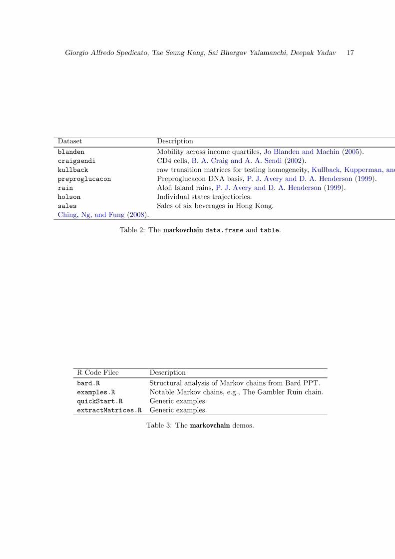
The markovchain package contains some data found in the literature related to DTMC models(see Section 6). Table 2 lists datasets and tables included within the current release of thepackage.
Finally, Table 3 lists the demos included in the demo directory of the package.
Giorgio Alfredo Spedicato, Tae Seung Kang, Sai Bhargav Yalamanchi, Deepak Yadav 17
Dataset Description
blanden Mobility across income quartiles, Jo Blanden and Machin (2005).craigsendi CD4 cells, B. A. Craig and A. A. Sendi (2002).kullback raw transition matrices for testing homogeneity, Kullback, Kupperman, and Ku (1962).preproglucacon Preproglucacon DNA basis, P. J. Avery and D. A. Henderson (1999).rain Alofi Island rains, P. J. Avery and D. A. Henderson (1999).holson Individual states trajectiories.sales Sales of six beverages in Hong Kong.Ching, Ng, and Fung (2008).
Table 2: The markovchain data.frame and table.
R Code Filee Description
bard.R Structural analysis of Markov chains from Bard PPT.examples.R Notable Markov chains, e.g., The Gambler Ruin chain.quickStart.R Generic examples.extractMatrices.R Generic examples.
Table 3: The markovchain demos.
18 The markovchain package
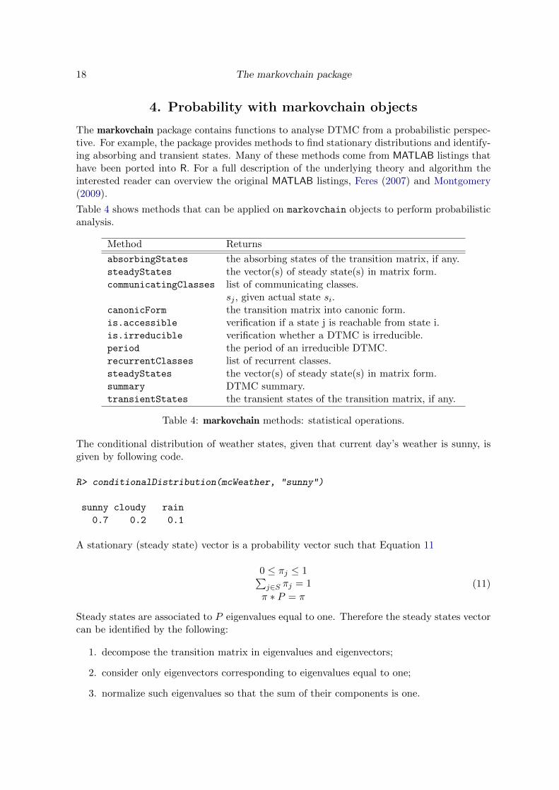
4. Probability with markovchain objects
The markovchain package contains functions to analyse DTMC from a probabilistic perspec-tive. For example, the package provides methods to find stationary distributions and identify-ing absorbing and transient states. Many of these methods come from MATLAB listings thathave been ported into R. For a full description of the underlying theory and algorithm theinterested reader can overview the original MATLAB listings, Feres (2007) and Montgomery(2009).
Table 4 shows methods that can be applied on markovchain objects to perform probabilisticanalysis.
Method Returns
absorbingStates the absorbing states of the transition matrix, if any.steadyStates the vector(s) of steady state(s) in matrix form.communicatingClasses list of communicating classes.
sj , given actual state si.canonicForm the transition matrix into canonic form.is.accessible verification if a state j is reachable from state i.is.irreducible verification whether a DTMC is irreducible.period the period of an irreducible DTMC.recurrentClasses list of recurrent classes.steadyStates the vector(s) of steady state(s) in matrix form.summary DTMC summary.transientStates the transient states of the transition matrix, if any.
Table 4: markovchain methods: statistical operations.
The conditional distribution of weather states, given that current day’s weather is sunny, isgiven by following code.
R> conditionalDistribution(mcWeather, "sunny")
sunny cloudy rain
0.7 0.2 0.1
A stationary (steady state) vector is a probability vector such that Equation 11
0 ≤ πj ≤ 1∑j∈S πj = 1
π ∗ P = π
(11)
Steady states are associated to P eigenvalues equal to one. Therefore the steady states vectorcan be identified by the following:
1. decompose the transition matrix in eigenvalues and eigenvectors;
2. consider only eigenvectors corresponding to eigenvalues equal to one;
3. normalize such eigenvalues so that the sum of their components is one.
Giorgio Alfredo Spedicato, Tae Seung Kang, Sai Bhargav Yalamanchi, Deepak Yadav 19
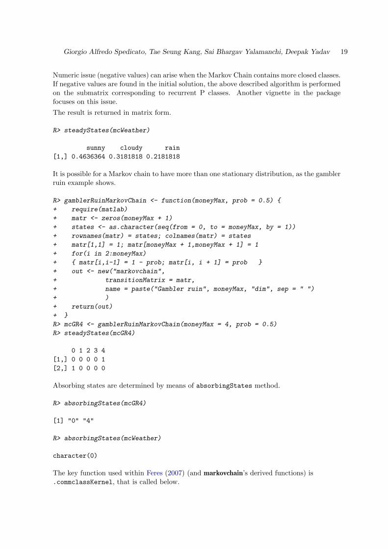
Numeric issue (negative values) can arise when the Markov Chain contains more closed classes.If negative values are found in the initial solution, the above described algorithm is performedon the submatrix corresponding to recurrent P classes. Another vignette in the packagefocuses on this issue.
The result is returned in matrix form.
R> steadyStates(mcWeather)
sunny cloudy rain
[1,] 0.4636364 0.3181818 0.2181818
It is possible for a Markov chain to have more than one stationary distribution, as the gamblerruin example shows.
R> gamblerRuinMarkovChain <- function(moneyMax, prob = 0.5) {
+ require(matlab)
+ matr <- zeros(moneyMax + 1)
+ states <- as.character(seq(from = 0, to = moneyMax, by = 1))
+ rownames(matr) = states; colnames(matr) = states
+ matr[1,1] = 1; matr[moneyMax + 1,moneyMax + 1] = 1
+ for(i in 2:moneyMax)
+ { matr[i,i-1] = 1 - prob; matr[i, i + 1] = prob }
+ out <- new("markovchain",
+ transitionMatrix = matr,
+ name = paste("Gambler ruin", moneyMax, "dim", sep = " ")
+ )
+ return(out)
+ }
R> mcGR4 <- gamblerRuinMarkovChain(moneyMax = 4, prob = 0.5)
R> steadyStates(mcGR4)
0 1 2 3 4
[1,] 0 0 0 0 1
[2,] 1 0 0 0 0
Absorbing states are determined by means of absorbingStates method.
R> absorbingStates(mcGR4)
[1] "0" "4"
R> absorbingStates(mcWeather)
character(0)
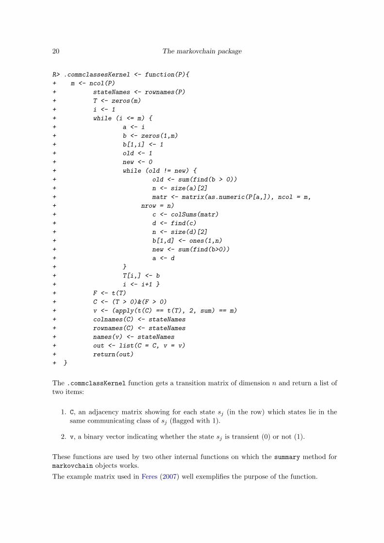
The key function used within Feres (2007) (and markovchain’s derived functions) is.commclassKernel, that is called below.
20 The markovchain package
R> .commclassesKernel <- function(P){
+ m <- ncol(P)
+ stateNames <- rownames(P)
+ T <- zeros(m)
+ i <- 1
+ while (i <= m) {
+ a <- i
+ b <- zeros(1,m)
+ b[1,i] <- 1
+ old <- 1
+ new <- 0
+ while (old != new) {
+ old <- sum(find(b > 0))
+ n <- size(a)[2]
+ matr <- matrix(as.numeric(P[a,]), ncol = m,
+ nrow = n)
+ c <- colSums(matr)
+ d <- find(c)
+ n <- size(d)[2]
+ b[1,d] <- ones(1,n)
+ new <- sum(find(b>0))
+ a <- d
+ }
+ T[i,] <- b
+ i <- i+1 }
+ F <- t(T)
+ C <- (T > 0)&(F > 0)
+ v <- (apply(t(C) == t(T), 2, sum) == m)
+ colnames(C) <- stateNames
+ rownames(C) <- stateNames
+ names(v) <- stateNames
+ out <- list(C = C, v = v)
+ return(out)
+ }
The .commclassKernel function gets a transition matrix of dimension n and return a list oftwo items:
1. C, an adjacency matrix showing for each state sj (in the row) which states lie in thesame communicating class of sj (flagged with 1).
2. v, a binary vector indicating whether the state sj is transient (0) or not (1).
These functions are used by two other internal functions on which the summary method formarkovchain objects works.
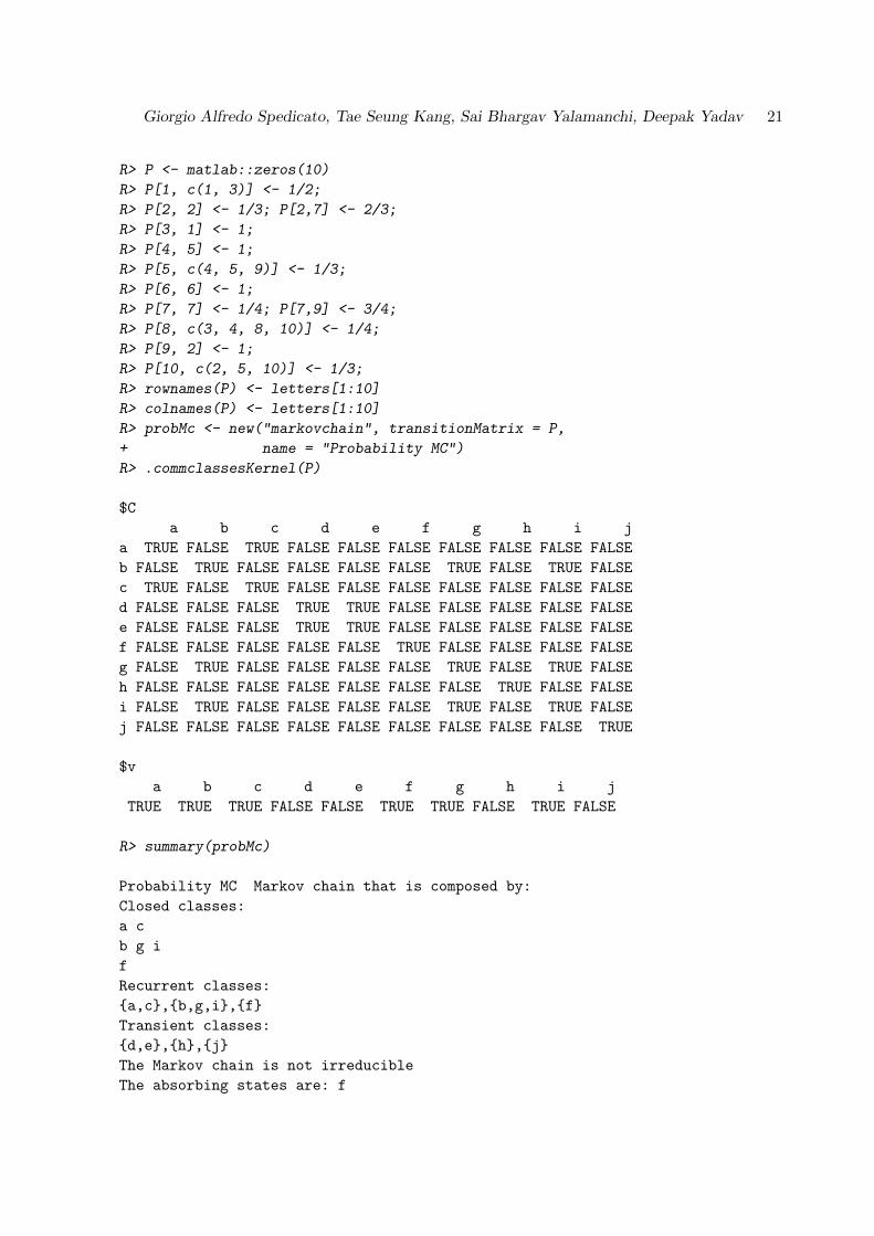
The example matrix used in Feres (2007) well exemplifies the purpose of the function.
Giorgio Alfredo Spedicato, Tae Seung Kang, Sai Bhargav Yalamanchi, Deepak Yadav 21
R> P <- matlab::zeros(10)
R> P[1, c(1, 3)] <- 1/2;
R> P[2, 2] <- 1/3; P[2,7] <- 2/3;
R> P[3, 1] <- 1;
R> P[4, 5] <- 1;
R> P[5, c(4, 5, 9)] <- 1/3;
R> P[6, 6] <- 1;
R> P[7, 7] <- 1/4; P[7,9] <- 3/4;
R> P[8, c(3, 4, 8, 10)] <- 1/4;
R> P[9, 2] <- 1;
R> P[10, c(2, 5, 10)] <- 1/3;
R> rownames(P) <- letters[1:10]
R> colnames(P) <- letters[1:10]
R> probMc <- new("markovchain", transitionMatrix = P,
+ name = "Probability MC")
R> .commclassesKernel(P)
$C
a b c d e f g h i j
a TRUE FALSE TRUE FALSE FALSE FALSE FALSE FALSE FALSE FALSE
b FALSE TRUE FALSE FALSE FALSE FALSE TRUE FALSE TRUE FALSE
c TRUE FALSE TRUE FALSE FALSE FALSE FALSE FALSE FALSE FALSE
d FALSE FALSE FALSE TRUE TRUE FALSE FALSE FALSE FALSE FALSE
e FALSE FALSE FALSE TRUE TRUE FALSE FALSE FALSE FALSE FALSE
f FALSE FALSE FALSE FALSE FALSE TRUE FALSE FALSE FALSE FALSE
g FALSE TRUE FALSE FALSE FALSE FALSE TRUE FALSE TRUE FALSE
h FALSE FALSE FALSE FALSE FALSE FALSE FALSE TRUE FALSE FALSE
i FALSE TRUE FALSE FALSE FALSE FALSE TRUE FALSE TRUE FALSE
j FALSE FALSE FALSE FALSE FALSE FALSE FALSE FALSE FALSE TRUE
$v
a b c d e f g h i j
TRUE TRUE TRUE FALSE FALSE TRUE TRUE FALSE TRUE FALSE
R> summary(probMc)
Probability MC Markov chain that is composed by:
Closed classes:
a c
b g i
f
Recurrent classes:
{a,c},{b,g,i},{f}
Transient classes:
{d,e},{h},{j}
The Markov chain is not irreducible
The absorbing states are: f
22 The markovchain package
All states that pertain to a transient class are named ”transient” and a specific method hasbeen written to elicit them.
R> transientStates(probMc)
[1] "d" "e" "h" "j"
Listings from Feres (2007) have been adapted into canonicForm method that turns a Markovchain into canonic form.
R> probMcCanonic <- canonicForm(probMc)
R> probMc
Probability MC
A 10 - dimensional discrete Markov Chain defined by the following states:
a, b, c, d, e, f, g, h, i, j
The transition matrix (by rows) is defined as follows:
a b c d e f g h i
a 0.5 0.0000000 0.50 0.0000000 0.0000000 0 0.0000000 0.00 0.0000000
b 0.0 0.3333333 0.00 0.0000000 0.0000000 0 0.6666667 0.00 0.0000000
c 1.0 0.0000000 0.00 0.0000000 0.0000000 0 0.0000000 0.00 0.0000000
d 0.0 0.0000000 0.00 0.0000000 1.0000000 0 0.0000000 0.00 0.0000000
e 0.0 0.0000000 0.00 0.3333333 0.3333333 0 0.0000000 0.00 0.3333333
f 0.0 0.0000000 0.00 0.0000000 0.0000000 1 0.0000000 0.00 0.0000000
g 0.0 0.0000000 0.00 0.0000000 0.0000000 0 0.2500000 0.00 0.7500000
h 0.0 0.0000000 0.25 0.2500000 0.0000000 0 0.0000000 0.25 0.0000000
i 0.0 1.0000000 0.00 0.0000000 0.0000000 0 0.0000000 0.00 0.0000000
j 0.0 0.3333333 0.00 0.0000000 0.3333333 0 0.0000000 0.00 0.0000000
j
a 0.0000000
b 0.0000000
c 0.0000000
d 0.0000000
e 0.0000000
f 0.0000000
g 0.0000000
h 0.2500000
i 0.0000000
j 0.3333333
R> probMcCanonic
Probability MC
A 10 - dimensional discrete Markov Chain defined by the following states:
a, c, b, g, i, f, d, e, h, j
The transition matrix (by rows) is defined as follows:
Giorgio Alfredo Spedicato, Tae Seung Kang, Sai Bhargav Yalamanchi, Deepak Yadav 23
a c b g i f d e h
a 0.5 0.50 0.0000000 0.0000000 0.0000000 0 0.0000000 0.0000000 0.00
c 1.0 0.00 0.0000000 0.0000000 0.0000000 0 0.0000000 0.0000000 0.00
b 0.0 0.00 0.3333333 0.6666667 0.0000000 0 0.0000000 0.0000000 0.00
g 0.0 0.00 0.0000000 0.2500000 0.7500000 0 0.0000000 0.0000000 0.00
i 0.0 0.00 1.0000000 0.0000000 0.0000000 0 0.0000000 0.0000000 0.00
f 0.0 0.00 0.0000000 0.0000000 0.0000000 1 0.0000000 0.0000000 0.00
d 0.0 0.00 0.0000000 0.0000000 0.0000000 0 0.0000000 1.0000000 0.00
e 0.0 0.00 0.0000000 0.0000000 0.3333333 0 0.3333333 0.3333333 0.00
h 0.0 0.25 0.0000000 0.0000000 0.0000000 0 0.2500000 0.0000000 0.25
j 0.0 0.00 0.3333333 0.0000000 0.0000000 0 0.0000000 0.3333333 0.00
j
a 0.0000000
c 0.0000000
b 0.0000000
g 0.0000000
i 0.0000000
f 0.0000000
d 0.0000000
e 0.0000000
h 0.2500000
j 0.3333333
The function is.accessible permits to investigate whether a state sj is accessible from statesi, that is whether the probability to eventually reach sj starting from si is greater than zero.
R> is.accessible(object = probMc, from = "a", to = "c")
[1] TRUE
R> is.accessible(object = probMc, from = "g", to = "c")
[1] FALSE
In Section 2.2 we observed that, if a DTMC is irreducible, all its states share the sameperiodicity. Then, the period function returns the periodicity of the DTMC, provided thatit is irreducible. The example that follows shows how to find if a DTMC is reducible orirreducible by means of the function is.irreducible and, in the latter case, the methodperiod is used to compute the periodicity of the chain.
R> E <- matrix(0, nrow = 4, ncol = 4)
R> E[1, 2] <- 1
R> E[2, 1] <- 1/3; E[2, 3] <- 2/3
R> E[3,2] <- 1/4; E[3, 4] <- 3/4
R> E[4, 3] <- 1
R> mcE <- new("markovchain", states = c("a", "b", "c", "d"),
24 The markovchain package
+ transitionMatrix = E,
+ name = "E")
R> is.irreducible(mcE)
[1] TRUE
R> period(mcE)
[1] 2
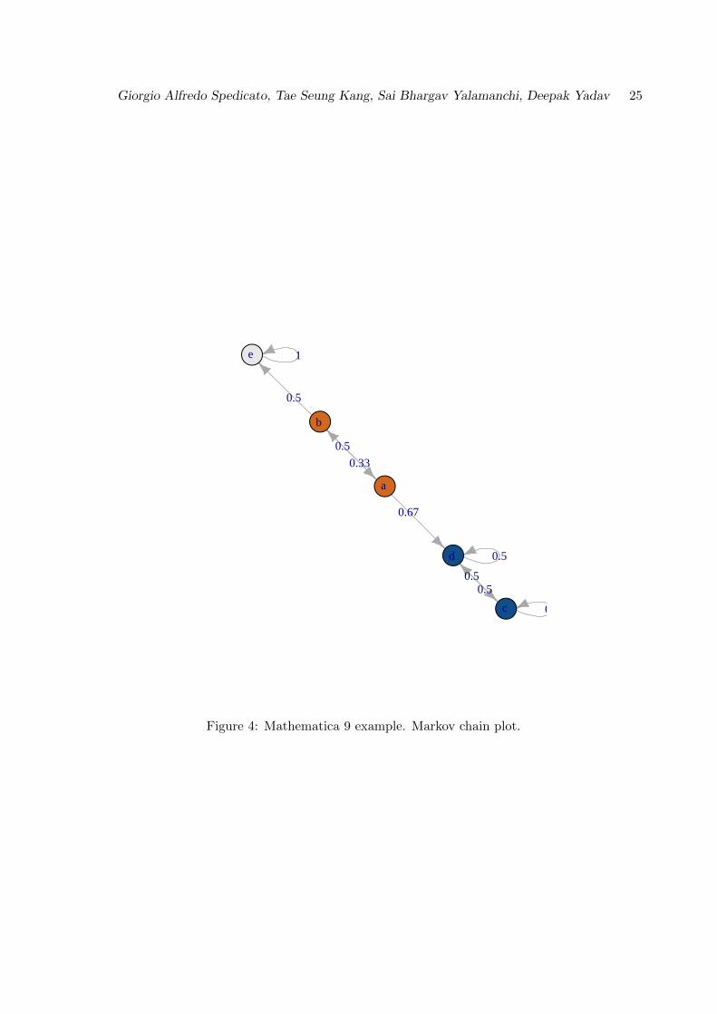
The example Markov chain found in Mathematica web site (Wolfram Research 2013a) hasbeen used, and is plotted in Figure 4.
R> require(matlab)
R> mathematicaMatr <- zeros(5)
R> mathematicaMatr[1,] <- c(0, 1/3, 0, 2/3, 0)
R> mathematicaMatr[2,] <- c(1/2, 0, 0, 0, 1/2)
R> mathematicaMatr[3,] <- c(0, 0, 1/2, 1/2, 0)
R> mathematicaMatr[4,] <- c(0, 0, 1/2, 1/2, 0)
R> mathematicaMatr[5,] <- c(0, 0, 0, 0, 1)
R> statesNames <- letters[1:5]
R> mathematicaMc <- new("markovchain", transitionMatrix = mathematicaMatr,
+ name = "Mathematica MC", states = statesNames)
Mathematica MC Markov chain that is composed by:
Closed classes:
c d
e
Recurrent classes:
{c,d},{e}
Transient classes:
{a,b}
The Markov chain is not irreducible
The absorbing states are: e
Feres (2007) provides code to compute first passage time (within 1, 2, . . . , n steps) given theinitial state to be i. The MATLAB listings translated into R on which the firstPassage
function is based are
R> .firstpassageKernel <- function(P, i, n){
+ G <- P
+ H <- P[i,]
+ E <- 1 - diag(size(P)[2])
+ for (m in 2:n) {
+ G <- P %*% (G * E)
Giorgio Alfredo Spedicato, Tae Seung Kang, Sai Bhargav Yalamanchi, Deepak Yadav 25
0.5
0.5
1
0.33
0.67
0.5
0.5
0.50.5
●
●
●
●
●
a
b
c
d
e
Figure 4: Mathematica 9 example. Markov chain plot.
26 The markovchain package
+ H <- rbind(H, G[i,])
+ }
+ return(H)
+ }
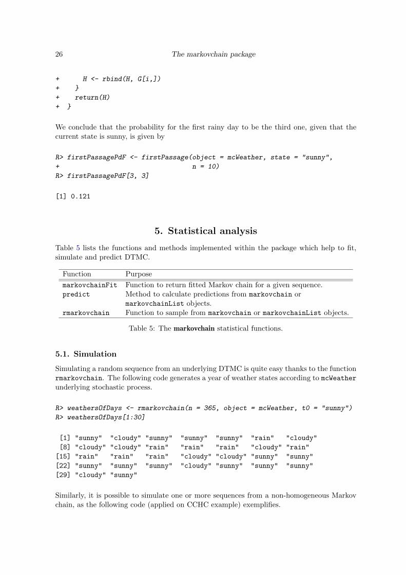
We conclude that the probability for the first rainy day to be the third one, given that thecurrent state is sunny, is given by
R> firstPassagePdF <- firstPassage(object = mcWeather, state = "sunny",
+ n = 10)
R> firstPassagePdF[3, 3]
[1] 0.121
5. Statistical analysis
Table 5 lists the functions and methods implemented within the package which help to fit,simulate and predict DTMC.
Function Purpose
markovchainFit Function to return fitted Markov chain for a given sequence.predict Method to calculate predictions from markovchain or
markovchainList objects.rmarkovchain Function to sample from markovchain or markovchainList objects.
Table 5: The markovchain statistical functions.
5.1. Simulation
Simulating a random sequence from an underlying DTMC is quite easy thanks to the functionrmarkovchain. The following code generates a year of weather states according to mcWeather
underlying stochastic process.
R> weathersOfDays <- rmarkovchain(n = 365, object = mcWeather, t0 = "sunny")
R> weathersOfDays[1:30]
[1] "sunny" "cloudy" "sunny" "sunny" "sunny" "rain" "cloudy"
[8] "cloudy" "cloudy" "rain" "rain" "rain" "cloudy" "rain"
[15] "rain" "rain" "rain" "cloudy" "cloudy" "sunny" "sunny"
[22] "sunny" "sunny" "sunny" "cloudy" "sunny" "sunny" "sunny"
[29] "cloudy" "sunny"
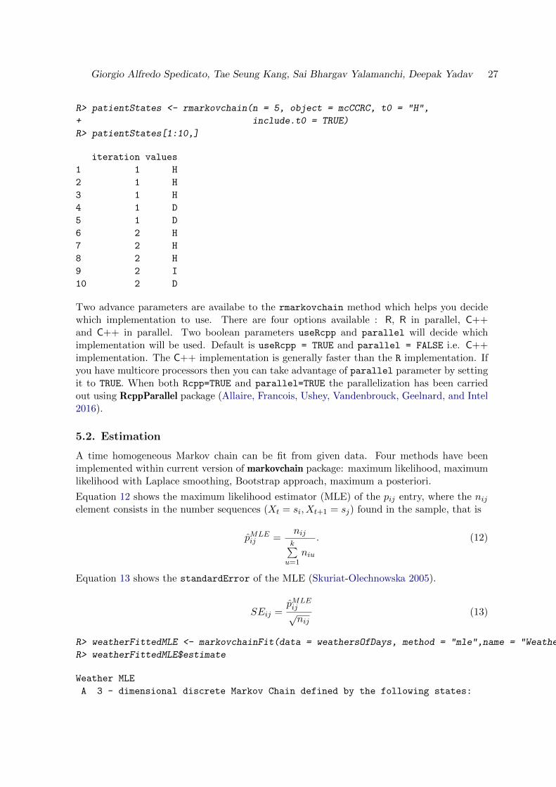
Similarly, it is possible to simulate one or more sequences from a non-homogeneous Markovchain, as the following code (applied on CCHC example) exemplifies.
Giorgio Alfredo Spedicato, Tae Seung Kang, Sai Bhargav Yalamanchi, Deepak Yadav 27
R> patientStates <- rmarkovchain(n = 5, object = mcCCRC, t0 = "H",
+ include.t0 = TRUE)
R> patientStates[1:10,]
iteration values
1 1 H
2 1 H
3 1 H
4 1 D
5 1 D
6 2 H
7 2 H
8 2 H
9 2 I
10 2 D
Two advance parameters are availabe to the rmarkovchain method which helps you decidewhich implementation to use. There are four options available : R, R in parallel, C++and C++ in parallel. Two boolean parameters useRcpp and parallel will decide whichimplementation will be used. Default is useRcpp = TRUE and parallel = FALSE i.e. C++implementation. The C++ implementation is generally faster than the R implementation. Ifyou have multicore processors then you can take advantage of parallel parameter by settingit to TRUE. When both Rcpp=TRUE and parallel=TRUE the parallelization has been carriedout using RcppParallel package (Allaire, Francois, Ushey, Vandenbrouck, Geelnard, and Intel2016).
5.2. Estimation
A time homogeneous Markov chain can be fit from given data. Four methods have beenimplemented within current version of markovchain package: maximum likelihood, maximumlikelihood with Laplace smoothing, Bootstrap approach, maximum a posteriori.
Equation 12 shows the maximum likelihood estimator (MLE) of the pij entry, where the nijelement consists in the number sequences (Xt = si, Xt+1 = sj) found in the sample, that is
pMLEij =
nijk∑
u=1niu
. (12)
Equation 13 shows the standardError of the MLE (Skuriat-Olechnowska 2005).
SEij =pMLEij√nij
(13)
R> weatherFittedMLE <- markovchainFit(data = weathersOfDays, method = "mle",name = "Weather MLE")
R> weatherFittedMLE$estimate
Weather MLE
A 3 - dimensional discrete Markov Chain defined by the following states:
28 The markovchain package
cloudy, rain, sunny
The transition matrix (by rows) is defined as follows:
cloudy rain sunny
cloudy 0.4067797 0.33898305 0.2542373
rain 0.4315789 0.42105263 0.1473684
sunny 0.1920530 0.09933775 0.7086093
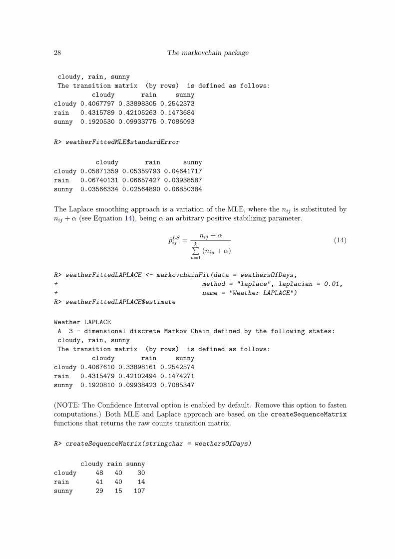
R> weatherFittedMLE$standardError
cloudy rain sunny
cloudy 0.05871359 0.05359793 0.04641717
rain 0.06740131 0.06657427 0.03938587
sunny 0.03566334 0.02564890 0.06850384
The Laplace smoothing approach is a variation of the MLE, where the nij is substituted bynij + α (see Equation 14), being α an arbitrary positive stabilizing parameter.
pLSij =nij + α
k∑u=1
(niu + α)
(14)
R> weatherFittedLAPLACE <- markovchainFit(data = weathersOfDays,
+ method = "laplace", laplacian = 0.01,
+ name = "Weather LAPLACE")
R> weatherFittedLAPLACE$estimate
Weather LAPLACE
A 3 - dimensional discrete Markov Chain defined by the following states:
cloudy, rain, sunny
The transition matrix (by rows) is defined as follows:
cloudy rain sunny
cloudy 0.4067610 0.33898161 0.2542574
rain 0.4315479 0.42102494 0.1474271
sunny 0.1920810 0.09938423 0.7085347
(NOTE: The Confidence Interval option is enabled by default. Remove this option to fastencomputations.) Both MLE and Laplace approach are based on the createSequenceMatrix
functions that returns the raw counts transition matrix.
R> createSequenceMatrix(stringchar = weathersOfDays)
cloudy rain sunny
cloudy 48 40 30
rain 41 40 14
sunny 29 15 107
Giorgio Alfredo Spedicato, Tae Seung Kang, Sai Bhargav Yalamanchi, Deepak Yadav 29
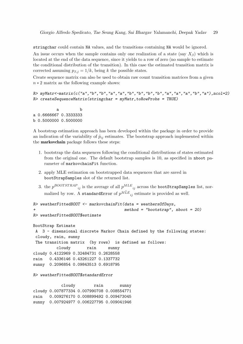
stringchar could contain NA values, and the transitions containing NA would be ignored.
An issue occurs when the sample contains only one realization of a state (say Xβ) which islocated at the end of the data sequence, since it yields to a row of zero (no sample to estimatethe conditional distribution of the transition). In this case the estimated transition matrix iscorrected assuming pβ,j = 1/k, being k the possible states.
Create sequence matrix can also be used to obtain raw count transition matrices from a givenn ∗ 2 matrix as the following example shows:
R> myMatr<-matrix(c("a","b","b","a","a","b","b","b","b","a","a","a","b","a"),ncol=2)
R> createSequenceMatrix(stringchar = myMatr,toRowProbs = TRUE)
a b
a 0.6666667 0.3333333
b 0.5000000 0.5000000
A bootstrap estimation approach has been developed within the package in order to providean indication of the variability of pij estimates. The bootstrap approach implemented withinthe markovchain package follows these steps:
1. bootstrap the data sequences following the conditional distributions of states estimatedfrom the original one. The default bootstrap samples is 10, as specified in nboot pa-rameter of markovchainFit function.
2. apply MLE estimation on bootstrapped data sequences that are saved inbootStrapSamples slot of the returned list.
3. the pBOOTSTRAP ij is the average of all pMLEij across the bootStrapSamples list, nor-
malized by row. A standardError of ˆpMLEij estimate is provided as well.
R> weatherFittedBOOT <- markovchainFit(data = weathersOfDays,
+ method = "bootstrap", nboot = 20)
R> weatherFittedBOOT$estimate
BootStrap Estimate
A 3 - dimensional discrete Markov Chain defined by the following states:
cloudy, rain, sunny
The transition matrix (by rows) is defined as follows:
cloudy rain sunny
cloudy 0.4122969 0.32484731 0.2628558
rain 0.4336146 0.43261227 0.1337732
sunny 0.2096854 0.09843513 0.6918795
R> weatherFittedBOOT$standardError
cloudy rain sunny
cloudy 0.007877334 0.007990708 0.008554771
rain 0.009276170 0.008899492 0.009473045
sunny 0.007924977 0.006227795 0.009041946
30 The markovchain package
The bootstrapping process can be done in parallel thanks to RcppParallel package (Allaireet al. 2016). Parallelized implementation is definitively suggested when the data sample sizeor the required number of bootstrap runs is high.
R> weatherFittedBOOTParallel <- markovchainFit(data = weathersOfDays,
+ method = "bootstrap", nboot = 200,
+ parallel = TRUE)
R> weatherFittedBOOTParallel$estimate
R> weatherFittedBOOTParallel$standardError
The parallel bootstrapping uses all the available cores on a machine by default. However, it isalso possible to tune the number of threads used. Note that this should be done in R beforecalling the markovchainFit function. For example, the following code will set the number ofthreads to 4.
R> RcppParallel::setNumThreads(2)
For more details, please refer to RcppParallel web site.
For all the fitting methods, the logLikelihood (Skuriat-Olechnowska 2005) denoted in Equa-tion 15 is provided.
LLH =∑i,j
nij ∗ log(pij) (15)
where nij is the entry of the frequency matrix and pij is the entry of the transition probabilitymatrix.
R> weatherFittedMLE$logLikelihood
[1] -342.7361
R> weatherFittedBOOT$logLikelihood
[1] -343.0181
Confidence matrices of estimated parameters (parametric for MLE, non - parametric forBootStrap) are available as well. The confidenceInterval is provided with the two matrices:lowerEndpointMatrix and upperEndpointMatrix. The confidence level (CL) is 0.95 bydefault and can be given as an argument of the function markovchainFit. This is usedto obtain the standard score (z-score). Equations 16 and 17 (Skuriat-Olechnowska 2005)show the confidenceInterval of a fitting. Note that each entry of the matrices is boundedbetween 0 and 1.
LowerEndpointij = pij − zscore(CL) ∗ SEij (16)
UpperEndpointij = pij + zscore(CL) ∗ SEij (17)
Giorgio Alfredo Spedicato, Tae Seung Kang, Sai Bhargav Yalamanchi, Deepak Yadav 31
R> weatherFittedMLE$confidenceInterval
NULL
R> weatherFittedBOOT$confidenceInterval
$confidenceLevel
[1] 0.95
$lowerEndpointMatrix
cloudy rain sunny
cloudy 0.3993398 0.31170376 0.2487845
rain 0.4183566 0.41797391 0.1181914
sunny 0.1966500 0.08819132 0.6770068
$upperEndpointMatrix
cloudy rain sunny
cloudy 0.4252539 0.3379909 0.2769272
rain 0.4488725 0.4472506 0.1493549
sunny 0.2227208 0.1086789 0.7067522
A special function, multinomialConfidenceIntervals, has been written in order to obtainmultinomial wise confidence intervals. The code has been based on and Rcpp translation ofpackage’s MultinomialCI functions Villacorta (2012) that were themselves based on the Sisonand Glaz (1995) paper.
R> multinomialConfidenceIntervals(transitionMatrix =
+ weatherFittedMLE$estimate@transitionMatrix,
+ countsTransitionMatrix = createSequenceMatrix(weathersOfDays))
$confidenceLevel
[1] 0.95
$lowerEndpointMatrix
cloudy rain sunny
cloudy 0.3135593 0.24576271 0.16101695
rain 0.3368421 0.32631579 0.05263158
sunny 0.1258278 0.03311258 0.64238411
$upperEndpointMatrix
cloudy rain sunny
cloudy 0.5066571 0.4388605 0.3541147
rain 0.5460851 0.5355588 0.2618746
sunny 0.2665208 0.1738056 0.7830771
The functions for fitting DTMC have mostly been rewritten in C++ using Rcpp Eddelbuettel(2013) since version 0.2.
32 The markovchain package
It is also possible to fit a DTMC object from matrix or data.frame objects as shown infollowing code.
R> data(holson)
R> singleMc<-markovchainFit(data=holson[,2:12],name="holson")
The same applies for markovchainList.
R> mcListFit<-markovchainListFit(data=holson[,2:6],name="holson")
R> mcListFit$estimate
holson list of Markov chain(s)
Markovchain 1
Unnamed Markov chain
A 3 - dimensional discrete Markov Chain defined by the following states:
1, 2, 3
The transition matrix (by rows) is defined as follows:
1 2 3
1 0.94609164 0.05390836 0.0000000
2 0.26356589 0.62790698 0.1085271
3 0.02325581 0.18604651 0.7906977
Markovchain 2
Unnamed Markov chain
A 3 - dimensional discrete Markov Chain defined by the following states:
1, 2, 3
The transition matrix (by rows) is defined as follows:
1 2 3
1 0.9323410 0.0676590 0.0000000
2 0.2551724 0.5103448 0.2344828
3 0.0000000 0.0862069 0.9137931
Markovchain 3
Unnamed Markov chain
A 3 - dimensional discrete Markov Chain defined by the following states:
1, 2, 3
The transition matrix (by rows) is defined as follows:
1 2 3
1 0.94765840 0.04820937 0.004132231
2 0.26119403 0.66417910 0.074626866
3 0.01428571 0.13571429 0.850000000
Markovchain 4
Unnamed Markov chain
A 3 - dimensional discrete Markov Chain defined by the following states:
1, 2, 3
The transition matrix (by rows) is defined as follows:
Giorgio Alfredo Spedicato, Tae Seung Kang, Sai Bhargav Yalamanchi, Deepak Yadav 33
1 2 3
1 0.9172414 0.07724138 0.005517241
2 0.1678322 0.60839161 0.223776224
3 0.0000000 0.03030303 0.969696970
Finally, given a list object, it is possible to fit a markovchain object or to obtain the rawtransition matrix.
R> c1<-c("a","b","a","a","c","c","a")
R> c2<-c("b")
R> c3<-c("c","a","a","c")
R> c4<-c("b","a","b","a","a","c","b")
R> c5<-c("a","a","c",NA)
R> c6<-c("b","c","b","c","a")
R> mylist<-list(c1,c2,c3,c4,c5,c6)
R> mylistMc<-markovchainFit(data=mylist)
R> mylistMc
$estimate
MLE Fit
A 3 - dimensional discrete Markov Chain defined by the following states:
a, b, c
The transition matrix (by rows) is defined as follows:
a b c
a 0.4 0.2000000 0.4000000
b 0.6 0.0000000 0.4000000
c 0.5 0.3333333 0.1666667
$standardError
a b c
a 0.2000000 0.1414214 0.2000000
b 0.3464102 0.0000000 0.2828427
c 0.2886751 0.2357023 0.1666667
$confidenceLevel
[1] 0.95
$lowerEndpointMatrix
a b c
a 0.07102927 0 0.07102927
b 0.03020599 0 0.00000000
c 0.02517166 0 0.00000000
$upperEndpointMatrix
a b c
a 0.7289707 0.4326174 0.7289707
34 The markovchain package
b 1.0000000 0.0000000 0.8652349
c 0.9748283 0.7210291 0.4408089
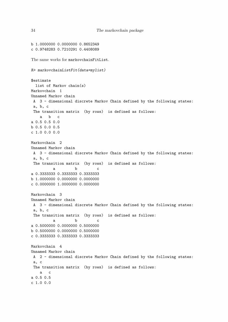
The same works for markovchainFitList.
R> markovchainListFit(data=mylist)
$estimate
list of Markov chain(s)
Markovchain 1
Unnamed Markov chain
A 3 - dimensional discrete Markov Chain defined by the following states:
a, b, c
The transition matrix (by rows) is defined as follows:
a b c
a 0.5 0.5 0.0
b 0.5 0.0 0.5
c 1.0 0.0 0.0
Markovchain 2
Unnamed Markov chain
A 3 - dimensional discrete Markov Chain defined by the following states:
a, b, c
The transition matrix (by rows) is defined as follows:
a b c
a 0.3333333 0.3333333 0.3333333
b 1.0000000 0.0000000 0.0000000
c 0.0000000 1.0000000 0.0000000
Markovchain 3
Unnamed Markov chain
A 3 - dimensional discrete Markov Chain defined by the following states:
a, b, c
The transition matrix (by rows) is defined as follows:
a b c
a 0.5000000 0.0000000 0.5000000
b 0.5000000 0.0000000 0.5000000
c 0.3333333 0.3333333 0.3333333
Markovchain 4
Unnamed Markov chain
A 2 - dimensional discrete Markov Chain defined by the following states:
a, c
The transition matrix (by rows) is defined as follows:
a c
a 0.5 0.5
c 1.0 0.0
Giorgio Alfredo Spedicato, Tae Seung Kang, Sai Bhargav Yalamanchi, Deepak Yadav 35
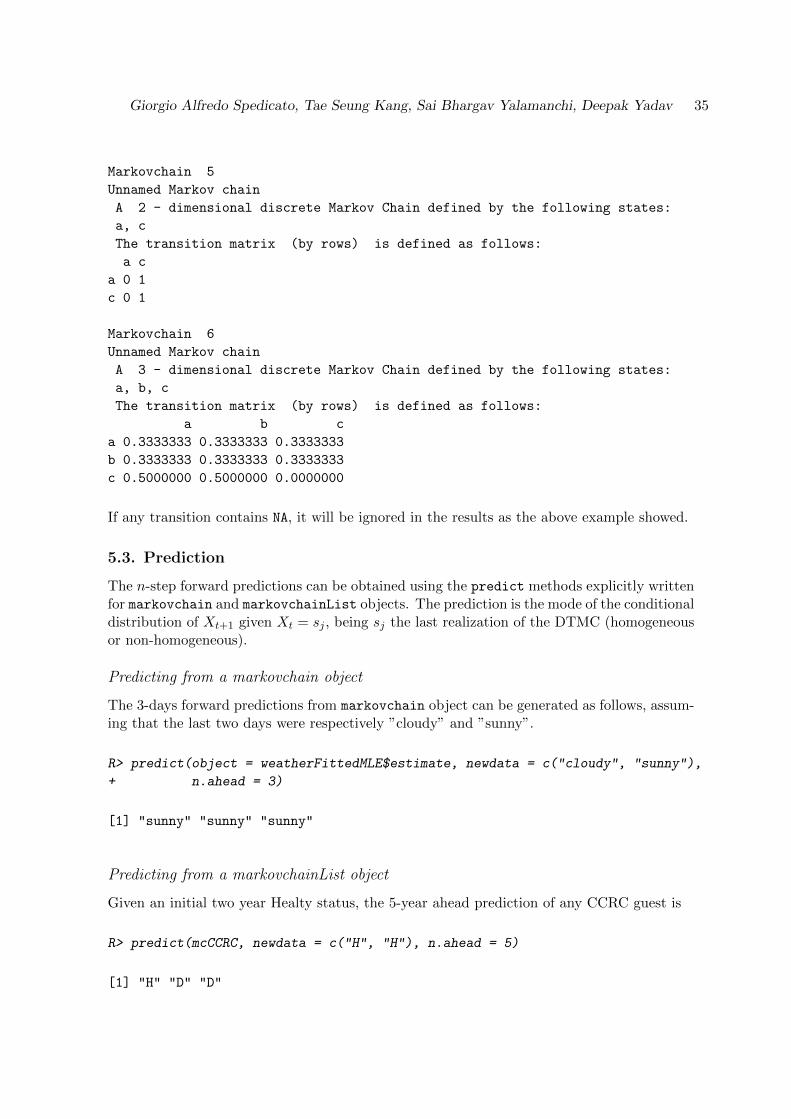
Markovchain 5
Unnamed Markov chain
A 2 - dimensional discrete Markov Chain defined by the following states:
a, c
The transition matrix (by rows) is defined as follows:
a c
a 0 1
c 0 1
Markovchain 6
Unnamed Markov chain
A 3 - dimensional discrete Markov Chain defined by the following states:
a, b, c
The transition matrix (by rows) is defined as follows:
a b c
a 0.3333333 0.3333333 0.3333333
b 0.3333333 0.3333333 0.3333333
c 0.5000000 0.5000000 0.0000000
If any transition contains NA, it will be ignored in the results as the above example showed.
5.3. Prediction
The n-step forward predictions can be obtained using the predict methods explicitly writtenfor markovchain and markovchainList objects. The prediction is the mode of the conditionaldistribution of Xt+1 given Xt = sj , being sj the last realization of the DTMC (homogeneousor non-homogeneous).
Predicting from a markovchain object
The 3-days forward predictions from markovchain object can be generated as follows, assum-ing that the last two days were respectively ”cloudy” and ”sunny”.
R> predict(object = weatherFittedMLE$estimate, newdata = c("cloudy", "sunny"),
+ n.ahead = 3)
[1] "sunny" "sunny" "sunny"
Predicting from a markovchainList object
Given an initial two year Healty status, the 5-year ahead prediction of any CCRC guest is
R> predict(mcCCRC, newdata = c("H", "H"), n.ahead = 5)
[1] "H" "D" "D"
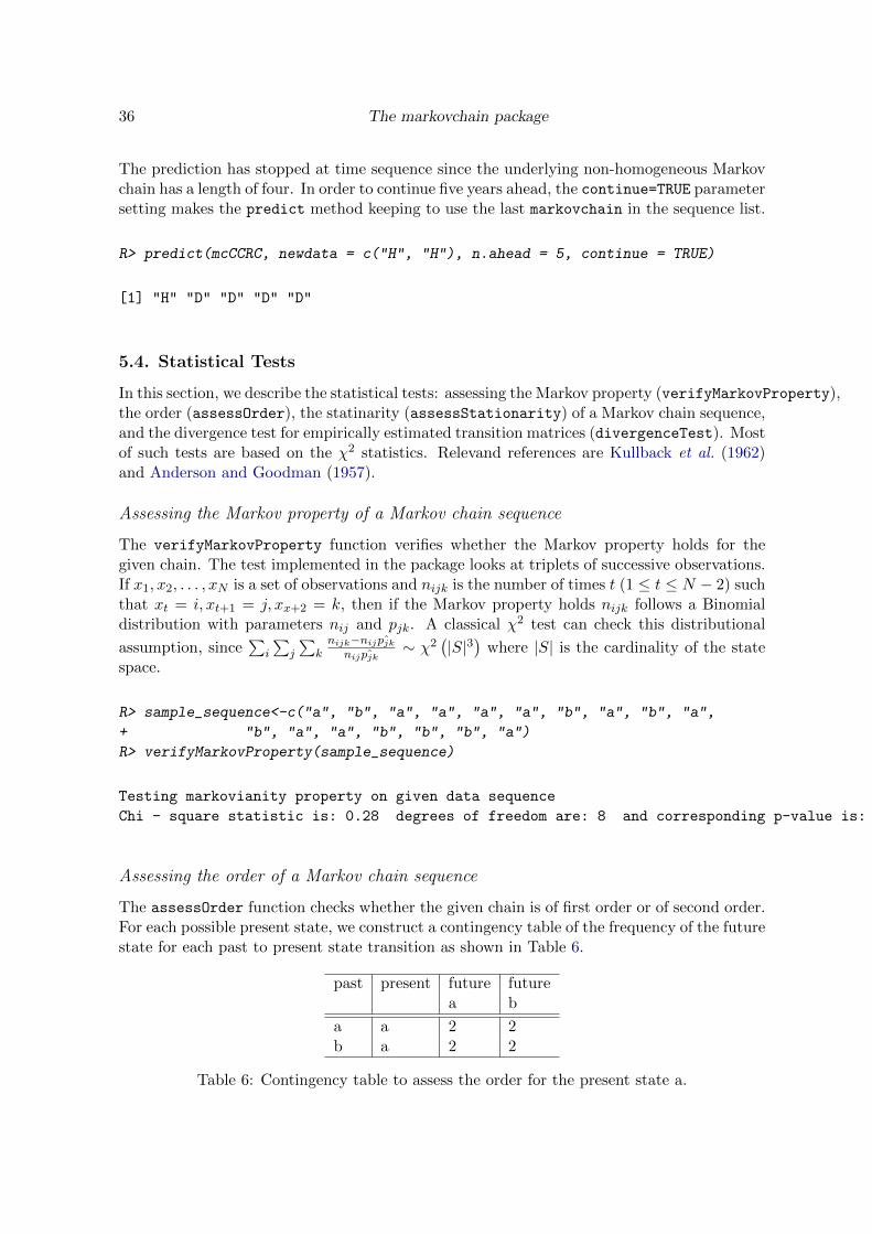
36 The markovchain package
The prediction has stopped at time sequence since the underlying non-homogeneous Markovchain has a length of four. In order to continue five years ahead, the continue=TRUE parametersetting makes the predict method keeping to use the last markovchain in the sequence list.
R> predict(mcCCRC, newdata = c("H", "H"), n.ahead = 5, continue = TRUE)
[1] "H" "D" "D" "D" "D"
5.4. Statistical Tests
In this section, we describe the statistical tests: assessing the Markov property (verifyMarkovProperty),the order (assessOrder), the statinarity (assessStationarity) of a Markov chain sequence,and the divergence test for empirically estimated transition matrices (divergenceTest). Mostof such tests are based on the χ2 statistics. Relevand references are Kullback et al. (1962)and Anderson and Goodman (1957).
Assessing the Markov property of a Markov chain sequence
The verifyMarkovProperty function verifies whether the Markov property holds for thegiven chain. The test implemented in the package looks at triplets of successive observations.If x1, x2, . . . , xN is a set of observations and nijk is the number of times t (1 ≤ t ≤ N − 2) suchthat xt = i, xt+1 = j, xx+2 = k, then if the Markov property holds nijk follows a Binomialdistribution with parameters nij and pjk. A classical χ2 test can check this distributional
assumption, since∑
i
∑j
∑knijk−nij ˆpjk
nij ˆpjk∼ χ2
(|S|3
)where |S| is the cardinality of the state
space.
R> sample_sequence<-c("a", "b", "a", "a", "a", "a", "b", "a", "b", "a",
+ "b", "a", "a", "b", "b", "b", "a")
R> verifyMarkovProperty(sample_sequence)
Testing markovianity property on given data sequence
Chi - square statistic is: 0.28 degrees of freedom are: 8 and corresponding p-value is: 0.9999857
Assessing the order of a Markov chain sequence
The assessOrder function checks whether the given chain is of first order or of second order.For each possible present state, we construct a contingency table of the frequency of the futurestate for each past to present state transition as shown in Table 6.
past present future futurea b
a a 2 2b a 2 2
Table 6: Contingency table to assess the order for the present state a.
Giorgio Alfredo Spedicato, Tae Seung Kang, Sai Bhargav Yalamanchi, Deepak Yadav 37
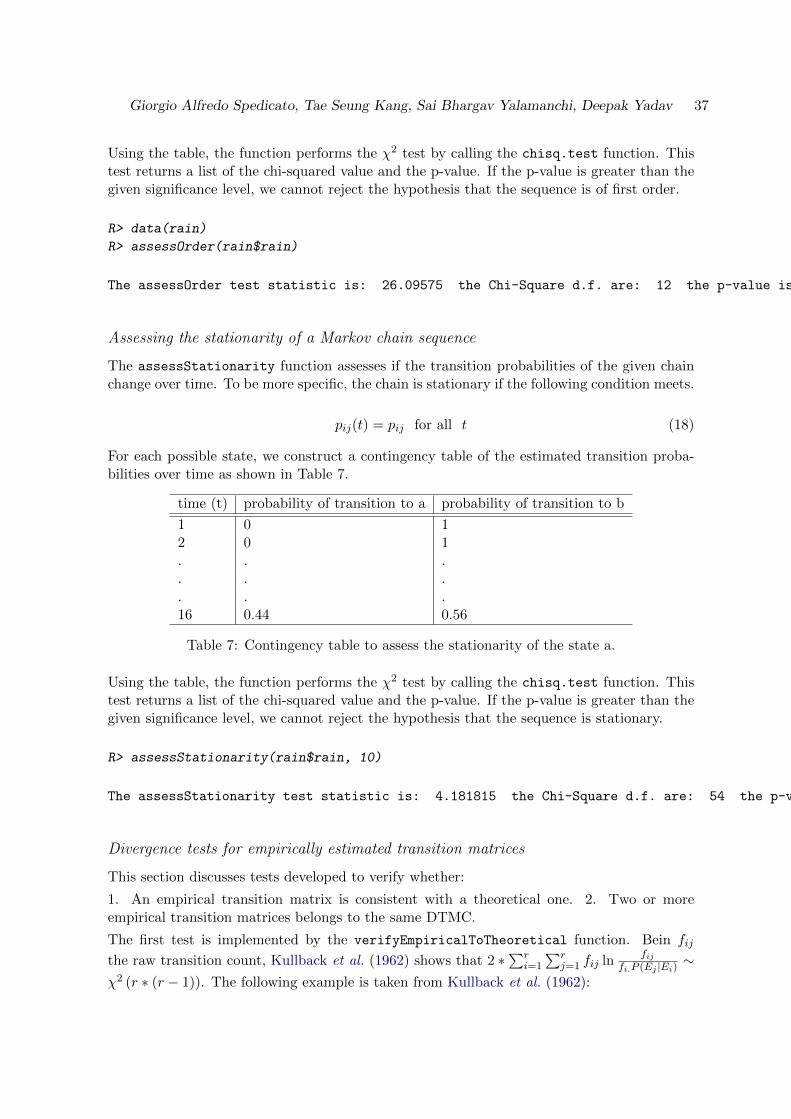
Using the table, the function performs the χ2 test by calling the chisq.test function. Thistest returns a list of the chi-squared value and the p-value. If the p-value is greater than thegiven significance level, we cannot reject the hypothesis that the sequence is of first order.
R> data(rain)
R> assessOrder(rain$rain)
The assessOrder test statistic is: 26.09575 the Chi-Square d.f. are: 12 the p-value is: 0.01040395
Assessing the stationarity of a Markov chain sequence
The assessStationarity function assesses if the transition probabilities of the given chainchange over time. To be more specific, the chain is stationary if the following condition meets.
pij(t) = pij for all t (18)
For each possible state, we construct a contingency table of the estimated transition proba-bilities over time as shown in Table 7.
time (t) probability of transition to a probability of transition to b
1 0 12 0 1. . .. . .. . .16 0.44 0.56
Table 7: Contingency table to assess the stationarity of the state a.
Using the table, the function performs the χ2 test by calling the chisq.test function. Thistest returns a list of the chi-squared value and the p-value. If the p-value is greater than thegiven significance level, we cannot reject the hypothesis that the sequence is stationary.
R> assessStationarity(rain$rain, 10)
The assessStationarity test statistic is: 4.181815 the Chi-Square d.f. are: 54 the p-value is: 1
Divergence tests for empirically estimated transition matrices
This section discusses tests developed to verify whether:
1. An empirical transition matrix is consistent with a theoretical one. 2. Two or moreempirical transition matrices belongs to the same DTMC.
The first test is implemented by the verifyEmpiricalToTheoretical function. Bein fij
the raw transition count, Kullback et al. (1962) shows that 2 ∗∑r
i=1
∑rj=1 fij ln
fijfi.P (Ej |Ei)
∼χ2 (r ∗ (r − 1)). The following example is taken from Kullback et al. (1962):

38 The markovchain package
R> sequence<-c(0,1,2,2,1,0,0,0,0,0,0,1,2,2,2,1,0,0,1,0,0,0,0,0,0,1,1,
+ 2,0,0,2,1,1,0,0,0,0,0,0,0,0,0,0,0,0,0,0,1,1,1,1,0,0,0,0,2,1,0,
+ 0,2,1,0,0,0,0,0,0,1,1,1,2,2,0,0,2,1,1,1,1,2,1,1,1,1,1,1,1,1,1,0,2,
+ 0,1,1,0,0,0,1,2,2,0,0,0,0,0,0,2,2,2,1,1,1,1,0,1,1,1,1,0,0,2,1,1,
+ 0,0,0,0,0,2,2,1,1,1,1,1,2,1,2,0,0,0,1,2,2,2,0,0,0,1,1)
R> mc=matrix(c(5/8,1/4,1/8,1/4,1/2,1/4,1/4,3/8,3/8),byrow=TRUE, nrow=3)
R> rownames(mc)<-colnames(mc)<-0:2; theoreticalMc<-as(mc, "markovchain")
R> verifyEmpiricalToTheoretical(data=sequence,object=theoreticalMc)
Testing whether the
0 1 2
0 51 11 8
1 12 31 9
2 6 11 10
transition matrix is compatible with
0 1 2
0 0.625 0.250 0.125
1 0.250 0.500 0.250
2 0.250 0.375 0.375
[1] "theoretical transition matrix"
ChiSq statistic is 6.551795 d.o.f are 6 corresponding p-value is 0.3642899
$statistic
0
6.551795
$dof
[1] 6
$pvalue
0
0.3642899
The second one is implemented by the verifyHomogeneity function, inspired by (Kullbacket al. 1962, section 9). Assuming that i = 1, 2, . . . , s DTMC samples are available and thatthe cardinality of the state space is r it verifies whether the s chains belongs to the sameunknown one. Kullback et al. (1962) shows that its test statistics follows a chi-square law,
2∗∑s
i=1
∑rj=1
∑rk=1 fijk ln
n∗fijkfi..f.jk
∼ χ2 (r ∗ (r − 1)). Also the following example is taken from
Kullback et al. (1962):
R> data(kullback)
R> verifyHomogeneity(inputList=kullback,verbose=TRUE)
Testing homogeneity of DTMC underlying input list
ChiSq statistic is 275.9963 d.o.f are 35 corresponding p-value is 0
$statistic
[1] 275.9963
Giorgio Alfredo Spedicato, Tae Seung Kang, Sai Bhargav Yalamanchi, Deepak Yadav 39
$dof
[1] 35
$pvalue
[1] 0
5.5. Continuous Times Markov Chains
Intro
The markovchain package provides functionality for continuous time Markov chains (CTMCs).CTMCs are a generalisation of discrete time Markov chains (DTMCs) in that we allow timeto be continuous. We assume a finite state space S (for an infinite state space wouldn’t fit inmemory). We can think of CTMCs as Markov chains in which state transitions can happenat any time.
More formally, we would like our CTMCs to satisfy the following two properties:
� The Markov property - let FX(s) denote the information about X upto time s. Letj ∈ S and s ≤ t. Then, P (X(t) = j|FX(s)) = P (X(t) = j|X(s)).
� Time homogenity - P (X(t) = j|X(s) = k) = P (X(t− s) = j|X(0) = k).
If both the above properties are satisfied, it is referred to as a time-homogeneous CTMC. Ifa transition occurs at time t, then X(t) denotes the new state and X(t) 6= X(t−).
Now, let X(0) = x and let Tx be the time a transition occurs from this state. We are interestedin the distribution of Tx. For s, t ≥ 0, it can be shown that P (Tx > s+ t|Tx > s) = P (Tx > t)
This is the memory less property that only the exponential random variable exhibits. There-fore, this is the sought distribution, and each state s ∈ S has an exponential holding parameterλ(s). Since ETx = 1
λ(x) , higher the rate λ(x), smaller the expected time of transitioning outof the state x.
However, specifying this parameter alone for each state would only paint an incomplete pictureof our CTMC. To see why, consider a state x that may transition to either state y or z. Theholding parameter enables us to predict when a transition may occur if we start off in statex, but tells us nothing about which state will be next.
To this end, we also need transition probabilities associated with the process, defined asfollows (for y 6= x) - pxy = P (X(Ts) = y|X(0) = x) Note that
∑y 6=x pxy = 1. Let Q denote
this transition matrix (Qij = pij). What is key here is that Tx and the state y are independentrandom variables. Let’s define λ(x, y) = λ(x)pxy
We now look at Kolmogorov’s backward equation. Let’s define Pij(t) = P (X(t) = j|X(0) = i)for i, j ∈ S. The backward equation is given by (it can be proved) Pij(t) = δije
−λ(i)t +∫ t0 λ(i)e−λ(i)t
∑k 6=iQikPkj(t − s)ds Basically, the first term is non-zero if and only if i = j
and represents the probability that the first transition from state i occurs after time t. Thiswould mean that at t, the state is still i. The second term accounts for any transitions thatmay occur before time t and denotes the probability that at time t, when the smoke clears,we are in state j.
40 The markovchain package
This equation can be represented compactly as follows P ′(t) = AP (t) where A is the generator
matrix. A(i, j) =
{λ(i, j) if i 6= j
−λ(i) else.Observe that the sum of each row is 0. A CTMC can be
completely specified by the generator matrix.
Stationary Distributions
The following theorem guarantees the existence of a unique stationary distribution for CTMCs.Note that X(t) being irreducible and recurrent is the same as Xn(t) being irreducible andrecurrent.
Suppose that X(t) is irreducible and recurrent. Then X(t) has an invariant measure η, whichis unique up to multiplicative factors. Moreover, for each k ∈ S, we have
ηk = πkλ(k)
where π is the unique invariant measure of the embedded discrete time Markov chain Xn.Finally, η satisfies
0 < ηj <∞, ∀j ∈ Sand if
∑i ηi <∞ then η can be normalised to get a stationary distribution.
Estimation
Let the data set be D = {(s0, t0), (s1, t1), ..., (sN−1, tN−1)} where N = |D|. Each si is astate from the state space S and during the time [ti, ti+1] the chain is in state si. Let theparameters be represented by θ = {λ, P} where λ is the vector of holding parameters for eachstate and P the transition matrix of the embedded discrete time Markov chain.
Then the probability is given by Pr(D|θ) ∝ λ(s0)e−λ(s0)(t1−t0)Pr(s1|s0) . λ(s1)e
−λ(s1)(t2−t1)Pr(s2|s1) ... λ(sN−2)e−λ(sN−2)(tN−1−tN−2)Pr(sN−1|sN−2)
Let n(j|i) denote the number of i-¿j transitions in D, and n(i) the number of times si occursin D. Let t(si) denote the total time the chain spends in state si.
Then the MLEs are given by ˆλ(s) = n(s)t(s) ,
ˆPr(j|i) = n(j|i)n(i)
Expected Hitting Time
The package provides a function ExpectedTime to calculate average hitting time from onestate to another. Let the final state be j, then for every state i ∈ I, where I is the set ofall states and holding time qi > 0 for every i 6= j. Assuming the conditions to be true,expected hitting time is equal to minimal non-negative solution vector p to the system oflinear equations: {
pk = 0 k = j
−∑
l∈I qklpk = 1 k 6= j(19)
Probability at time t
The package provides a function probabilityatT to calculate probability of every state ac-cording to given ctmc object. Here we use Kolmogorov’s backward equation P (t) = P (0)etQ
for t ≥ 0 and P (0) = I. Here P (t) is the transition function at time t. The value P (t)[i][j]at time P (t) describes the probability of the state at time t to be eqaul to j if it was equal
Giorgio Alfredo Spedicato, Tae Seung Kang, Sai Bhargav Yalamanchi, Deepak Yadav 41
to i at time t = 0. It takes care of the case when ctmc object has a generator representedby columns. If inital state is not provided, the function returns the whole transition matrixP (t).
Examples
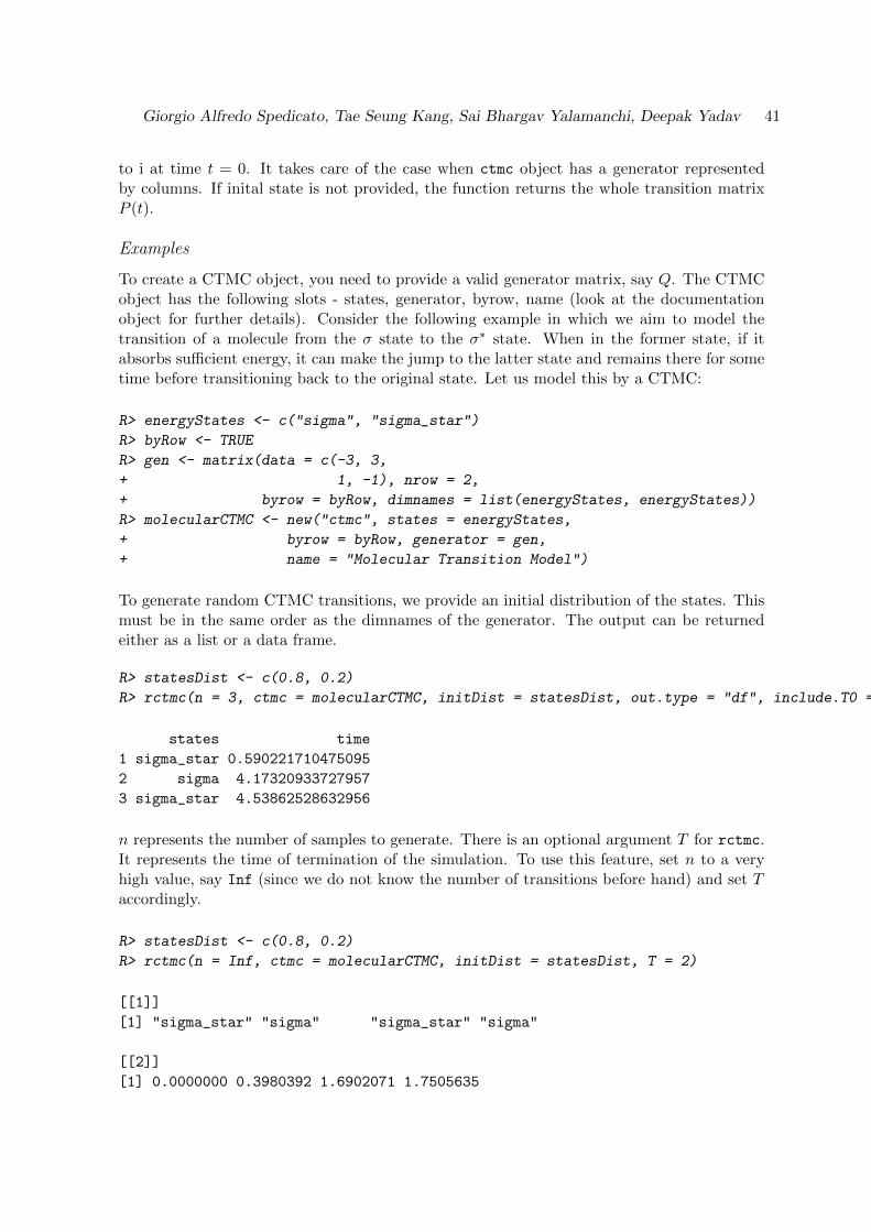
To create a CTMC object, you need to provide a valid generator matrix, say Q. The CTMCobject has the following slots - states, generator, byrow, name (look at the documentationobject for further details). Consider the following example in which we aim to model thetransition of a molecule from the σ state to the σ∗ state. When in the former state, if itabsorbs sufficient energy, it can make the jump to the latter state and remains there for sometime before transitioning back to the original state. Let us model this by a CTMC:
R> energyStates <- c("sigma", "sigma_star")
R> byRow <- TRUE
R> gen <- matrix(data = c(-3, 3,
+ 1, -1), nrow = 2,
+ byrow = byRow, dimnames = list(energyStates, energyStates))
R> molecularCTMC <- new("ctmc", states = energyStates,
+ byrow = byRow, generator = gen,
+ name = "Molecular Transition Model")
To generate random CTMC transitions, we provide an initial distribution of the states. Thismust be in the same order as the dimnames of the generator. The output can be returnedeither as a list or a data frame.
R> statesDist <- c(0.8, 0.2)
R> rctmc(n = 3, ctmc = molecularCTMC, initDist = statesDist, out.type = "df", include.T0 = FALSE)
states time
1 sigma_star 0.590221710475095
2 sigma 4.17320933727957
3 sigma_star 4.53862528632956
n represents the number of samples to generate. There is an optional argument T for rctmc.It represents the time of termination of the simulation. To use this feature, set n to a veryhigh value, say Inf (since we do not know the number of transitions before hand) and set Taccordingly.
R> statesDist <- c(0.8, 0.2)
R> rctmc(n = Inf, ctmc = molecularCTMC, initDist = statesDist, T = 2)
[[1]]
[1] "sigma_star" "sigma" "sigma_star" "sigma"
[[2]]
[1] 0.0000000 0.3980392 1.6902071 1.7505635
42 The markovchain package
To obtain the stationary distribution simply invoke the steadyStates function
R> steadyStates(molecularCTMC)
sigma sigma_star
[1,] 0.25 0.75
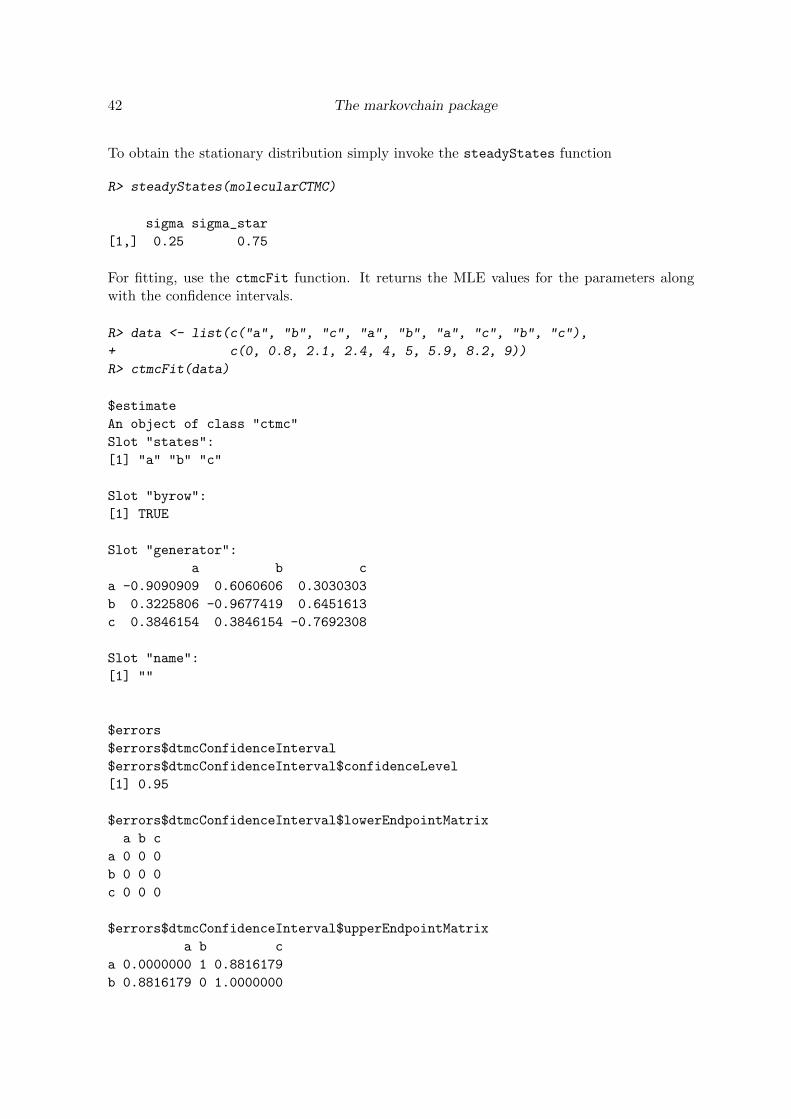
For fitting, use the ctmcFit function. It returns the MLE values for the parameters alongwith the confidence intervals.
R> data <- list(c("a", "b", "c", "a", "b", "a", "c", "b", "c"),
+ c(0, 0.8, 2.1, 2.4, 4, 5, 5.9, 8.2, 9))
R> ctmcFit(data)
$estimate
An object of class "ctmc"
Slot "states":
[1] "a" "b" "c"
Slot "byrow":
[1] TRUE
Slot "generator":
a b c
a -0.9090909 0.6060606 0.3030303
b 0.3225806 -0.9677419 0.6451613
c 0.3846154 0.3846154 -0.7692308
Slot "name":
[1] ""
$errors
$errors$dtmcConfidenceInterval
$errors$dtmcConfidenceInterval$confidenceLevel
[1] 0.95
$errors$dtmcConfidenceInterval$lowerEndpointMatrix
a b c
a 0 0 0
b 0 0 0
c 0 0 0
$errors$dtmcConfidenceInterval$upperEndpointMatrix
a b c
a 0.0000000 1 0.8816179
b 0.8816179 0 1.0000000
Giorgio Alfredo Spedicato, Tae Seung Kang, Sai Bhargav Yalamanchi, Deepak Yadav 43
c 1.0000000 1 0.0000000
$errors$lambdaConfidenceInterval
$errors$lambdaConfidenceInterval$lowerEndpointVector
[1] 0.04576665 0.04871934 0.00000000
$errors$lambdaConfidenceInterval$upperEndpointVector
[1] 1 1 1
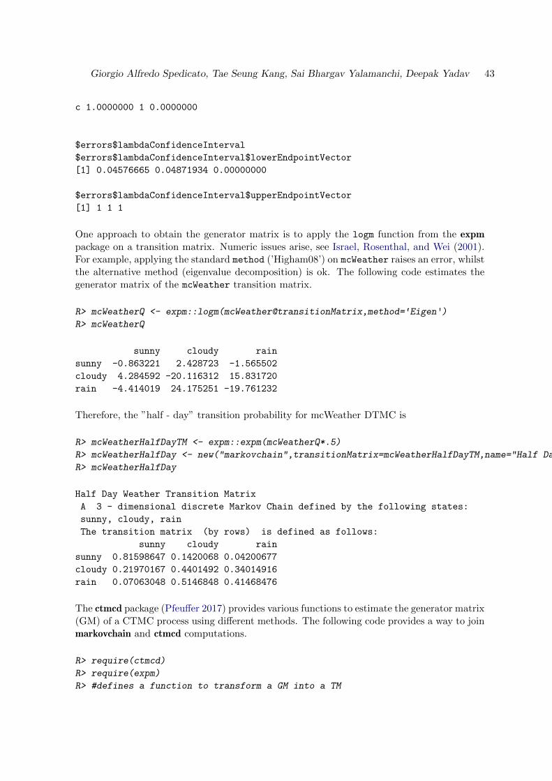
One approach to obtain the generator matrix is to apply the logm function from the expmpackage on a transition matrix. Numeric issues arise, see Israel, Rosenthal, and Wei (2001).For example, applying the standard method (’Higham08’) on mcWeather raises an error, whilstthe alternative method (eigenvalue decomposition) is ok. The following code estimates thegenerator matrix of the mcWeather transition matrix.
R> mcWeatherQ <- expm::logm(mcWeather@transitionMatrix,method='Eigen')
R> mcWeatherQ
sunny cloudy rain
sunny -0.863221 2.428723 -1.565502
cloudy 4.284592 -20.116312 15.831720
rain -4.414019 24.175251 -19.761232
Therefore, the ”half - day” transition probability for mcWeather DTMC is
R> mcWeatherHalfDayTM <- expm::expm(mcWeatherQ*.5)
R> mcWeatherHalfDay <- new("markovchain",transitionMatrix=mcWeatherHalfDayTM,name="Half Day Weather Transition Matrix")
R> mcWeatherHalfDay
Half Day Weather Transition Matrix
A 3 - dimensional discrete Markov Chain defined by the following states:
sunny, cloudy, rain
The transition matrix (by rows) is defined as follows:
sunny cloudy rain
sunny 0.81598647 0.1420068 0.04200677
cloudy 0.21970167 0.4401492 0.34014916
rain 0.07063048 0.5146848 0.41468476
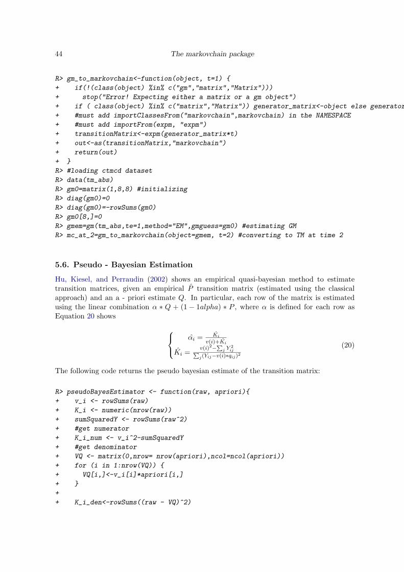
The ctmcd package (Pfeuffer 2017) provides various functions to estimate the generator matrix(GM) of a CTMC process using different methods. The following code provides a way to joinmarkovchain and ctmcd computations.
R> require(ctmcd)
R> require(expm)
R> #defines a function to transform a GM into a TM
44 The markovchain package
R> gm_to_markovchain<-function(object, t=1) {
+ if(!(class(object) %in% c("gm","matrix","Matrix")))
+ stop("Error! Expecting either a matrix or a gm object")
+ if ( class(object) %in% c("matrix","Matrix")) generator_matrix<-object else generator_matrix<-as.matrix(object[["par"]])
+ #must add importClassesFrom("markovchain",markovchain) in the NAMESPACE
+ #must add importFrom(expm, "expm")
+ transitionMatrix<-expm(generator_matrix*t)
+ out<-as(transitionMatrix,"markovchain")
+ return(out)
+ }
R> #loading ctmcd dataset
R> data(tm_abs)
R> gm0=matrix(1,8,8) #initializing
R> diag(gm0)=0
R> diag(gm0)=-rowSums(gm0)
R> gm0[8,]=0
R> gmem=gm(tm_abs,te=1,method="EM",gmguess=gm0) #estimating GM
R> mc_at_2=gm_to_markovchain(object=gmem, t=2) #converting to TM at time 2
5.6. Pseudo - Bayesian Estimation
Hu, Kiesel, and Perraudin (2002) shows an empirical quasi-bayesian method to estimatetransition matrices, given an empirical P transition matrix (estimated using the classicalapproach) and an a - priori estimate Q. In particular, each row of the matrix is estimatedusing the linear combination α ∗ Q + (1− 1alpha) ∗ P , where α is defined for each row asEquation 20 shows αi = Ki
v(i)+Ki
Ki =v(i)2−
∑j Y
2ij∑
j(Yij−v(i)∗qij)2(20)
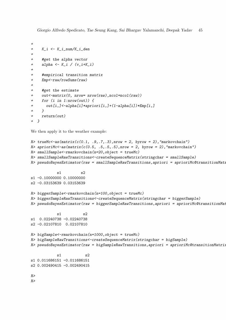
The following code returns the pseudo bayesian estimate of the transition matrix:
R> pseudoBayesEstimator <- function(raw, apriori){
+ v_i <- rowSums(raw)
+ K_i <- numeric(nrow(raw))
+ sumSquaredY <- rowSums(raw^2)
+ #get numerator
+ K_i_num <- v_i^2-sumSquaredY
+ #get denominator
+ VQ <- matrix(0,nrow= nrow(apriori),ncol=ncol(apriori))
+ for (i in 1:nrow(VQ)) {
+ VQ[i,]<-v_i[i]*apriori[i,]
+ }
+
+ K_i_den<-rowSums((raw - VQ)^2)
Giorgio Alfredo Spedicato, Tae Seung Kang, Sai Bhargav Yalamanchi, Deepak Yadav 45
+
+ K_i <- K_i_num/K_i_den
+
+ #get the alpha vector
+ alpha <- K_i / (v_i+K_i)
+
+ #empirical transition matrix
+ Emp<-raw/rowSums(raw)
+
+ #get the estimate
+ out<-matrix(0, nrow= nrow(raw),ncol=ncol(raw))
+ for (i in 1:nrow(out)) {
+ out[i,]<-alpha[i]*apriori[i,]+(1-alpha[i])*Emp[i,]
+ }
+ return(out)
+ }
We then apply it to the weather example:
R> trueMc<-as(matrix(c(0.1, .9,.7,.3),nrow = 2, byrow = 2),"markovchain")
R> aprioriMc<-as(matrix(c(0.5, .5,.5,.5),nrow = 2, byrow = 2),"markovchain")
R> smallSample<-rmarkovchain(n=20,object = trueMc)
R> smallSampleRawTransitions<-createSequenceMatrix(stringchar = smallSample)
R> pseudoBayesEstimator(raw = smallSampleRawTransitions,apriori = aprioriMc@transitionMatrix)-trueMc@transitionMatrix
s1 s2
s1 -0.10000000 0.10000000
s2 -0.03153639 0.03153639
R> biggerSample<-rmarkovchain(n=100,object = trueMc)
R> biggerSampleRawTransitions<-createSequenceMatrix(stringchar = biggerSample)
R> pseudoBayesEstimator(raw = biggerSampleRawTransitions,apriori = aprioriMc@transitionMatrix)-trueMc@transitionMatrix
s1 s2
s1 0.02240738 -0.02240738
s2 -0.02107810 0.02107810
R> bigSample<-rmarkovchain(n=1000,object = trueMc)
R> bigSampleRawTransitions<-createSequenceMatrix(stringchar = bigSample)
R> pseudoBayesEstimator(raw = bigSampleRawTransitions,apriori = aprioriMc@transitionMatrix)-trueMc@transitionMatrix
s1 s2
s1 0.011686151 -0.011686151
s2 0.002490415 -0.002490415
R>
R>
46 The markovchain package
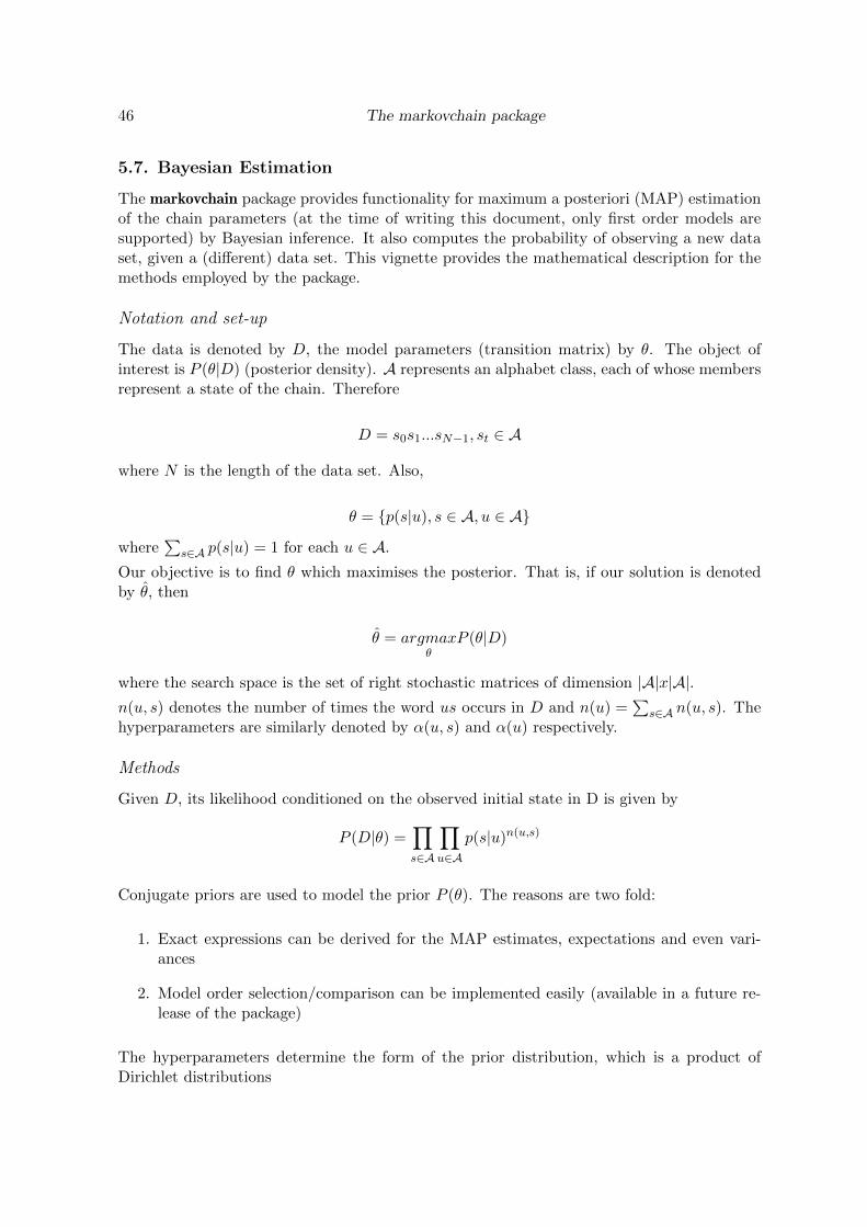
5.7. Bayesian Estimation
The markovchain package provides functionality for maximum a posteriori (MAP) estimationof the chain parameters (at the time of writing this document, only first order models aresupported) by Bayesian inference. It also computes the probability of observing a new dataset, given a (different) data set. This vignette provides the mathematical description for themethods employed by the package.
Notation and set-up
The data is denoted by D, the model parameters (transition matrix) by θ. The object ofinterest is P (θ|D) (posterior density). A represents an alphabet class, each of whose membersrepresent a state of the chain. Therefore
D = s0s1...sN−1, st ∈ A
where N is the length of the data set. Also,
θ = {p(s|u), s ∈ A, u ∈ A}
where∑
s∈A p(s|u) = 1 for each u ∈ A.
Our objective is to find θ which maximises the posterior. That is, if our solution is denotedby θ, then
θ = argmaxθ
P (θ|D)
where the search space is the set of right stochastic matrices of dimension |A|x|A|.n(u, s) denotes the number of times the word us occurs in D and n(u) =
∑s∈A n(u, s). The
hyperparameters are similarly denoted by α(u, s) and α(u) respectively.
Methods
Given D, its likelihood conditioned on the observed initial state in D is given by
P (D|θ) =∏s∈A
∏u∈A
p(s|u)n(u,s)
Conjugate priors are used to model the prior P (θ). The reasons are two fold:
1. Exact expressions can be derived for the MAP estimates, expectations and even vari-ances
2. Model order selection/comparison can be implemented easily (available in a future re-lease of the package)
The hyperparameters determine the form of the prior distribution, which is a product ofDirichlet distributions
Giorgio Alfredo Spedicato, Tae Seung Kang, Sai Bhargav Yalamanchi, Deepak Yadav 47
P (θ) =∏u∈A
{ Γ(α(u))∏s∈A Γ(α(u, s))
∏s∈A
p(s|u)α(u,s))−1}
where Γ(.) is the Gamma function. The hyperparameters are specified using the hyperparam
argument in the markovchainFit function. If this argument is not specified, then a defaultvalue of 1 is assigned to each hyperparameter resulting in the prior distribution of each chainparameter to be uniform over [0, 1].
Given the likelihood and the prior as described above, the evidence P (D) is simply given by
P (D) =
∫P (D|θ)P (θ)dθ
which simplifies to
P (D) =∏u∈A
{ Γ(α(u))∏s∈A Γ(α(u, s))
∏s∈A Γ(n(u, s) + α(u, s))
Γ(α(u) + n(u))
}Using Bayes’ theorem, the posterior now becomes (thanks to the choice of conjugate priors)
P (θ|D) =∏u∈A
{ Γ(n(u) + α(u))∏s∈A Γ(n(u, s) + α(u, s))
∏s∈A
p(s|u)n(u,s)+α(u,s))−1}
Since this is again a product of Dirichlet distributions, the marginalised distribution of aparticular parameter P (s|u) of our chain is given by
P (s|u) ∼ Beta(n(u, s) + α(u, s), n(u) + α(u)− n(u, s)− α(u, s))
Thus, the MAP estimate θ is given by
θ ={n(u, s) + α(u, s)− 1
n(u) + α(u)− |A|, s ∈ A, u ∈ A
}The function also returns the expected value, given by
Epostp(s|u) ={n(u, s) + α(u, s)
n(u) + α(u), s ∈ A, u ∈ A
}The variance is given by
Varpostp(s|u) =n(u, s) + α(u, s)
(n(u) + α(u))2n(u) + α(u)− n(u, s)− α(u, s)
n(u) + α(u) + 1
The square root of this quantity is the standard error, which is returned by the function.
The confidence intervals are constructed by computing the inverse of the beta integral.
Predictive distribution
Given the old data set, the probability of observing new data is P (D′|D) where D′ is the newdata set. Let m(u, s),m(u) denote the corresponding counts for the new data. Then,
P (D′|D) =
∫P (D′|θ)P (θ|D)dθ
48 The markovchain package
We already know the expressions for both quantities in the integral and it turns out to besimilar to evaluating the evidence
P (D′|D) =∏u∈A
{ Γ(α(u))∏s∈A Γ(α(u, s))
∏s∈A Γ(n(u, s) +m(u, s) + α(u, s))
Γ(α(u) + n(u) +m(u))
}
Choosing the hyperparameters
The hyperparameters model the shape of the parameters’ prior distribution. These mustbe provided by the user. The package offers functionality to translate a given prior belieftransition matrix into the hyperparameter matrix. It is assumed that this belief matrixcorresponds to the mean value of the parameters. Since the relation
Epriorp(s|u) =α(u, s)
α(u)
holds, the function accepts as input the belief matrix as well as a scaling vector (serves as aproxy for α(.)) and proceeds to compute α(., .).
Alternatively, the function accepts a data sample and infers the hyperparameters from it.Since the mode of a parameter (with respect to the prior distribution) is proportional to oneless than the corresponding hyperparameter, we set
α(u, s)− 1 = m(u, s)
where m(u, s) is the u− > s transition count in the data sample. This is regarded as a ’fakecount’ which helps α(u, s) to reflect knowledge of the data sample.
Usage and examples
R> weatherStates <- c("sunny", "cloudy", "rain")
R> byRow <- TRUE
R> weatherMatrix <- matrix(data = c(0.7, 0.2, 0.1,
+ 0.3, 0.4, 0.3,
+ 0.2, 0.4, 0.4),
+ byrow = byRow, nrow = 3,
+ dimnames = list(weatherStates, weatherStates))
R> mcWeather <- new("markovchain", states = weatherStates,
+ byrow = byRow, transitionMatrix = weatherMatrix,
+ name = "Weather")
R> weathersOfDays <- rmarkovchain(n = 365, object = mcWeather, t0 = "sunny")
For the purpose of this section, we shall continue to use the weather of days example intro-duced in the main vignette of the package (reproduced above for convenience).
Let us invoke the fit function to estimate the MAP parameters with 92% confidence boundsand hyperparameters as shown below, based on the first 200 days of the weather data. Ad-ditionally, let us find out what the probability is of observing the weather data for the next165 days. The usage would be as follows
Giorgio Alfredo Spedicato, Tae Seung Kang, Sai Bhargav Yalamanchi, Deepak Yadav 49
R> hyperMatrix<-matrix(c(1, 1, 2,
+ 3, 2, 1,
+ 2, 2, 3),
+ nrow = 3, byrow = TRUE,
+ dimnames = list(weatherStates,weatherStates))
R> markovchainFit(weathersOfDays[1:200], method = "map",
+ confidencelevel = 0.92, hyperparam = hyperMatrix)
$estimate
Bayesian Fit
A 3 - dimensional discrete Markov Chain defined by the following states:
cloudy, rain, sunny
The transition matrix (by rows) is defined as follows:
cloudy rain sunny
cloudy 0.3709677 0.2741935 0.3548387
rain 0.3809524 0.3809524 0.2380952
sunny 0.2135922 0.0776699 0.7087379
$expectedValue
cloudy rain sunny
cloudy 0.3692308 0.27692308 0.3538462
rain 0.3777778 0.37777778 0.2444444
sunny 0.2169811 0.08490566 0.6981132
$standardError
[,1] [,2] [,3]
[1,] 0.05940353 0.05508075 0.05885769
[2,] 0.07148453 0.07148453 0.06336426
[3,] 0.03984788 0.02694693 0.04438059
$confidenceInterval
$confidenceInterval$confidenceLevel
[1] 0.92
$confidenceInterval$lowerEndpointMatrix
[,1] [,2] [,3]
[1,] 0.2788643 0.1837403 0.2628715
[2,] 0.2728115 0.2728115 0.1312487
[3,] 0.1436350 0.0000000 0.6344429
$confidenceInterval$upperEndpointMatrix
[,1] [,2] [,3]
[1,] 0.4955338 0.3757588 0.4749592
[2,] 0.5431506 0.5431506 0.3509441
[3,] 0.2829567 0.1249744 1.0000000
50 The markovchain package
$logLikelihood
[1] -182.4175
R> predictiveDistribution(weathersOfDays[1:200],
+ weathersOfDays[201:365],hyperparam = hyperMatrix)
[1] -151.6332
The results should not change after permuting the dimensions of the matrix.
R> hyperMatrix2<- hyperMatrix[c(2,3,1), c(2,3,1)]
R> markovchainFit(weathersOfDays[1:200], method = "map",
+ confidencelevel = 0.92, hyperparam = hyperMatrix2)
$estimate
Bayesian Fit
A 3 - dimensional discrete Markov Chain defined by the following states:
cloudy, rain, sunny
The transition matrix (by rows) is defined as follows:
cloudy rain sunny
cloudy 0.3709677 0.2741935 0.3548387
rain 0.3809524 0.3809524 0.2380952
sunny 0.2135922 0.0776699 0.7087379
$expectedValue
cloudy rain sunny
cloudy 0.3692308 0.27692308 0.3538462
rain 0.3777778 0.37777778 0.2444444
sunny 0.2169811 0.08490566 0.6981132
$standardError
[,1] [,2] [,3]
[1,] 0.05940353 0.05508075 0.05885769
[2,] 0.07148453 0.07148453 0.06336426
[3,] 0.03984788 0.02694693 0.04438059
$confidenceInterval
$confidenceInterval$confidenceLevel
[1] 0.92
$confidenceInterval$lowerEndpointMatrix
[,1] [,2] [,3]
[1,] 0.2788643 0.1837403 0.2628715
[2,] 0.2728115 0.2728115 0.1312487
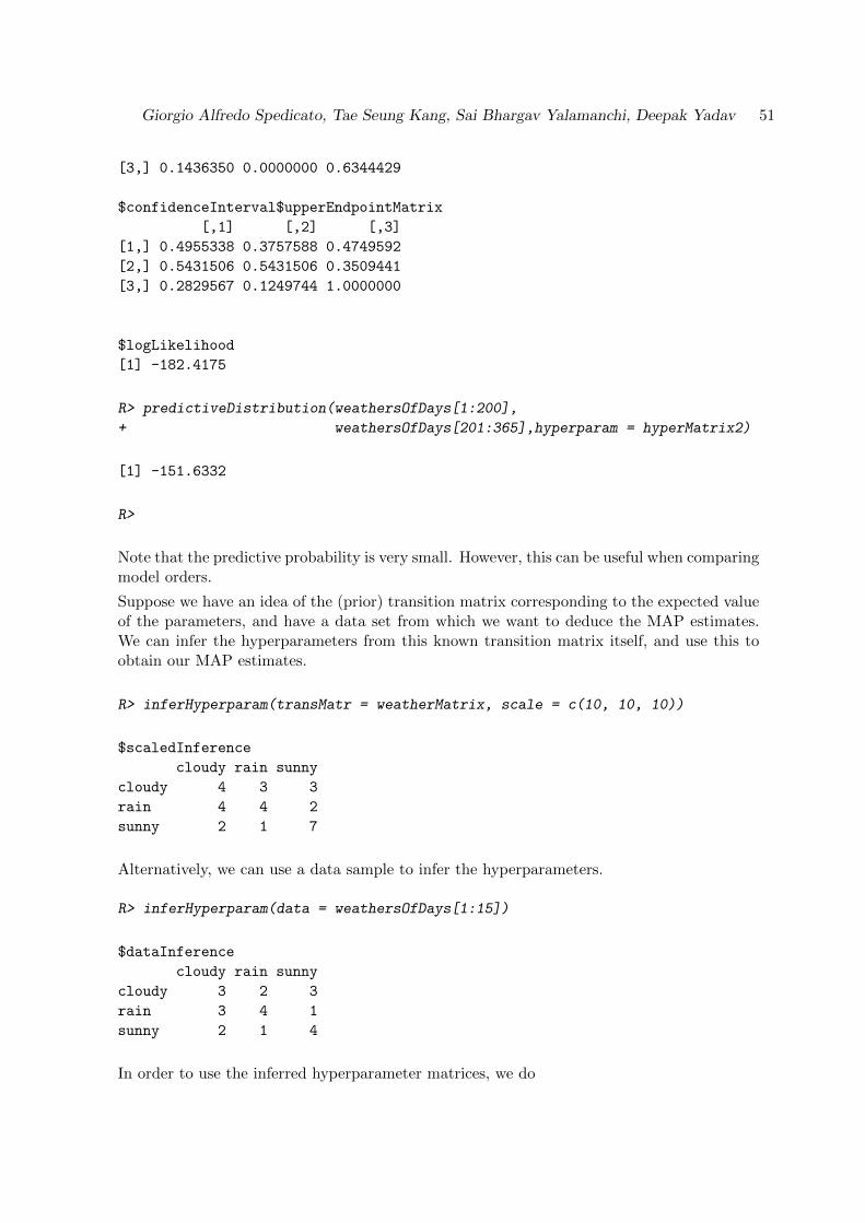
Giorgio Alfredo Spedicato, Tae Seung Kang, Sai Bhargav Yalamanchi, Deepak Yadav 51
[3,] 0.1436350 0.0000000 0.6344429
$confidenceInterval$upperEndpointMatrix
[,1] [,2] [,3]
[1,] 0.4955338 0.3757588 0.4749592
[2,] 0.5431506 0.5431506 0.3509441
[3,] 0.2829567 0.1249744 1.0000000
$logLikelihood
[1] -182.4175
R> predictiveDistribution(weathersOfDays[1:200],
+ weathersOfDays[201:365],hyperparam = hyperMatrix2)
[1] -151.6332
R>
Note that the predictive probability is very small. However, this can be useful when comparingmodel orders.
Suppose we have an idea of the (prior) transition matrix corresponding to the expected valueof the parameters, and have a data set from which we want to deduce the MAP estimates.We can infer the hyperparameters from this known transition matrix itself, and use this toobtain our MAP estimates.
R> inferHyperparam(transMatr = weatherMatrix, scale = c(10, 10, 10))
$scaledInference
cloudy rain sunny
cloudy 4 3 3
rain 4 4 2
sunny 2 1 7
Alternatively, we can use a data sample to infer the hyperparameters.
R> inferHyperparam(data = weathersOfDays[1:15])
$dataInference
cloudy rain sunny
cloudy 3 2 3
rain 3 4 1
sunny 2 1 4
In order to use the inferred hyperparameter matrices, we do
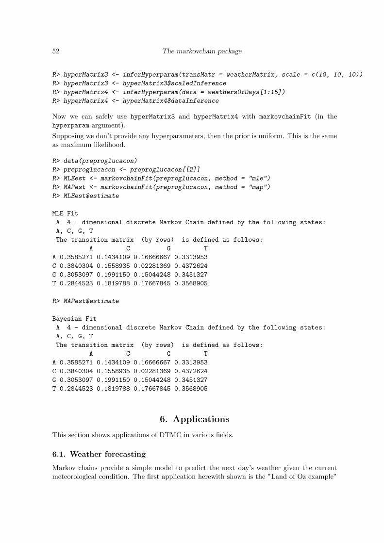
52 The markovchain package
R> hyperMatrix3 <- inferHyperparam(transMatr = weatherMatrix, scale = c(10, 10, 10))
R> hyperMatrix3 <- hyperMatrix3$scaledInference
R> hyperMatrix4 <- inferHyperparam(data = weathersOfDays[1:15])
R> hyperMatrix4 <- hyperMatrix4$dataInference
Now we can safely use hyperMatrix3 and hyperMatrix4 with markovchainFit (in thehyperparam argument).
Supposing we don’t provide any hyperparameters, then the prior is uniform. This is the sameas maximum likelihood.
R> data(preproglucacon)
R> preproglucacon <- preproglucacon[[2]]
R> MLEest <- markovchainFit(preproglucacon, method = "mle")
R> MAPest <- markovchainFit(preproglucacon, method = "map")
R> MLEest$estimate
MLE Fit
A 4 - dimensional discrete Markov Chain defined by the following states:
A, C, G, T
The transition matrix (by rows) is defined as follows:
A C G T
A 0.3585271 0.1434109 0.16666667 0.3313953
C 0.3840304 0.1558935 0.02281369 0.4372624
G 0.3053097 0.1991150 0.15044248 0.3451327
T 0.2844523 0.1819788 0.17667845 0.3568905
R> MAPest$estimate
Bayesian Fit
A 4 - dimensional discrete Markov Chain defined by the following states:
A, C, G, T
The transition matrix (by rows) is defined as follows:
A C G T
A 0.3585271 0.1434109 0.16666667 0.3313953
C 0.3840304 0.1558935 0.02281369 0.4372624
G 0.3053097 0.1991150 0.15044248 0.3451327
T 0.2844523 0.1819788 0.17667845 0.3568905
6. Applications
This section shows applications of DTMC in various fields.
6.1. Weather forecasting
Markov chains provide a simple model to predict the next day’s weather given the currentmeteorological condition. The first application herewith shown is the ”Land of Oz example”
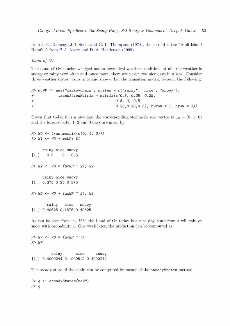
Giorgio Alfredo Spedicato, Tae Seung Kang, Sai Bhargav Yalamanchi, Deepak Yadav 53
from J. G. Kemeny, J. L.Snell, and G. L. Thompson (1974), the second is the ”Alofi IslandRainfall” from P. J. Avery and D. A. Henderson (1999).
Land of Oz
The Land of Oz is acknowledged not to have ideal weather conditions at all: the weather issnowy or rainy very often and, once more, there are never two nice days in a row. Considerthree weather states: rainy, nice and snowy. Let the transition matrix be as in the following:
R> mcWP <- new("markovchain", states = c("rainy", "nice", "snowy"),
+ transitionMatrix = matrix(c(0.5, 0.25, 0.25,
+ 0.5, 0, 0.5,
+ 0.25,0.25,0.5), byrow = T, nrow = 3))
Given that today it is a nice day, the corresponding stochastic row vector is w0 = (0 , 1 , 0)and the forecast after 1, 2 and 3 days are given by
R> W0 <- t(as.matrix(c(0, 1, 0)))
R> W1 <- W0 * mcWP; W1
rainy nice snowy
[1,] 0.5 0 0.5
R> W2 <- W0 * (mcWP ^ 2); W2
rainy nice snowy
[1,] 0.375 0.25 0.375
R> W3 <- W0 * (mcWP ^ 3); W3
rainy nice snowy
[1,] 0.40625 0.1875 0.40625
As can be seen from w1, if in the Land of Oz today is a nice day, tomorrow it will rain orsnow with probability 1. One week later, the prediction can be computed as
R> W7 <- W0 * (mcWP ^ 7)
R> W7
rainy nice snowy
[1,] 0.4000244 0.1999512 0.4000244
The steady state of the chain can be computed by means of the steadyStates method.
R> q <- steadyStates(mcWP)
R> q
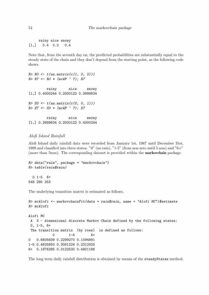
54 The markovchain package
rainy nice snowy
[1,] 0.4 0.2 0.4
Note that, from the seventh day on, the predicted probabilities are substantially equal to thesteady state of the chain and they don’t depend from the starting point, as the following codeshows.
R> R0 <- t(as.matrix(c(1, 0, 0)))
R> R7 <- R0 * (mcWP ^ 7); R7
rainy nice snowy
[1,] 0.4000244 0.2000122 0.3999634
R> S0 <- t(as.matrix(c(0, 0, 1)))
R> S7 <- S0 * (mcWP ^ 7); S7
rainy nice snowy
[1,] 0.3999634 0.2000122 0.4000244
Alofi Island Rainfall
Alofi Island daily rainfall data were recorded from January 1st, 1987 until December 31st,1989 and classified into three states: ”0” (no rain), ”1-5” (from non zero until 5 mm) and ”6+”(more than 5mm). The corresponding dataset is provided within the markovchain package.
R> data("rain", package = "markovchain")
R> table(rain$rain)
0 1-5 6+
548 295 253
The underlying transition matrix is estimated as follows.
R> mcAlofi <- markovchainFit(data = rain$rain, name = "Alofi MC")$estimate
R> mcAlofi
Alofi MC
A 3 - dimensional discrete Markov Chain defined by the following states:
0, 1-5, 6+
The transition matrix (by rows) is defined as follows:
0 1-5 6+
0 0.6605839 0.2299270 0.1094891
1-5 0.4625850 0.3061224 0.2312925
6+ 0.1976285 0.3122530 0.4901186
The long term daily rainfall distribution is obtained by means of the steadyStates method.
Giorgio Alfredo Spedicato, Tae Seung Kang, Sai Bhargav Yalamanchi, Deepak Yadav 55
R> steadyStates(mcAlofi)
0 1-5 6+
[1,] 0.5008871 0.2693656 0.2297473
6.2. Finance and Economics
Other relevant applications of DTMC can be found in Finance and Economics.
Finance
Credit ratings transitions have been successfully modelled with discrete time Markov chains.Some rating agencies publish transition matrices that show the empirical transition proba-bilities across credit ratings. The example that follows comes from CreditMetrics R package(Wittmann 2007), carrying Standard & Poor’s published data.
R> rc <- c("AAA", "AA", "A", "BBB", "BB", "B", "CCC", "D")
R> creditMatrix <- matrix(c(90.81, 8.33, 0.68, 0.06, 0.08, 0.02, 0.01, 0.01,
+ 0.70, 90.65, 7.79, 0.64, 0.06, 0.13, 0.02, 0.01,
+ 0.09, 2.27, 91.05, 5.52, 0.74, 0.26, 0.01, 0.06,
+ 0.02, 0.33, 5.95, 85.93, 5.30, 1.17, 1.12, 0.18,
+ 0.03, 0.14, 0.67, 7.73, 80.53, 8.84, 1.00, 1.06,
+ 0.01, 0.11, 0.24, 0.43, 6.48, 83.46, 4.07, 5.20,
+ 0.21, 0, 0.22, 1.30, 2.38, 11.24, 64.86, 19.79,
+ 0, 0, 0, 0, 0, 0, 0, 100
+ )/100, 8, 8, dimnames = list(rc, rc), byrow = TRUE)
It is easy to convert such matrices into markovchain objects and to perform some analyses
R> creditMc <- new("markovchain", transitionMatrix = creditMatrix,
+ name = "S&P Matrix")
R> absorbingStates(creditMc)
[1] "D"
Economics
For a recent application of markovchain in Economic, see Jacob (2014).
A dynamic system generates two kinds of economic effects (Bard 2000):
1. those incurred when the system is in a specified state, and
2. those incurred when the system makes a transition from one state to another.
Let the monetary amount of being in a particular state be represented as a m-dimensionalcolumn vector cS, while let the monetary amount of a transition be embodied in a CR matrix
56 The markovchain package
in which each component specifies the monetary amount of going from state i to state j in asingle step. Henceforth, Equation 21 represents the monetary of being in state i.
ci = cSi +
m∑j=1
CRijpij . (21)
Let c = [ci] and let ei be the vector valued 1 in the initial state and 0 in all other, then, if fn isthe random variable representing the economic return associated with the stochastic processat time n, Equation 22 holds:
E [fn (Xn) |X0 = i] = eiPnc. (22)
The following example assumes that a telephone company models the transition probabilitiesbetween customer/non-customer status by matrix P and the cost associated to states bymatrix M .
R> statesNames <- c("customer", "non customer")
R> P <- zeros(2); P[1, 1] <- .9; P[1, 2] <- .1; P[2, 2] <- .95; P[2, 1] <- .05;
R> rownames(P) <- statesNames; colnames(P) <- statesNames
R> mcP <- new("markovchain", transitionMatrix = P, name = "Telephone company")
R> M <- zeros(2); M[1, 1] <- -20; M[1, 2] <- -30; M[2, 1] <- -40; M[2, 2] <- 0
If the average revenue for existing customer is +100, the cost per state is computed as follows.
R> c1 <- 100 + conditionalDistribution(mcP, state = "customer") %*% M[1,]
R> c2 <- 0 + conditionalDistribution(mcP, state = "non customer") %*% M[2,]
For an existing customer, the expected gain (loss) at the fifth year is given by the followingcode.
R> as.numeric((c(1, 0)* mcP ^ 5) %*% (as.vector(c(c1, c2))))
[1] 48.96009
6.3. Actuarial science
Markov chains are widely applied in the field of actuarial science. Two classical applicationsare policyholders’ distribution across Bonus Malus classes in Motor Third Party Liability(MTPL) insurance (Section 6.3.1) and health insurance pricing and reserving (Section 6.3.2).
MPTL Bonus Malus
Bonus Malus (BM) contracts grant the policyholder a discount (enworsen) as a function ofthe number of claims in the experience period. The discount (enworsen) is applied on a pre-mium that already allows for known (a priori) policyholder characteristics (Denuit, Marechal,Pitrebois, and Walhin 2007) and it usually depends on vehicle, territory, the demographic
Giorgio Alfredo Spedicato, Tae Seung Kang, Sai Bhargav Yalamanchi, Deepak Yadav 57
profile of the policyholder, and policy coverages deep (deductible and policy limits).Since the proposed BM level depends on the claim on the previous period, it can be modelledby a discrete Markov chain. A very simplified example follows. Assume a BM scale from 1to 5, where 4 is the starting level. The evolution rules are shown in Equation 23:
bmt+1 = max (1, bmt − 1) ∗(N = 0
)+ min
(5, bmt + 2 ∗ N
)∗(N ≥ 1
). (23)
Tthe number of claim N is a random variable that is assumed to be Poisson distributed.
R> getBonusMalusMarkovChain <- function(lambda)
+ {
+ bmMatr <- zeros(5)
+ bmMatr[1, 1] <- dpois(x = 0, lambda)
+ bmMatr[1, 3] <- dpois(x = 1, lambda)
+ bmMatr[1, 5] <- 1 - ppois(q = 1, lambda)
+
+ bmMatr[2, 1] <- dpois(x = 0, lambda)
+ bmMatr[2, 4] <- dpois(x = 1, lambda)
+ bmMatr[2, 5] <- 1 - ppois(q = 1, lambda)
+
+ bmMatr[3, 2] <- dpois(x = 0, lambda)
+ bmMatr[3, 5] <- 1 - dpois(x=0, lambda)
+
+ bmMatr[4, 3] <- dpois(x = 0, lambda)
+ bmMatr[4, 5] <- 1 - dpois(x = 0, lambda)
+
+ bmMatr[5, 4] <- dpois(x = 0, lambda)
+ bmMatr[5, 5] <- 1 - dpois(x = 0, lambda)
+ stateNames <- as.character(1:5)
+ out <- new("markovchain", transitionMatrix = bmMatr,
+ states = stateNames, name = "BM Matrix")
+ return(out)
+ }
R>
Assuming that the a-priori claim frequency per car-year is 0.05 in the class (being the classthe group of policyholders that share the same common characteristics), the underlying BMtransition matrix and its underlying steady state are as follows.
R> bmMc <- getBonusMalusMarkovChain(0.05)
R> as.numeric(steadyStates(bmMc))
[1] 0.895836079 0.045930498 0.048285405 0.005969247 0.003978772
If the underlying BM coefficients of the class are 0.5, 0.7, 0.9, 1.0, 1.25, this means that theaverage BM coefficient applied on the long run to the class is given by
58 The markovchain package
R> sum(as.numeric(steadyStates(bmMc)) * c(0.5, 0.7, 0.9, 1, 1.25))
[1] 0.534469
This means that the average premium paid by policyholders in the portfolio almost halves inthe long run.
Health insurance example
Actuaries quantify the risk inherent in insurance contracts evaluating the premium of insur-ance contract to be sold (therefore covering future risk) and evaluating the actuarial reservesof existing portfolios (the liabilities in terms of benefits or claims payments due to policyholderarising from previously sold contracts), see Deshmukh (2012) for details.
An applied example can be performed using the data from De Angelis, Paolo and Di Falco,L. (2016) that has been saved in the exdata folder.
R> ltcDemoPath<-system.file("extdata", "ltdItaData.txt", package = "markovchain")
R> ltcDemo<-read.table(file = ltcDemoPath, header=TRUE, sep=";",dec = ".")
R> head(ltcDemo)
age pAD pID pAI pAA
1 20 0.0004616002 0.01083364 0.0001762467 0.9993622
2 21 0.0004824888 0.01079719 0.0001710577 0.9993465
3 22 0.0004949938 0.01177076 0.0001592333 0.9993458
4 23 0.0005042935 0.01159394 0.0001605731 0.9993351
5 24 0.0005074193 0.01260574 0.0001606504 0.9993319
6 25 0.0005154267 0.01526364 0.0001643603 0.9993202
The data shows the probability of transition between the state of (A)ctive, to (I)ll and Dead.It is easy to complete the transition matrix.
R> ltcDemo<-transform(ltcDemo,
+ pIA=0,
+ pII=1-pID,
+ pDD=1,
+ pDA=0,
+ pDI=0)
Now we build a function that returns the transition during the t+ 1 th year, assuming thatthe subject has attained year t.
R> possibleStates<-c("A","I","D")
R> getMc4Age<-function(age) {
+ transitionsAtAge<-ltcDemo[ltcDemo$age==age,]
+
+ myTransMatr<-matrix(0, nrow=3,ncol = 3,dimnames = list(possibleStates,possibleStates))
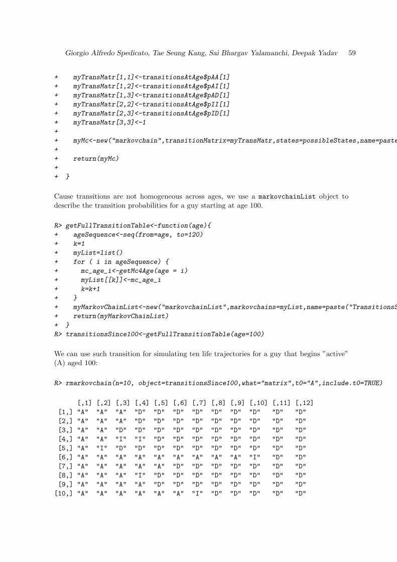
Giorgio Alfredo Spedicato, Tae Seung Kang, Sai Bhargav Yalamanchi, Deepak Yadav 59
+ myTransMatr[1,1]<-transitionsAtAge$pAA[1]
+ myTransMatr[1,2]<-transitionsAtAge$pAI[1]
+ myTransMatr[1,3]<-transitionsAtAge$pAD[1]
+ myTransMatr[2,2]<-transitionsAtAge$pII[1]
+ myTransMatr[2,3]<-transitionsAtAge$pID[1]
+ myTransMatr[3,3]<-1
+
+ myMc<-new("markovchain",transitionMatrix=myTransMatr,states=possibleStates,name=paste("Age",age,"transition matrix"))
+
+ return(myMc)
+
+ }
Cause transitions are not homogeneous across ages, we use a markovchainList object todescribe the transition probabilities for a guy starting at age 100.
R> getFullTransitionTable<-function(age){
+ ageSequence<-seq(from=age, to=120)
+ k=1
+ myList=list()
+ for ( i in ageSequence) {
+ mc_age_i<-getMc4Age(age = i)
+ myList[[k]]<-mc_age_i
+ k=k+1
+ }
+ myMarkovChainList<-new("markovchainList",markovchains=myList,name=paste("TransitionsSinceAge",age,sep=""))
+ return(myMarkovChainList)
+ }
R> transitionsSince100<-getFullTransitionTable(age=100)
We can use such transition for simulating ten life trajectories for a guy that begins ”active”(A) aged 100:
R> rmarkovchain(n=10, object=transitionsSince100,what="matrix",t0="A",include.t0=TRUE)
[,1] [,2] [,3] [,4] [,5] [,6] [,7] [,8] [,9] [,10] [,11] [,12]
[1,] "A" "A" "A" "D" "D" "D" "D" "D" "D" "D" "D" "D"
[2,] "A" "A" "A" "D" "D" "D" "D" "D" "D" "D" "D" "D"
[3,] "A" "A" "D" "D" "D" "D" "D" "D" "D" "D" "D" "D"
[4,] "A" "A" "I" "I" "D" "D" "D" "D" "D" "D" "D" "D"
[5,] "A" "I" "D" "D" "D" "D" "D" "D" "D" "D" "D" "D"
[6,] "A" "A" "A" "A" "A" "A" "A" "A" "A" "I" "D" "D"
[7,] "A" "A" "A" "A" "A" "D" "D" "D" "D" "D" "D" "D"
[8,] "A" "A" "A" "I" "D" "D" "D" "D" "D" "D" "D" "D"
[9,] "A" "A" "A" "A" "D" "D" "D" "D" "D" "D" "D" "D"
[10,] "A" "A" "A" "A" "A" "A" "I" "D" "D" "D" "D" "D"

60 The markovchain package
[,13] [,14] [,15] [,16] [,17] [,18] [,19] [,20] [,21] [,22]
[1,] "D" "D" "D" "D" "D" "D" "D" "D" "D" "D"
[2,] "D" "D" "D" "D" "D" "D" "D" "D" "D" "D"
[3,] "D" "D" "D" "D" "D" "D" "D" "D" "D" "D"
[4,] "D" "D" "D" "D" "D" "D" "D" "D" "D" "D"
[5,] "D" "D" "D" "D" "D" "D" "D" "D" "D" "D"
[6,] "D" "D" "D" "D" "D" "D" "D" "D" "D" "D"
[7,] "D" "D" "D" "D" "D" "D" "D" "D" "D" "D"
[8,] "D" "D" "D" "D" "D" "D" "D" "D" "D" "D"
[9,] "D" "D" "D" "D" "D" "D" "D" "D" "D" "D"
[10,] "D" "D" "D" "D" "D" "D" "D" "D" "D" "D"
Lets consider 1000 simulated live trajectories, for a healty guy aged 80. We can compute theexpected time a guy will be disabled starting active at age 100.
R> transitionsSince80<-getFullTransitionTable(age=80)
R> lifeTrajectories<-rmarkovchain(n=1e3, object=transitionsSince80,what="matrix",t0="A",include.t0=TRUE)
R> temp<-matrix(0,nrow=nrow(lifeTrajectories),ncol = ncol(lifeTrajectories))
R> temp[lifeTrajectories=="I"]<-1
R> expected_period_disabled<-mean(rowSums((temp)))
R> expected_period_disabled
[1] 1.361
Assuming that the health insurance will pay a benefit of 12000 per year disabled and thatthe real interest rate is 0.02, we can compute the lump sum premium at 80.
R> mean(rowMeans(12000*temp%*%( matrix((1+0.02)^-seq(from=0, to=ncol(temp)-1)))))
[1] 13621.67
6.4. Sociology
Markov chains have been actively used to model progressions and regressions between socialclasses. The first study was performed by Glass and Hall (1954), while a more recent ap-plication can be found in Jo Blanden and Machin (2005). The table that follows shows theincome quartile of the father when the son was 16 (in 1984) and the income quartile of theson when aged 30 (in 2000) for the 1970 cohort.
R> data("blanden")
R> mobilityMc <- as(blanden, "markovchain")
R> mobilityMc
Unnamed Markov chain
A 4 - dimensional discrete Markov Chain defined by the following states:
Bottom, 2nd, 3rd, Top
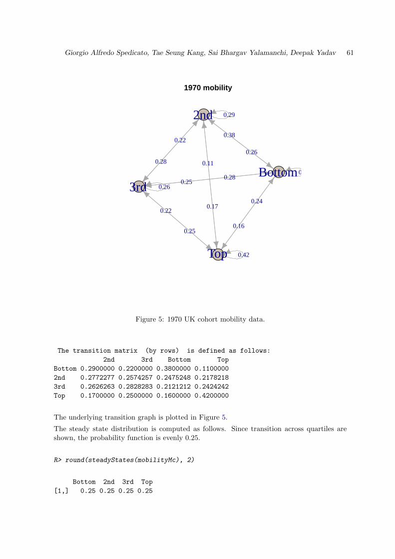
Giorgio Alfredo Spedicato, Tae Seung Kang, Sai Bhargav Yalamanchi, Deepak Yadav 61
1970 mobility
0.29
0.26
0.21
0.42
0.220.38
0.110.28
0.25
0.22
0.26
0.28
0.240.17
0.250.16
●
●●
●
2nd
3rdBottom
Top
Figure 5: 1970 UK cohort mobility data.
The transition matrix (by rows) is defined as follows:
2nd 3rd Bottom Top
Bottom 0.2900000 0.2200000 0.3800000 0.1100000
2nd 0.2772277 0.2574257 0.2475248 0.2178218
3rd 0.2626263 0.2828283 0.2121212 0.2424242
Top 0.1700000 0.2500000 0.1600000 0.4200000
The underlying transition graph is plotted in Figure 5.
The steady state distribution is computed as follows. Since transition across quartiles areshown, the probability function is evenly 0.25.
R> round(steadyStates(mobilityMc), 2)
Bottom 2nd 3rd Top
[1,] 0.25 0.25 0.25 0.25
62 The markovchain package
6.5. Genetics and Medicine
This section contains two examples: the first shows the use of Markov chain models in genetics,the second shows an application of Markov chains in modelling diseases’ dynamics.
Genetics
P. J. Avery and D. A. Henderson (1999) discusses the use of Markov chains in model Preprogu-cacon gene protein bases sequence. The preproglucacon dataset in markovchain containsthe dataset shown in the package.
R> data("preproglucacon", package = "markovchain")
It is possible to model the transition probabilities between bases as shown in the followingcode.
R> mcProtein <- markovchainFit(preproglucacon$preproglucacon,
+ name = "Preproglucacon MC")$estimate
R> mcProtein
Preproglucacon MC
A 4 - dimensional discrete Markov Chain defined by the following states:
A, C, G, T
The transition matrix (by rows) is defined as follows:
A C G T
A 0.3585271 0.1434109 0.16666667 0.3313953
C 0.3840304 0.1558935 0.02281369 0.4372624
G 0.3053097 0.1991150 0.15044248 0.3451327
T 0.2844523 0.1819788 0.17667845 0.3568905
Medicine
Discrete-time Markov chains are also employed to study the progression of chronic diseases.The following example is taken from B. A. Craig and A. A. Sendi (2002). Starting from sixmonth follow-up data, the maximum likelihood estimation of the monthly transition matrix isobtained. This transition matrix aims to describe the monthly progression of CD4-cell countsof HIV infected subjects.
R> craigSendiMatr <- matrix(c(682, 33, 25,
+ 154, 64, 47,
+ 19, 19, 43), byrow = T, nrow = 3)
R> hivStates <- c("0-49", "50-74", "75-UP")
R> rownames(craigSendiMatr) <- hivStates
R> colnames(craigSendiMatr) <- hivStates
R> craigSendiTable <- as.table(craigSendiMatr)
R> mcM6 <- as(craigSendiTable, "markovchain")
R> mcM6@name <- "Zero-Six month CD4 cells transition"
R> mcM6
Giorgio Alfredo Spedicato, Tae Seung Kang, Sai Bhargav Yalamanchi, Deepak Yadav 63
Zero-Six month CD4 cells transition
A 3 - dimensional discrete Markov Chain defined by the following states:
0-49, 50-74, 75-UP
The transition matrix (by rows) is defined as follows:
0-49 50-74 75-UP
0-49 0.9216216 0.04459459 0.03378378
50-74 0.5811321 0.24150943 0.17735849
75-UP 0.2345679 0.23456790 0.53086420
As shown in the paper, the second passage consists in the decomposition of M6 = V ·D ·V −1in order to obtain M1 as M1 = V ·D1/6 · V −1 .
R> eig <- eigen(mcM6@transitionMatrix)
R> D <- diag(eig$values)
R> V <- eig$vectors
R> V %*% D %*% solve(V)
[,1] [,2] [,3]
[1,] 0.9216216 0.04459459 0.03378378
[2,] 0.5811321 0.24150943 0.17735849
[3,] 0.2345679 0.23456790 0.53086420
R> d <- D ^ (1/6)
R> M <- V %*% d %*% solve(V)
R> mcM1 <- new("markovchain", transitionMatrix = M, states = hivStates)
7. Discussion, issues and future plans
The markovchain package has been designed in order to provide easily handling of DTMCand communication with alternative packages.
Some numerical issues have been found when working with matrix algebra using R internallinear algebra kernel (the same calculations performed with MATLAB gave a more accurateresult). Some temporary workarounds have been implemented. For example, the conditionfor row/column sums to be equal to one is valid up to fifth decimal. Similarly, when extractingthe eigenvectors only the real part is taken.
Such limitations are expected to be overcome in future releases. Similarly, future versions ofthe package are expected to improve the code in terms of numerical accuracy and rapidity.An intitial rewriting of internal function in C++ by means of Rcpp package (Eddelbuettel2013) has been started.
Aknowledgments
The package was selected for Google Summer of Code 2015 support. The authors wish tothank Michael Cole, Tobi Gutman and Mildenberger Thoralf for their suggestions and bug
64 The markovchain package
checks. A final thanks also to Dr. Simona C. Minotti and Dr. Mirko Signorelli for theirsupport in drafting this version of the vignettes.
References
Allaire J, Francois R, Ushey K, Vandenbrouck G, Geelnard M, Intel (2016). RcppParallel:Parallel Programming Tools for ’Rcpp’. R package version 4.3.19, URL http://rcppcore.
github.io/RcppParallel/.
Anderson TW, Goodman LA (1957). “Statistical inference about Markov chains.” The Annalsof Mathematical Statistics, pp. 89–110.
B A Craig, A A Sendi (2002). “Estimation of the Transition Matrix of a Discrete-TimeMarkov Chain.” Health Economics, 11, 33–42.
Bard JF (2000). “Lecture 12.5 - Additional Issues Concerning Discrete-TimeMarkov Chains.” URL http://www.me.utexas.edu/~jensen%20/ORMM/instruction/
powerpoint/or_models_09/12.5_dtmc2.ppt.
Bremaud P (1999). “Discrete-Time Markov Models.” In Markov Chains, pp. 53–93. Springer.
Chambers J (2008). Software for Data Analysis: Programming with R. Statistics and com-puting. Springer-Verlag. ISBN 9780387759357.
Ching WK, Ng MK, Fung ES (2008). “Higher-order multivariate Markov chains and theirapplications.” Linear Algebra and its Applications, 428(2), 492–507.
Csardi G, Nepusz T (2006). “The igraph Software Package for Complex Network Research.”InterJournal, Complex Systems, 1695. URL http://igraph.sf.net.
De Angelis, Paolo, Di Falco, L (2016). Assicurazioni sulla salute: caratteristiche, modelliattuariali e basi tecniche. Il Mulino. Il Mulino. ISBN 9788815260840. URL https://
books.google.it/books?id=D56bjgEACAAJ.
de Wreede LC, Fiocco M, Putter H (2011). “mstate: An R Package for the Analysis ofCompeting Risks and Multi-State Models.” Journal of Statistical Software, 38(7), 1–30.URL http://www.jstatsoft.org/v38/i07/.
Denuit M, Marechal X, Pitrebois S, Walhin JF (2007). Actuarial modelling of claim counts:Risk classification, credibility and bonus-malus systems. Wiley.
Deshmukh S (2012). Multiple Decrement Models in Insurance: An Introduction Using R.SpringerLink : Bucher. Springer-Verlag. ISBN 9788132206590.
Dobrow RP (2016). Introduction to Stochastic Processes with R. John Wiley & Sons.
Eddelbuettel D (2013). Seamless R and C++ Integration with Rcpp. Springer-Verlag, NewYork. ISBN 978-1-4614-6867-7.
Feres R (2007). “Notes for Math 450 MATLAB Listings for Markov Chains.” URL http:
//www.math.wustl.edu/~feres/Math450Lect04.pdf.
Giorgio Alfredo Spedicato, Tae Seung Kang, Sai Bhargav Yalamanchi, Deepak Yadav 65
Geyer CJ, Johnson LT (2013). mcmc: Markov Chain Monte Carlo. R package version 0.9-2,URL http://CRAN.R-project.org/package=mcmc.
Glass D, Hall JR (1954). “Social Mobility in Great Britain: A Study in IntergenerationalChange in Status.” In Social Mobility in Great Britain. Routledge and Kegan Paul.
Goulet V, Dutang C, Maechler M, Firth D, Shapira M, Stadelmann M, expm-developers@listsR-forgeR-projectorg (2013). expm: Matrix Exponential. R package version0.99-1, URL http://CRAN.R-project.org/package=expm.
Himmelmann SSDDL, wwwlinhicom (2010). HMM: HMM - Hidden Markov Models. Rpackage version 1.0, URL http://CRAN.R-project.org/package=HMM.
Hu YT, Kiesel R, Perraudin W (2002). “The estimation of transition matrices for sovereigncredit ratings.” Journal of Banking and Finance, 26(7), 1383–1406. ISSN 03784266. doi:10.1016/S0378-4266(02)00268-6.
Israel RB, Rosenthal JS, Wei JZ (2001). “Finding generators for Markov chains via empiricaltransition matrices, with applications to credit ratings.” Mathematical finance, 11(2), 245–265.
J G Kemeny, J LSnell, G L Thompson (1974). Introduction to Finite Mathematics. PrenticeHall.
Jackson CH (2011). “Multi-State Models for Panel Data: The msm Package for R.” Journalof Statistical Software, 38(8), 1–29. URL http://www.jstatsoft.org/v38/i08/.
Jacob I (2014). “Is R Cost Effective?” Electronic. Presented on Manchester R Meet-ing, URL http://www.rmanchester.org/Presentations/Ian%20Jacob%20-%20Is%20R%
20Cost%20Effective.pdf.
Jo Blanden PG, Machin S (2005). “Intergenerational Mobility in Europe and North America.”Technical report, Center for Economic Performances. URL http://cep.lse.ac.uk/about/
news/IntergenerationalMobility.pdf.
Konstantopoulos T (2009). “Markov Chains and Random Walks.” Lecture notes.
Kullback S, Kupperman M, Ku H (1962). “Tests for Contingency Tables and Marltov Chains.”Technometrics, 4(4), 573–608.
Montgomery J (2009). “Communication Classes.” URL http://www.ssc.wisc.edu/
~jmontgom/commclasses.pdf.
Nicholson W (2013). DTMCPack: Suite of Functions Related to Discrete-Time Discrete-State Markov Chains. R package version 0.1-2, URL http://CRAN.R-project.org/
package=DTMCPack.
P J Avery, D A Henderson (1999). “Fitting Markov Chain Models to Discrete State Series.”Applied Statistics, 48(1), 53–61.
Pfeuffer M (2017). ctmcd: Estimating the Parameters of a Continuous-Time Markov Chainfrom Discrete-Time Data. R package version 1.1, URL https://CRAN.R-project.org/
package=ctmcd.
66 The markovchain package
R Core Team (2013). R: A Language and Environment for Statistical Computing. R Foun-dation for Statistical Computing, Vienna, Austria. URL http://www.R-project.org/.
Roebuck P (2011). matlab: MATLAB emulation package. R package version 0.8.9, URLhttp://CRAN.R-project.org/package=matlab.
Sison CP, Glaz J (1995). “Simultaneous confidence intervals and sample size determinationfor multinomial proportions.” Journal of the American Statistical Association, 90(429),366–369.
Skuriat-Olechnowska M (2005). Statistical inference and hypothesis testing for Markov chainswith Interval Censoring. diploma thesis, Delft University of Technology.
Snell L (1999). “Probability Book: chapter 11.” URL http://www.dartmouth.edu/~chance/
teaching_aids/books_articles/probability_book/Chapter11.pdf.
Spedicato GA (2017). “Discrete Time Markov Chains with R.” The R Journal. URL https:
//journal.r-project.org/archive/2017/RJ-2017-036/index.html.
Villacorta PJ (2012). MultinomialCI: Simultaneous confidence intervals for multinomialproportions according to the method by Sison and Glaz. R package version 1.0, URLhttp://CRAN.R-project.org/package=MultinomialCI.
Wittmann A (2007). CreditMetrics: Functions for Calculating the CreditMetrics Risk Model.R package version 0.0-2.
Wolfram Research I (2013a). URL http://www.wolfram.com/mathematica/new-in-9/
markov-chains-and-queues/structural-properties-of-finite-markov-processes.
html.
Wolfram Research I (2013b). Mathematica. Wolfram Research, Inc., ninth edition.
Affiliation:
Giorgio Alfredo SpedicatoPh.D C.Stat ACASUnipolSai R&DVia Firenze 11, Paderno Dugnano 20037 ItalyE-mail: [email protected]: www.statisticaladvisor.com
Tae Seung KangPh.D studentComputer & Information Science & EngineeringUniversity of FloridaGainesville, FL, USAE-mail: [email protected]
Giorgio Alfredo Spedicato, Tae Seung Kang, Sai Bhargav Yalamanchi, Deepak Yadav 67
Sai Bhargav YalamanchiB-Tech studentElectrical EngineeringIndian Institute of Technology, BombayMumbai - 400 076, IndiaE-mail: [email protected]
Deepak YadavB-Tech studentComputer Science and EngineeringIndian Institute of Technology, VaranasiUttar Pradesh - 221 005, IndiaE-mail: [email protected]