package ‘smm’ - the comprehensive r archive network ‘smm’ september 8, 2017 type package...
TRANSCRIPT

Package ‘SMM’September 8, 2017
Type Package
Title Simulation and Estimation of Multi-State Discrete-TimeSemi-Markov and Markov Models
Version 1.0.1
Date 2017-09-08
Depends seqinr, DiscreteWeibull
AuthorVlad Stefan Barbu, Caroline Berard, Dominique Cellier, Mathilde Sautreuil and Nicolas Vergne
Maintainer Nicolas Vergne <[email protected]>
Description Performs parametric and non-parametric estimation and simulation for multi-state discrete-time semi-Markov processes.For the parametric estimation, several discrete distributions are considered for the so-journ times: Uniform, Geometric, Poisson, Discrete Weibull and Negative Binomial. The non-parametric estimation concerns the sojourn time distributions, where no assump-tions are done on the shape of distributions.Moreover, the estimation can be done on the basis of one or several sample paths, with or with-out censoring at the beginning or/and at the end of the sample paths. The implemented meth-ods are described in Barbu, V.S., Limnios, N. (2008) <doi:10.1007/978-0-387-73173-5>, Barbu, V.S., Limnios, N. (2008) <doi:10.1080/10485250701261913> andTrevezas, S., Limnios, N. (2011) <doi:10.1080/10485252.2011.555543>.Estimation and simulation of discrete-time k-th order Markov chains are also considered.
License GPL
VignetteBuilder utils
Suggests utils
NeedsCompilation no
Repository CRAN
Date/Publication 2017-09-08 12:50:13 UTC
R topics documented:SMM-package . . . . . . . . . . . . . . . . . . . . . . . . . . . . . . . . . . . . . . . . 2
1
2 SMM-package
AIC_Mk . . . . . . . . . . . . . . . . . . . . . . . . . . . . . . . . . . . . . . . . . . . 4AIC_SM . . . . . . . . . . . . . . . . . . . . . . . . . . . . . . . . . . . . . . . . . . . 6BIC_Mk . . . . . . . . . . . . . . . . . . . . . . . . . . . . . . . . . . . . . . . . . . . 8BIC_SM . . . . . . . . . . . . . . . . . . . . . . . . . . . . . . . . . . . . . . . . . . . 10estimMk . . . . . . . . . . . . . . . . . . . . . . . . . . . . . . . . . . . . . . . . . . . 12estimSM . . . . . . . . . . . . . . . . . . . . . . . . . . . . . . . . . . . . . . . . . . . 14InitialLawMk . . . . . . . . . . . . . . . . . . . . . . . . . . . . . . . . . . . . . . . . 23InitialLawSM . . . . . . . . . . . . . . . . . . . . . . . . . . . . . . . . . . . . . . . . 24LoglikelihoodMk . . . . . . . . . . . . . . . . . . . . . . . . . . . . . . . . . . . . . . 25LoglikelihoodSM . . . . . . . . . . . . . . . . . . . . . . . . . . . . . . . . . . . . . . 26simulMk . . . . . . . . . . . . . . . . . . . . . . . . . . . . . . . . . . . . . . . . . . . 29simulSM . . . . . . . . . . . . . . . . . . . . . . . . . . . . . . . . . . . . . . . . . . . 31
Index 37
SMM-package SMM : Semi-Markov and Markov Models
Description
This package performs parametric and non-parametric estimation and simulation for multi-statediscrete-time semi-Markov processes. For the parametric estimation, several discrete distributionsare considered for the sojourn times: Uniform, Geometric, Poisson, Discrete Weibull and Nega-tive Binomial. The non-parametric estimation concerns the sojourn time distributions, where noassumptions are done on the shape of distributions. Moreover, the estimation can be done on thebasis of one or several sample paths, with or without censoring at the beginning or/and at the endof the sample paths. Estimation and simulation of discrete-time k-th order Markov chains are alsoconsidered.
Details
This R package provides the following functions: estimSM, simulSM, LoglikelihoodSM, AIC_SM,BIC_SM, InitialLawSM, estimMk, simulMk, LoglikelihoodMK, AIC_Mk, BIC_Mk and InitialLawMk.
Author(s)
Vlad Stefan Barbu, [email protected] Berard, [email protected] Cellier, [email protected] Sautreuil, [email protected] Vergne, [email protected]
See Also
simulMk estimMk simulSM estimSM
SMM-package 3
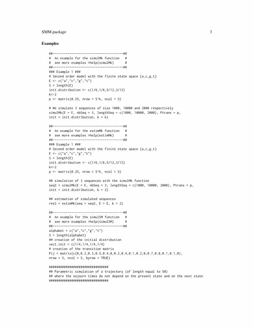
Examples
##--------------------------------------### An example for the simulMk function ## see more examples >help(simulMk) ###--------------------------------------##### Example 1 #### Second order model with the finite state space {a,c,g,t}E <- c("a","c","g","t")S = length(E)init.distribution <- c(1/6,1/6,5/12,3/12)k<-2p <- matrix(0.25, nrow = S^k, ncol = S)
# We simulate 3 sequences of size 1000, 10000 and 2000 respectivelysimulMk(E = E, nbSeq = 3, lengthSeq = c(1000, 10000, 2000), Ptrans = p,init = init.distribution, k = k)
##--------------------------------------### An example for the estimMk function ## see more examples >help(estimMk) ###--------------------------------------##### Example 1 #### Second order model with the finite state space {a,c,g,t}E <- c("a","c","g","t")S = length(E)init.distribution <- c(1/6,1/6,5/12,3/12)k<-2p <- matrix(0.25, nrow = S^k, ncol = S)
## simulation of 3 sequences with the simulMk functionseq3 = simulMk(E = E, nbSeq = 3, lengthSeq = c(1000, 10000, 2000), Ptrans = p,init = init.distribution, k = 2)
## estimation of simulated sequencesres3 = estimMk(seq = seq3, E = E, k = 2)
##--------------------------------------### An example for the simulSM function ## see more examples >help(simulSM) ###--------------------------------------##alphabet = c("a","c","g","t")S = length(alphabet)## creation of the initial distributionvect.init = c(1/4,1/4,1/4,1/4)# creation of the transition matrixPij = matrix(c(0,0.2,0.3,0.5,0.4,0,0.2,0.4,0.1,0.2,0,0.7,0.8,0.1,0.1,0),nrow = S, ncol = S, byrow = TRUE)
################################## Parametric simulation of a trajectory (of length equal to 50)## where the sojourn times do not depend on the present state and on the next state################################

4 AIC_Mk
## Simulation of a sequence of length 50seq50 = simulSM(E = alphabet, NbSeq = 1, lengthSeq = 50, TypeSojournTime = "f",
init = vect.init, Ptrans = Pij, distr = "pois", param = 2)
##--------------------------------------### An example for the simulSM function ## see more examples >help(simulSM) ###--------------------------------------##alphabet = c("a","c","g","t")S = length(alphabet)# creation of the transition matrixPij = matrix(c(0,0.2,0.3,0.5,0.4,0,0.2,0.4,0.1,0.2,0,0.7,0.8,0.1,0.1,0),nrow = S, ncol = S, byrow = TRUE)
Pij# [,1] [,2] [,3] [,4]#[1,] 0.0 0.2 0.3 0.5#[2,] 0.4 0.0 0.2 0.4#[3,] 0.1 0.2 0.0 0.7#[4,] 0.8 0.1 0.1 0.0
################################## Parametric estimation of a trajectory (of length equal to 5000)## where the sojourn times do not depend on the present state and on the next state################################## Simulation of a sequence of length 5000seq5000 = simulSM(E = alphabet, NbSeq = 1, lengthSeq = 5000, TypeSojournTime = "f",
init = c(1/4,1/4,1/4,1/4), Ptrans = Pij, distr = "pois", param = 2)
## Estimation of the simulated sequenceestSeq5000 = estimSM(seq = seq5000, E = alphabet, TypeSojournTime = "f",
distr = "pois", cens.end = 0, cens.beg = 0)
AIC_Mk AIC (Markov model)
Description
AIC
Usage
AIC_Mk(seq, E, mu, Ptrans, k)
Arguments
seq List of sequence(s)
E Vector of state space
AIC_Mk 5
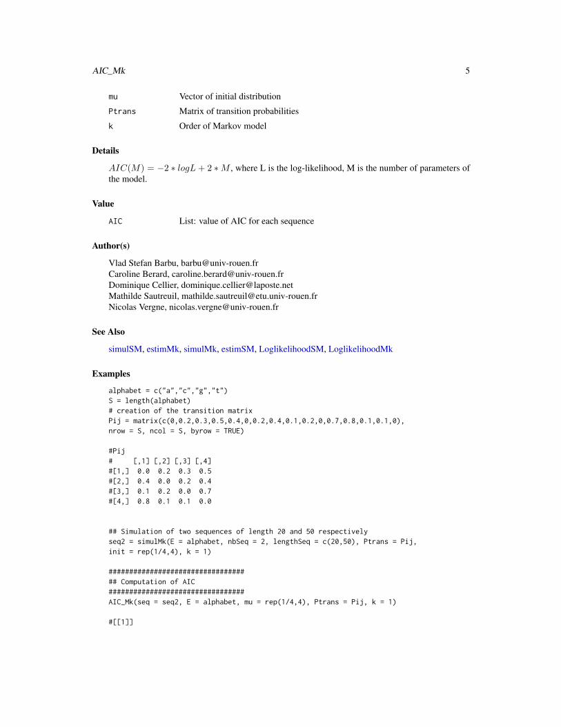
mu Vector of initial distribution
Ptrans Matrix of transition probabilities
k Order of Markov model
Details
AIC(M) = −2 ∗ logL + 2 ∗M , where L is the log-likelihood, M is the number of parameters ofthe model.
Value
AIC List: value of AIC for each sequence
Author(s)
Vlad Stefan Barbu, [email protected] Berard, [email protected] Cellier, [email protected] Sautreuil, [email protected] Vergne, [email protected]
See Also
simulSM, estimMk, simulMk, estimSM, LoglikelihoodSM, LoglikelihoodMk
Examples
alphabet = c("a","c","g","t")S = length(alphabet)# creation of the transition matrixPij = matrix(c(0,0.2,0.3,0.5,0.4,0,0.2,0.4,0.1,0.2,0,0.7,0.8,0.1,0.1,0),nrow = S, ncol = S, byrow = TRUE)
#Pij# [,1] [,2] [,3] [,4]#[1,] 0.0 0.2 0.3 0.5#[2,] 0.4 0.0 0.2 0.4#[3,] 0.1 0.2 0.0 0.7#[4,] 0.8 0.1 0.1 0.0
## Simulation of two sequences of length 20 and 50 respectivelyseq2 = simulMk(E = alphabet, nbSeq = 2, lengthSeq = c(20,50), Ptrans = Pij,init = rep(1/4,4), k = 1)
################################### Computation of AIC#################################AIC_Mk(seq = seq2, E = alphabet, mu = rep(1/4,4), Ptrans = Pij, k = 1)
#[[1]]

6 AIC_SM
#[1] 60.20263##[[2]]#[1] 115.7674
AIC_SM AIC (semi-Markov model)
Description
AIC
Usage
AIC_SM(seq, E, mu, Ptrans, distr = "NP", param = NULL, laws = NULL, TypeSojournTime)
Arguments
seq List of sequence(s)
E Vector of state space of length S
mu Vector of initial distribution
Ptrans Matrix of transition probabilities of the embedded Markov chain J = (Jm)m
distr - "NP" for nonparametric case, laws have to be used, param is useless- Matrix of distributions of size SxS if TypeSojournTime is equal to "fij";- Vector of distributions of size S if TypeSojournTime is equal to "fi" or "fj";- A distribution if TypeSojournTime is equal to "f".The distributions to be used in distr must be one of "uniform", "geom", "pois","dweibull", "nbinom".
param - Useless if distr = "NP"- Array of distribution parameters of size SxSx2 (2 corresponds to the maximalnumber of distribution parameters) if TypeSojournTime is equal to "fij";- Matrix of distribution parameters of size Sx2 if TypeSojournTime is equal to"fi" or "fj";- Vector of distribution parameters of length 2 if TypeSojournTime is equal to"f".
laws - Useless if distr 6= "NP"- Array of size SxSxKmax if TypeSojournTime is equal to "fij";- Matrix of size SxKmax if TypeSojournTime is equal to "fi" or "fj";- Vector of length Kmax if the TypeSojournTime is equal to "f".Kmax is the maximum length of the sojourn times.
TypeSojournTime
Character: "fij", "fi", "fj", "f"

AIC_SM 7
Details
AIC(M) = −2 ∗ logL + 2 ∗M , where L is the log-likelihood, M is the number of parameters ofthe model.
Value
AIC List: value of AIC for each sequence
Author(s)
Vlad Stefan Barbu, [email protected] Berard, [email protected] Cellier, [email protected] Sautreuil, [email protected] Vergne, [email protected]
See Also
simulSM, estimMk, simulMk, estimSM, LoglikelihoodSM, LoglikelihoodMk, AIC_Mk
Examples
alphabet = c("a","c","g","t")S = length(alphabet)## creation of the initial distributionvect.init = c(1/4,1/4,1/4,1/4)# creation of the transition matrixPij = matrix(c(0,0.2,0.3,0.5,0.4,0,0.2,0.4,0.1,0.2,0,0.7,0.8,0.1,0.1,0),nrow = S, ncol = S, byrow = TRUE)
#Pij# [,1] [,2] [,3] [,4]#[1,] 0.0 0.2 0.3 0.5#[2,] 0.4 0.0 0.2 0.4#[3,] 0.1 0.2 0.0 0.7#[4,] 0.8 0.1 0.1 0.0
################################## Parametric simulation of several trajectories (3 trajectories of length 1000, 10 000## and 2000 respectively)## with sojourn times depending on the present state and on the next state## the sojourn times are modelled by different distributions################################lengthSeq3 = c(1000, 10000, 2000)## creation of the distribution matrixdistr.matrix = matrix(c("dweibull", "pois", "geom", "nbinom", "geom", "nbinom","pois", "dweibull", "pois", "pois", "dweibull", "geom", "pois","geom", "geom","nbinom"), nrow = S, ncol = S, byrow = TRUE)## creation of an array containing the parametersparam1.matrix = matrix(c(0.6,2,0.4,4,0.7,2,5,0.6,2,3,0.6,0.6,4,0.3,0.4,4),

8 BIC_Mk
nrow = S, ncol = S, byrow = TRUE)param2.matrix = matrix(c(0.8,0,0,2,0,5,0,0.8,0,0,0.8,0,4,0,0,4),nrow = S, ncol = S, byrow = TRUE)param.array = array(c(param1.matrix, param2.matrix), c(S,S,2))### simulation of 3 sequencesseq3 = simulSM(E = alphabet, NbSeq = 3, lengthSeq = lengthSeq3,TypeSojournTime = "fij", init = vect.init, Ptrans = Pij, distr = distr.matrix,param = param.array, File.out = NULL)
################################### Computation of AIC#################################AIC_SM(seq = seq3, E = alphabet, mu = rep(1/4,4), Ptrans = Pij, distr = distr.matrix,
param = param.array, TypeSojournTime = "fij")
#[[1]]#[1] 1566.418##[[2]]#[1] 15683.48##[[3]]#[1] 3146.728
BIC_Mk BIC (Markov model)
Description
BIC
Usage
BIC_Mk(seq, E, mu, Ptrans, k)
Arguments
seq List of sequence(s)
E Vector of state space
mu Vector of initial distribution
Ptrans Matrix of transition probabilities
k Order of the Markov chain
Details
BIC(M) = −2∗ logL+ log(n)∗M , where L is the log-likelihood, M is the number of parametersof the model and n is the size of the sequence.

BIC_Mk 9
Value
BIC List: value of BIC for each sequence
Author(s)
Vlad Stefan Barbu, [email protected] Berard, [email protected] Cellier, [email protected] Sautreuil, [email protected] Vergne, [email protected]
See Also
simulSM, estimMk, simulMk, estimSM, LoglikelihoodSM, LoglikelihoodMk, AIC_Mk
Examples
alphabet = c("a","c","g","t")S = length(alphabet)# creation of the transition matrixPij = matrix(c(0,0.2,0.3,0.5,0.4,0,0.2,0.4,0.1,0.2,0,0.7,0.8,0.1,0.1,0),nrow = S, ncol = S, byrow = TRUE)
#Pij# [,1] [,2] [,3] [,4]#[1,] 0.0 0.2 0.3 0.5#[2,] 0.4 0.0 0.2 0.4#[3,] 0.1 0.2 0.0 0.7#[4,] 0.8 0.1 0.1 0.0
## Simulation of two sequences of length 20 and 50 respectivelyseq2 = simulMk(E = alphabet, nbSeq = 2, lengthSeq = c(20,50),Ptrans = Pij, init = rep(1/4,4), k = 1)
################################### Computation of BIC#################################BIC_Mk(seq = seq2, E = alphabet, mu = rep(1/4,4), Ptrans = Pij, k = 1)
#[[1]]#[1] 78.39401##[[2]]#[1] 133.7015

10 BIC_SM
BIC_SM BIC (semi-Markov model)
Description
BIC
Usage
BIC_SM(seq, E, mu, Ptrans, distr = "NP", param = NULL, laws = NULL, TypeSojournTime)
Arguments
seq List of sequence(s)
E Vector of state space
mu Vector of initial distribution
Ptrans Matrix of transition probabilities of the embedded Markov chain J = (Jm)m
distr - "NP" for nonparametric case, laws have to be used, param is useless- Matrix of distributions of size SxS if TypeSojournTime is equal to "fij";- Vector of distributions of size S if TypeSojournTime is equal to "fi" or "fj";- A distribution if TypeSojournTime is equal to "f".The distributions to be used in distr must be one of "uniform", "geom", "pois","dweibull", "nbinom".
param - Useless if distr = "NP"- Array of distribution parameters of size SxSx2 (2 corresponds to the maximalnumber of distribution parameters) if TypeSojournTime is equal to "fij";- Matrix of distribution parameters of size Sx2 if TypeSojournTime is equal to"fi" or "fj";- Vector of distribution parameters of length 2 if TypeSojournTime is equal to"f".
laws - Useless if distr 6= "NP"- Array of size SxSxKmax if TypeSojournTime is equal to "fij";- Matrix of size SxKmax if TypeSojournTime is equal to "fi" or "fj";- Vector of length Kmax if the TypeSojournTime is equal to "f".Kmax is the maximum length of the sojourn times.
TypeSojournTime
Character: "fij", "fi", "fj", "f"
Details
BIC(M) = −2∗ logL+ log(n)∗M , where L is the log-likelihood, M is the number of parametersof the model.

BIC_SM 11
Value
BIC List: value of BIC for each sequence
Author(s)
Vlad Stefan Barbu, [email protected] Berard, [email protected] Cellier, [email protected] Sautreuil, [email protected] Vergne, [email protected]
See Also
simulSM, estimMk, simulMk, estimSM, LoglikelihoodSM, LoglikelihoodMk, BIC_Mk, AIC_SM
Examples
alphabet = c("a","c","g","t")S = length(alphabet)## creation of the initial distributionvect.init = c(1/4,1/4,1/4,1/4)# creation of the transition matrixPij = matrix(c(0,0.2,0.3,0.5,0.4,0,0.2,0.4,0.1,0.2,0,0.7,0.8,0.1,0.1,0),nrow = S, ncol = S, byrow = TRUE)
#Pij# [,1] [,2] [,3] [,4]#[1,] 0.0 0.2 0.3 0.5#[2,] 0.4 0.0 0.2 0.4#[3,] 0.1 0.2 0.0 0.7#[4,] 0.8 0.1 0.1 0.0
################################## Parametric simulation of several trajectories (3 trajectories of length 1000, 10 000## and 2000 respectively)## where the sojourn time depend on the present state and the next state## the sojourn time is modelled by different distributions################################lengthSeq3 = c(1000, 10000, 2000)## creation of the distribution matrixdistr.matrix = matrix(c("dweibull", "pois", "geom", "nbinom", "geom", "nbinom","pois", "dweibull", "pois", "pois", "dweibull", "geom", "pois","geom", "geom","nbinom"), nrow = S, ncol = S, byrow = TRUE)
## creation of an array containing the parametersparam1.matrix = matrix(c(0.6,2,0.4,4,0.7,2,5,0.6,2,3,0.6,0.6,4,0.3,0.4,4),nrow = S, ncol = S, byrow = TRUE)
param2.matrix = matrix(c(0.8,0,0,2,0,5,0,0.8,0,0,0.8,0,4,0,0,4),nrow = S, ncol = S, byrow = TRUE)
param.array = array(c(param1.matrix, param2.matrix), c(S,S,2))## Simulation of 3 sequences

12 estimMk
seq3 = simulSM(E = alphabet, NbSeq = 3, lengthSeq = lengthSeq3,TypeSojournTime = "fij", init = vect.init, Ptrans = Pij, distr = distr.matrix,param = param.array, File.out = NULL)
################################### Computation of BIC#################################BIC_SM(seq = seq3, E = alphabet, mu = rep(1/4,4), Ptrans = Pij, distr = distr.matrix,
param = param.array, TypeSojournTime = "fij")
#[[1]]#[1] 1607.322##[[2]]#[1] 15846.36##[[3]]#[1] 3121.074
estimMk Estimation of a k-th order Markov chain
Description
Estimation of the transition matrix and initial law of a k-th order Markov chain starting from one orseveral sequences.
Usage
estimMk(file = NULL, seq, E, k)
estimMk(file, seq = NULL, E, k)
Arguments
file Path of the file in fasta format which contains the sequences from which toestimate
seq List of sequence(s)
E Vector of state space
k Order of the Markov chain
Details
Let X1, X2, ..., Xn be a trajectory of length n of the Markov chain X = (Xm)m∈N of order k=1with transition matrix Ptrans(i, j) = P (Xm+1 = j|Xm = i). The estimation of the transitionmatrix is ̂Ptrans(i, j) = Nij/Ni., where Nij is the number of transitions from state i to state j andNi. is the number of transition from state i to any state. For k > 1 we have similar expressions.

estimMk 13
The initial distribution of a k-th order Markov chain is defined as init = P (X1 = i). An estimationof the initial law for a first order Markov chain is assumed to be the estimation of the stationary law.If the order of the Markov is greater than 1, then an estimation of the initial law is init = Ni/N ,where Ni is the number occurences of state i in the sequences and N is the sum of the sequencelengths.
Value
estimMk returns the transition probability matrix of size (S^k)xS (with S = length(E)) and the initiallaw of size S estimated from the sequence(s) with a Markov model of order k.
The transition matrix is always given in the alphabetical and numerical order, even if the vector ofstate space is not given in this order.
Author(s)
Vlad Stefan Barbu, [email protected] Berard, [email protected] Cellier, [email protected] Sautreuil, [email protected] Vergne, [email protected]
See Also
simulMk, estimSM, simulSM
Examples
### Example 1 #### Second order model on the state space {a,c,g,t}E <- c("a","c","g","t")S = length(E)init.distribution <- c(1/6,1/6,5/12,3/12)k<-2p <- matrix(0.25, nrow = S^k, ncol = S)
## simulation of 3 sequences with the simulMk functionseq3 = simulMk(E = E, nbSeq = 3, lengthSeq = c(1000, 10000, 2000), Ptrans = p,init = init.distribution, k = 2)
## estimation of simulated sequencesres3 = estimMk(seq = seq3, E = E, k = 2)
## results of estimation# initial lawres3$init# [1] 0.2469048 0.2573333 0.2483810 0.2473810
# transition matrixres3$Ptrans# [,1] [,2] [,3] [,4]# [1,] 0.2690616 0.2338710 0.2602639 0.2368035

14 estimSM
# [2,] 0.2507553 0.2673716 0.2651057 0.2167674# [3,] 0.2517758 0.2533544 0.2588792 0.2367798# [4,] 0.2522376 0.2432872 0.2481692 0.2563059# [5,] 0.2501949 0.2595479 0.2595479 0.2307093# [6,] 0.2492775 0.2492775 0.2586705 0.2427746# [7,] 0.2337662 0.2792208 0.2438672 0.2445887# [8,] 0.2381306 0.2833828 0.2292285 0.2492582# [9,] 0.2462745 0.2627451 0.2384314 0.2525490#[10,] 0.2259760 0.2530030 0.2424925 0.2785285#[11,] 0.2469512 0.2423780 0.2599085 0.2507622#[12,] 0.2318393 0.2673879 0.2403400 0.2604328#[13,] 0.2866192 0.2668250 0.2185273 0.2280285#[14,] 0.2237711 0.2553191 0.2611886 0.2597212#[15,] 0.2465863 0.2465863 0.2441767 0.2626506#[16,] 0.2511346 0.2541604 0.2420575 0.2526475
### Example 2 ###E <- c(1,2,3)S <- length(E)init.distr <- rep(1/S, 3)p <- matrix(c(0.3,0.2,0.5,0.1,0.6,0.3,0.2,0.4,0.4), nrow = 3, byrow = TRUE)
## simulation with the simulMk functionseq1 = simulMk(E = E, nbSeq = 1, lengthSeq = 100, Ptrans = p, init = init.distr, k = 1)
## estimationres1 = estimMk(seq = seq1, E = E, k = 1)
## results of estimation# initial lawres1$init# [1] 0.1507212 0.4062408 0.4430380
# transition matrixres1$Ptrans# [,1] [,2] [,3]# [1,] 0.2500000 0.1875000 0.5625000# [2,] 0.0500000 0.5500000 0.4000000# [3,] 0.2093023 0.3488372 0.4418605
estimSM Estimation of a semi-Markov chain
Description
Estimation of a semi-Markov chain starting from one or several sequences. This estimation canbe parametric or non-parametric, non-censored, censored at the beginning and/or at the end of thesequence, with one or several trajectories. Several parametric distributions are considered (Uniform,Geometric, Poisson, Discrete Weibull and Negative Binomial).

estimSM 15
Usage
# parametric caseestimSM(file = NULL, seq, E, TypeSojournTime = "fij", distr, cens.end = 0,cens.beg = 0)
estimSM(file, seq = NULL, E, TypeSojournTime = "fij", distr, cens.end = 0,cens.beg = 0)
# non-parametric caseestimSM(file = NULL, seq, E, TypeSojournTime = "fij", distr = "NP", cens.end = 0,cens.beg = 0)
estimSM(file, seq = NULL, E, TypeSojournTime = "fij", distr = "NP", cens.end = 0,cens.beg = 0)
Arguments
file Path of the file in fasta format which contains the sequences from which toestimate
seq List of the sequence(s)
E Vector of state space of length STypeSojournTime
Character: "fij", "fi", "fj", "f" (for more explanations, see Details)
distr - "NP" for nonparametric case, laws have to be used, param is useless- Matrix of distributions of size SxS if TypeSojournTime is equal to "fij";- Vector of distributions of size S if TypeSojournTime is equal to "fi" or "fj";- A distribution if TypeSojournTime is equal to "f".The distributions to be used in distr must be one of "uniform", "geom", "pois","dweibull", "nbinom".
cens.beg Type of censoring at the beginning of sample paths; 1 (if the first sojourn timeis censored) or 0 (if not). All the sequences must be censored in the same way.
cens.end Type of censoring at the end of sample paths; 1 (if the last sojourn time is cen-sored) or 0 (if not). All the sequences must be censored in the same way.
Details
This function estimates a semi-Markov model in parametric and non-parametric case, taking intoaccount the type of sojourn time and the censoring described in references. The non-parametricestimation concerns sojourn time distributions defined by the user. For the parametric estimation,several discrete distributions are considered (see below).
The difference between the Markov model and the semi-Markov model concerns the modelisationof the sojourn time. With a Markov chain, the sojourn time distribution is modeled by a Geometricdistribution (in discrete time). With a semi-Markov chain, the sojourn time can be any arbitrarydistribution. In this package, the available distribution for a semi-Markov model are :
• Uniform: f(x) = 1/n for a ≤ x ≤ b, with n = b− a+ 1

16 estimSM
• Geometric: f(x) = θ(1 − θ)x for x = 0, 1, 2, . . . , n, 0 < θ ≤ 1, with n > 0 and θ is theprobability of success
• Poisson: f(x) = (λxexp(−λ))/x! for x = 0, 1, 2, . . . , n, with n > 0 and λ > 0
• Discrete Weibull of type 1: f(x) = q(x−1)β − qxβ
, x = 1, 2, 3, . . . , n, with n > 0, q is thefirst parameter and β is the second parameter
• Negative binomial: f(x) = Γ(x+α)/(Γ(α)x!)(α/(α+µ))α(µ/(α+µ))x, for x = 0, 1, 2, . . . , n,n > 0, Γ is the Gamma function, α is the parameter of overdispersion and µ is the mean
• Non-parametric
We define :
• the semi-Markov kernel qij(k) = P (Jm+1 = j, Tm+1 − Tm = k|Jm = i);• the transition matrix (Ptrans(i, j))i,j ∈ E of the embedded Markov chain J = (Jm)m,Ptrans(i, j) = P (Jm+1 = j|Jm = i);
• the initial distribution init = P (J1 = i) = P (Y1 = i);• the conditional sojourn time distributions (fij(k))i,j ∈ E, k ∈ N, fij(k) = P (Tm+1−Tm =k|Jm = i, Jm+1 = j), f is specified by the argument "param" in the parametric case and by"laws" in the non-parametric case.
The estimation of the transition matrix of the embedded Markov chain is ̂Ptrans(i, j) = Nij/Ni..
The estimation of the initial law is the limit law if the number of sequences is equal to 1, else theestimation of the inital law is init = N l
i/Nl, where N l
i is the number of times the state i appears inall the sequences and N l is the size of sequences.
In the parametric case, the distribution of sojourn time is calculated with the estimated parameters.
Note that qij(k) = Ptrans(i, j) ∗ fij(k) in the general case (depending on the present state andon the next state). For particular cases, we replace fij(k) by fi.(k) (depending on the present state"fi."), f.j(k) (depending on the next state "f.j") and f..(k) (depending neither on the present statenor on the next state "f").
In this package we can choose differents types of sojourn time. Four options are available for thesojourn times:
• depending on the present state and on the next state ("fij");• depending only on the present state ("fi");• depending only on the next state ("fj");• depending neither on the current, nor on the next state ("f").
If TypeSojournTime is equal to "fij", distr is a matrix (SxS) (e.g., if the row 1 of the 2nd column is"pois", that is to say we go from the first state to the second state following a Poisson distribution). IfTypeSojournTime is equal to "fi" or "fj", distr must be a vector (e.g., if the first element of vector is"geom", that is to say we go from the first state to any state according to a Geometric distribution).If TypeSojournTime is equal to "f", distr must be one of "uniform", "geom", "pois", "dweibull","nbinom" (e.g., if distr is equal to "nbinom", that is to say that the sojourn times when going fromany state to any state follows a Negative Binomial distribution). For the non-parametric case, distris equal to "NP" whatever type of sojourn time given.
If the sequence is censored at the beginning and at the end, cens.beg must be equal to 1 and cens.endmust be equal to 1 too. All the sequences must be censored in the same way.
At any use of the function, a file in .txt format is created. This file contains the output of the function.
estimSM 17
Value
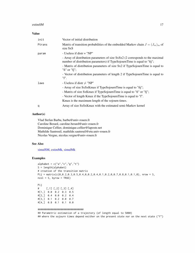
init Vector of initial distribution
Ptrans Matrix of transition probabilities of the embedded Markov chain J = (Jm)m ofsize SxS
param - Useless if distr = "NP"- Array of distribution parameters of size SxSx2 (2 corresponds to the maximalnumber of distribution parameters) if TypeSojournTime is equal to "fij";- Matrix of distribution parameters of size Sx2 if TypeSojournTime is equal to"fi" or "fj";- Vector of distribution parameters of length 2 if TypeSojournTime is equal to"f".
laws - Useless if distr 6= "NP"- Array of size SxSxKmax if TypeSojournTime is equal to "fij";- Matrix of size SxKmax if TypeSojournTime is equal to "fi" or "fj";- Vector of length Kmax if the TypeSojournTime is equal to "f".Kmax is the maximum length of the sojourn times.
q Array of size SxSxKmax with the estimated semi-Markov kernel
Author(s)
Vlad Stefan Barbu, [email protected] Berard, [email protected] Cellier, [email protected] Sautreuil, [email protected] Vergne, [email protected]
See Also
simulSM, estimMk, simulMk
Examples
alphabet = c("a","c","g","t")S = length(alphabet)# creation of the transition matrixPij = matrix(c(0,0.2,0.3,0.5,0.4,0,0.2,0.4,0.1,0.2,0,0.7,0.8,0.1,0.1,0), nrow = S,ncol = S, byrow = TRUE)
Pij# [,1] [,2] [,3] [,4]#[1,] 0.0 0.2 0.3 0.5#[2,] 0.4 0.0 0.2 0.4#[3,] 0.1 0.2 0.0 0.7#[4,] 0.8 0.1 0.1 0.0
################################## Parametric estimation of a trajectory (of length equal to 5000)## where the sojourn times depend neither on the present state nor on the next state ("f")

18 estimSM
################################## Simulation of a sequence of length 5000seq5000 = simulSM(E = alphabet, NbSeq = 1, lengthSeq = 5000, TypeSojournTime = "f",
init = c(1/4,1/4,1/4,1/4), Ptrans = Pij, distr = "pois", param = 2)
## Estimation of the simulated sequenceestSeq5000 = estimSM(seq = seq5000, E = alphabet, TypeSojournTime = "f",
distr = "pois", cens.end = 0, cens.beg = 0)
# initial distribution estimatedestSeq5000$init# [1] 0.3592058 0.1456077 0.1600481 0.3351384
# transition matrix estimatedestSeq5000$Ptrans# [,1] [,2] [,3] [,4]#[1,] 0.0000000 0.21775544 0.30150754 0.4807370#[2,] 0.4297521 0.00000000 0.18181818 0.3884298#[3,] 0.1052632 0.23308271 0.00000000 0.6616541#[4,] 0.8348294 0.08976661 0.07540395 0.0000000
# estimated parameterestSeq5000$param# [1] 2.007822 0.000000
# estimated semi-Markov kernelestSeq5000$q# , , 1# [,1] [,2] [,3] [,4]#[1,] 0.00000000 0.02924038 0.04048668 0.06455377#[2,] 0.05770747 0.00000000 0.02441470 0.05215867#[3,] 0.01413482 0.03129854 0.00000000 0.08884747#[4,] 0.11210159 0.01205393 0.01012531 0.00000000#, , 2# [,1] [,2] [,3] [,4]#[1,] 0.00000000 0.05870948 0.08129005 0.1296125#[2,] 0.11586631 0.00000000 0.04902036 0.1047253#[3,] 0.02838021 0.06284189 0.00000000 0.1783899#[4,] 0.22508003 0.02420215 0.02032981 0.0000000#, , 3# [,1] [,2] [,3] [,4]#[1,] 0.0000000 0.05893909 0.08160797 0.1301194#[2,] 0.1163195 0.00000000 0.04921208 0.1051349#[3,] 0.0284912 0.06308767 0.00000000 0.1790876#[4,] 0.2259603 0.02429681 0.02040932 0.0000000#, , 4# [,1] [,2] [,3] [,4]#[1,] 0.00000000 0.03944640 0.05461809 0.08708551#[2,] 0.07784959 0.00000000 0.03293636 0.07036405#[3,] 0.01906842 0.04222293 0.00000000 0.11985865#[4,] 0.15122935 0.01626122 0.01365943 0.00000000#, , 5
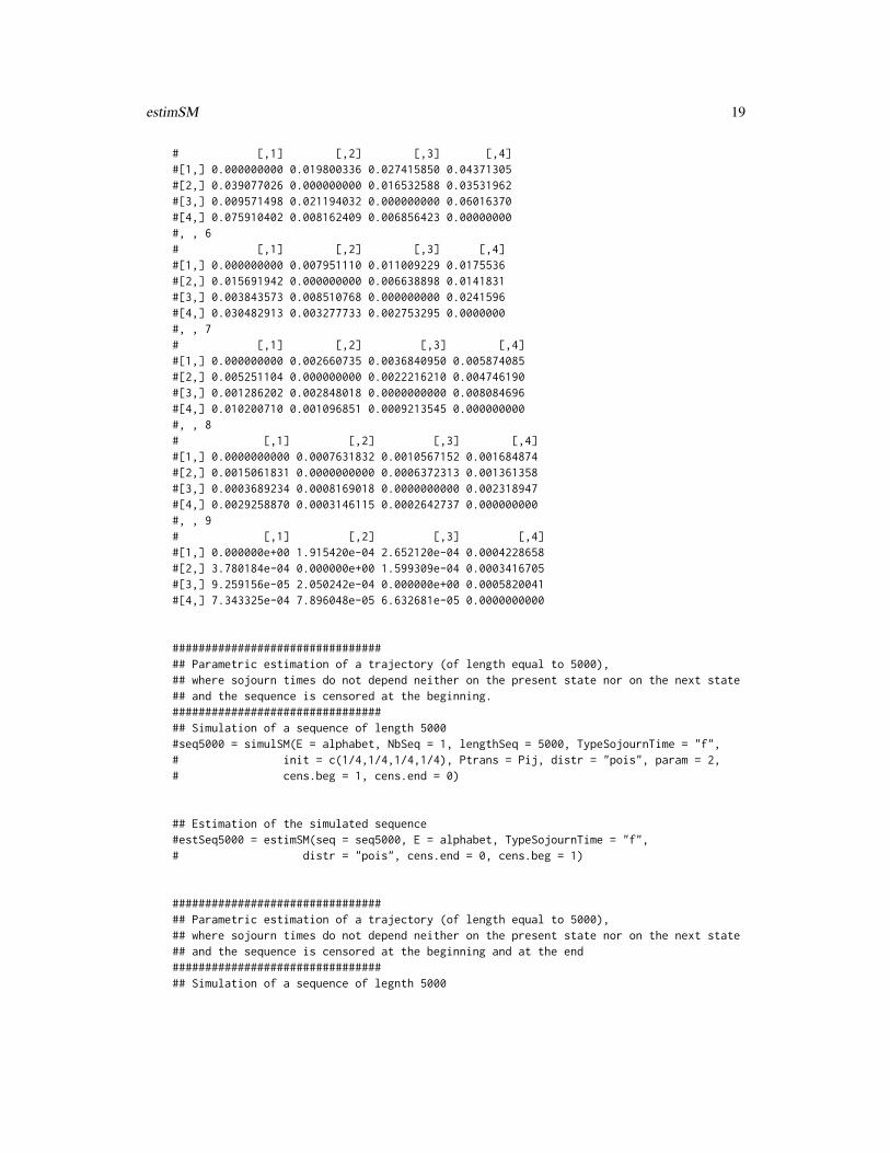
estimSM 19
# [,1] [,2] [,3] [,4]#[1,] 0.000000000 0.019800336 0.027415850 0.04371305#[2,] 0.039077026 0.000000000 0.016532588 0.03531962#[3,] 0.009571498 0.021194032 0.000000000 0.06016370#[4,] 0.075910402 0.008162409 0.006856423 0.00000000#, , 6# [,1] [,2] [,3] [,4]#[1,] 0.000000000 0.007951110 0.011009229 0.0175536#[2,] 0.015691942 0.000000000 0.006638898 0.0141831#[3,] 0.003843573 0.008510768 0.000000000 0.0241596#[4,] 0.030482913 0.003277733 0.002753295 0.0000000#, , 7# [,1] [,2] [,3] [,4]#[1,] 0.000000000 0.002660735 0.0036840950 0.005874085#[2,] 0.005251104 0.000000000 0.0022216210 0.004746190#[3,] 0.001286202 0.002848018 0.0000000000 0.008084696#[4,] 0.010200710 0.001096851 0.0009213545 0.000000000#, , 8# [,1] [,2] [,3] [,4]#[1,] 0.0000000000 0.0007631832 0.0010567152 0.001684874#[2,] 0.0015061831 0.0000000000 0.0006372313 0.001361358#[3,] 0.0003689234 0.0008169018 0.0000000000 0.002318947#[4,] 0.0029258870 0.0003146115 0.0002642737 0.000000000#, , 9# [,1] [,2] [,3] [,4]#[1,] 0.000000e+00 1.915420e-04 2.652120e-04 0.0004228658#[2,] 3.780184e-04 0.000000e+00 1.599309e-04 0.0003416705#[3,] 9.259156e-05 2.050242e-04 0.000000e+00 0.0005820041#[4,] 7.343325e-04 7.896048e-05 6.632681e-05 0.0000000000
################################## Parametric estimation of a trajectory (of length equal to 5000),## where sojourn times do not depend neither on the present state nor on the next state## and the sequence is censored at the beginning.################################## Simulation of a sequence of length 5000#seq5000 = simulSM(E = alphabet, NbSeq = 1, lengthSeq = 5000, TypeSojournTime = "f",# init = c(1/4,1/4,1/4,1/4), Ptrans = Pij, distr = "pois", param = 2,# cens.beg = 1, cens.end = 0)
## Estimation of the simulated sequence#estSeq5000 = estimSM(seq = seq5000, E = alphabet, TypeSojournTime = "f",# distr = "pois", cens.end = 0, cens.beg = 1)
################################## Parametric estimation of a trajectory (of length equal to 5000),## where sojourn times do not depend neither on the present state nor on the next state## and the sequence is censored at the beginning and at the end################################## Simulation of a sequence of legnth 5000

20 estimSM
#seq5000 = simulSM(E = alphabet, NbSeq = 1, lengthSeq = 5000, TypeSojournTime = "f",# init = c(1/4,1/4,1/4,1/4), Ptrans = Pij, distr = "pois", param = 2,# cens.beg = 1, cens.end = 1)
## Estimation of the simulated sequence#estSeq5000 = estimSM(seq = seq5000, E = alphabet, TypeSojournTime = "f",# distr = "pois", cens.end = 1, cens.beg = 1)
################################## Parametric simulation of several trajectories (3 trajectories of length 1000, 10 000## and 2000 respectively),## where the sojourn times depend on the present state and on the next state## and the sojourn time distributions are modeled by different distributions.################################lengthSeq3 = c(1000, 10000, 2000)## creation of the initial distributionvect.init = c(1/4,1/4,1/4,1/4)## creation of the distribution matrixdistr.matrix = matrix(c("dweibull", "pois", "geom", "nbinom", "geom", "nbinom","pois", "dweibull", "pois", "pois", "dweibull", "geom", "pois","geom", "geom","nbinom"), nrow = S, ncol = S, byrow = TRUE)## creation of an array containing the parametersparam1.matrix = matrix(c(0.6,2,0.4,4,0.7,2,5,0.6,2,3,0.6,0.6,4,0.3,0.4,4), nrow = S,ncol = S, byrow = TRUE)param2.matrix = matrix(c(0.8,0,0,2,0,5,0,0.8,0,0,0.8,0,4,0,0,4), nrow = S, ncol = S,byrow = TRUE)param.array = array(c(param1.matrix, param2.matrix), c(S,S,2))### Simulation of 3 sequencesseq3 = simulSM(E = alphabet, NbSeq = 3, lengthSeq = lengthSeq3, TypeSojournTime = "fij",init = vect.init, Ptrans = Pij, distr = distr.matrix, param = param.array, File.out = NULL)
## Estimation of the simulated sequenceestSeq3 = estimSM(seq = seq3, E = alphabet, TypeSojournTime = "fij",
distr = distr.matrix, cens.end = 0, cens.beg = 0)
################################## Non-Parametric simulation of several trajectories (3 trajectories of length 1000, 10 000## and 2000 respectively),## where the sojourn times depend on the present state and on the next state################################lengthSeq3 = c(1000, 10000, 2000)## creation of the initial distributionvect.init = c(1/4,1/4,1/4,1/4)## creation of an array containing the conditional distributionsKmax = 4mat1 = matrix(c(0,0.5,0.4,0.6,0.3,0,0.5,0.4,0.7,0.2,0,0.3,0.4,0.6,0.2,0), nrow = S,ncol = S, byrow = TRUE)mat2 = matrix(c(0,0.2,0.3,0.1,0.2,0,0.2,0.3,0.1,0.4,0,0.3,0.2,0.1,0.3,0), nrow = S,ncol = S, byrow = TRUE)mat3 = matrix(c(0,0.1,0.3,0.1,0.3,0,0.1,0.2,0.1,0.2,0,0.3,0.3,0.3,0.4,0), nrow = S,ncol = S, byrow = TRUE)mat4 = matrix(c(0,0.2,0,0.2,0.2,0,0.2,0.1,0.1,0.2,0,0.1,0.1,0,0.1,0), nrow = S,

estimSM 21
ncol = S, byrow = TRUE)f <- array(c(mat1,mat2,mat3,mat4), c(S,S,Kmax))### Simulation of 3 sequencesseq3.NP = simulSM(E = alphabet, NbSeq = 3, lengthSeq = lengthSeq3,TypeSojournTime = "fij", init = vect.init, Ptrans = Pij, distr = "NP", laws = f,File.out = NULL)
## Estimation of the simulated sequenceestSeq3.NP = estimSM(seq = seq3.NP, E = alphabet, TypeSojournTime = "fij",
distr = "NP", cens.end = 0, cens.beg = 0)
# initial distribution estimatedestSeq3.NP$init# [1] 0.1856190 0.2409524 0.2975714 0.2758571
# transition matrix estimatedestSeq3.NP$Ptrans# [,1] [,2] [,3] [,4]# [1,] 0.00000000 0.20560325 0.29191143 0.5024853# [2,] 0.40614334 0.00000000 0.19795222 0.3959044# [3,] 0.08932039 0.21941748 0.00000000 0.6912621# [4,] 0.81206817 0.09120221 0.09672962 0.0000000
# parameter estimatedestSeq3.NP$laws#, , 1# [,1] [,2] [,3] [,4]# [1,] 0.0000000 0.4769231 0.4009288 0.6016187# [2,] 0.3053221 0.0000000 0.4540230 0.3764368# [3,] 0.7717391 0.2389381 0.0000000 0.2794944# [4,] 0.4140669 0.5959596 0.2000000 0.0000000# , , 2# [,1] [,2] [,3] [,4]# [1,] 0.00000000 0.2175824 0.2801858 0.1052158# [2,] 0.16526611 0.0000000 0.2356322 0.2959770# [3,] 0.07608696 0.3716814 0.0000000 0.3089888# [4,] 0.18774816 0.1161616 0.3142857 0.0000000# , , 3# [,1] [,2] [,3] [,4]# [1,] 0.00000000 0.09450549 0.3188854 0.08363309# [2,] 0.31092437 0.00000000 0.1034483 0.19540230# [3,] 0.06521739 0.20353982 0.0000000 0.32022472# [4,] 0.29892229 0.28787879 0.3666667 0.00000000#, , 4# [,1] [,2] [,3] [,4]# [1,] 0.00000000 0.2109890 0.0000000 0.20953237# [2,] 0.21848739 0.0000000 0.2068966 0.13218391# [3,] 0.08695652 0.1858407 0.0000000 0.09129213# [4,] 0.09926262 0.0000000 0.1190476 0.00000000
# semi-Markovian kernel estimatedestSeq3.NP$q

22 estimSM
# , , 1# [,1] [,2] [,3] [,4]# [1,] 0.00000000 0.09805694 0.11703570 0.3023046# [2,] 0.12400455 0.00000000 0.08987486 0.1490330# [3,] 0.06893204 0.05242718 0.00000000 0.1932039# [4,] 0.33625058 0.05435283 0.01934592 0.0000000# , , 2# [,1] [,2] [,3] [,4]# [1,] 0.000000000 0.04473565 0.08178943 0.05286941# [2,] 0.067121729 0.00000000 0.04664391 0.11717861# [3,] 0.006796117 0.08155340 0.00000000 0.21359223# [4,] 0.152464302 0.01059420 0.03040074 0.00000000#, , 3# [,1] [,2] [,3] [,4]# [1,] 0.000000000 0.01943064 0.09308631 0.04202440# [2,] 0.126279863 0.00000000 0.02047782 0.07736064# [3,] 0.005825243 0.04466019 0.00000000 0.22135922# [4,] 0.242745279 0.02625518 0.03546753 0.00000000#, , 4# [,1] [,2] [,3] [,4]# [1,] 0.00000000 0.04338003 0.00000000 0.1052869# [2,] 0.08873720 0.00000000 0.04095563 0.0523322# [3,] 0.00776699 0.04077670 0.00000000 0.0631068# [4,] 0.08060801 0.00000000 0.01151543 0.0000000
#---------------------------------------------#alphabet = c("0","1")S = length(alphabet)# creation of the transition matrixPij = matrix(c(0,1,1,0), nrow = S, ncol = S, byrow = TRUE)distr = matrix(c("nbinom", "pois", "geom", "geom"), nrow = S, ncol = S, byrow = TRUE)param = array(c(matrix(c(2,5,0.4,0.7), nrow = S, ncol = S, byrow = TRUE), matrix(c(6,0,0,0),nrow = S, ncol = S, byrow = TRUE)), c(S,S,2))
################################## Parametric estimation of a trajectory (of length equal to 5000)## where the state space is {"0","1"}################################## Simulation of a sequence of length 5000seq2 = simulSM(E = alphabet, NbSeq = 2, lengthSeq = c(5000,1000), TypeSojournTime = "fij",
init = c(1/2,1/2), Ptrans = Pij, distr = distr, param = param)
## Estimation of the simulated sequenceestSeq2 = estimSM(seq = seq2, E = alphabet, TypeSojournTime = "fij",
distr = distr, cens.end = 1, cens.beg = 1)
#---------------------------------------------#
InitialLawMk 23
InitialLawMk Estimation of the initial law (Markov model)
Description
For order 1, estimation of initial law by computing the stationary law of the Markov chain.
For order greater than 1, estimation of initial law by computing the state frequencies.
Usage
InitialLawMk(E, seq, Ptrans, k)
Arguments
E Vector of state space
seq List of sequence(s)
Ptrans Matrix of transition probabilities of size (S^(k))xS, with S = length(E)
k Order of the Markov chain
Value
init Vector of the initial law
Author(s)
Vlad Stefan Barbu, [email protected] Berard, [email protected] Cellier, [email protected] Sautreuil, [email protected] Vergne, [email protected]
See Also
InitialLawMk, estimSM, simulSM, estimMk, simulMk
Examples
seq = list(c("a","c","c","g","t","a","a","a","a","g","c","t","t","t","g"))res = estimMk(seq = seq, E = c("a","c","g","t"), k = 1)p = res$Ptrans
InitialLawMk(E = c("a","c","g","t"), seq = seq, Ptrans = p, k = 1)
24 InitialLawSM
InitialLawSM Estimation of the initial law (semi-Markov model)
Description
For one sequence, estimation of the initial law by computating the limit law of the semi-Markovianchain.
For several sequences, estimation of the initial law by computating the first state frequencies.
Usage
InitialLawSM(E, seq, q)
Arguments
E Vector of state space
seq List of sequence(s)
q Array of size SxSxKmax with the semi-Markov kernel (S = length(E))
Value
init Vector of the initial distribution
Author(s)
Vlad Stefan Barbu, [email protected] Berard, [email protected] Cellier, [email protected] Sautreuil, [email protected] Vergne, [email protected]
See Also
StationaryLaw, estimSM, simulSM, estimMk, simulMk
Examples
seq = list(c("a","c","c","g","t","a","a","a","a","g","c","t","t","t","g"))res = estimSM(seq = seq, E = c("a","c","g","t"), distr = "NP")q = res$qp = res$Ptrans
InitialLawSM(E = c("a","c","g","t"), seq = seq, q = q)

LoglikelihoodMk 25
LoglikelihoodMk Loglikelihood (Markov model)
Description
Computation of the loglikelihood starting from sequence(s), alphabet, initial distribution, transitionmatrix
Usage
LoglikelihoodMk(seq, E, mu, Ptrans, k)
Arguments
seq List of sequence(s)
E Vector of state space
mu Vector of initial distribution
Ptrans Matrix of transition probabilities
k Order of the Markov chain
Value
L Value of loglikelihood for each sequence
Author(s)
Vlad Stefan Barbu, [email protected] Berard, [email protected] Cellier, [email protected] Sautreuil, [email protected] Vergne, [email protected]
See Also
simulSM, estimMk, simulMk, estimSM, LoglikelihoodSM
Examples
alphabet = c("a","c","g","t")S = length(alphabet)# creation of the transition matrixPij = matrix(c(0,0.2,0.3,0.5,0.4,0,0.2,0.4,0.1,0.2,0,0.7,0.8,0.1,0.1,0),nrow = S, ncol = S, byrow = TRUE)
#Pij# [,1] [,2] [,3] [,4]#[1,] 0.0 0.2 0.3 0.5

26 LoglikelihoodSM
#[2,] 0.4 0.0 0.2 0.4#[3,] 0.1 0.2 0.0 0.7#[4,] 0.8 0.1 0.1 0.0
## Simulation of two sequences of length 20 and 50 respectivelyseq2 = simulMk(E = alphabet, nbSeq = 2, lengthSeq = c(20,50), Ptrans = Pij,init = rep(1/4,4), k = 1)
###################################### Computation of the loglikelihood####################################LoglikelihoodMk(seq = seq2, E = alphabet, mu = rep(1/4,4), Ptrans = Pij, k = 1)
#$L#$L[[1]]#[1] -13.90161##$L[[2]]#[1] -39.58438
LoglikelihoodSM Loglikelihood (semi-Markov model)
Description
Computation of the loglikelihood starting from sequence(s), alphabet, initial distribution, transitionmatrix and type of sojourn times
Usage
## parametric caseLoglikelihoodSM(seq, E, mu, Ptrans, distr, param, laws = NULL, TypeSojournTime)## non-parametric caseLoglikelihoodSM(seq, E, mu, Ptrans, distr, param = NULL, laws, TypeSojournTime)
Arguments
seq List of sequence(s)
E Vector of state space
mu Vector of initial distribution of length S
Ptrans Matrix of transition probabilities of the embedded Markov chain J = (Jm)m ofsize SxS
distr - "NP" for nonparametric case, laws have to be used, param is useless- Matrix of distributions of size SxS if TypeSojournTime is equal to "fij";- Vector of distributions of size S if TypeSojournTime is equal to "fi" or "fj";

LoglikelihoodSM 27
- A distribution if TypeSojournTime is equal to "f".The distributions to be used in distr must be one of "uniform", "geom", "pois","dweibull", "nbinom".
param - Useless if distr = "NP"- Array of distribution parameters of size SxSx2 (2 corresponds to the maximalnumber of distribution parameters) if TypeSojournTime is equal to "fij";- Matrix of distribution parameters of size Sx2 if TypeSojournTime is equal to"fi" or "fj";- Vector of distribution parameters of length 2 if TypeSojournTime is equal to"f".
laws - Useless if distr 6= "NP"- Array of size SxSxKmax if TypeSojournTime is equal to "fij";- Matrix of size SxKmax if TypeSojournTime is equal to "fi" or "fj";- Vector of length Kmax if the TypeSojournTime is equal to "f".Kmax is the maximum length of the sojourn times.
TypeSojournTime
Character: "fij", "fi", "fj", "f" (for more explanations, see Details)
Details
In this package we can choose differents types of sojourn time. Four options are available for thesojourn times:
• depending on the present state and on the next state ("fij");
• depending only on the present state ("fi");
• depending only on the next state ("fj");
• depending neither on the current, nor on the next state ("f").
Value
L Value of loglikelihood for each sequence
Kmax The maximal observed sojourn time
Author(s)
Vlad Stefan Barbu, [email protected] Berard, [email protected] Cellier, [email protected] Sautreuil, [email protected] Vergne, [email protected]
See Also
simulSM, estimMk, simulMk, estimSM
28 LoglikelihoodSM
Examples
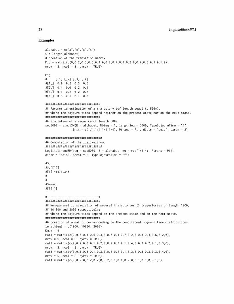
alphabet = c("a","c","g","t")S = length(alphabet)# creation of the transition matrixPij = matrix(c(0,0.2,0.3,0.5,0.4,0,0.2,0.4,0.1,0.2,0,0.7,0.8,0.1,0.1,0),nrow = S, ncol = S, byrow = TRUE)
Pij# [,1] [,2] [,3] [,4]#[1,] 0.0 0.2 0.3 0.5#[2,] 0.4 0.0 0.2 0.4#[3,] 0.1 0.2 0.0 0.7#[4,] 0.8 0.1 0.1 0.0
################################## Parametric estimation of a trajectory (of length equal to 5000),## where the sojourn times depend neither on the present state nor on the next state.################################## Simulation of a sequence of length 5000seq5000 = simulSM(E = alphabet, NbSeq = 1, lengthSeq = 5000, TypeSojournTime = "f",
init = c(1/4,1/4,1/4,1/4), Ptrans = Pij, distr = "pois", param = 2)
################################### Computation of the loglikelihood#################################LoglikelihoodSM(seq = seq5000, E = alphabet, mu = rep(1/4,4), Ptrans = Pij,distr = "pois", param = 2, TypeSojournTime = "f")
#$L#$L[[1]]#[1] -1475.348###$Kmax#[1] 10
#------------------------------################################### Non-parametric simulation of several trajectories (3 trajectories of length 1000,## 10 000 and 2000 respectively),## where the sojourn times depend on the present state and on the next state.################################## creation of a matrix corresponding to the conditional sojourn time distributionslengthSeq3 = c(1000, 10000, 2000)Kmax = 4mat1 = matrix(c(0,0.5,0.4,0.6,0.3,0,0.5,0.4,0.7,0.2,0,0.3,0.4,0.6,0.2,0),nrow = S, ncol = S, byrow = TRUE)mat2 = matrix(c(0,0.2,0.3,0.1,0.2,0,0.2,0.3,0.1,0.4,0,0.3,0.2,0.1,0.3,0),nrow = S, ncol = S, byrow = TRUE)mat3 = matrix(c(0,0.1,0.3,0.1,0.3,0,0.1,0.2,0.1,0.2,0,0.3,0.3,0.3,0.4,0),nrow = S, ncol = S, byrow = TRUE)mat4 = matrix(c(0,0.2,0,0.2,0.2,0,0.2,0.1,0.1,0.2,0,0.1,0.1,0,0.1,0),
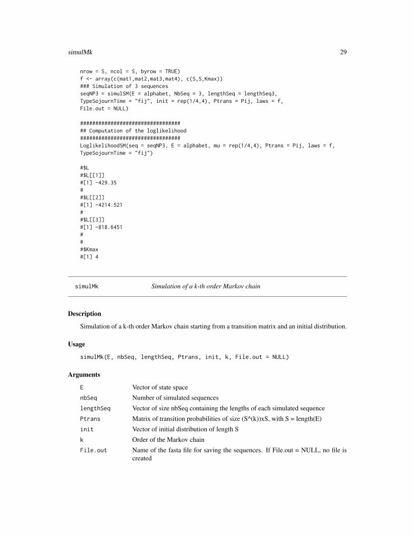
simulMk 29
nrow = S, ncol = S, byrow = TRUE)f <- array(c(mat1,mat2,mat3,mat4), c(S,S,Kmax))### Simulation of 3 sequencesseqNP3 = simulSM(E = alphabet, NbSeq = 3, lengthSeq = lengthSeq3,TypeSojournTime = "fij", init = rep(1/4,4), Ptrans = Pij, laws = f,File.out = NULL)
################################### Computation of the loglikelihood#################################LoglikelihoodSM(seq = seqNP3, E = alphabet, mu = rep(1/4,4), Ptrans = Pij, laws = f,TypeSojournTime = "fij")
#$L#$L[[1]]#[1] -429.35##$L[[2]]#[1] -4214.521##$L[[3]]#[1] -818.6451###$Kmax#[1] 4
simulMk Simulation of a k-th order Markov chain
Description
Simulation of a k-th order Markov chain starting from a transition matrix and an initial distribution.
Usage
simulMk(E, nbSeq, lengthSeq, Ptrans, init, k, File.out = NULL)
Arguments
E Vector of state space
nbSeq Number of simulated sequences
lengthSeq Vector of size nbSeq containing the lengths of each simulated sequence
Ptrans Matrix of transition probabilities of size (S^(k))xS, with S = length(E)
init Vector of initial distribution of length S
k Order of the Markov chain
File.out Name of the fasta file for saving the sequences. If File.out = NULL, no file iscreated

30 simulMk
Details
The sizes of init and Ptrans depend on S, the length of E. The rows of the transition matrix sums to1.
For k=1, the transition matrix is defined by Ptrans(i, j) = P (Xm+1 = j|Xm = i) and the initialdistribution is init = P (X1 = i). For k > 1 we have similar expressions.
The first element of lengthSeq corresponds to the length of the first sequence and so on.
Value
simulMk returns a list of sequences of size lengthSeq simulated with a k-th order Markov chain ofparameters init and Ptrans with state space E.
If the parameter File.out is not equal to NULL, a file in fasta format containing the sequence(s) willbe created.
Author(s)
Vlad Stefan Barbu, [email protected] Berard, [email protected] Cellier, [email protected] Sautreuil, [email protected] Vergne, [email protected]
See Also
estimMk, simulSM, estimSM
Examples
### Example 1 #### Second order model with state space {a,c,g,t}E <- c("a","c","g","t")S = length(E)init.distribution <- c(1/6,1/6,5/12,3/12)k<-2p <- matrix(0.25, nrow = S^k, ncol = S)
# We simulate 3 sequences of size 1000, 10000 and 2000 respectively.simulMk(E = E, nbSeq = 3, lengthSeq = c(1000, 10000, 2000), Ptrans = p,init = init.distribution, k = k)
### Example 2 #### first order model with state space {1,2,3}E <- c(1,2,3)S <- length(E)init.distr <- rep(1/S, 3)p <- matrix(c(0.3,0.2,0.5,0.1,0.6,0.3,0.2,0.4,0.4), nrow = 3, byrow = TRUE)
# We simulate one sequence of size 100simulMk(E = E, nbSeq = 1, lengthSeq = 100, Ptrans = p, init = init.distr, k = 1)
simulSM 31
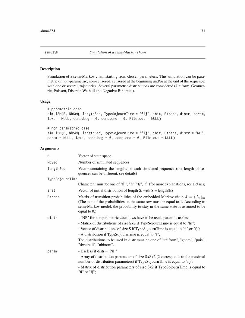
simulSM Simulation of a semi-Markov chain
Description
Simulation of a semi-Markov chain starting from chosen parameters. This simulation can be para-metric or non-parametric, non-censored, censored at the beginning and/or at the end of the sequence,with one or several trajectories. Several parametric distributions are considered (Uniform, Geomet-ric, Poisson, Discrete Weibull and Negative Binomial).
Usage
# parametric casesimulSM(E, NbSeq, lengthSeq, TypeSojournTime = "fij", init, Ptrans, distr, param,laws = NULL, cens.beg = 0, cens.end = 0, File.out = NULL)
# non-parametric casesimulSM(E, NbSeq, lengthSeq, TypeSojournTime = "fij", init, Ptrans, distr = "NP",param = NULL, laws, cens.beg = 0, cens.end = 0, File.out = NULL)
Arguments
E Vector of state space
NbSeq Number of simulated sequences
lengthSeq Vector containing the lengths of each simulated sequence (the length of se-quences can be different, see details)
TypeSojournTime
Character : must be one of "fij", "fi", "fj", "f" (for more explanations, see Details)
init Vector of initial distribution of length S, with S = length(E)
Ptrans Matrix of transition probabilities of the embedded Markov chain J = (Jm)m(The sum of the probabilities on the same row must be equal to 1. According tosemi-Markov model, the probability to stay in the same state is assumed to beequal to 0.)
distr - "NP" for nonparametric case, laws have to be used, param is useless- Matrix of distributions of size SxS if TypeSojournTime is equal to "fij";- Vector of distributions of size S if TypeSojournTime is equal to "fi" or "fj";- A distribution if TypeSojournTime is equal to "f".The distributions to be used in distr must be one of "uniform", "geom", "pois","dweibull", "nbinom".
param - Useless if distr = "NP"- Array of distribution parameters of size SxSx2 (2 corresponds to the maximalnumber of distribution parameters) if TypeSojournTime is equal to "fij";- Matrix of distribution parameters of size Sx2 if TypeSojournTime is equal to"fi" or "fj";

32 simulSM
- Vector of distribution parameters of length 2 if TypeSojournTime is equal to"f".
laws - Useless if distr 6= "NP"- Array of size SxSxKmax if TypeSojournTime is equal to "fij";- Matrix of size SxKmax if TypeSojournTime is equal to "fi" or "fj";- Vector of length Kmax if the TypeSojournTime is equal to "f".Kmax is the maximum length of the sojourn times.
cens.beg Type of censoring at the beginning of sample paths; 1 (if the first sojourn timeis censored) or 0 (if not). All the sequences must be censored in the same way.
cens.end Type of censoring at the end of sample paths; 1 (if the last sojourn time is cen-sored) or 0 (if not). All the sequences must be censored in the same way.
File.out Name of fasta file to save the sequences; if File.out = NULL, no file is created.
Details
This function simulates a semi-Markov model in the parametric and non-parametric case, takinginto account the type of sojourn time and the censoring described in references.
The non-parametric simulation concerns sojourn time distributions defined by the user. For theparametric simulation, several discrete distributions are considered (see below).
The difference between the Markov model and the semi-Markov model concerns the modelling ofthe sojourn time. With a Markov chain, the sojourn time distribution is modeled by a Geometricdistribution. With a semi-Markov chain, the sojourn time can be arbitrarily distributed. In thispackage, the available distribution for a semi-Markov model are:
• Uniform: f(x) = 1/n for a ≤ x ≤ b, with n = b− a+ 1
• Geometric: f(x) = θ(1 − θ)x for x = 0, 1, 2, . . . , n, 0 < θ ≤ 1, with n > 0 and θ is theprobability of success
• Poisson: f(x) = (λxexp(−λ))/x! for x = 0, 1, 2, . . . , n, with n > 0 and λ > 0
• Discrete Weibull of type 1: f(x) = q(x−1)β − qxβ
, x = 1, 2, 3, . . . , n, with n > 0, q is thefirst parameter and β is the second parameter
• Negative Binomial: f(x) = Γ(x+α)/(Γ(α)x!)(α/(α+µ))α(µ/(α+µ))x, for x = 0, 1, 2, . . . , n,n > 0, Γ is the gamma function, α is the parameter of overdispersion and µ is the mean
• Non-parametric
We define :
• the semi-Markov kernel qij(k) = P (Jm+1 = j, Tm+1 − Tm = k|Jm = i);
• the transition matrix (Ptrans(i, j))i,j ∈ E of the embedded Markov chain J = (Jm)m,Ptrans(i, j) = P (Jm+1 = j|Jm = i);
• the initial distribution, init = P (J1 = i) = P (Y1 = i);
• the conditional sojourn time distributions (fij(k))i,j ∈ E, k ∈ N, fij(k) = P (Tm+1−Tm =k|Jm = i, Jm+1 = j), f is specified by the argument "param" in the parametric case and by"laws" in the non-parametric case.
In this package we can choose differents types of sojourn times. Four options are available for thesojourn times
simulSM 33
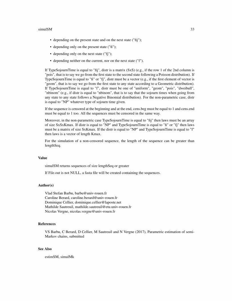
• depending on the present state and on the next state ("fij");
• depending only on the present state ("fi");
• depending only on the next state ("fj");
• depending neither on the current, nor on the next state ("f").
If TypeSojournTime is equal to "fij", distr is a matrix (SxS) (e.g., if the row 1 of the 2nd column is"pois", that is to say we go from the first state to the second state following a Poisson distribution). IfTypeSojournTime is equal to "fi" or "fj", distr must be a vector (e.g., if the first element of vector is"geom", that is to say we go from the first state to any state according to a Geometric distribution).If TypeSojournTime is equal to "f", distr must be one of "uniform", "geom", "pois", "dweibull","nbinom" (e.g., if distr is equal to "nbinom", that is to say that the sojourn times when going fromany state to any state follows a Negative Binomial distribution). For the non-parametric case, distris equal to "NP" whatever type of sojourn time given.
If the sequence is censored at the beginning and at the end, cens.beg must be equal to 1 and cens.endmust be equal to 1 too. All the sequences must be censored in the same way.
Moreover, in the non-parametric case TypeSojournTime is equal to "fij" then laws must be an arrayof size SxSxKmax. If distr is equal to "NP" and TypeSojournTime is equal to "fi" or "fj" then lawsmust be a matrix of size SxKmax. If the distr is equal to "NP" and TypeSojournTime is equal to "f"then laws is a vector of length Kmax.
For the simulation of a non-censored sequence, the length of the sequence can be greater thanlengthSeq.
Value
simulSM returns sequences of size lengthSeq or greater
If File.out is not NULL, a fasta file will be created containing the sequences.
Author(s)
Vlad Stefan Barbu, [email protected] Berard, [email protected] Cellier, [email protected] Sautreuil, [email protected] Vergne, [email protected]
References
VS Barbu, C Berard, D Cellier, M Sautreuil and N Vergne (2017), Parametric estimation of semi-Markov chains, submitted
See Also
estimSM, simulMk
34 simulSM
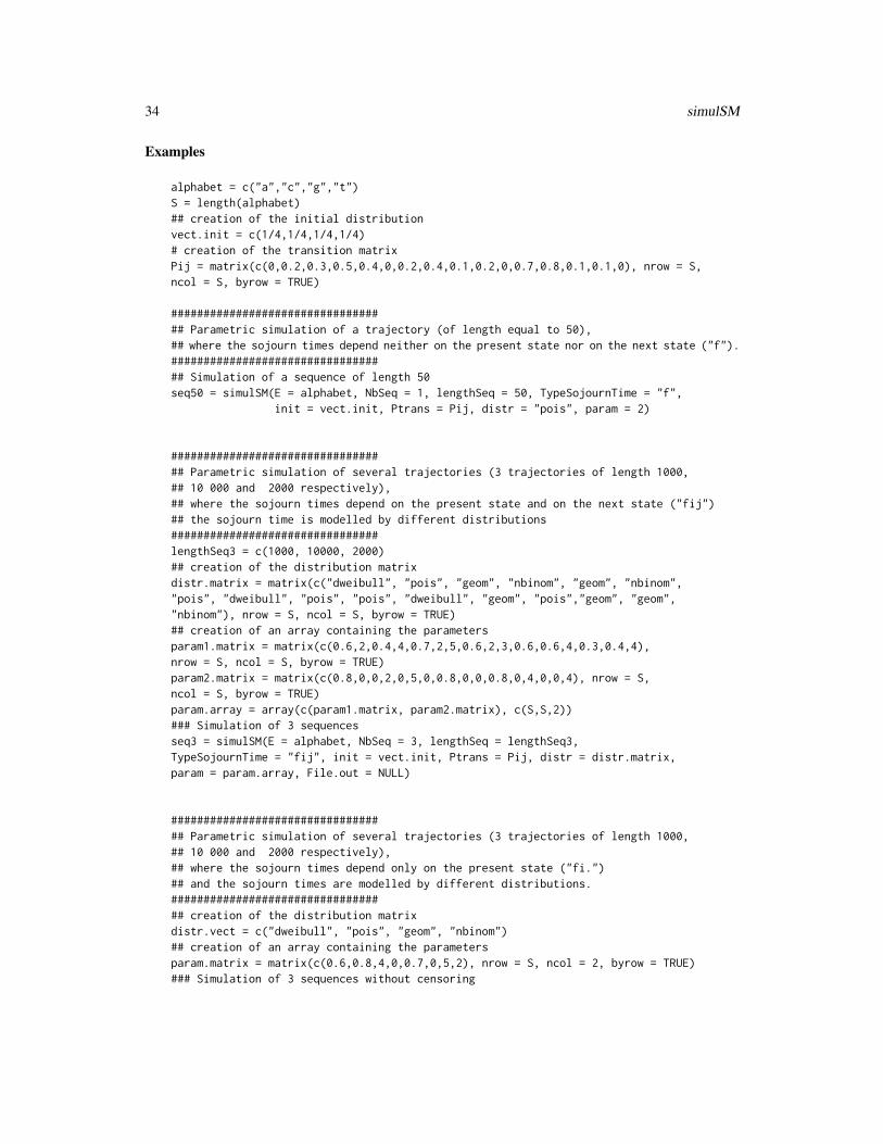
Examples
alphabet = c("a","c","g","t")S = length(alphabet)## creation of the initial distributionvect.init = c(1/4,1/4,1/4,1/4)# creation of the transition matrixPij = matrix(c(0,0.2,0.3,0.5,0.4,0,0.2,0.4,0.1,0.2,0,0.7,0.8,0.1,0.1,0), nrow = S,ncol = S, byrow = TRUE)
################################## Parametric simulation of a trajectory (of length equal to 50),## where the sojourn times depend neither on the present state nor on the next state ("f").################################## Simulation of a sequence of length 50seq50 = simulSM(E = alphabet, NbSeq = 1, lengthSeq = 50, TypeSojournTime = "f",
init = vect.init, Ptrans = Pij, distr = "pois", param = 2)
################################## Parametric simulation of several trajectories (3 trajectories of length 1000,## 10 000 and 2000 respectively),## where the sojourn times depend on the present state and on the next state ("fij")## the sojourn time is modelled by different distributions################################lengthSeq3 = c(1000, 10000, 2000)## creation of the distribution matrixdistr.matrix = matrix(c("dweibull", "pois", "geom", "nbinom", "geom", "nbinom","pois", "dweibull", "pois", "pois", "dweibull", "geom", "pois","geom", "geom","nbinom"), nrow = S, ncol = S, byrow = TRUE)## creation of an array containing the parametersparam1.matrix = matrix(c(0.6,2,0.4,4,0.7,2,5,0.6,2,3,0.6,0.6,4,0.3,0.4,4),nrow = S, ncol = S, byrow = TRUE)param2.matrix = matrix(c(0.8,0,0,2,0,5,0,0.8,0,0,0.8,0,4,0,0,4), nrow = S,ncol = S, byrow = TRUE)param.array = array(c(param1.matrix, param2.matrix), c(S,S,2))### Simulation of 3 sequencesseq3 = simulSM(E = alphabet, NbSeq = 3, lengthSeq = lengthSeq3,TypeSojournTime = "fij", init = vect.init, Ptrans = Pij, distr = distr.matrix,param = param.array, File.out = NULL)
################################## Parametric simulation of several trajectories (3 trajectories of length 1000,## 10 000 and 2000 respectively),## where the sojourn times depend only on the present state ("fi.")## and the sojourn times are modelled by different distributions.################################## creation of the distribution matrixdistr.vect = c("dweibull", "pois", "geom", "nbinom")## creation of an array containing the parametersparam.matrix = matrix(c(0.6,0.8,4,0,0.7,0,5,2), nrow = S, ncol = 2, byrow = TRUE)### Simulation of 3 sequences without censoring
simulSM 35
#seqFi3 = simulSM(E = alphabet, NbSeq = 3, lengthSeq = lengthSeq3, TypeSojournTime = "fi",# init = vect.init, Ptrans = Pij, distr = distr.vect, param = param.matrix,# File.out = NULL)### Simulation of 3 sequences with censoring at the beginning#seqFi3 = simulSM(E = alphabet, NbSeq = 3, lengthSeq = lengthSeq3, TypeSojournTime = "fi",# init = vect.init, Ptrans = Pij, distr = distr.vect, param = param.matrix,# File.out = NULL, cens.beg = 1, cens.end = 0)### Simulation of 3 sequences with censoring at the end#seqFi3 = simulSM(E = alphabet, NbSeq = 3, lengthSeq = lengthSeq3, TypeSojournTime = "fi",# init = vect.init, Ptrans = Pij, distr = distr.vect, param = param.matrix,# File.out = NULL, cens.beg = 0, cens.end = 1)### Simulation of 3 sequences with censoring at the beginning and at the end#seqFi3 = simulSM(E = alphabet, NbSeq = 3, lengthSeq = lengthSeq3, TypeSojournTime = "fi",# init = vect.init, Ptrans = Pij, distr = distr.vect, param = param.matrix,# File.out = NULL, cens.beg = 1, cens.end = 1)
################################## Non-parametric simulation of several trajectories (3 trajectories of length 1000,## 10 000 and 2000 respectively),## where the sojourn times depend on the present state and on the next state ("fij")################################## creation of a matrix corresponding to the conditionnal sojourn time distributionKmax = 4mat1 = matrix(c(0,0.5,0.4,0.6,0.3,0,0.5,0.4,0.7,0.2,0,0.3,0.4,0.6,0.2,0), nrow = S,ncol = S, byrow = TRUE)mat2 = matrix(c(0,0.2,0.3,0.1,0.2,0,0.2,0.3,0.1,0.4,0,0.3,0.2,0.1,0.3,0), nrow = S,ncol = S, byrow = TRUE)mat3 = matrix(c(0,0.1,0.3,0.1,0.3,0,0.1,0.2,0.1,0.2,0,0.3,0.3,0.3,0.4,0), nrow = S,ncol = S, byrow = TRUE)mat4 = matrix(c(0,0.2,0,0.2,0.2,0,0.2,0.1,0.1,0.2,0,0.1,0.1,0,0.1,0), nrow = S,ncol = S, byrow = TRUE)f <- array(c(mat1,mat2,mat3,mat4), c(S,S,Kmax))### Simulation of 3 sequencesseqNP3 = simulSM(E = alphabet, NbSeq = 3, lengthSeq = lengthSeq3, TypeSojournTime = "fij",
init = vect.init, Ptrans = Pij, laws = f, File.out = NULL)
################################## Non-parametric simulation of several trajectories (3 trajectories of length 1000,## 10 000 and 2000 respectively),## where the sojourn times depend only on he next state ("fj")################################## creation of a matrix corresponding to the conditional sojourn time distributionsKmax = 6nparam.matrix = matrix(c(0.2,0.1,0.3,0.2,0.2,0,0.4,0.2,0.1,0,0.2,0.1,0.5,0.3,0.15,0.05,0,0,0.3,0.2,0.1,0.2,0.2,0),
nrow = S, ncol = Kmax, byrow = TRUE)### Simulation of 3 sequences without censoring#seqNP3 = simulSM(E = alphabet, NbSeq = 3, lengthSeq = lengthSeq3, TypeSojournTime = "fj",# init = vect.init, Ptrans = Pij, laws = nparam.matrix, File.out = NULL)### Simulation of 3 sequences with censoring at the beginnig#seqNP3 = simulSM(E = alphabet, NbSeq = 3, lengthSeq = lengthSeq3, TypeSojournTime = "fj",# init = vect.init, Ptrans = Pij, laws = nparam.matrix, File.out = NULL,

36 simulSM
# cens.beg = 1, cens.end = 0)### Simulation of 3 sequences with censoring at the end#seqNP3 = simulSM(E = alphabet, NbSeq = 3, lengthSeq = lengthSeq3, TypeSojournTime = "fj",# init = vect.init, Ptrans = Pij, laws = nparam.matrix, File.out = NULL,# cens.beg = 0, cens.end = 1)### Simulation of 3 sequences with censoring at the beginning and at the end#seqNP3 = simulSM(E = alphabet, NbSeq = 3, lengthSeq = lengthSeq3, TypeSojournTime = "fj",# init = vect.init, Ptrans = Pij, laws = nparam.matrix, File.out = NULL,# cens.beg = 1, cens.end = 1)

Index
∗Topic AICAIC_Mk, 4AIC_SM, 6
∗Topic BICBIC_Mk, 8BIC_SM, 10
∗Topic Censored dataSMM-package, 2
∗Topic EstimationestimMk, 12estimSM, 14SMM-package, 2
∗Topic LoglikelihoodLoglikelihoodMk, 25LoglikelihoodSM, 26
∗Topic Markov modelsAIC_Mk, 4BIC_Mk, 8estimMk, 12InitialLawMk, 23LoglikelihoodMk, 25simulMk, 29SMM-package, 2
∗Topic Semi-Markov modelsAIC_SM, 6BIC_SM, 10estimSM, 14InitialLawSM, 24LoglikelihoodSM, 26simulSM, 31SMM-package, 2
∗Topic SimulationsimulMk, 29simulSM, 31SMM-package, 2
AIC_Mk, 4, 7, 9AIC_SM, 6, 11
BIC_Mk, 8, 11
BIC_SM, 10
estimMk, 2, 5, 7, 9, 11, 12, 17, 25, 27estimSM, 2, 5, 7, 9, 11, 14, 25, 27
InitialLawMk, 23InitialLawSM, 24
LoglikelihoodMk, 5, 7, 9, 11, 25LoglikelihoodSM, 5, 7, 9, 11, 25, 26
simulMk, 2, 5, 7, 9, 11, 17, 25, 27, 29simulSM, 2, 5, 7, 9, 11, 17, 25, 27, 31SMM (SMM-package), 2SMM-package, 2
37