The matching method for treatment evaluation with selective participation

and ineligibles

Monica Costa Dias Hidehiko Ichimura

Gerard J. van den Berg

WORKING PAPER 2008:6

The Institute for Labour Market Policy Evaluation (IFAU) is a research institute under the Swedish Ministry of Employment, situated in Uppsala. IFAU’s objective is to promote, support and carry out scientific evaluations. The assignment includes: the effects of labour market policies, studies of the functioning of the labour market, the labour market effects of educational policies and the labour market effects of social insurance policies. IFAU shall also disseminate its results so that they become acces­sible to different interested parties in Sweden and abroad.

IFAU also provides funding for research projects within its areas of interest. The deadline for applications is October 1 each year. Since the researchers at IFAU are mainly economists, researchers from other disciplines are encouraged to apply for funding.

IFAU is run by a Director-General. The institute has a scientific council, consisting of a chairman, the Director-General and five other members. Among other things, the scientific council proposes a decision for the allocation of research grants. A reference group including representatives for employer organizations and trade unions, as well as the ministries and authorities concerned is also connected to the institute.

Postal address: P O Box 513, 751 20 Uppsala Visiting address: Kyrkogårdsgatan 6, Uppsala Phone: +46 18 471 70 70 Fax: +46 18 471 70 71 ifau@ifau.uu.se www.ifau.se

Papers published in the Working Paper Series should, according to the IFAU policy, have been discussed at seminars held at IFAU and at least one other academic forum, and have been read by one external and one internal referee. They need not, however, have undergone the standard scrutiny for publication in a scientific journal. The purpose of the Working Paper Series is to provide a factual basis for public policy and the public policy discussion.

ISSN 1651-1166

The matching method for treatment evaluation with selective participation

and ineligibles

Monica Costa Dias∗

Hidehiko Ichimura†

Gerard J. van den Berg‡

April 21, 2008

Abstract

The matching method for treatment evaluation does not balance selec­tive unobserved differences between treated and non-treated. We derive a simple correction term if there is an instrument that shifts the treatment probability to zero in specific cases. Policies with eligibility restrictions, where treatment is impossible if some variable exceeds a certain value, pro­vide a natural application. In an empirical analysis, we first examine the performance of matching versus regression-discontinuity estimation in the sharp age-discontinuity design of the NDYP job search assistance program for young unemployed in the UK. Next, we exploit the age eligibility re­striction in the Swedish Youth Practice subsidized work program for young unemployed, where compliance is imperfect among the young. Adjusting the matching estimator for selectivity changes the results towards ineffec­tiveness of subsidized work in moving individuals into employment.

∗IFS, Cemmap and UCL †University of Tokyo. ‡VU University Amsterdam, IFAU-Uppsala, Netspar, CEPR, IZA, and IFS. Address: De­

partment of Economics, VU University Amsterdam, De Boelelaan 1105, 1081 HV Amsterdam, The Netherlands.

Keywords: propensity score, policy evaluation, treatment effect, regression discontinuity, selection, job search assistance, subsidized work, youth unemployment. JEL codes: J64, C14, C25. Acknowledgements: We thank Richard Blundell, Xavier de Luna, Paul Gregg, Barbara Sianesi, and Petra Todd, for useful comments. We also thank Louise Kennerberg and Barbara Sianesi for help with the Swedish data. We gratefully acknowledge financial support from the ESRC and from IFAU-Uppsala.

1 Introduction

The matching method for treatment evaluation compares outcomes of treated and non-treated subjects, conditioning on observed characteristics of the subjects and their environment. Basically, the average treatment effect on the treated (ATT) is estimated by averaging observed outcome differences over the treated. The main assumption is that the conditioning ensures that the assigned treatment status is conditionally mean independent from the potential outcomes (this is usually known as “the Conditional Independence Assumption” or, in short, CIA although in fact it respects to the mean; we follow the common practice and call it CIA).1

The method is intuitive, as it mimics randomized experiments: the distribu­

tions of behavioral determinants and indicators are balanced as closely as possible over treated and non-treated, using observational data. The use of the method has improved the policy evaluation practice by clarifying the importance of com­

mon support restrictions for the distribution of conditioning variables. By now, it is a common tool for the analysis of active labor market policies (ALMP) and programs (see e.g. the survey in Kluve, 2006).

A well-recognized limitation of matching is that it does not ensure the bal­

ancing of the distributions of unobserved determinants of treatment assignment among treated and non-treated. If the assigned treatment as well as the poten­

tial outcomes are affected by unobserved characteristics, and if these are not fully explained by the set of conditioning variables, the matching may give biased re­sults. This is a potentially serious concern in the case of the evaluation of ALMP for unemployed workers. Observed individual characteristics and past individual labor market outcomes may not fully capture individual’s motivation and social skills, and the latter may affect both the case workers’ treatment assignment and the unemployed individuals’ job prospects.2

The first contribution of this paper is to derive a simple adjustment or correc­

tion term for the matching estimator for the case where treated and non-treated are systematically different in unobserved characteristics affecting the potential outcomes. Key to this is the existence of an instrumental variable that affects

1See e.g. Cochrane and Rubin (1973), Rosenbaum and Rubin (1983), and Heckman, Ichimura, and Todd (1998).

2For example, Card and Sullivan (1988), Gritz (1993), Bonnal, Fougere and Serandon (1997) and Richardson and Van den Berg (2001) argue that this can be expected to play a major role in the empirical evaluation of ALMP, and their estimation results confirm this. Van den Berg, Van der Klaauw and Van Ours (2004) contain similar findings for the effect of punitive sanctions for welfare recipients.

2

the treatment decision but not outcome. In particular, the variable is required to shift the treatment probability to zero for a specific (limiting) value of the variable. This allows for estimation of the mean outcome among controls that is free from any selection problem, which in turn allows for estimation of the counterfactual mean outcome without treatment among those who are actually treated. The correction term for selectivity is zero in case of conditional mean independence, and this applies if the value of the instrument is observed not to covary with the outcome among non-treated individuals.3 With the instrument, we can thus test whether the matching method is appropriate (i.e., whether the CIA is satisfied).

The method is particularly useful if the policy design contains an eligibility boundary restriction in the sense that treatment is impossible if some observed variable or characteristic exceeds a certain threshold value, while individuals are eligible for the treatment on the other side of the threshold value but they are sometimes not treated. In other words, individuals whose characteristic exceeds a certain threshold value are not eligible, and this is strictly enforced, while individuals whose characteristic is below the threshold are eligible, but their compliance is imperfect. Here, the word “compliance” is used in a statistical sense, meaning that individuals who according to the policy design are eligible for treatment end up in the non-treated subpopulation.

This is a relevant setting. It is a common feature of ALMP to restrict eligibility to individuals aged above or below a certain age, and/or to individuals with a certain minimum or maximum amount of education, and/or to individuals with a certain minimum amount of labor market experience (see e.g. Kluve, 2006).4 If imperfect compliance among the eligible individuals is selective then the matching approach cannot be used. Our approach overcomes this limitation, by exploiting the eligibility boundary restriction within the matching framework.

Our work is in the spirit of Battistin and Rettore (2007), who study the per­

formance of matching within a special discontinuity design where non-compliance

3Alternative approaches in order to correct matching estimators for selection problems typ­ically assume that the relevant unobserved variables have additive effects on the potential outcomes (see Heckman and Robb, 1985, and Andrews and Schafgans, 1998). The popular conditional difference-in-differences estimator (Heckman, Ichimura, Smith, and Todd, 1998) is also based on this. By contrast, our approach does not require additivity.

4Sometimes the boundary restrictions are based on a variable or set of variables that can be used as instruments only locally. This is the case, for example, of employment programs establishing eligibility on the basis of unemployment duration. In such cases, a regression discontinuity approach may be more adequate if the restriction introduces a discontinuity in the participation rate.

3

affects decisions only on one side of the discontinuity (see also Angrist and Im-

bens, 1991, and Van der Klaauw, 2008, for inference using regression discontinuity with imperfect compliance). However, by exploiting the existence of an instru­

ment we are able to depart from the discontinuity case and focus on global rather than local parameters. We also develop a (global) test of the matching CIA assumption.

We empirically assess our approach by evaluating two major ALMP aimed at helping unemployed individuals aged below 25 to find work.5 First of all, we estimate the average effect of participation in the New Deal for Young People (NDYP) program for young unemployed in the UK on the individual probabil­

ity of finding work. Participants enter the program upon reaching 6 months of unemployment. From that moment until 4 months later, they receive intensive job search assistance. The program provides a sharp age-discontinuity design in that participation is compulsory for, and restricted to, those aged below 25 upon reaching 6 months of unemployment. As such, the inference method that we develop in this paper cannot be applied here. Nevertheless, we feel that the NDYP analysis is relevant because it allows us to assess the performance of matching in a setting where it should correctly estimate the ATT (for an ap­

propriate subpopulation). For the usefulness of our method, it seems reasonable to demand that matching performs well in a sharp discontinuity design if the instrument is the variable underlying the eligibility. This evaluation can be seen as a non-experimental counterpart of LaLonde (1986)’ s validation study with experimental data. When we use matching then we obviously do not include age in the set of explanatory variables in the NDYP propensity score. As such, we examine whether matching is able to capture the NDYP assignment process that in reality is only driven by age at 6 months of unemployment.

We should emphasize that, in general, if the CIA is valid, matching estimators and regression-discontinuity estimators do not necessarily estimate the same av­

erage effect. Specifically, the latter estimates a local effect for the subpopulation of individuals close to the eligibility threshold, whereas the former may estimate a global ATT effect for a wider group of treated. To prevent a misalignment of subpopulations, we restrict attention in all analyses to individuals close to the eligibility threshold. In order to detect secular effects of age, we repeat the anal­

yses at integer age changes within the set of eligible individuals. A differential

5There is an increasing awareness that youth unemployment may be a serious problem for society despite the fact that youth unemployment durations are relatively short. This is because of the prevalence of psychological and labor-market scarring effects which may have long-run implications for the productivity of those affected (see e.g. Burgess et al., 2003).

4

effect for e.g. those aged 23.99 and those aged 24.01 should be taken into account when exploiting the eligibility threshold at age 25.

Next, in our second empirical evaluation, we estimate the average employ­

ment effect of participation in the Swedish Youth Practice (YP) subsidized work program for young unemployed. This program is designed for short-term unem­

ployed individuals aged below 25. The program is not compulsory, being one among a number of alternative treatments. This means that compliance is im­

perfect on the lower side of the age-eligibility threshold. We may therefore apply our selectivity-adjusted matching estimator. The subpopulation of non-treated includes those below 25 who do not participate as well as those above 25. In fact, participation is not sharply discontinuous at age 25 but declines shortly before age 25. This is not a problem for our method but would complicate the use of regression-discontinuity methods.

Both the British NDYP and the Swedish YP have been evaluated before, in a range of studies (see e.g. Blundell et al., 2004, De Giorgi, 2005, Larsson, 2003, and Forslund and Nordstrom Skans, 2006, for results and overviews of results).6

It is of particular interest that the YP evaluations are based on the matching approach and that we find that adjusting the matching estimator for selectivity changes the results towards ineffectiveness of YP.

In Section 2 we develop a formal framework for the analysis. We define the objects of interest and we derive the selectivity-adjusted matching estimator. In Sections 3 and 4 we evaluate the British NDYP program and the Swedish YP program, respectively. Section 5 discusses our results within the existing literature. Section 6 concludes.

2 Inference

We adopt standard counterfactual notation where Y0 and Y1 are individual coun­

terfactual outcomes associated with being assigned to non-treatment and treat­

ment, respectively. The binary indicator D denotes the actual treatment status. The vector X contains conditioning variables.

Suppose there exists an instrumental variable Z satisfying the following con­

ditions,

1. Y0 ⊥ Z | X;

6See White and Knight (2002), for an explicit descriptive comparison of the NDYP and YP programs.

5

2. There exists a set of points {z ∗ , z ∗∗} in the domain of Z where P [D = 0 | X, Z = z ∗] = 1 and 0 < P [D = 0 | X, Z = z ∗∗] < 1.

In this case,

E [Y0 | X] = E [Y0 | X, Z]

= E [Y0 | X, Z, D = 0] P [D = 0 | X, Z] +

E [Y0 | X, Z, D = 1] P [D = 1 | X, Z] .

Since this relationship holds for all possible values of Z, and in particular for Z = z ∗, it yields

E [Y0 | X] = E [Y0 | X, Z = z ∗ , D = 0] .

On the other hand,

E [Y0 | X] = E [Y0 | X, D = 0] P [D = 0 | X] +

E [Y0 | X, D = 1] P [D = 1 | X]

which then implies,

E [Y0 | X] − E [Y0 | X, D = 0] P [D = 0 | X]E [Y0 | X, D = 1] =

P [D = 1 | X] E [Y0 | X, Z = z ∗, D = 0] − E [Y0 | X, D = 0] P [D = 0 | X]

= P [D = 1 | X]

E [Y0 | X, Z = z ∗, D = 0] − E [Y0 | X, D = 0] = E [Y0 | X, D = 0] + .

P [D = 1 | X] (1)

The matching method assumes the first term of the right-hand side of (1) to be equal to E (Y0|D = 1, X). Thus, the CIA assumption holds iff

E [Y0 | X, Z = z ∗, D = 0] − E [Y0 | X, D = 0] = 0. (2)

P [D = 1 | X]

Thus, for as long as there exists an instrument fulfilling the assumptions stated above we can test the assumption that the bias term in (2) is zero. This is a test of the CIA under assumption that an instrument satisfying conditions 1 and 2 above exists. 7

7The CIA test proposed in Battistin and Rettore (2007) focuses on the same term as the bias term in (2) for the special case of a regression-discontinuity design with one-sided imperfect compliance. Their proposed test is derived in the context of regression-discontinuity inference of local average treatment effects.

6

More in general, our result suggests to use the second term in the right-hand side of (1) to correct for the selection on unobservables. This is an identification result that does not depend on additivity. By averaging the right-hand side of (1) over the distribution of X given D = 1, over the (“common”) support that is shared with the distribution of X given D = 0, we obtain the ATT. In Section 4 we discuss the actual implementation of the estimator in more detail, using the example of the Swedish YP program.

Recall from Section 1 that we evaluate two major ALMP. In the first one, in the section below, the inference method that we develop in this paper cannot be applied because eligibility perfectly predicts participation. Nevertheless, the analysis allows us to assess the performance of matching in a setting where, under the hypothesis that the variable Z underlying the eligibility process satisfies assumption 1, it should correctly estimate the ATT since Z is a perfect predictor of the participation status, D. In particular, it seems reasonable to demand that matching performs well in a sharp discontinuity based on a variable satisfying assumption 1.

3 Evaluation of The New Deal for Young People

3.1 The program

The New Deal is the flagship welfare-to-work program in the UK. It has now been running for over 9 years, since the beginning of the Labour government. There are a myriad of New Deal’s for different groups and addressing different employment problems. The largest and first to be implemented is the New Deal for the Young People (NDYP). It is targeted at the unemployed of 18 to 24 years of age who have claimed unemployment benefits (Job Seekers Allowance ­JSA) for at least 6 months. Participation is compulsory at reaching 6 months in the claimant count, where refusal to participate is sanctioned with temporary withdrawal from benefits.

Treatment is split into three stages. It comprises a first period of up to 4 months of intensive job search assistance where a personal adviser meets the un­

employed at least fortnightly. This is called the Gateway. For those remaining un­

employed, the NDYP then offers the possibility of enrolling into one of four alter­

native options: subsidized employment, full-time education or training, working on an organization in the voluntary sector and working in an environment-focused organization. Participation in one of the options is compulsory for individuals completing 4 months into the NDYP although this does not seem to have been

7

strictly enforced. The options last up to 6 months except for education, which can take up to 12 months. The third NDYP stage is a new period of intensive job-search assistance for those still unemployed after the options. This is called the Follow Through.8

The NDYP was introduced in January 1998 in Pilot areas and released nation­

wide in April 1998. It has now treated around 1.2 million people, some having had more then one NDYP spell. 172 thousand new participants enrolled in the NDYP during 2006 while the average number of participants at any month during that year was 93 thousand. According to the Department for Work and Pensions (DWP) statistics, the forecasted expenditure with the NDYP for the 2006-07 tax year is of GBP 225 million, excluding administrative costs.9 A large proportion of this is unemployment benefits that would be due independently of the existence of the program for as long as the individuals remain unemployed. According to the studies by Layard (2000) and Van Reenen (2004), the NDYP seems to be cost effective as the social benefits exceed the social costs. Past estimates of the impact of the NDYP suggest that the program raises the chances of unemployed people finding a job by around 5% after 4 months of enrolling into the NDYP and this effect seems to persist for some time after 4 months. The benefits brought in by increased chances of employment compare with the modest cost of the program when net of benefit payments, resulting in a net social benefit.

3.2 Data

In this application we use the JUVOS longitudinal dataset. This is a random sample of the administrative data on all JSA claimant spells. It represents 5% of the British population since 1982. The claimant history is recorded with start and exit dates and destination on leaving. A small number of demographic vari­

ables is also available, including age, gender, marital status, geographic location, previous occupation and sought occupation. Agents can be followed through all their JSA spells as the same group is followed over time, allowing for a detailed characterization of the unemployment history. However, information about what happens while off-benefits is scarce. Destination when leaving is available from 1996 onwards only and we know of no other transitions if they do not involve a

8More details on the program can be found in Blundell et al. (2004), Van Reenen (2004), or Dorsett (2006).

9The tax year is April to March. See DWP (Department for Work and Pensions), 2006, and the DWP website for recent official statistics on the NDYP.

8

claim of unemployment benefits.10

Estimation uses information on unemployment spells lasting for at least 6 months and starting between July (pilot areas) / October (non-pilot areas) 1997 and December 2003. We use at most one unemployment spell per individual: the first long (over 6 months) unemployment spell within our time frame. Since the participants enrolling into options leave the claimant count, it would be dif­

ficult to ascertain the eligibility and participation status of individuals in their second or higher long unemployment spell. Our selected sample includes males who complete 25 years of age in less than 180 days of being 6 months into the unemployed spell. The treated (controls) are those aged 24 (25) by the end of 6 months in the claimant count.

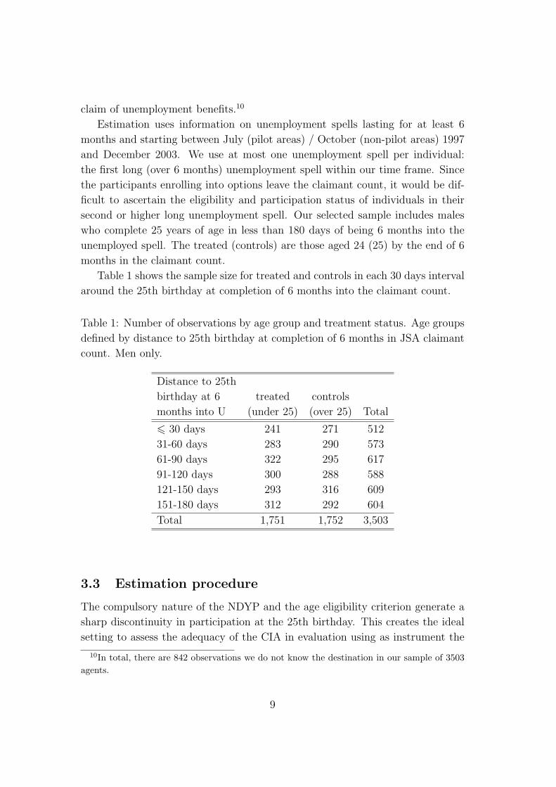
Table 1 shows the sample size for treated and controls in each 30 days interval around the 25th birthday at completion of 6 months into the claimant count.

Table 1: Number of observations by age group and treatment status. Age groups defined by distance to 25th birthday at completion of 6 months in JSA claimant count. Men only.

Distance to 25th birthday at 6 treated controls months into U (under 25) (over 25) Total

� 30 days 241 271 512 31-60 days 283 290 573 61-90 days 322 295 617 91-120 days 300 288 588 121-150 days 293 316 609 151-180 days 312 292 604 Total 1,751 1,752 3,503

3.3 Estimation procedure

The compulsory nature of the NDYP and the age eligibility criterion generate a sharp discontinuity in participation at the 25th birthday. This creates the ideal setting to assess the adequacy of the CIA in evaluation using as instrument the

10In total, there are 842 observations we do not know the destination in our sample of 3503 agents.

9

distance in days to the 25th birthday at completion of 6 months in unemployment. In the evaluation exercise, we consider two alternative outcomes (Y ):

• the re-employment probability 120 days after enrollment, by the end of the tenth month after becoming a claimant or

• the probability of having left the JSA claimant count 120 days after enroll­

ment, by the end of the tenth month after becoming a claimant.

We compare two alternative estimation methods in trying to identify the average impact of treatment on the treated (ATT). The first is the standard matching on the propensity score. The second is the regression discontinuity exploring the sharp design in age.

The matching estimates use the whole sampled population of treated/controls as described above (24 and 25 years old males at less than 180 days of their 25th birthday on completion of 6 months in the claimant count). The propensity score is based on all the observed demographic information and a detailed unemploy­

ment history constructed from the historical records in JUVOS. The covariates used in matching are marital status, region at 2 digits level (37 regions), usual occupation at 2 digits level (77 categories), claiming history over the past 3 years and quarter of inflow. We also single out region to produce a second set of estimates based on propensity score matching coupled with exact matching on region. The matching procedure uses Epanechnikov kernel weights and different bandwidths have been tried.

Figure 1 plots the pdf of the predicted propensity scores for treated and con­

trols using the full specification.11 The two distributions overlap for most of the domain. In fact, the observables are nearly balanced across the two groups even before matching on the propensity score, with a maximum bias of 8%. Matching improves the balancing over half of the observables, namely the ones exhibiting larger bias, without damaging the balance of the remaining observables. In the estimation we exclude observations scoring below the maximum 5 centile and above the minimum 95 centile of the two distributions. This amounts to con­

sidering the central part of the distribution, grossly corresponding to propensity scores above 0.35 and below 0.65.

The regression discontinuity estimates explore further the age-cutoff point for eligibility. We use the same kernel weights as for the matching procedure de­

scribed above. Such weights are then combined with the kernel (Epanechnikov) weights for the distance to 25th birthday at completion of 6 months in unem­

ployment. As we vary the bandwidth on the distance to the 25th birthday, this 11Estimates of the propensity score can be found in Table 8 in the Appendix.

10

Figure 1: Probability density functions: propensity score by treatment status

01

23

45

0 .2 .4 .6 .8propensity score

control group treatment group

corresponds effectively to changing the treatment and control groups. We con­

sider multiples of 30 days for the bandwidth on the distance to the 25th birthday, from 60 to 180 days.12 We then use local linear regressions (LLR) based on two linear models, separately for treated and controls, of the outcome of interest on the distance to the 25th birthday at 6 months into the unemployment spell. Es­

timation is by weighted least squares using the weights described above. The estimated impact is the difference between the intercepts in the two regressions, when the distance to the 25th birthday at 6 months in unemployment is zero.

3.4 Results

We estimate the impact of the NDYP on the two outcomes of interest, namely exits into all destinations and exits into employment within 120 days of joining the program.13 Results for the ATT using exact matching on region are displayed in table 2.

Column 1 in table 2 shows estimates of the impact of treatment on the prob­

ability of leaving the claimant count with 120 days of joining the NDYP and column 2 presents the respective standard errors. According to the discontinuity design estimates in rows 1 to 5, the NDYP seems to have had a positive and

12Comparisons using only individuals at less than 30 days of completing 25 at becoming unemployed for 6 months are very imprecise given the sample size.

13These estimates are based on exact matching on region and a bandwidth of 0.1 for the matching on the propensity score. Estimates using matching on the propensity score only and alternative bandwidths show the same patterns and are available from the authors under request.

11

Table 2: ATT: Impact of the NDYP on the odds of leaving unemployment and finding a job within 120 days of completing 6 months in the claimant count (conditional on having completed 6 months in unemployment); men only

Max dist to 25th btday Exits to all destinations Exits to employment at 180 days into U est se diff(*) se est se diff(�) se

(1) (2) (3) (4) (5) (6) (7) (8)

Regression discontinuity (1) ± 60 days 0.183* 0.081 0.044 0.078 0.123* 0.075 0.073 0.071 (2) ± 90 days 0.180* 0.064 0.040 0.060 0.084* 0.057 0.033 0.053 (3) ± 120 days 0.177* 0.053 0.038 0.049 0.064* 0.049 0.013 0.044 (4) ± 150 days 0.152* 0.048 0.013 0.043 0.072* 0.040 0.021 0.035 (5) ± 180 days 0.143* 0.043 0.004 0.038 0.075* 0.034 0.025 0.029

(6) Simple matching 0.139* 0.020 0.051* 0.018

Notes: The population used in the estimation is defined based on the distance to the 25th birthday on the day 6 months in JSA are completed. We have considered groups up to 180 days away from their 25th birth­

day. The simple matching estimates on the bottom of the table are based on this group using exact matching on region and propensity score matching on the other covariates with kernel weights and a bandwidth of 0.1. Regression-discontinuity estimates use LLR on distance to 25th birthday separately on treated and non-treated using weighted least squares. It then compares the predictions of both regressions at the point where the re­gressor (distance to 25th birthday) is zero to compute the estimated effect. Simple matching differs from the discontinuity design method by not using age information in any more detail than in the definition of the treat­

ment and control groups. Bootstrapped standard errors based on 100 replications. (�) “diff” in columns (3) and (7) refers to the difference between the estimates obtained using regression discon­

tinuity and simple matching. Columns (4) and (8) report the standard errors for the difference obtained using 100 bootstrap replications. * Statistically different from 0 at 5% significance level.

sizeable impact on the probability of leaving unemployment and the estimate becomes larger the closer we get to the cutoff point (25th birthday at inflow into the NDYP). The matching estimator also suggests a positive and large impact on the odds of leaving unemployment but the estimated effect is smaller than any of the estimates obtained using regression discontinuity. A possible explana­

tion for this pattern is that older individuals are more strongly affected by the NDYP. We test the importance of these differences in columns 3 and 4. Column 3 presents the difference between the regression discontinuity and the matching estimates. These are systematically positive and monotonically decreasing with the bandwidth on the distance to the 25th birthday. However, column 4 shows that none of these differences is statistically significant.

Columns 5 to 8 in Table 2 show a similar pattern when exits into employment is the outcome of interest. Again, regression-discontinuity estimates are positive

12

and large, although not as large as the estimates of the impact on the probabilities of leaving unemployment. The matching estimate is equally positive but smaller than any of the discontinuity design estimates. This makes the differences in column 7 systematically positive and higher for the older participants, but again none of these differences is statistically significant.

The evidence in this example does not reject the hypothesis that matching and discontinuity design are estimating the same parameter. But this may be a consequence of the relatively small sample size and how it affects precision, as the estimates do insinuate that differences may exist between the two sets of estimates. Under the discontinuity design assumptions, such differences could arise through two channels. First and more obvious, the regression-discontinuity assumptions do not imply the matching assumptions.14 If, in particular, the conditional independence assumption fails to hold then matching will not identify the ATT. And second, the impact of treatment may vary with age, in which case the eligibility rule effectively creates selection on the potential gains. Such selection does not affect the ability of matching to identify the ATT as only selection on the unobserved part of Y 0 needs to be ruled out. However, selection on potential gains correlated with the instrument implies that the discontinuity design will identify a local parameter, namely the impact of treatment on the treated close to the cutoff point, while matching identifies the global impact of treatment on the treated being considered in the evaluation procedure.

To investigate the importance of heterogeneous treatment effects by age in our application, we compute the age effects using a comparison between 23 and 24 years old males at the enrollment point. Under the matching and discontinuity design assumptions, any non-zero estimates can only be caused by changes in mean gains with age as both groups are to become treated by the NDYP. Table 3 displays the results. All estimates are small and insignificant, independently of the outcome of interest (exits to all destinations - columns 1 and 2 - or exits into employment - columns 3 and 4) and the estimation method (discontinuity design - rows 1 to 5 - or matching - row 6). It is also much less clear from this table that the effects change systematically in the same direction as we include

14We assume that regression discontinuity is valid under the matching conditional indepen­dence assumption. This is generally true. To see why, let Z be the instrument (age) and X be the other covariates used to perform matching, D the treatment status indicator and Y0 be the outcome if the agent is not treated. Now suppose that the regression discontinuity assumption does not hold so that E(Y0|X, Z) has a discontinuity at the threshold in Z, in this example the 25th birthday. But Z univocally determines D and so E(Y0|X, D) will not, in general, be invariant with D, except maybe for very particular groups where the discontinuity is leveled out with observations further away from the cutoff point.

13

Table 3: Age effect: Impact of age on the odds of leaving unemployment and finding a job within 120 days of completing 6 months in the claimant count (conditional on having completed 6 months in unemployed); men aged 23 and 24 only

Exact matching on region Exits to all Exits to

Max dist to 24th btday destinations employment at 180 days into U est se est se

(1) (2) (3) (4)

Regression discontinuity (1) ± 60 days 0.031 0.057 0.032 0.059 (2) ± 90 days 0.012 0.050 0.007 0.046 (3) ± 120 days 0.026 0.044 0.020 0.041 (4) ± 150 days 0.011 0.038 0.008 0.039 (5) ± 180 days -0.002 0.034 -0.006 0.038

(6) Simple matching 0.011 0.016 0.008 0.017

Notes: The population used in the estimation is defined based on the distance to the 24th birthday on the day 6 months in JSA are completed. We have considered groups up to 180 days away from their 24th birthday. The simple matching estimates on the bottom of the table are based on this group using exact matching on region and propensity score matching on the other covariates with kernel weights and a bandwidth of 0.1. Regression-discontinuity estimates use LLR on distance to 24th birthday separately on 23 and 24 years old using least squares with matching weights. It then compares the predictions of both regressions at the point where the regressor (distance to 24th birthday) is zero to compute the estimated effect. Simple matching differs from the discontinuity-design method by not using age information in any more detail than in the definition of the treatment and control groups. Bootstrapped standard errors based on 100 replications.

groups further away from the cutoff point although the estimates in row 1 are still higher than any of the other estimates. In all, however, this table offers no indication of possible age effects.

4 Evaluation of Youth Practice

4.1 The program

Youth Practice (YP) is a Swedish large-scale subsidized-work program targeted at the 18-24 years old unemployed. This program was launched in July 1992. In October 1995 it was subsumed into an extended policy program for youth unemployment. Officially, eligibility required a minimum unemployment duration

14

of 4 months for the 20-24 years old and 8 weeks for the 18-19 years old. We restrict attention to the 20-24 years old because of a range of differences with the policy regime for those below 20 (see Forslund and Nordstrom Skans, 2006, and the other references in Section 1, for details on YP and youth unemployment in Sweden). Participation was not compulsory. In fact, YP was one among several non-compulsory treatments that agents could enter. The most relevant other possible treatment is Labor Market Training, which is an expensive program that mostly consists of vocational training.

The YP program was primarily intended for individuals with a high school diploma. Participants were placed in a job in the private or public sector for 6 months with a possible extension to 12 months. In fact, eligible individuals were encouraged to find such a subsidized job themselves. While at work, participants received an allowance below the current wage rate. The employer paid at most a small fraction of the allowance. The job was supposed to be supplementary in the sense that it should not displace regular employment. In addition to work, the participant was also supposed to spend at least four hours per week at the employment office to search for more regular employment. However, the no-

displacement and the job-search requirement seem to have been violated regularly. Empirical data show that the eligibility requirement concerning the 4-month

minimum unemployment duration was not respected: 28% of participants enter within 30 days of starting a new unemployment spell, and 68% enter before com­

pleting 120 days in unemployment. The age eligibility rule, however, is strictly respected: participants are always below the age of 25 at the moment of enrolling into YP.

4.2 Data

We use the Swedish unemployment register called Handel. This is an adminis­

trative dataset that comprises information from August 1991 onwards on unem­

ployment spells, program participation spells and the subsequent labor market status of those who are deregistered (e.g. employment, education, inactivity or ‘lost’ (attrition)). All individuals with unemployment claiming spells since 1991 are reported in the dataset and their unemployment history can be followed over time. Handel also includes demographic information on age, gender, citizenship, area of residence and education.

For the purposes of our evaluation, we use only the first unemployment spell starting between July 1992 and September 1995, while YP was offered. In the estimation procedure we explore age as the source of randomization by comparing

15

two closely aged groups: those aged 24 with those aged 25 at unemployment inflow. Our analysis is for men only.

The sample size by eligibility and treatment status for different age groups is displayed in Table 4. Each individual is represented only once in our sample as we only consider the first observed unemployment spell within the July 1992 to September 1995 time frame.

Table 4: Number of observations by age group eligibility/treatment status; age groups defined by distance to 25th birthday at inflow into first unemployment spell between July 1992 and October 1995; men only.

ineligibles eligibles (under 25) Distance to 25th birthday (over 25) non-participants participants Total at inflow into U (1) (2) (3) (4)

(1) up to 90 days 7,163 6,915 138 14,367 (2) 91-180 days 7,238 6,447 633 14,535 (3) 181-270 days 7,281 6,145 1,109 14,318 (4) 271-360 days 7,252 5,988 1,227 14,216 (5) Total 28,934 25,455 3,107 57,436

Notes: The population is that of males flowing into unemployment between July 1992 and September 1995 while aged 24 or 25 years old. The participants are taking YP within 360 days of flowing into unemployment without having had another activity (program participation, job or other) since joining the unemployment register.

Column 3 in Table 4 shows that the number of program participants is small even though we use the whole population of treated as recorded in the admin­

istrative unemployment records. The wide availability of alternative treatments may explain why the YP has remained a small program while it lasted. Column 3 in Table 4 also shows that participation is more likely among agents starting unemployment spells further away from their 25th birthday. This is a purely me­

chanical effect: younger agents at inflow into unemployment have more time to participate while eligibles at the verge of completing 25 years of age at inflow have just a few days to enrol into the program. As a consequence, regression disconti­

nuity is not fit to deal with this case. Figure 2 shows how participation changes with age at entrance in unemployment and there is no visible discontinuity to be explored.

We measure the impact of treatment on the odds of leaving unemployment or

16

Figure 2: Probability of participation by age at inflow into unemployment

0.0

5.1

.15

.2.2

5pa

rtic

ipat

ion

rate

22 23 24 25 26age

finding a job after 6, 12, 18 and 24 months of starting the unemployment spell.

4.3 Estimation procedure

Estimation uses the population of males aged 24 or 25 at their first unemployment spell between July 1992 and September 1995. Eligibility is assessed based on age at inflow into unemployment, where those aged 24 are eligibles and those aged 25 are not.

The treated group is composed of the eligibles who select into YP as their first activity after becoming unemployed. We consider alternative treatment groups depending on two dimensions:

1. duration of unemployment prior to enrollment into the YP: up to 0 (many individuals flow straight into YP from employment), 30, 90, 180 and 360 days;

2. and distance in days to 25th birthday at inflow into unemployment - up to 180 and 360 days.15

The control group is composed of eligibles and ineligibles not enrolling into YP as their first activity within the considered time window. The precise definition of control group matches that of the treated group in terms of age and allowed duration of unemployment prior to enrollment into treatment. Notice that we do not require controls to be under 25 at inflow (eligible) as this instrument

15We chose not to tighten this requirement given the small number of treated observations close to the age cutoff point (see Table 4 and discussion above).

17

is used to test the adequacy of matching. We also do not require controls to remain unemployed and untreated for the length of time the treated take to enrol into treatment. This would demand the use of a dynamic framework which has problems of its own and is outside the scope of this study (e.g. Sianesi, 2004, Fredriksson and Johansson, 2008, and De Luna and Johansson, 2007, deal explicitly with dynamic enrolling decisions).

The standard matching estimates are produced using propensity score match-

ing with kernel Epanechnikov weights. The propensity score is estimated on all observable characteristics excluding age, the selected instrument, namely citizen-

ship, education, region of residence, quarter of entry and labor market history in the two years preceding the start of the unemployment spell.

Estimates of the propensity score when individuals are allowed a whole year to enrol into treatment can be found in the Appendix, Table 9. Figure 3 plots the distribution of the predicted scores by treatment and eligibility status for the same sample.

Figure 3: Probability density functions: propensity score

05

1015

dens

ity

0 .1 .2 .3Pr(treat)

treated non−treated

Distribution of the propensity score by treatment status

05

1015

dens

ity

0 .1 .2 .3Pr(treat)

eligibles non−eligibles

Distribution of the propensity score by eligibility status

Enrollment into treatment seems to be partly dependent on the observable characteristics but eligibles and ineligibles as defined by age at inflow are vir­

tually indistinguishable with respect to the distribution of the propensity score. This is also true when the treated are excluded from the group of eligibles as they are a relatively small proportion of this group. In fact, the covariates are relatively balanced between the treated and alternative non-treated groups, even before matching, with a maximum bias of 22%. Matching on the propensity score succeeds in improving balancing for all observables, reducing the bias by about half of its original level in most cases.

Estimation of the correction term requires two alternative control groups. We use the control group just defined above plus the alternative group of ineligibles

18

only. Age is the instrument and the 25th birthday is the cutoff point.16 Alterna­

tive definitions of ineligibles are used to match the definition of treatment group, depending on the distance in days to the 25th birthday. We then match treated with ineligibles using standard kernel matching with Epanechnikov weights and used the matched sample to estimate the additional moment required to compute the correction term, namely the expected value of non-treated outcomes among non-treated ineligibles.

4.4 Results

In what follows we discuss the results for the sample of agents flowing into un­

employment within 360 days of their 25th birthday. Results for other tighter age groups are similar to the ones we present here.

Table 5 describes the number of observations used in estimation. Enrollment into treatment is much more likely at the beginning of the unemployment spell. This is in part a consequence of the definition of treatment used in this paper as being the first program the individual participates in during the unemployment spell. However, participation is a relatively rare event and so the number of participants that move straight into YP from outside unemployment is low. We therefore choose to discuss the impact of participating in YP within 90 and 180 days of inflow into unemployment.

Table 5: Sample size by treatment status and definition of treatment; males completing 25 years of age within 360 days of moving into unemployment

Definition of controls treatment treated eligibles ineligibles

treated within 0 days of inflow into U 601 27,901 28,934 treated within 30 days of inflow into U 1,125 27,377 28,934 treated within 90 days of inflow into U 2,017 26,485 28,934 treated within 180 days of inflow into U 2,911 25,591 28,934 treated within 360 days of inflow into U 3,107 25,395 28,934

Table 6 displays the estimates of the ATT on the probability of finding a job with 12 and 24 months of inflowing into unemployment.

16Age is used to define the eligibility status and to select the working sample only.

19

� �

Table 6: YP: ATT on the outflows to employment; men aged 24 or 25 at inflow into unemployment

Days between becoming Average outcome ATT correction ATT unemployed and treated controls (st matching) term (corrected) enrolling into treatment (1) (2) (3) (4) (5)

Outcome: finding a job within 12 months of becoming unemployed (1) less than 90 0.332 0.335 -0.002 0.049 -0.052

(0.010) (0.062) (0.063) (2) less than 180 0.320 0.330 -0.010 0.028 -0.038

(0.010) (0.041) (0.041) Outcome: finding a job within 24 months of becoming unemployed

(3) less than 90 0.468 0.437 0.030* 0.099** -0.069 (0.013) (0.060) (0.063)

(4) less than 180 0.450 0.436 0.014 0.069 -0.055 (0.010) (0.048) (0.049)

Notes: Estimates for male aged 24 or 25 years old when enrolling into unemployment. Eligibility to YP depends on age at inflow: unemployed agents are eligibles (ineligibles) if have not (have) completed 25 years of age on the day they register as unemployed. “Treatment” means “enrolling into YP as the first program during the unemployment spell within some time of becoming unemployed”. We have considered alternative time windows for the duration of unemployment prior to treatment, namely 90 (rows 1 and 3) and 180 days (rows 2 and 4). The impact of treatment is estimated on the probability of finding a job within 12 months (rows 1 and 2) and 24 months (rows 3 and 4) of becoming unemployed. Matching is performed on the propensity score using Epanechnikov kernel weights with a bandwidth of 0.06. Bootstrapped standard errors based on 100 replications in brackets below the estimate. * Statistically different from zero at 5% significance level. ** Statistically different from zero at 10% significance level.

Column 3 on the table presents the standard matching estimates of the im­

pact of YP. The estimated effect is small and statistically insignificant in all cases except for the exits into employment within 24 months of inflow for those being treated early in their unemployment spell (within 90 days of becoming unem­

ployed - row 3). In this case, matching suggests that the program improves the odds of finding a job by 3 percent. The correction terms in column 4 are also not significantly different from zero in all but the same case as above, in which case there is some evidence of it being statistically different from zero. Moreover, the correction terms are systematically positive and considerably higher in ab­

solute terms than the estimated effects. As a consequence, all corrected effects become negative (column 5) although none is statistically different from zero at conventional significance levels.

20

� �

Table 7: YP: ATT on the outflows to all destinations; men aged 24 or 25 at inflow into unemployment

Days between becoming Average outcome ATT correction ATT unemployed and enrolling treated controls (st matching) term (corrected) into treatment (1) (2) (3) (4) (5)

Outcome: leaving unemployment within 12 months of becoming unemployed (1) less than 90 days 0.460 0.512 -0.052* -0.078 0.026

(0.013) (0.062) (0.062) (2) less than 180 days 0.438 0.511 -0.073* -0.104* 0.031

(0.011) (0.046) (0.048) Outcome: leaving unemployment within 24 months of becoming unemployed

(3) less than 90 days 0.668 0.645 0.022** -0.070 0.092** (0.013) (0.053) (0.054)

(4) less than 180 days 0.639 0.646 -0.007 -0.077 0.071 (0.011) (0.053) (0.054)

Notes: Estimates for male aged 24 or 25 years old when enrolling into unemployment. Eligibility to YP depends on age at inflow: unemployed agents are eligibles (ineligibles) if have not (have) completed 25 years of age on the day they register as unemployed. “Treatment” means “enrolling into YP as the first program during the unemployment spell within some time of becoming unemployed”. We have considered alternative time windows for the duration of unemployment prior to treatment, namely 90 (rows 1 and 3) and 180 days (rows 2 and 4). The impact of treatment is estimated on the probability of leaving unemployment within 12 months (rows 1 and 2) and 24 months (rows 3 and 4) of becoming unemployed. Matching is performed on the propensity score using Epanechnikov kernel weights with a bandwidth of 0.06. Bootstrapped standard errors based on 100 replications in brackets below the estimate. * Statistically different from zero at 5% significance level. ** Statistically different from zero at 10% significance level.

Table 7 shows similar estimates when outflows into all destination is the out­

come of interest. In this case the standard matching suggest that YP affects negatively the odds of leaving unemployment within 12 months of starting, pos­

sibly detecting some lock-in effect (column 3, rows 1 and 2). The treatment effects on the probability of leaving unemployment within 24 months of entering become positive or zero, which is also consistent with the lock-in interpretation (column 3, rows 3 and 4). However, the correction term is now always negative and again larger in absolute terms than the treatment effect but generally not statistically significant with one exception (column 4). As a consequence, the corrected estimates are always positive or zero and apparently increasing with time from entry into unemployment.

Overall, both tables suggest that matching may not be identifying the correct

21

parameter although the evidence is not conclusive. Possibly, precise estimates of corrected effects require a higher take-up rate than what is found in the YP (see figure 3 for the distribution of the predicted probability of participation). Since the denominator of the correction term is the program take-up rate, by being small it introduces significant variability in the estimated correction terms and corrected treatment effects.

5 Discussion of empirical evaluation results

The British NDYP and the Swedish YP have been evaluated before, as well as a large number of other labor market programs throughout Europe. We briefly compare our results to the existing literature.

In the past, youth programs have often shown disappointing results. Heck­

man, LaLonde and Smith (1999) survey a large number of evaluation studies on US and European programs. Results for the US suggest that labor market programs may have no impact or even a negative impact on the employment probability and wages of young people. European interventions seem to have been more successful in improving the employment prospects and wages of the treated. The disparity of results may be a consequence of differences in program design and/or population of treated. Labor market programs in Europe tend to be larger, more generous and to reach a wider, more heterogeneous population than those in the US. The incidence of unemployment is much lower in the US, and programs in the US are often specifically designed to focus on the very disad­

vantaged. Conceivably, these may not be as ready to benefit from treatment and may face a stronger stigma from treatment than their European counterparts. More recently, Kluve (2006)’s survey of the evaluation results in Europe finds that young men do not seem to benefit from these interventions in terms of labor market outcomes, while young women are found to benefit more frequently.

The British NDYP has been the focus of several evaluation studies (e.g. Blun­

dell et al., 2004, De Giorgi, 2005). On a more optimistic note, results have consis­

tently shown significant positive effects of the program on the employment prob­

abilities of young males. All studies compare unemployed completing 6 months in the claimant count. In one set of estimates, Blundell et al. (2004) explore the age threshold rule within matching coupled with difference-in-differences to estimate the impact of the NDYP on the probability of finding a job within 10 months of flowing into unemployment. De Giorgi (2005) uses regression discontinuity in age with a bandwidth close to 180 days to measure the impact of the NDYP on the probability of employment 18 months after the start on the unemployment

22

spell. His estimates suggest that the program has improved the chances of em­

ployment among the treated by 5-7%, and are in line with those in Blundell et al. (2004) and our own for a similar bandwidth (row 5 and column 5 in table 2). These results suggest that the mixture of improved job-search assistance and tougher job-search monitoring used in the NDYP has helped moving and keeping young unemployed out of subsidies in the UK. While it is unclear which of the two mechanisms played the most important role, evidence from other European countries also hint that such combination may work (Anderson, 2000, Van den Berg et al., 2004, and Van den Berg and Van der Klaauw, 2006, and references therein). In terms of our comparison between matching and discontinuity design, the results of the three studies taken together further support the claim that the careful use of matching in the evaluation of the NDYP has identified the true ATT treatment effect parameter.

Swedish subsidized work programs have also been the focus of several studies. Sianesi (2004) carefully analyzes the overall impact of the Swedish ALMP system and the differential impact of each of the numerous available treatments for adults (so this excludes YP). She finds that subsidized employment is the best performer in terms of moving unemployed back into work, and that the positive effect of subsidized employment seems to last. All other programs have either a zero or a negative impact, possibly arising through the renewed eligibility to benefits as a consequence of program participation. The pivotal YP evaluation is in Larsson (2003). In contrast to Sianesi’s results for adults, Larsson finds strong negative effects of this program on the probability of leaving unemployment within 12 months of treatment, that then fade to zero after 24 months. These results are more pessimistic than our own although not completely incompatible. Possibly explaining the differences is the fact that Larsson constructs a comparison group conditional on not being treated for the whole duration of the treatment spell. But, to put it extreme, this effectively amounts to conditioning on a successful outcome, especially in the Swedish system where the decision is between partici­

pating now against waiting a little longer while trying to find a job. As has been widely reported in studies of the Swedish system (see e.g. Larsson, 2003), those who stay unemployed long enough will eventually participate in one of the many treatments available. If an unemployed individual is observed not to participate in a treatment, then this may be to some extent because they manage to leave unemployment before participation.

Our results suggest that YP has no impact on employment outcomes but may, in the longer run (after 24 months) lead to (probably temporary) exit from unem­

ployment for other reasons. For example, individuals may move into education or

23

take further treatment (possibly cycling between open unemployment and treat­

ment to take advantage of the possibility to renew eligibility to unemployment benefits through treatment participation).

6 Conclusion

We have developed and applied an evaluation method for the effects of program participation (or policy exposure) on individual outcomes, if participation is se­lective but individuals are ineligible in case of a certain value of some observed instrumental variable. From a practical point of view this is a common setting, in particular for active labor market policies for young individuals. In those cases, participation may be selective because individuals can choose between different programs and/or because the duration until enrollment is not deterministically set. Program participation is only possible if the individual is aged below a cer­tain age. With selective participation, if the CIA is violated, matching cannot be used. For the same reason, one cannot simply compare those below the threshold who are treated to those above the threshold (who are all non-treated). How­

ever, our novel method, which exploits the eligibility boundary restriction within the matching framework, provides consistent estimates of the average treatment effect on those who are treated.

Our approach relies critically on the availability of an instrument satisfying assumptions 1 and 2 in section 2. Assumption 2 is automatically satisfied in our preferred practical application of a policy that allows for selective participation only on certain values of an observed variable. To obtain precise estimates of our correction term, however, we also require the program to generate a reasonable number of participants.

The application to the Swedish Youth Practice program shows that our method can deliver evaluation results that differ from those based on standard matching methods. The matching estimates for the effect on re-employment are sometimes significantly positive, whereas the estimates based on our method are always in­

significant. The difference between the estimates is sometimes significant. The re-employment effects are invariably estimated to be smaller than those based on matching, whereas for the effects on the over-all exit probabilities out of unem­

ployment the reverse holds. As a result, we are less optimistic about the effect of subsidized work on the rate of finding work than if we had incorrectly based ourselves on the matching estimates, and we are more optimistic concerning the transition rate to other destinations. From a policy point of view, our results suggest that perhaps an optimism about the use of subsidized work programs to

24

bring unemployed youth back to work should be tempered. An additional contribution of the paper concerns the performance of the

matching method in the case of a sharp eligibility-discontinuity design. Specifi­

cally, we examine this for the New Deal for Young People program for unemployed youth aged below 25. It turns out that matching is able to capture the assign­

ment mechanism, in the sense that the estimates based on matching are not significantly different from those obtained with regression-discontinuity methods.

25

References

Anderson, P. (2000), “Monitoring and Assisting Active Job Search”, OECD Pro­

ceedings, Labour Market Policies and the Public Employment Service

Andrews, D. and M. Schafgans (1998) “Semiparametric Estimation of the Inter­

cept of a Sample Selection Model,” Review of Economic Studies, 65, 497–517

Angrist, J.D, and G.W. Imbens (1991), “Sources of Identifying Information in Evaluation Models”, Working Paper, NBER. Cambridge MA

Battistin, E. and E. Rettore (2007), “Ineligibles and Eligible Non-Participants as a Double Comparison Group in Regression Discontinuity Designs”, Journal of Econometrics, forthcoming

Blundell, R., M. Costa Dias, C. Meghir and J. Van Reenen (2004), “Evaluating the Employment Impact of a Mandatory Job Search Program”, Journal of the European Economic Association, 2(4), 569–606

Bonnal, L., D. Fougere, and A. Serandon (1997), “Evaluating the Impact of French Employment Policies on Individual Labour Market Histories,” Review of Economic Studies, 64, 683–713

Burgess, S., C. Propper, H. Rees and A. Shearer (2003), “The Class of 1981: The Effects of Early Career Unemployment on Subsequent Unemployment Experiences”, Labour Economics, 10, 291–309

Card, D. and D. Sullivan (1988), “Measuring the Effect of Subsidized Training Programs on Movements in and out of Employment,” Econometrica, 56, 497– 530

Cochrane, W. and D. Rubin (1973), “Controlling Bias in Observational Studies,” Sankyha, 35, 417–446

De Giorgi, G. (2005), “Long-term effects of a mandatory multistage program: the New Deal for Young People in the UK”, Working paper, IFS, London

De Luna, X. and P. Johansson (2007), “Matching estimators for the effect of a treatment on survival times”, Working paper, IFAU. Uppsala

Dorsett, R. (2006) “The new deal for young people: effect on the labour market status of young men”, Labour Economics, 13, 405–422

DWP (2006), Departmental Report 2006, Working paper, Department for Work and Pensions, London

Forslund, A. and O. Nordstrom Skans (2006), “Swedish youth labour market policies revisited”, Working paper, IFAU, Uppsala

26

Fredriksson P. and P. Johansson (2008), “Dynamic Treatment Assignment - The Consequences for Evaluations using Observational Data”, Journal of Business and Economics Statistics, forthcoming

Gritz, R. (1993), “The Impact of Training on the Frequency and Duration of Employment,” Journal of Econometrics, 57, 21–51

Heckman, J., H. Ichimura, and P. Todd, (1998) “Matching as an Econometric Evaluation Estimator,” Review of Economic Studies, 65, 261–294

Heckman, J., H. Ichimura, J. Smith, and P. Todd (1998) “Characterization of Selection Bias Using Experimental Data,” Econometrica, 66, 1017–1098

Heckman, J., R. LaLonde and J. Smith (1999), “The Economics and Economet­

rics of Active Labor Market Programs” in O. Ashenfelter and D. Card (eds.), Handbook of Labor Economics, Volume 3, 1865-2097

Heckman, J. and R. Robb (1985) “Alternative Methods for Evaluating the Impact of Interventions,” in J. Heckman and B. Singer (eds.), Longitudinal Analysis of Labor Market Data, Cambridge University Press, New York

Kluve, J. (2006), “The Effectiveness of European Active Labor Market Policy”, Working paper, RIW, Essen

LaLonde, R. (1986), “Evaluating the Econometric Evaluations of Training Pro­

grams with Experimental Data,” American Economic Review, 76, 604–620

Larsson, L. (2003), “Evaluation of Swedish Youth Labor Market Programs”, Journal of Human Resources, 38, 891–927

Layard, R. (2000), “Welfare to Work and the New Deal”, The Business Economist, 31(3), 28–40

Richardson, K. and G.J. van den Berg (2001), “The Effect of Vocational Em­

ployment Training on the Individual Transition Rate from Unemployment to Work,” Swedish Economic Policy Review, 8, 175–213

Rosenbaum, P. and D. Rubin (1983) “The Central Role of the Propensity Score in Observational Studies for Causal Effects,” Biometrika, 70, 41–55

Sianesi, B. (2004), “An Evaluation of the Swedish System of Active Labour Market Programmes in the 1990s”, Review of Economics and Statistics, 86, 1, 133–155

Van den Berg, G.J., B. van der Klaauw, and J.C. van Ours (2004), “Punitive Sanctions and the Transition Rate from Welfare to Work,” Journal of Labor Economics, 22, 211–241

27

Van den Berg, G.J. and B. van der Klaauw (2006), “Counselling and Monitor­

ing of Unemployed Workers: Theory and Evidence from a Controlled Social Experiment, International Economic Review, 47, 895–936

Van der Klaauw, W. (2008), “Regression-Discontinuity Analysis”, in: S.N. Durlauf and L.E. Blume (eds.), New Palgrave Dictionary of Economics, Palgrave Macmil­

lan, Basingstoke, forthcoming

Van Reenen, J. (2004), “Active Labour Market Policies and the British New Deal for Unemployed Youth in Context”, in R. Blundell, D. Card and R. Freeman (eds.), Seeking a Premier Economy, University of Chicago Press

White, M. and G. Knight (2002), “Benchmarking the effectiveness of NDYP: A review of European and US literature on the microeconomic effects of labour market programmes for young people”, Working paper, PSI, London

28

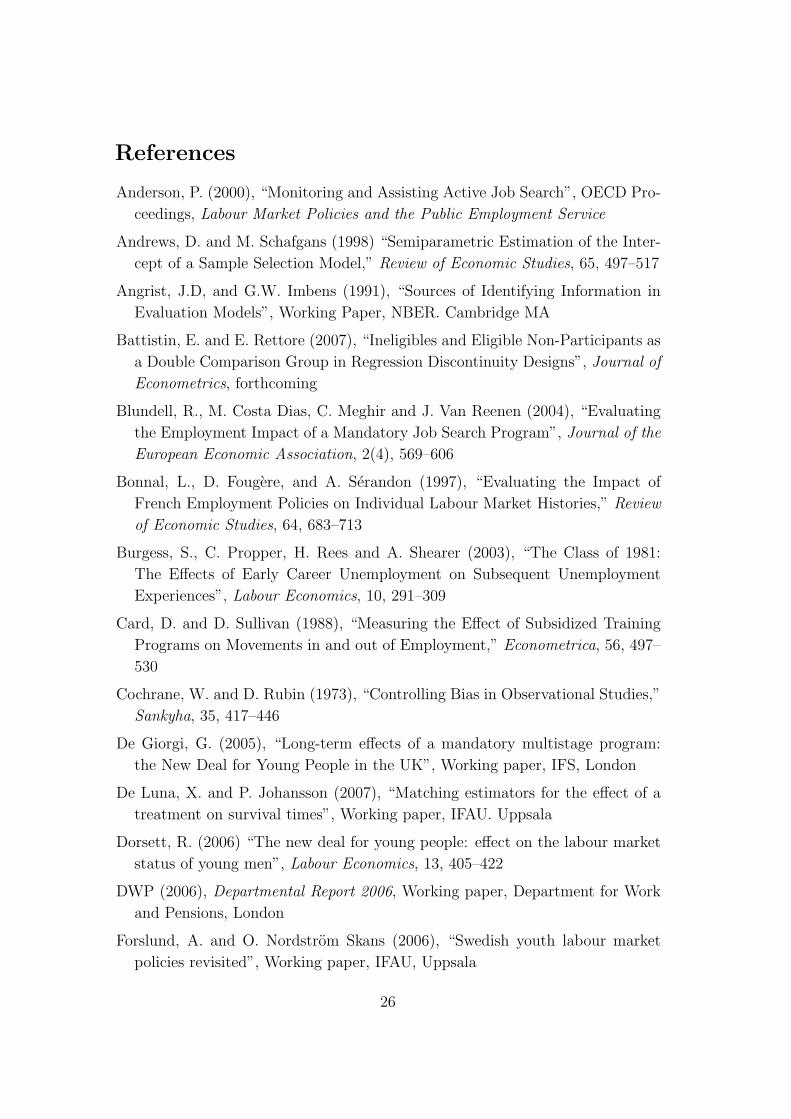
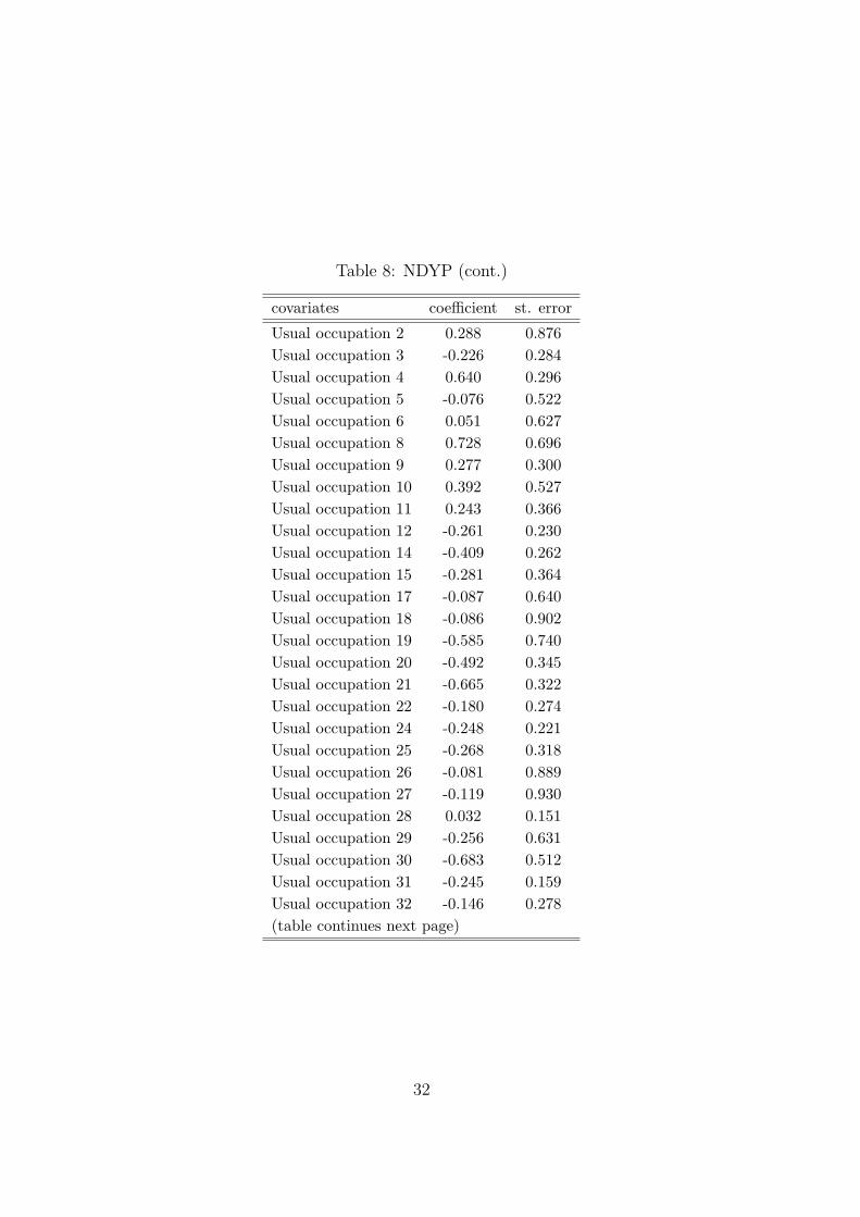
Appendix: Propensity score estimates

Table 8 shows the estimates of the propensity score for the NDYP application. We tested the joint significance of the groups of variables. Only marital status and quarter of entrance are statistically significant. Table 9 displays the estimates of the propensity score for the YP application. Alternative specifications have been tried but do not change the nature of the results in both cases.

Table 8: NDYP (part 1)

covariates coefficient st. error

constant 0.382 0.271

Marital status: married -0.004 0.075 Marital status: divorced/widow -0.397 0.125 Marital status: unknown -0.050 0.097

U spells past year: none -0.169 0.222 U spells past year: 1 -0.154 0.204 U spells past year: 2 -0.097 0.195 U spells past year: 3 -0.116 0.197 U spells past 2 years: none 0.089 0.212 U spells past 2 years: 1 0.211 0.177 U spells past 2 years: 2 0.248 0.154 U spells past 2 years: 3 0.100 0.131 U spells past 3 years: none 0.060 0.168 U spells past 3 years: 1 -0.018 0.137 U spells past 3 years: 2 -0.004 0.119 U spells past 3 years: 3 -0.042 0.104

% time in U past year -0.111 0.186 % time in U past 2 years -0.265 0.321 % time in U past 3 years 0.309 0.266

Inflow in U: 97:IV -0.257 0.203 Inflow in U: 98:I -0.476 0.206 Inflow in U: 98:II -0.364 0.207 Inflow in U: 98:III -0.402 0.207 Inflow in U: 98:IV -0.437 0.209 (table continues next page)

29

Table 8: NDYP (cont.)

covariates coefficient st. error

Inflow in U: 99:I -0.622 0.209 Inflow in U: 99:II -0.433 0.215 Inflow in U: 99:III -0.317 0.213 Inflow in U: 99:IV -0.396 0.219 Inflow in U: 00:I -0.441 0.218 Inflow in U: 00:II -0.572 0.235 Inflow in U: 00:III -0.431 0.222 Inflow in U: 00:IV -0.501 0.225 Inflow in U: 01:I -0.289 0.235 Inflow in U: 01:II -0.408 0.240 Inflow in U: 01:III -0.174 0.243 Inflow in U: 01:IV 0.082 0.247 Inflow in U: 02:I -0.036 0.244 Inflow in U: 02:II -0.268 0.253 Inflow in U: 02:III -0.226 0.238 Inflow in U: 02:IV 0.052 0.248 Inflow in U: 03:I -0.214 0.239 Inflow in U: 03:II -0.099 0.260 Inflow in U: 03:III -0.166 0.249 Inflow in U: 03:IV -0.280 0.246

Region 2 0.039 0.105 Region 3 0.088 0.108 Region 4 0.003 0.114 Region 5 -0.125 0.209 Region 6 0.108 0.211 Region 7 0.216 0.157 Region 8 0.311 0.239 (table continues next page)

30

Table 8: NDYP (cont.)

covariates coefficient st. error

Region 9 0.007 0.166 Region 10 -0.005 0.320 Region 11 0.074 0.117 Region 12 0.098 0.117 Region 13 0.169 0.212 Region 14 0.135 0.222 Region 15 0.038 0.141 Region 16 0.049 0.189 Region 17 0.067 0.195 Region 18 0.806 0.487 Region 19 0.123 0.118 Region 20 0.031 0.107 Region 21 0.247 0.135 Region 22 0.202 0.102 Region 23 0.131 0.171 Region 24 0.646 0.547 Region 26 -0.062 0.217 Region 27 0.270 0.280 Region 28 -0.401 0.337 Region 29 -0.054 0.123 Region 30 0.024 0.244 Region 31 -0.031 0.223 Region 32 0.088 0.135 Region 33 0.088 0.122 Region 34 -0.073 0.155 Region 35 -0.004 0.221 Region 36 0.0587 0.136 (table continues next page)

31

5

10

15

20

25

30

Table 8: NDYP (cont.)

covariates coefficient st. error

Usual occupation 2 0.288 0.876 Usual occupation 3 -0.226 0.284 Usual occupation 4 0.640 0.296 Usual occupation -0.076 0.522 Usual occupation 6 0.051 0.627 Usual occupation 8 0.728 0.696 Usual occupation 9 0.277 0.300 Usual occupation 0.392 0.527 Usual occupation 11 0.243 0.366 Usual occupation 12 -0.261 0.230 Usual occupation 14 -0.409 0.262 Usual occupation -0.281 0.364 Usual occupation 17 -0.087 0.640 Usual occupation 18 -0.086 0.902 Usual occupation 19 -0.585 0.740 Usual occupation -0.492 0.345 Usual occupation 21 -0.665 0.322 Usual occupation 22 -0.180 0.274 Usual occupation 24 -0.248 0.221 Usual occupation -0.268 0.318 Usual occupation 26 -0.081 0.889 Usual occupation 27 -0.119 0.930 Usual occupation 28 0.032 0.151 Usual occupation 29 -0.256 0.631 Usual occupation -0.683 0.512 Usual occupation 31 -0.245 0.159 Usual occupation 32 -0.146 0.278 (table continues next page)

32

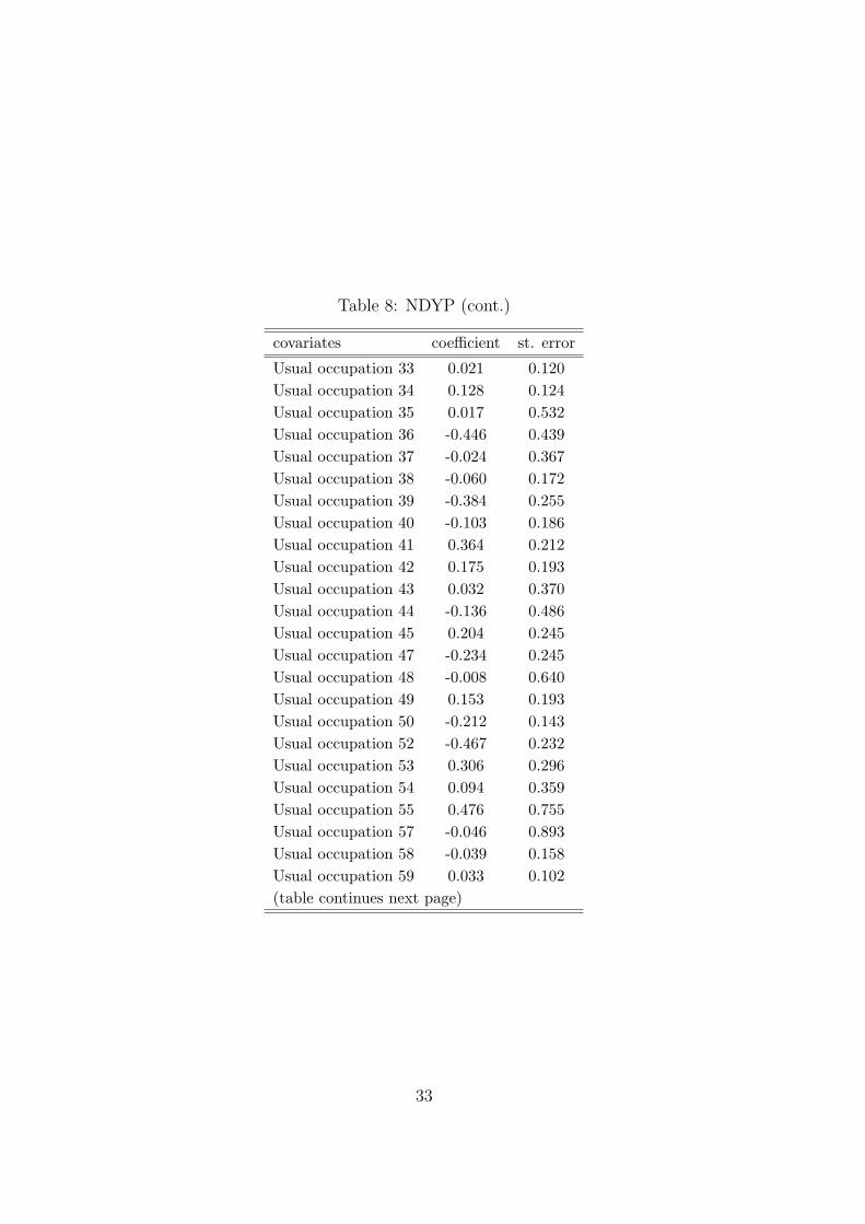
Table 8: NDYP (cont.)

covariates coefficient st. error

Usual occupation 33 0.021 0.120 Usual occupation 34 0.128 0.124 Usual occupation 35 0.017 0.532 Usual occupation 36 -0.446 0.439 Usual occupation 37 -0.024 0.367 Usual occupation 38 -0.060 0.172 Usual occupation 39 -0.384 0.255 Usual occupation 40 -0.103 0.186 Usual occupation 41 0.364 0.212 Usual occupation 42 0.175 0.193 Usual occupation 43 0.032 0.370 Usual occupation 44 -0.136 0.486 Usual occupation 45 0.204 0.245 Usual occupation 47 -0.234 0.245 Usual occupation 48 -0.008 0.640 Usual occupation 49 0.153 0.193 Usual occupation 50 -0.212 0.143 Usual occupation 52 -0.467 0.232 Usual occupation 53 0.306 0.296 Usual occupation 54 0.094 0.359 Usual occupation 55 0.476 0.755 Usual occupation 57 -0.046 0.893 Usual occupation 58 -0.039 0.158 Usual occupation 59 0.033 0.102 (table continues next page)

33

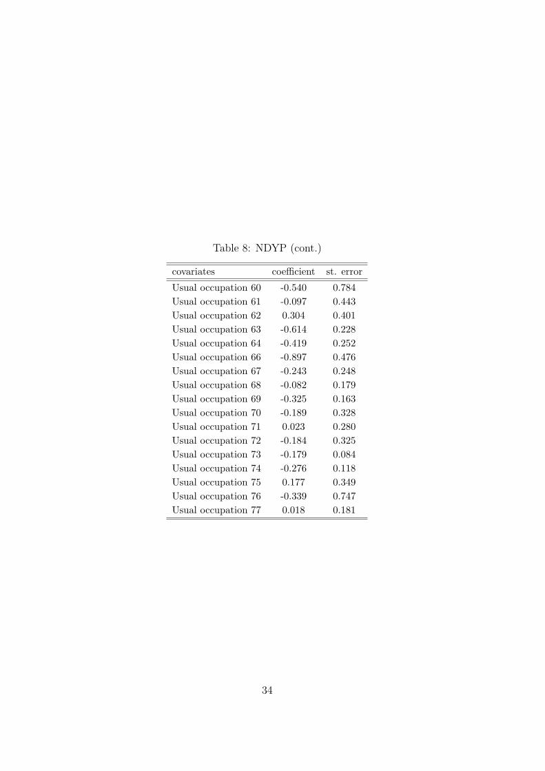
Table 8: NDYP (cont.)

covariates coefficient st. error

Usual occupation 60 -0.540 0.784 Usual occupation 61 -0.097 0.443 Usual occupation 62 0.304 0.401 Usual occupation 63 -0.614 0.228 Usual occupation 64 -0.419 0.252 Usual occupation 66 -0.897 0.476 Usual occupation 67 -0.243 0.248 Usual occupation 68 -0.082 0.179 Usual occupation 69 -0.325 0.163 Usual occupation 70 -0.189 0.328 Usual occupation 71 0.023 0.280 Usual occupation 72 -0.184 0.325 Usual occupation 73 -0.179 0.084 Usual occupation 74 -0.276 0.118 Usual occupation 75 0.177 0.349 Usual occupation 76 -0.339 0.747 Usual occupation 77 0.018 0.181

34

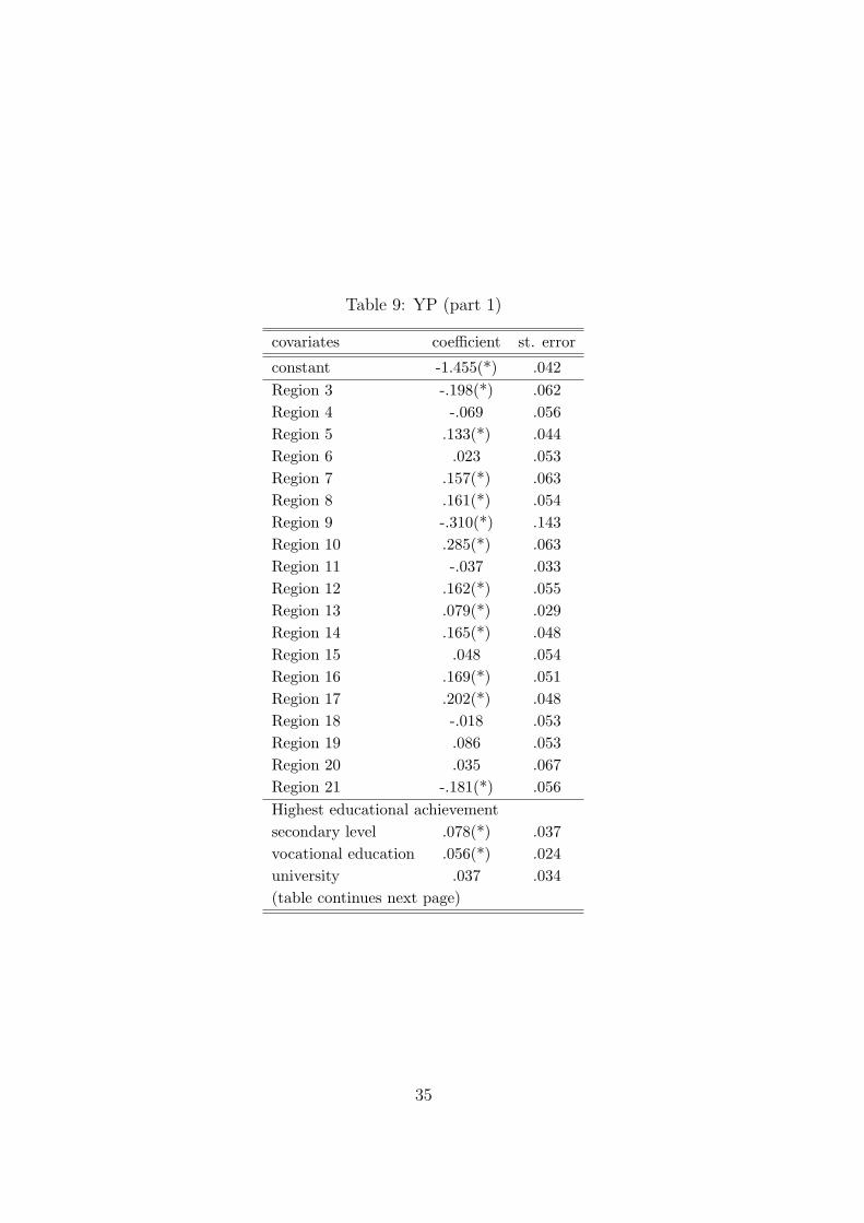
Table 9: YP (part 1)

covariates coefficient st. error

constant -1.455(*) .042

Region 3 -.198(*) .062 Region 4 -.069 .056 Region 5 .133(*) .044 Region 6 .023 .053 Region 7 .157(*) .063 Region 8 .161(*) .054 Region 9 -.310(*) .143 Region 10 .285(*) .063 Region 11 -.037 .033 Region 12 .162(*) .055 Region 13 .079(*) .029 Region 14 .165(*) .048 Region 15 .048 .054 Region 16 .169(*) .051 Region 17 .202(*) .048 Region 18 -.018 .053 Region 19 .086 .053 Region 20 .035 .067 Region 21 -.181(*) .056

Highest educational achievement secondary level .078(*) .037 vocational education .056(*) .024 university .037 .034 (table continues next page)

35

Table 9: YP (cont.)

covariates coefficient st. error

Unemployment history (**) % time in U over last year .258(*) .081 % time in U over last 2 years .170 .106 % time in T over last year .175 .104 % time in T over last 2 years .156 .117 % time in YP over last year .772(*) .188 % time in YP over last 2 years .267 .271 % time in E over last year -.444(*) .216 % time in E over last 2 years .098 .336

Quarter of inflow into unemployment quarter II -.205(*) .031 quarter III -.093(*) .030 quarter IV -.110(*) .032

Year of inflow into unemployment 1993 -.268(*) .027 1994 -.464(*) .035 1995 -1.657(*) .157

Notes: Estimates from a probit regression of the participation dummy variable on all observables except age using 57431 obser­

vations in total. (*) Statistically different from zero at the conventional 5% signifi­

cance level. (**) U stands for unemployment, T stands for treatment other then YP, YP stands for Youth Practice and E stands for employment. Individuals may have had previous YP spells from open unemploy­

ment spells in July 1st, 1992.

36

Publication series published by the Institute for Labour Market Policy Evaluation (IFAU) – latest issues

Rapporter/Reports

2008:1 de Luna Xavier, Anders Forslund and Linus Liljeberg ”Effekter av yrkesinriktad arbetsmarknadsutbildning för deltagare under perioden 2002–04”

2008:2 Johansson Per and Sophie Langenskiöld ”Ett alternativt program för äldre långtids­arbetslösa – utvärdering av Arbetstorget för erfarna”

2008:3 Hallberg Daniel ”Hur påverkar konjunktursvängningar förtida tjänstepensionering?”

2008:4 Dahlberg Matz and Eva Mörk ”Valår och den kommunala politiken”

2008:5 Engström Per, Patrik Hesselius, Bertil Holmlund and Patric Tirmén ”Hur fungerar arbetsförmedlingens anvisningar av lediga platser?”

2008:6 Nilsson J Peter “De långsiktiga konsekvenserna av alkoholkonsumtion under gravi­diteten”

2008:7 Alexius Annika and Bertil Holmlund ”Penningpolitiken och den svenska arbetslös­heten”

2008:8 Anderzén Ingrid, Ingrid Demmelmaier, Ann-Sophie Hansson, Per Johansson, Erica Lindahl and Ulrika Winblad ”Samverkan i Resursteam: effekter på organisation, hälsa

och sjukskrivning”

Working papers

2008:1 Albrecht James, Gerard van den Berg and Susan Vroman “The aggregate labor market effects of the Swedish knowledge lift programme”

2008:2 Hallberg Daniel “Economic fluctuations and retirement of older employees”

2008:3 Dahlberg Matz and Eva Mörk “Is there an election cycle in public employment? Separating time effects from election year effects”

2008:4 Nilsson J Peter ”Does a pint a day affect your child’s pay? The effect of prenatal alcohol exposure on adult outcomes”

2008:5 Alexius Annika and Bertil Holmlund “Monetary policy and Swedish unemployment fluctuations”

2008:6 Costa Dias Monica, Hidehiko Ichimura and Gerard van den Berg ”The matching method for treatment evaluation with selective participation and ineligibles”

Dissertation series

2007:1 Lundin Martin “The conditions for multi-level governance: implementation, politics and cooperation in Swedish active labor market policy”

2007:2 Edmark Karin “Interactions among Swedish local governments”

2008:1 Andersson Christian “Teachers and Student outcomes: evidence using Swedish data”