the mixer module user’s guide - lost-contact.mit.edu ... · example from the mixer module model...

VERSION 4.4

User s Guide

Mixer Module

C o n t a c t I n f o r m a t i o n

Visit the Contact COMSOL page at www.comsol.com/contact to submit general inquiries, contact Technical Support, or search for an address and phone number. You can also visit the Worldwide Sales Offices page at www.comsol.com/contact/offices for address and contact information.

If you need to contact Support, an online request form is located at the COMSOL Access page at www.comsol.com/support/case.

Other useful links include:

• Support Center: www.comsol.com/support

• Product Download: www.comsol.com/support/download

• Product Updates: www.comsol.com/support/updates

• COMSOL Community: www.comsol.com/community

• Events: www.comsol.com/events

• COMSOL Video Center: www.comsol.com/video

• Support Knowledge Base: www.comsol.com/support/knowledgebase

Part number: CM023301

M i x e r M o d u l e U s e r ’ s G u i d e © 1998–2013 COMSOL

Protected by U.S. Patents 7,519,518; 7,596,474; 7,623,991; and 8,457,932. Patents pending.

This Documentation and the Programs described herein are furnished under the COMSOL Software License Agreement (www.comsol.com/sla) and may be used or copied only under the terms of the license agreement.

COMSOL, COMSOL Multiphysics, Capture the Concept, COMSOL Desktop, and LiveLink are either registered trademarks or trademarks of COMSOL AB. All other trademarks are the property of their respective owners, and COMSOL AB and its subsidiaries and products are not affiliated with, endorsed by, sponsored by, or supported by those trademark owners. For a list of such trademark owners, see www.comsol.com/tm.

Version: November 2013 COMSOL 4.4

http://www.comsol.com/sla/

http://www.comsol.com/tm/

http://www.comsol.com/contact/

http://www.comsol.com/contact/offices/

http://www.comsol.com/support/case/

http://www.comsol.com/support/

http://www.comsol.com/support/download/

http://www.comsol.com/support/updates/

http://www.comsol.com/community/

http://www.comsol.com/events/

http://www.comsol.com/video/

http://www.comsol.com/support/knowledgebase/

C o n t e n t s

C h a p t e r 1 : I n t r o d u c t i o n

About the Mixer Module 8

The Mixer Module Interfaces . . . . . . . . . . . . . . . . . . 10

Where Do I Access the Documentation?. . . . . . . . . . . . . . 14

Overview of the User’s Guide 18

Tutorial Example—Non-Isothermal Mixer 19

C h a p t e r 2 : M i x e r M o d u l e T h e o r y

Theory for the Free Surface Features 34

Free Surface Domain . . . . . . . . . . . . . . . . . . . . . 34

Free Surface Conditions . . . . . . . . . . . . . . . . . . . . 35

Contact Angle . . . . . . . . . . . . . . . . . . . . . . . . 35

Rotating Shaft Conditions . . . . . . . . . . . . . . . . . . . 36

References for the Free Surface Features . . . . . . . . . . . . . . 37

C h a p t e r 3 : R o t a t i n g M a c h i n e r y , F l u i d F l o w

The Rotating Machinery, Fluid Flow Interfaces 40

The Rotating Machinery, Laminar Flow Interface . . . . . . . . . . . 40

The Rotating Machinery, Turbulent Flow, k- Interface . . . . . . . . . 42

The Rotating Machinery, Turbulent Flow, k- Interface . . . . . . . . 43

The Rotating Machinery, Turbulent Flow, Low Re k- Interface . . . . . 44

Domain, Boundary, Point, and Pair Nodes for the Rotating

Machinery, Laminar and Turbulent Flow Interfaces . . . . . . . . . 45

Initial Values. . . . . . . . . . . . . . . . . . . . . . . . . 46

Rotating Domain . . . . . . . . . . . . . . . . . . . . . . . 46

Rotating Wall . . . . . . . . . . . . . . . . . . . . . . . . 47

C O N T E N T S | 3

4 | C O N T E N T S

Rotating Interior Wall . . . . . . . . . . . . . . . . . . . . . 48

Free Surface Domain . . . . . . . . . . . . . . . . . . . . . 49

Free Surface. . . . . . . . . . . . . . . . . . . . . . . . . 49

Contact Angle . . . . . . . . . . . . . . . . . . . . . . . . 50

Navier Slip . . . . . . . . . . . . . . . . . . . . . . . . . 51

Rotating Shaft . . . . . . . . . . . . . . . . . . . . . . . . 51

C h a p t e r 4 : R o t a t i n g M a c h i n e r y , N o n - I s o t h e r m a l

F l o w

The Rotating Machinery, Non-Isothermal Flow Interfaces 54

Rotating Machinery, Non-Isothermal Flow, Laminar Flow Interface . . . . 54

Rotating Machinery, Non-Isothermal Flow, Turbulent Flow, k- Interface. . . . . . . . . . . . . . . . . . . . . . . . . 57

Rotating Machinery, Non-Isothermal Flow, Turbulent Flow, k-

Interface. . . . . . . . . . . . . . . . . . . . . . . . . 59

Rotating Machinery, Non-Isothermal Flow, Turbulent Flow, Low Re

k-Interface . . . . . . . . . . . . . . . . . . . . . . . 61

Domain, Boundary, Edge, Point, and Pair Nodes for the Rotating

Machinery, Non-Isothermal Flow, Laminar and Turbulent Flow

Interfaces . . . . . . . . . . . . . . . . . . . . . . . . 62

Initial Values. . . . . . . . . . . . . . . . . . . . . . . . . 64

C h a p t e r 5 : R o t a t i n g M a c h i n e r y , R e a c t i n g F l o w

The Rotating Machinery, Reacting Flow Interfaces 68

The Rotating Machinery, Reacting Flow, Laminar Flow Interface . . . . . 68

The Rotating Machinery, Reacting Flow, Turbulent Flow, k- Interface . . . 72

The Rotating Machinery, Reacting Flow, Turbulent Flow, k- Interface . . . 74

The Rotating Machinery, Reacting Flow, Turbulent Flow, Low Re k-Interface. . . . . . . . . . . . . . . . . . . . . . . . . 75

Domain, Boundary, Point, and Pair Nodes for the Rotating

Machinery, Reacting Flow, Laminar Flow and Turbulent Flow

Interface. . . . . . . . . . . . . . . . . . . . . . . . . 77

Initial Values. . . . . . . . . . . . . . . . . . . . . . . . . 79

Inflow . . . . . . . . . . . . . . . . . . . . . . . . . . . 80

Fluid . . . . . . . . . . . . . . . . . . . . . . . . . . . 81

Species Continuity . . . . . . . . . . . . . . . . . . . . . . 83

C O N T E N T S | 5

6 | C O N T E N T S

1

I n t r o d u c t i o n

This guide describes the Mixer Module, an optional add-on package for COMSOL Multiphysics® designed to assist you in setting up and solving transport problems in mixers and stirred vessels. The module is an add-on to the CFD Module and provides additional support for modeling fluid flow in rotating machinery.

This chapter introduces you to the capabilities of the module. A summary of the physics interfaces and information about where to find documentation and model examples is also included. This is followed by a brief overview with links to each chapter in the guide. The last section in this introduction contains a tutorial example from the Mixer Module model library.

This chapter contains the following sections:

• About the Mixer Module

• Overview of the User’s Guide

• Tutorial Example—Non-Isothermal Mixer

7

8 | C H A P T E R

Abou t t h e M i x e r Modu l e

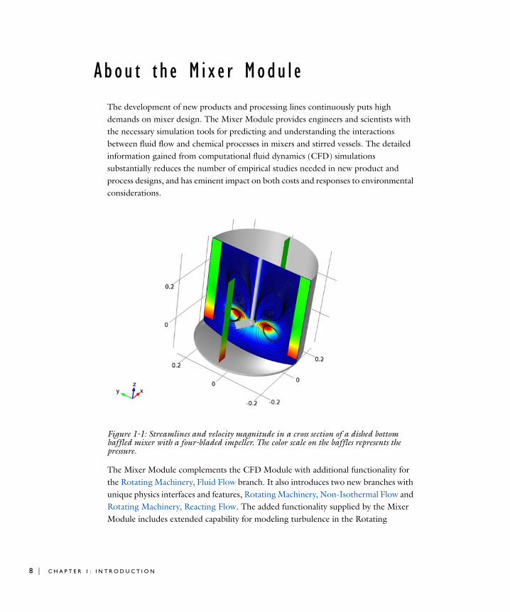
The development of new products and processing lines continuously puts high demands on mixer design. The Mixer Module provides engineers and scientists with the necessary simulation tools for predicting and understanding the interactions between fluid flow and chemical processes in mixers and stirred vessels. The detailed information gained from computational fluid dynamics (CFD) simulations substantially reduces the number of empirical studies needed in new product and process designs, and has eminent impact on both costs and responses to environmental considerations.

Figure 1-1: Streamlines and velocity magnitude in a cross section of a dished bottom baffled mixer with a four-bladed impeller. The color scale on the baffles represents the pressure.

The Mixer Module complements the CFD Module with additional functionality for the Rotating Machinery, Fluid Flow branch. It also introduces two new branches with unique physics interfaces and features, Rotating Machinery, Non-Isothermal Flow and Rotating Machinery, Reacting Flow. The added functionality supplied by the Mixer Module includes extended capability for modeling turbulence in the Rotating

1 : I N T R O D U C T I O N

Machinery interfaces. A high rotation rate or a strong acceleration of the rotation rate may induce a substantial deformation of the free surface in an open vessel. This topology change in turn influences the flow pattern inside the vessel. The Mixer Module includes free-surface features to capture the displacement of the liquid-air interface induced by the bulk motion in the domain, by the walls, and by the rotating shaft.

The physics interfaces define a fluid-flow problem using physical quantities such as pressure, flow rate, temperature, and species composition, as well as physical properties, such as viscosity, thermal diffusivity, and density. The different physics interfaces cover a wide range of laminar and turbulent mixer flows. The conservation laws formulated by the physics interfaces are expressed in terms of partial differential equations along with corresponding initial and boundary conditions. The equations are solved by the module using stabilized finite element formulations for fluid flow in combination with damped Newton methods and, for time-dependent problems, in combination with various time-dependent solver algorithms. The Mixer Module’s general capabilities include frozen-rotor and time-dependent flows in two- and three-dimensional spaces. For a so-called frozen-rotor flow, the topology relative to the rotating reference frame is fixed (“frozen”). When the flow field is, or can be approximated to be, of this type the computational time (CPU time) can be substantially reduced using the Frozen Rotor (see the CFD Module User’s Guide) study type.

The workflow in the Mixer Module is quite straightforward. Set up a simulation using one of the Rotating Machinery interfaces, described by the following steps: define the geometry, select the fluid to be modeled, select the type of flow, define boundary and initial conditions, define the finite element mesh, select a solver, and visualize the results. All these steps are performed from the COMSOL Desktop. The mesh and solver steps are usually carried out automatically using default settings, which are tuned specifically for each fluid-flow interface.

The models available in the Mixer Module model library describe the physics interfaces and their features through examples for different types of mixer flows. Here you find models of industrial equipment and devices, tutorial models for practice, and benchmark models for verification and validation of the fluid-flow interfaces. Go to The Model Libraries Window to access these resources.

To help you get started, this introduction contains a list of the physics interfaces and an example, Tutorial Example—Non-Isothermal Mixer, to introduce you to the workflow.

A B O U T T H E M I X E R M O D U L E | 9

10 | C H A P T E R

A S P E C T S O F M I X E R S I M U L A T I O N S

In the initial stages of development for a product or new process line, the focus usually lies on qualitative results such as determining whether or not the flow is well mixed, whether a heated reactor is free from hot-spots, or whether the flow field contains recirculation zones, which can be inaccessible to reactants. Qualitative results such as these are usually the first step toward creating or improving a design. During the later stages of development, the focus shifts toward scale-up and optimization. For mixing of pseudoplastic slurries the yield stress has to be overcome everywhere. Bioreactors, for example, should not contain regions of excessive shear. Obtaining accurate estimates for the yield stress, shear or other process parameters such as reaction rates, thermal equilibration times, torque, and energy consumption, provides developers with the edge needed to assume a competitive position within their field.

The choice of which physics to include in your simulations can be based on experimental results, experience, or a dimensional analysis. Excluding relevant physics undoubtedly leads to wrong results, while including “everything” leads to excessive computational time. The Rotating Machinery interfaces help you set up problems of varying complexity. If the mixed quantity is passive, you can use one of the Rotating Machinery, Fluid Flow interfaces to solve for the fluid flow, and then add a Transport of Diluted Species interface to determine other properties, for example, the mixing efficiency. Both reactions and thermal variations affect constitutive quantities, such as the density and viscosity of the fluid. When these effects become appreciable, you can switch to the Rotating Flow, Reacting Flow interfaces or the Rotating Flow, Non-Isothermal Flow interfaces. Taking it one step further, COMSOL Multiphysics lets you add other physics interfaces to preexisting ones to tailor simulations to your application.

The physics interfaces in the Mixer Module are able to perform all steps in mixer analyses, from the initial idea and qualitative simulations to the final optimization of the product and/or process.

The Mixer Module Interfaces

The Rotating Machinery interfaces in this module are based on the laws for conservation of momentum, mass, energy, and species composition in fluids. The different physics interfaces contain different combinations and expressions of the conservation laws, which apply to the physics of the flow field being modeled.


Figure 1-2 shows the Rotating Machinery interfaces as they are displayed when you add a physics interface (see The Physics Interface List by Space Dimension and Study Type). A short description of the physics interfaces follows.

Figure 1-2: The Rotating Machinery interfaces for laminar and turbulent flow.

R O T A T I N G M A C H I N E R Y, F L U I D F L O W

The Rotating Machinery, Laminar Flow interface ( ) is used primarily for modeling flows of low to intermediate Reynolds numbers. This physics interface solves the Navier-Stokes equations for incompressible and weakly compressible flow (up to Mach 0.3). The physics interface is also capable of simulating non-Newtonian fluid flow.

The Rotating Machinery, Turbulent Flow interfaces ( ) are used to model flow at high Reynolds numbers. These physics interfaces solve the Reynolds-averaged Navier-Stokes (RANS) equations for the averaged velocity field and averaged pressure. The different physics interfaces in this branch have different models for the turbulent viscosity. There are several turbulence models available—a standard k- model, a k-


12 | C H A P T E R

model, and a low Reynolds number k- model. Similarly to the Rotating Machinery,

Laminar Flow interface, compressibility (Mach < 0.3) is selected by default.

The standard k- model is the most widely used turbulence model because it is often a good compromise between accuracy and computational cost (memory and CPU time). The k- model is an alternative to the standard k- model and often gives more accurate results, especially in recirculation regions and close to solid walls. However, the k- model is also less robust than the standard k- model. The low Reynolds number k- model is more accurate than the standard k- model, especially close to walls, but it requires higher resolution in the near-wall region.

R O T A T I N G M A C H I N E R Y , N O N - I S O T H E R M A L F L O W

The Rotating Machinery, Non-Isothermal Flow, Laminar Flow interface ( ) is used primarily to model laminar rotating flow where the temperature and flow fields have to be coupled, such as in an externally heated mixer. This physics interface has predefined functionality for coupling heat transfer in fluids and solids.

The Rotating Machinery, Non-Isothermal Flow, Turbulent Flow interfaces ( ) solve the Reynolds-averaged Navier-Stokes (RANS) equations together with the equations for heat transfer in fluids and in solids. Besides the standard k- model, there is support for additional RANS turbulence models—a k- model and a low Reynolds number k- model.

R O T A T I N G M A C H I N E R Y , R E A C T I N G F L O W

The Rotating Machinery, Reacting Flow interfaces ( ) combine the functionality of the Rotating Machinery, Fluid Flow and Transport of Concentrated Species interfaces. The mass and momentum transport in a rotating reacting fluid can be modeled from a single physics interface, and the couplings between the velocity field and mixture density are set up automatically. Physics interfaces for both laminar flow and turbulent flow using the Reynolds-averaged Navier-Stokes (RANS) equations are available. The supported RANS models include the standard k- model, a k- model, and a low Reynolds number k- model.


T H E P H Y S I C S I N T E R F A C E L I S T B Y S P A C E D I M E N S I O N A N D S T U D Y TY P E

INTERFACE ICON TAG SPACE DIMENSION

AVAILABLE PRESET STUDY TYPE

Chemical Species Transport

Rotating Machinery, Reacting Flow

Laminar Flow rmrf 3D, 2D, frozen rotor; time dependent;

Turbulent Flow

Turbulent Flow, k- rmrf 3D, 2D frozen rotor; time dependent

Turbulent Flow, k- rmrf 3D, 2D frozen rotor; time dependent

Turbulent Flow, Low Re k- rmrf 3D, 2D frozen rotor with initialization; transient with initialization

Fluid Flow

Single-Phase Flow

Rotating Machinery, Fluid Flow

Rotating Machinery, Laminar Flow

rmspf 3D, 2D frozen rotor; time dependent

Rotating Machinery, Turbulent Flow, k-


Rotating Machinery, Turbulent Flow, k-


Rotating Machinery, Turbulent Flow, Low Re k-

rmspf 3D, 2D frozen rotor with initialization; transient with initialization


14 | C H A P T E R

Where Do I Access the Documentation?

A number of Internet resources provide more information about COMSOL, including licensing and technical information. The electronic documentation, topic-based (or context-based) help, and the Model Libraries are all accessed through the COMSOL Desktop.

T H E D O C U M E N T A T I O N A N D O N L I N E H E L P

The COMSOL Multiphysics Reference Manual describes all core physics interfaces and functionality included with the COMSOL Multiphysics license. This book also has instructions about how to use COMSOL and how to access the electronic Documentation and Help content.

Non-Isothermal Flow

Rotating Machinery, Non-Isothermal Flow

Laminar Flow rmnitf 3D, 2D frozen rotor; time dependent

Turbulent Flow, k- rmnitf 3D, 2D frozen rotor; time dependent

Turbulent Flow, k- rmnitf 3D, 2D frozen rotor; time dependent

Turbulent Flow, Low Re k- rmnitf 3D, 2D frozen rotor with initialization; transient with initialization

INTERFACE ICON TAG SPACE DIMENSION

AVAILABLE PRESET STUDY TYPE

If you are reading the documentation as a PDF file on your computer, the blue links do not work to open a model or content referenced in a different guide. However, if you are using the Help system in COMSOL Multiphysics, these links work to other modules (as long as you have a license), model examples, and documentation sets.


Opening Topic-Based HelpThe Help window is useful as it is connected to many of the features on the GUI. To learn more about a node in the Model Builder, or a window on the Desktop, click to highlight a node or window, then press F1 to open the Help window, which then displays information about that feature (or click a node in the Model Builder followed by the Help button ( ). This is called topic-based (or context) help.

Opening the Documentation Window

To open the Help window:

• In the Model Builder, click a node or window and then press F1.

• On any toolbar (for example, Home or Geometry), hover the mouse over a button (for example, Browse Materials or Build All) and then press F1.

• From the File menu, click Help ( ).

• In the upper-right part of the COMSOL Desktop, click the ( ) button.

To open the Help window:

• In the Model Builder, click a node or window and then press F1.

• On the main toolbar, click the Help ( ) button.

• From the main menu, select Help>Help.

To open the Documentation window:

• Press Ctrl+F1.

• From the File menu select Help>Documentation ( ).

To open the Documentation window:

• Press Ctrl+F1.

• On the main toolbar, click the Documentation ( ) button.

• From the main menu, select Help>Documentation.


16 | C H A P T E R

T H E M O D E L L I B R A R I E S W I N D O W

Each model includes documentation that has the theoretical background and step-by-step instructions to create the model. The models are available in COMSOL as MPH-files that you can open for further investigation. You can use the step-by-step instructions and the actual models as a template for your own modeling and applications. In most models, SI units are used to describe the relevant properties, parameters, and dimensions in most examples, but other unit systems are available.

Once the Model Libraries window is opened, you can search by model name or browse under a module folder name. Click to highlight any model of interest and a summary of the model and its properties is displayed, including options to open the model or a PDF document.

Opening the Model Libraries WindowTo open the Model Libraries window ( ):

C O N T A C T I N G C O M S O L B Y E M A I L

For general product information, contact COMSOL at [email protected].

To receive technical support from COMSOL for the COMSOL products, please contact your local COMSOL representative or send your questions to

The Model Libraries Window in the COMSOL Multiphysics Reference Manual.

• From the Home ribbon, click ( ) Model Libraries.

• From the File menu select Model Libraries.

To include the latest versions of model examples, from the File>Help menu, select ( ) Update COMSOL Model Library.

• On the main toolbar, click the Model Libraries button.

• From the main menu, select Windows>Model Libraries.

To include the latest versions of model examples, from the Help menu select ( ) Update COMSOL Model Library.


[email protected]. An automatic notification and case number is sent to you by email.

C O M S O L WE B S I T E S

COMSOL website www.comsol.com

Contact COMSOL www.comsol.com/contact

Support Center www.comsol.com/support

Product Download www.comsol.com/support/download

Product Updates www.comsol.com/support/updates

COMSOL Community www.comsol.com/community

Events www.comsol.com/events

COMSOL Video Gallery www.comsol.com/video

Support Knowledge Base www.comsol.com/support/knowledgebase


http://www.comsol.com

http://www.comsol.com/contact/

http://www.comsol.com/support/

http://www.comsol.com/support/download/

http://www.comsol.com/support/updates

http://www.comsol.com/community

http://www.comsol.com/events/

http://www.comsol.com/video/

http://www.comsol.com/support/knowledgebase/

18 | C H A P T E R

Ove r v i ew o f t h e U s e r ’ s Gu i d e

The Mixer Module User’s Guide gets you started with modeling using COMSOL Multiphysics and provides information specific to this module. Further instructions on using COMSOL in general are found in the COMSOL Multiphysics Reference Manual.

For general information about setting up and solving CFD models, see the CFD Module User’s Guide.

The last section in this chapter features a model you can access from the The Model Libraries Window. The Tutorial Example—Non-Isothermal Mixer solves a mixer-flow problem using the Laminar Flow interface in the Rotating Machinery, Non-Isothermal

Flow branch.

The next chapter introduces you to the Theory for the Free Surface Features. It includes descriptions of the mesh deformation within the free surface domain and the conditions that need to be satisfied at a free surface, at a three-phase boundary, and on a rotating shaft.

The remaining three chapters describe the new physics interfaces and features under the Rotating Machinery, Fluid Flow branch, and the two additional branches that are exclusive to the Mixer Module: Rotating Machinery, Non-Isothermal Flow and Rotating Machinery, Reacting Flow.

As detailed in the section Where Do I Access the Documentation? this information can also be found from the COMSOL Multiphysics software Help menu.


Tu t o r i a l E x amp l e—Non - I s o t h e rma l M i x e r

This model demonstrates how to obtain the temperature distribution in a simplified tabletop lab mixer using the Rotating Machinery, Non-Isothermal Flow branch in the Mixer Module. The key instructive element is a demonstration of the Frozen Rotor

method, which substantially reduces the computational time for a mixing study.

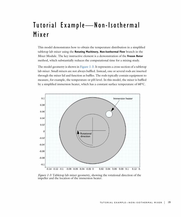
The model geometry is shown in Figure 1-3. It represents a cross-section of a tabletop lab mixer. Small mixers are not always baffled. Instead, one or several rods are inserted through the mixer lid and function as baffles. The rods typically contain equipment to measure, for example, the temperature or pH level. In this model, the mixer is baffled by a simplified immersion heater, which has a constant surface temperature of 60°C.

Figure 1-3: Tabletop lab mixer geometry, showing the rotational direction of the impeller and the location of the immersion heater.

Immersion heater

Rotationaldirection

TU T O R I A L E X A M P L E — N O N - I S O T H E R M A L M I X E R | 19

20 | C H A P T E R

The mixer tank is filled with water that is agitated by the impeller, which rotates clockwise (as indicated in Figure 1-3) with 20 rotations per minute (rpm). The impeller blades are modeled as infinitely thin.

The tank is made of steel and is subjected to cooling by natural convection that takes place on the outside of the mixer. The surrounding conditions are temperature equal to 20 °C and pressure equal to 1 atmosphere, and the reactor is 0.2 m high. These conditions are needed as input for the natural convection correlations, which are used to calculate the heat transfer coefficient from the tank wall to the surroundings.

M O D E L S E T U P

The Reynolds number for a mixer is commonly calculated as

(1-1)

where N is the number of rotations per second, Da the impeller diameter, and the kinematic viscosity. A high Reynolds number means that the flow has a tendency to become turbulent. Evaluating Equation 1-1 using at 60 °C gives Re = 6944. This Reynolds number would warrant the use of a turbulence model, if the model were three-dimensional. But the restriction to two dimensions makes the flow remain laminar at higher Reynolds numbers and a turbulence model is therefore not applied. A possible extension of the model is to apply a turbulence model and recalculate the result to investigate the effect of possible turbulent structures in the flow.

The objective of this model is to obtain the temperature distribution at operating conditions. One way to get there would be to start from zero velocity and a homogeneous temperature distribution and to simulate the start-up of the mixer. This approach is simple, but requires a relatively long computation time.

A computationally more efficient method is to first simulate the flow using the frozen-rotor approach. The frozen-rotor approach is a modeling concept that treats the rotor as fixed, or frozen in space. The flow in the rotating domain is assumed to be stationary in terms of a rotating coordinate system. The effect of the rotation is then accounted for by the Coriolis and centrifugal forces. The flow in the non-rotating parts is also assumed to be stationary, but in a non-rotating coordinate system. (See Frozen Rotor in the CFD Module User’s Guide for more information.) The result of a frozen-rotor simulation is an approximation to the flow induced by the impeller. The result depends on the angular position of the impeller and cannot represent transient effects. However, it is still a very good starting point to reach operating conditions.

ReNDa

2

-------------=


The frozen-rotor result is used as input to a time-dependent simulation and the progress towards the operating conditions is monitored using probe plots.

R E S U L T S A N D D I S C U S S I O N

Figure 1-4 shows the velocity distribution obtained from the frozen-rotor simulation. As expected, the highest velocity magnitude is found at the tip of the mixer blades. There are three recirculation zones: one downstream of the immersion heater, one along the top wall, and one along the bottom wall.

Figure 1-4: Velocity field obtained from the frozen rotor simulation.

Figure 1-5 shows the temperature distribution obtained from the frozen-rotor simulation. Streamlines are also included to visualize the flow field. The temperature is relatively homogeneous throughout the mixer. There are some cold spots in connection to the recirculation zones adjacent to the outer wall. This is expected since the fluid there has a longer residence time close to the solid wall, and therefore has less contact with the heated fluid closer to the center of the mixer.


22 | C H A P T E R

Figure 1-5: Temperature distribution obtained from the frozen-rotor simulation.

The progress of a solution can be monitored using probes (see Probes in the COMSOL Multiphysics Reference Manual). The velocity magnitude and temperature are probed at xy0.050.065. The location is indicated in Figure 1-5, just outside the recirculation zone along the top wall.

The probe plots produced during the time-dependent simulation are shown in Figure 1-6. Both plots show that the flow pattern and temperature distribution begin to shift away from the frozen-rotor solution and correspond more closely to the operating conditions. The shift in the velocity value is significant, but the temperature does not shift much.

The velocity probe plot clearly shows the frequency that corresponds to the passing of the blades. It also contains a frequency that corresponds to two full revolutions of the impeller (one full revolution of the impeller takes 3 seconds). The temperature value does not display those rapid variations but changes smoothly.

Probe point


Figure 1-6: Probe plots of velocity and temperature in the mixer from the time-dependent simulation.


24 | C H A P T E R

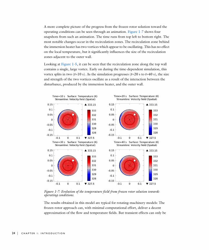
A more complete picture of the progress from the frozen-rotor solution toward the operating conditions can be seen through an animation. Figure 1-7 shows four snapshots from such an animation. The time runs from top left to bottom right. The most notable changes occur in the recirculation zones. The recirculation zone behind the immersion heater has two vortices which appear to be oscillating. This has no effect on the local temperature, but it significantly influences the size of the recirculation zones adjacent to the outer wall.

Looking at Figure 1-5, it can be seen that the recirculation zone along the top wall contains a single, large vortex. Early on during the time-dependent simulation, this vortex splits in two (t10 s). As the simulation progresses (t20 s to t40 s), the size and strength of the two vortices oscillate as a result of the interaction between the disturbance, produced by the immersion heater, and the outer wall.

Figure 1-7: Evolution of the temperature field from frozen rotor solution towards operating conditions.

The results obtained in this model are typical for rotating-machinery models: The frozen-rotor approach can, with minimal computational effort, deliver a decent approximation of the flow and temperature fields. But transient effects can only be


captured with a time-dependent simulation, and these effects can change local temperature and velocity values significantly.

The remainder of this section consists of step-by-step instructions on setting up, solving, and analyzing the model using both solver types.

M O D E L W I Z A R D

The first step to build a model is to open COMSOL, then select the physics interface and specify the type of analysis you want to do—in this case, a frozen-rotor Rotating Machinery, Non-Isothermal Laminar Flow analysis.

1 Open COMSOL Multiphysics. On the New page, click Model Wizard . Then click the 2D button .

2 In the Select physics tree, select Fluid Flow>Non-Isothermal Flow>Rotating Machinery,

Non-Isothermal Flow>Laminar Flow (rmnitf) .

3 Click the Add button.

4 Click the Study button .

5 In the tree, select Preset Studies>Frozen Rotor .

6 Click the Done button .

C R E AT E T H E G E O M E T R Y

To simplify this step, insert a prepared geometry sequence. Go to the Geometry desktop toolbar.

1 On the Geometry toolbar, choose Insert Sequence .

2 Browse to the Module’s models folder and double-click the file nonisothermal_mixer.mph.

3 Go to the Home toolbar and choose Build All . The Home toolbar refers to the specific set of controls near the top of the Desktop.

4 Click the Zoom Extents button on the Graphics toolbar.

M A T E R I A L S

On the Home toolbar, click Add Material .


26 | C H A P T E R

Water, liquid1 Go to the Add Material window.

2 In the tree, select Built-In>Water, liquid.

3 In the Add Material window, click Add to Component .

Steel AISI 43401 Go to the Add Material window.

2 In the tree, select Built-In>Steel AISI 4340.

3 In the Add Material window, click Add to Component .

4 In the Model Builder window, under Component 1>Materials click Steel AISI 4340.

5 Select Domain 1, the circular outer rim of the mixer, only.

6 On the Home toolbar, click Add Material again to close the Add Material window.

R O T A T I N G M A C H I N E R Y , N O N - I S O T H E R M A L F L O W

Go to the Physics toolbar.

Heat Transfer in Solids 11 On the Physics toolbar, click Domains and choose Heat Transfer in Solids .


2 Select Domain 1 only.

Rotating Domain 11 On the Physics toolbar, click Domains and choose Rotating Domain .

2 Select Domain 3, the impeller, only.

3 In the Rotating Domain settings window, locate the Rotating Domain section.

4 In the Revolutions per time edit field, type 20[1/min].

Rotating Interior Wall 11 On the Physics toolbar, click Boundaries and choose Rotating Interior Wall .

2 Select Boundaries 17–20, the impeller blades.

Heat Continuity 11 On the Physics toolbar, click Pairs and choose Heat Continuity .

2 In the Heat Continuity settings window, locate the Pair Selection section.

3 In the Pairs list, select Identity Pair 1.

Flow Continuity 21 On the Physics toolbar, click Pairs and choose Flow Continuity .

2 In the Flow Continuity settings window, locate the Pair Selection section.

3 In the Pairs list, select Identity Pair 1.

Convective Heat Flux 11 On the Physics toolbar, click Boundaries and choose Convective Heat Flux .

2 Select Boundaries 1, 2, 7, and 12, which make up the circular outer boundary of the mixer.


28 | C H A P T E R

3 In the Convective Heat Flux settings window, locate the Heat Flux section.

4 From the Heat transfer coefficient list, choose External natural convection.

5 In the L edit field, type 0.2[m].

Temperature 11 On the Physics toolbar, click Boundaries and choose Temperature .

2 Select Boundaries 13–16, which make up the boundary of the immersion heater.

3 In the Temperature settings window, locate the Temperature section.

4 In the T0 edit field, type 60[degC].

Pressure Point Constraint 11 On the Physics toolbar, click Points and choose Pressure Point Constraint .

2 Select Point 5 only. This is the bottommost point on the outer boundary of the mixer.

M E S H 1

1 In the Model Builder window, under Component 1 click Mesh 1 .

2 In the Mesh settings window, from the Element size list, choose Fine.

The default mesh only generates one cell across the solid domain. Use a boundary layer mesh in the solid to increase the resolution there.

3 Go to the Mesh toolbar and click Edit .

4 In the Model Builder window, under Component 1>Mesh 1 click Boundary

Layers 1 .

5 Select Domains 1–3 only.


6 Go to the Home toolbar.

S T U D Y 1

1 On the Home toolbar, click Compute .

R E S U L T S

Re-create Figure 1-4 using the following steps.

Velocity (rmnitf)1 Got to the Velocity (rmnitf) toolbar and choose Streamline .

2 In the Streamline settings window, locate the Streamline Positioning section.

3 From the Positioning list, choose Uniform density.

4 In the Separating distance edit field, type 0.02.

5 Locate the Coloring and Style section. From the Color list, choose White.

6 On the Velocity (rmnitf) toolbar, click Plot .

7 Click the Zoom Extents button on the Graphics toolbar.

Figure 1-5 can be created by the following steps.

Temperature (rmnitf)1 In the Model Builder window, expand the Results>Temperature (rmnitf) node, then

click Surface 1 .

2 In the Surface settings window, locate the Coloring and Style section.

3 From the Color table list, choose Wave.

4 Go to the Temperature (rmnitf) toolbar and choose Streamline .





30 | C H A P T E R

8 Locate the Coloring and Style section. From the Color list, choose Gray.

9 On the Temperature (rmnitf) toolbar, click Plot .

Add a probe to follow the development of the flow during the time-dependent simulation.

D E F I N I T I O N S

1 Go to the Definitions toolbar, click Probes and choose Domain Point Probe .

2 In the Domain Point Probe settings window, locate the Point Selection section.

3 In the Coordinates edit field, set x to -0.05[m].

4 In the Coordinates edit field, set y to 0.065[m].

The probe is located at the outer edge of the recirculation zone that is positioned along the upper wall.

5 In the Model Builder window, expand the Component 1>Definitions>Domain Point

Probe 1 node .

6 Right-click Point Probe Expression 1 and choose Duplicate.

7 In the Point Probe Expression settings window, locate the Expression section.

8 In the Expression edit field, type T.

9 Click to expand the Table and Window

Settings section. From the Plot window list, choose New window.

Add a Time Dependent study.

R O O T

On the Home toolbar, click Add Study .


M O D E L W I Z A R D

1 Go to the Add Study window.

2 In the tree, select Preset Studies>Time Dependent .

3 In the Add Study window, click Add Study .

S T U D Y 2

Step 1: Time Dependent1 In the Model Builder window, under Study 2, click Step 1: Time Dependent .

2 In the Time Dependent settings window, locate the Study Settings section.

3 In the Times edit field, type range(0,0.5,40).

4 Click to expand the Values of Dependent Variables section. Select the Initial values of

variables solved for check box.

5 From the Method list, choose Solution.

6 From the Study list, choose Study 1, Frozen Rotor.

7 On the Home toolbar, click Compute .

Two probe plots automatically display when you start the calculation.

R E S U L T S

Probe 1D Plot Group 8The following steps create an animation that contains the plots in Figure 1-7.


32 | C H A P T E R

Temperature (rmnitf) 1Plot the data set edges on the spatial frame to make them follow the rotation.

1 In the Model Builder window under Results , click Temperature (rmnitf) 1 .

2 In the 2D Plot Group settings window, locate the Plot Settings section.

3 From the Frame list, choose Spatial (x, y, z).

4 In the Model Builder window, expand the Temperature (rmnitf) 1 node, then click Surface 1 .

5 In the Surface settings window, locate the Coloring and Style section.

6 From the Color table list, choose Wave.

7 Go to the Temperature (rmnitf) 1 toolbar and choose Streamline .




11 Locate the Coloring and Style section. From the Color list, choose Gray.

Export1 Go to the Results toolbar and click Player .

2 In the Player settings window, locate the Scene section.

3 From the Subject list, choose Temperature (rmnitf) 1.

4 Locate the Frames section. From the Frame selection list, choose All.

5 Locate the Playing section. In the Display each frame for edit field, type 0.25.

6 On the Graphics toolbar, click Play .


2

M i x e r M o d u l e T h e o r y

In this chapter:

• Theory for the Free Surface Features

33

34 | C H A P T E R

Th eo r y f o r t h e F r e e S u r f a c e F e a t u r e s

In this section:

• Free Surface Domain

• Free Surface Conditions

• Contact Angle

• Rotating Shaft Conditions

• References for the Free Surface Features

Free Surface Domain

The mesh within the free surface domain is deformed to account for the movement of the free surface. This mesh movement is accomplished using a moving mesh approach. The software perturbs the mesh nodes so that they conform with the free surface and with other moving or stationary boundaries in the model. The boundary displacement is propagated throughout the domain to obtain a smooth mesh deformation everywhere. This is done by solving a Laplace smoothing equation for the mesh displacement. Taking two dimensions as an example, a location in the deformed mesh with coordinates (x, y) can be related to its coordinates in the original undeformed mesh (X,Y) by a function on the form:

The original, undeformed, mesh is referred to as the material frame (or reference frame), while the deformed mesh is called the spatial frame. COMSOL Multiphysics also defines geometry and mesh frames, which are coincident with the material frame for this physics interface.

Theory for the Rotating Machinery Interfaces and Theory for the Non-Isothermal Flow and Conjugate Heat Transfer Interfaces in the CFD Module User’s Guide

The links to the physics features described in other guides do not work in the PDF, only from the online help in COMSOL Multiphysics.

x x X Y t y y X Y t = =

2 : M I X E R M O D U L E T H E O R Y

For the Rotating Machinery interfaces the fluid-flow equations (along with other coupled equations such as heat or chemical species transport) are solved in the spatial frame in which the mesh is perturbed.

Free Surface Conditions

The Free Surface feature assumes that the density and viscosity of the fluid outside the domain are negligible compared to the corresponding values inside the domain. On the free surface the following condition for the viscous stress, , along the surface is applied:

(2-1)

Here pext is the pressure outside the free surface domain (SI unit: Pa) and fst denotes the surface tension forces (SI unit: N/m2). In the surface tension terms, s is the surface gradient operator (sIni ni

Twhere I is the identity matrix and is the surface tension coefficient (SI unit: N/m).

The mesh velocity at the free surface is defined as the fluid velocity in the direction normal to the surface:

(2-2)

Contact Angle

At a three-phase boundary, it is necessary to add force terms to ensure that the fluid maintains a consistent contact angle. The forces acting at the contact point are applied to the fluid by the Contact Angle node (added per default under a Free Surface node). In equilibrium, the surface tension forces and the normal restoring force from the surface are in balance at a contact angle (c), as shown in Figure 2-1. This equilibrium is expressed by Young's equation, which considers the components of the forces in the plane of the surface:

(2-3)

Deformed Geometry and Moving Mesh in the COMSOL Multiphysics Reference Manual

ni pextn– i fst+ pextn– i + s ni ni s–= =

umesh n u n =

c cos s1+ s2=

T H E O R Y F O R T H E F R E E S U R F A C E F E A T U R E S | 35

36 | C H A P T E R

where is the surface tension between the two fluids, s1 is the surface energy density on the wetted side, and s2 the surface energy density on the other side of the two-phase interface.

Figure 2-1: The forces acting at a contact point. In equilibrium, the surface tension forces and the normal restoring force from the surface are in balance at a contact angle c.

There is still debate in the literature as to precisely what occurs in nonequilibrium situations (for example, drop impact) when the physical contact angle deviates from the contact angle specified by Young’s equation. A simple approach, is to assume that the unbalanced part of the in-plane Young force acts on the fluid to move the contact angle toward its equilibrium value (Ref. 1). COMSOL Multiphysics employs this approach as it is physically motivated and is consistent with the from thermodynamics allowed form of the boundary condition (Ref. 2, Ref. 3).

The normal force balance at the solid surface is handled by the wall boundary condition, which automatically prevents fluid flow across the solid boundary through a no-penetration condition. The wall fluid interface feature applies a force, fwf, on the fluid at the interface:

where is the actual contact angle and ms is the binormal to the solid surface.

Rotating Shaft Conditions

Using a Rotating Shaft feature, the velocity of the shaft boundary is defined by assuming solid body rotation of the shaft. The wall velocity is hence a function of the angular velocity w (SI unit: rad/s) of the shaft, and the (spatial frame) position x:

(2-4)

fwf c cos cos– ms=

uw wraxrax------- x rbp– =


where rax and rbp is the rotation axis direction and rotation base point, respectively.

References for the Free Surface Features

1. J. Gerbeau and T. Lelievre, “Generalized Navier Boundary Condition and Geometric Conservation Law for Surface Tension,” Computer Methods In Applied Mechanics and Engineering, vol. 198, pp. 644–656, 2009.

2. W. Ren and E. Weinan, “Boundary Conditions for the Moving Contact Line Problem,” Physics of Fluids, vol. 19, p. 022101, 2007.

3. W. Ren and D. Hu, “Continuum Models for the Contact Line Problem,” Physics of Fluids, vol. 22, p. 102103, 2010.

T H E O R Y F O R T H E F R E E S U R F A C E F E A T U R E S | 37

38 | C H A P T E R

3

R o t a t i n g M a c h i n e r y , F l u i d F l o w

The Rotating Machinery, Laminar Flow (rmspf) and Rotating Machinery, Turbulent Flow

(rmspf) interfaces, found under the Single-Phase Flow>Rotating Machinery

branch ( ) when adding a physics interface, are used for modeling flow where one or more of the boundaries rotate in a periodic fashion. This is used for mixers and propellers.

The physics interfaces support compressible and incompressible flow, the flow of non-Newtonian fluids described by the Power Law and Carreau models, and also turbulent flow. The physics interfaces also support creeping flow, although the shallow channel approximation is redundant.

In this chapter:

• The Rotating Machinery, Laminar Flow Interface

• The Rotating Machinery, Turbulent Flow, k- Interface

• The Rotating Machinery, Turbulent Flow, k- Interface

• The Rotating Machinery, Turbulent Flow, Low Re k- Interface

• Domain, Boundary, Point, and Pair Nodes for the Rotating Machinery, Laminar and Turbulent Flow Interfaces

39

40 | C H A P T E R

Th e Ro t a t i n g Ma ch i n e r y , F l u i d F l ow I n t e r f a c e s

The Rotating Machinery, Laminar Flow Interface

The Rotating Machinery, Laminar Flow (rmspf) interface ( ), found under the Single-Phase Flow>Rotating Machinery branch ( ) when adding a physics interface, is used to simulate flow at low to moderate Reynolds numbers in geometries with one or more rotating parts. The physics interface supports incompressible and compressible flows at low Mach numbers (typically less than 0.3). It also supports modeling of non-Newtonian fluids. The physics interface is available for 3D and 2D models.

There are two study types available for this physics interface. Using the Time Dependent study type, rotation is achieved through moving mesh functionality, also known as sliding mesh. Using the Frozen Rotor study type, the rotating parts are kept frozen in position, and rotation is accounted for by the inclusion of centrifugal and Coriolis forces. In both types, the momentum balance is governed by the Navier-Stokes equations, and the mass conservation is governed by the continuity equation. See Theory for the Rotating Machinery Interfaces in the CFD Module User’s Guide.

When this physics interface is added, the following default physics nodes are also added in the Model Builder—Fluid Properties, Wall, Rotating Wall, and Initial Values. Then, from the Physics toolbar, add other nodes that implement, for example, boundary conditions and volume forces. You can also right-click Rotating Machinery, Laminar Flow

to select physics from the context menu. See Rotating Domain, Initial Values, and Rotating Wall.

I N T E R F A C E I D E N T I F I E R

The interface identifier is used primarily as a scope prefix for variables defined by the physics interface. Refer to these variables in expressions using the pattern <identifier>.<variable_name>. In order to distinguish between variables belonging to different physics interfaces, the identifier string must be unique. Only letters, numbers and underscores (_) are permitted in the Identifier field. The first character must be a letter.

3 : R O T A T I N G M A C H I N E R Y , F L U I D F L O W

The default identifier (for the first physics interface in the component) is rmspf.

A D V A N C E D S E T T I N G S

To display this section, click the Show button ( ) and select Advanced Physics Options. Normally these settings do not need to be changed.

Pseudo time steppingSelect the Use pseudo time stepping for stationary equation form check box to add pseudo time derivatives to the equation when the Frozen Rotor equation form is used. (Frozen rotor is a pseudo stationary formulation.) When selected, also choose a CFL

number expression—Automatic (the default) or Manual. Automatic sets the local CFL number (from the Courant–Friedrichs–Lewy condition) to the built-in variable CFLCMP which in turn triggers a PID regulator for the CFL number. If Manual is selected, enter a Local CFL number CFLloc (dimensionless).

Mesh Smoothing TypeThis setting controls the method used to solve for the mesh displacement inside free surface domains. The Mesh smoothing type can be chosen to be Laplace (the default), Winslow, Hyperelastic, or Yeoh smoothing. Note that the equations used for each smoothing type have different properties. The default, Laplace smoothing, usually is the most robust choice.

In addition to the settings described below, see The Laminar Flow, Creeping Flow, and Turbulent Flow Interfaces in the CFD Module User’s Guide for all the other settings available.

Also go to Domain, Boundary, Point, and Pair Nodes for the Rotating Machinery, Laminar and Turbulent Flow Interfaces for links to all the physics nodes.

• Pseudo Time Stepping for Laminar Flow Models in the CFD Module User’s Guide

• Pseudo Time Stepping in the COMSOL Multiphysics Reference Manual

This physics interface changes to the Rotating Machinery, Turbulent Flow, k-interface when the Turbulence model type selected is Rans, k-.

T H E R O T A T I N G M A C H I N E R Y , F L U I D F L O W I N T E R F A C E S | 41

42 | C H A P T E R

The Rotating Machinery, Turbulent Flow, k- Interface

The Rotating Machinery, Turbulent Flow, k- (rmspf) interface ( ), found under the Single-Phase Flow>Rotating Machinery branch ( ) when adding a physics interface, is used to simulate flow at high Reynolds numbers in geometries with one or more rotating parts. The physics interface is suitable for incompressible and compressible flows at low Mach numbers (typically less than 0.3).

The momentum balance is governed by the Navier-Stokes equations, and the mass conservation is governed by the continuity equation. Turbulence effects are modeled using the standard two-equation k- model with realizability constraints. Flow close to walls is modeled using wall functions.

There are two study types available for this physics interface. Using the Time Dependent study type, the rotation is achieved through moving mesh functionality, also known as sliding mesh. Using the Frozen Rotor study type, the rotating parts are kept frozen in position, and the rotation is accounted for by the inclusion of centrifugal and Coriolis forces. See Theory for the Rotating Machinery Interfaces in the CFD Module User’s Guide.

When this physics interface is added, the following physics nodes are also added in the Model Builder—Fluid Properties, Wall, Rotating Wall, and Initial Values. Then, from the Physics toolbar, add other nodes that implement, for example, boundary conditions and volume forces. You can also right-click Rotating Machinery, Turbulent Flow, k- to select physics from the context menu. See Rotating Domain, Initial Values, and Rotating Wall in this section for details.

Laminar Flow in a Baffled Stirred Mixer: model library path CFD_Module/

Single-Phase_Tutorials/baffled_mixer

See The Laminar Flow, Creeping Flow, and Turbulent Flow Interfaces in the CFD Module User’s Guide for all the settings. Also go to Domain, Boundary, Point, and Pair Nodes for the Rotating Machinery, Laminar and Turbulent Flow Interfaces for links to all the physics nodes.


The Rotating Machinery, Turbulent Flow, k- Interface

The Rotating Machinery, Turbulent Flow, k- (rmspf) interface ( ), found under the Single-Phase Flow>Rotating Machinery branch ( ) when adding a physics interface, is used to simulate flow at high Reynolds numbers in geometries with one or more rotating parts. The physics interface supports incompressible and compressible flows at low Mach numbers (typically less than 0.3). The physics interface is available for 3D and 2D models.

The momentum balance is governed by the Navier-Stokes equations, and the mass conservation is governed by the continuity equation. Turbulence effects are modeled using Wilcox revised two-equation k- model with realizability constraints. Flow close to walls is modeled using wall functions.

There are two study types available for this physics interface. Using the Time Dependent study type, the rotation is achieved through moving mesh functionality, also known as sliding mesh. Using the Frozen Rotor study type, the rotating parts are kept frozen in position, and the rotation is accounted for by the inclusion of centrifugal and Coriolis forces. See Theory for the Rotating Machinery Interfaces in the CFD Module User’s Guide.

When this physics interface is added, the following default physics nodes are also added in the Model Builder—Fluid Properties, Wall, Rotating Wall, and Initial Values. Then, from the Physics toolbar, add other nodes that implement, for example, boundary conditions and volume forces. You can also right-click Rotating Machinery, Turbulent

Flow, k-to select physics from the context menu. See Rotating Domain, Initial Values, and Rotating Wall in this section for details.

This physics interface changes to Rotating Machinery, Laminar Flow when the Turbulence model type selected is None.

See The Laminar Flow, Creeping Flow, and Turbulent Flow Interfaces in the CFD Module User’s Guide for all other settings. Also go to Domain, Boundary, Point, and Pair Nodes for the Rotating Machinery, Laminar and Turbulent Flow Interfaces for links to all the physics nodes.


44 | C H A P T E R

The Rotating Machinery, Turbulent Flow, Low Re k- Interface

The Rotating Machinery, Turbulent Flow, Low Re k- (rmspf) interface ( ), found under the Single-Phase Flow>Rotating Machinery branch ( ) when adding a physics interface, is used to simulate flow at high Reynolds numbers in geometries with one or more rotating parts. The physics interface supports incompressible and compressible flows at low Mach numbers (typically less than 0.3). The physics interface is available for 3D and 2D models.

The momentum balance is governed by the Navier-Stokes equations, and the mass conservation is governed by the continuity equation. Turbulence effects are modeled using the AKN two-equation k- model with realizability constraints. The AKN model is a so-called low-Reynolds number model, which means that it resolves the flow all the way down to the wall. The AKN model depends on the distance to the closest wall. The physics interface therefore includes a wall distance equation.

There are two study types available for this physics interface. Using the Transient with

Initialization study type, the rotation is achieved through moving mesh functionality, also known as sliding mesh. Using the Frozen Rotor with Initialization study type, the rotating parts are kept frozen in position, and the rotation is accounted for by the inclusion of centrifugal and Coriolis forces. See Theory for the Rotating Machinery Interfaces in the CFD Module User’s Guide.

When this physics interface is added, the following default physics nodes are also added in the Model Builder—Fluid Properties, Wall, Rotating Wall, and Initial Values.Then, from the Physics toolbar, add other nodes that implement, for example, boundary conditions and volume forces. You can also right-click Rotating Machinery, Turbulent

Flow, Low Re k-to select physics from the context menu. See Rotating Domain, Initial Values, and Rotating Wall in this section for details.


See The Laminar Flow, Creeping Flow, and Turbulent Flow Interfaces in the CFD Module User’s Guide for all other settings. Also go to Domain, Boundary, Point, and Pair Nodes for the Rotating Machinery, Laminar and Turbulent Flow Interfaces for links to all the physics nodes.


Domain, Boundary, Point, and Pair Nodes for the Rotating Machinery, Laminar and Turbulent Flow Interfaces

The Rotating Machinery, Laminar Flow Interface and The Rotating Machinery, Turbulent Flow, k- Interface have the following domain, boundary, point, and pair physics nodes, which are available from the Physics ribbon toolbar (Windows users), Physics context menu (Mac or Linux users), or right-click to access the context menu (all users).

The following nodes (listed in alphabetical order) are described for the Laminar Flow interface in the CFD Module User’s Guide:


In general, to add a node, go to the Physics toolbar, no matter what operating system you are using.

• Initial Values

• Rotating Domain

• Rotating Wall

• Rotating Interior Wall


• Free Surface

• Contact Angle

• Navier Slip

• Rotating Shaft

• No Viscous Stress

• Flow Continuity

• Fluid Properties

• Inlet

• Interior Wall

• Line Mass Source

• Open Boundary

• Outlet

• Periodic Flow Condition

• Point Mass Source

• Pressure Point Constraint

• Screen

• Symmetry

• Volume Force

• Wall


46 | C H A P T E R

Initial Values

The Initial Values node adds initial values for the velocity field and pressure that can serve as initial conditions for a transient simulation or as an initial guess for a nonlinear solver.

D O M A I N S E L E C T I O N

For a default node, the setting inherits the selection from the parent node, and can not be edited; that is, the selection is automatically made and is the same as for the physics interface. When nodes are added from the context menu, you can select Manual from the Selection list to choose specific domains or select All domains as required.

I N I T I A L V A L U E S

Enter values or expressions for the initial value of the Velocity field u (SI unit: ms) (the default is 0 ms) and for the Pressure p (SI unit: Pa) (the default value is 0 Pa).

For The Rotating Machinery, Turbulent Flow, k- Interface also enter values for the Turbulent kinetic energy (SI unit: m2s2) and Turbulent dissipation rate (SI unit: m2s3).

Rotating Domain

Use the Rotating Domain node to specify the rotational frequency and direction in the Rotating Machinery, Fluid Flow interfaces.

The angular displacement, (SI unit: rad), of the rotating domain is computed from a specified angular velocity w (SI unit: rads) by solving the ODE

(3-1)

Since the angular displacement is solved for, the domain rotation can be specified using any type of angular velocity (constant, analytic, interpolation function, and so forth).

If there is more than one rotating domain, these must not intersect.

ddt-------- w t =


R O T A T I N G D O M A I N

Rotating Wall

The Rotating Wall node is a boundary condition for The Rotating Machinery, Laminar Flow Interface and The Rotating Machinery, Turbulent Flow, k- Interface. The feature applies to external boundaries of a Rotating Domain. It applies flow conditions corresponding to no slip (laminar flow) or wall functions (for turbulent flow) as defined by the Wall node described in the CFD Module User’s Guide, but accounts for the velocity of the Rotating Domain.

For 3D models, select the Axis of rotation, the z-axis is the default. If the x-axis is selected, it corresponds to a rotational axis (1, 0, 0) with the origin as the base point. This is the same for the y-axis and z-axis. If User

defined is selected, enter values for the Rotation axis base point rbp (SI unit: m) and Rotation axis direction rax.

Select a Rotational frequency—Revolutions per time (the default) or Angular

velocity.

• If Revolutions per time is selected, enter a value or expression in the field (SI unit: 1s) and select a Rotational direction—Positive angular velocity

(the default) or Negative angular velocity. The angular velocity in this case is defined as the input multiplied by 2·.

• If Angular velocity is selected, enter an Angular velocity w (SI unit: rads). The default is 0 rads.

For 2D models, enter coordinates for the Rotation axis base point rbp (SI unit: m). The default is the origin (0, 0).

Select a Rotational frequency—Revolutions per time (the default) or Angular

velocity.

• If Revolutions per time is selected, enter a value or expression in the field (SI unit: 1s) and select a Rotational direction—Clockwise (the default) or Counterclockwise. The angular velocity in this case is defined as the input multiplied by 2·.

• If Angular velocity is selected, enter an Angular velocity w (SI unit: rads). The default is 0 rads.


48 | C H A P T E R

B O U N D A R Y S E L E C T I O N

For a default node, the setting inherits the selection from the parent node, and can not be edited; that is, the selection is automatically made and is the same as for the physics interface. When nodes are added from the context menu, you can select Manual from the Selection list to choose specific boundaries or select All boundaries as required.

C O N S T R A I N T S E T T I N G S

To display this section, click the Show button ( ) and select Advanced Physics Options. Select the Use weak constraints check box to use weak constraints and create dependent variables for the corresponding Lagrange multipliers.

Rotating Interior Wall

The Rotating Interior Wall node is a boundary condition for The Rotating Machinery, Laminar Flow Interface and The Rotating Machinery, Turbulent Flow, k- Interface. The feature applies Rotating Wall conditions to internal boundaries of a Rotating Domain.

The feature is similar to the Rotating Wall boundary condition, available on exterior boundaries, except that it applies on both sides of an internal boundary. It allows discontinuities (velocity, pressure, turbulence) across the boundary. You can use the Rotating Interior Wall boundary condition to avoid meshing thin structures by instead applying conditions on interior curves and surfaces.


For a default node, the setting inherits the selection from the parent node, and can not be edited; that is, the selection is automatically made and is the same as for the physics interface. When nodes are added from the context menu, you can select Manual from the Selection list to choose specific fluid boundaries subjected to a rotating interior wall, or select All boundaries as required.

References for the Single-Phase Flow, Turbulent Flow Interfaces

References for the Single-Phase Flow, Turbulent Flow Interfaces


Free Surface Domain

Use the Free Surface Domain node to specify domains which are bounded by a free surface. Inside free surface domains, the mesh position is solved for while accounting for the position of the free surface. On external boundaries not defined as a free surface, the mesh is constrained to move only in the tangential direction. On boundaries which are internal with respect to the fluid, the mesh elements are kept at their initial position.


From the Selection list, choose the domains on which to apply the condition.

Free Surface

The Free Surface node is used to define the free surface separating an interior modeled fluid from the outer fluid. The free surface follows the fluid motion, in the normal direction, and is governed by the fluid motion in the free surface domain and the surface tension of the fluid-fluid interface.

To control the attachment angle between the free surface and adjacent walls, a Contact Angle node is by default added under the Free Surface node.


From the Selection list, choose the boundaries on which to apply the condition.

F R E E S U R F A C E

Enter an External pressure pext (SI unit: Pa) corresponding to the pressure level in the external fluid phase.

If there is more than one free surface domain, these must not intersect. Also a free surface domain cannot intersect with a rotating domain.

The Free Surface node can only be applied to outer boundaries of a Free Surface Domain.


50 | C H A P T E R

S U R F A C E TE N S I O N

The default Surface tension coefficient (SI unit: Nm) is User defined. It can also be specified from predefined libraries, by selecting Library coefficient, liquid/gas interface or Library coefficient, liquid/liquid interface.

• If Library coefficient, liquid/gas interface is selected, select an option from the list—Water/Air, Acetone/Air, Acetic acid/Air, Ethanol/Air, Ethylene glycol/Ethylene glycol

vapor, Diethyl ether/Air, Glycerol/Air, Heptane/Nitrogen, Mercury/Mercury vapor, or Toluene/Air.

• If Library coefficient, liquid/liquid interface is selected, select an option from the list—Benzene/Water, 20°C, Corn oil/Water, 20°C, Ether/Water, 20°C, Hexane/Water, 20°C, Mercury/Water, 20°C, or Olive oil/Water, 20°C.

Contact Angle

The Contact Angle node specifies the contact angle between the free surface and the solid wall. The node applies forces on the wall that balance the surface tension for the prescribed contact angle.

The representation of the contact angle is dependent on the mesh resolution in the region where the fluid-fluid interface attaches to the wall. If, during the simulation, the contact angle is found to fluctuate around a given value, this indicates that the resolution needs to be improved. This can for example be achieved by adding more mesh boundary layers on the wall.

E D G E O R PO I N T S E L E C T I O N

From the Selection list, choose the geometric entity (edges or points) that represent the three phase contact.

C O N T A C T A N G L E

Select an option from the Specify contact angle list—Directly (the default) or Through

Young’s equation.

• If Directly is selected, enter a Contact angle w (SI unit: rad). The default is 2.

For laminar flow the Contact Angle node is only available on edges or points where a Navier Slip boundary condition is applied adjacent to the free surface. In this case the Navier Slip condition is required for the contact line to move along the wall.


If Through Young’s equation is selected, enter values or expressions for Phase 1-Solid

surface energy density s1 (SI unit: Jm2) and Phase 2-Solid surface energy density s2 (SI unit: Jm2).

Navier Slip

The Navier Slip boundary condition is suitable for walls adjacent to a free surface when solving for laminar flow. Applying this boundary condition, the contact line (fluid-fluid-solid interface) is free to move along the wall.

The boundary condition enforces no-penetration at the wall, u·nwall = 0 and adds a frictional force of the form

where is a slip length. The slip length is defined as = hmin2, where hmin is the smallest element side among the elements along the wall. The boundary condition does not set the tangential velocity component to zero; however, the extrapolated tangential velocity component is 0 at a distance outside of the wall.

It is recommended that Navier Slip is applied only on the walls that the free surface contact line passes.



Rotating Shaft

Use the Rotating Shaft node to define boundaries where the fluid is subjected to a solid shaft rotation. This feature should be applied to boundaries outside of, but connecting to, a rotating domain.



Ffr---u–=

The Navier Slip feature is disabled when selecting a turbulence model. For turbulent flow, a Wall feature using wall functions is required for the contact line to be free to move along the wall.


52 | C H A P T E R

R O T A T I N G S H A F T

Axis of RotationSelect the Axis of rotation. If x-axis is selected, this corresponds to a rotational axis (1, 0, 0) with the origin as the base point. Correspondingly, if y-axis or z-axis is selected, the rotational axis is defined by a unit vector in the selected direction together with a base point at the origin. If User defined is selected, enter values into these fields: Rotation axis base point and Rotation axis direction. The z-axis is the default choice and the default values in the fields for User defined correspond to those for the z-axis.

Angular VelocitySelect the rotating shaft Angular velocity from the list:

• Select the User defined option to manually define the angular velocity (SI unit: rads). This is the default setting.

• Select an angular velocity defined by a present Rotating Domain feature, to which the shaft is connected, for example Angular velocity rmspf/rd1.


4

R o t a t i n g M a c h i n e r y , N o n - I s o t h e r m a l F l o w

In this chapter:

• Rotating Machinery, Non-Isothermal Flow, Laminar Flow Interface

• Rotating Machinery, Non-Isothermal Flow, Turbulent Flow, k- Interface


• Rotating Machinery, Non-Isothermal Flow, Turbulent Flow, Low Re k-Interface

• For links to all the nodes, go to Domain, Boundary, Edge, Point, and Pair Nodes for the Rotating Machinery, Non-Isothermal Flow, Laminar and Turbulent Flow Interfaces

53

54 | C H A P T E R

Th e Ro t a t i n g Ma ch i n e r y , Non - I s o t h e rma l F l ow I n t e r f a c e s

Rotating Machinery, Non-Isothermal Flow, Laminar Flow Interface

The Laminar Flow version of the Rotating Machinery, Non-Isothermal Flow (rmnitf)

interface ( ), found under the Fluid Flow>Non-Isothermal Flow>Rotating Machinery,

Non-Isothermal Flow branch when adding a physics interface, is used to simulate laminar flow and heat transfer in equipment containing one or more rotating parts.

The physics interface can be used to simulate fluid flows where the fluid properties depend on the temperature. Models can also include heat transfer in solids, stationary and rotating, as well as surface-to-surface radiation and radiation in participating media. Conservation of energy, mass, and momentum is solved for in fluids, while in solids conservation of energy is solved for. The physics interface supports low Mach number (typically less than 0.3) flows. It also supports non-Newtonian fluids.

There are two study types available for this physics interface. Using the Time Dependent study type, the rotation is achieved through moving mesh functionality, also known as sliding mesh. Using the Frozen Rotor study, the rotating parts are kept frozen in position, and the rotation is accounted for by the inclusion of centrifugal and Coriolis forces.

This physics interface combines the Rotating Machinery, Laminar Flow interface with the Non-Isothermal Flow interface. Adding the physics interface, the following default nodes are also added in the Model Builder—Fluid, Thermal Insulation, Wall, Rotating Wall,

and Initial Values. This physics interface is available in 2D and 3D.



The default identifier (for the first physics interface in the component) is rmnitf.

4 : R O T A T I N G M A C H I N E R Y , N O N - I S O T H E R M A L F L O W


The default setting is to have All domains in the component define the fluid pressure, temperature and velocity and the equations that describe these fields. To choose specific domains, select Manual from the Selection list.

P H Y S I C A L M O D E L

The default Turbulence model type is None. Select the Neglect inertial term (Stokes flow) check box to model flow at very low Reynolds numbers for which the inertial term in the Navier-Stokes equations can be neglected. The physics interface then solves the linear Stokes equations. This flow type is referred to as creeping flow or Stokes flow and can occur in microfluidics applications (and MEMS devices), where the flow length scales are very small.

D E P E N D E N T V A R I A B L E S

The dependent variables (field variables) for this physics interface are:

• the Velocity field u and its components (SI unit: ms). The default is 0 ms.

• the Pressure p (SI unit: Pa). The default is 0 Pa.

• the Temperature T (SI unit: K). The default is 293.15 K (20 degrees Celsius, or room temperature).

If required, edit the field, component, and dependent variable names. Editing the name of a scalar dependent variable changes both its field name and the dependent variable name. If a new field name coincides with the name of another field of the same type, the fields share degrees of freedom and dependent variable names. A new field name must not coincide with the name of a field of another type, or with a component name belonging to some other field. Component names must be unique within a model except when two fields share a common field name.

D I S C R E T I Z A T I O N

To display this section, click the Show button ( ) and select Discretization. It controls the discretization (the element types used in the finite element formulation). From the Discretization of fluids list select the element order for the velocity components and the pressure: P1+P1 (the default), P2+P1, or P3+P2.

• P1+P1 (the default) uses linear elements for both the velocity components and the pressure field. This is the default element order for the Laminar Flow and Turbulent

Flow interfaces. Linear elements are computationally cheaper than higher-order elements and are also less prone to introduce spurious oscillations, thereby improving the numerical robustness.

T H E R O T A T I N G M A C H I N E R Y , N O N - I S O T H E R M A L F L O W I N T E R F A C E S | 55

56 | C H A P T E R

• P2+P1 uses second-order elements for the velocity components and linear elements for the pressure field. This is the default for the Creeping Flow interface because second-order elements work well for low flow velocities.

• P3+P2 uses third-order elements for the velocity components and second-order elements for the pressure field. This can add additional accuracy but it also adds additional degrees of freedom compared to P2+P1 elements.

The discretization of the temperature field follows that of the fluid components. So the temperature order is 1 for P1+P1, 2 for P2+P1, and 3 for P3+P2.

Select a Surface radiosity—Linear (the default), Quadratic, Cubic, Quartic, or Quintic (2D axisymmetric and 2D models only).

Specify the Value type when using splitting of complex variables—Real (the default) or Complex for each of the Dependent variables in the table.

C O N S I S T E N T S T A B I L I Z A T I O N

To display this section, click the Show button ( ) and select Stabilization. The consistent stabilization methods are applicable to the Heat and flow equations. By default, both the check boxes are selected. Streamline diffusion provides optimal performance for heat transfer in fluids or other applications that include a convective or translational term. Crosswind diffusion provides extra diffusion in regions with sharp gradients. The added diffusion is orthogonal to the streamlines, so streamline diffusion and crosswind diffusion can be used simultaneously.

I N C O N S I S T E N T S T A B I L I Z A T I O N

To display this section, click the Show button ( ) and select Stabilization. The Isotropic diffusion inconsistent stabilization method can be activated for both the Heat

equation and the Navier-Stokes equations. Enter a Tuning parameter id. The default for both the Heat equation and Navier-Stokes equations is 0.25.



The Use pseudo time stepping for stationary equation form check box is selected by default to add pseudo time derivatives to the equation when the Stationary equation form is used. When selected, also choose a CFL number expression—Automatic (the default) or Manual. Automatic calculates the local CFL number (from the Courant-Friedrichs-Lewy condition) from a built-in expression. If Manual is selected, enter a Local CFL number CFLloc.


By default the Enable conversions between material and spatial frames check box is selected.

Rotating Machinery, Non-Isothermal Flow, Turbulent Flow, k- Interface

The Turbulent Flow, k-version of the Rotating Machinery, Non-Isothermal Flow (rmnitf) interface ( ), found under the Fluid Flow>Non-Isothermal Flow>Rotating Machinery,

Non-Isothermal Flow branch when adding a physics interface, is used to simulate turbulent flow and heat transfer in equipment containing one or more rotating parts.

The physics interface can be used to model fluid flow and energy transport in single-phase flows at high Reynolds numbers. Models can also include heat transfer in solids, stationary and rotating, as well as surface-to-surface radiation and radiation in participating media. The physics interface supports low Mach number (typically less than 0.3) flows.

The physics interface solves for conservation of energy, mass, and momentum in fluids, and for conservation of energy in solids. Turbulence effects are modeled using the standard two-equation k-model with realizability constraints. Flow and heat transfer close to walls are modeled using wall functions.

There are two study types available for this physics interface. Using the Time Dependent study type, the rotation is achieved through moving mesh functionality, also known as sliding mesh. Using the Frozen Rotor study, the rotating parts are kept frozen in

• Domain, Boundary, Edge, Point, and Pair Nodes for the Rotating Machinery, Non-Isothermal Flow, Laminar and Turbulent Flow Interfaces

• Theory for the Free Surface Features

In the CFD Module User’s Guide:

• Pseudo Time Stepping for Laminar Flow Models

• The Projection Method for the Navier-Stokes Equations

In the COMSOL Multiphysics Reference Manual:

• About Frames in Heat Transfer

• Pseudo Time Stepping


58 | C H A P T E R

position, and the rotation is accounted for by the inclusion of centrifugal and Coriolis forces.

This physics interface combines the Rotating Machinery, Turbulent Flow, k-interface and the Non-Isothermal Flow interface.


The default Turbulence model type is RANS and the default Turbulence model is k- for this physics interface.

The default Heat transport turbulence model is Kays-Crawford. Other options are Extended Kays-Crawford or User-defined turbulent Prandtl number.

• The Extended Kays-Crawford model requires a Reynolds number at infinity. That input is given in the Model Inputs section of the Fluid feature node.

• It is always possible to specify a user-defined model for the turbulent Prandtl number. Enter the user-defined value or expression for the Turbulent Prandtl number in the Model Inputs section of the Fluid feature node.

TU R B U L E N C E M O D E L P A R A M E T E R S

Turbulence model parameters are optimized to fit as many flow types as possible, but for some special cases, better performance can be obtained by tuning the model parameters. For a description of the turbulence model and the included model parameters see Theory for the Turbulent Flow Interfaces in the CFD Module User’s Guide.



• the Velocity field u and its components (SI unit: ms). The default is 0 ms.

• the Pressure p (SI unit: Pa). The default is 0 Pa.


• the Turbulent kinetic energy k (SI unit: m2s2)

• the Turbulent dissipation rate ep (SI unit: m2s3)

Except for the settings described below, see Rotating Machinery, Non-Isothermal Flow, Laminar Flow Interface for details.


If required, edit the field, component, and dependent variable names. Editing the name of a scalar dependent variable changes both its field name and the dependent variable name. If a new field name coincides with the name of another field of the same type, the fields share degrees of freedom and dependent variable names. A new field name must not coincide with the name of a field of another type, or with a component name belonging to some other field. Component names must be unique within a model except when two fields share a common field name.

C O N S I S T E N T A N D I N C O N S I S T E N T S T A B I L I Z A T I O N

To display these sections, click the Show button ( ) and select Stabilization. In addition to the equations described for the Rotating Machinery, Non-Isothermal Flow, Laminar Flow Interface, the consistent and inconsistent stabilization methods are also applicable to the Turbulence equations.


To display this section, click the Show button ( ) and select Advanced Physics Options. Normally these settings do not need to be changed. In addition to the parameters described for the Rotating Machinery, Non-Isothermal Flow, Laminar Flow Interface, the Turbulence variables scale parameters subsection contains the parameters Uscale and Lfact that are used to calculate absolute tolerances for the turbulence variables.

The scaling parameters must only contain numerical values, units, or parameters defined under Global Definitions. The scaling parameters can not contain variables. The parameters are used when a new default solver for a transient study step is generated. If you change the parameters, the new values take effect the next time a new default solver is generated.

Rotating Machinery, Non-Isothermal Flow, Turbulent Flow, k- Interface

The Turbulent Flow, k-version of the Rotating Machinery, Non-Isothermal Flow (rmnitf) interface ( ), found under the Fluid Flow>Non-Isothermal Flow>Rotating Machinery,

• Rotating Machinery, Non-Isothermal Flow, Laminar Flow Interface




60 | C H A P T E R

Non-Isothermal Flow branch when adding a physics interface, is used to simulate turbulent flow and heat transfer in equipment containing one or more rotating parts.


The physics interface solves for conservation of energy, mass, and momentum in fluids and for conservation of energy in solids. Turbulence effects are modeled using the Wilcox revised two-equation k- model with realizability constraints. Flow and heat transfer close to walls are modeled using wall functions.

There are two study types available for this physics interface. Using the Time Dependent study type, the rotation is achieved through moving mesh functionality, also known as sliding mesh. Using the Frozen Rotor study type, the rotating parts are kept frozen in position, and the rotation is accounted for by the inclusion of centrifugal and Coriolis forces.

This physics interface combines the Rotating Machinery, Turbulent Flow, k-interface and the Non-Isothermal Flow interface.





• the Velocity field u and its components (SI unit: ms)

• the Pressure p (SI unit: Pa)


Except for the settings described below, see Rotating Machinery, Non-Isothermal Flow, Laminar Flow Interface and Rotating Machinery, Non-Isothermal Flow, Turbulent Flow, k- Interface.



• the Specific dissipation rate om (SI unit: 1s)

Rotating Machinery, Non-Isothermal Flow, Turbulent Flow, Low Re k-Interface

The Turbulent Flow, Low Re k-version of the Rotating Machinery, Non-Isothermal Flow

(rmnitf) interface ( ), found under the Fluid Flow>Non-Isothermal Flow>Rotating

Machinery, Non-Isothermal Flow branch when adding a physics interface, is used to simulate turbulent flow and heat transfer in equipment containing one or more rotating parts.


The physics interface solves for conservation of energy, mass, and momentum in fluids and for conservation of energy in solids. Turbulence effects are modeled using the AKN two-equation k- model with realizability constraints. The AKN model is a so-called low-Reynolds number model, which means that it resolves the flow and heat transfer all the way down to the wall. The AKN model depends on the distance to the closest wall. The physics interface therefore includes a wall distance equation.

There are two study types available for this physics interface. Using the Transient with

Initialization study type, the rotation is achieved through moving mesh functionality, also known as sliding mesh. Using the Frozen Rotor with Initialization study type, the rotating parts are kept frozen in position, and the rotation is accounted for by the inclusion of centrifugal and Coriolis forces.




62 | C H A P T E R

This physics interface combines the Rotating Machinery, Turbulent Flow, Low Re k-interface and the Non-Isothermal Flow interface.


The default Turbulence model type is RANS and the default Turbulence model is Low

Reynolds number k- for this physics interface.


The dependent variables (field variables) for this interface are:





• the Turbulent dissipation rate ep (SI unit: m2/s3)

• the Reciprocal wall distance G (SI unit: 1m)

Domain, Boundary, Edge, Point, and Pair Nodes for the Rotating Machinery, Non-Isothermal Flow, Laminar and Turbulent Flow Interfaces

Except for the settings described below, see Rotating Machinery, Non-Isothermal Flow, Laminar Flow Interface and Rotating Machinery, Non-Isothermal Flow, Turbulent Flow, k- Interface.



The links to the nodes described in the CFD Module User’s Guide guides do not work in the PDF, only from the on line help in COMSOL Multiphysics.


All versions of the Rotating Machinery, Non-Isothermal Flow interfaces have the following domain, boundary, edge, point, and pair nodes available from the Physics ribbon toolbar (Windows users), Physics context menu (Mac or Linux users), or right-click to access the context menu (all users).

Except for Initial Values, described here, the following nodes are described for the Rotating Machinery, Fluid Flow interfaces: The Free Surface, Navier Slip, and Rotating

Shaft nodes are selected from the Free Surface Conditions submenu:


• Free Surface

• Contact Angle

• Navier Slip

• Rotating Shaft (3D Only)

The following nodes are described for the Non-Isothermal Flow interfaces in the CFD Module User’s Guide:

The following nodes are described for the single-phase flow Rotating Machinery,

Laminar Flow interface in the CFD Module User’s Guide:

• Rotating Domain


• Rotating Wall (this is selected from the Rotating Machinery, Laminar Flow menu)

In general, to add a node, go to the Physics toolbar, no matter what operating system you are using. However, to add subnodes, right-click the parent node.

• Fluid

• Interior Wall

• Open Boundary

• Pressure Work

• Symmetry, Flow

• Symmetry, Heat and Symmetry, Flow

• Viscous Heating

• Wall


64 | C H A P T E R

The following nodes are described for the Single-Phase Flow, Laminar Flow interface in the CFD Module User’s Guide: Some of the nodes are selected from the Rotating

Machinery, Laminar Flow submenu.

The following nodes are described for the Heat Transfer interface in the CFD Module User’s Guide. Some of the nodes are selected from the Heat Transfer submenu.

Initial Values

The Initial Values node adds initial values for the dependent variables that can serve as initial conditions for a transient simulation or as an initial guess for a nonlinear solver.


• Flow Continuity

• Inlet

• Outlet



• Volume Force

• Vacuum Pump

• Wall (for the pair node)

• Boundary Heat Source

• Continuity

• Convective Heat Flux

• Heat Flux

• Heat Source

• Heat Transfer in Solids

• Inflow Heat Flux

• Line Heat Source

• Outflow

• Periodic Heat Condition

• Point Heat Source

• Pressure Work

• Surface-to-Ambient Radiation

• Temperature

• Thermal Insulation

• Thin Thermally Resistive Layer

In the COMSOL Multiphysics Reference Manual:

• Periodic Condition and Destination Selection

• Periodic Boundary Conditions



For a default node, the setting inherits the selection from the parent node, and can not be edited; that is, the selection is automatically made and is the same as for the interface. When nodes are added from the context menu, you can select Manual from the Selection list to choose specific domains or select All domains as required.


Enter values or expressions for the initial value of the Velocity field u (SI unit: m/s), the Pressure p (SI unit: Pa), and the Temperature T (SI unit: K). The default values are 0 for the velocity field and pressure, and 293.15 K for the temperature.

For turbulence models, default initial values for the turbulence variables (as defined in Theory for the Turbulent Flow Interfaces in the CFD Module User’s Guide), are applied.


66 | C H A P T E R

5

R o t a t i n g M a c h i n e r y , R e a c t i n g F l o w

In this chapter:

• The Rotating Machinery, Reacting Flow, Laminar Flow Interface

• The Rotating Machinery, Reacting Flow, Turbulent Flow, k- Interface


• The Rotating Machinery, Reacting Flow, Turbulent Flow, Low Re k-Interface

• For links to all the nodes, go to Domain, Boundary, Point, and Pair Nodes for the Rotating Machinery, Reacting Flow, Laminar Flow and Turbulent Flow Interface

67

68 | C H A P T E R

Th e Ro t a t i n g Ma ch i n e r y , R e a c t i n g F l ow I n t e r f a c e s

The Rotating Machinery, Reacting Flow, Laminar Flow Interface

The Laminar Flow version of the Rotating Machinery, Reacting Flow (rmrf) interface ( ) is used to simulate the laminar flow and transport of chemical species in equipment containing one or more rotating parts. Reactions between the participating species can also be studied.

This physics interface solves for the instantaneous velocity and pressure fields, together with an arbitrary number of mass fractions. The momentum balance is governed by the Navier-Stokes equations, and the total mass conservation is governed by the continuity equation. For the chemical species, the governing transport equations include convection, diffusion and, optionally, migration in an electric field.

There are two study types available for this physics interface. For the Time Dependent study type the rotation is achieved by moving mesh functionality, also known as sliding mesh. For the Frozen Rotor study type (see Frozen Rotor in the CFD Module User’s Guide), the rotating parts are kept frozen in position, and the rotation is accounted for by the inclusion of centrifugal and Coriolis forces.

The physics interface combines the functionality of the Rotating Machinery, Laminar

Flow and the Reacting Flow interfaces.

The Rotating Machinery, Reacting Flow (rmrf) interface is added to the Model Builder after selecting any option under the Chemical Species

Transport>Rotating Machinery, Reacting Flow> branch when adding a physics interface.


• Theory for the Rotating Machinery Interfaces

• Theory for the Reacting Flow Interfaces

• Theory for the Transport of Concentrated Species Interface

5 : R O T A T I N G M A C H I N E R Y , R E A C T I N G F L O W

When this physics interface is added, the following default nodes are also added in the Model Builder—Fluid, No Flux, Wall, Rotating Wall, and Initial Values. Then, from the Physics toolbar, add other nodes that implement, for example, boundary conditions. You can also right-click the node to select physics from the context menu.



The default identifier (for the first physics interface in the component) is rmrf.


The default setting is to have All domains in the component define the dependent variables and the equations. To choose specific domains, select Manual from the Selection list.

S P E C I E S

Select the type of fluid mixture to study.

• Select Dilute solution (the default) when studying low concentration solutes present in a solvent with significantly higher concentration. Then, from the Solvent list, choose the species not solved for.

• Select Concentrated species when studying a mixture of species with comparable concentrations. Then, from the From mass constraint list, select the species not solved for. Use the species with the highest concentration in order to minimize the impact of any numerical errors.

The mass fraction for one of the species can be calculated from the constraint that the sum of all mass fractions must be equal to one. There is then no need to solve a transport equation for this species.

In the case of an ideal gas, the fluid mixture type decides how the density is evaluated. It, however, does not effect the mass transport equations used. These solve for the species mass fractions for both mixture types.

T H E R O T A T I N G M A C H I N E R Y , R E A C T I N G F L O W I N T E R F A C E S | 69

70 | C H A P T E R


The default Turbulence model type is None. Select the Neglect inertial term (Stokes flow) check box to model flow at very low Reynolds numbers for which the inertial term in the Navier-Stokes equations can be neglected.

Under Mass transport mechanisms, select a Diffusion model—Mixture-averaged or Fick’s

law (the default). The choice in this section enables different options for the Fluid node.


Specify the Number of species. There must be at least two species. To add a single species, click the Add mass fraction button ( ) under the table. To remove a species, select it in the list and click the Remove mass fraction button ( ) under the table. Edit the names of the species mass fractions directly in the table.

In addition to the chemical species mass fractions (dimensionless), this physics interface defines the following dependent variables (fields):

• the Velocity field u and its components (SI unit: m/s)




• From the Regularization list, select On (the default) or Off. See the settings for The Transport of Concentrated Species Interface in the CFD Module User’s Guide for more information.

• The Use pseudo time stepping for stationary equation form check box is selected by default. Pseudo time derivatives are added when applying a Frozen Rotor study step. See Pseudo Time Stepping for Mass Transport in the CFD Module User’s Guide and the settings for The Laminar Flow Interface for more information.

• The CFL number expression is Automatic by default. Select Manual to enter a different value or expression for CFLloc (dimensionless).


D I S C R E T I Z A T I O N

To display this section, click the Show button ( ) and select Discretization. It controls the discretization (the element types used in the finite element formulation) and some related properties:

• Select an element order (shape function order) for the Mass fraction—Linear (the default), Quadratic, Cubic, or Quartic. See the settings for Transport of Concentrated

Species for more information.

• The Compute boundary fluxes check box is selected by default so that COMSOL Multiphysics computes predefined accurate boundary flux variables. The computations of the following boundary flux variables change so that:

- ndflux_c (where c is the dependent variable for the concentration) is the normal diffusive flux and corresponds to the accurate boundary flux when diffusion is the only contribution to the flux term. When transport in an electric field is included or when the conservative form of the equation is used, ndflux_c is instead computed directly from the dependent variable.

- ntflux_c (where c is the dependent variable for the concentration) is the normal total flux and corresponds to the accurate boundary flux plus additional transport terms, for example, the convective flux when you use the non-conservative form.

If you clear the Compute boundary fluxes check box, COMSOL Multiphysics instead computes the flux variables from the dependent variables using extrapolation.

• The Apply smoothing to boundary fluxes check box is selected by default. The smoothing can provide a more well-behaved flux value close to singularities.

• From the Discretization of fluids list select the element order for the velocity components and the pressure: P1+P1 (the default), P2+P1, or P3+P2 (where the first term is the order of the velocity field and the second term is the order of the pressure). See the settings for The Laminar Flow Interface for more information.

• Specify the Value type when using splitting of complex variables for each dependent variable in the table—Real (the default) or Complex.

C O N S I S T E N T A N D I N C O N S I S T E N T S T A B I L I Z A T I O N

To display these sections, click the Show button ( ) and select Stabilization.

There are two consistent stabilization methods available—Streamline diffusion and Crosswind diffusion. Both are active by default for the Fluid flow equations and Species

transport equations.


72 | C H A P T E R

The Residual setting applies to both of the consistent stabilization methods for the mass fractions. Approximate residual (the default) means that derivatives of the diffusion tensor components are neglected. This setting is usually accurate enough and computationally faster. If required, select Full residual.

For the Fluid flow equations and Species transport equations there is one inconsistent stabilization method, Isotropic diffusion, which is not active by default.

The Rotating Machinery, Reacting Flow, Turbulent Flow, k- Interface

The Turbulent Flow, k-version of the Rotating Machinery, Reacting Flow (rmrf) interface ( ), found under the Rotating Machinery, Reacting Flow>Turbulent Flow

branch when adding a physics interface, is used to simulate the turbulent flow and mixing of chemical species in equipment containing one or more rotating parts. Reactions between the participating species can also be studied.

This physics interface solves for the averaged velocity and pressure fields, together with an arbitrary number of averaged mass fractions. The momentum balance is governed by the averaged Navier-Stokes equations, and the total mass conservation is governed by the continuity equation. The fluid-flow turbulence is modeled using the standard two-equation k- model with realizability constraints. For the chemical species, the governing transport equations include convection, diffusion and, optionally, migration in an electric field. Flow close to solid walls is modeled using wall functions for the flow and species transport. Turbulent reactions are modeled using the eddy dissipation model.

There are two study types available for this interface. For the Time Dependent study type the rotation is achieved by moving mesh functionality, also known as sliding mesh. For the Frozen Rotor study type the rotating parts are kept frozen in position, and the rotation is accounted for by the inclusion of centrifugal and Coriolis forces.


• The Rotating Machinery, Laminar and Turbulent Flow Interfaces

• The Reacting Flow Interfaces

• The Transport of Concentrated Species Interface


This physics interface combines the functionality of the Rotating Machinery, Turbulent

Flow, k- and the Reacting Flow interfaces.



When a turbulence model is used, a model for the turbulent mass transport is also needed. Select a Mass transport turbulence model—Kays-Crawford (the default) or User

defined turbulent Schmidt number.




Turbulence model parameters are optimized to fit as many flow types as possible, but for some special cases, better performance can be obtained by tuning the model parameters.


Specify the Number of species. There must be at least two species. To add a single species, click the Add Mass Fraction button ( ) under the table. To remove a species, select it in the list and click the Remove Mass Fraction button ( ) under the table. Edit the names of the species mass fractions directly in the table.






Except for the settings described below, see The Rotating Machinery, Reacting Flow, Laminar Flow Interface.


74 | C H A P T E R

The Rotating Machinery, Reacting Flow, Turbulent Flow, k- Interface

The Turbulent Flow k-version of the Rotating Machinery, Reacting Flow (rmrf) interface ( ), found under the Rotating Machinery, Reacting Flow>Turbulent Flow


This physics interface solves for the averaged velocity and pressure fields, together with an arbitrary number of averaged mass fractions. The momentum balance is governed by the averaged Navier-Stokes equations, and the total mass conservation is governed by the continuity equation. The fluid-flow turbulence is modeled using the Wilcox revised k- model with realizability constraints. For the chemical species, the governing transport equations include convection, diffusion and, optionally, migration in an electric field. Flow close to solid walls is modeled using wall functions for the flow and species transport. Turbulent reactions are modeled using the eddy dissipation model.

There are two study types available for this interface. For the Time Dependent study type the rotation is achieved by moving mesh functionality, also known as sliding mesh. For the Frozen Rotor study type the rotating parts are kept frozen in position, and the rotation is accounted for by the inclusion of centrifugal and Coriolis forces.

The physics interface combines the functionality of the Rotating Machinery, Turbulent

Flow k- and the Reacting Flow interfaces.



When a turbulence model is used, a model for the turbulent mass transport is also needed. Select a Mass transport turbulence model—Kays-Crawford (the default) or User

defined turbulent Schmidt number.













• the Specific dissipation rate om (SI unit: 1s)

The Rotating Machinery, Reacting Flow, Turbulent Flow, Low Re k-Interface

The Turbulent Flow, Low Re k-version of the Rotating Machinery, Reacting Flow (rmrf) interface ( ), found under the Rotating Machinery, Reacting Flow>Turbulent Flow


This physics interface solves for the averaged velocity and pressure fields, together with an arbitrary number of averaged mass fractions. The momentum balance is governed by the averaged Navier-Stokes equations, and the total mass conservation is governed by the continuity equation. The fluid-flow turbulence is modeled using the AKN low-Reynolds number k- model. The low-Reynolds number model resolves the velocity, pressure and mass fractions all the way down to the wall. For this reason the interface is suited for studying mass transfer at high Schmidt numbers. The AKN


76 | C H A P T E R

model depends on the distance to the closest wall, and the physics interface therefore includes a wall distance equation. For the chemical species, the governing transport equations include convection, diffusion and, optionally, migration in an electric field. Turbulent reactions are modeled using the eddy dissipation model.

There are two study types available for this interface. For the Transient with

Initialization study type the rotation is achieved by moving mesh functionality, also known as sliding mesh. For the Frozen Rotor with Initialization study type the rotating parts are kept frozen in position, and the rotation is accounted for by the inclusion of centrifugal and Coriolis forces.

The physics interface combines the functionality of the Rotating Machinery, Turbulent

Flow, Low Re k- and the Reacting Flow interfaces.


The default Turbulence model type is RANS and the default Turbulence model is Low

Reynolds number k- for this physics interface.

When a turbulence model is used, a model for the turbulent mass transport is also needed. Select a Mass transport turbulence model—Kays-Crawford (the default), High

Schmidt number model, or User defined turbulent Schmidt number.










• the Velocity field u and its components (SI unit: m/s)




• the Reciprocal wall distance G (SI unit: 1/m)

Domain, Boundary, Point, and Pair Nodes for the Rotating Machinery, Reacting Flow, Laminar Flow and Turbulent Flow Interface

The Rotating Machinery, Reacting Flow Interfaces has these domain, boundary, point, and pair nodes available from the Physics ribbon toolbar (Windows users), Physics context menu (Mac or Linux users), or right-click to access the context menu (all users).

These nodes are described in this section:

• Fluid

• Initial Values

• Inflow

• Species Continuity

The following nodes are described for The Reacting Flow Interfaces in the CFD Module User’s Guide.

• Wall

• Reactions

• Reacting Boundary

• Open Boundary

In general, to add a node, go to the Physics toolbar, no matter what operating system you are using. However, to add subnodes, right-click the parent node.


78 | C H A P T E R

The following nodes are described for the Rotating Machinery, Fluid Flow interfaces. The Free Surface, Navier Slip, and Rotating Shaft nodes are selected from the Free Surface

Conditions submenu

The following nodes are described for The Laminar Flow Interface in the CFD Module User’s Guide (listed in alphabetical order). Some of the nodes are selected from the Fluid Flow submenu:

The following nodes (listed in alphabetical order) are described for The Transport of Concentrated Species Interface or The Transport of Diluted Species Interface in the CFD Module User’s Guide. Some of the nodes are selected from the Species Transport

submenu:


• Free Surface

• Contact Angle

• Navier Slip

• Rotating Domain

• Rotating Wall


• Rotating Shaft


• Flow Continuity

• Inlet

• Interior Wall

• Outlet



• Screen

• Symmetry

• Vacuum Pump

• Volume Force

• Flux

• Inflow

• Mass Fraction

• No Flux

• Outflow

• Symmetry

• Thin Impermeable Barrier

The links to the nodes described in external guides do not work in the PDF, only from within the online help.


Initial Values

The Initial Values node prescribes initial values for the mass fractions, velocity field, and pressure that can serve as initial conditions for a transient simulation, or as an initial guess for a nonlinear solver. If required, add more Initial Values nodes from the Physics toolbar.

The initial mass fractions can be specified from the following quantities:

• The mass fraction: 0

• The mole fraction: xx0

• The molar concentration: cc0

• The number density, which describes the number of particles per volume: nn0

• The density: 0




Select the type of input from the Mixture specification list. Select:

• Mass fractions to enter mass fractions ( for example)

• Mole fractions to enter mole fractions ( for example)

• Molar concentrations (SI unit: mol/m3) to enter molar concentrations ( for example). This is the default input.

• Number densities (SI unit: 1/m3) to enter number densities ( for example)

• Densities (SI unit: kg/m3) to enter densities ( for example)

Enter a value or expression in the field for each species, except for the one computed from the mass constraint.

0 1

x0 1

c0 1

n0 1

0 1


80 | C H A P T E R

Enter components for the initial value of Velocity field u (SI unit: m/s) and for Pressure p (SI unit: Pa)

Inflow

The Inflow node adds a boundary condition for an inflow boundary where one condition for each species is specified. The condition can be specified using the following quantities:

• The mass fraction: 0

• The mole fraction: xx0

• The molar concentration: cc0

• The number density, which describes the number of particles per volume: nn0

• The density: 0

A concentration quantity other than the mass fractions can only be used when all species are defined, as in this boundary condition. The other quantities are composition dependent and therefore unambiguous only when all species are defined. For this reason the Mass Fraction node, which allows some species to use a different boundary condition, only includes inputs for the mass fractions. The Inflow node is available for exterior boundaries.



P A I R S E L E C T I O N

If this node is selected from the Pairs menu, choose the pair on which to apply the condition. An identity pair has to be created first. Ctrl-click to deselect.

Additional initial values are available for the turbulent flow versions of this physics interface. See the following physics interfaces for details.



• The Rotating Machinery, Reacting Flow, Turbulent Flow, Low Re k-Interface


I N F L O W

Select the type of input from the Mixture specification list. Select:

• Molar concentrations (SI unit: mol/m3) to enter molar concentrations ( for example). This is the default input type.

• Mass fractions to enter mass fractions ( for example)

• Mole fractions to enter mole fractions ( for example)

• Number densities (SI unit: 1/m3) to enter number densities ( for example)

• Densities (SI unit: kg/m3) to enter densities ( for example)

Enter a value or expression in the field for each species except for the one computed from the mass constraint.

C O N S T R A I N T S E T T I N G S

To display this section, click the Show button ( ) and select Advanced Physics Options. To Apply reaction terms on all dependent variables, select All physics (symmetric). Otherwise, select Current physics (internally symmetric) or Individual dependent

variables to restrict the reaction terms as required. Select the Use weak constraints check box to replace the standard constraints with a weak implementation.

Fluid

Use the Fluid node to define the fluid properties; the density, the viscosity, and the molar masses of the individual species. Also specify the Maxwell-Stefan diffusivity matrix or the diffusion coefficients, depending on the diffusion model, and possibly also the thermal diffusion coefficients.



M O D E L I N P U T S

Select the source of the Temperature field T. Select User defined to enter a value or an expression for the temperature (SI unit: K). The default is 293.15 K.

c0 1

0 1

x0 1

n0 1

0 1


82 | C H A P T E R

When Ideal gas is selected for Density, or when a material requires an absolute pressure input, select the source of the Absolute pressure p (SI unit: Pa). To apply a custom value or expression, select User defined.

Selecting a pressure solved for, Pressure rmrf/rfluid for example, which corresponds to the pressure from the Rotating Machinery, Reacting Flow interface, a reference pressure can be added. By default a Reference pressure (pref) of 1 atm (101,325 Pa) is used.

F L U I D P R O P E R T I E S

DensityThe default Density (SI unit: kg/m3) uses the value From material. Select Ideal gas or User defined to enter different values or expressions. If Ideal gas is selected, additional options are available in the Model Inputs section in order to define the absolute pressure. The ideal gas density depends on the mixture type specified (see Species). When a Dilute solution is selected, the density is computed using the molar mass of the Solvent. If a Concentrated species mixture is selected the density is computed using the mean molar mass of the entire mixture.

Dynamic ViscositySelect a Dynamic viscosity (SI unit: Pa·s)—From material (the default), User defined, Non-Newtonian power law, or Non-Newtonian Carreau model.

• From material is the default and describes the relationship between the shear rate and the shear stresses in a fluid. Intuitively, water and air have low viscosities, and substances often described as thick (such as oil) have higher viscosities.

• Select User defined to define a different value or expression for . The default is 0 Pa·s.

• If Non-Newtonian power law is selected, enter values or expressions for the Power law

model parameter m (SI unit: kg/(m·s)) and Model parameter n (dimensionless).

• If Non-Newtonian Carreau model is selected, enter values or expressions for the Zero

shear rate viscosity 0(SI unit: Pa·s), Infinite shear rate viscosity inf (SI unit: Pa·s), Model parameter (SI unit: s), and Model parameter n (dimensionless).

For the turbulent flow interfaces, and when User defined turbulent Schmidt

number is selected under Physical Model, also enter a Turbulent Schmidt

number ScT (dimensionless). The default is 0.71.


Molar MassEnter a value or expression for the Molar mass Mw (SI unit: kg/mol) of each species. The default value for each species is 0.032 kg/mol, which is the molar mass of O2 gas.

Note that the individual molar masses for all species should be specified, independent of the mixture type (Dilute solution or Concentrated species). The reason for this is that the interface solves the same equations, governing the species mass fractions, for both mixture types.

D I F F U S I O N

Available options are based on the Diffusion model selected under Physical Model—Mixture-averaged or Fick’s law.

Maxwell-Stefan Diffusivity MatrixIf Mixture-averaged is selected, the Maxwell-Stefan diffusivity matrix Dik (SI unit: m2/s) can be specified. For a simulation involving Q species, the Maxwell-Stefan diffusivity matrix is a Q-by-Q symmetric matrix, where the diagonal components are 1. Enter values for the upper triangular components, Dij, which describe the inter-diffusion between species i and j. The numbering of the species corresponds to the order, from top to bottom, used for all the input fields for species properties (see for example the molar mass fields in the Density section).

Diffusion CoefficientIf Fick’s law is selected, the diffusion is by default assumed to be isotropic and governed by one Diffusion coefficient (SI unit: m2/s) for each of the species. To allow for a general representation, it is also possible to use diffusion matrices (diagonal, symmetric, or anisotropic).

Thermal Diffusion CoefficientIf either of the diffusion models are chosen (Mixture-averaged or Fick’s law) prescribe the Thermal diffusion coefficients (SI unit: kg/m·s). Enter one thermal diffusion coefficient for each species in the corresponding field. In a multicomponent mixture, the sum of the thermal diffusion coefficients is zero. The default value for all the thermal diffusion coefficients is 0.

Species Continuity

For assembly geometries with identity pairs, the Species Continuity pair feature is used to prescribes the species mass fraction variables to be continuous across the identity pair.

DwF

DwT


84 | C H A P T E R


The selection list in this section shows the boundaries for the selected pairs.

P A I R S E L E C T I O N

Select the pairs where you want to impose continuity across the pair boundaries. Select the pairs from the Pairs list (Ctrl-click to deselect).


I n d e x

B boundary nodes

rmnitf interfaces 63

rmrf interfaces 77

rmspf interfaces 45

C CFL number

pseudo time stepping, and 41

CFL number, pseudo time stepping, and

56

contact angle (node) 50

D documentation 14

domain nodes


rmrf interfaces 77

rmspf interfaces 45

E edge nodes


emailing COMSOL 16

F fluid (node)

rmrf interfaces 81

free surface (node) 49

free surface domain 34

free surface domain (node) 49

G geometry frames 34

I inflow (node)

transport of concentrated species 80

initial values (node)

rmspf interfaces 46

rotating machinery, non-isothermal

flow 64

rspf interfaces 79

Internet resources 14

K knowledge base, COMSOL 17

L laminar flow (rmnitf) interface 54

laminar flow (rmrf) interface 68

local CFL number 41, 56

low Reynolds number

neglect inertial term 55

M material frames 34

mesh frames 34

Model Libraries window 16

model library examples

rmspf interfaces 42

moving mesh 34

MPH-files 16

N navier slip (node) 51

P pair nodes


rmrf interfaces 77

rmspf interfaces 45

point nodes


rmrf interfaces 77

rmspf interfaces 45

pseudo time stepping

advanced settings 56

R RANS

rotating machinery interface 41

rotating domain (node) 46

rotating interior wall (node) 48

rotating machinery, laminar flow (rmspf)

interface 40

rotating machinery, turbulent flow (rm-

spf) interface 42–44

rotating shaft (node) 51

rotating wall (node) 47

S spatial frames 34

T technical support, COMSOL 16

I N D E X | 85

86 | I N D E X

turbulent flow k-omega (rmrf) interface

74

turbulent flow low re k-epsilon (rmnitf)

interface 61

turbulent flow low re k-epsilon (rmrf) in-

terface 75

turbulent flow, k-epsilon (rmnitf) inter-

face 57

turbulent flow, k-epsilon (rmrf) interface

72

turbulent flow, k-omega (rmnitf) inter-

face 59

U user community, COMSOL 17

W web sites, COMSOL 17

the mixer module user’s guide - lost-contact.mit.edu ... · example from the mixer module model...

Documents