u n i ve r s i t y o f co pe n h ag e n

Gravity inversion predicts the nature of the Amundsen Basin and its continentalborderlands near Greenland

Døssing, Arne; Hansen, Thomas Mejer; Olesen, A.V.; Hopper, J.R.; Funck, T.

Published in:Earth and Planetary Science Letters

DOI:10.1016/j.epsl.2014.10.011

Publication date:2014

Citation for published version (APA):Døssing, A., Hansen, T. M., Olesen, A. V., Hopper, J. R., & Funck, T. (2014). Gravity inversion predicts thenature of the Amundsen Basin and its continental borderlands near Greenland. Earth and Planetary ScienceLetters, 408, 132-145. https://doi.org/10.1016/j.epsl.2014.10.011

Download date: 24. nov.. 2021

Earth and Planetary Science Letters 408 (2014) 132–145

Contents lists available at ScienceDirect

Earth and Planetary Science Letters

www.elsevier.com/locate/epsl

Gravity inversion predicts the nature of the Amundsen Basinand its continental borderlands near Greenland

A. Døssing a,∗, T.M. Hansen a, A.V. Olesen a, J.R. Hopper b, T. Funck b

a National Space Institute, DTU Space (Denmark), Elektrovej, 2850 Lyngby, Denmarkb Geological Survey of Denmark and Greenland (GEUS), Øster Voldgade 10, 1350 Copenhagen, Denmark

a r t i c l e i n f o a b s t r a c t

Article history:Received 1 May 2014Received in revised form 9 October 2014Accepted 12 October 2014Available online xxxxEditor: Y. Ricard

Keywords:Arctic OceanGakkel RidgeLomonosov Ridgegravityinversioncompression

The high-Arctic Eurekan Orogeny was caused by a northward movement of Greenland relative to North America and Eurasia during the latest Cretaceous to late Eocene. While the Eurekan N–S shortening is well-documented in Ellesmere Island, North Greenland and Svalbard, the nature of the event is largely unknown in the ice-covered Arctic Ocean to the north of Greenland. In this contribution, we show that the tectono-physiographic evolution of the oceanic Amundsen Basin, the continental Lomonosov Ridge and the Morris Jesup Rise were all affected by significant Eurekan compression. We present the results of 3-D gravity inversion for predicting the sediment thickness and basement geometry within the Amundsen Basin and along its borderlands. We use the recently published LOMGRAV-09 gravity compilation and adopt a process-oriented iterative cycle approach that minimizes misfit between an Earth model and observations. The sensitivity of our results to lateral variations in depth and density contrast of the Moho is further tested by a stochastic inversion. Within their limitations, the approach and setup used herein provides the first detailed model of the sediment thickness and basement geometry in the Arctic Ocean north of Greenland. Our preferred result, using a C25 breakup scenario of the Amundsen Basin, correlates well with seismic observations along existing and several new marine seismic profiles. Breakup-related rift basins are predicted along the Lomonosov Ridge and a broad depocentre is predicted above high-relief basement in the central Amundsen Basin. Significantly, an up to 7 km deep elongated sedimentary basin is predicted along the northern edge of the Morris Jesup Rise. This basin continues into the Klenova Valley south of the Lomonosov Ridge and correlates with an offshore continuation of the Eurekan Mount Rawlinson Fault in Ellesmere Island. We compute the anomalous basement topography and show evidence of deformed oceanic and continental crust in relation to this fault zone (LKFZ), suggesting that pronounced Eurekan crustal shortening took place here.

© 2014 Elsevier B.V. All rights reserved.

1. Introduction

Perennial sea ice, often several meters thick, severely hamper marine geophysical data acquisition in the Arctic Ocean north of Greenland (Fig. 1a). Published marine seismic data are sparse, of-ten of medium to poor quality (Jokat et al., 1992, 1995a, 1995b, 2003; Jokat and Micksch, 2004; Jokat and Schmidt-Aursch, 2007). Large parts of the oceanic Amundsen Basin (Brozena et al., 2003)and its enigmatic borderlands, the Lomonosov Ridge (LR), the Klen-ova Valley and the volcanic Morris Jesup Rise (MJR) (Fig. 1b), are therefore almost completely void of marine seismic data.

It is generally agreed that the Amundsen Basin (Fig. 1b) formed along the slow-to-ultraslow spreading Gakkel Ridge as the conti-

* Corresponding author.E-mail address: ards@space.dtu.dk (A. Døssing).

http://dx.doi.org/10.1016/j.epsl.2014.10.0110012-821X/© 2014 Elsevier B.V. All rights reserved.

nental LR rifted away from the Barents–Kara shelf margins during the earliest Cenozoic (Jokat et al., 1992; Brozena et al., 2003;Døssing et al., 2013b). Although still contentious, recent plate models favor a magnetic polarity Chron C25 (C25) breakup (lat-est Paleocene, ∼56 Ma; time-scale after Gee and Kent, 2007), indicating that early seafloor spreading was linked to the Baffin Bay – Labrador Sea spreading branches to the west of Green-land (Brozena et al., 2003; Cochran et al., 2006; Døssing et al., 2013a, 2013b). Spreading initiated at the complex locus of a triple-junction north of Greenland between North America (in-cluding the LR), Greenland, and Eurasia and possibly succeeded a widespread phase of Late Cretaceous continental rifting induced by opening of the Labrador Sea and Baffin Bay (Døssing et al., 2013b). A northward movement of the Greenland plate relative to North America and Eurasia between the latest Cretaceous and the late Eocene (∼70–35 Ma) changed the extensional setting north of Greenland to compression during the Eurekan orogeny

A. Døssing et al. / Earth and Planetary Science Letters 408 (2014) 132–145 133

Fig. 1. Bathymetry. a. Bathymetry of the Arctic Ocean, IBCAO v. 3 (Jakobsson et al., 2012). Red lines: LOMGRAV-09 aerogeophysical survey. b. Bathymetry of the Amundsen Basin and its borderlands. Thin black line: magnetic spreading anomaly C25 (Brozena et al., 2003). Bold black lines: existing marine seismic reflection data used in this study. Red lines: GEUS-LOMROG2007, GEUS-2009 and GEUS-2012 seismic reflection data (Jakobsson et al., 2008; Marcussen, 2011, 2012). Filled green circles: sonobuoy seismic data used for constraining sediment velocities. Magenta filled circles: ice-based seismometer data of the LORITA and LOREX refraction seismic profiles and sonobuoy data (buoy 12–40) with crustal velocity and thickness information. Abbreviations: LKFZ, Lincoln Sea–Klenova Valley Fault Zone (corresponds to structure G4 in Døssing et al. (2013b); LS, Lincoln Sea; YP, Yermak Plateau.

(Srivastava and Tapscott, 1986; Tegner et al., 2011b, 2011a), i.e., breakup and pre-C13 spreading along the Gakkel Ridge near Greenland must have taken place in a state of substantial com-pression, perpendicular to the crustal formation. While the Eu-rekan N–S shortening is well-documented in Ellesmere Island, North Greenland and Svalbard (De Paor et al., 1989; Lyberis and Manby, 1993; Oakey and Stephenson, 2008; Tegner et al., 2011b, 2011a), the implications north of Greenland remain unresolved, but likely had major implications for the tectonic and paleoceano-graphic evolution of the Arctic Ocean. Thus, a major Eurekan fault zone, involving crustal shortening (Døssing et al., 2013b) and per-haps subduction (Brozena et al., 2003), has been proposed along the C25–C15(C13) northern edge of the MJR. Further, Døssing et al. (2013b) suggest that crustal shortening along such a boundary (hereafter referred to as the Lincoln Sea – Klenova Valley Fault Zone(LKFZ), see Fig. 1b) contributed to the formation of the promi-nent plateau of the LR near Greenland, eventually bringing the LR and the Greenland plate to their present position in the earliest Oligocene.

Quantitative modeling and inversion of aerogeophysical data provides crucial information in remote areas and/or in areas with limited access to marine geophysical methods (Smith and Sandwell, 1994; Engen et al., 2006; Alvey et al., 2008; Glebovsky et al., 2013). Existing geophysical inversion models in the Arctic Ocean focus on the large-scale sub-crustal geometry (Alvey et al., 2008; Glebovsky et al., 2013) using publicly available Arctic grav-ity compilations (Forsberg and Kenyon, 2004; Gaina et al., 2011)and crude models of sediment thickness (Laske and Masters, 1997;Kaminskii et al., 2011) as input. However, detailed models of the basement geometry and sediment thickness variations, including

the geometry, size and distribution of sedimentary basins, are crit-ical for determining the tectonic and paleoceanographic evolution of an ocean basin and its adjacent continental margins (e.g., Blaich et al., 2011; Peron-Pinvidic et al., 2012a, 2012b). At present, such models are largely unconstrained in the Arctic Ocean north of Greenland (Fig. 1b).

We present the results of 3-D gravity inversion for predicting sediment thickness in the Amundsen Basin and along its inferred continental borderlands, taking advantage of the new 2.5 × 2.5 kmgridded free-air gravity anomaly compilation of Døssing et al.(2013b). Our results are constrained by existing as well as sev-eral unpublished marine seismic reflection profiles (Fig. 1b). We generally adopt the process-oriented iterative approach of Engen et al. (2006) and further test the sensitivity of our preferred re-sult against lateral variations in depth and density contrast of the Moho using joint stochastic inversion of gravity and interpreted seismic data (cf. Hansen et al., 2012). Our final sediment thickness (and derived basement) models indicate the existence of several previously unknown sedimentary basins and a complex basement geometry in the Amundsen Basin, along its continent–ocean tran-sition zones (COTs), and beneath the LR and MJR.

2. Geophysical input data

2.1. Seismic reflection data

Following the first seismic acquisition programs from drifting ice-stations (the Arlis-II expedition from 1963 to 1965, Ostenso and Wold, 1977; Duckworth and Baggeroer, 1985, and the North

134 A. Døssing et al. / Earth and Planetary Science Letters 408 (2014) 132–145

Pole-28 (NP-28) expedition from 1987 to 1989, Langinen et al., 2009), around 1500 km of marine seismic reflection profiles were acquired in the Amundsen Basin during the ARCTIC’91 expedi-tion (Fig. 1b) (Jokat et al., 1995a, 1995b). Further, a continu-ous seismic reflection profile was acquired across the Amund-sen Basin near the North Pole (Siberian side) in 2001 (Jokat and Micksch, 2004). From 2007 to 2012, several marine seismic reflec-tion profiles have been collected during the GEUS-LOMROG2007, GEUS-2009 and GEUS-2012 expeditions (Jakobsson et al., 2008;Marcussen, 2011, 2012) onboard the Swedish Icebreaker ODEN. These data were mainly acquired in the central Amundsen Basin and partly over the flanks of the LR near the North Pole (Fig. 1b). Marine seismic data are extremely sparse across the MJR, the LR, and the Amundsen Basin near Greenland.

Fig. 2 shows examples of seismic reflection profiles from the Amundsen Basin. The profiles generally reveal a flat seafloor at around 4.3 km depth, which is underlain by low velocity layers interpreted as sedimentary rocks that appear to drape a crystalline basement with high relief. Sedimentary layers are thin or absent over the elevated flanks of the Gakkel Ridge. Profiles near the LR (e.g., Fig. 2c; see also Langinen et al., 2009) indicate the presence of a narrow basement ridge that coincides with the inferred mag-netic anomaly C25 edge of the Amundsen Basin. An adjacent 10 to 30-km-wide basin flanks the basement ridge at the foot of the LR (Fig. 2c). This basin may continue on the Siberian side of the LR, see Jokat et al. (1995a).

We picked seismic acoustic basement on all available marine seismic reflection profiles (Fig. 1b) and subsequently time-to-depth converted the basement horizon using results of sonobuoy sem-blance analysis (Supplementary Material, Section S1).

2.2. Seismic refraction data

The Moho is enigmatic for almost the entire study area with only two seismic refraction profiles – both located on the LR (Fig. 1b; Supplementary Material, Section S1). The LORITA profile (Jackson et al., 2010), collected in 2006, transects part of the LR near Greenland, while the LOREX profile, collected in 1979, tran-sects the LR near the North Pole (Weber, 1979; Forsyth and Mair, 1984). Continental crustal velocities were interpreted beneath the LR along both profiles and with maximum depth to Moho of 27 km beneath the plateau of the LR.

In the Amundsen Basin, modeling of a Moho reflection (PmP) from a sonobuoy seismic recording near the North Pole (Fig. 1b: Buoy 12–40) indicates a crustal thickness of 6 km and a Moho depth of 12 km. No seismic refraction profiles exist for the MJR. However, seismic records from drifting ice camps suggest a thick-ening of the crust near the northern edge of the MJR (Duckworth and Baggeroer, 1985).

2.3. Gravity data

In 2009, DTU Space (Denmark) and Natural Resources Canada jointly carried out the 550,000 km2 LOMGRAV-09 aerogeophysi-cal survey north of Greenland (Fig. 1a). The survey covers the LR (Greenland side) and the adjacent shelves and basins, including the Amundsen Basin out to the flank of the Gakkel Ridge. Us-ing LOMGRAV-09 and existing gravity data, Døssing et al. (2013b)recently presented a 2.5 × 2.5 km gridded free-air anomaly com-pilation, which we adopt for this study.

Numerous elongated-to-subcircular free-air anomalies (±20–30 mGal) are revealed across the flat abyssal plain of the Amund-sen Basin (Fig. 3a). This observation supports the seismic observa-tions (Fig. 2) that oceanic sediments blanket a widespread rough basement. A semi-continuous gravity high (∼20 mGal) and ad-jacent low (<−50 mGal), located beneath flat seafloor along the

Amundsen Basin flank of the LR, appear to correlate with the C25 seismic basement ridge and adjacent basin observed in Fig. 2c (cf. Døssing et al., 2013b). Another prominent gravity low, located north of the MJR (Fig. 3a), has been suggested to relate to sedi-ments infilling depressed oceanic crust along a Eurekan compres-sional plate boundary (see Fig. 1b: LKFZ) (Brozena et al., 2003;Døssing et al., 2013b).

Fig. 3b shows the Thermal Bouguer Anomalies (TBAs), i.e., the free-air gravity anomalies corrected for seafloor topography and upper mantle thermal structure (see below). Note the sharp transi-tion between positive TBAs in oceanic crust and negative TBAs over inferred continental crust (Engen et al., 2008; Jackson et al., 2010)of the LR and MJR. This observation suggests a relatively narrow COT and a steep Moho along the edges of the oceanic Amundsen Basin.

3. Previous studies

In order to isolate the gravity signal of the sediments, we need to remove the gravity effects of the seafloor (Bouguer correction) and the base of the crystalline crust (Moho) as well as the regional gravity effect originating from the upper mantle thermal struc-ture (Breivik et al., 1999). While seafloor topography is relatively well constrained in the study area (Jakobsson et al., 2012), the crustal thickness remains enigmatic. We therefore have to make some crude assumptions about the Moho configuration in order to overcome the non-uniqueness of the inversion problem. Engen et al. (2006) propose a 3-D model setup and inverse iteration scheme for predicting sediment thickness from gravity and sparse seis-mic profiles as calibration points in an oceanic basin with known bathymetry but unknown Moho configuration. They use a process-oriented iterative cycle approach (Watts and Fairhead, 1999) in which gravity is predicted from a layered Earth model, compared with observed gravity, and iteratively adjusted to minimize a mis-fit function. They assume an oceanic Earth model in which the sedimentary layer is treated as a single, low density unit and the base sediment – top crystalline crust interface (basement) forms a relatively high density contrast surface. They further assume a fixed relationship between the base of the sedimentary layer and the Moho that is given by an oceanic crustal thickness parameter. This assumption includes areas of known transitional and conti-nental crust, i.e., they iteratively compute the Moho configuration by adding the oceanic crustal thickness to the latest predicted top-basement model. They apply their model setup and inversion ap-proach to synthetic data as well as real data from the Norwegian–Greenland Sea. Predicted sediment thicknesses are shown to corre-late reasonably well with observed thicknesses, in particular away from spreading centers. However, first-order errors (>2 km) are encountered within the COTs and across the continental shelves due to insufficient removal of the mantle thermal structure and notably the assumption of a constant oceanic crustal thickness. Here, residual gravity anomalies result in an over-prediction of the sediment thickness.

4. Iterative inversion

4.1. Setup

We adopt the process-oriented inversion scheme of Engen et al.(2006) (see Supplementary Material, S2) with a few modifications relating mainly to the Earth model assumption (see below), the introduction of a sediment grain density parameter (ρgrain), and a moving window smoothing filter. We base our work on power series expansion (Parker, 1973; Chappell and Kusznir, 2008a) to compute the gravity response of a three-dimensional Moho sur-face and a sediment layer with depth-dependent density distri-bution. Calculating topography from gravity implies the need of

A. Døssing et al. / Earth and Planetary Science Letters 408 (2014) 132–145 135

Fig. 2. Seismic characteristics of the Amundsen Basin. a. Line drawing of seismic reflection profile AWI2001-0300 (redrawn from Jokat and Micksch, 2004. b. GEUS-LOMROG2009-12–GEUS-LOMROG2009-16. c. GEUS-LOMROG2009-11. d. GEUS-LOMROG2012-01–GEUS-LOMROG2012-04. In (c): note the basement high and the adjacent basin along the foot of the LR. The basement high correlates with the inferred location of spreading anomaly 25. Note the difference in scales between (a) and (b)–(d). Vertical exaggeration is approximately 1:20 in all profiles.

a stable downward continuation, which exponentially amplifies short-wavelength noise. Similar to Engen et al. (2006), we adopt the stable downward continuation filter of Morgan and Blackman(1993).

Our Earth model (Fig. 4) consists of four layers: (i) water, (ii) low-density (Cenozoic) sediments, (iii) crystalline crust (or pos-sibly dense pre-Cenozoic sediments in continental settings), and (iv) upper mantle. We differentiate laterally between inferred con-tinental and oceanic settings in terms of crustal density and thick-ness as well as upper mantle density. We assume a regional iso-static model of the continental Moho using an elastic thickness Te = 20 km, which is typical for rifted passive margins (Watts, 2001). In oceanic settings, the fixed relationship approach between the base of the sedimentary layer and the Moho (cf. Engen et al., 2006) potentially results in an unrealistic short wavelength Moho relief in areas of strong basement relief, which is not com-

monly observed in seismic models of slow to ultraslow spread-ing oceanic crust (Fig. 4: inset figure). Instead, we assume a fixed (but filtered) relationship, i.e., during each inversion step we iteratively compute the oceanic Moho by adding an oceanic crustal thickness parameter to the latest predicted top-basement model and subsequently apply a moving window smoothing fil-ter. This approach prevents (i) a high-frequency Moho relief and (ii) simulates a transition zone between the oceanic and conti-nental Moho at the COTs. Three different filter sizes were tested (0, 40, and 80 km). The preferred 40-km filter generally produces (i) a subdued Moho relief that correlates well with seismic ob-servations in the nearby slow to ultraslow Boreas Basin (see inset in Fig. 4), and (ii) a relatively steep Moho at the COT that cor-relates well with TBAs (Fig. 3b) and interpretations of a slightly sheared breakup along the Gakkel Ridge (cf. Minakov et al., 2011;Døssing et al., 2013b).

136 A. Døssing et al. / Earth and Planetary Science Letters 408 (2014) 132–145

Fig. 3. Gravity. a. Shaded relief map of free-air gravity anomalies (Døssing et al., 2013b). b. Free-air anomalies corrected for seafloor effect and upper mantle thermal structure (see Supplementary Material, Section S2). The resulting anomalies are here termed Thermal Bouguer Anomalies (TBA). Assuming homogeneous crust, the TBA reflects the combined gravity effect of sediments and the base of the crust. White lines: 1000-m-contours (IBCAO v. 3; Jakobsson et al., 2012). Thin black line: magnetic spreading anomaly C25 (Brozena et al., 2003). Inset figure in (a): airborne, ship- and ice-based gravity surveys used in the compilation, see Døssing et al. (2013b). Note that the line density decreases outside the LOMGRAV-09 survey (red lines). Inset figure in (b): map of the thermal gravity correction field for lithospheric thermal structure. Details about the computation is described in Supplementary Material, Section S2.

Fig. 4. Earth model. Four-layer schematic Earth model assumed in this study. The set of main parameters that control the result of our inversion are: (i) thickness of oceanic crystalline crust (toceanic), (ii) density of oceanic crystalline crust (ρoceanic), (iii) density of uppermost sediments (ρupper sedi), (iv) sedimentary matrix density (ρgrain), (v) density of oceanic upper mantle (ρocean upper mantle), (vi) thermal diffusivity of mantle rocks (κ ). The sediment density compaction parameter (α) is computed from ρupper sedi and ρgrain

(see text for details). The COT and the smoothly undulating Moho are simulated by a moving window smoothing filter (see text for details). Inset figure: Line drawing of a crustal seismic model (Hermann and Jokat, 2013) of the ultraslow/slow spreading Boreas Basin in the northern Norwegian–Greenland Sea (vertical exaggeration approximately 1:8). The model in the main figure is shown at approximately the same scale as the Boreas Basin model. A relatively smooth Moho is modeled beneath the Boreas Basin despite a strong oceanic basement relief. We use the Boreas Basin crustal structure as a possible analogue to the Amundsen Basin.

A. Døssing et al. / Earth and Planetary Science Letters 408 (2014) 132–145 137

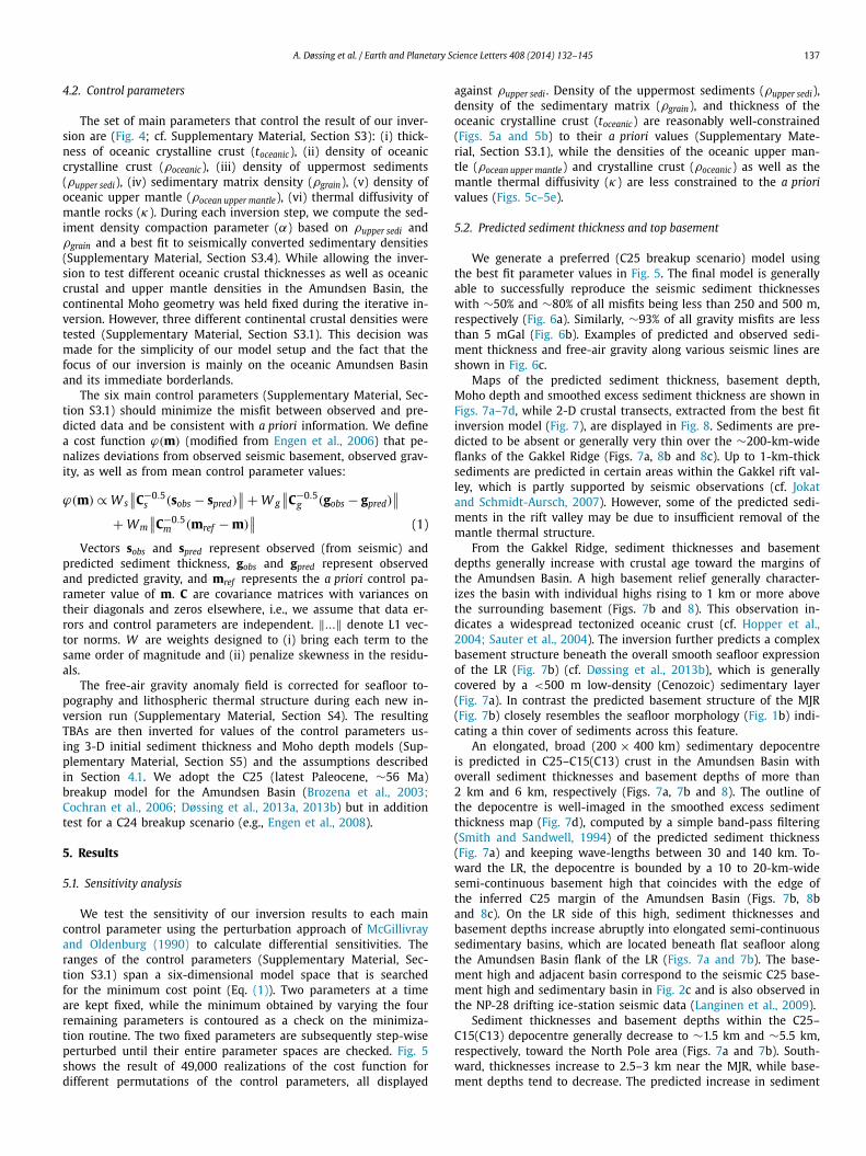
4.2. Control parameters

The set of main parameters that control the result of our inver-sion are (Fig. 4; cf. Supplementary Material, Section S3): (i) thick-ness of oceanic crystalline crust (toceanic), (ii) density of oceanic crystalline crust (ρoceanic), (iii) density of uppermost sediments (ρupper sedi), (iv) sedimentary matrix density (ρgrain), (v) density of oceanic upper mantle (ρocean upper mantle), (vi) thermal diffusivity of mantle rocks (κ ). During each inversion step, we compute the sed-iment density compaction parameter (α) based on ρupper sedi and ρgrain and a best fit to seismically converted sedimentary densities (Supplementary Material, Section S3.4). While allowing the inver-sion to test different oceanic crustal thicknesses as well as oceanic crustal and upper mantle densities in the Amundsen Basin, the continental Moho geometry was held fixed during the iterative in-version. However, three different continental crustal densities were tested (Supplementary Material, Section S3.1). This decision was made for the simplicity of our model setup and the fact that the focus of our inversion is mainly on the oceanic Amundsen Basin and its immediate borderlands.

The six main control parameters (Supplementary Material, Sec-tion S3.1) should minimize the misfit between observed and pre-dicted data and be consistent with a priori information. We define a cost function ϕ(m) (modified from Engen et al., 2006) that pe-nalizes deviations from observed seismic basement, observed grav-ity, as well as from mean control parameter values:

ϕ(m) ∝ W s∥∥C−0.5

s (sobs − spred)∥∥ + W g

∥∥C−0.5g (gobs − gpred)

∥∥+ Wm

∥∥C−0.5m (mref − m)

∥∥ (1)

Vectors sobs and spred represent observed (from seismic) and predicted sediment thickness, gobs and gpred represent observed and predicted gravity, and mref represents the a priori control pa-rameter value of m. C are covariance matrices with variances on their diagonals and zeros elsewhere, i.e., we assume that data er-rors and control parameters are independent. ‖...‖ denote L1 vec-tor norms. W are weights designed to (i) bring each term to the same order of magnitude and (ii) penalize skewness in the residu-als.

The free-air gravity anomaly field is corrected for seafloor to-pography and lithospheric thermal structure during each new in-version run (Supplementary Material, Section S4). The resulting TBAs are then inverted for values of the control parameters us-ing 3-D initial sediment thickness and Moho depth models (Sup-plementary Material, Section S5) and the assumptions described in Section 4.1. We adopt the C25 (latest Paleocene, ∼56 Ma) breakup model for the Amundsen Basin (Brozena et al., 2003;Cochran et al., 2006; Døssing et al., 2013a, 2013b) but in addition test for a C24 breakup scenario (e.g., Engen et al., 2008).

5. Results

5.1. Sensitivity analysis

We test the sensitivity of our inversion results to each main control parameter using the perturbation approach of McGillivray and Oldenburg (1990) to calculate differential sensitivities. The ranges of the control parameters (Supplementary Material, Sec-tion S3.1) span a six-dimensional model space that is searched for the minimum cost point (Eq. (1)). Two parameters at a time are kept fixed, while the minimum obtained by varying the four remaining parameters is contoured as a check on the minimiza-tion routine. The two fixed parameters are subsequently step-wise perturbed until their entire parameter spaces are checked. Fig. 5shows the result of 49,000 realizations of the cost function for different permutations of the control parameters, all displayed

against ρupper sedi . Density of the uppermost sediments (ρupper sedi), density of the sedimentary matrix (ρgrain), and thickness of the oceanic crystalline crust (toceanic) are reasonably well-constrained (Figs. 5a and 5b) to their a priori values (Supplementary Mate-rial, Section S3.1), while the densities of the oceanic upper man-tle (ρocean upper mantle) and crystalline crust (ρoceanic) as well as the mantle thermal diffusivity (κ ) are less constrained to the a priorivalues (Figs. 5c–5e).

5.2. Predicted sediment thickness and top basement

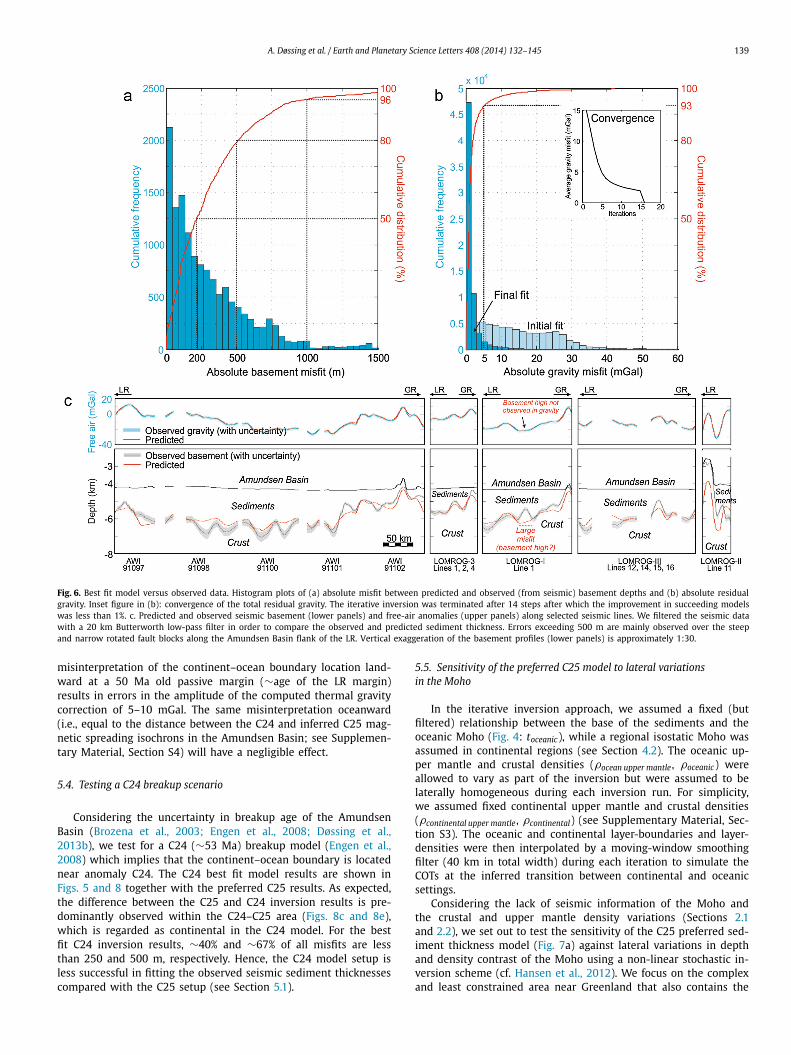
We generate a preferred (C25 breakup scenario) model using the best fit parameter values in Fig. 5. The final model is generally able to successfully reproduce the seismic sediment thicknesses with ∼50% and ∼80% of all misfits being less than 250 and 500 m, respectively (Fig. 6a). Similarly, ∼93% of all gravity misfits are less than 5 mGal (Fig. 6b). Examples of predicted and observed sedi-ment thickness and free-air gravity along various seismic lines are shown in Fig. 6c.

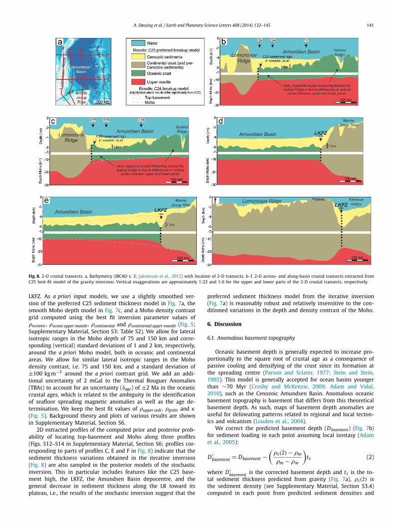
Maps of the predicted sediment thickness, basement depth, Moho depth and smoothed excess sediment thickness are shown in Figs. 7a–7d, while 2-D crustal transects, extracted from the best fit inversion model (Fig. 7), are displayed in Fig. 8. Sediments are pre-dicted to be absent or generally very thin over the ∼200-km-wide flanks of the Gakkel Ridge (Figs. 7a, 8b and 8c). Up to 1-km-thick sediments are predicted in certain areas within the Gakkel rift val-ley, which is partly supported by seismic observations (cf. Jokat and Schmidt-Aursch, 2007). However, some of the predicted sedi-ments in the rift valley may be due to insufficient removal of the mantle thermal structure.

From the Gakkel Ridge, sediment thicknesses and basement depths generally increase with crustal age toward the margins of the Amundsen Basin. A high basement relief generally character-izes the basin with individual highs rising to 1 km or more above the surrounding basement (Figs. 7b and 8). This observation in-dicates a widespread tectonized oceanic crust (cf. Hopper et al., 2004; Sauter et al., 2004). The inversion further predicts a complex basement structure beneath the overall smooth seafloor expression of the LR (Fig. 7b) (cf. Døssing et al., 2013b), which is generally covered by a <500 m low-density (Cenozoic) sedimentary layer (Fig. 7a). In contrast the predicted basement structure of the MJR (Fig. 7b) closely resembles the seafloor morphology (Fig. 1b) indi-cating a thin cover of sediments across this feature.

An elongated, broad (200 × 400 km) sedimentary depocentre is predicted in C25–C15(C13) crust in the Amundsen Basin with overall sediment thicknesses and basement depths of more than 2 km and 6 km, respectively (Figs. 7a, 7b and 8). The outline of the depocentre is well-imaged in the smoothed excess sediment thickness map (Fig. 7d), computed by a simple band-pass filtering (Smith and Sandwell, 1994) of the predicted sediment thickness (Fig. 7a) and keeping wave-lengths between 30 and 140 km. To-ward the LR, the depocentre is bounded by a 10 to 20-km-wide semi-continuous basement high that coincides with the edge of the inferred C25 margin of the Amundsen Basin (Figs. 7b, 8b and 8c). On the LR side of this high, sediment thicknesses and basement depths increase abruptly into elongated semi-continuous sedimentary basins, which are located beneath flat seafloor along the Amundsen Basin flank of the LR (Figs. 7a and 7b). The base-ment high and adjacent basin correspond to the seismic C25 base-ment high and sedimentary basin in Fig. 2c and is also observed in the NP-28 drifting ice-station seismic data (Langinen et al., 2009).

Sediment thicknesses and basement depths within the C25–C15(C13) depocentre generally decrease to ∼1.5 km and ∼5.5 km, respectively, toward the North Pole area (Figs. 7a and 7b). South-ward, thicknesses increase to 2.5–3 km near the MJR, while base-ment depths tend to decrease. The predicted increase in sediment

138 A. Døssing et al. / Earth and Planetary Science Letters 408 (2014) 132–145

Fig. 5. Sensitivity analysis. Inversion for control parameter values minimizing the cost function for real data. A priori values of control parameters (Supplementary Material, Section S3: Table S2) are shown by red lines. Inverted best fit (minimum cost) parameters for the preferred C25 opening model are shown by red dots. Background: contour plots of minimum costs for the C25 model setup. Density of upper sediments (ρupper sedi) vs. (a) sedimentary matrix density (ρgrain), (b) thickness of oceanic crystalline crust (toceanic), (c) density of oceanic upper mantle (ρocean upper mantle), (d) density of oceanic crystalline crust (ρoceanic), (e) thermal diffusivity of mantle rocks (κ ).

thickness is supported by Duckworth and Baggeroer (1985), who report more than 2-km-thick sediments in oceanic crust just to the north of the MJR. The thickening of the depocentre (Fig. 7a) culminates in a 250-km-long and up to 50-km-wide basin imme-diately north of – and parallel to – the edge of the MJR. Here, sediment thicknesses and basement depths are predicted to reach more than 3 km and 7 km, respectively (Figs. 7a, 7b, 8d and 8e). This elongated basin terminates abruptly against steeply rising basement of the MJR (in places more than 5 km over a distance of 30–50 km) and generally has the greatest basement depths just north of here. Interestingly, the inversion predicts a direct corre-lation of this basin with thick sediments (∼3–3.5 km) and deep basement (∼6.5 km) located against the LR in the Klenova Val-ley (Figs. 7a and 8f). The overall arcuate-shaped outline of these anomalously thick sediments correlate with the proposed loca-tion of the Eurekan LKFZ (see Fig. 1b) (cf. Brozena et al., 2003;Døssing et al., 2013b).

5.3. Sources of error

Small sedimentary misfits (<250 m) are generally observed beneath the flat abyssal plain of the Amundsen Basin and in ar-eas with a relatively smooth seabed (Fig. 6c). The greatest de-viations (>500 m) between interpreted (from seismic) and pre-dicted sediment thicknesses are generally found along the steep flanks of the LR (Fig. 6c: GEUS-LOMROG2009 Line 11) where the sharp and large-amplitude seafloor relief produced by rotated fault blocks (cf. Cochran et al., 2006) is not fully resolved by gravity. Here, the crustal density, Moho depth, and upper man-tle temperature are also expected to vary substantially. Further,

the Earth model (Fig. 4) assumes a simple crustal structure over-lain by homogeneous, low-density (Cenozoic) sediments. The as-sumption of a single sedimentary layer is not valid in all conti-nental areas where the gravity basement in places is likely com-prised by densified Mesozoic sediments (e.g., Jokat et al., 1992;Jackson et al., 2010). However, in accordance with seismic obser-vations (Jackson et al., 2010), almost no low-density sediments are predicted above crystalline continental basement (e.g., at the plateau of the LR; Fig. 7a). Elsewhere in inferred continental set-tings, notably in areas of the LR with Mesozoic sediments, the predicted sediment thicknesses may be too large.

The inversion is also sensitive to positional errors, unmapped structures, and errors in the bathymetric and gravimetric data set. We use the IBCAO v. 3.0 bathymetric data set of the Arctic Ocean (Jakobsson et al., 2012), which is based on a compilation of multi- and single-beam data, vintage submarine single-beam data, and digitized contours from published regional-scale bathymetric charts. Parts of the study area are still sparsely surveyed, and the quality and density of bathymetric soundings vary with a tendency of decreasing resolution toward Greenland. Similarly, the quality and resolution of the gravity data set (Fig. 3a) decrease signifi-cantly outside the LOMGRAV-09 area (see inset figure in Fig. 3a).

Finally, using a computationally fast 1-D plate cooling model (see Supplementary Material, Section S4), rather a 2-D or 3-D cool-ing model that incorporates lateral heat transfer, introduces errors in the thermal gravity correction, mainly at the COTs (Chappell and Kusznir, 2008b). However, the errors due to a 1-D cooling model are generally small for mature margins like the LR, and in the ocean centre, the errors are negligible (Chappell and Kusznir, 2008b). Chappell and Kusznir (2008b) further show that a 25 km

A. Døssing et al. / Earth and Planetary Science Letters 408 (2014) 132–145 139

Fig. 6. Best fit model versus observed data. Histogram plots of (a) absolute misfit between predicted and observed (from seismic) basement depths and (b) absolute residual gravity. Inset figure in (b): convergence of the total residual gravity. The iterative inversion was terminated after 14 steps after which the improvement in succeeding models was less than 1%. c. Predicted and observed seismic basement (lower panels) and free-air anomalies (upper panels) along selected seismic lines. We filtered the seismic data with a 20 km Butterworth low-pass filter in order to compare the observed and predicted sediment thickness. Errors exceeding 500 m are mainly observed over the steep and narrow rotated fault blocks along the Amundsen Basin flank of the LR. Vertical exaggeration of the basement profiles (lower panels) is approximately 1:30.

misinterpretation of the continent–ocean boundary location land-ward at a 50 Ma old passive margin (∼age of the LR margin) results in errors in the amplitude of the computed thermal gravity correction of 5–10 mGal. The same misinterpretation oceanward (i.e., equal to the distance between the C24 and inferred C25 mag-netic spreading isochrons in the Amundsen Basin; see Supplemen-tary Material, Section S4) will have a negligible effect.

5.4. Testing a C24 breakup scenario

Considering the uncertainty in breakup age of the Amundsen Basin (Brozena et al., 2003; Engen et al., 2008; Døssing et al., 2013b), we test for a C24 (∼53 Ma) breakup model (Engen et al., 2008) which implies that the continent–ocean boundary is located near anomaly C24. The C24 best fit model results are shown in Figs. 5 and 8 together with the preferred C25 results. As expected, the difference between the C25 and C24 inversion results is pre-dominantly observed within the C24–C25 area (Figs. 8c and 8e), which is regarded as continental in the C24 model. For the best fit C24 inversion results, ∼40% and ∼67% of all misfits are less than 250 and 500 m, respectively. Hence, the C24 model setup is less successful in fitting the observed seismic sediment thicknesses compared with the C25 setup (see Section 5.1).

5.5. Sensitivity of the preferred C25 model to lateral variations in the Moho

In the iterative inversion approach, we assumed a fixed (but filtered) relationship between the base of the sediments and the oceanic Moho (Fig. 4: toceanic), while a regional isostatic Moho was assumed in continental regions (see Section 4.2). The oceanic up-per mantle and crustal densities (ρocean upper mantle , ρoceanic) were allowed to vary as part of the inversion but were assumed to be laterally homogeneous during each inversion run. For simplicity, we assumed fixed continental upper mantle and crustal densities (ρcontinental upper mantle , ρcontinental) (see Supplementary Material, Sec-tion S3). The oceanic and continental layer-boundaries and layer-densities were then interpolated by a moving-window smoothing filter (40 km in total width) during each iteration to simulate the COTs at the inferred transition between continental and oceanic settings.

Considering the lack of seismic information of the Moho and the crustal and upper mantle density variations (Sections 2.1and 2.2), we set out to test the sensitivity of the C25 preferred sed-iment thickness model (Fig. 7a) against lateral variations in depth and density contrast of the Moho using a non-linear stochastic in-version scheme (cf. Hansen et al., 2012). We focus on the complex and least constrained area near Greenland that also contains the

140 A. Døssing et al. / Earth and Planetary Science Letters 408 (2014) 132–145

Fig. 7. Maps of results. a. Predicted sediment thickness. b. Predicted crystalline basement depth. Color-coded seismic calibration points in (a) and (b) are overlain for comparison. c. Predicted Moho depth. Colored dots in (c): color-coded seismic refraction Moho calibration points taken from the LOREX and LORITA profiles. The northern most Moho depths of the LORITA profile were not included, since these are poorly constrained (Jackson et al., 2010). d. Predicted (smoothed) excess sediment thickness (see text for details). The map images the outline of the Amundsen Basin depocentre with excess sediments of up to 800 m relative to surrounding oceanic areas. The arrows show the interpreted bottom currents responsible for the broad sediment thickness anomalies in the Amundsen Basin (modified from Kristoffersen et al., 2004). Cross-hatched signature in (a)–(d): areas where the inversion is expected to be uncertain due to sharp changes in bathymetry and/or low-resolution in the gravity.

A. Døssing et al. / Earth and Planetary Science Letters 408 (2014) 132–145 141

Fig. 8. 2-D crustal transects. a. Bathymetry (IBCAO v. 3; Jakobsson et al., 2012) with location of 2-D transects. b–f. 2-D across- and along-basin crustal transects extracted from C25 best-fit model of the gravity inversion. Vertical exaggerations are approximately 1:22 and 1:6 for the upper and lower parts of the 2-D crustal transects, respectively.

LKFZ. As a priori input models, we use a slightly smoothed ver-sion of the preferred C25 sediment thickness model in Fig. 7a, the smooth Moho depth model in Fig. 7c, and a Moho density contrast grid computed using the best fit inversion parameter values of ρoceanic , ρocean upper mantle , ρcontinental and ρcontinental upper mantle (Fig. 5; Supplementary Material, Section S3: Table S2). We allow for lateral isotropic ranges in the Moho depth of 75 and 150 km and corre-sponding (vertical) standard deviations of 1 and 2 km, respectively, around the a priori Moho model, both in oceanic and continental areas. We allow for similar lateral isotropic ranges in the Moho density contrast, i.e. 75 and 150 km, and a standard deviation of ±100 kg m−3 around the a priori contrast grid. We add an addi-tional uncertainty of 2 mGal to the Thermal Bouguer Anomalies (TBAs) to account for an uncertainty (δage) of ±2 Ma in the oceanic crustal ages, which is related to the ambiguity in the identification of seafloor spreading magnetic anomalies as well as the age de-termination. We keep the best fit values of ρupper sedi , ρgrain and κ(Fig. 5). Background theory and plots of various results are shown in Supplementary Material, Section S6.

2D extracted profiles of the computed prior and posterior prob-ability of locating top-basement and Moho along three profiles (Figs. S12–S14 in Supplementary Material, Section S6; profiles cor-responding to parts of profiles C, E and F in Fig. 8) indicate that the sediment thickness variations obtained in the iterative inversion (Fig. 8) are also sampled in the posterior models of the stochastic inversion. This in particular includes features like the C25 base-ment high, the LKFZ, the Amundsen Basin depocentre, and the general decrease in sediment thickness along the LR toward its plateau, i.e., the results of the stochastic inversion suggest that the

preferred sediment thickness model from the iterative inversion (Fig. 7a) is reasonably robust and relatively insensitive to the con-ditioned variations in the depth and density contrast of the Moho.

6. Discussion

6.1. Anomalous basement topography

Oceanic basement depth is generally expected to increase pro-portionally to the square root of crustal age as a consequence of passive cooling and densifying of the crust since its formation at the spreading centre (Parson and Sclater, 1977; Stein and Stein, 1992). This model is generally accepted for ocean basins younger than ∼70 Myr (Crosby and McKenzie, 2009; Adam and Vidal, 2010), such as the Cenozoic Amundsen Basin. Anomalous oceanic basement topography is basement that differs from this theoretical basement depth. As such, maps of basement depth anomalies are useful for delineating patterns related to regional and local tecton-ics and volcanism (Louden et al., 2004).

We correct the predicted basement depth (Dbasement) (Fig. 7b) for sediment loading in each point assuming local isostasy (Adam et al., 2005):

D ′basement = Dbasement −

(ρs(z̄) − ρm

ρm − ρw

)ts (2)

where D ′basement is the corrected basement depth and ts is the to-

tal sediment thickness predicted from gravity (Fig. 7a), ρs(z̄) is the sediment density (see Supplementary Material, Section S3.4) computed in each point from predicted sediment densities and

142 A. Døssing et al. / Earth and Planetary Science Letters 408 (2014) 132–145

Fig. 9. Anomalous basement. Map of computed anomalous basement depth �Dbasement (see text for details). Cross-hatched signature: areas where the inver-sion is expected to be uncertain due to sharp changes in bathymetry and/or low-resolution in the gravity.

averaged over the entire sedimentary column using 100 m in-tervals, ρm is the best fit oceanic upper mantle density, and ρw

is the density of water. The expected (unloaded) basement depth (Dtheoretical) is the basement predicted by a model of conductive cooling of the underlying lithosphere as a function of its age. Here, we use the crustal age model of the Amundsen Basin (Sup-plementary Material, Section S4) and the GDH1 oceanic thermal subsidence model of Stein and Stein (1992), with an assumed zero age depth of 2600 m. We compute the anomalous basement to-pography (�Dbasement) by removing Dtheoretical from the sediment-corrected basement (D ′

basement):

�Dbasement = D ′basement − Dtheoretical. (3)

Fig. 9 shows the computed �Dbasement for the oceanic Amund-sen Basin. Note that the amplitude and width of the interpreted C25 basement high along the LR (cf. Figs. 2c, 8b and 8c) increases markedly toward the LKFZ at the LR–MJR corner of the Amund-sen Basin. Here, a total elevated basement depth of ∼1200 m is predicted relative to the depressed basement in the centre of the Amundsen Basin. Fig. 9 also highlights another distinct basement high, which is parallel to the northern edge of the MJR. This high separates the broad Amundsen Basin depocentre and deep base-ment to the north from the deep elongated sedimentary basin pre-dicted along the LKFZ immediately north of the MJR (see Figs. 7a and 9). The high is 20 to 50-km-wide and characterized by anoma-lous basement depths of up to ∼700 m relative to the centre of the Amundsen Basin.

Fig. 10. Eurekan compression north of Greenland. a. Model of the plate tectonic configuration at 45 Ma following significant Eurekan compression (modified from Døssing et al., 2013b). Note the LKFZ transpressional to compressional structure against the LR and the nascent Amundsen Basin. Bold red line: Location of pro-file shown in (b). b. Interpreted crustal transect along the LR, Klenova Valley and MJR based on the extracted Profile F in Fig. 8. Note the suggested interpretation of a possible accretionary wedge at LKFZ in the Klenova Valley. Vertical exaggeration for the cross-section in (b) is approximately 1:22.

6.2. Eurekan compression north of Greenland

Based on the interpretation of new magnetic and gravity data, Døssing et al. (2013b) suggest that significant Eurekan transpression-to-compression took place along the more than 600-km-long offshore LKFZ, which they correlate with the onshore Eurekan Mount Rawlinson Fault in Ellesmere Island. The results of our inversions (Fig. 7) confirm the location of the LKFZ as a dis-tinct line of thick sediments and deep basement, notably north of the MJR and in the Klenova Valley against the LR (Figs. 8d–8f). In accordance with Døssing et al. (2013b) we further suggest that the predicted patterns of anomalous basement topography (Fig. 9), in particular the southward increase in amplitude and width of the C25 basement high as well as the smaller basement ridge just north of the MJR, are products of oceanic crustal formation during Eurekan N–S compression along the LKFZ. The compres-sion resulted in deformation of nascent oceanic crust against the LKFZ and may also have been responsible for creating the over-all bowl-shaped deep basement structure in the centre of the Amundsen Basin (Fig. 9). We tentatively suggest that Eurekan com-pression caused uplift and crustal shortening of the LR against the LKFZ and thereby contributed to the formation of the promi-nent plateau of the LR near Greenland (Fig. 10b) (cf. Døssing et al., 2013b). This interpretation is based on the bathymetric outline of the LR, being shallowest against the LKFZ (Fig. 1b), the overall southward predicted thinning of low-density (Cenozoic) sediments and the crustal thickening along the crest of the ridge toward the plateau (Figs. 8f and 10b). The above model for the plateau con-tradicts the purely magmatic origin as suggested by Jackson et al.(2010).

A. Døssing et al. / Earth and Planetary Science Letters 408 (2014) 132–145 143

6.3. The MJR volcanic province – a product of compression?

The outline of the MJR is clearly observed by high-amplitude positive magnetic anomalies (Døssing et al., 2010, 2013b), which probably image a large volcanic province. No samples have been dredged from the MJR but Tegner et al. (2011b, 2011a) suggest that the province is part of the alkaline volcanic rocks of the Kap Washington Group in North Greenland. These rocks possibly formed during latest Cretaceous (71.2 ± 0.5 Ma; 40Ar–39Ar dat-ing) continental rifting and further show a thermal resetting age of ∼49 Ma, which has been attributed to peak-Eurekan deforma-tion (Tegner et al., 2011b, 2011a; Døssing et al., 2013b). However, recent geochemical and radiometric dating results from dredged in situ rocks from the offshore Yermak Plateau, which is the conjugate to the MJR (Brozena et al., 2003), indicate stretched continental crust that is strongly affected by alkaline magmatism that formed around 51 Ma (Riefstahl et al., 2013). The age for the offshore Yermak Plateau magmatism potentially constrains the age of the MJR volcanism and correlates with the peak age of Eurekan de-formation in North Greenland (cf. Tegner et al., 2011b, 2011a). In accordance with Brozena et al. (2003), we therefore suggest that the MJR volcanism mainly formed during peak-Eurekan de-formation at the LKFZ. This interpretation further implies that the MJR volcanism took place in a state of compression at the LKFZ between an extended continental margin to the south and the ac-tive Gakkel spreading centre to the north (Fig. 10a). Interestingly, Riefstahl et al. (2013) find an anomalous geochemical signature in the rock samples from the Yermak Plateau which they attribute to Caledonian age subduction in the area. Could this signature relate to Eurekan tectonics instead, i.e., seafloor subduction and possibly even subduction of the actively spreading Gakkel Ridge at the LKFZ? This would imply mantle upwelling continuing within a slab window beneath a lithospheric plate after ridge subduc-tion (Thorkelson, 1996) and may provide a possible explanation for the magmatism within the highly extended continental crust of the MJR and the Yermak Plateau. Similar ridge subduction took place for the Cocos–Nazca spreading ridge segments from about 7 to 2 Ma beneath Central America (Johnston and Thorkelson, 1997)and is currently occurring for the Chile Ridge, which is subduct-ing beneath southern South America (Russo et al., 2010). However, whether Eurekan subduction of Amundsen Basin crust – and in particular subduction of the Gakkel spreading centre – took place at the LKFZ is not resolved by our data.

6.4. A note on paleoceanography

Similar to oceanic basement depth, sediment thicknesses are expected to increase with crustal age (Louden et al., 2004; Engen et al., 2006). However, at smaller scales, sediment thickness is strongly controlled by the original structural configuration of the underlying basement (Louden et al., 2004). In addition, the general pattern can be modified substantially by bottom-currents (Faugères et al., 1993) and the availability of sediments, notably in the Arc-tic regions, where sediment input is affected by glaciations, pro-glacial outwash, and resulting gravity flows to the deep basin (Kristoffersen et al., 2004; Louden et al., 2004).

Based on vintage seismic data, collected mainly from drifting ice-stations, Kristoffersen et al. (2004) propose the existence of a submarine channel and an associated continuous sedimentary fan extending along the Amundsen Basin flank of the LR. This interpre-tation, however, is not entirely supported by the smoothed excess sediment thickness map (Fig. 7d). Rather, the elongated sedimen-tary basin, confined along the LR near the North Pole, appears to be separated from the broad pattern of relatively thick sedi-ments further south near Greenland. We suggest that the sedimen-tary basin near the North Pole relates to rifting during breakup,

since the LR in this area strikes perpendicular to the proposed slightly transtensional breakup stresses and therefore suffered from greatest extension (Brozena et al., 2003; Minakov et al., 2011;Døssing et al., 2013b). In contrast, Fig. 7d indicates that sediment input to the Amundsen Basin depocentre came from the topo-graphically confined Klenova Valley, which was probably fed from nearby high-standing sources such as the elevated LR plateau and the Lincoln Sea glacial shelf (cf. Kristoffersen et al., 2004). We suggest that the submarine channel south of ∼88◦N, observed in seismic data along the LR (Kristoffersen et al., 2004), acted as a sediment bypass channel from where sediments were dumped into the broad and thick depocentre of the Amundsen Basin.

7. Conclusions

We present the results of 3-D gravity inversion for predict-ing the sediment thickness and basement geometry within the Amundsen Basin and along its continental borderlands in the Arc-tic Ocean north of Greenland. Our study provides the first detailed insights into the crustal and basement structure in an area that is underexplored by seismic data due to ice-related limitations.

We adopt the recently published LOMGRAV-09 gravity compi-lation and follow a process-oriented iterative cycle approach, as-suming a fixed (but filtered) relationship between the base of the oceanic sedimentary layer and the oceanic Moho as well as a re-gional isostatic Moho in continental settings. The sensitivity of our results to lateral variations in depth and density contrast of the Moho is subsequently tested by a stochastic inversion.

• Our results are mainly limited by the lack of borehole informa-tion in the Arctic Ocean as well as the sparsity of high quality seismic data and the uncertainty in the bathymetric data in the study area, notably toward Greenland.

• Within its limitations, our results provide the first detailed model of the sedimentary thickness and basement geometry beneath the oceanic Amundsen Basin and the inferred conti-nental LR, MJR and Klenova Valley.

• Our preferred results, using a C25 breakup model for the Amundsen Basin, provide a superior fit to seismic data com-pared with results from a C24 breakup model.

• A very variable basement relief is predicted in the Amundsen Basin and beneath the LR and MJR.

• Elongated basins are predicted along the LR and interpreted as rift-related features, while a broad, ∼ 200 × 400 km depocen-tre is predicted in the central Amundsen Basin. The outline of this depocentre indicates main sediment transport from the Klenova Valley between the LR and MJR.

• A distinct fault zone (LKFZ) is predicted along the northern edge of the MJR, continuing south of the LR and beneath the Lincoln Sea Shelf. Thick sediments are predicted within the LKFZ and evidence is shown of deformed continental and oceanic crust on both sides of the fault zone. We suggest that pronounced Eurekan crustal shortening took place along the LKFZ, affecting pre-C13 crustal formation in the Amundsen Basin and possibly contributing to the uplift of the LR plateau as well as the excess volcanism over the MJR.

Acknowledgements

Thanks to T.M. Rasmussen (Luleå University of Technology, Sweden), Indridi Einarsson (DTU Space), Gabriel Strykowski (DTU Space) and Øyvind Engen (Statoil) for valuable discussions. We also thank Prof. Dietmar Müller and an anonymous reviewer for constructive and positive reviews. The paper is published with per-mission from the Geological Survey of Denmark and Greenland (GEUS).

144 A. Døssing et al. / Earth and Planetary Science Letters 408 (2014) 132–145

Appendix A. Supplementary material

Supplementary material related to this article can be found on-line at http://dx.doi.org/10.1016/j.epsl.2014.10.011.

References

Adam, C., Vidal, V., 2010. Mantle flow drives the subsidence of oceanic plates. Sci-ence 328 (5974), 83–85.

Adam, C., Vidal, V., Bonneville, A., 2005. MiFil: a method to characterize seafloor swells with application to the south central Pacific. Geochem. Geophys. Geosyst. 6 (1), Q01003.

Alvey, A., Gaina, C., Kusznir, N., Torsvik, T., 2008. Integrated crustal thickness map-ping and plate reconstructions for the high arctic. Earth Planet. Sci. Lett. 274 (3–4), 310–321.

Blaich, O.A., Faleide, J.I., Tsikalas, F., 2011. Crustal breakup and continent–ocean transition at South Atlantic conjugate margins. J. Geophys. Res., Solid Earth (1978–2012) 116 (B1).

Breivik, A., Verhoef, J., Faleide, J., 1999. Effect of thermal contrasts on gravity mod-eling at passive margins: results from the western Barents Sea. J. Geophys. Res. 104 (B7), 15293.

Brozena, J.M., Childers, V.A., Lawver, L.A., Gahagan, L.M., Forsberg, R., Faleide, J.I., Eld-holm, O., 2003. New aerogeophysical study of the Eurasia Basin and Lomonosov Ridge: implications for basin development. Geology 31 (9), 825–828.

Chappell, A., Kusznir, N., 2008a. An algorithm to calculate the gravity anomaly of sedimentary basins with exponential density–depth relationships. Geophys. Prospect. 56 (2), 249–258.

Chappell, A., Kusznir, N., 2008b. Three-dimensional gravity inversion for Moho depth at rifted continental margins incorporating a lithosphere thermal grav-ity anomaly correction. Geophys. J. Int. 174 (1), 1–13.

Cochran, J., Edwards, M., Coakley, B., 2006. Morphology and structure of the Lomonosov Ridge, Arctic Ocean. Geochem. Geophys. Geosyst. 7 (5), Q05019.

Crosby, A., McKenzie, D., 2009. An analysis of young ocean depth, gravity and global residual topography. Geophys. J. Int. 178 (3), 1198–1219.

De Paor, D., Bradley, D., Eisenstadt, G., Phillips, S., 1989. The Arctic Eurekan orogen: a most unusual fold-and-thrust belt. Geol. Soc. Am. Bull. 101 (7), 952–967.

Døssing, A., Stemmerik, L., Dahl-Jensen, T., Schlindwein, V., 2010. Segmentation of the eastern North Greenland oblique-shear margin – regional plate tectonic im-plications. Earth Planet. Sci. Lett. 292 (3–4), 239–253.

Døssing, A., Jackson, H., Matzka, J., Einarsson, I., Rasmussen, T., Olesen, A., Brozena, J., 2013a. On the origin of the Amerasia Basin and the High Arctic Large Ig-neous Province – results of new aeromagnetic data. Earth Planet. Sci. Lett. 363, 219–230.

Døssing, A., Hopper, J., Olesen, A., Halpenny, J., 2013b. New aerogeophysical results from the Arctic Ocean, north of Greenland: implications for Late Cretaceous rift-ing and Eurekan compression. Geochem. Geophys. Geosyst. 14 (10), 4044–4065.

Duckworth, G., Baggeroer, A., 1985. Inversion of refraction data from the Fram and Nansen Basins of the Arctic Ocean. Tectonophysics 114 (1), 55–102.

Engen, Ø., Frazer, L., Wessel, P., Faleide, J., 2006. Prediction of sediment thickness in the Norwegian–Greenland Sea from gravity inversion. J. Geophys. Res. 111 (B11), B11403.

Engen, Ø., Faleide, J.I., Dyreng, T.K., 2008. Opening of the Fram Strait gateway: a re-view of plate tectonic constraints. Tectonophysics 450 (1), 51–59.

Faugères, J.C., Mézerais, M.L., Stow, D.A., 1993. Contourite drift types and their dis-tribution in the North and South Atlantic Ocean basins. Sediment. Geol. 82 (1), 189–203.

Forsberg, R., Kenyon, S., 2004. Gravity and geoid in the Arctic region: the north-ern polar gap now filled. In: Proceedings of the Second International GOCE User Workshop ‘GOCE, the Geoid and Oceanography’. 8–10 March 2004, Fras-cati, Italy.

Forsyth, D., Mair, J., 1984. Crustal structure of the Lomonosov Ridge and the Fram and Makarov Basins near the North Pole. J. Geophys. Res. 89, 473–481.

Gaina, C., Werner, S., Saltus, R., Maus, S., 2011. Circum-Arctic mapping project: new magnetic and gravity anomaly maps of the Arctic. Mem. Geol. Soc. Lond. 35 (1), 39–48.

Gee, J., Kent, D., 2007. Source of oceanic magnetic anomalies and the geomagnetic polarity timescale. In: Kono, M. (Ed.), Geomagnetism, Treatise on Geophysics, vol. 5, pp. 455–507.

Glebovsky, V.Y., Astafurova, E.G., Chernykh, A.A., Korneva, M.A., Kaminsky, V.D., Poselov, V.A., 2013. Thickness of the Earth’s crust in the deep Arctic ocean: re-sults of a 3D gravity modeling. Russ. Geol. Geophys. 54, 247–262.

Hansen, T., Cordua, K., Looms, M., Mosegaard, K., 2012. Sippi: a Matlab toolbox for sampling the solution to inverse problems with complex prior information: Part 1 – Methodology. Comput. Geosci. 52, 470–480.

Hermann, T., Jokat, W., 2013. Crustal structure of the Boreas Basin and the Knipovich Ridge, 76◦N, in the North Atlantic. Geophys. J. Int. 193 (3), 1399–1414.

Hopper, J.R., Funck, T., Tucholke, B.E., Larsen, H.C., Holbrook, W.S., Louden, K.E., Shillington, D., Lau, H., 2004. Continental breakup and the onset of ultraslow seafloor spreading off Flemish Cap on the Newfoundland rifted margin. Geol-ogy 32 (1), 93–96.

Jackson, H.R., Dahl-Jensen, T., The LORITA Working Group, 2010. Sedimentary and crustal structure from the Ellesmere Island and Greenland continental shelves onto the Lomonosov Ridge, Arctic Ocean. Geophys. J. Int. 182 (1), 11–35.

Jakobsson, M., Marcussen, C., Party, L.S., 2008. Lomonosov Ridge off Greenland 2007 (LOMROG) – Cruise Report. Special Publication Geological Survey of Denmark and Greenland, Copenhagen, Denmark, 122 pp.

Jakobsson, M., Mayer, L., Coakley, B., Dowdeswell, J., Forbes, S., Fridman, B., Hod-nesdal, H., Noormets, R., Pedersen, R., Rebesco, M., et al., 2012. The Interna-tional Bathymetric Chart of the Arctic Ocean (IBCAO) Version 3.0. Geophys. Res. Lett. 39 (12), L12609.

Johnston, S.T., Thorkelson, D.J., 1997. Cocos–Nazca slab window beneath central America. Earth Planet. Sci. Lett. 146 (3), 465–474.

Jokat, W., Micksch, U., 2004. Sedimentary structure of the Nansen and Amundsen basins, Arctic Ocean. Geophys. Res. Lett. 31 (2).

Jokat, W., Schmidt-Aursch, M., 2007. Geophysical characteristics of the ultraslow spreading Gakkel Ridge, Arctic Ocean. Geophys. J. Int. 168 (3), 983–998.

Jokat, W., Uenzelmann-Neben, G., Kristoffersen, Y., Rasmussen, T., 1992. Lomonosov Ridge – a double-sided continental margin. Geology 20 (10), 887–890.

Jokat, W., Weigelt, E., Kristoffersen, Y., Rasmussen, T., Schöne, T., 1995a. New insights into the evolution of the Lomonosov Ridge and the Eurasia Basin. Geophys. J. Int. 122 (2), 378–392.

Jokat, W., Weigelt, E., Kristofferseq, Y., Rasmussen, T., Schöne, T., 1995b. New geo-physical results from the south-western Eurasian Basin (Morris Jesup Rise, Gakkel Ridge, Yermak Plateau) and the Fram Strait. Geophys. J. Int. 123 (2), 601–610.

Jokat, W., Ritzmann, O., Schmidt-Aursch, M., Drachev, S., Gauger, S., Snow, J., 2003. Geophysical evidence for reduced melt production on the Arctic ultra-slow Gakkel mid-ocean ridge. Nature 423, 962–965.

Kaminskii, V., Suprunenko, O., Suslova, V., 2011. The continental shelf of the Russian Arctic region: the state of the art in the study and exploration of oil and gas resources. Russ. Geol. Geophys. 52 (8), 760–767.

Kristoffersen, Y., Sorokin, M., Jokat, W., Svendsen, O., 2004. A submarine fan in the Amundsen Basin, Arctic Ocean. Mar. Geol. 204 (3), 317–324.

Langinen, A., Lebedeva-Ivanova, N., Gee, D., Zamansky, Y., et al., 2009. Correlations between the Lomonosov Ridge, Marvin Spur and adjacent basins of the Arctic Ocean based on seismic data. Tectonophysics 472 (1–4), 309–322.

Laske, G., Masters, G., 1997. A global digital map of sediment thickness. EOS Trans. AGU 78, F483.

Louden, K.E., Tucholke, B.E., Oakey, G.N., 2004. Regional anomalies of sediment thickness, basement depth and isostatic crustal thickness in the North Atlantic Ocean. Earth Planet. Sci. Lett. 224 (1), 193–211.

Lyberis, N., Manby, G., 1993. The West Spitsbergen Fold Belt: the result of Late Cretaceous–Palaeocene Greenland–Svalbard convergence? Geol. J. 28 (2), 125–136.

Marcussen, C.t.L.S.P., 2011. Lomonosov Ridge off Greenland (LOMROG II) – cruise report. In: Danmarks og Grønlands Geologiske Undersøgelse Rapport, vol. 106. 154 pp.

Marcussen, C.t.L.S.P., 2012. Lomonosov Ridge off Greenland (LOMROG III) – cruise report. In: Danmarks og Grønlands Geologiske Undersøgelse Rapport, vol. 119. 222 pp.

McGillivray, P., Oldenburg, D., 1990. Methods for calculating Fréchet derivatives and sensitives for the non-linear inverse problem: a comparative study. Geophys. Prospect. 38 (5), 499–524.

Minakov, A., Faleide, J., Glebovsky, V.Y., Mjelde, R., 2011. Structure and evolution of the northern Barents—Kara sea continental margin from integrated analysis of potential fields, bathymetry and sparse seismic data. Geophys. J. Int. 188 (1), 79–102.

Morgan, J., Blackman, D., 1993. Inversion of combined gravity and bathymetry data for crustal structure: a prescription for downward continuation. Earth Planet. Sci. Lett. 119 (1), 167–179.

Oakey, G.N., Stephenson, R., 2008. Crustal structure of the Innuitian region of Arctic Canada and Greenland from gravity modelling: implications for the Palaeogene Eurekan orogen. Geophys. J. Int. 173 (3), 1039–1063.

Ostenso, N., Wold, R., 1977. A seismic and gravity profile across the Arctic Ocean Basin. Tectonophysics 37 (1–3), 1–24.

Parker, R., 1973. The rapid calculation of potential anomalies. Geophys. J. R. Astron. Soc. 31 (4), 447–455.

Parson, B., Sclater, J.G., 1977. An analysis of the variation of ocean floor bathymetry and heat flow with age. J. Geophys. Res. 32, 803–827.

Peron-Pinvidic, G., Gernigon, L., Gaina, C., Ball, P., 2012a. Insights from the Jan Mayen system in the Norwegian–Greenland Sea – I. Mapping of a microcontinent. Geo-phys. J. Int. 191 (2), 385–412.

Peron-Pinvidic, G., Gernigon, L., Gaina, C., Ball, P., 2012b. Insights from the Jan Mayen system in the Norwegian–Greenland Sea – II. Architecture of a micro-continent. Geophys. J. Int. 191 (2), 413–435.

Riefstahl, F., Estrada, S., Geissler, W.H., Jokat, W., Stein, R., Kämpf, H., Dulski, P., Nau-mann, R., Spiegel, C., 2013. Provenance and characteristics of rocks from the Yermak Plateau, Arctic Ocean: petrographic, geochemical and geochronological constraints. Mar. Geol. 343, 125–145.

A. Døssing et al. / Earth and Planetary Science Letters 408 (2014) 132–145 145

Russo, R., VanDecar, J.C., Comte, D., Mocanu, V.I., Gallego, A., Murdie, R.E., 2010. Subduction of the Chile Ridge: upper mantle structure and flow. GSA Today 20 (9), 4–10.

Sauter, D., Mendel, V., Rommevaux-Jestin, C., Parson, L.M., Fujimoto, H., Mével, C., Cannat, M., Tamaki, K., 2004. Focused magmatism versus amagmatic spreading along the ultra-slow spreading Southwest Indian Ridge: evidence from TOBI side scan sonar imagery. Geochem. Geophys. Geosyst. 5 (10), Q10K09.

Smith, W., Sandwell, D., 1994. Bathymetric prediction from dense satellite altimetry and sparse shipboard bathymetry. J. Geophys. Res. 99 (B11), 21803–21824.

Srivastava, S.P., Tapscott, C.R., 1986. Plate kinematics of the North Atlantic. In: Vogt, P.R., Tucholke, B.E. (Eds.), The Geology of North America. Vol. M, The Western North Atlantic Region. Geological Society of North America, pp. 379–404.

Stein, C.A., Stein, S., 1992. A model for the global variation in oceanic depth and heat flow with lithospheric age. Nature 359 (6391), 123–129.

Tegner, C., Storey, M., Holm, P., Thorarinsson, S., Zhao, X., Lo, C., Knudsen, M., 2011a. Erratum to “Magmatism and Eurekan deformation in the High Arctic

Large Igneous Province: 40Ar–39Ar age of Kap Washington Group volcanics, North Greenland” [Earth Planet. Sci. Lett. 303 (2011), 203–214]. Earth Planet. Sci. Lett. 311, 195–196.

Tegner, C., Storey, M., Holm, P., Thorarinsson, S., Zhao, X., Lo, C., Knudsen, M., 2011b. Magmatism and Eurekan deformation in the High Arctic Large Igneous Province: 40Ar–39Ar age of Kap Washington Group volcanics, North Greenland. Earth Planet. Sci. Lett. 303, 203–214.

Thorkelson, D.J., 1996. Subduction of diverging plates and the principles of slab win-dow formation. Tectonophysics 255 (1), 47–63.

Watts, A.B., 2001. Isostasy and Flexure of the Lithosphere. Cambridge University Press.

Watts, A., Fairhead, J., 1999. A process-oriented approach to modeling the gravity signature of continental margins. Lead. Edge 18, 258–263.

Weber, J., 1979. The Lomonosov Ridge experiment: LOREX 79. EOS Trans. AGU 60 (42), 715–721.