the mortar boundary element method
TRANSCRIPT
The Mortar Boundary Element Method
A Thesis submitted for the degree of Doctor of Philosophy
by Martin Healey
School of Information Systems, Computing and Mathematics
Brunel University
March 2010
Abstract
This thesis is primarily concerned with the mortar boundary element method (mortarBEM). The mortar finite element method (mortar FEM) is a well established numericalscheme for the solution of partial differential equations. In simple terms the techniqueinvolves the splitting up of the domain of definition into separate parts. The problemmay now be solved independently on these separate parts, however there must be somesort of matching condition between the separate parts. Our aim is to develop and analysethis technique to the boundary element method (BEM).
The first step in our journey towards the mortar BEM is to investigate the BEM withLagrangian multipliers. When approximating the solution of Neumann problems on opensurfaces by the Galerkin BEM the appropriate boundary condition (along the boundarycurve of the surface) can easily be included in the definition of the spaces used. However,we introduce a boundary element Galerkin BEM where we use a Lagrangian multiplierto incorporate the appropriate boundary condition in a weak sense. This is the firststep in enabling us to understand the necessary matching conditions for a mortar typedecomposition.
We next formulate the mortar BEM for hypersingular integral equations representingthe elliptic boundary value problem of the Laplace equation in three dimensions (withNeumann boundary condition). We prove almost quasi-optimal convergence of the schemein broken Sobolev norms of order 1/2. Sub-domain decompositions can be geometricallynon-conforming and meshes must be quasi-uniform only on sub-domains.
We present numerical results which confirm and underline the theory presented con-cerning the BEM with Lagrangian multipliers and the mortar BEM. Finally we discuss theapplication of the mortaring technique to the hypersingular integral equation representingthe equations of linear elasticity. Based on the assumption of ellipticity of the appearingbilinear form on a constrained space we prove the almost quasi-optimal convergence ofthe scheme.
i
Contents
Abstract i
List of Figures v
List of Tables vi
Acknowledgements vii
1 Introduction 11.1 Overview of Thesis . . . . . . . . . . . . . . . . . . . . . . . . . . . . . . . 11.2 Background Information . . . . . . . . . . . . . . . . . . . . . . . . . . . . 2
1.2.1 The Boundary Element Method . . . . . . . . . . . . . . . . . . . . 21.2.2 Lagrangian Multipliers . . . . . . . . . . . . . . . . . . . . . . . . . 31.2.3 Mortar Methods . . . . . . . . . . . . . . . . . . . . . . . . . . . . 4
1.3 Notations . . . . . . . . . . . . . . . . . . . . . . . . . . . . . . . . . . . . 6
2 Mathematical Background 72.1 The Boundary Element Method . . . . . . . . . . . . . . . . . . . . . . . . 7
2.1.1 The Boundary Element Method . . . . . . . . . . . . . . . . . . . . 92.2 Mixed Finite Element Methods . . . . . . . . . . . . . . . . . . . . . . . . 13
2.2.1 The Finite Element Method . . . . . . . . . . . . . . . . . . . . . . 132.2.2 Nonconforming Formulation . . . . . . . . . . . . . . . . . . . . . . 152.2.3 Finite Element Method with Lagrangian Multiplier . . . . . . . . . 162.2.4 Babuska-Brezzi Theory . . . . . . . . . . . . . . . . . . . . . . . . . 182.2.5 Extension of Strang Type Estimate . . . . . . . . . . . . . . . . . . 192.2.6 The Mortar Finite Element Method . . . . . . . . . . . . . . . . . . 21
2.3 Technical Details . . . . . . . . . . . . . . . . . . . . . . . . . . . . . . . . 272.3.1 Surface Differential Operators . . . . . . . . . . . . . . . . . . . . . 272.3.2 Integration By Parts Formula . . . . . . . . . . . . . . . . . . . . . 302.3.3 Transformation To a Reference Sub-Domain . . . . . . . . . . . . . 32
ii
CONTENTS iii
2.3.4 Other Required Results . . . . . . . . . . . . . . . . . . . . . . . . . 35
3 The BEM with Lagrangian Multiplier 383.1 Towards a Discrete Formulation . . . . . . . . . . . . . . . . . . . . . . . . 38
3.1.1 Introduction and Model Problem . . . . . . . . . . . . . . . . . . . 383.1.2 Integration By Parts . . . . . . . . . . . . . . . . . . . . . . . . . . 403.1.3 Discrete Variational Formulation with Lagrangian Multiplier . . . . 41
3.2 Technical Results and Proof of the Main Result . . . . . . . . . . . . . . . 43
4 The Mortar Boundary Element Method 494.1 Towards a Discrete Formulation . . . . . . . . . . . . . . . . . . . . . . . . 49
4.1.1 Model Problem . . . . . . . . . . . . . . . . . . . . . . . . . . . . . 494.1.2 Sub-domain decomposition . . . . . . . . . . . . . . . . . . . . . . . 504.1.3 Integration by parts . . . . . . . . . . . . . . . . . . . . . . . . . . 54
4.2 Discrete Variational Formulation of the Mortar BEM . . . . . . . . . . . . 574.2.1 Meshes and Discrete Spaces . . . . . . . . . . . . . . . . . . . . . . 574.2.2 Setting of the Mortar Boundary Element Method . . . . . . . . . . 60
4.3 Technical Details and Proof of the Main Result . . . . . . . . . . . . . . . 61
5 Numerical Results 765.1 An Error Estimate . . . . . . . . . . . . . . . . . . . . . . . . . . . . . . . 765.2 BEM With Lagrangian Multiplier . . . . . . . . . . . . . . . . . . . . . . . 795.3 Mortar Boundary Element Method . . . . . . . . . . . . . . . . . . . . . . 81
5.3.1 Mortar BEM - Conforming Sub-Domain Decomposition . . . . . . . 815.3.2 Mortar BEM - Non-Conforming Sub-Domain Decomposition I . . . 875.3.3 Mortar BEM - Non-Conforming Sub-Domain Decomposition II . . . 93
6 Mortar BEM for Linear Elasticity 996.1 Background . . . . . . . . . . . . . . . . . . . . . . . . . . . . . . . . . . . 99
6.1.1 Linear Elasticity . . . . . . . . . . . . . . . . . . . . . . . . . . . . 996.1.2 Model problem . . . . . . . . . . . . . . . . . . . . . . . . . . . . . 1016.1.3 Integration By Parts Formula . . . . . . . . . . . . . . . . . . . . . 104
6.2 Technical Results and Proof of the Main Result . . . . . . . . . . . . . . . 115
7 Conclusions and Further Research 1297.1 Conclusions . . . . . . . . . . . . . . . . . . . . . . . . . . . . . . . . . . . 1297.2 Suggestions for further research . . . . . . . . . . . . . . . . . . . . . . . . 130
A Proof of Proposition 4.8 132

CONTENTS iv
B Tables Of Numerical Results 136
Bibliography 147
Index 152
List of Figures
2.1 An example of a domain decomposed into sub-domains . . . . . . . . . . . 23
4.1 Sub-domain decomposition examples. . . . . . . . . . . . . . . . . . . . . . 514.2 Interface examples. . . . . . . . . . . . . . . . . . . . . . . . . . . . . . . . 524.3 Lagrangian multiplier side examples. . . . . . . . . . . . . . . . . . . . . . 534.4 Examples of globally nonconforming but locally conforming meshes. . . . . 584.5 Definition of discrete Lagrangian multiplier space. . . . . . . . . . . . . . . 604.6 Construction of wl in the proof of Lemma 4.12. . . . . . . . . . . . . . . . 67
5.1 Uniform meshes Th and Gk. . . . . . . . . . . . . . . . . . . . . . . . . . . . 795.2 Relative error curves for the BEM with Lagrangian multiplier . . . . . . . 805.3 Choice of Lagrangian multiplier side for Experiment 1 . . . . . . . . . . . . 815.4 Different Lagrangian multiplier sides. . . . . . . . . . . . . . . . . . . . . . 825.5 Mortar BEM experiment 1 . . . . . . . . . . . . . . . . . . . . . . . . . . . 845.6 Mortar BEM experiment 2 . . . . . . . . . . . . . . . . . . . . . . . . . . . 855.7 Mortar BEM experiment 3 . . . . . . . . . . . . . . . . . . . . . . . . . . . 865.8 Different Lagrangian multiplier sides. . . . . . . . . . . . . . . . . . . . . . 875.9 Mesh refinement examples . . . . . . . . . . . . . . . . . . . . . . . . . . . 885.10 Mortar BEM experiment 4 . . . . . . . . . . . . . . . . . . . . . . . . . . . 905.11 Mortar BEM experiment 5 . . . . . . . . . . . . . . . . . . . . . . . . . . . 915.12 Mortar BEM experiment 6 . . . . . . . . . . . . . . . . . . . . . . . . . . . 925.13 Different Lagrangian multiplier sides . . . . . . . . . . . . . . . . . . . . . 935.14 Mesh refinement examples . . . . . . . . . . . . . . . . . . . . . . . . . . . 945.15 Mortar BEM experiment 7 . . . . . . . . . . . . . . . . . . . . . . . . . . . 965.16 Mortar BEM experiment 8 . . . . . . . . . . . . . . . . . . . . . . . . . . . 975.17 Mortar BEM experiment 9 . . . . . . . . . . . . . . . . . . . . . . . . . . . 98
A.1 Mesh example . . . . . . . . . . . . . . . . . . . . . . . . . . . . . . . . . . 132
v
List of Tables
B.1 Dimensions and mesh sizes for BEM with Lagrangian multiplier . . . . . . 137B.2 Dimensions and mesh sizes for mortar BEM experiment 1 . . . . . . . . . . 138B.3 Dimensions and mesh sizes for mortar BEM experiment 2 . . . . . . . . . . 139B.4 Dimensions and mesh sizes for mortar BEM experiment 3 . . . . . . . . . . 140B.5 Dimensions and mesh sizes for mortar BEM experiment 4 . . . . . . . . . . 141B.6 Dimensions and mesh sizes for mortar BEM experiment 5 . . . . . . . . . . 142B.7 Dimensions and mesh sizes for mortar BEM experiment 6 . . . . . . . . . . 143B.8 Dimensions and mesh sizes for mortar BEM experiment 7 . . . . . . . . . . 144B.9 Dimensions and mesh sizes for mortar BEM experiment 8 . . . . . . . . . . 145B.10 Dimensions and mesh sizes for mortar BEM experiment 9 . . . . . . . . . . 146
vi
Acknowledgements
I would like to thank the many people who have helped me during the preparation of thisthesis.
The first words of thanks must go to my supervisor Prof. Norbert Heuer, withoutwhom this thesis would never have been possible. Prof. Heuer has been a constant sourceof useful advice and encouragement, and it has been a privilege to work with him. I amespecially grateful for our correspondence over the last year which has taken place overquite a considerable distance.
I would also like to thank Prof. G Gatica for his assistance with Chapter 3, particularlywith the proof of Lemma 3.4. I must also thank Dr. M Maischak for his program MaiProgswhich was used as the basis for the programs used in Chapter 5.
I am also very grateful to my wife, Hazel, whose support has been invaluable. I wouldalso like to thank the rest of my family for their support.
I would like to thank the staff at Brunel University who have made my time at theuniversity enjoyable and stimulating.
vii
Chapter 1
Introduction
In this chapter we first present a brief overview of the thesis, indicating what is containedin each of the following chapters. We then present a brief discussion on the boundaryelement method (BEM) and related topics which are central to the thesis.
1.1 Overview of Thesis
In this chapter we present the motivation behind the research. We briefly discuss theadvantages (and disadvantages) of using techniques such as the BEM, non-conformingmethods, and domain decomposition methods. This discussion is intended to give aflavour of what follows and indicate the motivation behind the thesis.
Chapter 2 is split into two parts. In the first part we present the relevant backgroundinformation on the BEM, the finite element method (FEM) and some extensions to thebasic finite element method. Eventually we briefly present the mortar finite elementmethod (mortar FEM). We describe the formulation of the numerical scheme and discusssome of the theoretical results associated with the method. We also discuss some of theproblems which shall need to be overcome when translating the mortar FEM over to theboundary element situation. In the second part of the chapter we present a selection oftechnical results which are required for use in the later chapters. This section is intendedas a common point of reference for what follows.
In Chapter 3 we present the boundary element method with Lagrangian multiplier.We introduce the model problem and an integration by parts formula which we shall use toget the boundary terms required to introduce the Lagrangian multipliers. We then presentthe discrete variational formulation of the scheme (there is no continuous formulation),where we define the bilinear forms that we shall use and the necessary discrete spaces. Wethen present technical results which are steps on the way to proving our main theoremfor this chapter, the quasi-optimal convergence of the scheme.
1
CHAPTER 1. INTRODUCTION 2
In Chapter 4 we present the mortar boundary element method (mortar BEM). Weproceed in a similar fashion to the previous chapter. Of particular interest we clearlydefine the sub-domain decomposition that will be used. It is this ability to decompose thedomain into sub-domains that is the primary advantage of the mortar BEM over standardBEM schemes. We may mesh each sub-domain independently giving us great freedom inour choice of mesh. As noted we proceed in a similar fashion to the previous chapter,however now in a more complicated situation. We again show several technical resultswhich are required to prove our main theorem. Finally we present the main result of thechapter, the almost quasi-optimal convergence of the scheme in broken Sobolev norms.
In Chapter 5 we present numerical results for both the BEM with Lagrangian multi-plier and for the mortar BEM. These results are presented in graphical form in Chapter 5and also in numerical form in Appendix B. These numerical results confirm the theoryand present some interesting points in their own right. For example it is interesting to notethe effect of choice of Lagrangian multiplier side on the accuracy of the approximation.
In Chapter 6 we present some technical results for the mortar BEM applied to theequations of linear elasticity. This chapter is an extension of the previous work, showinghow the results obtained in previous chapters can be used in different situations. Inthis chapter we have had to include a conjecture related to the ellipticity of one of theappearing bilinear forms, since we were unable to prove this property. We explain whythere are difficulties and present some ideas about how the problem may be overcome.
1.2 Background Information
1.2.1 The Boundary Element Method
The analysis of finite elements for the discretisation of boundary integral equations ofthe first kind goes bank to Nedelec and Planchard [44], and Hsiao and Wendland [31].Stephan [53] studied boundary elements for singular problems on open surfaces. Stephanexamined the Laplace equations with Neumann boundary condition and reexpressed theproblem in terms of a hypersingular integral operator defined over the boundary. Theprinciple advantage of the BEM over other numerical methods like the FEM is that onlythe boundary of the domain needs to be discretised. However, there is a disadvantagewhich is that the matrices which appear in the BEM are full unlike in the FEM wherethey are sparse and banded (and hence can be solved very efficiently). More informationon the BEM (and the related integral equations) can, for example, be found in [32, 41] or[51].
CHAPTER 1. INTRODUCTION 3
1.2.2 Lagrangian Multipliers
Lagrangian multipliers where first analysed for the FEM by Babuska in [1]. The aim wasto be able to avoid difficulty in implementing essential boundary conditions. The basicidea is that through the inclusion of a second bilinear form we may use simpler spaces.As always there is however a trade off, although the spaces are simpler the associatedlinear system is larger and therefore more difficult to solve. A recent approach to the useof Lagrangian multipliers in terms of mixed finite elements is analysed in [2]. Lagrangianmultipliers are well known as a classical technique from variational methods.
While there is extensive use of Lagrangian multipliers in the FEM literature, there isno theory on the use of Lagrangian multipliers in the boundary element Galerkin method.There are several reasons why there is no such theory for the BEM:
• In the context of the FEM it has been shown that Lagrangian multiplier methodsare particularly useful for boundary value problems with nonhomogeneous Dirichletboundary conditions. By the inclusion of a second bilinear form we are able tosimplify the finite element spaces required to approximate a solution at the expenseof making the corresponding linear system larger. However, there are no boundaryvalue problems with representation by boundary integral equations where nonho-mogeneous boundary conditions (for the solution of the integral equations) appear.When examining the application of hypersingular operators on open surfaces bound-ary element function of a conforming method need to vanish at the boundary of thesurface [52]. As in the finite element case this homogeneous condition can be easilyincorporated into the method without the use of Lagrangian multipliers.
• In the finite element situation the analysis of Dirichlet boundary conditions is wellunderstood since there is a well defined trace operator for restricting functions overthe domain to the appropriate part of the boundary. When examining the appli-cation of hypersingular operators the analysis of essential boundary conditions ismuch more difficult due to the fact that there is no well defined trace operator inH1/2 (the critical space for hypersingular operators).
The existence of a weak treatment of boundary conditions for the FEM has led to manyuseful applications, such as non-conforming or discontinuous approximations. The weaktreatment of boundary conditions clearly shows us how to deal with interface conditions(either between elements or between sub-domains). In Chapter 3 we present a weaktreatment of boundary conditions for the BEM (previously such a weak treatment of theboundary conditions was unknown), which will open the door to new methods that arecurrently unknown for hypersingular integral operators. Some of these methods includenonconforming or discontinuous domain decomposition methods. The ideas also allowexamination of nonconforming or discontinuous elements,for example Crouzeix-Raviart
CHAPTER 1. INTRODUCTION 4
type (see [30]) or primal hybrid formulations. An extension of this analysis to mortar-type decompositions is shown in Chapter 4.
Essential properties of the analysis of the BEM of boundary integral equations ofthe first kind on open surfaces [52] include fractional order Sobolev spaces consisting offunctions which can be continuously extended by zero onto a larger surface. We note thatfor certain order Sobolev spaces this is not the same condition as enforcing a homogeneousboundary condition on the space. We aim to take this analysis to the next stage byanalysing and implementing this extendibility condition through the use of Lagrangianmultipliers. We thus shall provide the analysis for weak interface conditions in H1/2 andshow that they can be incorporated into discrete subspaces of H1/2 in an almost quasi-optimal way. A quasi-optimal error estimate is one that gives the convergence order of thebest approximation error (Cea’s Lemma). ”Quasi” comes from a factor in Ceas estimatewhich may be larger than one. We use the term ”almost quasi-optimal” for error estimateswhich are quasi-optimal up to a logarithmically growing factor. In Chapter 3 we considerthe model situation of homogeneous boundary conditions for the hypersingular operator(of the Laplacian) on an open surface.
1.2.3 Mortar Methods
The mortar method is a nonconforming Galerkin approximation scheme that can be clas-sified as a non-overlapping domain decomposition method. Domain decomposition tech-niques are well established for the FEM see [46] and [54] for an overview. We howeverwish to study the specific domain decomposition technique known as the mortar FEM.The mortar FEM is an extension of the Primal Hybrid FEM introduced in [47], wherethe constraint of inter-element continuity has been removed at the expense of introducinga Lagrangian multiplier. This allows a more general and less restrictive approach to theconstruction of finite element approximations. The mortar FEM was first introduced inthe early nineties in [5] and [6]. Although originally introduced with the aim of combiningspectral methods having different polynomial degrees, or the spectral method with theFEM it can however, as stated, be used as a domain decomposition technique for thefinite element method. The original paper has been followed by work by the original andother authors in many areas and extensions to the original ideas such as problems in threedimensions, preconditioning and a posteriori error estimates, see e.g. [3, 11, 12, 35, 36, 57]and [58] to cite a few. In particular, the hp-version and graded meshes have been studiedin [20] and [50]. Recent advances include the mortar method being applied to parabolicproblems [45].
The main attraction of the mortar method is to allow for different discretisations indifferent parts of the domain of the underlying problem. Different discretisations canresult from the use of either different meshes and/or different types of basis functions on
CHAPTER 1. INTRODUCTION 5
different parts of the domain. In the mortar method the compatibility of discretisationsacross interfaces of sub-domains is ensured only in a weak sense by some integral matchingcondition. This means that instead of having a continuous approximation over the wholeregion we will have discontinuities across interfaces in the approximating function. Thesediscontinuities will add to the error of the method, however this should be balanced by theability to get more accurate approximations in certain areas of the region. Alternativelyit may be a computational pay off: for example we may only require that the solution beaccurate in a certain part of the region and not in others so we can concentrate more onthat part by using a finer mesh.
Typical applications are in large scale simulations where substructures can be discre-tised separately. One example of this is in the modelling of an aeroplane where the mainbody and wings can be discretised separately. The advantages of this approach are thatwe can optimize our approximation for substructures, that we can solve different parts ofthe problem separately (e.g. on a parallel computer), and that the meshing of complicatedstructures can be made simpler by breaking the structure up into smaller parts which canthen be meshed more simply. This means that the mortar method allows us to tacklecomplicated large scale problems by decomposing the large problem into a collection ofsmaller, easier to solve sub-problems. In this way we can find approximations to problemswhich may not be possible or practical for standard approximations.
The mortar FEM generalizes to three dimensions, see for example [4, 10] or [35]. It isparticularly useful in three dimensions as a complex geometry can often be decomposedinto sub-geometries that are more easily meshed independently. The interfaces betweensub-domains in the three dimensional case are now two dimensional surfaces, compared tothe two dimensional mortar FEM where interfaces where simply one dimensional pieces.This means that unlike in the two dimensional case where we simply had non-conformityacross edges, in the three dimensional case we now have non-conformity across surfaces.This, obviously, makes things more complicated computationally in the three-dimensionalcase. We note that the continuity at cross points constraint that was originally imposed inthe two dimensional case now becomes the constraint of continuity along whole edges of theinterface in the three dimensional case. This is a severe constraint which would eliminatesome of the advantage of the mortar FEM. However as shown in [4] this condition, as inthe two dimensional case, can be relaxed to allow a less restrictive method.
Mortar boundary element method
Instead of the standard (conforming) boundary element formulation we shall study thedomain decomposition method known as the mortar method. We shall split the domainup into N non-overlapping sub-domains and require a weak compatibility condition onthe interfaces between sub-domains. We shall require a compatibility condition across
CHAPTER 1. INTRODUCTION 6
the interface between two sub-domains. This compatibility condition shall be expressedas an integral over the interface, and in order to produce this integral we require anintegration by parts formula. The weak compatibility condition will be incorporated by aLagrangian multiplier, which means that we require an appropriate integration by partsformula. The weak compatibility condition means that, unlike the standard BEM, ourapproximate solution may not be continuous across the whole domain (although it iscontinuous on each sub-domain).
To be precise, we apply the mortar technique directly to the boundary element dis-cretisation, not as a coupling procedure between boundary and finite elements as in [17].We follow the analysis presented in [3] (and briefly outlined in Section 2.2.6) for the mor-tar FEM, where projection and extension operators are used to bound the error in thekernel space (of functions satisfying the Lagrangian multiplier condition). Note that thereis a shorter presentation by Braess, Dahmen and Wiener [11] where the simpler argument[9, Remark III.4.6] is used to bound this error by a standard approximation error (inun-restricted spaces). Nevertheless, in our case the Strang-type error estimate has a morecomplicated structure and it is not straightforward to follow the argument [9, RemarkIII.4.6]. In particular our more complicated structure arises from the lack of a continuousformulation of the mortar scheme.
1.3 Notations
Notations. The symbols ”.” and ”&” will be used in the usual sense. In short, ah(v) .
bh(v) when there exists a constant C > 0 independent of the discretisation parameter hsuch that ah(v) ≤ Cbh(v). The double inequality ah(v) . bh(v) . ah(v) is simplified toah(v) ≃ bh(v). In our case the generic constant C is also independent of the fractionalSobolev index ǫ > 0.
In Chapters 2-5 we will also use the notation vj for the restriction of a function vto the sub-domain Γj. Chapter 6 uses a slightly different notation which is discussed onpage 99.
Chapter 2
Mathematical Background
This chapter is split into three distinct parts. In Section 2.1 we begin by briefly presentingthe BEM for the Laplace equation. The next step is to discuss the existence and unique-ness of the solution to the proposed scheme and finally to present an error estimate forthe scheme.
In Section 2.2 we shall briefly introduce and discuss the non-conforming FEM, themixed formulation of the FEM and the mortar FEM. We shall pay particular attentionto the areas where there are problems in the translation of the method from the finiteelement situation to the boundary element situation. We also present some well knownresults which are required for the existence and uniqueness of the solution to the methodswhich we propose.
In Section 2.3 we shall show some results which are needed for the application of themortar method to the boundary element situation. We first introduce an integration byparts formula for the problem, followed by some results relating to the surface differentialoperators used in the integration by parts formula and finally we present some otherresults which shall be required for the following chapters. This section is intended as apoint of common reference for the following chapters.
2.1 The Boundary Element Method
Before presenting the BEM we briefly present some of the spaces and norms which willbe required.
Sobolev spaces
In the following we let Ω ⊂ IRn be a domain (or surface when n = 2) with Lipschitzboundary ∂Ω. We first define the following spaces:
7

CHAPTER 2. MATHEMATICAL BACKGROUND 8
C(Ω) space of continuous functions in Ω,Ck(Ω) space of k times continuously differentiable functions in Ω,C∞(Ω) space on infinitely many times continuously differentiable functions in Ω,C∞
0 (Ω) space of functions from C∞(Ω) with compact support.
We now briefly define the needed Sobolev spaces. Let (the Lebesgue integral) of a(suitably smooth and well defined) function v be defined by
‖v‖L2(Ω) :=
(∫
Ω
|v(x)|2 dx
)1/2
.
We then define the Lebesgue space
L2(Ω) :=v : ‖v‖L2(Ω) <∞
,
and the product space(L2(Ω))2 := L2(Ω) × L2(Ω).
For positive integer k we define the norm in Hk(Ω) as
‖u‖Hk(Ω) :=
∫
Ω
∑
|α|≤k
|Dαu(x)|2 dx
1/2
.
Where we have used the multi-index α := (α1, . . . , αn) (in n dimensions), that |α| :=∑ni=1 αi and that Dα := ( ∂
∂x1) · · · ( ∂
∂xn). We may then define the space Hk(Ω) as:
Hk(Ω) closure of C∞(Ω) under the norm ‖u‖Hk(Ω).
We also define the space
H1loc(Ω) := u a distribution in Ω : u ∈ H1(Ω ∩BR)∀R > 0,
where BR is the open ball with centre the origin and radius R, and a distribution is ageneralised function which allows us to differentiate functions whose derivatives do notexist in a classical sense. We now define the space
H10 (Ω) := v ∈ L2(Ω); ∇v ∈ (L2(Ω))2, v = 0 on ∂Ω.
Where ∇v is the gradient of v defined by (in n dimensions)
∇v = grad v =
(∂u
∂xi
)n
i=1
in Ω.
We may also define H10 (Ω) as
CHAPTER 2. MATHEMATICAL BACKGROUND 9
H10 (Ω) closure of C∞
0 (Ω) under the norm ‖u‖H1(Ω).
We consider standard Sobolev spaces where the following norms are used: For 0 <s < 1 we define
‖u‖2Hs(Ω) := ‖u‖2
L2(Ω) + |u|2Hs(Ω) (2.1)
with semi-norm
|u|Hs(Ω) :=(∫
Ω
∫
Ω
|u(x) − u(y)|2
|x− y|2s+ndx dy
)1/2
. (2.2)
We then define the space
Hs(Ω) completion of C∞(Ω) under the norm ‖u‖Hs(Ω).
For a Lipschitz domain Ω and 0 < s < 1 we have the norm
‖u‖Hs(Ω) :=(|u|2Hs(Ω) +
∫
Ω
u(x)2
(dist(x, ∂Ω))2sdx)1/2
. (2.3)
We then define the space
Hs(Ω) completion of C∞(Ω) under the norm ‖u‖Hs(Ω).
For s ∈ (0, 1/2), ‖ · ‖Hs(Ω) and ‖ · ‖Hs(Ω) are equivalent norms whereas for s ∈ (1/2, 1)
there holds Hs(Ω) = Hs0(Ω), the latter space being the completion of C∞
0 (Ω) with norm inHs(Ω). Also we note that functions from Hs(Ω) are continuously extendable by zero ontoa larger domain. For all these results we refer to [26, 38]. For s > 0 the spaces H−s(Ω) andH−s(Ω) are the dual spaces of Hs(Ω) and Hs(Ω), respectively. Fractional order Sobolevspaces can be equivalently defined by interpolation, details on the real K-method may befound in [41, Appendix B].
2.1.1 The Boundary Element Method
The hypersingular integral equation
We consider the problem of the screen surface Γ. For a given function g on Γ we wish tofind u in Ω := IR3 \ Γ satisfying
− ∆u = 0 in Ω (2.4)
∂u
∂n= g on Γ and (2.5)
u = o(r−1) as r := |x| → ∞. (2.6)
CHAPTER 2. MATHEMATICAL BACKGROUND 10
Where ∆ is the Laplace operator given by
∆u =∂2u
∂x21
+∂2u
∂x22
+∂2u
∂x23
,
where x = (x1, x2, x3) ∈ IR3 are Cartesian coordinates. We also require the normalderivative of a function w defined by
∂w
∂n= n · ∇w =
∂w
∂x1
n1 +∂w
∂x2
n2 +∂w
∂x3
n3 on ∂Ω.
Here, n = (n1, n2, n3) denotes the exterior unit normal vector along ∂Ω.Further we assume that Γ is a bounded, simply connected, orientable, smooth, open
surface in IR3 with a smooth boundary curve γ which does not intersect itself. Our solutionprocedure is to derive boundary integral equations of the first kind on Γ for the jump ofthe field [u] across Γ. This is expressed in the following theorem.
Theorem 2.1. [53, Theorem 2.6] u ∈ H1loc(Ω) is the solution of the screen Neumann prob-
lem (2.4) - (2.6) if and only if the jump [u]|Γ ∈ H1/2(Γ) is the solution of the hypersingularintegral equation
−1
4π
∫
Γ
[u](y)∂2
∂nx∂ny
1
|x− y|dSy = g(x)
for x ∈ Γ and given g ∈ H−1/2(Γ).
Model problem
For simplicity let Γ be the plane open surface with polygonal boundary, and we shalldenote its boundary by ∂Γ. We shall identify the surface Γ with a subset of IR2, thusreferring to Γ as a domain rather than a surface and also referring to sub-domains of Γrather than sub-surfaces. Now our model problem is: For a given f ∈ H−1/2(Γ) find
φ ∈ H12 (Γ) such that
Wφ(x) := −1
4π
∂
∂nx
∫
Γ
φ(y)∂
∂ny
1
|x− y|dSy = f(x), x ∈ Γ. (2.7)
Here, n is a normal unit vector on Γ, e.g. n = (0, 0, 1)T . We note that the hypersingularoperator W maps H1/2(Γ) continuously onto H−1/2(Γ) (see [19], [53]).
We have the following weak (variational) formulation of (2.7). Find φ ∈ H12 (Γ) such
thata(φ, ψ) := 〈Wφ,ψ〉Γ = 〈f, ψ〉Γ =: F (ψ) ∀ψ ∈ H1/2(Γ). (2.8)
CHAPTER 2. MATHEMATICAL BACKGROUND 11
Here, 〈·, ·〉Γ denotes the L2(Γ) inner product and is also used for its generic extension byduality (e.g. between H−1/2(Γ) and H1/2(Γ)). Later we will indicate just the supportwhere the duality is taken (e.g. Γ or its boundary γ). Here also, a(·, ·) is a bilinear formand F (·) is a linear form.
To define the boundary element space we consider a triangulation Th = Kj : j =1, . . . ,m of Γ into polygons (or elements) Kj, which are typically triangles or rectangles,i.e.
Γ =⋃
K∈Th
K.
Here we assume that any two polygons are disjoint or intersect at a single vertex or anentire edge. The triangulation Th is also called a mesh on Γ. Our boundary element spaceis then
Xh := ψh ∈ C0(Γ) : ψh|K ∈ P r(K)∀K ∈ Th, ψh|∂Γ = 0, r ≥ 1
where Γ is the closure of Γ, P r(K) denotes the set of polynomials defined in K and ofdegree less than or equal to r, ψh|K denotes the restriction of vh to the element K, andsimilarly ψh|∂Γ denotes the restriction of ψh to ∂Γ. In two dimensions the maximumdiameter of the element K is denoted by h and is known as the mesh size parameter.
A standard Galerkin BEM for the approximate solution of (2.8), is to select a piecewise
polynomial subspace Xh ⊂ H12 (Γ) and define an approximant φh ∈ Xh by
a(φh, ψ) := 〈Wφh, ψ〉Γ = 〈f, ψ〉Γ =: F (ψ) ∀ψ ∈ Xh.
We note that to arrive at the weak formulation we simply multiply by a test functionand integrate over the boundary. This is different to the FEM where we require anintegration by parts formula (see Section 2.2.1 later) to arrive at the weak formulationwhich in turn provides us with the necessary boundary integrals to be able to incorporatea Lagrangian multiplier and thus develop the mortar FEM. No such integration by partsformula is used to generate the weak form of the BEM as the restriction to the boundary(of the boundary) of the functions in the test space for the BEM is not well defined (see thetrace theorem later Lemma 2.22 ). This means that there is no immediately obvious termto use as a Lagrangian multiplier and hence generate a mortar BEM. We thus have to finda different way of representing the formulation so that we can incorporate a Lagrangianmultiplier.
Existence and uniqueness of solution
We now consider the existence and uniqueness of the solution to the following more generalproblem
Find u ∈ V such that a(u, v) = F (v) ∀v ∈ V. (2.9)

CHAPTER 2. MATHEMATICAL BACKGROUND 12
Where V is a Hilbert space with the associated norm ‖ · ‖V . With the approximation
Find uh ∈ Vh such that a(uh, v) = F (v) ∀v ∈ Vh. (2.10)
Where Vh is an appropriately chosen discrete space.
Definition 2.2. We have the following:
• The linear form F (·) : V → IR is called continuous (or bounded) if
∃C > 0 : |F (v)| ≤ C‖v‖V ∀v ∈ V.
• The bilinear form a(·, ·) : V × V → IR is called continuous (or bounded) if
∃Cα > 0 : |a(v, w)| ≤ Cα‖v‖V ‖w‖V ∀v, w ∈ V.
• The bilinear form a(·, ·) : V × V → IR is called V-elliptic (or simply elliptic orcoercive) if
∃α > 0 : |a(v, v)| ≥ α‖v‖2V ∀v ∈ V.
We now state the well known Lax-Milgram Theorem which guarantees existence anduniqueness of the solution. For a proof of the Theorem see e.g. [14, Section 2.7].
Theorem 2.3. (Lax-Milgram) Let V be a Hilbert space, a(·, ·) a continuous V -ellipticbilinear form and F (·) a continuous linear form on V. Then (2.9) has a unique solutionv ∈ V .
We now state the following result on the error of the approximation of the problem.For a proof of the Theorem see e.g. [14, Section 2.8].
Theorem 2.4. (Cea) Let a(·, ·) be a continuous V -elliptic bilinear form and F (·) ∈ V ′
(V ′ is the dual space of V ). Then, for Vh ⊂ V the solution u ∈ V of (2.9) and uh ∈ Vh of(2.10) satisfy
‖u− uh‖V ≤Cαα
‖u− v‖V ∀v ∈ V, (2.11)
where Cα is the continuity constant and α is the ellipticity constant of a(·, ·) on V .
CHAPTER 2. MATHEMATICAL BACKGROUND 13
Error estimate
Now returning to our weak formulation (2.8) we see that V = H1/2(Γ) is a Hilbert space,and that the bilinear form a(·, ·) is both continuous (on V ) and V -elliptic, and that F (·)is a continuous linear form on V . We thus have, by the Lax-Milgram theorem (Theorem2.3), the existence and uniqueness of a solution to this formulation. We now considerthe discrete approximation (2.11) and note that since Vh ⊂ V the necessary assumptionson the bilinear and linear forms immediately follow. Again, the Lax-Milgram theorem(Theorem 2.3) gives us the existence and uniqueness of a solution to this formulation. Thisanalysis now implies the necessary conditions for the application of Cea’s lemma (Theorem2.4), which gives us a suitable bound on the error of our approximation, through the useof standard approximation theory.
The solution φ of (2.8) has strong corner and corner-edge singularities such that φ 6∈H1(Γ) in general, see [56]. A refined error analysis for the conforming BEM yields forquasi-uniform meshes an optimal error estimate
‖φ− φh‖H1/2(Γ) ≤ C h1/2,
see [8] or [33]. Such an error analysis makes use of an explicit knowledge of the appearingsingularities. When using only the Sobolev regularity φ ∈ H1−ǫ(Γ) with ǫ > 0, standardapproximation theory proves
‖φ− φh‖H1/2(Γ) ≤ C h1/2−ǫ‖φ‖H1−ǫ(Γ).
2.2 Mixed Finite Element Methods
In this section we briefly introduce the FEM for the Poisson equation. We then discusssome alternative formulations such as nonconforming formulations, the FEM with La-grangian multiplier and the mortar FEM. We also introduce some of the theory whichwill be required to prove existence and uniqueness to the solutions of these formulationsas well as provide us with an error estimate for them.
2.2.1 The Finite Element Method
In this section we will give a brief presentation of the derivation of the FEM for thePoisson equation with homogeneous Dirichlet boundary condition. For more details werefer to [9, 14, 18, 22] and [34]. We shall examine the Poisson equation with homogeneousDirichlet boundary condition on a bounded Lipschitz domain Ω ⊂ IR2:
− ∆u = f in Ω,
CHAPTER 2. MATHEMATICAL BACKGROUND 14
u = 0 on ∂Ω. (2.12)
Where f is a given function, ∂Ω denotes the boundary of Ω. The Laplace operator canbe rewritten in the following form
∆u = div∇u,
and div is the divergence defined for a vector valued function A = (A1, A2) by (in twodimensions)
divA =∂A1
∂x1
+∂A2
∂x2
in Ω.
Let us now recall the following integration by parts formula.
Lemma 2.5 (First Green formula). For sufficiently smooth functions v and A = (A1, A2)there holds ∫
Ω
∇v ·A dx =
∫
∂Ω
vn ·A ds−
∫
Ω
v · divA dx
The first integral on the right-hand side denotes integration with respect to arc length salong ∂Ω.
Now multiplying the Poisson equation by a sufficiently smooth function v, integratingover Ω and using the first Greens formula we get
∫
Ω
fv dx =
∫
Ω
−∆u v dx =
∫
Ω
∇u · ∇v dx−
∫
∂Ω
∂u
∂nv ds. (2.13)
Now, selecting the space V := H10 (Ω) we see that the boundary term in (2.13) (the
integral over ∂Ω) is equal to zero for v ∈ Vh. This leads to the following weak formulationof the Laplace equation
Find u ∈ V such that a(u, v) = F (v) ∀v ∈ V (2.14)
witha(u, v) := 〈∇u,∇v〉Ω and F (v) := 〈f, v〉Ω. (2.15)
The finite element method (FEM) for the solution of (2.12) consists of solving(2.14) with a finite dimensional subspace Vh of V . This finite element space is constructedby piecewise polynomial functions, as we did in the BEM. We may choose the followingspace:
Vh := vh ∈ C0(Ω) : vh|K ∈ P r(K)∀K ∈ Th, vh|∂Ω = 0, r ≥ 1.
CHAPTER 2. MATHEMATICAL BACKGROUND 15
The FEM for (2.12) then reads
Find uh ∈ Vh such that a(uh, vh) = F (v) ∀vh ∈ Vh. (2.16)
Appropriate ellipticity and continuity properties may be shown for the forms above. Thusexistence and uniqueness of solution follows from Theorem 2.3, and an error estimate canbe obtained using Theorem 2.4 and standard approximation theory.
2.2.2 Nonconforming Formulation
We shall now consider the situation when our discrete space is not a subset of our con-tinuous space. By this we mean that
Vh 6⊂ V.
One example of such a discrete space being chosen is where we choose a finite dimensionalspace that does not satisfy the specified boundary conditions. In (2.14) and (2.16) wehad Vh ⊂ V = H1
0 (Ω). This means that our discrete functions satisfy the homogeneousboundary condition by the choice of the discrete space. If instead of this we chooseVh ⊂ H1(Ω) 6⊂ V i.e. our discrete functions do not satisfy the homogeneous boundarycondition we find that we can still apply the Lax-Milgram Theorem (Theorem 2.3) to getexistence and uniqueness of the solution but we can no longer appeal to Cea’s Theorem(Theorem 2.4) for our error estimate. Instead we must appeal to the Second StrangLemma. For a proof of the Lemma see e.g. [14, Section 10.1].
Lemma 2.6. (Strang) Let V and Vh be subspaces of a Hilbert space H. Assume that a(·, ·)is a continuous bilinear form defined on H which is Vh-elliptic, with respective continuityand ellipticity constants Cα and α. Let u ∈ V solve
a(u, v) = F (v) ∀v ∈ V,
where F ∈ H ′. Let uh ∈ Vh solve
a(uh, v) = F (v) ∀v ∈ Vh.
Then
‖u− uh‖H ≤
(1 +
Cαα
)infv∈Vh
‖u− v‖H +1
αsup
w∈Vh\0
|a(u− uh, w)|
‖w‖H. (2.17)
The second term on the right-hand side of (2.17) would be zero if Vh ⊂ V . Thereforethis term measures the degree of nonconformity in the approximation.
CHAPTER 2. MATHEMATICAL BACKGROUND 16
2.2.3 Finite Element Method with Lagrangian Multiplier
Lagrangian multipliers are a convenient method for the inclusion of nonhomogeneousessential boundary conditions into the FEM. They allow us to drop the constraint on thespace at the expense of including a second bilinear form. The early work on applying thismethod to the FEM is presented in [1], and a more recent examination is shown in [2].The approximation of the boundary conditions through the use of a Lagrangian multipliermay be considered as the simplest formulation of the mortar FEM, where we only haveone sub-domain.
We shall now examine the Poisson equation with nonhomogeneous Dirichlet (essential)boundary condition on a bounded Lipschitz domain Ω ⊂ IR2:
− ∆u = f in Ω,
u = g on ∂Ω. (2.18)
Where g is a given function. As before we multiply by a suitable function v, integrateover Ω and apply the first Greens formula to get (2.13). Now, selecting the space X as
X := H1(Ω)
we see that by choosing u, v ∈ X in (2.13) we do not have the situation where the boundaryterm disappears (we do not have the homogeneous boundary condition included in thedefinition of our space). We may now define the bilinear form a(·, ·) and the linear formF (·) as in (2.15). We also define the bilinear form b(·, ·) and the linear form G(·) as
b(v, λ) =
∫
∂Ω
λv ds
G(v) =
∫
∂Ω
gv ds.
In the bilinear form b(·, ·) above we have λ = ∂u∂n
, this is our Lagrangian multiplier term.We now define the space M (the dual space of the trace space of X) as
M := (H1/2(∂Ω))′ = H−1/2(∂Ω).
The above spaces lead to the following weak formulation with Lagrangian multiplier ofthe Laplace equation with nonhomogeneous Dirichlet boundary condition. Find (u, λ) ∈X ×M such that
a(u, v) + b(λ, v) = F (v) ∀v ∈ X
CHAPTER 2. MATHEMATICAL BACKGROUND 17
b(u, ψ) = G(ψ) ∀ψ ∈M. (2.19)
Where G(ψ) is a linear form mapping M onto IR. We see that when compared to the weakformulation of the Laplace equation with nonhomogeneous boundary conditions we haveused simpler spaces X = H1(Ω) rather than V g = v ∈ H1(Ω); v = g on ∂Ω. Howeverthis comes at the expense of the introduction of a second bilinear form b(·, ·) and theintroduction of a second space M . The bilinear form b(·, ·) imposes the nonhomogeneousboundary condition in a weak sense. By this we mean that we only require that oursolution u satisfies an integral matching condition rather than explicitly stating in thedefinition of the space that u = g on ∂Ω. The space M is referred to as the Lagrangianmultiplier space and its members are referred to as Lagrangian multipliers.
To arrive at this continuous formulation required two items of particular interest whentranslating to the boundary element situation. Firstly, we required an integration by partsformula which defined a suitable boundary term that can be used as an interface matchingcondition. Secondly we require the use of the Trace Theorem for the restriction of functionsfrom the domain to the boundary. These are two central issues for the translation fromthe FEM to the BEM situation.
The finite element method with Lagrangian multiplier for the solution of (2.19)is Find (uh, λk) ∈ Xh ×Mk such that
a(uh, v) + b(λk, v) = F (v) ∀v ∈ Xh
b(uh, ψ) = G(ψ) ∀ψ ∈Mk. (2.20)
Where Xh and Mk are finite dimensional subspaces of X and M respectively.Of particular interest to us shall be a situation similar to the homogeneous Dirichlet
boundary condition case. We see that in this case (i.e. g = 0) we would have the followingformulation: Find (u, λ) ∈ X ×M such that
a(u, v) + b(λ, v) = F (v) ∀v ∈ X
b(u, ψ) = 0 ∀ψ ∈M. (2.21)
If we now introduce the space
V := v ∈ X : b(v, ψ) = 0 ∀ψ ∈M. (2.22)
We arrive at the equivalent formulation: Find u ∈ V such that
a(u, v) = F (v) ∀v ∈ V. (2.23)
CHAPTER 2. MATHEMATICAL BACKGROUND 18
Existence and uniqueness results for the finite element method with Lagrangian mul-tiplier follow from the Babuska-Brezzi Theory which shall be detailed below. An errorestimate for the method can be obtained through an extension of the Strang-type estimate,which shall also be detailed below.
As explained before, when examining the application of hypersingular operators onopen surfaces boundary element functions of a conforming method need to vanish at theboundary of the surface. This homogeneous condition can be easily incorporated into themethod through the definition of the space, and the use of simple approximating functions.However, for our mortar method we do not want the approximating functions to vanish atthe interface between sub-domains (since the function being approximated does not). Thistheory gives us an indication of the direction in which to head for an error estimate forour method.
2.2.4 Babuska-Brezzi Theory
We have the following Theorem for the continuous problem defined in (2.19). For a proofsee e.g. [48, Theorem 10.1].
Theorem 2.7. Let the bilinear form a(·, ·) be continuous on X ×X and V -elliptic, i.e.
infv∈V :‖v‖V =1
a(v, v) > 0. (2.24)
Also, let the bilinear form b(·, ·) is continuous on M × V and that it satisfies
infv∈X:‖v‖X=1
supψ∈M :‖ψ‖M=1
b(ψ, v) > 0. (2.25)
Then for each pair of continuous linear forms F (·) on X and G(·) on M , problem (2.19)has a unique solution.
Remark 2.8. Condition (2.25) is often referred to as the inf-sup condition. It is alsoreferred to as the Brezzi-condition, the Babuska-Brezzi condition, or the LBB condition(where the L refers to Ladyzhenskaya). See [49] for an interesting discussion on the namingof this condition.
We also have the following Theorem for the discrete situation. For a proof see e.g.[48, Theorem 10.1].
Theorem 2.9. Let the bilinear form a(·, ·) be Vh-elliptic, let the bilinear form b(·, ·) satisfy
infvh∈Xh:‖vh‖X=1
supψh∈Mh:‖ψh‖M=1
b(ψh, vh) > 0. (2.26)
Then for each pair of linear forms F (·) on Xh and G(·) on Mh, problem (2.20) has aunique solution.

CHAPTER 2. MATHEMATICAL BACKGROUND 19
Remark 2.10. Condition (2.26) is called the discrete inf-sup condition or the discreteLBB condition. It says that the choice of the subspaces Xh of X and Mh of M cannot bemade independently of one another, and that there is a compatibility condition betweenthe two subspaces.
The Babuska-Brezzi theory can be viewed as a generalisation of the Lax-Milgramtheory to the mixed formulation. Condition (2.26) can be equivalently expressed as
∃β > 0 : infµ∈Mh
supv∈Xh
b(v, µ)
‖µ‖M‖v‖X≥ β.
or
∃β > 0 : supv∈Xh
b(v, µ)
‖v‖X≥ β‖µ‖M ∀µ ∈Mh.
Here the constant β is known as the inf-sup constant.In order to apply this Babuska-Brezzi theory to our proposed methods we need to show
the necessary properties of the bilinear forms. For a continuous formulation we wouldhave to show that the bilinear form a(·, ·) is continuous on X × X and V -elliptic andthat the bilinear form b(·, ·) is continuous on M × V . While some of the properties woulddirectly cross over to the discrete case for the bilinear form a(·, ·) it is worth noting thatsince in general Vh 6⊂ V such properties related to these spaces would not directly transfer.
2.2.5 Extension of Strang Type Estimate
We shall now examine the mixed formulation (2.21). We shall seek an approximatesolution to (2.21) using the following discrete formulation: Find (uh, λh) ∈ Xh×Mh suchthat
a(uh, vh) + b(λh, vh) = F (vh) ∀vh ∈ Xh
b(uh, ψh) = 0 ∀ψh ∈Mh. (2.27)
We now define the space
Vh = vh ∈ Xh : b(vh, ψh) = 0 ∀ψh ∈Mh. (2.28)
Now we have the equivalent formulation (to (2.27)): Find uh ∈ Vh such that
a(uh, vh) = F (vh) ∀vh ∈ Vh. (2.29)
CHAPTER 2. MATHEMATICAL BACKGROUND 20
We recall the Strang type estimate (Lemma 2.6) where the second term on the right handside of (2.17) is a measure of the non-conformity of the method. We shall now examinethis second term, which is
1
αsup
w∈Vh\0
|a(u− uh, w)|
‖w‖M.
For w ∈ Vh,
a(u− uh, w) = a(u,w) − a(uh, w)= a(u,w) − F (w)= −b(w, λ)= −b(w, λ− ψ) ∀ψ ∈Mh. (2.30)
We note that this requires the existence of a continuous formulation to hold, specificallywe require that
a(u,w) + b(w, λ) = F (w),
where u ∈ X is our continuous solution and since w ∈ Vh ⊂ Xh ⊂ X. Now if the bilinearform b(·, ·) is continuous we have that
|b(w, λ− ψ)| ≤ ‖w‖X‖λ− ψ‖M . (2.31)
Combining (2.30) and (2.31) gives us that
|a(u− uh, w)| ≤ ‖w‖X‖λ− ψ‖M .
We now have the following bound on the error, for a proof see e.g. [14, Theorem 12.3.7].
Theorem 2.11. Let Xh ⊂ X and Mh ⊂ M , and define Vh and V by (2.22) and (2.28)respectively. Assume that the bilinear form a(·, ·) is both V and Vh-elliptic. Assume thatthe bilinear form b(·, ·) is continuous on X ×M with constant C. Let u and λ be definedby (2.21), and let uh be defined by (2.27)(or equivalently (2.29)). Then
‖u− uh‖X ≤
(1 +
Cαα
)infv∈Vh
‖u− v‖X +C
αinf
ψ∈Mh\0‖λ− ψ‖M . (2.32)
As in Lemma 2.6 we have two parts to our error estimate. The second term representsthe degree of nonconformity in the method as before only this time it is clear that thecontribution stems from the Lagrangian multipliers.
In order to apply this Strang-type theory to our proposed methods we would requireboth a continuous and a discrete formulation. Not having a continuous formulation wouldcomplicate matters, although would not need to be an obstacle.
CHAPTER 2. MATHEMATICAL BACKGROUND 21
2.2.6 The Mortar Finite Element Method
We shall follow the procedure as described in [3] for the presentation of the mortar FEM.The conforming sub-domain decomposition will be shown for ease of presentation. Weshall discuss the two dimensional case as this has the most relevance to our boundaryelement case.
We break up the initial domain Ω ⊂ IR2 into N non-overlapping sub-domains Ωi,1 ≤ i ≤ N , which are assumed to be polygonally shaped. They are arranged suchthat any two sub-domains are disjoint or intersect at a single vertex or an entire edge.This is known as a geometrical conforming decomposition. A geometrical non-conformingdecomposition occurs where two sub-domains intersect along part of an edge, but notnecessarily the whole edge. The mortar FEM can be extended to the non-conformingcase (of sub-domain decomposition), but we shall deal with the conforming case here forthe sake of simplicity. We thus have that
Ω =N⋃
i=1
Ωi, Ωi ∩ Ωj = ∅ for i 6= j
Whenever two sub-domains Ωi and Ωj, i < j, are adjacent, Γij is the common interface,
Γij = Ωi ∩ Ωj.
For simplicity let i denote the set of all indices j so that ij exists and i is the class of allindices j ∈ i with j > i. We denote by nij the unit normal orientated from Ωi towardsΩj and we set nij = −nji. We also have that the Γij form a skeleton, S
S :=N⋃
i=1
⋃
j∈i
Γij
Continuous formulation
We need the following space:
X :=v ∈ L2(Ω) : v|Ωi
∈ H1(Ωi), i = 1, . . . , N, v|∂Ω = 0,
endowed with the norm
‖v‖X :=
(N∑
i=1
‖v‖2H1(Ωi)
)1/2
.
Having split the original domain up into sub-domains we now apply our integrationby parts formula, Lemma 2.5, on each sub-domain individually to get the following for
CHAPTER 2. MATHEMATICAL BACKGROUND 22
u, v ∈ X ∫
Ωi
∇u · ∇v dx =
∫
Ωi
fv dx+
∫
∂Ωi
∂u
∂nv ds.
Now summing over all sub-domains, recalling the homogeneous boundary conditionon the original domain (which has been included in the space X), we have the followingweak mixed continuous formulation: Find (u, λ) ∈ X ×M such that for f ∈ L2(Ω)
a(u, v) + b(v, λ) = F (v) ∀v ∈ X
b(u, µ) = 0 ∀µ ∈M (2.33)
where
a(u, v) =N∑
i=1
∫
Ωi
∇u · ∇v dx =N∑
i=1
〈∇u,∇v〉Ωi(2.34)
b(v, µ) =∑
Γij⊂S
∫
Γij
µ[v] dSx =∑
Γij⊂S
〈µ, [v]〉Γij(2.35)
F (v) = 〈f, v〉Ω (2.36)
where [v] is the jump of v ∈ X , it is defined on the skeleton S by [v] := v|Ωk− v|Ωl
onΓkl. Note that each interface Γkl appears only once in the sum over S. We note that thenormal derivative is a mapping H1(Ωi) → H−1/2(∂Ωi).
We can thus define the Lagrangian multiplier space M as
M :=∏
Γij⊂S
H−1/2(Γij),
with the associated norm
‖ψ‖M :=
N∑
i=1
∑
j∈i
‖ψ‖2H−1/2(Γij)
1/2
.
We note that for each Γij the indexing order is important, for Γij, Ωi is the non-mortar side. This fact, the distinction between mortar and non-mortar side, is veryimportant when considering a non-conforming sub-domain decomposition. Analysis ofthe continuous problem leads to the jump over Γij being [v] ∈ H1/2(Γij) (the dual spaceof H−1/2(Γij)). This means that in particular we require that the jump vanishes at theend points of the interface.
CHAPTER 2. MATHEMATICAL BACKGROUND 23
We place the matching conditions into the definition of our space in the following way
V := v ∈ X : b(v, µ) = 0∀µ ∈M .
We thus arrive at the following equivalent formulation of the weak continuous problem:Find u ∈ V such that
a(u, v) = F (v) ∀v ∈ V. (2.37)
Discrete formulation
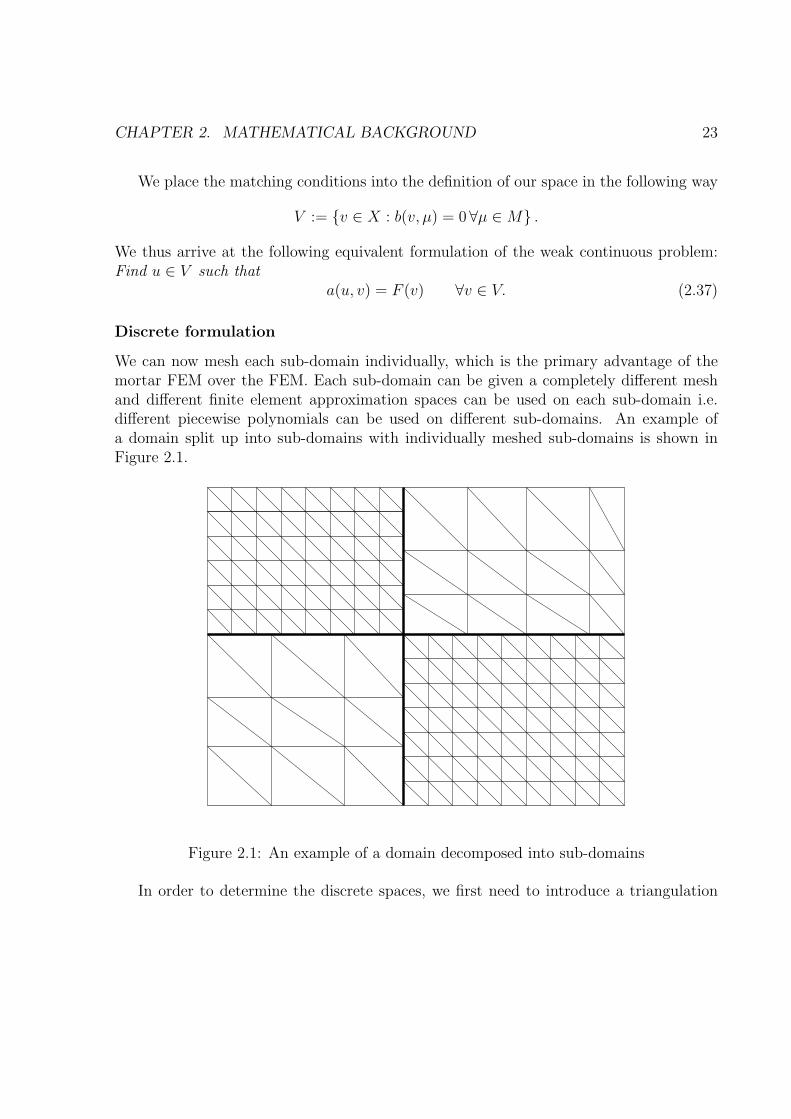
We can now mesh each sub-domain individually, which is the primary advantage of themortar FEM over the FEM. Each sub-domain can be given a completely different meshand different finite element approximation spaces can be used on each sub-domain i.e.different piecewise polynomials can be used on different sub-domains. An example ofa domain split up into sub-domains with individually meshed sub-domains is shown inFigure 2.1.
Figure 2.1: An example of a domain decomposed into sub-domains
In order to determine the discrete spaces, we first need to introduce a triangulation
CHAPTER 2. MATHEMATICAL BACKGROUND 24
Thiof each sub-domain Ωi, 1 ≤ i ≤ N , so that:
Ωi =⋃
κ∈Thi
κ,
where κ represents an element of the triangulation. For simplicity we may assume thatthe elements are triangles, although the results hold for other types of elements. Let usnow define the finite dimensional space:
Xh,i := vh,i ∈ C(Ωi), ∀κ ∈ Thi, vh,i ∈ P r(κ), vh,i|∂Ω∩∂Ωi
= 0.
We now consider the product space:
Xh :=N∏
i=1
Xh,i Xh ⊂ X.
We now consider the restriction of the triangulation Thiover Γij, 1 ≤ i ≤ N , j ∈ i,
with vertices ν1,ij and ν2,ij, results in a regular triangulation denoted by tij. Note that ingeneral tij differs from tji. The trace space of functions from Xh,i for the interface Γij isgiven by:
Wh,ij := χh,ij ∈ C(Γij), ∀t ∈ tij, χh,ij|t ∈ P r(t).
The local approximation of the Lagrange multipliers is taken locally in (a subspace ofWh,ij of co-dimension two)
Mh,ij := ψh,ij ∈ Wh,ij, ∀t ∈ tij, ψh,ij|t ∈ P r−1(t) if ν1,ij or ν2,ij ∈ t,
and we define the global discrete Lagrangian multiplier space to be:
Mh :=N∏
i=1
∏
j∈i
Mh,ij Mh ⊂M.
We thus have the following discrete mixed formulation. Find (uh, λh) ∈ Xh ×Mh suchthat
a(uh, vh) + b(vh, λh) = F (v) ∀vh ∈ Xh
b(uh, µh) = 0 ∀µh ∈Mh. (2.38)
The finite element functions that satisfy mortaring conditions form the space Vh ⊂ Xh
Vh := vh ∈ Xh : b(vh, µh) = 0 ∀µh ∈Mh . (2.39)
This leads to the alternative discrete formulation: Find uh ∈ Vh such that
a(uh, vh) = 〈f, vh〉Ω ∀vh ∈ Vh. (2.40)
CHAPTER 2. MATHEMATICAL BACKGROUND 25
Existence, uniqueness and error estimate
We shall now consider what is necessary for the existence and uniqueness of the solutionto the mortar FEM, and what is required to produce an error estimate. The followingensure the stability of the discrete formulation. Firstly we need the continuity of thebilinear forms a(., .) and b(., .) defined in (2.34) and (2.35) respectively with respect tothe appropriate norms:
|a(uh, vh)| ≤ c‖uh‖X‖vh‖X , ∀uh, vh ∈ Xh,
and|b(vh, µh)| ≤ c‖vh‖X‖µh‖M ∀uh ∈ Xh, ∀µh ∈Mh.
Next we require the ellipticity of a(., .) on the space Vh (defined in (2.39)) for the followingbound
a(vh, vh) ≥ α‖vh‖2X .
Now we need that the bilinear form b(·, ·) satisfies the the (discrete) LBB-condition(also known as the inf-sup condition)
infµh∈Mh
supvh∈Xh
b(vh, µh)
‖vh‖X‖µh‖M≥ β.
The existence and uniqueness of the solution (uh, µh) ∈ Xh×Mh follows from the Babuska-Brezzi theory (See Theorem 2.9). This requires that the bilinear form a(·, ·) is continuouson Xh and Vh-elliptic. It also requires that the bilinear form b(·, ·) satisfies a discreteinf-sup condition and is continuous on Xh ×Mh.
These results lead to the following error estimate, from the Strang-type estimate (The-orem 2.6).
Lemma 2.12. [3, Lemma 2.4] The discrete solution uh of (2.38) (or equivalently (2.40))and the exact solution u of (2.33) (or equivalently (2.37)) satisfy (where µ = ∂u
∂n)
‖u− uh‖X ≤ c
(infvh∈Vh
‖u− vh‖X + supvh∈Vh
b(vh, µ)
‖vh‖X
)
The first term on the right hand side is the approximation error; the second is theconsistency error. The consistency error results from the non-conformity of the method.Bounding the consistency error is relatively straightforward by the continuity of b(·, ·),however estimating the approximation error is not. The main difficulty involved is thatwe are taking the infimum over the constrained space Vh but we are approximating byfunctions in the unconstrained space Xh. This means that we need to construct a function
CHAPTER 2. MATHEMATICAL BACKGROUND 26
vh such that it satisfies the mortaring conditions if we wish to apply standard approxi-mation theory. This process involves the use of interpolation operators (and projectionoperators) and as such requires the assumption that the solution to the problem has atleast H1(Ωi) regularity. These projection and extension operators allow us to bound theapproximation error, see [6, Lemma 4.3 and Theorem 4.4].
We define the following mortar projection operator:
πij : H1/2(Γij) → Wh,ij ∩ H1/2(Γij)
as follows: ∀ψ ∈Mh,ij ∫
Γij
(χ− πijχ)ψ ds = 0.
Note that the function πijχ ∈ H1/2(Γij) is equivalent to the fact that it is vanishing atthe extreme points points of Γij. This projection operators projects functions from themortar side onto the Lagrangian multiplier (or non-mortar) side. We require the followingproperty of this projection operator.
Lemma 2.13. [3, Lemma 2.2] The projector πij is continuous: ∀χ ∈ H1/2(Γij),
‖πijχ‖H1/2(Γij)≤ C‖χ‖H1/2(Γij)
.
We next need the existence and stability of an extension operator for the traces of ourdiscrete functions from the boundary of a sub-domain over the whole sub-domain.
Lemma 2.14. [3, Lemma 2.3] There exists an extension operator
Ei : C(∂Ωi) ∩∏
j∈i
Wh,ij → Xh,i,
satisfying the stability‖Eiχ‖H1(Ωi) ≤ C‖χ‖H1/2(∂Ωi),
where C is a constant independent of hi.
We now arrive at the main error estimate.
Lemma 2.15. [3, Lemma 2.5] Assume the exact solution u of problem (2.33) (or equiv-alently (2.37)) is in H1
0 (Ω) is so that for any i, 1 ≤ i ≤ N , ui = u|Ωi∈ Hλi+1(Ωi),
0 ≤ λi ≤ r and for the discrete solution uh of (2.38) (or equivalently (2.40)) Then wehave
‖u− uh‖X ≤ CN∑
i=1
hλii ‖u‖
2Hλi+1(Ωi)
where hi is the maximum mesh size on Ωi.
CHAPTER 2. MATHEMATICAL BACKGROUND 27
Finally we note that in [3] the analysis does not stop at this point. An error estimate onthe Lagrange multiplier is also examined and the results are extended to the geometricalnonconforming case. However as this is only a brief outline we shall not proceed anyfurther.
When translating from the finite element to the boundary element situation there areseveral key issues that are going to have to be dealt with. Firstly we require a suitableintegration by parts formula which can be used to provide the boundary integral requiredfor the matching condition and the Lagrangian multipliers. A key issue here is the lack ofa suitable trace theorem for the restriction of functions to the boundary in the boundaryelement situation. Once an integration by parts formula has been derived we can thendefine the required bilinear forms. The appropriate properties of these bilinear forms mustthen be shown in order to use the theory already described. We shall also need to definesuitable extension and projection operators for our functions in order to get an errorestimate. Another issue to be overcome is that in general the solution to the BEM hasless regularity than that of the FEM, this will have an implication when examining theerror estimate of the scheme.
2.3 Technical Details
In this section we shall present some technical details on surface differential operators,transformation to a reference sub-domain and some other results. The surface differentialoperators are required for the integration by parts formula which will be used to provideus with the required interface matching conditions. The transformation to a referencesub-domain is included as it shows the dependence on the size of the sub-domain of ourresults. Other results that are used in later chapters are also included here in one commonplace for ease of reference.
2.3.1 Surface Differential Operators
We shall first define and discuss some surface differential operators which are requiredto generate an integration by parts formula for the hypersingular integral equation. Werecall that for simplicity we let Γ be the plane open surface (0, 1) × (0, 1) × 0, and weidentify it with the square (0, 1)2 ⊂ IR2.
We associate with any function ϕ on a generic surface piece S ⊂ Γ, a function ϕdefined in S × (−1, 1) by ϕ(x1, x2, x3) = ϕ(x1, x2). We shall also denote by n the unitnormal on S, e.g. n = (0, 0, 1)T . Then we define on S for a smooth function ϕ
gradS ϕ := (grad ϕ)|S, curlS ϕ := gradS ϕ× n.
CHAPTER 2. MATHEMATICAL BACKGROUND 28
Accordingly, we define for any sufficiently smooth tangential vector field ϕ on S
curlSϕ := n · (curl ϕ)|S.
Here, ϕ is defined component-wise. The definitions of gradS, curlS and curlS are ap-propriate for a non-flat smooth surface (using a coordinate direction normal to S insteadof x3 to define the extensions ϕ and ϕ) whereas, in our case of the flat surface S, theyobviously reduce to
gradS ϕ =(∂x1ϕ, ∂x2ϕ, 0
), curlS ϕ =
(∂x2ϕ,−∂x1ϕ, 0
),
curlS(ϕ1, ϕ2, 0) = ∂x1ϕ2 − ∂x2ϕ1.
In the following we extend the open surface S to a closed surface S. To distinguishbetween operators on different surfaces we add the notation of the corresponding surfaceas an index to the operator. We note that the following results also hold true on polyhedralsurfaces. In such cases, surface differential operators and corresponding trace spaces needto be dealt with as in [15].
In the following, S always denotes a closed, smooth surface extending the open surfaceS. Following [16], curlS can be extended to a continuous linear mapping from H1/2(S)
onto H−1/2t (S) where H
−1/2t (S) is the closure in (H−1/2(S))3 of
L2t (S) := ψ ∈
(L2(S)
)3; ψ · n = 0.
(Accordingly we will use the space L2t (S) below.) We use this extension to H1/2(S) to
define curlS on H1/2(S): Here we have that
curlS :
H1/2(S) → H
−1/2t (S) := ϕ ∈
(H−1/2(S)
)3; ϕ · n = 0
v 7→(curlS v
)|S
(2.41)
where v ∈ H1/2(S) is an extension of v. The well-posedness of this definition will be
proved in Lemma 2.16 below. To be precise, the definition of H−1/2t (S) in (2.41) is to be
understood as the trace of H−1/2t (S) onto S.
Lemma 2.16. ([25, Lemma 2.1]) The operator curlS : H1/2(S) →H−1/2t (S) defined by
(2.41) is continuous.
Proof. The continuity of curlS holds by the existence of an extension operator H1/2(S) →
H1/2(S), the continuity of curlS : H1/2(S) → H−1/2t (S) (see [16]) and the continuity of
the restriction H−1/2t (S) →H
−1/2t (S). The definition of curlS on H1/2(S) is independent
CHAPTER 2. MATHEMATICAL BACKGROUND 29
of the particular extension since, for given ϕ ∈ H1/2(S) and two extensions ϕ1, ϕ2 ∈H1/2(S), there holds (with ψ0 denoting the extension by zero onto S of ψ defined on S)
〈curlS(ϕ1 − ϕ2),ψ0〉S = 〈ϕ1 − ϕ2, curlSψ
0〉S = 〈ϕ1 − ϕ2, curlSψ〉S = 0 ∀ψ ∈ C∞0,t(S)
whereC∞
0,t(S) := ψ ∈(C∞
0 (S))3
; ψ · n = 0
is dense in the dual space (H−1/2t (S))′ = H
1/2
t (S).
Lemma 2.17. ([25, Lemma 2.2]) The restriction curlS |H1/2(S) is continuous as a mapping
H1/2(S) → H−1/2
t (S) where
H−1/2
t (S) := ψ ∈(H−1/2(S)
)3; ψ · n = 0.
Proof. We introduce the space
H1/2t (S) := ψ ∈
(H1/2(S)
)3; ψ · n = 0
and for a function ψ on S let ψ0 denote its extension onto S by 0. For ϕ ∈ C∞0 (S)
there holds(curlS ϕ
)0= curlS ϕ
0. Therefore, using the continuity of curlS : H1/2(S) →
H−1/2t (S), we obtain
‖ curlS ϕ‖H−1/2t (S)
= sup06=ψ∈H
1/2t (S)
〈curlS ϕ,ψ〉S‖ψ‖
H1/2t (S)
≃ sup06=ψ∈H
1/2t (S)
〈(curlS ϕ
)0, ψ〉S
‖ψ‖H
1/2t (S)
= ‖ curlS ϕ0‖H
−1/2t (S)
≤ C ‖ϕ0‖H1/2(S) ≃ ‖ϕ‖H1/2(S) ∀ϕ ∈ C∞0 (S).
Here ≃ denotes the equivalence of norms. The assertion follows by the density of C∞0 (S)
in H1/2(S).
Lemma 2.18. ([28, Lemma 3.4]) The operator curlS : H12+s(S) → H
− 12+s
t (S) is contin-uous for s ∈ [0, 1/2].
Proof. By Lemma 2.16 curlS : H12 (S) → H
− 12
t (S) is continuous, and curlS : H1(S) →L2t (S) = H0
t (S) is continuous as well (see e.g. [15, Proposition 3.3]). The result followsby interpolation.
Lemma 2.19. ([25, Lemma 4.1]) There exists a positive constant C such that
|ϕ|H1/2(S) ≤ C ‖ curlS ϕ‖H−1/2t (S)
∀ϕ ∈ H1/2(S).
CHAPTER 2. MATHEMATICAL BACKGROUND 30
Proof. By Lemma 2.16, curlS : H1/2(S) → H−1/2t (S) is continuous. We also have that
the range of curlS is closed in H−1/2t (S). This follows from the closedness of the range
of curlS : H1/2(S) →H−1/2t (S) (see [16]) where S is, as before, a smooth, closed surface
containing S. Since the range of curlS : H1/2(S) → H−1/2t (S) is the restriction onto
S of the range of curlS : H1/2(S) → H−1/2t (S), the closedness of the range of curlS
follows, see e.g. [41, pp. 76f.]. Next we see that the kernel of curlS in H1/2(S) consistsof constant functions. This follows by noting that any ϕ ∈ H1/2(S) with curlS ϕ = 0satisfies ϕ ∈ H1(S) such that curlS ϕ is defined in the usual weak sense. The kernel ofcurlS |H1(S) is given by the constant functions. Therefore, an application of the closedgraph theorem yields the estimate
infc∈IR
‖ϕ− c‖H1/2(S) ≤ C ‖ curlS ϕ‖H−1/2t (S)
∀ϕ ∈ H1/2(S),
and the assertion follows by the Poincare-Friedrichs inequality.
2.3.2 Integration By Parts Formula
We now turn our attention to an integration-by-parts formula. We require an integrationby parts formula to create the boundary terms which shall be used as our integral match-ing condition in the mortar BEM. Before presenting an integration by parts formula weshall reexpress the hypersingular operator in terms of surface differential operators. Anintegration by parts formula may then be applied to this alternative formulation.
In the following we need the single layer potential operator V . It is defined by
Vϕ(x) :=1
4π
∫
Γ
ϕ(y)
|x− y|dSy, ϕ ∈ (H−1/2(Γ))3, x ∈ Γ. (2.42)
It is well-known, and widely used in the boundary element literature, that the singlelayer potential operator V can be used to represent the hypersingular operator W , andthat their bilinear forms relate like an integration-by-parts formula. This goes back toNedelec [43] who studied the case of a closed smooth surface. Other equations than theLaplace equation have been examined to show how their representations by hypersingularintegral operators can be reexpressed in terms of weakly singular operators, see [40, 43] forHelmholtz and Maxwell equations in three dimensions and [27, 43] for the Lame systemin three dimensions. All the authors mentioned above considered closed smooth systems.Since we did not find a reference for open surfaces we recall this situation in the nextlemma.
Lemma 2.20. (e.g. [25, Lemma 2.3]) There holds
W = curlΓ V curlΓ in L(H1/2(Γ), H−1/2(Γ)). (2.43)
CHAPTER 2. MATHEMATICAL BACKGROUND 31
Moreover〈Wφ,ψ〉Γ = 〈V curlΓ ψ, curlΓ φ〉Γ ∀φ, ψ ∈ H1/2(Γ). (2.44)
Proof. Using the surface differential operators introduced before, there holds in the dis-tributional sense Wφ = curlΓ V curlΓ φ, see [40, 43]. This formula extends from C∞
0 (Γ)
to φ ∈ H1/2(Γ) since curlΓ : H1/2(Γ) → H−1/2
t (Γ) by Lemma 2.17, V : H−1/2
t (Γ) →
H1/2t (Γ) by [19], and curlΓ : H
1/2t (Γ) → H−1/2(Γ) since it is the adjoint operator of
curlΓ, cf. [15]. The relation (2.44) follows by integration by parts.
Towards integration by parts
We now present an integration by parts formula.
Lemma 2.21. (See e.g. [51, Lemma 6.16]) For a smooth scalar function v and a smoothtangential vector field ϕ, integration by parts gives
〈curlΓ v,ϕ〉Γ = −〈v, curlΓϕ〉Γ + 〈v,ϕ · t〉γ. (2.45)
Proof. Using the product rule
∇× [vϕ] = ∇v ×ϕ+ v[∇×ϕ]
we obtain ∫
Γ
curlΓ v ·ϕ =
∫
Γ
[∇v × n] ·ϕ
= −
∫
Γ
[n×∇v] ·ϕ
= −
∫
Γ
[∇v ×ϕ] · n
= −
∫
Γ
[∇× [vϕ] − v[∇×ϕ]] · n
=
∫
Γ
v curlΓϕ−
∫
γ
vϕt
by applying the integral theorem of Stokes.
For a smooth scalar function v and a smooth tangential vector field ϕ, integration byparts gives
〈curlΓ v,ϕ〉Γ = 〈v, curlΓϕ〉Γ − 〈v,ϕ · t〉γ. (2.46)
Here, t is the unit tangential vector on γ (oriented mathematically positive when identi-fying Γ with (0, 1)2). We note that if we choose functions v such that they vanish at theboundary e.g. v ∈ H1/2(Γ) then the integral over γ disappears and we are left with
〈curlΓ v,ϕ〉Γ = 〈v, curlΓϕ〉Γ.
CHAPTER 2. MATHEMATICAL BACKGROUND 32
The Trace Theorem
We now present the following result on the trace operator to show why the integration byparts formula (2.46) does not hold for continuous discrete functions in H1/2(Γ) which donot vanish on γ (the boundary of Γ).
Lemma 2.22. ([25, Lemma 4.3]) There exists C > 0 such that, for any ǫ ∈ (0, 1/2),there holds
‖v‖L2(γ) ≤C
ǫ1/2‖v‖H1/2+ǫ(Γ) ∀v ∈ H1/2+ǫ(Γ).
Proof. The trace theorem is usually proved by applying local mappings onto the half-spacecase where the Fourier transformation is used. This yields the estimate
‖v‖2L2(γ) ≤ CMs ‖v‖
2Hs(Γ) ∀v ∈ Hs(Γ), 1/2 < s ≤ 1,
with C depending only on Γ and with
Ms =
∫
IR(1 + t2)−s dt,
see, e.g., [41, Lemma 3.35, Theorem 3.37]. We note that the norms in Hs(Γ) defined by(2.1) and by Fourier transformation are uniformly equivalent for s ∈ J and any closedinterval J ⊂ (0, 1) (see the proof of Lemma 4.1 in [24]). Therefore, the statement isproved for small ǫ > 0 (bounded away from 1/2) by noting that M1/2+ǫ = O(ǫ−1). Forlarger ǫ the result follows by the continuous injection of higher order Sobolev spaces inlower order spaces.
Specifically Lemma 2.22 is defined for ǫ on the (open) interval (0, 1/2). Thus for asimple translation from the finite element to the boundary element situation we wouldreplace v ∈ H1/2(Γ) by v ∈ H1/2(Γ). If we apply the integration by parts formula (2.46)to a function in H1/2(Γ) we see that the boundary term requires the restriction of thisfunction to the boundary and Lemma 2.22 shows that this is not possible.
2.3.3 Transformation To a Reference Sub-Domain
The following two Lemmas describe the behaviour of Sobolev norms on regions of differentsizes.
Lemma 2.23. [29, Lemma 2] Let In = (0, 1)n, Inh = (0, h)n and let
T nh : Inh → In, n = 1, 2, 3,
CHAPTER 2. MATHEMATICAL BACKGROUND 33
be an affine transformation. For functions u, u such that u = u T nh on Inh there holdsfor n = 1, 2, 3
‖u‖2Hs(In
h )≃ hn−2s‖u‖2
Hs(In)(0 ≤ s ≤ 1),
and‖u‖2
Hs(Inh ) ≃ hn−2s‖u‖2
Hs(In) (−1 ≤ s ≤ 0).
Lemma 2.24. [29, Lemma 3] We use the same notation as in Lemma 2.23. For afunction u with integral mean zero on Inh there holds for n = 1, 2, 3
‖u‖2Hs(In
h ) ≃ hn−2s‖u‖2Hs(In) (0 ≤ s ≤ 1),
and‖u‖2
Hs(Inh )
≃ hn−2s‖u‖2Hs(In)
(−1 ≤ s ≤ 0),
provided one of the respective norms is finite.
For a given S ⊂ Γ we denote by TS an affine bijective transformation from the referencedomain S onto S. The reference domain in the case of a triangular mesh of the (sub-)domain S is S = (x1, x2); 0 ≤ x1, x2 ≤ 1, x1 + x2 ≤ 1 and in the case of a rectangularmesh is S = (x1, x2); 0 ≤ x1, x2 ≤ 1. Also, given v : S → IR we write v := v TS. We
shall also use the notation curlS := curlS.For S ⊂ Γ of (maximum) diameter DS with (maximum) mesh size hS, we have the
following equivalence of semi-norms when transforming to (and from) a reference domain
|v|2Hr(S)∼= D2−2r
S |v|2Hr(S)
0 ≤ r ≤ 1. (2.47)
We also note that the mesh size on the reference domain is now
hSDS
.
This is important as in later chapters we are going to transform to a reference sub-domainand then apply results which have a dependence upon the mesh size on the sub-domain.
In the following we shall not be using functions with integral mean zero, so we cannotapply the results of Lemma 2.24. However, we shall need to know the effect of the diameterof the domain when transforming the norms used in Lemma 2.24.
Lemma 2.25. For 0 ≤ r ≤ 1 and 0 < DS ≤ 1, we have
‖v‖2Hr(S) & D2
S‖v‖2Hr(S)
and ‖v‖2Hr(S)
. D−2S ‖v‖2
Hr(S) (2.48)
and‖v‖2
Hr(S) . D2−2rS ‖v‖2
Hr(S)and ‖v‖2
Hr(S)& D2r−2
S ‖v‖2Hr(S). (2.49)
CHAPTER 2. MATHEMATICAL BACKGROUND 34
Proof. For 0 ≤ r ≤ 1 we have by (2.47)
‖v‖2Hr(S) = ‖v‖2
L2(S) + |v|2Hr(S)
∼= D2S‖v‖
2L2(S)
+D2−2rS |v|2
Hr(S).
Now noting that for 0 < DS ≤ 1 we have D2S ≤ D2−2r
S we get (2.48) and (2.49).
Similarly for the one dimensional situation we have the interval κ of length Kκ istransformed to the interval κ of unit length.We now have
|v|2Hr(κ)∼= K1−2r
κ |v|2Hr(κ) 0 ≤ r ≤ 1. (2.50)
Lemma 2.26. For 0 ≤ r ≤ 1/2 and 0 < Kκ ≤ 1, we have
‖v‖2Hr(κ) & Kκ‖v‖
2Hr(κ) and ‖v‖2
Hr(κ) . K−1κ ‖v‖2
Hr(κ) (2.51)
and‖v‖2
Hr(κ) . K1−2rκ ‖v‖2
Hr(κ) and ‖v‖2Hr(κ) & K2r−1
κ ‖v‖2Hr(κ). (2.52)
Proof. For 0 ≤ r ≤ 1/2 we have by (2.50)
‖v‖2Hr(κ) = ‖v‖2
L2(κ) + |v|2Hr(κ)
∼= Kκ‖v‖2L2(κ) +K1−2r
κ |v|2Hr(κ).
Now noting that for 0 < Kκ ≤ 1 we have Kκ ≤ K1−2rκ we get (2.51) and (2.52).
We next examine the effect of our surface differential operator curlS on the scalingproperties of certain norms.
Lemma 2.27. For 0 ≤ r ≤ 1 we have for 0 < DS ≤ 1 we have
‖ curlS v‖2H−r
t (S)∼= D2r
S ‖ curlS v‖2H−r
t (S).
Proof. For 0 ≤ r ≤ 1 and 0 < DS ≤ 1 we have, noting that curlS scales like D−1S (on a
two dimensional domain)
‖ curlS v‖2H−r
t (S)∼= D2+2r
S D−2S ‖ curlS v‖
2H−r
t (S).
The stated result now follows immediately.
CHAPTER 2. MATHEMATICAL BACKGROUND 35
Lemma 2.28. For 0 ≤ r ≤ 1 we have for 0 < DS ≤ 1 we have
‖ curlS v‖2
H−rt (S)
& D2rS ‖ curlS v‖
2
H−rt (S)
. (2.53)
and‖ curlS v‖
2H−r
t (S). ‖ curlS v‖
2H−r
t (S). (2.54)
Proof. For 0 ≤ r ≤ 1 and 0 < DS ≤ 1 we have
‖ curlS v‖H−rt (S)
= supϕ∈Hr
t (S)
〈ϕ, curlS v〉S‖ϕ‖Hr
t (S)
= supϕ∈Hr(S)
〈ϕ, curlS v〉S(‖ϕ‖2
L2t (S)
+ |ϕ|2Hr
t (S)
)1/2
∼= supϕ∈Hr
t (S)
DS〈ϕ, curlS v〉S(D2S‖ϕ‖
2L2
t (S)+D2−2r
S |ϕ|2Hr
t (S)
)1/2
Using this we can now get the following bounds:
‖ curlS v‖H−rt (S)
& supϕ∈Hr
t (S)
DS〈ϕ, curlS v〉SD1−rS ‖ϕ‖
Hrt (S)
∼= DrS‖ curlS v‖H−r
t (S),
which gives us (2.53). For the other bound
‖ curlS v‖H−rt (S) . sup
ϕ∈Hrt (S)
DS〈ϕ, curlS v〉SDS‖ϕ‖Hr
t (S)
∼= ‖ curlS v‖H−rt (S),
which gives us (2.54).
2.3.4 Other Required Results
The following is a result that allows us to bound the tilde norm of a function by thenon-tilde norm.
Lemma 2.29. [29, Lemma 5] Let R ⊂ IR2 be a Lipschitz domain. There exists C > 0such that for any s ∈ (−1/2, 1/2) and any v ∈ Hs(R) there holds
‖v‖Hs(R) ≤C
1/2 − |s|‖v‖Hs(R).

CHAPTER 2. MATHEMATICAL BACKGROUND 36
Lemma 2.30. ([28, Lemma 3.2]) Let v ∈ H−1/2(R), R ⊂ IR2 a Lipschitz domain, be apiecewise linear function defined on a quasi-uniform mesh on R with mesh size h < 1.There exists a constant C > 0 which is independent of h (but may depend on the diameterof R) such that there holds
‖v‖H−1/2(R) ≤ C| log(h)|‖v‖H−1/2(R).
Proof. By [29, Lemma 6] there holds for a piecewise polynomial of degree p the estimate
‖v‖H−1/2(R) ≤ C log(p+ 1
h)‖v‖H−1/2(R) p ≥ 0, h < 1.
Fixing p gives the claimed bound. The proof of [29, Lemma 6] gives full details forrectangular meshes. For triangular meshes the proof applies as well by making use ofSchmidt’s inequality for triangles, cf. [21, Lemma 5.1]. Nevertheless, we are consideringonly polynomials of low degrees where Schmidt’s inequality is not needed.
The next Lemma shows the relationships between Sobolev norms over the whole do-main and the respective Sobolev norms over sub-domains.
Lemma 2.31. [29, Lemma 1] Let Γ be a Lipschitz domain in IR2 and let Γj; j = 1, . . . , Jbe a decomposition of Γ into J Lipschitz domains, i.e.
J⋃
j=1
Γj = Γ and Γi ∩ Γj = ∅ if i 6= j.
Moreover we assume that
1. for each of the domain Γj, j = 1, . . . , J a finite number (being independent of j andJ) of Lipschitz mappings can be used to describe its boundary and that
2. the Lipschitz constants of all the boundary mappings are uniformly bounded.
Then for s ∈ [−1, 1] and u ∈ Hs(Γ) with uj := u|Γj∈ Hs(Γj), j = 1, . . . , J , there exists a
constant c > 0 which is independent of s, u, and J such that
‖u‖2Hs(Γ)
≤ c
J∑
j=1
‖uj‖2Hs(Γj)
.
Further, for arbitrary u ∈ Hs(Γ),
J∑
j=1
‖uj‖2Hs(Γj)
≤ c‖u‖2Hs(Γ)
for a constant c that is independent of s, u, and J .
CHAPTER 2. MATHEMATICAL BACKGROUND 37
The next lemma deals with the inverse property of piecewise polynomials.
Lemma 2.32. [29, Lemma 4] Let Γ be a polygonal domain and let Γj : j = 1, . . . , J bea rectangular mesh on Γ which is assumed to be quasi-uniform, the lengths of the elementsbeing proportional to h. Further let v be a piecewise polynomial of degree p, i.e. v|Γj
is a
polynomial of degree p for j = 1, . . . , J . If v ∈ Hr(Γ) for a real number r ≤ 1, then fors ≤ r there holds
‖v‖Hr(Γ) ≤ chs−rp2(r−s)‖v‖Hs(Γ).
Accordingly, for v ∈ Hr(Γ), there holds
‖v‖Hr(Γ) ≤ chs−rp2(r−s)‖v‖Hs(Γ).
Here, c is a constant that is independent of h and p and, for given r∗, s∗ (s∗ ≤ r∗), isalso independent of r and s for s∗ ≤ s ≤ r ≤ r∗.
Chapter 3
The BEM with LagrangianMultiplier
In this chapter we present the formulation of the BEM with Lagrangian multiplier. Weintend to present the BEM analogue to the method discussed in Section 2.2.3. We shallconsider the model situation of the hypersingular operator for the Laplace operator ona plane open surface. A discrete variational formulation shall be presented and anal-ysed. Particular attention shall be paid to the continuity and ellipticity of appearingbilinear forms. An error estimate shall be obtained and compared to that of the stan-dard (conforming) BEM formulation. Numerical results which underline the theory shallbe presented later in Chapter 5. This chapter, along with parts of Section 2.3.1 andChapter 5 have been published in [25].
3.1 Towards a Discrete Formulation
3.1.1 Introduction and Model Problem
Model problem
Now we introduce the model problem. For simplicity let Γ be the plane open surface(0, 1)× (0, 1)×0. We will identify it with the square (0, 1)2 ⊂ IR2. Our model problemis: For given f ∈ H−1/2(Γ) find φ ∈ H1/2(Γ) such that
Wφ(x) = f(x), x ∈ Γ. (3.1)
See (2.7) for the definition of W and recall that W : H1/2(Γ) → H−1/2(Γ) (see [19]).Nevertheless, we require f to be slightly more regular than in the standard boundary ele-ment formulation (see (2.7)). We require f ∈ H−1/2(Γ) ⊂ H−1/2(Γ). This will be needed
38
CHAPTER 3. THE BEM WITH LAGRANGIAN MULTIPLIER 39
below when testing f with elements of H1/2(Γ), rather than in the standard formulation(see Section 2.1.1) where we tested with elements of H1/2(Γ). This requirement of extraregularity when compared to the standard formulation (2.7), which required f ∈ H−1/2(Γ)is not a problem, in particular we note that H1/2(Γ) ⊂ H1/2(Γ).
The variational formulation of (3.1) is: Find φ ∈ H1/2(Γ) such that
〈Wφ,ψ〉Γ = 〈f, ψ〉Γ ∀ψ ∈ H1/2(Γ). (3.2)
We recall a standard BEM (see (2.8)) for the approximate solution of (3.2) is to selecta piecewise polynomial subspace Xh ⊂ H1/2(Γ) and to define an approximant φh ∈ Xh by
〈Wφh, ψ〉Γ = 〈f, ψ〉Γ ∀ψ ∈ Xh.
The conformity condition Xh ⊂ H1/2(Γ) requires that any v ∈ Xh vanishes on the bound-ary γ of Γ. Instead of this formulation we shall examine a non-conforming discretisationof (3.2) by using subspaces Xh whose elements do not necessarily vanish on γ (see Sec-tion 2.2.2). Our subspaces will satisfy Xh ⊂ H1/2(Γ) where Xh 6⊂ H1/2(Γ). We thushave a non-conforming discretisation since our discrete space is not a subset of the con-tinuous space. The boundary condition is incorporated weakly by using a Lagrangianmultiplier. This means that we do not directly incorporate the boundary condition intothe definition of the space. Instead it is included through the inclusion of an additionalboundary integral. Note that the natural domain of definition of the hypersingular oper-ator W is H1/2(Γ) and not H1/2(Γ). This means that we cannot directly substitute ournon-conforming discrete space into the problem since the action of W on elements of thisspace is not well defined, unlike in the FEM situation (see Section 2.2.3). We thereforeneed to deal with boundary data for an appropriate definition of W and this requiresan integration-by-parts formula. We need a way to rewrite W so that it is well definedfor functions in our non-conforming discrete space and also supplies us with a suitableboundary term that can be used to define the Lagrangian multipliers.
First let us consider the situation of the conforming continuous formulation (3.2). Afterthat we will study a non-conforming discrete setting. There will be no non-conformingcontinuous formulation (i.e. a version of (3.2) with H1/2(Γ) replaced by H1/2(Γ)). Thisis due to the fact that integration by parts involves the trace operator which is not welldefined on H1/2(Γ) (see the Trace Theorem, Lemma 2.22). We shall use our integration byparts formula to introduce an appropriate boundary term which can be used to incorporatethe boundary condition in a weak sense (through a Lagrangian multiplier), and also toreduce the regularity requirements on our approximating functions relative to the standardBEM formulation (we replace H1/2(Γ) by H1/2(Γ)).
CHAPTER 3. THE BEM WITH LAGRANGIAN MULTIPLIER 40
Conforming continuous formulation
An immediate consequence of Lemma 2.20 is that an equivalent variational formulationof (3.1) is: Find φ ∈ H1/2(Γ) such that
〈V curlΓ φ, curlΓ ψ〉Γ = 〈f, ψ〉Γ ∀ψ ∈ H1/2(Γ). (3.3)
This weak formulation forms the starting point for the BEM with Lagrangian multiplier.For definitions of the surface differential operators and the weakly singular integral op-erator see Sections 2.3.1 and 2.3.2. This formulation is well known and widely used inthe field of boundary elements. This is because it is computationally easier to implementthe weakly singular integral operator than the hypersingular integral operator due to thenature of the appearing singularities.
Note that we will consider discrete subspaces of H1/2(Γ) where the hypersingularoperator W is not well defined (recall W is well defined for functions in H1/2(Γ)). Theformulation (3.3) does make sense for continuous discrete functions which do not vanish onγ (the boundary of Γ), whereas the formulation (3.2) does not. Nevertheless, for the erroranalysis of our scheme we must relate a discrete version of (3.3) with the original problem(3.1), i.e. with (3.2). This requires an integration-by-parts formula that corresponds to(2.44) but is valid for functions which do not vanish on γ.
3.1.2 Integration By Parts
Applying the integration by parts formula (2.46) to (2.43) we obtain, for sufficientlysmooth φ and ψ,
〈t · V curlΓ φ, ψ〉γ = 〈Wφ,ψ〉Γ − 〈V curlΓ φ, curlΓ ψ〉Γ. (3.4)
This formula does not extend to ψ ∈ H1/2(Γ) since the trace of such a ψ onto γ is not welldefined (by the Trace Theorem, Lemma 2.22). We now have an alternative formulationof W in terms of V and curlΓ that can be used to define a Lagrangian multiplier in thecase where we have non-conforming approximating functions that do not vanish at theboundary. We define the Lagrangian multiplier λ as
λ = t · V curlΓ φ.
The vanishing condition can now be incorporated using the boundary (of the boundary)integral (the integral over γ), however this term also requires the restriction of the functionψ to the boundary to be well defined. This is not the case for ψ ∈ H1/2(Γ) as describedearlier, so we will have to assume slightly more regularity for our approximating functionsin order for this term to be well defined and thus allow us to include the vanishing
CHAPTER 3. THE BEM WITH LAGRANGIAN MULTIPLIER 41
condition in a weak sense. However, we do not require any extra regularity on φ sincethere holds the following lemma which guarantees sufficient regularity of our Lagrangianmultiplier term.
Lemma 3.1. ([25, Lemma 4.2]) For φ ∈ H1/2(Γ) with Wφ = f ∈ H−1/2(Γ), (3.4) definest · V curlΓ φ ∈ H−1/2(γ).
Proof. Extending ψ ∈ H1/2(γ) to an element of H1(Γ) (using the same name) there holds
|〈t · V curlΓ φ, ψ〉γ| = |〈f, ψ〉Γ − 〈V curlΓ φ, curlΓ ψ〉Γ|
≤ ‖f‖H−1/2(Γ)‖ψ‖H1/2(Γ) + ‖V curlΓ φ‖L2t (Γ)‖ curlΓ ψ‖L2
t (Γ)
≤ (‖f‖H−1/2(Γ) + ‖V curlΓ φ‖H1/2t (Γ)
)‖ψ‖H1(Γ)
withL2t (Γ) := ψ ∈
(L2(Γ)
)3; ψ · n = 0.
The result follows by using the continuity of curlΓ : H1/2(Γ) → H−1/2
t (Γ)
(see Lemma 2.17) and V : H−1/2
t (Γ) → H1/2t (Γ) (cf. the proof of Lemma 2.20), and by
the continuity of the extension of ψ ∈ H1/2(γ) to ψ ∈ H1(Γ).
Remark 3.2. Lemma 3.1 easily generalises to t · V curlΓ φ ∈ Hs(γ) with s ∈ (−1, 0)(requiring f ∈ Hs−1/2(Γ) in general) but breaks down for s = 0. The problem in the case
s = 0 is that the relevant required mapping property V : H−1/2
t (Γ) → H1/2
t (Γ) does nothold. But note that there is an extension operator L2(γ) → H1/2(Γ) (see [42, Lemma2.3]).
Note also that given f ∈ Hs(Γ), there exist non-unique extensions to f ∈ Hs(Γ) fors ∈ (−3/2, 1/2). Such an extension need not exist for s = −1/2 but is unique if it doesexist, see [42, Lemma 5].
In the proof of our main result for this chapter (Theorem 3.7) we will need (3.4)only for functions ψ ∈ H1/2(γ), and for uniqueness of f and t · V curlΓ φ we requiref ∈ H1/2(Γ).
3.1.3 Discrete Variational Formulation with Lagrangian Multi-plier
In this section we introduce a BEM formulation with Lagrangian multiplier. In orderto introduce the discrete scheme let us define a regular, quasi-uniform mesh Th of shaperegular elements T ∈ Th such that Γ = ∪T∈Th
T . As usual, h denotes the mesh size (beingproportional to the diameters of the elements). Throughout we assume that h < 1. This isno restriction of generality and is just needed to simplify the writing of logarithmic terms.
CHAPTER 3. THE BEM WITH LAGRANGIAN MULTIPLIER 42
Elements can be triangles or quadrilaterals. Using this mesh we define the boundaryelement space
Xh := φ ∈ C0(Γ); φ|T is a polynomial of degree one ∀T ∈ Th.
Note that Xh ⊂ H1/2(Γ), but Xh 6⊂ H1/2(Γ). While Xh ⊂ H1/2(Γ) it is important tonote that it is not equal to it. Our integration by parts formula is not well defined forfunctions in H1/2(Γ), however it is well defined for functions in Xh. This is why we haveno continuous formulation but do have a discrete formulation.
For the definition of a discrete Lagrangian multiplier space we introduce a quasi-uniform mesh Gk on γ = ∂Γ that consists of straight line pieces J ∈ Gk: γ = ∪J∈Gk
J .The parameter k refers to the mesh size of Gk (being proportional to the lengths of theelements). The discrete space for the Lagrangian multiplier is
Mk := q ∈ L2(γ); q|J is constant ∀J ∈ Gk.
We also define the bilinear forms
a(φ, ψ) := 〈V curlΓ φ, curlΓ ψ〉Γ,
b(φ, q) := 〈φ, q〉γ :=
∫
γ
φq ds,
the linear formF (φ) := 〈f, φ〉Γ,
and the spaceVh := φ ∈ Xh; b(φ, q) = 0 ∀q ∈Mk.
The boundary element scheme with Lagrangian multiplier for the approximate solutionof (3.3) then is: Find (φh, λk) ∈ Xh ×Mk such that
a(φh, ψ) + b(ψ, λk) = F (ψ) ∀ψ ∈ Xh,b(φh, q) = 0 ∀q ∈Mk.
(3.5)
This scheme is equivalent to
φh ∈ Vh : a(φh, ψ) = F (ψ) ∀ψ ∈ Vh.
Scheme (3.5) has the typical saddle point structure of a variational formulation withLagrangian multiplier. In the finite element case such a scheme is usually analysed by theBabuska-Brezzi theory (Section 2.2.4), see also [1]. Our situation, however, is not standardin the sense that there is no corresponding continuous saddle point formulation (whichis required in standard analysis). Also, we do not intend to derive an error estimate forthe Lagrangian multiplier since the corresponding continuous unknown is not well definedwhen φ ∈ H1/2(Γ) (it is t · V curlΓ φ with t being the unit tangential vector along γin mathematically positive sense, see (3.4)). Also the Lagrangian multiplier does notrepresent any physical property in our situation like it does in some mixed-formulations.
CHAPTER 3. THE BEM WITH LAGRANGIAN MULTIPLIER 43
3.2 Technical Results and Proof of the Main Result
Obviously, continuity and Vh-ellipticity of a(·, ·) are critical for the error analysis of (3.5).Lemma 3.3 below shows the continuity and then Lemma 3.5 proves that a(·, ·) is almostuniformly Vh-elliptic.
Continuity of a(·, ·)
Lemma 3.3. ([25, Lemma 4.4]) The bilinear form a(·, ·) is almost uniformly continuouson Xh. More precisely there holds the following upper bounds
a(v, w) . | log h|‖v‖H1/2(Γ)‖ curlΓw‖H−1/2t (Γ)
∀v, w ∈ Xh,
anda(v, w) . | log h|2‖v‖H1/2(Γ)‖w‖H1/2(Γ) ∀v, w ∈ Xh.
Proof. By the continuity of V : H−1/2
t (Γ) →H1/2t (Γ) there holds
a(v, w) . ‖ curlΓ v‖H−1/2t (Γ)
‖ curlΓw‖H−1/2t (Γ)
.
By Lemma 2.30 we have that for any piecewise polynomial on a quasi-uniform mesh
‖ curlΓ v‖H−1/2t (Γ)
. | log h|‖ curlΓ v‖H−1/2t (Γ)
∀v ∈ Vh. (3.6)
Now applying the continuity of curlΓ : H1/2(Γ) →H−1/2t (Γ) proves both assertions.
Ellipticity of a(·, ·)
The next result will be required to prove the ellipticity of the bilinear form a(·, ·).
Lemma 3.4. ([25, Lemma 4.5]) The exists C > 0 such that for any h ∈ (0, 1) and forsufficiently small k there holds
|v|H1/2(Γ) ≥ C| log h|−1/2‖v‖H1/2(Γ) ∀v ∈ Vh.
If k is proportional to a positive power of h then k satisfies the assumption if h is suffi-ciently small.
Proof. We decompose any v ∈ Vh into v = v0 + d with∫Γv0(x) dSx = 0 such that d =
|Γ|−1∫
Γv(x) dSx. In order to estimate d we note that there holds ‖d‖H−1(γ) = |d| ‖1‖H−1(γ),
that is
|d| = ‖1‖−1
H−1(γ)sup
q∈H1(γ)\0
〈d, q〉γ‖q‖H1(γ)
. (3.7)
CHAPTER 3. THE BEM WITH LAGRANGIAN MULTIPLIER 44
Since v ∈ Vh, i.e. b(v, qk) = 0 for any qk ∈Mk, we find
|〈d, q〉γ| = |〈v − v0, q〉γ| = |〈v, q − qk〉γ − 〈v0, q〉γ|
≤ ‖v‖L2(γ)‖q − qk‖L2(γ) + ‖v0‖L2(γ)‖q‖L2(γ) ∀qk ∈Mk.
We bound the L2(γ)-norms of v and v0 using Lemma 2.22 with a small ǫ > 0 and use theerror bound
infqk∈Mk
‖q − qk‖L2(γ) ≤ Ck‖q‖H1(γ).
The previous estimate then yields
|〈d, q〉γ| ≤C
ǫ1/2k‖v‖H1/2+ǫ(Γ)‖q‖H1(γ) +
C
ǫ1/2‖v0‖H1/2+ǫ(Γ)‖q‖H1(γ).
Applying the inverse property ‖v‖H1/2+ǫ(Γ) ≤ Ch−ǫ‖v‖H1/2(Γ) (see, e.g., Lemma 2.32)andselecting ǫ := 1/| log h| for h < 1, we conclude that there holds
|〈d, q〉γ| ≤ C| log h|1/2(k‖v‖H1/2(Γ) + ‖v0‖H1/2(Γ)
)‖q‖H1(γ).
Making use of (3.7) this yields
|d| ≤ C| log h|1/2(k‖v‖H1/2(Γ) + ‖v0‖H1/2(Γ)
). (3.8)
Therefore, using the triangle inequality, we estimate
‖v‖2H1/2(Γ) ≤ C(‖v0‖
2H1/2(Γ) + d2) ≤ C | log h|‖v0‖
2H1/2(Γ) + C | log h|k2‖v‖2
H1/2(Γ),
such that
(1 − C k2| log h|)‖v‖2H1/2(Γ) ≤ C | log h|‖v0‖
2H1/2(Γ)
= C | log h|(|v0|
2H1/2(Γ) + inf
c∈IR‖v − c‖2
L2(Γ)
)
= C | log h||v|2H1/2(Γ).
In the last step we made use of the Poincare-Friedrichs inequality. Selecting k small enoughsuch that 1 − C k2| log h| > 0 and dividing by 1 − C k2| log h| proves the lemma.
The next lemma states three variants of ellipticity for the bilinear form a(·, ·). Part(i) will be used to establish our computational error bound (5.1) needed for the nu-merical experiment. Part (ii) is essential for proving the Strang-type error estimate (seeLemma 2.6) of Theorem 3.6. Part (iii) proves the Vh-ellipticity with H1/2(Γ)-norm neededfor the Babuska-Brezzi theory (see Section 2.2.4). We note that part (iii) would be enoughto prove a Strang-type estimate and eventually an a priori error bound, but the ellipticityprovided by (ii) leads to a sharper bound.
CHAPTER 3. THE BEM WITH LAGRANGIAN MULTIPLIER 45
Lemma 3.5. ([25, Lemma 4.6]) (i) There holds
a(v, v) & |v|2H1/2(Γ) ∀v ∈ H1/2(Γ) ∪H1(Γ).
(ii) There holds for any h ∈ (0, 1) and sufficiently small k
a(v, v) & | log h|−1/2‖v‖H1/2(Γ)‖ curlΓ v‖H−1/2t (Γ)
∀v ∈ Vh.
If k is proportional to a positive power of h then k satisfies the assumption if h is suffi-ciently small.(iii) Under the conditions of part (ii) there holds
a(v, v) & | log h|−1‖v‖2H1/2(Γ) ∀v ∈ Vh.
Proof. We first note that a(v, v) is well defined for any v ∈ H1/2(Γ)∪H1(Γ). This follows
from the mapping properties of V and the continuities curlΓ : H1/2(Γ) → H−1/2
t (Γ) byLemma 2.17 and curlΓ : H1(Γ) → L2
t (Γ). (In fact, one can show that the bilinear form iswell defined on H1/2+ǫ(Γ) for any ǫ > 0.)
The ellipticity of V and Lemma 2.19 prove that there holds
a(v, v) & ‖ curlΓ v‖2
H−1/2t (Γ)
& ‖ curlΓ v‖2
H−1/2t (Γ)
& |v|2H1/2(Γ) ∀v ∈ H1/2(Γ) ∪H1(Γ).
This proves part (i). Now to prove part (ii), we have
a(v, v) & ‖ curlΓ v‖2
H−1/2t (Γ)
& ‖ curlΓ v‖H−1/2t (Γ)
‖ curlΓ v‖H−1/2t (Γ)
& ‖ curlΓ v‖H−1/2t (Γ)
|v|H1/2(Γ) ∀v ∈ Vh ⊂ H1(Γ).
Applying Lemma 3.4 finishes the proof of part (ii). The proof of part (iii) follows in asimilar fashion.
Strang-type error estimate
We are now ready to establish the following Strang-type error result (see Lemma 2.6).
Theorem 3.6. ([25, Theorem 4.1]) Let Th|γ be a refinement of Gk (i.e. any node of Gkis a boundary node of Th and any element of Gk has a node of Th in its interior) and letk be sufficiently small. Then system (3.5) is uniquely solvable and there holds
‖φ− φh‖H1/2(Γ) . | log h|1/2
(inf
v∈Vh∩H1/2(Γ)‖φ− v‖H1/2(Γ) + sup
v∈Vh\0
|a(φ− φh, v)|
‖ curlΓ v‖H−1/2(Γ)
).
CHAPTER 3. THE BEM WITH LAGRANGIAN MULTIPLIER 46
Proof. The existence and uniqueness of (φh, λk) ∈ Xh ×Mk follows from the Babuska-Brezzi theory (see Section 2.2.4). The bilinear form a(·, ·) is continuous on Xh byLemma 3.3 and Vh-elliptic by Lemma 3.5(iii). (The continuity and ellipticity numbersdepend on h but this does not matter here.) Moreover, the bilinear form b(·, ·) satisfiesan inf-sup condition (not necessarily uniformly) since there holds the implication
(µ ∈Mk : b(ϕ, µ) = 〈ϕ, µ〉γ = 0 ∀ϕ ∈ Xh
)⇒ µ = 0
(for a given interval J ∈ Gk select the nodal hat function associated with a node of Thinterior to J leading to µ = 0 on J). Therefore, there exists a unique solution (φh, λk) ∈Xh ×Mk of (3.5).
To prove the Strang-type error estimate we follow the standard procedure (see, e.g.,[14]). Using the triangle inequality and the quasi-uniform Vh-ellipticity of a(·, ·) (seeLemma 3.5(ii)) we find that for any ψ ∈ Vh there holds
‖φ− φh‖H1/2(Γ) ≤ ‖φ− ψ‖H1/2(Γ) + ‖ψ − φh‖H1/2(Γ)
≤ ‖φ− ψ‖H1/2(Γ) + C | log h|1/2 supv∈Vh\0
|a(ψ − φh, v)|
‖ curlΓ v‖H−1/2t (Γ)
≤ ‖φ− ψ‖H1/2(Γ)
+ C | log h|1/2
(sup
v∈Vh\0
|a(ψ − φ, v)|
‖ curlΓ v‖H−1/2t (Γ)
+ supv∈Vh\0
|a(φ− φh, v)|
‖ curlΓ v‖H−1/2t (Γ)
). (3.9)
Selecting ψ ∈ Vh ∩ H1/2(Γ) (i.e. ψ = 0 on γ) we can use the boundedness of curlΓ :
H1/2(Γ) → H−1/2
t (Γ) (see Lemma 2.17) and obtain (by also using the continuity of V )
|a(ψ − φ, v)| . ‖ curlΓ(ψ − φ)‖H
−1/2t (Γ)
‖ curlΓ v‖H−1/2t (Γ)
. ‖ψ − φ‖H1/2(Γ)‖ curlΓ v‖H−1/2t (Γ)
. (3.10)
A combination of (3.9) and (3.10) finishes the proof.
Main result
Our main result is the following quasi-optimal error estimate for the approximation ofφ ∈ H1/2(Γ) by φh ∈ Vh.
Theorem 3.7. ([25, Theorem 3.1]) Let Th|γ be a refinement of Gk (i.e. any node of Gkis a boundary node of Th and any element of Gk has a node of Th in its interior) and let
CHAPTER 3. THE BEM WITH LAGRANGIAN MULTIPLIER 47
k be sufficiently small. Then system (3.5) is uniquely solvable and there exists a constantC, independent of h, such that for any small ǫ > 0 there holds the error estimate
‖φ− φh‖H1/2(Γ) .(| log h|1/2h1/2−ǫ + | log h|3/2k1/2−ǫ
)‖φ‖H1−ǫ(Γ).
In particular, selecting k to be proportional to h, there holds for any small ǫ > 0
‖φ− φh‖H1/2(Γ) . | log h|3/2h1/2−ǫ‖φ‖H1−ǫ(Γ).
Proof. We first apply Theorem 3.6. By assumption, the given function f is in H−1/2(Γ).Therefore, by Lemma 3.1, (3.4) holds for any ψ ∈ H1/2(γ). In particular, we can apply(3.4) to elements of Xh ⊂ H1(Γ). This yields for any qk ∈Mk and v ∈ Vh
|a(φ− φh, v)| = |a(φ, v) − L(v)| = |〈t · V curlΓ φ, v〉γ|
= |〈t · V curlΓ φ− qk, v〉γ| ≤ ‖t · V curlΓ φ− qk‖L2(γ)‖v‖L2(γ). (3.11)
By Lemma 2.22 and the inverse property (Lemma 2.32) one obtains, as in the proof ofLemma 3.5,
‖v‖L2(γ) . | log h|1/2‖v‖H1/2(Γ).
Assuming that the mesh size k is small enough we thus obtain with Lemma 3.4 andLemma 2.19 the bound
‖v‖L2(γ) . | log h|1/2‖v‖H1/2(Γ) . | log h|‖ curlΓ v‖H−1/2t (Γ)
. (3.12)
Noting that φ ∈ H1−ǫ(Γ) for any ǫ > 0 (see [56]) we conclude that t·V curlΓ φ ∈ H1/2−ǫ(γ)
for any ǫ ∈ (0, 1/2). This follows from the continuity of curlΓ : H1−ǫ(Γ) → H−ǫ
t (Γ) (see
[7, Lemma 3.1]), V : H−ǫ
t (Γ) →H1−ǫt (Γ), and the tangential traceH1−ǫ
t (Γ) → H1/2−ǫ(γ).Therefore, a standard approximation estimate gives
infqk∈Mk
‖t · V curlΓ φ− qk‖L2(γ) . k1/2−ǫ‖φ‖H1−ǫ(Γ). (3.13)
We conclude from (3.11), by using (3.12) and (3.13), that
|a(φ− φh, v)| . k1/2−ǫ| log h|‖φ‖H1−ǫ(Γ)‖ curlΓ v‖H−1/2t (Γ)
which gives us that
supv∈Vh\0
|a(φ− φh, v)|
‖ curlΓ v‖H−1/2t (Γ)
. k1/2−ǫ| log h|‖φ‖H1−ǫ(Γ) ∀ǫ ∈ (0, 1/2).
On the other hand, a standard approximation estimate yields
infv∈Vh∩H1/2(Γ)
‖φ− v‖H1/2(Γ) . h1/2−ǫ‖φ‖H1−ǫ(Γ).
Therefore, the theorem is proved by application of Theorem 3.6.
CHAPTER 3. THE BEM WITH LAGRANGIAN MULTIPLIER 48
Remark 3.8. ([25, Remark 3.1]) The solution φ of (3.1) has strong corner and corner-edge singularities such that φ 6∈ H1(Γ) in general, see [56]. A refined error analysis forthe conforming BEM yields for quasi-uniform meshes an optimal error estimate
‖φ− φh‖H1/2(Γ) . h1/2,
see [8]. Such an error analysis makes use of an explicit knowledge of the appearingsingularities. When using only the Sobolev regularity φ ∈ H1−ǫ(Γ) with ǫ > 0, standardapproximation theory proves
‖φ− φh‖H1/2(Γ) . h1/2−ǫ‖φ‖H1−ǫ(Γ).
Our proof of Theorem 3.7 makes use of standard Sobolev regularity and, thus, cannot beoptimal. Without taking into account specific knowledge of the solution φ, the appearingparameter ǫ perturbing the rates of convergence O(h1/2) and O(k1/2), respectively, isunavoidable. The logarithmical perturbation in h in the error estimate is due to the non-conformity of the method. In particular, the non-existence of a trace operator H1/2(Γ) →L2(γ) leads to such a perturbation.
Chapter 4
The Mortar Boundary ElementMethod
In this chapter we are going to present the formulation of the Mortar BEM. We intendto present the BEM analogue to the method discussed in Section 2.2.6. We begin bypresenting the model problem, we then examine an integration by parts formula whichshall allow us to generate the required integral matching conditions across interfacesbetween sub-domains. A discrete variational formulation shall be presented and analysed.Particular attention shall be paid to the continuity and ellipticity of appearing bilinearforms. We shall also examine projection and extension operators similar to those usedin Lemma 2.13 and Lemma 2.14. An error estimate shall be obtained and compared tothat of the standard BEM formulation. Numerical results which underline the theoryshall be presented later in Chapter 5. This chapter, along with parts of Section 2.3.1 andChapter 5 can be found in [28].
4.1 Towards a Discrete Formulation
4.1.1 Model Problem
We shall now present our model problem. For simplicity let Γ be the plane open surfacewith polygonal boundary, and we shall denote its boundary by ∂Γ. We shall identify thesurface Γ with a subset of IR2, thus referring to Γ as a domain rather than a surface andalso referring to sub-domains of Γ rather than sub-surfaces. Now our model problem is:For a given f ∈ L2(Γ) find φ ∈ H1/2(Γ) such that
Wφ(x) = f(x), x ∈ Γ. (4.1)
49
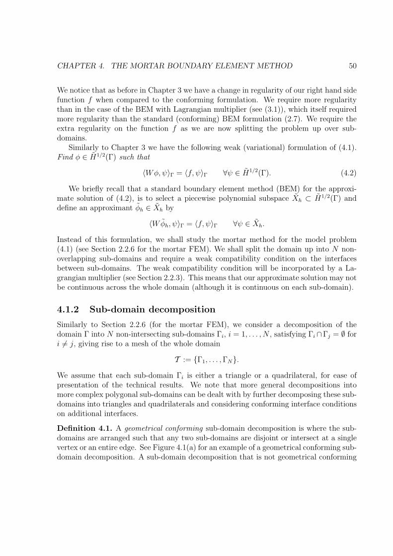
CHAPTER 4. THE MORTAR BOUNDARY ELEMENT METHOD 50
We notice that as before in Chapter 3 we have a change in regularity of our right hand sidefunction f when compared to the conforming formulation. We require more regularitythan in the case of the BEM with Lagrangian multiplier (see (3.1)), which itself requiredmore regularity than the standard (conforming) BEM formulation (2.7). We require theextra regularity on the function f as we are now splitting the problem up over sub-domains.
Similarly to Chapter 3 we have the following weak (variational) formulation of (4.1).Find φ ∈ H1/2(Γ) such that
〈Wφ,ψ〉Γ = 〈f, ψ〉Γ ∀ψ ∈ H1/2(Γ). (4.2)
We briefly recall that a standard boundary element method (BEM) for the approxi-mate solution of (4.2), is to select a piecewise polynomial subspace Xh ⊂ H1/2(Γ) anddefine an approximant φh ∈ Xh by
〈Wφh, ψ〉Γ = 〈f, ψ〉Γ ∀ψ ∈ Xh.
Instead of this formulation, we shall study the mortar method for the model problem(4.1) (see Section 2.2.6 for the mortar FEM). We shall split the domain up into N non-overlapping sub-domains and require a weak compatibility condition on the interfacesbetween sub-domains. The weak compatibility condition will be incorporated by a La-grangian multiplier (see Section 2.2.3). This means that our approximate solution may notbe continuous across the whole domain (although it is continuous on each sub-domain).
4.1.2 Sub-domain decomposition
Similarly to Section 2.2.6 (for the mortar FEM), we consider a decomposition of thedomain Γ into N non-intersecting sub-domains Γi, i = 1, . . . , N , satisfying Γi∩Γj = ∅ fori 6= j, giving rise to a mesh of the whole domain
T := Γ1, . . . ,ΓN.
We assume that each sub-domain Γi is either a triangle or a quadrilateral, for ease ofpresentation of the technical results. We note that more general decompositions intomore complex polygonal sub-domains can be dealt with by further decomposing these sub-domains into triangles and quadrilaterals and considering conforming interface conditionson additional interfaces.
Definition 4.1. A geometrical conforming sub-domain decomposition is where the sub-domains are arranged such that any two sub-domains are disjoint or intersect at a singlevertex or an entire edge. See Figure 4.1(a) for an example of a geometrical conforming sub-domain decomposition. A sub-domain decomposition that is not geometrical conforming
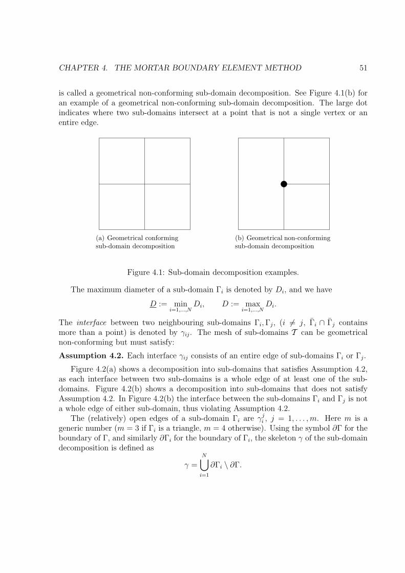
CHAPTER 4. THE MORTAR BOUNDARY ELEMENT METHOD 51
is called a geometrical non-conforming sub-domain decomposition. See Figure 4.1(b) foran example of a geometrical non-conforming sub-domain decomposition. The large dotindicates where two sub-domains intersect at a point that is not a single vertex or anentire edge.
(a) Geometrical conformingsub-domain decomposition
(b) Geometrical non-conformingsub-domain decomposition
Figure 4.1: Sub-domain decomposition examples.
The maximum diameter of a sub-domain Γi is denoted by Di, and we have
D := mini=1,...,N
Di, D := maxi=1,...,N
Di.
The interface between two neighbouring sub-domains Γi,Γj, (i 6= j, Γi ∩ Γj containsmore than a point) is denoted by γij. The mesh of sub-domains T can be geometricalnon-conforming but must satisfy:
Assumption 4.2. Each interface γij consists of an entire edge of sub-domains Γi or Γj.
Figure 4.2(a) shows a decomposition into sub-domains that satisfies Assumption 4.2,as each interface between two sub-domains is a whole edge of at least one of the sub-domains. Figure 4.2(b) shows a decomposition into sub-domains that does not satisfyAssumption 4.2. In Figure 4.2(b) the interface between the sub-domains Γi and Γj is nota whole edge of either sub-domain, thus violating Assumption 4.2.
The (relatively) open edges of a sub-domain Γi are γji , j = 1, . . . ,m. Here m is ageneric number (m = 3 if Γi is a triangle, m = 4 otherwise). Using the symbol ∂Γ for theboundary of Γ, and similarly ∂Γi for the boundary of Γi, the skeleton γ of the sub-domaindecomposition is defined as
γ =N⋃
i=1
∂Γi \ ∂Γ.
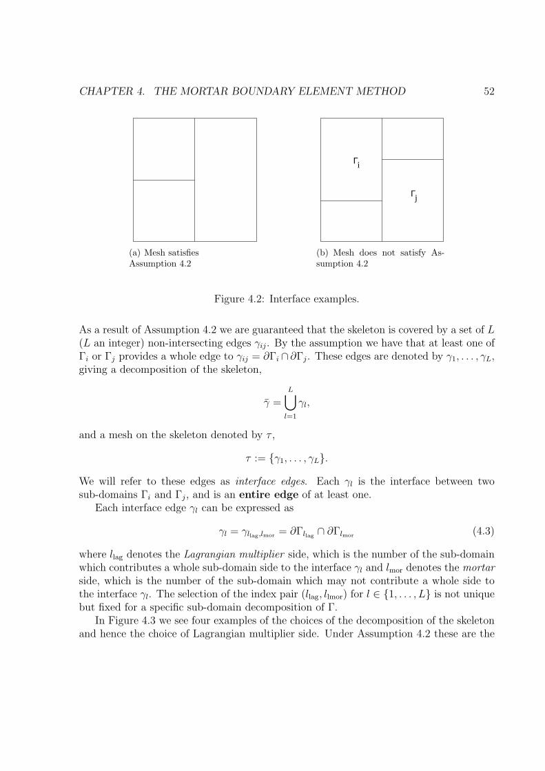
CHAPTER 4. THE MORTAR BOUNDARY ELEMENT METHOD 52
(a) Mesh satisfiesAssumption 4.2
Γ
Γj
i
(b) Mesh does not satisfy As-sumption 4.2
Figure 4.2: Interface examples.
As a result of Assumption 4.2 we are guaranteed that the skeleton is covered by a set of L(L an integer) non-intersecting edges γij. By the assumption we have that at least one ofΓi or Γj provides a whole edge to γij = ∂Γi ∩ ∂Γj. These edges are denoted by γ1, . . . , γL,giving a decomposition of the skeleton,
γ =L⋃
l=1
γl,
and a mesh on the skeleton denoted by τ ,
τ := γ1, . . . , γL.
We will refer to these edges as interface edges. Each γl is the interface between twosub-domains Γi and Γj, and is an entire edge of at least one.
Each interface edge γl can be expressed as
γl = γllag,lmor = ∂Γllag ∩ ∂Γlmor (4.3)
where llag denotes the Lagrangian multiplier side, which is the number of the sub-domainwhich contributes a whole sub-domain side to the interface γl and lmor denotes the mortarside, which is the number of the sub-domain which may not contribute a whole side tothe interface γl. The selection of the index pair (llag, llmor) for l ∈ 1, . . . , L is not uniquebut fixed for a specific sub-domain decomposition of Γ.
In Figure 4.3 we see four examples of the choices of the decomposition of the skeletonand hence the choice of Lagrangian multiplier side. Under Assumption 4.2 these are the
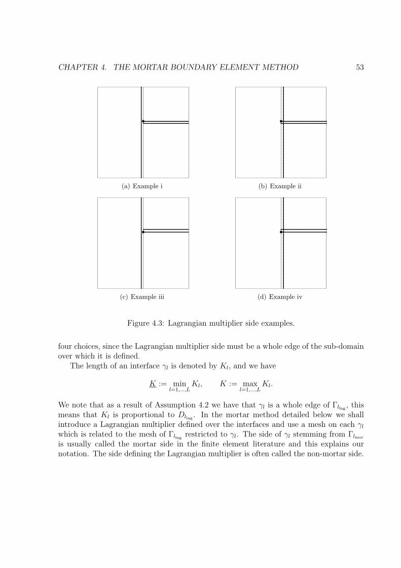
CHAPTER 4. THE MORTAR BOUNDARY ELEMENT METHOD 53
(a) Example i (b) Example ii
(c) Example iii (d) Example iv
Figure 4.3: Lagrangian multiplier side examples.
four choices, since the Lagrangian multiplier side must be a whole edge of the sub-domainover which it is defined.
The length of an interface γl is denoted by Kl, and we have
K := minl=1,...,L
Kl, K := maxl=1,...,L
Kl.
We note that as a result of Assumption 4.2 we have that γl is a whole edge of Γllag , thismeans that Kl is proportional to Dllag . In the mortar method detailed below we shallintroduce a Lagrangian multiplier defined over the interfaces and use a mesh on each γlwhich is related to the mesh of Γllag restricted to γl. The side of γl stemming from Γlmor
is usually called the mortar side in the finite element literature and this explains ournotation. The side defining the Lagrangian multiplier is often called the non-mortar side.
CHAPTER 4. THE MORTAR BOUNDARY ELEMENT METHOD 54
For the decomposition of Γ we need the product Sobolev space
Hs(T ) :=∏
K∈T
Hs(K) =N∏
i=1
Hs(Γi)
with usual product norm
‖ϕ‖2Hs(T ) =
N∑
i=1
‖ϕi‖2Hs(Γi)
.
We shall define curlH and curlH as follows for sufficiently smooth v and ϕ:
curlH ϕ =N∑
i=1
(curlΓiϕi)
0 , curlHϕ =N∑
i=1
(curlΓiϕi)
0 .
Where curlΓi, curlΓi
are defined as in Chapter 2 and the notation (·)0 indicates extensionby zero over the whole of Γ. We shall use the notation
〈·, ·〉T :=N∑
i=1
〈·, ·〉Γi
〈·, ·〉τ :=L∑
l=1
〈·, ·〉γl.
Here for a domain S ⊂ Γ or an arc S the notation 〈·, ·〉S denotes the L2(S)-inner productand its extension by duality. We also use the notations 〈·, ·〉T and 〈·, ·〉τ for duality pairingsof product space corresponding to the given decompositions T and τ . The notation [ϕ]denotes the jump of the function ϕ across γ, by this we mean
[ϕ]|γl= ϕllag |γl
− ϕlmor |γl, l = 1, . . . , L.
4.1.3 Integration by parts
Following Chapter 3 (and [25]) we now examine an integration-by-parts formula for thehypersingular operator. For a smooth scalar function ψ and a smooth tangential vectorfield ϕ, integration by parts applied on a sub-domain using (2.46) gives
〈curlΓiψ,ϕ〉Γi
= 〈ψ, curlΓiϕ〉Γi
− 〈ψ,ϕ · ti〉∂Γi, i = 1, . . . , N.
Here, ti is the unit tangential vector on ∂Γi (oriented mathematically positive whenidentifying Γi with a subset of IR2 which is compatible with the identification of Γ as a

CHAPTER 4. THE MORTAR BOUNDARY ELEMENT METHOD 55
subset of IR2). Applying this formula to ϕ = (V curlΓ φ)|Γi(restricted to Γi), we obtain
for smooth functions ψ and φ
〈ti · V curlΓ φ, ψi〉∂Γi= 〈curlΓi
V curlΓ φ, ψi〉Γi− 〈V curlΓ φ, curlΓi
ψi〉Γi.
Now we sum over i and take into account that ti = −tj on γij. Further we let γ0 := ∂Γ,the boundary of the whole domain , use the convention for the jump
[ψ]|γ0 = ψ|γ0 ,
denote by t0 the unit tangential vector along ∂Γ (again mathematically positive oriented)and let 0lag := 0 (remember the notation llag and lmor for the numbers of the Lagrangianmultiplier side and mortar side of γl, respectively). To put this another way for anysub-domain Γi such that ∂Γ ∩ ∂Γi 6= ∅ we define the jump over the interface γ0|∂Γi
as
[ψ]|γ0|∂Γi= ψ0lag
|γ0|∂Γi− ψ0mor |γ0|∂Γi
.
We then set ψ0lag|γ0|∂Γi
= ψi|γ0|∂Γiand ψ0mor|γ0|∂Γi
= 0. This gives us that
[ψ]|γ0|∂Γi= ψi|γ0|∂Γi
.
Now summing over all sub-domains Γi such that ∂Γ ∩ ∂Γi 6= ∅ we have that
[ψ]|γ0 = ψ|γ0 .
This yields
L∑
l=0
〈tllag · V curlΓ φ, [ψ]〉γl=
N∑
i=1
〈curlΓiV curlΓ φ, ψi〉Γi
−N∑
i=1
〈V curlΓ φ, curlΓiψi〉Γi
= 〈curlΓ V curlΓ φ, ψ〉T − 〈V curlΓ φ, curlH ψ〉T
for a piecewise (with respect to T ) smooth function ψ on Γ with ψi := ψ|Γi, as defined
before. Here, more precisely the notation curlΓiV curlΓ φ means curlΓi
(V curlΓ φ)|Γi.
Also, in the last step we used the fact that
curlH ϕ = curlΓ ϕ ∀ϕ ∈H1/2t (Γ),
which holds by a density argument and the continuity of curlΓ : H1/2t (Γ) → H−1/2(Γ) as
the adjoint operator of curlΓ : H1/2(Γ) → H−1/2
t (Γ), cf. Lemma 2.17.Now we use the relation
Wφ = curlΓ V curlΓ φ (φ ∈ H1/2(Γ)),
CHAPTER 4. THE MORTAR BOUNDARY ELEMENT METHOD 56
see [40, 43] and Lemma 2.20. Then choosing a piecewise smooth function ψ with ψ|∂Γ = 0we obtain
〈λ, [ψ]〉τ =L∑
l=1
〈λ, [ψ]〉γl= 〈Wφ,ψ〉T − 〈V curlΓ φ, curlH ψ〉T . (4.4)
Here, λ denotes our Lagrangian multiplier on the skeleton γ defined by
λ|γl:= tllag · (V curlΓ φ)|γl
, l = 1, . . . , L. (4.5)
Relation (4.4) does not extend to ψ ∈ H1/2(T ) since the trace of such a function v onto γis not well defined (see Lemma 2.22, Trace Theorem). However, there holds the followinglemma.
Lemma 4.3. For φ ∈ H1/2(Γ) with Wφ = f ∈ L2(Γ), (4.4) defines λ ∈∏L
l=1H−s(γl) for
any s ∈ (0, 1/2].
Remark 4.4. The above lemma can be extended to values of s larger than 1/2. Thoughsmall values of s represent the interesting cases, the limit s = 0 being excluded. Also, thecondition on f can be relaxed but excluding the case f ∈ H−1/2(Γ) which is the standardregularity using the mapping properties of the hypersingular operator.
Proof of Lemma 4.3. We must show that λ defined by (4.4) is a bounded linearfunctional on
∏Ll=1 H
s(γl), the dual space of∏L
l=1H−s(γl).
Let ψ ∈∏L
l=1 Hs(γl) be given. We continuously extend ψ to an element ψ ∈ Hs+1/2(T )
with ψ = 0 on ∂Γ such that [ψ]|γl= ψ|γl
. (Simply extend ψ on each interface edge γl to afunction in Hs+1/2(Γllag) vanishing on ∂Γllag \γl and extend by zero to the rest of Γ. Thensum up with respect to l.) The definition of λ is independent of the particular extensionψ, see Lemma 2.16 for details in the case of one sub-domain. Using a duality estimate weobtain from (4.4)
L∑
l=0
〈λ, [ψ]〉γl= 〈f, ψ〉T − 〈V curlΓ φ, curlH ψ〉T
≤ ‖f‖L2(Γ)‖ψ‖L2(Γ) +N∑
i=1
‖V curlΓ φ‖H1/2−st (Γi)
‖ curlΓiψi‖Hs−1/2
t (Γi).(4.6)
Now, for s ∈ (0, 1/2] the norms in H1/2−s
t (Γi) and H1/2−st (Γi) are equivalent (cf., e.g.,
[38]) so that together with the mapping property of V [19],
V : H−1/2−s
t (Γ) →H1/2−st (Γ),
CHAPTER 4. THE MORTAR BOUNDARY ELEMENT METHOD 57
and Lemma 2.17 we obtain
N∑
i=1
‖V curlΓ φ‖2
H1/2−st (Γi)
.
N∑
i=1
‖V curlΓ φ‖2
H1/2−st (Γi)
. ‖V curlΓ φ‖2
H1/2−st (Γ)
. ‖φ‖2H1/2(Γ)
.
Here, the appearing constants are independent of φ but may depend on s. Also, usingLemma 2.19 we are able to bound (with constant independent of ψ)
N∑
i=1
‖ curlΓiψi‖
2
Hs−1/2t (Γi)
.
N∑
i=1
‖ψi‖2Hs+1/2(Γi)
= ‖ψ‖2Hs+1/2(T ).
Taking the last two estimates into account, (4.6) proves that
L∑
l=1
〈λ, [ψ]〉γl.(‖f‖L2(Γ) + ‖φ‖H1/2(Γ)
)‖ψ‖Hs+1/2(T ).
Using the continuity of the extension (with constant independent of ψ)
‖ψ‖2Hs+1/2(T ) .
L∑
l=1
‖ψ‖2Hs(γl)
finishes the proof.
4.2 Discrete Variational Formulation of the Mortar
BEM
In this section we first present the meshes and discrete spaces that shall be used to definethe mortar BEM. We then present the discrete formulation of the mortar BEM.
4.2.1 Meshes and Discrete Spaces
On each Γi (i ∈ 1, . . . , N) we consider a sequence of regular, quasi-uniform meshes Ticonsisting of shape regular elements which are either triangles or quadrilaterals. Thisgives us that Γi = ∪T∈Ti
T , where T is an element of the mesh and T is the closure ofthe element, i.e. we include the boundary. The maximum diameter of elements of Ti isdenoted hi < 1 and we use
h := mini=1,...,N
hi, h := maxi=1,...,N
hi.
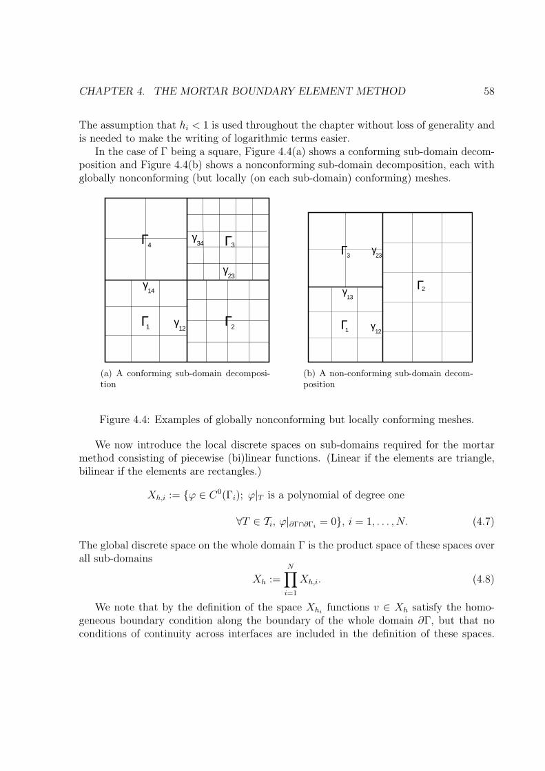
CHAPTER 4. THE MORTAR BOUNDARY ELEMENT METHOD 58
The assumption that hi < 1 is used throughout the chapter without loss of generality andis needed to make the writing of logarithmic terms easier.
In the case of Γ being a square, Figure 4.4(a) shows a conforming sub-domain decom-position and Figure 4.4(b) shows a nonconforming sub-domain decomposition, each withglobally nonconforming (but locally (on each sub-domain) conforming) meshes.
Γ Γ
Γ Γ
1 2
34
γ
γ
γ14
23
34
12γ
(a) A conforming sub-domain decomposi-tion
Γ
Γ
1
γ
12γ
Γ2
γ3
13
23
(b) A non-conforming sub-domain decom-position
Figure 4.4: Examples of globally nonconforming but locally conforming meshes.
We now introduce the local discrete spaces on sub-domains required for the mortarmethod consisting of piecewise (bi)linear functions. (Linear if the elements are triangle,bilinear if the elements are rectangles.)
Xh,i := ϕ ∈ C0(Γi); ϕ|T is a polynomial of degree one
∀T ∈ Ti, ϕ|∂Γ∩∂Γi= 0, i = 1, . . . , N. (4.7)
The global discrete space on the whole domain Γ is the product space of these spaces overall sub-domains
Xh :=N∏
i=1
Xh,i. (4.8)
We note that by the definition of the space Xhifunctions v ∈ Xh satisfy the homo-
geneous boundary condition along the boundary of the whole domain ∂Γ, but that noconditions of continuity across interfaces are included in the definition of these spaces.

CHAPTER 4. THE MORTAR BOUNDARY ELEMENT METHOD 59
As a result of this these functions are in general discontinuous across sub-domain inter-faces, and as such are in general not continuous functions on Γ. Therefore, Xh is not asubspace of the energy space H1/2(Γ) (functions in H1/2(Γ) are continuous across sub-domain interfaces). As noted before a standard BEM (2.8) chooses as a trial space asubspace of the energy space, which we are not doing here. Instead we shall incorporatethe continuity condition across sub-domain interfaces in a weak manner by the inclusionof a Lagrangian multiplier. Functions from different sub-domains will be coupled via adiscrete Lagrangian multiplier on the skeleton. This means that our functions will notin general be continuous across sub-domain interfaces but will have this discontinuityconstrained in some fashion. This shall cause us to have a non-standard method, andas shall be noted we have an error estimate with two parts (see Lemma 2.6). One partcomes from the conforming part of the method and the second part shows the effect ofthe discontinuities in the approximating function over interfaces on the error.
A mesh on the skeleton γ is needed to define the discrete Lagrangian multiplier space.On each interface edge γl we define a trace mesh Tllag |γl
being the restriction of the meshTllag from the sub-domain Γllag to the interface γl. We recall that by definition γl is awhole edge of Tllag . This inherited trace mesh is quasi-uniform with mesh width hllag . Themesh used to define the Lagrangian multiplier space Gl is a coarsening of the trace meshTllag |γl
, such that the following assumption is satisfied.
Assumption 4.5. For any l ∈ 1, . . . , L there holds: the mesh Gl is a strict coarseningof the trace mesh Tllag |γl
. The mesh Gl is made up of non-overlapping elements (straightline pieces) that satisfy:
• The elements extreme points are different nodes of Tllag |γl, and
• the interior of any element covers at least one interior node of Tllag |γl, which is a
different node to the extreme nodes of the element.
Figure 4.5 shows how we define our discrete Lagrangian multiplier space. The soliddots represent the restriction to the interface of the mesh of the sub-domain that has beenchosen as the Lagrangian multiplier side. The hollow circles represent the choice of nodesfor the Lagrangian multiplier space. The dashed lines then represent the Lagrangianmultipliers themselves. In Figure 4.5(a) we have an even number of nodes of the meshof the sub-domain restricted to the interface. We therefore define one of the intervals(the first) of our Lagrangian multiplier space as longer than the others in order to satisfyAssumption 4.5.
The mesh width (length of longest element) of Gl is denoted by kl, and
k := minl=1,...,L
kl, k := maxl=1,...,L
kl.
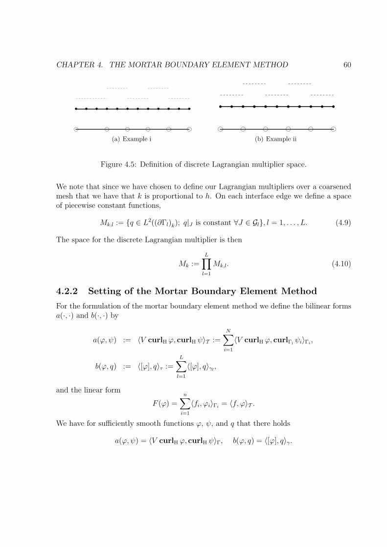
CHAPTER 4. THE MORTAR BOUNDARY ELEMENT METHOD 60
(a) Example i (b) Example ii
Figure 4.5: Definition of discrete Lagrangian multiplier space.
We note that since we have chosen to define our Lagrangian multipliers over a coarsenedmesh that we have that k is proportional to h. On each interface edge we define a spaceof piecewise constant functions,
Mk,l := q ∈ L2((∂Γl)k); q|J is constant ∀J ∈ Gl, l = 1, . . . , L. (4.9)
The space for the discrete Lagrangian multiplier is then
Mk :=L∏
l=1
Mk,l. (4.10)
4.2.2 Setting of the Mortar Boundary Element Method
For the formulation of the mortar boundary element method we define the bilinear formsa(·, ·) and b(·, ·) by
a(ϕ, ψ) := 〈V curlH ϕ, curlH ψ〉T :=N∑
i=1
〈V curlH ϕ, curlΓiψi〉Γi
,
b(ϕ, q) := 〈[ϕ], q〉τ :=L∑
l=1
〈[ϕ], q〉γl,
and the linear form
F (ϕ) =n∑
i=1
〈fi, ϕi〉Γi= 〈f, ϕ〉T .
We have for sufficiently smooth functions ϕ, ψ, and q that there holds
a(ϕ, ψ) = 〈V curlH ϕ, curlH ψ〉Γ, b(ϕ, q) = 〈[ϕ], q〉γ.
CHAPTER 4. THE MORTAR BOUNDARY ELEMENT METHOD 61
The mortar boundary element method for the approximate solution of (4.1) isthen: Find φh ∈ Xh and λk ∈Mk such that
a(φh, ψ) + b(ψ, λk) = F (ψ) ∀ψ ∈ Xh
b(φh, q) = 0 ∀q ∈Mk.(4.11)
This scheme is equivalent to:Find φh ∈ Vh such that
a(φh, ψ) = F (ψ) ∀ψ ∈ Vh, (4.12)
whereVh = ψ ∈ Xh : b(ψ, q) = 0 ∀q ∈Mk . (4.13)
We shall refer to Xh as an unconstrained space and Vh as a constrained space to indicatethe inclusion of the compatibility constraint in the definition of Vh.
4.3 Technical Details and Proof of the Main Result
In this section we present the analysis which leads to our main error result. Continuityand ellipticity of the bilinear form a(·, ·) are essential for the error analysis of the problemdescribed in equation (4.11), so we shall now examine these properties of the bilinear forma(·, ·). For completeness we show dependence of these results upon sub-domain size. Weshall first present the continuity and then the ellipticity.
Continuity of a(·, ·)
Lemma 4.6. The bilinear form a(·, ·) is almost uniformly continuous on Xh, there holds
|a(v, w)| . D−2| log(h/D)|2 ‖v‖H1/2(T ) ‖w‖H1/2(T ) ∀v, w ∈ Xh.
Proof. First we note that for v, w ∈ Xh ⊂ L2(Γ) there holds V curlH v ∈ L2t (Γ) so that
〈V curlH v, curlHw〉T = 〈V curlH v, curlHw〉Γ.
Now, using the continuity of V : H−1/2
t (Γ) → H1/2t (Γ) and the estimate for fractional
order Sobolev norms ‖ · ‖H
−1/2t (Γ)
. ‖ · ‖H
−1/2t (T )
, we obtain for v, w ∈ Xh
a(v, w) = 〈V curlH v, curlHw〉Γ . ‖ curlH v‖H−1/2t (Γ)
‖ curlHw‖H−1/2t (Γ)
. ‖ curlH v‖H−1/2t (T )
‖ curlHw‖H−1/2t (T )
. (4.14)
CHAPTER 4. THE MORTAR BOUNDARY ELEMENT METHOD 62
Now examining on each sub-domain and transforming to a reference sub-domain by (2.54),using Lemma 2.18 and Lemma 2.30, then transforming back by (2.48) we see that, forv ∈ Xh
‖ curlΓivi‖
2
H−1/2t (Γi)
. ‖ curlΓivi‖
2
H−1/2t (Γi)
. | log(hi/Di)|2‖ curlΓi
vi‖2
H−1/2t (Γi)
. | log(hi/Di)|2‖vi‖
2H1/2(Γi)
. D−2i | log(hi/Di)|
2‖vi‖2H1/2(Γi)
.
Giving us that
‖ curlH v‖H−1/2t (T )
. D−1| log(h/D)|‖v‖H1/2(T ) ∀v ∈ Xh.
Combination with (4.14) proves the statement.
Lemma 4.6 is not applicable to non-discrete functions. In particular this means wecannot use it when we consider the continuous function that is the solution of our modelproblem. For the error estimate of the mortar BEM we will require continuity for con-tinuous functions, we therefore need a different continuity estimate for our bilinear forma(·, ·), this is given in the following lemma.
Lemma 4.7. Assume that u ∈ H1/2+r(Γ) (r > 0). Then there holds
a(u− v, w) . D−1s−1‖u− v‖H1/2+s(T )‖ curlHw‖H−1/2t (T )
∀v, w ∈ Xh, ∀s ∈ (0,minr, 1/2].
In particular, the appearing constant is independent of s.
Proof. We note that (4.14) holds for continuous and discrete functions, so that for allv, w ∈ Xh and u ∈ H1/2+r(Γ) (r > 0) we have
a(u− v, w) . ‖curlH(u− v)‖H
−1/2t (T )
‖ curlHw‖H−1/2t (T )
. (4.15)
Now using (2.54), the continuous injection H−1/2+s
t (Γi) → H−1/2
t (Γi), Lemma 2.29, the
continuity of curlΓi: H1/2+s(Γi) →H
−1/2+st (Γi) by Lemma 2.18 and (2.48) we can bound
for i ∈ 1, . . . , N
‖ curlΓi(ui − vi)‖
2
H−1/2t (Γi)
. ‖ curlΓi(ui − vi)‖
2
H−1/2t (Γi)
. ‖ curlΓi(ui − vi)‖
2
H−1/2+st (Γi)
. s−2‖ curlΓi(ui − vi)‖
2
H−1/2+st (Γi)
. s−2‖ui − vi‖2H1/2+s(Γi)
. D−2i s−2‖ui − vi‖
2H1/2+s(Γi)
.

CHAPTER 4. THE MORTAR BOUNDARY ELEMENT METHOD 63
Summing over all sub-domains gives us that
‖curlH(u− v)‖H
−1/2t (T )
. D−1s−1‖u− v‖H1/2+s(T ).
Combination with (4.15) finishes the proof.
Before being able to prove Vh ellipticity we require an extension to the following result,which is a generalized version of a discrete Poincare-Friedrichs inequality in fractionalorder Sobolev spaces, Theorem 8 in [30].
Proposition 4.8. There exists a constant C > 0, independent of the decomposition Tas long as sub-domains are shape regular, such that for all ǫ ∈ (0, 1/2] there holds ∀v ∈H1/2+ǫ(T )
‖v‖2L2(Γ) ≤ C
(ǫ−1|v|2H1/2+ǫ(T ) +
L∑
l=1
K−1−2ǫl (
∫
γl
[v] ds)2
).
Where, Kl is the length of γl.
For a proof of Proposition 4.8 see Appendix A. In Lemma 4.9 we adapt the result ofProposition 4.8 to our mortar situation.
Lemma 4.9. For all v ∈ Vh
‖ curlH v‖2
H−1/2t (Γ)
& D| log(h/D)|−1‖v‖2H1/2(T ).
Proof. We first recall that for any v ∈ Vh we have, by definition (see (4.13)), the interfacematching condition
∫γl[v]µ ds = 0 for all µ ∈ Mk. We thus have that
∫γl[v] ds = 0 for
any interface edge γl since by construction Mk contains a constant function which hasthe value 1 on γl and vanishes on γ \ γl. Therefore Proposition 4.8 proves that (note theresult is independent of sub-domain size)
‖v‖2L2(Γ) . ǫ−1
n∑
i=1
|vi|2H1/2+ǫ(Γi)
∀v ∈ Vh. (4.16)
Here the appearing constant is independent of ǫ ∈ (0, 1/2]. Making use of (2.47), theinverse property and again (2.47) we bound
N∑
i=1
|v|2H1/2+ǫ(Γi).
N∑
i=1
D1−2ǫi |v|2
H1/2+ǫ(Γi).
N∑
i=1
D1−2ǫi (hi/Di)
−2ǫ|v|2H1/2(Γi)
.
N∑
i=1
D1−2ǫi D−1
i (hi/Di)−2ǫ|v|2H1/2(Γi)
∀v ∈ Vh. (4.17)
CHAPTER 4. THE MORTAR BOUNDARY ELEMENT METHOD 64
Combining (4.16) and (4.17) we have that (recalling ǫ ∈ (0, 1/2])
‖v‖2L2(Γ) . ǫ−1
n∑
i=1
D−2ǫi (hi/Di)
−2ǫ|vi|2H1/2(Γi)
. ǫ−1
n∑
i=1
D−1i (hi/Di)
−2ǫ|vi|2H1/2(Γi)
∀v ∈ Vh. (4.18)
Which holds since (assuming 0 < Di ≤ 1) D−2ǫi ≤ D−1
i . Now, for any v ∈ H1/2(T ) by(2.53), Lemma 2.19 and (2.47) there holds
‖ curlH v‖2
H−1/2t (Γ)
& ‖ curlH v‖2
H−1/2t (Γ)
&
N∑
i=1
‖ curlΓiv‖2
H−1/2t (Γi)
&
N∑
i=1
Di‖ curlΓivi‖
2
H−1/2t (Γi)
&
N∑
i=1
Di|vi|2H1/2(Γi)
&
N∑
i=1
DiD−1i |vi|
2H1/2(Γi)
&
N∑
i=1
|vi|2H1/2(Γi)
= |v|2H1/2(T ). (4.19)
We recall that‖v‖2
H1/2(T ) = ‖v‖2L2(T ) + |v|2H1/2(T ).
Combining (4.18) with (4.19) and selecting ǫ = | log(h/D)|−1 (for (h/D) being smallenough) proves the statement.
Ellipticity of a(·, ·)
We are now ready to prove the Vh-ellipticity of the bilinear form a(·, ·).
Lemma 4.10. The bilinear form a(·, ·) is almost uniformly Vh-elliptic, there holds:
a(v, v) & D| log(h/D)|−1 ‖v‖2H1/2(T ) ∀v ∈ Vh, (4.20)
and
a(v, v) & D1/2| log(h/D)|−1/2 ‖v‖H1/2(T ) ‖ curlH v‖H−1/2t (Γ)
∀v ∈ Vh. (4.21)
CHAPTER 4. THE MORTAR BOUNDARY ELEMENT METHOD 65
Proof. As in the proof of Lemma 4.6 we note that for v ∈ Vh ⊂ L2(Γ) there holds
〈V curlH v, curlH v〉T = 〈V curlH v, curlH v〉Γ.
Now for v ∈ Vh we have the following using the ellipticity of V : H− 1
2
t (Γ) → H12t (Γ) and
Lemma 4.9a(v, v) = 〈V curlH v, curlH v〉Γ
& ‖ curlH v‖2
H−1/2t (Γ)
& D| log(h/D)|−1‖v‖2H1/2(T )
.
Which gives (4.20). The estimate (4.21) is obtained by bounding ‖ curlH v‖H−1/2t (Γ)
only
once with Lemma 4.9.
In order to achieve a Strang-type error estimate (see Lemma 2.6) we shall need to ex-tend functions from interfaces onto sub-domains (see Lemma 2.14 for the mortar FEM).This shall also be required in the proof of the inf-sup condition. We now define exten-sion operators that extend piecewise linear functions from interface edges to piecewise(bi)linear functions on the corresponding Lagrangian sub-domain.
El : Xh,llag |γl→ Xh,llag , l = 1, . . . , L. (4.22)
Here for v ∈ Xh,llag |γl, the extension Elv is the function of Xh,llag that coincides with v in
the nodes on γl from the mesh Tllag and is zero in the remaining nodes of Tllag .
Lemma 4.11. For all v ∈ Xh,llag |γl, and for all s ∈ [0, 1], l = 1, . . . , L
‖Elv‖Hs(Γllag) . D
1/2llag
(hllag/Dllag)1/2−s‖v‖L2(γl).
In particular the appearing constant is independent of s.
Proof. Using the equivalence of norms in finite dimensional spaces and scaling propertiesof the L2-norm one obtains, by taking into account the construction of El and using (2.47),
‖Elv‖2L2(Γllag
) . D2llag
‖Elv‖2L2(Γllag
)
. D2llag
(hllag/Dllag)‖v‖2L2(γl)
. D2llag
(hllag/Dllag)K−1l ‖v‖2
L2(γl)
. Dllag(hllag/Dllag)‖v‖2L2(γl)
∀v ∈ Xh,llag |γl. (4.23)
In the above we have used that the interface γl (of length Kl) is a whole edge of thesub-domain Γllag and thus has length proportional to Dllag . Analogously we find using(2.47)
|Elv|2H1(Γllag
) . |Elv|2H1(Γllag
)
CHAPTER 4. THE MORTAR BOUNDARY ELEMENT METHOD 66
. (hllag/Dllag)−1|v|2H1(γl)
. (hllag/Dllag)−1Kl|v|
2H1(γl)
. Dllag(hllag/Dllag)−1|v|2H1(γl)
∀v ∈ Xh,llag |γl. (4.24)
We can now show by combining (4.23) and (4.24) that
‖Elv‖2H1(Γllag
) = ‖Elv‖2L2(Γllag
) + |Elv|2H1(Γllag
)
. Dllag
((hllag/Dllag)‖v‖
2L2(γl)
+ (hllag/Dllag)−1|v|2H1(γl)
)
. Dllag(hllag/Dllag)−1‖v‖2
H1(γl)∀v ∈ Xh,llag |γl
. (4.25)
The result then follows by interpolation between (4.23) and (4.25).
Inf-sup condition
Lemma 4.12. The bilinear form b(·, ·) satisfies the discrete inf-sup condition:
∃β > 0 : supv∈Xh
b(v, µ)
‖v‖H1/2(T )
≥ β‖µ‖L2(γ) ∀µ ∈Mk.
Proof. Let µ ∈Mk be given. On each interface edge γl, µ is a piecewise constant functionon Gl, a mesh that is coarser than the trace mesh Tllag |γl
stemming from the Lagrangianmultiplier side Γllag , cf. Assumption 4.5. On γl we construct a piecewise linear functionwl ∈ Xh,llag |γl
in the following way. For each element J ∈ Gl, wl vanishes at the endpointsof J , coincides with µ at one interior node of J and is linearly interpolated elsewhere onγl. See Figure 4.6 for an example where µ is represented by the dashed line and wl by thesolid line. The bullets indicate the nodes of the mesh for the Lagrangian multiplier andthe dashes indicate additional nodes of the trace mesh (from the Lagrangian multiplierside).
We then extend wl to wl in Xh by first extending to Elwl ∈ Xh,llag (cf. (4.22)) and
then further by zero onto Γ. Eventually we define v :=∑L
l=1 wl.Note that wl vanishes on all interface edges except γl. The trace of wl onto γl from
Γllag equals wl whereas the trace coming from the other side Γlmor vanishes. This yields
[v] = [wl] = wl on γl, l = 1, . . . , L. (4.26)
By the construction of wl there holds, uniformly for µ ∈Mk,
‖µ‖2L2(γl)
≃ 〈wl, µ〉γl≃ ‖wl‖
2L2(γl)
, l = 1, . . . , L. (4.27)

CHAPTER 4. THE MORTAR BOUNDARY ELEMENT METHOD 67
Also, taking into account that each sub-domain Γi has a limited number of (interface)edges, determined by the relation l ∈ 1, . . . , L : llag = i, Lemma 4.11 yields
‖v‖2H1/2(T ) =
N∑
i=1
∥∥∥∑
l∈1,...,L: llag=i
Elwl
∥∥∥2
H1/2(Γi)
.
N∑
i=1
∑
l∈1,...,L: llag=i
‖Elwl‖2H1/2(Γi)
=L∑
l=1
‖Elwl‖2H1/2(Γllag)
.
L∑
l=1
‖wl‖2L2(γl)
. (4.28)
Now, using (4.26), (4.27) and (4.28), we finish the proof by bounding
b(v, µ) =L∑
l=1
〈[v], µ〉γl=
L∑
l=1
〈wl, µ〉γl≃ ‖µ‖L2(γ)
( L∑
l=1
‖wl‖2L2(γl)
)1/2
& ‖µ‖L2(γ)‖v‖H1/2(T ).
(a) (b)
Figure 4.6: Construction of wl in the proof of Lemma 4.12.
Lemma 4.13. For all v ∈ Xh there holds
‖[v]‖2L2(γ) . D−1| log(h/D)|‖v‖2
H1/2(T ).
Proof. By the triangle inequality and Lemma 2.22 there holds uniformly for ǫ ∈ (0, 1/2)

CHAPTER 4. THE MORTAR BOUNDARY ELEMENT METHOD 68
and for any v ∈ Xh, using (2.52) and noting that Kl is proportional to Dllag
‖[v]‖2L2(γ) .
L∑
l=1
Kl
(‖vllag‖
2L2(γl)
+ ‖vlmor‖2L2(γl)
)
. ǫ−1
L∑
l=1
Kl
(‖vllag‖
2H1/2+ǫ(Γllag
)+ ‖vlmor‖
2H1/2+ǫ(Γlmor )
)
. ǫ−1
n∑
i=1
Di‖vi‖2H1/2+ǫ(Γi)
∀v ∈ Xh.
The inverse property, applied separately to vi = v|Γi, yields
n∑
i=1
‖vi‖2H1/2+ǫ(Γi)
.
n∑
i=1
(hi/Di)−2ǫ‖vi‖
2H1/2(Γi)
. D−2(h/D)−2ǫ‖v‖2H1/2(T ) ∀v ∈ Xh,
by an application of (2.48). Selecting ǫ = | log(h/D)|−1 (for (h/D) being small enough)finishes the proof.
Continuity of b(·, ·)
Lemma 4.14. The bilinear form b(·, ·) is almost uniformly discretely continuous, in thesense that
b(v, µ) . D−1/2| log(h/D)|1/2‖v‖H1/2(T )‖µ‖L2(γ) ∀v ∈ Xh,∀µ ∈Mk. (4.29)
Let ψ ∈ L2(γ) be given. Then there holds
b(v, ψ) . D−1| log(h/D)| infµ∈Mk
‖ψ − µ‖L2(γ)‖ curlH v‖H−1/2t (Γ)
∀v ∈ Vh. (4.30)
Proof. There holds
b(v, µ) =L∑
l=1
〈[v], µ〉γl≤ ‖[v]‖L2(γ)‖µ‖L2(γ) ∀v ∈ Xh,∀µ ∈Mk.
Estimate (4.29) follows with the help of Lemma 4.13. To prove (4.30) we start as beforeand note that by definition of Vh there holds b(v, µ) = 0 ∀µ ∈ Mk, ∀v ∈ Vh. Therefore,for any µ ∈Mk and v ∈ Vh, we find that for ψ ∈ L2(γ)
b(v, ψ) ≤ ‖[v]‖L2(γ)‖ψ − µ‖L2(γ). (4.31)
The proof of (4.30) is finished by noting that combination of Lemmas 4.13 and 4.9 yields
‖[v]‖L2(γ) . D−1/2| log(h/D)|1/2‖v‖H1/2(T ) . D−1| log(h/D)| ‖ curlH v‖H−1/2t (Γ)
∀v ∈ Vh.
CHAPTER 4. THE MORTAR BOUNDARY ELEMENT METHOD 69
Existence and uniqueness
We are now ready to prove the following Strang-type error estimate.
Theorem 4.15. The system (4.11) is uniquely solvable. For φ ∈ H1/2+r(Γ), r ∈ (0, 1/2],being the solution of (4.2), and φh ∈ Xh being the solution of (4.11) there holds
‖φ− φh‖H1/2(T ) . D−2| log(h/D)|1/2(s−1 inf
v∈Vh
‖φ− v‖H1/2+s(T )
+ supw∈Vh\0
|a(φ− φh, w)|
‖ curlHw‖H−1/2t (Γ)
)
uniformly for s ∈ (0, r].
Proof. The existence and uniqueness of (φh, λk) ∈ Xh ×Mk follows from the Babuska-Brezzi theory (see Section 2.2.4). Indeed, the bilinear form a(·, ·) is continuous on Xh
by Lemma 4.6 and Vh-elliptic by Lemma 4.10, and the bilinear form b(·, ·) is continuouson Xh × Mk by (4.29) and satisfies a discrete inf-sup condition by Lemma 4.12. Thecontinuity and ellipticity bounds depend on h and D but that does not influence theunique solvability of the discrete scheme.
The error estimate (c.f., Lemma 2.6) is obtained by the usual steps. Combining (2.49),the triangle inequality, (2.48), the non-standard ellipticity and continuity properties ofa(·, ·) (cf. (4.21) and Lemma 4.7) we obtain for any v ∈ Vh
‖φ− φh‖H1/2(T ) ≤ D−1/2‖φ− v‖H1/2(T ) + ‖v − φh‖H1/2(T )
. D−1/2
‖φ− v‖H1/2(T ) +D−1/2| log(h/D)|1/2 sup
w∈Vh\0
a(v − φh, w)
‖ curlHw‖H−1/2t (Γ)
≤ D−1/2
‖φ− v‖H1/2(T ) +D−1/2| log(h/D)|1/2
(sup
w∈Vh\0
a(v − φ,w)
‖ curlHw‖H−1/2t (Γ)
+ supw∈Vh\0
a(φ− φh, w)
‖ curlHw‖H−1/2t (Γ)
)
. D−1/2
D−1/2‖φ− v‖H1/2(T ) + s−1D−3/2| log(h/D)|1/2‖φ− v‖H1/2+s(T )
+D−1/2| log(h/D)|1/2 supw∈Vh\0
a(φ− φh, w)
‖ curlHw‖H−1/2t (Γ)
.
This proves the stated error bound.
CHAPTER 4. THE MORTAR BOUNDARY ELEMENT METHOD 70
In order to analyse the upper bound provided by Theorem 4.15 we need, in additionto the extension operators El defined before (in (4.22)), projection operators which haveparticular properties (see Lemma 2.13 for the mortar FEM situation). Let us defineprojection operators πl acting on L2(γl) and mapping onto special continuous, piecewiselinear functions on γl, l = 1, . . . , L. We recall that on each γl we have two meshes: thetrace mesh Tllag |γl
stemming from the mesh on the sub-domain Γllag of the Lagrangianside, and the mesh Gl for the Lagrangian multiplier. For each element J ∈ Gl we considera hat function φl,J that vanishes at the endpoints of J and has the tip at a node of Tllag |γl
that is interior to J . This choice is not unique if J contains more than two elements ofthe trace mesh. In that case we select an arbitrary but fixed node for the definition ofφl,J . Using this notation we define
πl : L2(γl) → spanφl,J ; J ∈ Gl ⊂ Xh,llag , l = 1, . . . , L, (4.32)
such that the integral mean zero conditions
〈v − πlv, 1〉J = 0 ∀J ∈ Gl, l = 1, . . . , L
hold. This operator satisfies the following properties:
Lemma 4.16. For any v ∈ L2(γl), πlv vanishes at the endpoints of γl, l = 1, . . . , L, andthere holds
〈v − πlv, µ〉γl= 0 ∀v ∈ L2(γl), ∀µ ∈Mk,l, l = 1, . . . , L, (4.33)
‖πlv‖L2(γl) . ‖v‖L2(γl) ∀v ∈ L2(γl), l = 1, . . . , L. (4.34)
Proof. For l ∈ 1, . . . , L let v ∈ L2(γl) be given. By definition of πl, πlv vanishes atthe endpoints of γl, and the orthogonality (4.33) follows by noting that any µ ∈ Mk,l isconstant on any J ∈ Gl.
To show (4.34) let J ∈ Gl be given. With φl,J being the hat function defined previously(with height 1) there holds
πlv =2
|J |(
∫
J
v ds) φl,J on J
so that
‖πlv‖2L2(J) =
4
3|J |(
∫
J
v ds)2 ≤4
3‖v‖2
L2(J).
Summing over J ∈ Gl finishes the proof.
We are now ready to analyse the first term of the upper bounds provided by Theo-rem 4.15.
CHAPTER 4. THE MORTAR BOUNDARY ELEMENT METHOD 71
Lemma 4.17. For r ∈ (0, 1/2] let φ ∈ H1/2+r(Γ). There holds
infv∈Vh
‖φ− v‖2H1/2+s(T ) . D−1−2s
‖φ− w‖2
H1/2+s(T )
+L∑
l=1
Dllag(hllag/Dllag)−2s(‖φ− wllag‖
2L2(γl)
+‖φ− wlmor‖2L2(γl)
)∀w ∈ Xh
uniformly for s ∈ (0, r].
Proof. Let w ∈ Xh be given. We adapt w such that the new function satisfies the jumpconditions defining Vh, cf. (4.13). We set
v := w +L∑
l=1
rl ∈ Xh
with
rl :=
Elπl(wllag |γl
− wlmor|γl) on Γllag ,
0 elsewhere.
Here, El and πl are the extension and projection operators specified in (4.22) and (4.32),respectively. Note that, since πl(wllag |γl
− wlmor|γl) vanishes at the endpoints of γl, the
extension Elπl(wllag |γl− wlmor |γl
) vanishes on ∂Γllag \ γl. Therefore, using (4.33) one im-mediately obtains
〈[v], µ〉γl= 〈vllag − vlmor , µ〉γl
= 〈wllag + rl − wlmor , µ〉γl
= 〈wllag − wlmor + πl(wllag |γl− wlmor|γl
), µ〉γl= 0 ∀µ ∈Mk,l, l = 1, . . . , L.
That is, v ∈ Vh. We start bounding the error by using (2.49), the triangle inequality and(2.48)
‖φ− v‖2H1/2+s(T ) =
N∑
i=1
∥∥∥φi − wi −∑
l∈1,...,L: llag=i
rl∥∥∥
2
H1/2+s(Γi)
. D−1−2s
N∑
i=1
‖φi − wi‖2H1/2+s(Γi)
+L∑
l=1
‖rl‖2H1/2+s(Γllag
)
.(4.35)
Applying Lemma 4.11, (4.34) and the triangle inequality we find that there holds
‖rl‖H1/2+s(Γllag) . D
1/2llag
(hllag/Dllag)−s‖πl(wllag |γl
− wlmor|γl)‖L2(γl)
CHAPTER 4. THE MORTAR BOUNDARY ELEMENT METHOD 72
. D1/2llag
(hllag/Dllag)−s‖wllag − wlmor‖L2(γl)
. D1/2llag
(hllag/Dllag)−s(‖φ− wllag‖L2(γl) + ‖φ− wlmor‖L2(γl)
). (4.36)
Combining (4.35) and (4.36) one obtains the assertion.
Error estimate
The next result proves an a-priori error estimate for the mortar BEM.
Theorem 4.18. Let φ and φh be the solutions of (4.2) and (4.11), respectively. Assumingthat φ ∈ H1/2+r(Γ) (r ∈ (0, 1/2]) there holds λ ∈
∏Ll=1H
r(γl) and we have the a priorierror estimate
‖φ− φh‖2H1/2(T ) . s−2D−5−2s| log(h/D)|
(‖φ− v‖2
H1/2+s(T )
+D(h/D)−2s
L∑
l=1
(‖φ− vllag‖
2L2(γl)
+ ‖φ− vlmor‖2L2(γl)
))
+ D−6| log(h/D)|3 ‖λ− µ‖2L2(γ) ∀v ∈ Xh, ∀µ ∈Mk
uniformly for s ∈ (0, r]. Here, λ is the Lagrangian multiplier defined by (4.4) and (4.5).
Proof. Since φ ∈ H1/2+r(Γ) there holds
λ|γl= tllag · (V curlΓ φ)|γl
∈ Hr(γl), l = 1, . . . , L.
To this end note that curlΓ : H1/2+r(Γ) → Hr−1/2
t (Γ) (combine Lemma 2.17 with the
continuity curlΓ : H10 (Γ) → L2
t (Γ)) and V : Hr−1/2
t (Γ) →H1/2+rt (Γ). The trace theorem
(Lemma 2.22) concludes the claimed regularity of λ. In particular there holds λ ∈ L2(γ).By definition of Vh, and making use of Lemma 4.3, we find
a(φ− φh, w) = a(φ,w) − F (w) = b(w, λ) ∀w ∈ Vh.
Application of (4.30) yields
a(φ− φh, w) . D−1| log(h/D)| infµ∈Mk
‖λ− µ‖L2(γ)‖ curlHw‖H−1/2t (Γ)
∀w ∈ Vh.
CHAPTER 4. THE MORTAR BOUNDARY ELEMENT METHOD 73
Therefore, combining Theorem 4.15 with Lemma 4.17 we obtain
‖φ− φh‖2H1/2(T ) . D−4| log(h/D)|
s−2D−1−2s
(‖φ− v‖2
H1/2+s(T )
+L∑
l=1
Dllag(hllag/Dllag)−2s(‖φ− vllag‖
2L2(γl)
+ ‖φ− vlmor‖2L2(γl)
))
+ D−2| log(h/D)|2 ‖λ− µ‖2L2(γ)
∀v ∈ Xh, ∀µ ∈Mk.
This proves the statement.
Main result
The following theorem is the main result concerning the mortar BEM.
Theorem 4.19. There exists a unique solution (φh, λk) of (4.11). Assume that the solu-tion φ of (4.2) satisfies φ ∈ H1/2+r(Γ) (r ∈ (0, 1/2]). Then there holds
‖φ− φh‖H1/2(T ) . D−4(| log(h/D)|2(h/D)r +D−3| log(h/D)|3/2(k/K)r)‖φ‖H1/2+r(Γ).
For proportional mesh sizes h and k this means that
‖φ− φh‖H1/2(T ) . D−4| log(h/D)|2(h/D)r‖φ‖H1/2+r(Γ).
Proof. By Theorem 4.15 the system (4.11) is uniquely solvable. We employ the generala priori estimate by Theorem 4.18 to show the given error bound. By standard approxi-mation theory there exist v ∈ Xh and µ ∈Mk such that (using (2.49) and (2.48))
n∑
i=1
‖φi − vi‖2H1/2+s(Γi)
.
n∑
i=1
D1−2si ‖φi − vi‖
2H1/2+s(Γi)
.
n∑
i=1
D1−2si (hi/Di)
2(r−s)‖φi‖2H1/2+r(Γi)
.
n∑
i=1
D1−2si (hi/Di)
2(r−s)D−2i ‖φi‖
2H1/2+r(Γi)
. D−1−2s(h/D)2(r−s)‖φ‖2H1/2+r(Γ)
. D−2(h/D)2(r−s)‖φ‖2H1/2+r(Γ)
, (4.37)
CHAPTER 4. THE MORTAR BOUNDARY ELEMENT METHOD 74
and (using (2.52) and (2.51))
‖λ− µ‖2L2(γ) .
L∑
l=1
Kl‖λ− µ‖2L2(γl)
.
L∑
l=1
Kl(kl/Kl)2r‖λ‖2
Hr(γl)
.
L∑
l=1
Kl(kl/Kl)2rK−1
l ‖λ‖2Hr(γl)
.
L∑
l=1
(kl/Kl)2r‖λ‖2
Hr(γl), (4.38)
and as in the proof of Theorem 4.18 we conclude that∑L
l=1 ‖λ‖2Hr(γl)
. ‖φ‖2H1/2+r(Γ)
. By
Lemma 2.22 we bound (recalling that Kl is proportional to Dllag)
‖φ− vllag‖L2(γl) . K1/2l ‖φ− vllag‖L2(γl)
. K1/2l s−1/2‖φ− v‖H1/2+s(Γllag
)
. K1/2l s−1/2(hllag/Dllag)
r−s‖φ‖H1/2+r(Γllag)
. K1/2l s−1/2(hllag/Dllag)
r−sD−1llag
‖φ‖H1/2+r(Γllag)
. D−1/2llag
s−1/2(hllag/Dllag)r−s‖φ‖H1/2+r(Γllag
), (4.39)
and accordingly the mortar part ‖φ − vlmor‖L2(γl). Since H1/2+r(Γ) ⊂ H1/2+r(Γ) we havethat
L∑
l=1
‖φ‖2H1/2+r(Γllag
) . ‖φ‖2H1/2+r(T ) . ‖φ‖2
H1/2+r(Γ).
Using these bounds in Theorem 4.18 and selecting s = | log(h/D)|−1 we obtain the asser-tion.
Remark 4.20. As in Remark 3.8 we note that, in our case of an open surface Γ, thesolution φ of (4.1) has strong corner and corner-edge singularities which cannot be exactlydescribed by standard Sobolev regularity. It is well-known that φ ∈ Hr(Γ) for any r < 1(see, e.g., [55]) so that the error estimate by Theorem 4.19 holds for any r < 1/2. Ingeneral φ 6∈ H1
0 (Γ) but a more specific error analysis for the conforming BEM yields forquasi-uniform meshes the optimal error estimate
‖φ− φh‖H1/2(Γ) . h1/2,
CHAPTER 4. THE MORTAR BOUNDARY ELEMENT METHOD 75
see [8]. The logarithmical perturbations in h and D of our error estimate are due tothe non-conformity of the mortar method. They stem from the non-existence of a traceoperator within H1/2(Γ) and from non-local properties of the fractional order Sobolevnorms (the difference between H1/2 and H1/2-spaces).
Remark 4.21. The mortar method may be able to be applied to other BEM boundaryconditions provided that certain necessary conditions are met. Firstly an appropriateintegration by parts formula involving surface differential operators is required to calcu-late the necessary interface matching conditions. Next the system would have to satisfyappropriate ellipticity and continuity conditions, including the Babuska-Brezzi condition.Finally suitable projection and extension operators acting on appropriate spaces wouldhave to exist.
Chapter 5
Numerical Results
In this chapter we present numerical results for the BEM with Lagrangian multiplier andthe mortar BEM. These results agree with the theory and give the expected rates ofconvergence. In the mortar BEM situation we consider sequences of meshes which arerefined on each individual sub-domain. This means that on each sub-domain the meshsize becomes smaller and smaller, however the decomposition of the whole domain intosub-domains remains fixed. Thus the sub-domain size remains the same throughout eachexperiment and we are only interested in the effect of the mesh size (on the sub-domains)on the convergence rate of the scheme.
5.1 An Error Estimate
We consider the model problems (3.1) and (4.20) (for the BEM with Lagrangian multiplierand the Mortar BEM respectively) with Γ = (0, 1)× (0, 1) and f = 1. The discretisationsfor the methods shall be discussed later in the relevant sections. Before proceeding to thiswe must first discuss the error estimate that is to be presented.
Implementing the scheme (3.5) in the Lagrangian multiplier situation (or (4.2) in themortar BEM situation) we calculate the approximation φh ∈ Vh ⊂ Xh to the exact solutionφ of (3.1) in the Lagrangian multiplier situation (or (4.1) in the mortar BEM situation).Since φ is unknown there is no direct way to calculate the error ‖φ − φh‖H1/2(Γ) in theLagrangian multiplier situation (or ‖φ−φh‖H1/2(T ) in the mortar BEM situation). Instead,we approximate an upper bound to the semi-norm |φ − φh|H1/2(Γ) in the Lagrangianmultiplier situation (or |φ− φh|H1/2(T )in the mortar BEM situation).
In the following we present the results for T where T = Γ in the situation of the BEMwith Lagrangian multiplier and T = T in the Mortar BEM situation. By Lemma 3.5(i)for the BEM with Lagrangian multiplier (or the proof of Lemma 4.9 for the mortar BEM)
76
CHAPTER 5. NUMERICAL RESULTS 77
there holdsa(φ− φh, φ− φh) & |φ− φh|
2H1/2(T ). (5.1)
Moreover, since φ solves (3.1) and φh solves (3.5) for the BEM with Lagrangian multiplier(or (4.1) and (4.2) for the mortar BEM respectively), we find that there holds
a(φ− φh, φ− φh) = a(φ, φ) − 2a(φ, φh) + a(φh, φh)
= 〈Wφ, φ〉Γ − 2a(φ, φh) + F (φh) − b(φh, λk)
= 〈Wφ, φ〉Γ + F (φh) − 2a(φ, φh).
Now for the BEM with Lagrangian multiplier situation we set
[φh] = φh|γ,
and use the standard jump notation for the mortar BEM (see (4.3)). For the BEM withLagrangian multiplier, as in (3.11) we can apply (3.4) (or by (4.4) for the mortar BEM)and we obtain
a(φ, φh) = F (φh) − 〈[φh], λ〉γ .
Such that, with the previous relation,
a(φ−φh, φ−φh) = 〈Wφ, φ〉Γ−F (φh)+2 〈[φh], λ〉γ ≤ 〈Wφ, φ〉Γ−F (φh)+2 ‖[φh]‖L2(γ)‖λ‖L2(γ).(5.2)
As in the proof of Theorem 3.7 for the BEM with Lagrangian multiplier (or Theorem 4.18for the mortar BEM) we establish that ‖λ‖L2(γ) is bounded by a constant depending onφ. Therefore, by (5.1) we find that
|φ− φh|2H1/2(T ) . |〈Wφ, φ〉Γ − F (φh)| + ‖[φh]‖L2(γ).
The terms F (φh) and ‖[φh]‖L2(γ) can be easily calculated and 〈Wφ, φ〉Γ can be approx-imated by an extrapolated value that we denote by ‖φ‖2
ex (cf. [23]). Therefore, instead ofthe relative error ‖φ− φh‖H1/2(T )/‖φ‖H1/2(Γ), we present results for the expression
(| ‖φ‖2
ex − F (φh)| + ‖[φh]‖L2(γ)
)1/2
/‖φ‖ex, (5.3)
which is, up to a constant factor, an upper bound for |φ−φh|H1/2(T )/‖φ‖ex. In the figuresbelow we show different error curves, indicated by numbers (n) (n = 1, . . . , 4) as follows.
(1)(| ‖φ‖2
ex − F (φh)| + ‖[φh]‖L2(γ)
)1/2
“Total approximation error”
(2)(| ‖φ‖2
ex − F (φh)|)1/2
“Part 1 of the error”
(3) ‖[φh]‖1/2
L2(γ) “Part 2 of the error”
(4) a(φ− φh, φ− φh)1/2 “Conforming BEM”.
CHAPTER 5. NUMERICAL RESULTS 78
Here, φh denotes a conforming boundary element solution. Additionally, all curvesare normalized by ‖φ‖ex. Therefore, to resume, an error curve (1) represents the upperbound (5.3) for the (normalized) error |φ − φh|H1/2(T ) of our approximation (BEM withLagrangian multiplier or mortar BEM). Curves (2) and (3) are the two components of(1). Here, (3) controls the non-conformity of the approximant φh. Curve (4) representsthe error of the conforming BEM. In this case it is equivalent to the error in energy norm‖φ− φh‖H1/2(Γ).
All results are plotted on double logarithmic scales versus 1/h. For our numericalexperiments we always use rectangular meshes for the mortar BEM, hi refers to thediameter of the longest element on Γi, and h := maxi hi as before. For the BEM withLagrangian multiplier we set Γi = Γ and so h refers to the diameter of the longest elementon Γ.
General remarks
Let us note that the part ‖[φh]‖1/2γ of the error expression (5.3) is an overestimation.
Indeed, our substitution (5.3) for |φ − φh|H1/2(T )/‖φ‖ex is not precise. On the one handwe replaced the term 2 ‖λ‖L2(γ) in (5.2) by 1 (and the generic constant in (5.1) by 1).
On the other hand in the BEM with Lagrangian multiplier situation the term 〈t ·V curlΓ φ, φh〉γ is of higher order than ‖φh‖L2(γ). According to the proof of Theorem 3.7(see (3.11) and (3.13)) there holds
|〈t · V curlΓ φ, φh〉γ| ≤ C k1/2−ǫ‖φ‖H1−ǫ(Γ)‖φh‖L2(γ)
= C (2h)1/2−ǫ‖φ‖H1−ǫ(Γ)‖φh‖L2(γ) (ǫ > 0).
Equivalently in the Mortar BEM situation we have that 〈[φh], λ〉γ is of higher order than‖[φh]‖L2(γ). According to (4.31) and by standard approximation theory there holds forany r < 1/2
|〈[φh], λ〉γ| . ‖[φh]‖L2(γ) infψ∈Mk
‖λ− ψ‖L2(γ) . kr(L∑
l=1
|λ|2Hr(γl))1/2‖[φh]‖L2(γ).
This shows that 〈[φh], λ〉γ is of higher order than ‖[φh]‖L2(γ). Note that, by the proof of
Theorem 4.18 and since φ ∈ H1/2+r(Γ), we have the regularity λ ∈∏L
l=1Hr(γl) ∀r <
1/2. Therefore, by the above and (5.2) the term
(| ‖φ‖ex − F (φh)|
)1/2
/‖φ‖ex (curve (2), “Part 1 of error”)
is asymptotically equal toa(φ− φh, φ− φh)
1/2/‖φ‖ex.

CHAPTER 5. NUMERICAL RESULTS 79
5.2 BEM With Lagrangian Multiplier
In the case of the BEM with Lagrangian multiplier the meshes Th are uniform consistingof squares of side-length h and for each Th we select the mesh Gk which is compatible withTh|γ (as required by Theorem 3.7) with k = 2h (see Figure 5.1 where the bullets indicatethe nodes of Gk).These meshes define the boundary element space Xh and the space Mk
for the Lagrangian multiplier.
k
h
Figure 5.1: Uniform meshes Th and Gk.
As can be seen, the curve (1) in Figure 5.2 is parallel to the curve indicated by (4) whichgives the errors in H1/2(Γ) of the corresponding conforming method (i.e. Vh ⊂ H1/2(Γ)using the same meshes). Actually, for φ ∈ H1/2(Γ), ‖φ‖2
H1/2(Γ)and a(φ, φ) are equivalent
and the latter expression is used. Both errors, (1) and (4), behave like O(h1/2) whosecurve is also given. In this way the result of Theorem 3.7 is underlined.
Note, however, that we do not observe an ǫ-perturbation (reduced convergenceO(h1/2−ǫ)) nor a poly-logarithmic perturbation in 1/h. The absence of an ǫ-perturbationis expected, cf. Remark 3.8. The absence of a poly-logarithmic perturbation in h in thisrange of unknowns can be caused by the fact that we did not take the L2(Γ) part of theerror in H1/2(Γ) into account since our results are, up to constant factors, upper boundsonly for the semi-norm |u− uh|H1/2(Γ) (see Lemma 3.5(i)). Also, we do not know whetherour bounds including the logarithmic terms are sharp.
Considering the results in Figure 5.2 it appears that the errors of the BEM withLagrangian multiplier are much larger than those of the conforming method. This is nottrue for our model problem. This is since, as discussed previously, that the part ‖φh‖
1/2
L2(γ)
of the error expression (5.3) is an overestimation. We recall that we have that(|〈Wφ, φ〉Γ − 〈f, φh〉Γ|
)1/2
/‖φ‖ex “Part 1 of error”,
is asymptotically equal toa(φ− φh, φ− φh)
1/2/‖φ‖ex,
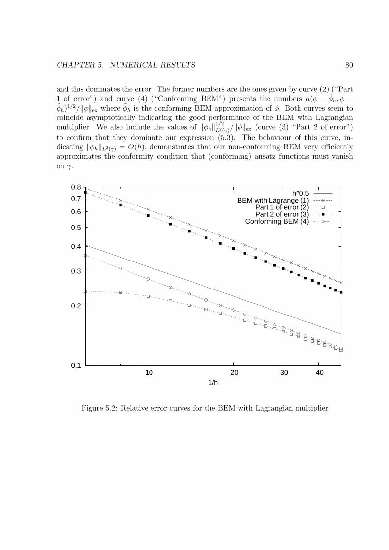
CHAPTER 5. NUMERICAL RESULTS 80
and this dominates the error. The former numbers are the ones given by curve (2) (“Part1 of error”) and curve (4) (“Conforming BEM”) presents the numbers a(φ − φh, φ −φh)
1/2/‖φ‖ex where φh is the conforming BEM-approximation of φ. Both curves seem tocoincide asymptotically indicating the good performance of the BEM with Lagrangianmultiplier. We also include the values of ‖φh‖
1/2
L2(γ)/‖φ‖ex (curve (3) “Part 2 of error”)
to confirm that they dominate our expression (5.3). The behaviour of this curve, in-dicating ‖φh‖L2(γ) = O(h), demonstrates that our non-conforming BEM very efficientlyapproximates the conformity condition that (conforming) ansatz functions must vanishon γ.
0.1
0.2
0.3
0.4
0.5
0.6
0.7
0.8
0.1 10 20 30 40 10
1/h
h^0.5BEM with Lagrange (1)
Part 1 of error (2)Part 2 of error (3)
Conforming BEM (4)
Figure 5.2: Relative error curves for the BEM with Lagrangian multiplier
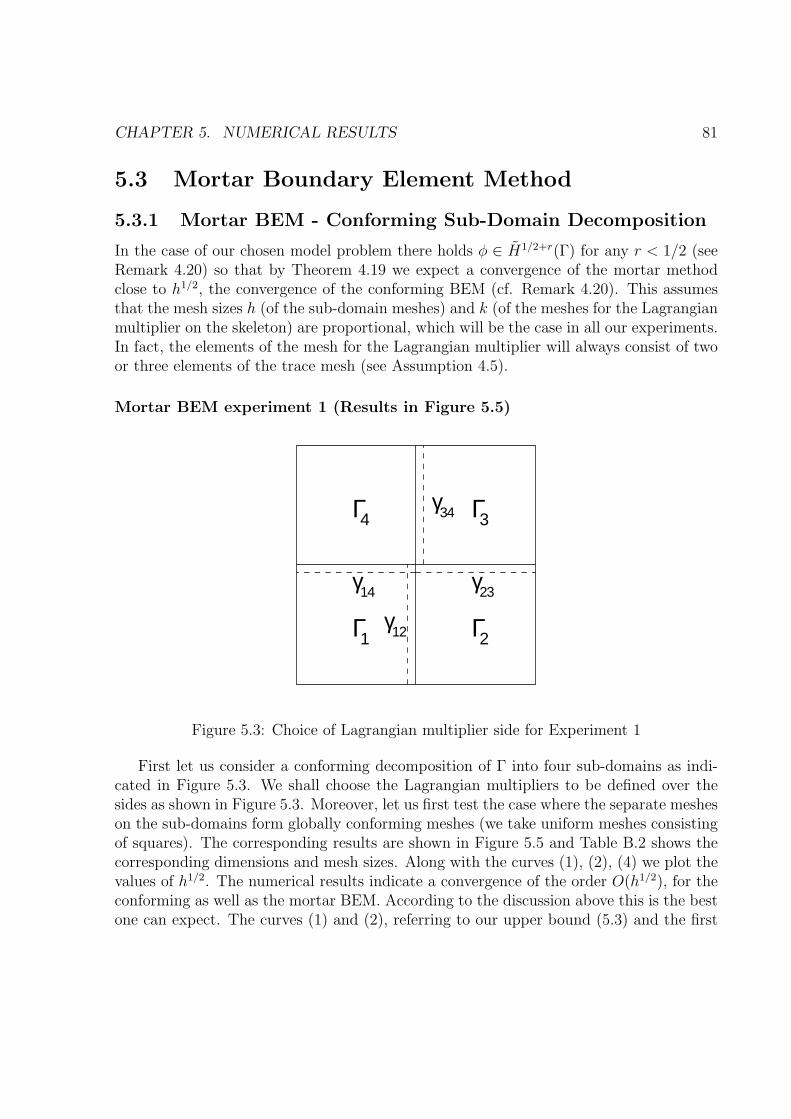
CHAPTER 5. NUMERICAL RESULTS 81
5.3 Mortar Boundary Element Method
5.3.1 Mortar BEM - Conforming Sub-Domain Decomposition
In the case of our chosen model problem there holds φ ∈ H1/2+r(Γ) for any r < 1/2 (seeRemark 4.20) so that by Theorem 4.19 we expect a convergence of the mortar methodclose to h1/2, the convergence of the conforming BEM (cf. Remark 4.20). This assumesthat the mesh sizes h (of the sub-domain meshes) and k (of the meshes for the Lagrangianmultiplier on the skeleton) are proportional, which will be the case in all our experiments.In fact, the elements of the mesh for the Lagrangian multiplier will always consist of twoor three elements of the trace mesh (see Assumption 4.5).
Mortar BEM experiment 1 (Results in Figure 5.5)
ΓΓ
Γ Γ1 2
34
γ
γ
γ
γ14
12
23
34
Figure 5.3: Choice of Lagrangian multiplier side for Experiment 1
First let us consider a conforming decomposition of Γ into four sub-domains as indi-cated in Figure 5.3. We shall choose the Lagrangian multipliers to be defined over thesides as shown in Figure 5.3. Moreover, let us first test the case where the separate mesheson the sub-domains form globally conforming meshes (we take uniform meshes consistingof squares). The corresponding results are shown in Figure 5.5 and Table B.2 shows thecorresponding dimensions and mesh sizes. Along with the curves (1), (2), (4) we plot thevalues of h1/2. The numerical results indicate a convergence of the order O(h1/2), for theconforming as well as the mortar BEM. According to the discussion above this is the bestone can expect. The curves (1) and (2), referring to our upper bound (5.3) and the first
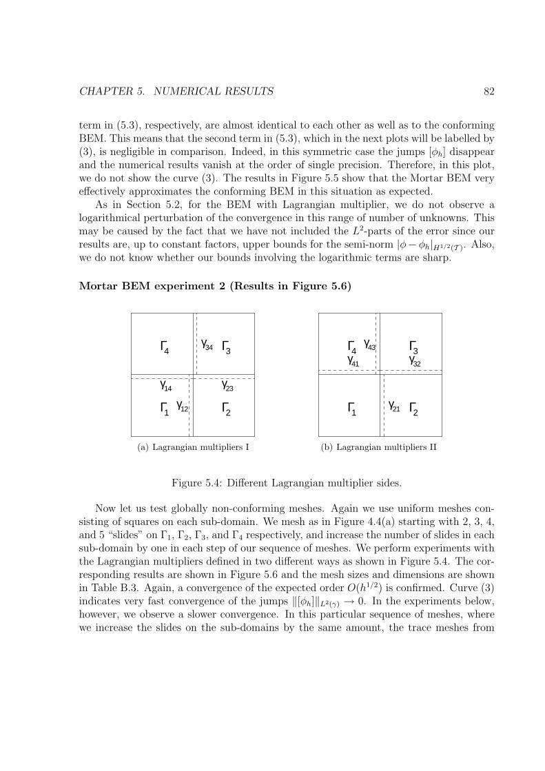
CHAPTER 5. NUMERICAL RESULTS 82
term in (5.3), respectively, are almost identical to each other as well as to the conformingBEM. This means that the second term in (5.3), which in the next plots will be labelled by(3), is negligible in comparison. Indeed, in this symmetric case the jumps [φh] disappearand the numerical results vanish at the order of single precision. Therefore, in this plot,we do not show the curve (3). The results in Figure 5.5 show that the Mortar BEM veryeffectively approximates the conforming BEM in this situation as expected.
As in Section 5.2, for the BEM with Lagrangian multiplier, we do not observe alogarithmical perturbation of the convergence in this range of number of unknowns. Thismay be caused by the fact that we have not included the L2-parts of the error since ourresults are, up to constant factors, upper bounds for the semi-norm |φ− φh|H1/2(T ). Also,we do not know whether our bounds involving the logarithmic terms are sharp.
Mortar BEM experiment 2 (Results in Figure 5.6)
ΓΓ
Γ Γ1 2
34
γ
γ
γ
γ14
12
23
34
(a) Lagrangian multipliers I
ΓΓ
Γ Γ1 2
34
γ
γγ43
γ41 32
21
(b) Lagrangian multipliers II
Figure 5.4: Different Lagrangian multiplier sides.
Now let us test globally non-conforming meshes. Again we use uniform meshes con-sisting of squares on each sub-domain. We mesh as in Figure 4.4(a) starting with 2, 3, 4,and 5 “slides” on Γ1, Γ2, Γ3, and Γ4 respectively, and increase the number of slides in eachsub-domain by one in each step of our sequence of meshes. We perform experiments withthe Lagrangian multipliers defined in two different ways as shown in Figure 5.4. The cor-responding results are shown in Figure 5.6 and the mesh sizes and dimensions are shownin Table B.3. Again, a convergence of the expected order O(h1/2) is confirmed. Curve (3)indicates very fast convergence of the jumps ‖[φh]‖L2(γ) → 0. In the experiments below,however, we observe a slower convergence. In this particular sequence of meshes, wherewe increase the slides on the sub-domains by the same amount, the trace meshes from
CHAPTER 5. NUMERICAL RESULTS 83
different sides on a particular interface edge approach each other in a certain sense. Weconjecture that this specific situation (“approaching” conforming meshes) causes the fastconvergence of the jumps.
Mortar BEM experiment 3 (Results in Figure 5.7)
For the next experiment we start with a mesh of four squares on each sub-domain (the sub-domains are again as in Figure 4.4(a)), and increase the numbers of slides on different sub-domains by different steps (increase by 2, 3, 4, 5 slides on Γ1, Γ2, Γ3, and Γ4 respectively).The results are shown in Figure 5.7 and the corresponding mesh sizes and dimensions areshown in Table B.4. In this case both error parts, curves (2) and (3), behave like O(h1/2),thus confirming the good performance of the mortar BEM.
In Figure 5.7 we clearly see the effect that defining the Lagrangian multiplier in adifferent way has on the performance of the method. We see that in particular situationsthis can actually be quite a dramatic change. While, as expected, the choice of Lagrangianmultipliers has little effect on ”Part 1 of the error” it has a large effect on ”Part 2 of theerror”. This is expected since it is the second part of the error which measures the errorcontributed by the jumps of the functions over the interfaces. The large differences in thetwo curves (3) are likely caused by the different choices of Lagrangian multiplier sides. Inexperiment II we choose the Lagrangian multiplier sides as shown in Figure 5.4(b). Ofparticular note we choose the Lagrangian multipliers to be defined over the restrictionsof Γ4 to the bounding interfaces. This means that we are choosing the sub-domain withthe finest mesh thus making the Lagrangian multipliers as numerous as possible. Thedifferences in the curves (3) appear to be particularly large when we have an even numberof slides on all sub-domains. This could be because we are close to a conforming situation.
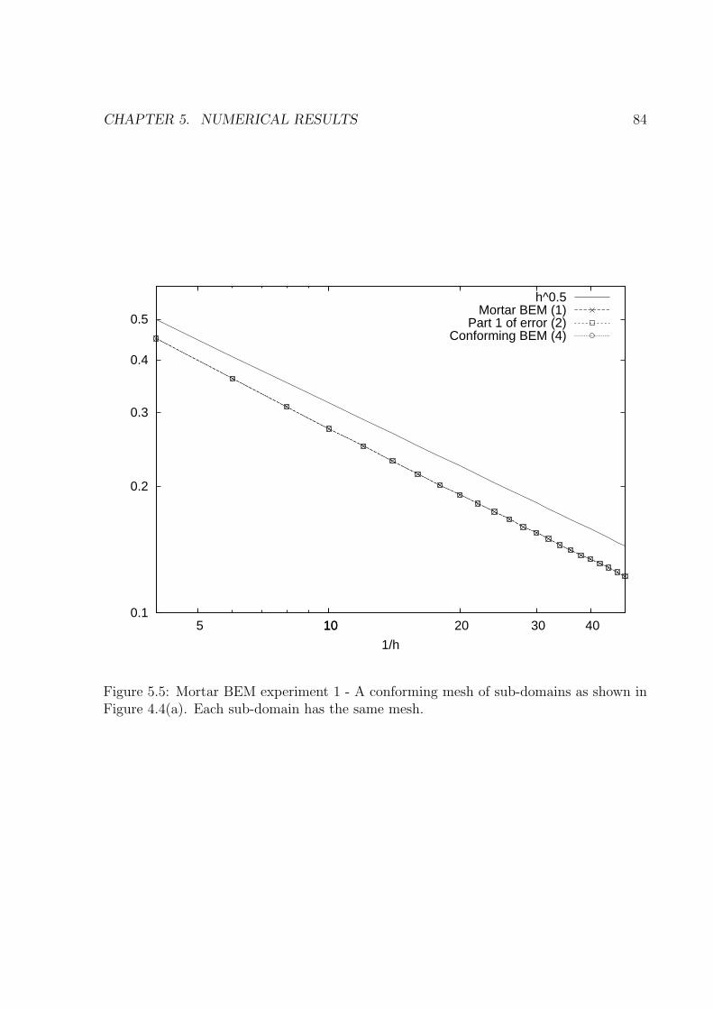
CHAPTER 5. NUMERICAL RESULTS 84
0.1
0.2
0.3
0.4
0.5
5 10 20 30 40 10
1/h
h^0.5Mortar BEM (1)
Part 1 of error (2)Conforming BEM (4)
Figure 5.5: Mortar BEM experiment 1 - A conforming mesh of sub-domains as shown inFigure 4.4(a). Each sub-domain has the same mesh.
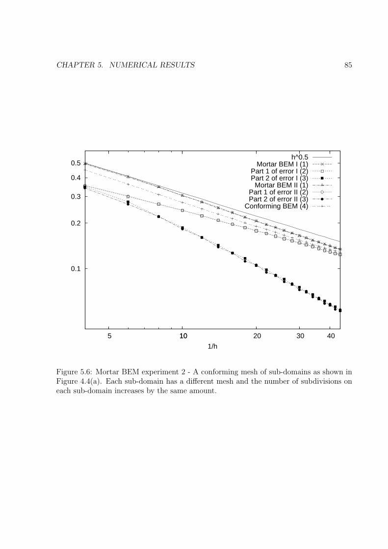
CHAPTER 5. NUMERICAL RESULTS 85
0.1
0.2
0.3
0.4
0.5
5 10 20 30 40 10
1/h
h^0.5Mortar BEM I (1)
Part 1 of error I (2)Part 2 of error I (3)
Mortar BEM II (1)Part 1 of error II (2)Part 2 of error II (3)
Conforming BEM (4)
Figure 5.6: Mortar BEM experiment 2 - A conforming mesh of sub-domains as shown inFigure 4.4(a). Each sub-domain has a different mesh and the number of subdivisions oneach sub-domain increases by the same amount.
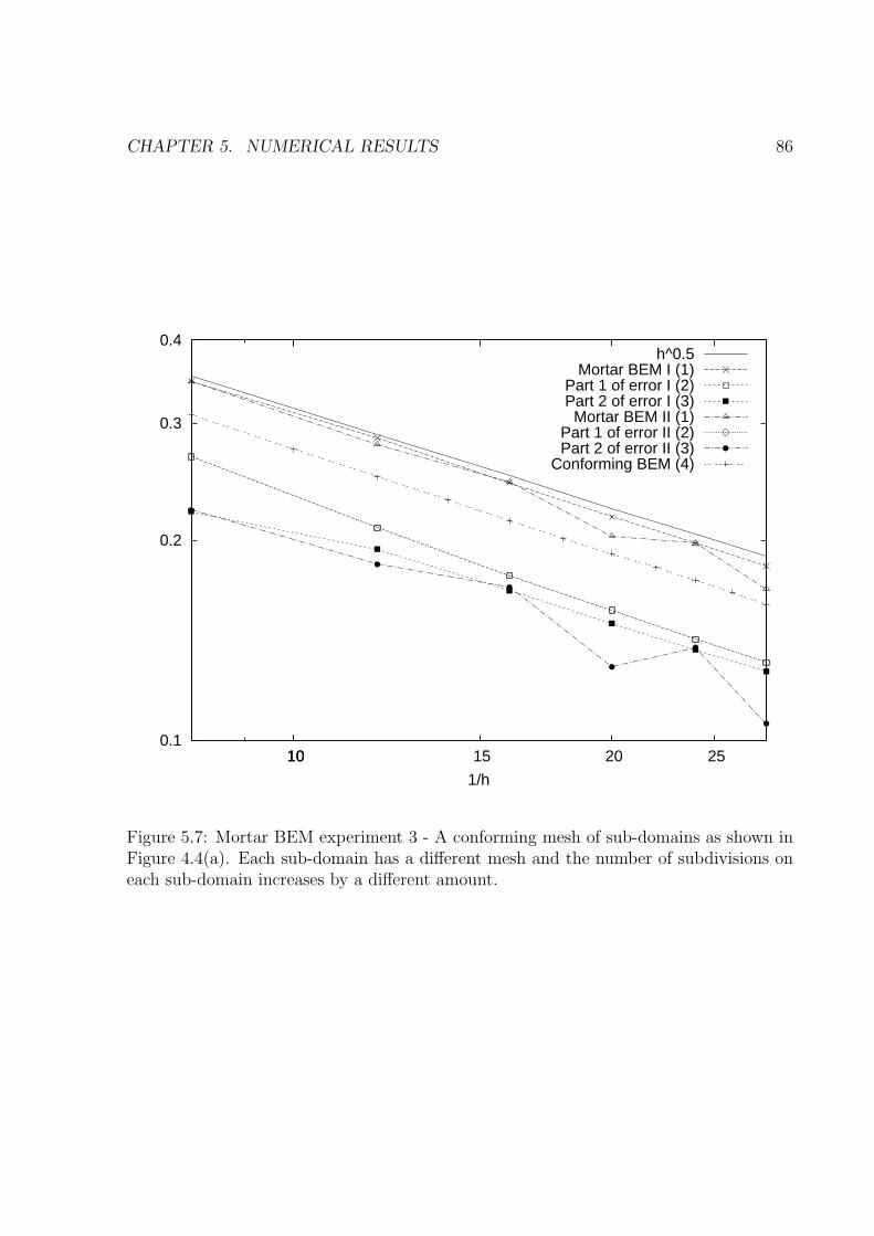
CHAPTER 5. NUMERICAL RESULTS 86
0.1
0.2
0.3
0.4
10 15 20 25 10
1/h
h^0.5Mortar BEM I (1)
Part 1 of error I (2)Part 2 of error I (3)
Mortar BEM II (1)Part 1 of error II (2)Part 2 of error II (3)
Conforming BEM (4)
Figure 5.7: Mortar BEM experiment 3 - A conforming mesh of sub-domains as shown inFigure 4.4(a). Each sub-domain has a different mesh and the number of subdivisions oneach sub-domain increases by a different amount.
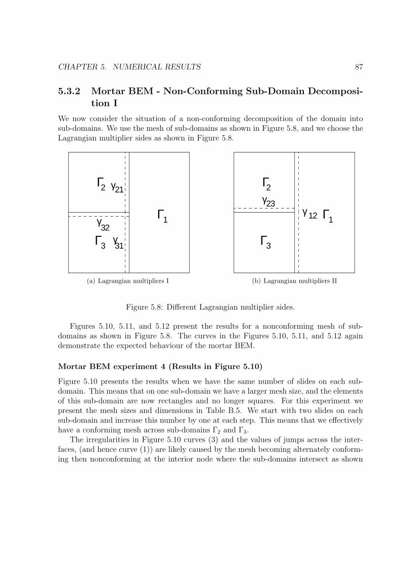
CHAPTER 5. NUMERICAL RESULTS 87
5.3.2 Mortar BEM - Non-Conforming Sub-Domain Decomposi-tion I
We now consider the situation of a non-conforming decomposition of the domain intosub-domains. We use the mesh of sub-domains as shown in Figure 5.8, and we choose theLagrangian multiplier sides as shown in Figure 5.8.
Γ
Γ
Γγ 1
2
3
21γ
32γ31
(a) Lagrangian multipliers I
Γ
Γ
Γ1
2
3
γγ
1223
(b) Lagrangian multipliers II
Figure 5.8: Different Lagrangian multiplier sides.
Figures 5.10, 5.11, and 5.12 present the results for a nonconforming mesh of sub-domains as shown in Figure 5.8. The curves in the Figures 5.10, 5.11, and 5.12 againdemonstrate the expected behaviour of the mortar BEM.
Mortar BEM experiment 4 (Results in Figure 5.10)
Figure 5.10 presents the results when we have the same number of slides on each sub-domain. This means that on one sub-domain we have a larger mesh size, and the elementsof this sub-domain are now rectangles and no longer squares. For this experiment wepresent the mesh sizes and dimensions in Table B.5. We start with two slides on eachsub-domain and increase this number by one at each step. This means that we effectivelyhave a conforming mesh across sub-domains Γ2 and Γ3.
The irregularities in Figure 5.10 curves (3) and the values of jumps across the inter-faces, (and hence curve (1)) are likely caused by the mesh becoming alternately conform-ing then nonconforming at the interior node where the sub-domains intersect as shown
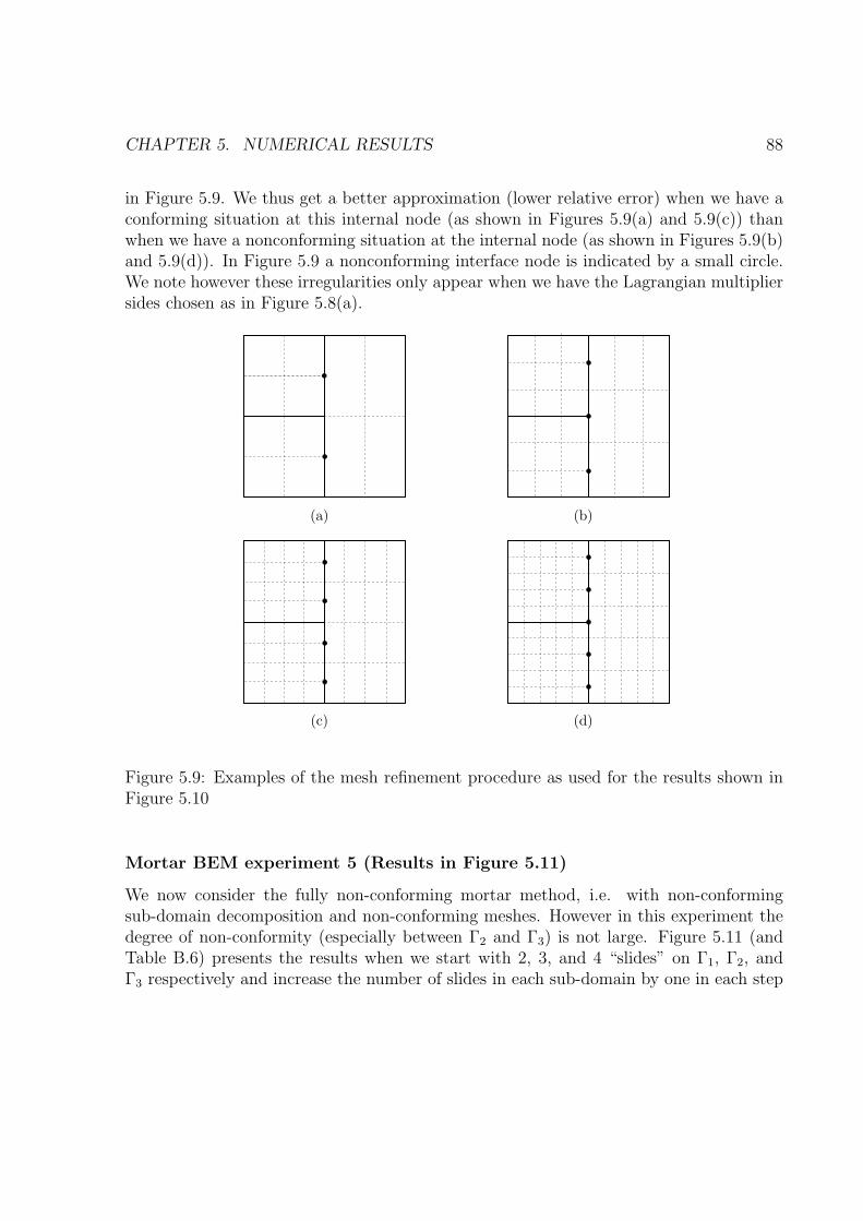
CHAPTER 5. NUMERICAL RESULTS 88
in Figure 5.9. We thus get a better approximation (lower relative error) when we have aconforming situation at this internal node (as shown in Figures 5.9(a) and 5.9(c)) thanwhen we have a nonconforming situation at the internal node (as shown in Figures 5.9(b)and 5.9(d)). In Figure 5.9 a nonconforming interface node is indicated by a small circle.We note however these irregularities only appear when we have the Lagrangian multipliersides chosen as in Figure 5.8(a).
(a) (b)
(c) (d)
Figure 5.9: Examples of the mesh refinement procedure as used for the results shown inFigure 5.10
Mortar BEM experiment 5 (Results in Figure 5.11)
We now consider the fully non-conforming mortar method, i.e. with non-conformingsub-domain decomposition and non-conforming meshes. However in this experiment thedegree of non-conformity (especially between Γ2 and Γ3) is not large. Figure 5.11 (andTable B.6) presents the results when we start with 2, 3, and 4 “slides” on Γ1, Γ2, andΓ3 respectively and increase the number of slides in each sub-domain by one in each step
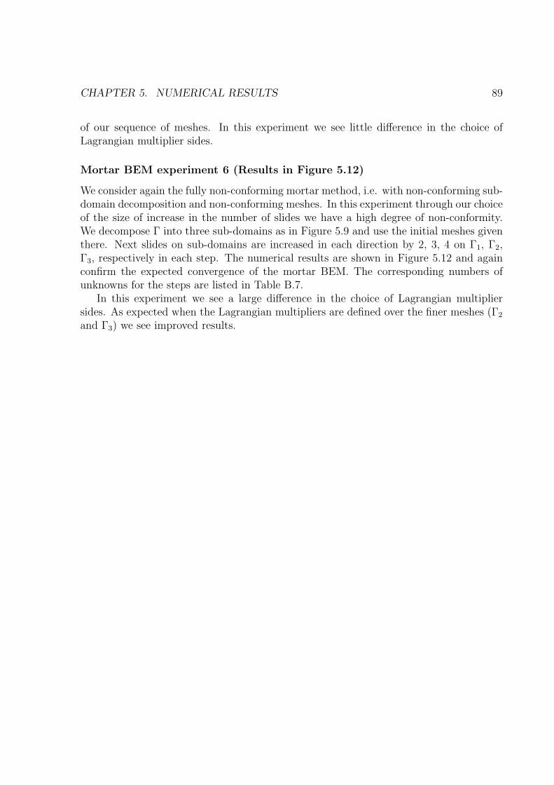
CHAPTER 5. NUMERICAL RESULTS 89
of our sequence of meshes. In this experiment we see little difference in the choice ofLagrangian multiplier sides.
Mortar BEM experiment 6 (Results in Figure 5.12)
We consider again the fully non-conforming mortar method, i.e. with non-conforming sub-domain decomposition and non-conforming meshes. In this experiment through our choiceof the size of increase in the number of slides we have a high degree of non-conformity.We decompose Γ into three sub-domains as in Figure 5.9 and use the initial meshes giventhere. Next slides on sub-domains are increased in each direction by 2, 3, 4 on Γ1, Γ2,Γ3, respectively in each step. The numerical results are shown in Figure 5.12 and againconfirm the expected convergence of the mortar BEM. The corresponding numbers ofunknowns for the steps are listed in Table B.7.
In this experiment we see a large difference in the choice of Lagrangian multipliersides. As expected when the Lagrangian multipliers are defined over the finer meshes (Γ2
and Γ3) we see improved results.

CHAPTER 5. NUMERICAL RESULTS 90
0.1
0.2
0.3
0.4
0.5
0.6
0.7
0.8 0.9
1
2 5 10 15 20 27 10
1/h
h^0.5Mortar BEM I (1)
Part 1 of error I (2)Part 2 of error I (3)
Mortar BEM II (1)Part 1 of error II (2)Part 2 of error II (3)
Figure 5.10: Mortar BEM experiment 4 - A nonconforming mesh of sub-domains as shownin Figure 4.4(b). Each sub-domain has the same number of subdivisions.
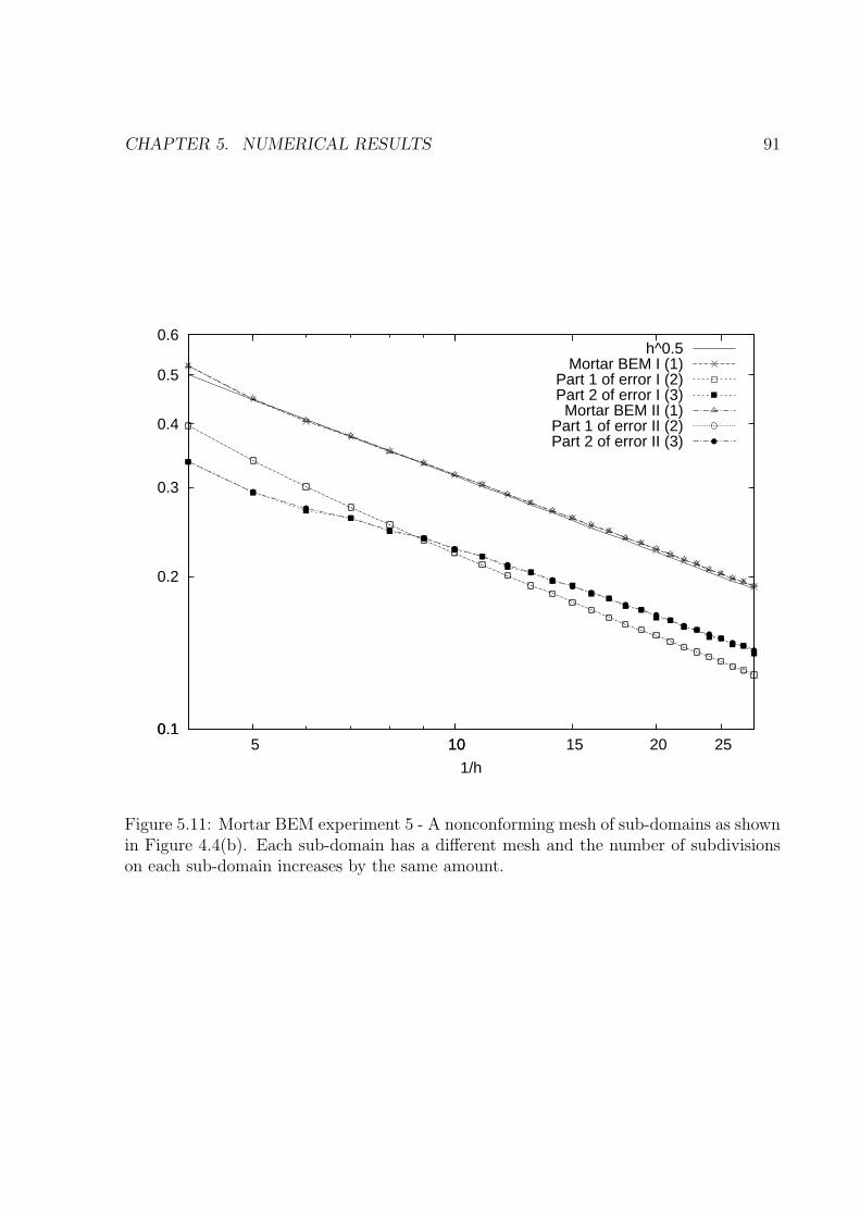
CHAPTER 5. NUMERICAL RESULTS 91
0.1
0.2
0.3
0.4
0.5
0.6
0.1 5 10 15 20 25 10
1/h
h^0.5Mortar BEM I (1)
Part 1 of error I (2)Part 2 of error I (3)
Mortar BEM II (1)Part 1 of error II (2)Part 2 of error II (3)
Figure 5.11: Mortar BEM experiment 5 - A nonconforming mesh of sub-domains as shownin Figure 4.4(b). Each sub-domain has a different mesh and the number of subdivisionson each sub-domain increases by the same amount.
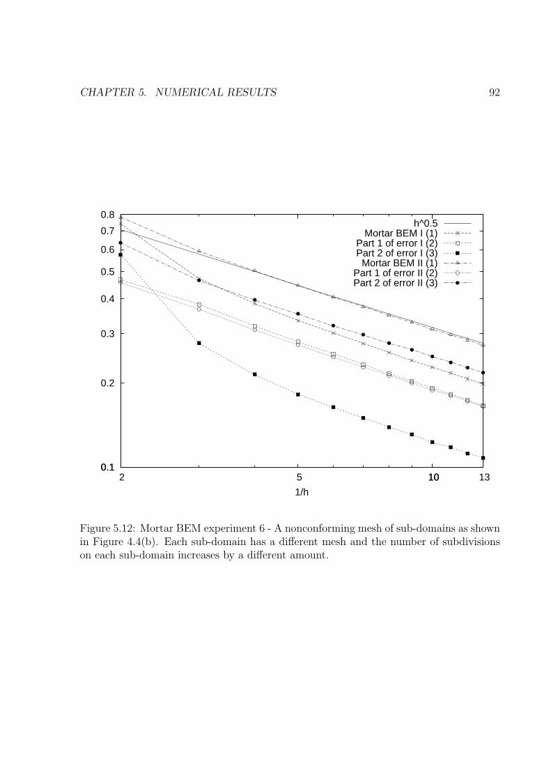
CHAPTER 5. NUMERICAL RESULTS 92
0.1
0.2
0.3
0.4
0.5
0.6
0.7
0.8
0.1 2 5 10 13 10
1/h
h^0.5Mortar BEM I (1)
Part 1 of error I (2)Part 2 of error I (3)
Mortar BEM II (1)Part 1 of error II (2)Part 2 of error II (3)
Figure 5.12: Mortar BEM experiment 6 - A nonconforming mesh of sub-domains as shownin Figure 4.4(b). Each sub-domain has a different mesh and the number of subdivisionson each sub-domain increases by a different amount.
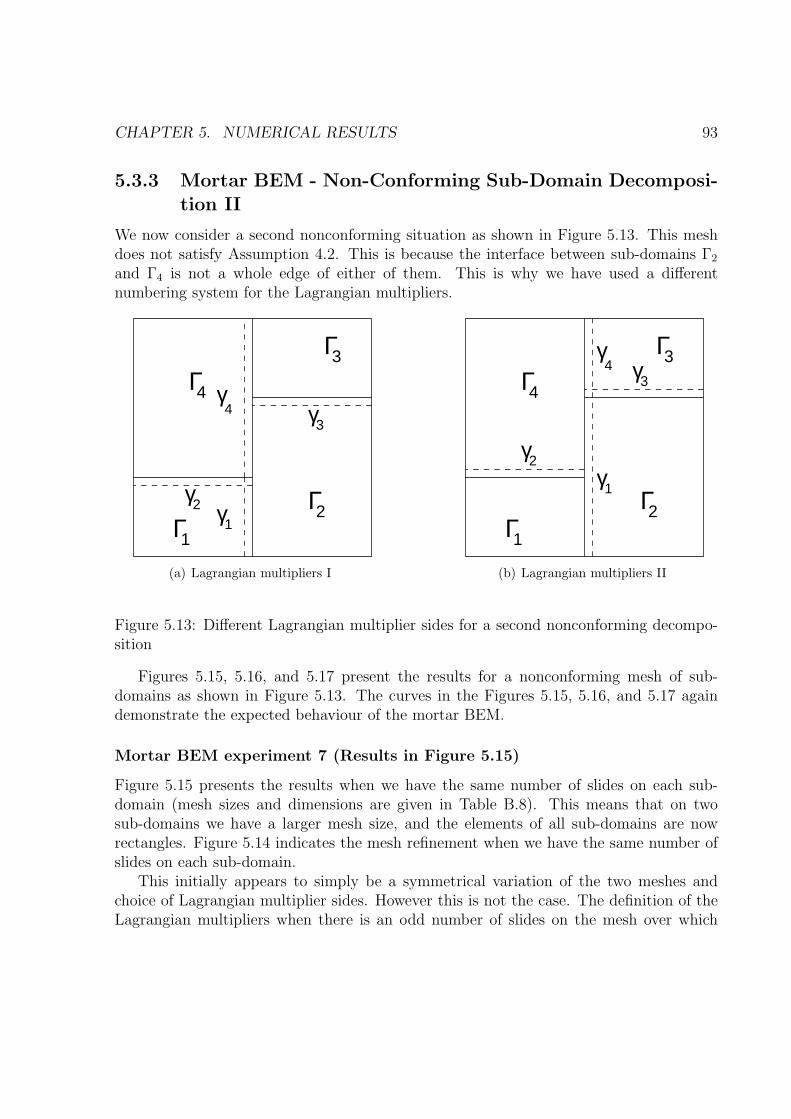
CHAPTER 5. NUMERICAL RESULTS 93
5.3.3 Mortar BEM - Non-Conforming Sub-Domain Decomposi-tion II
We now consider a second nonconforming situation as shown in Figure 5.13. This meshdoes not satisfy Assumption 4.2. This is because the interface between sub-domains Γ2
and Γ4 is not a whole edge of either of them. This is why we have used a differentnumbering system for the Lagrangian multipliers.
Γ
Γ2
4
Γ1
γγ
Γ3
γγ4
3
12
(a) Lagrangian multipliers I
Γ
Γ2
4
Γ1
Γ3γ3
γ1
γ2
γ4
(b) Lagrangian multipliers II
Figure 5.13: Different Lagrangian multiplier sides for a second nonconforming decompo-sition
Figures 5.15, 5.16, and 5.17 present the results for a nonconforming mesh of sub-domains as shown in Figure 5.13. The curves in the Figures 5.15, 5.16, and 5.17 againdemonstrate the expected behaviour of the mortar BEM.
Mortar BEM experiment 7 (Results in Figure 5.15)
Figure 5.15 presents the results when we have the same number of slides on each sub-domain (mesh sizes and dimensions are given in Table B.8). This means that on twosub-domains we have a larger mesh size, and the elements of all sub-domains are nowrectangles. Figure 5.14 indicates the mesh refinement when we have the same number ofslides on each sub-domain.
This initially appears to simply be a symmetrical variation of the two meshes andchoice of Lagrangian multiplier sides. However this is not the case. The definition of theLagrangian multipliers when there is an odd number of slides on the mesh over which
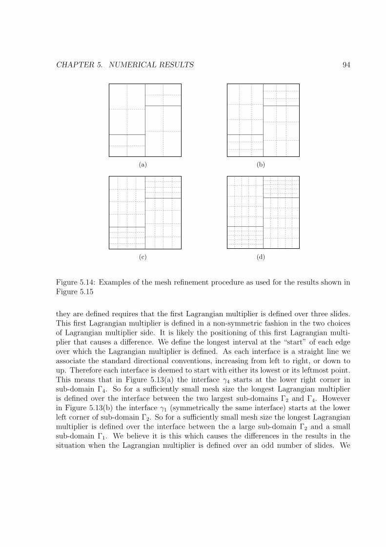
CHAPTER 5. NUMERICAL RESULTS 94
(a) (b)
(c) (d)
Figure 5.14: Examples of the mesh refinement procedure as used for the results shown inFigure 5.15
they are defined requires that the first Lagrangian multiplier is defined over three slides.This first Lagrangian multiplier is defined in a non-symmetric fashion in the two choicesof Lagrangian multiplier side. It is likely the positioning of this first Lagrangian multi-plier that causes a difference. We define the longest interval at the “start” of each edgeover which the Lagrangian multiplier is defined. As each interface is a straight line weassociate the standard directional conventions, increasing from left to right, or down toup. Therefore each interface is deemed to start with either its lowest or its leftmost point.This means that in Figure 5.13(a) the interface γ4 starts at the lower right corner insub-domain Γ4. So for a sufficiently small mesh size the longest Lagrangian multiplieris defined over the interface between the two largest sub-domains Γ2 and Γ4. Howeverin Figure 5.13(b) the interface γ1 (symmetrically the same interface) starts at the lowerleft corner of sub-domain Γ2. So for a sufficiently small mesh size the longest Lagrangianmultiplier is defined over the interface between the a large sub-domain Γ2 and a smallsub-domain Γ1. We believe it is this which causes the differences in the results in thesituation when the Lagrangian multiplier is defined over an odd number of slides. We
CHAPTER 5. NUMERICAL RESULTS 95
note that when there is an even number of slides we simply have a symmetric variationin the definition of the Lagrangian multiplier space.
Mortar BEM experiment 8 (Results in Figure 5.16)
Figure 5.16 presents the result when we start with a different number of slides on eachsub-domain and the increase the number of slides on each sub-domain by one at eachiteration (mesh sizes and dimensions are given in Table B.9). We again see the jumps inthe curves (3) having a large impact on the total error. The differences in the two curves(3) is likely caused by our choice of Lagrangian multiplier side.
Mortar BEM Experiment 9 (Results in Figure 5.17)
Figure 5.17 presents the results when we start with a different number of slides on each sub-domain and then increase the number of slides on each sub-domain by a different numberon each sub-domain (mesh sizes and dimensions are given in Table B.10). If we examinethe sizes of the Lagrangian multiplier spaces in experiment I and experiment II (MkI andMkII in Table B.10 respectively) we see that the choice of Lagrangian multipliers shownin Figure 5.13(a) gives a larger (dimension-wise) Lagrangian multiplier space than thechoice shown in Figure 5.13(b). This is most likely the cause of the differences betweenthe curves (3) in Figure 5.17.
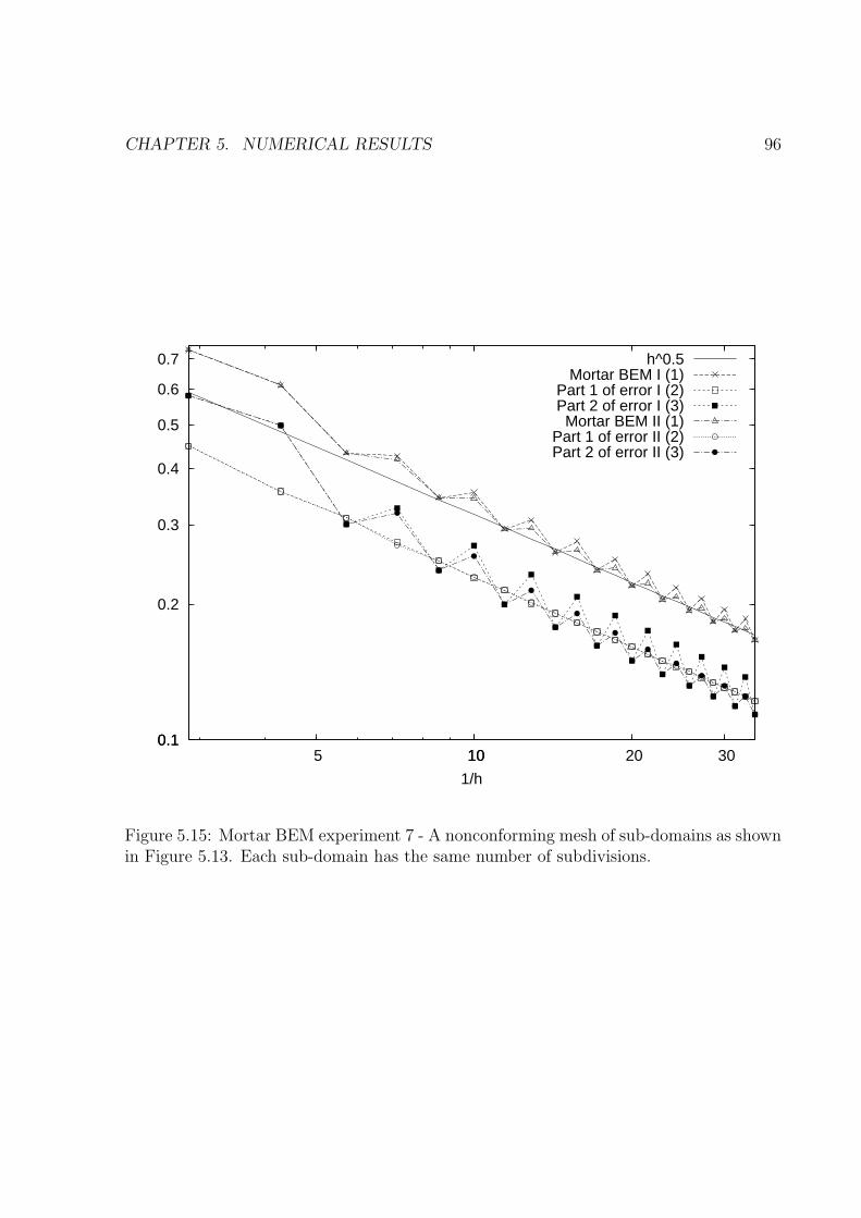
CHAPTER 5. NUMERICAL RESULTS 96
0.1
0.2
0.3
0.4
0.5
0.6
0.7
0.1 5 10 20 30 10
1/h
h^0.5Mortar BEM I (1)
Part 1 of error I (2)Part 2 of error I (3)
Mortar BEM II (1)Part 1 of error II (2)Part 2 of error II (3)
Figure 5.15: Mortar BEM experiment 7 - A nonconforming mesh of sub-domains as shownin Figure 5.13. Each sub-domain has the same number of subdivisions.

CHAPTER 5. NUMERICAL RESULTS 97
0.1
0.2
0.3
0.4
0.5
0.6
0.7
0.1 5 10 20 30 10
1/h
h^0.5Mortar BEM I (1)
Part 1 of error I (2)Part 2 of error I (3)
Mortar BEM II (1)Part 1 of error II (2)Part 2 of error II (3)
Figure 5.16: Mortar BEM experiment 8 - A nonconforming mesh of sub-domains as shownin Figure 5.13. Each sub-domain has a different mesh and the number of subdivisions oneach sub-domain increases by the same amount.
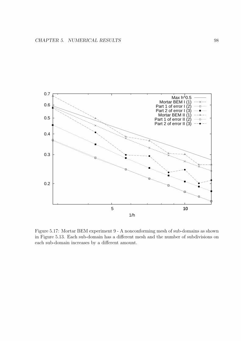
CHAPTER 5. NUMERICAL RESULTS 98
0.2
0.3
0.4
0.5
0.6
0.7
5 10 10
1/h
Max h^0.5Mortar BEM I (1)
Part 1 of error I (2)Part 2 of error I (3)
Mortar BEM II (1)Part 1 of error II (2)Part 2 of error II (3)
Figure 5.17: Mortar BEM experiment 9 - A nonconforming mesh of sub-domains as shownin Figure 5.13. Each sub-domain has a different mesh and the number of subdivisions oneach sub-domain increases by a different amount.
Chapter 6
Mortar BEM for Linear Elasticity
In this chapter we shall extend the results of the mortar BEM from the case of the Lapla-cian to linear elasticity (the Lame system). We first examine the background and settingof the three dimensional Neumann problem in linear elasticity. We then examine themodel problem and discuss the derivation of the model problem. As in the previous chap-ters we require an integration by parts formula to switch from the hypersingular integralequation to an alternative formulation involving weakly singular integrals and present uswith the relevant boundary terms which can be used to define a Lagrangian multiplier.Once we have specified the formulation of the mortar method for linear elasticity we moveonto the analysis. We examine results on the existence and uniqueness of the solution tothe proposed scheme and we examine an error estimate.
Notations
In this section we shall use different notation to that used previously. We are going tobe dealing with functions which are vectors, e.g. φ = (φ1, φ2, φ3), where the subscriptindicates the component of the vector and not the restriction to a sub-domain as previouslyused. We shall use the notation φi|Γj
to indicate the restriction of the ith component ofthe vector φ to the sub-domain Γj.
6.1 Background
6.1.1 Linear Elasticity
We consider the three dimensional Neumann crack problem in linear elasticity. First werecall some notions of linear elasticity from [27] and [37]. We follow the formulation of theproblem as described in [52]. Let the crack surface be denoted by Γ (a plane open surface
99
CHAPTER 6. MORTAR BEM FOR LINEAR ELASTICITY 100
with polygonal boundary). The problem under consideration is for the displacement fieldu of a homogeneous, isotropic elastic material Ω := IR3 \ Γ.
We let u(x) = (u1(x), u2(x), u3(x))T be the displacement vector for x ∈ IR3 where
x = (x1, x2, x3)T and σij(u) be the stress field corresponding to the displacement vector
u. The stress-displacement relationships for an isotropic elastic material are
σij(u) = λδij divu+ 2µǫij, 1 ≤ i, j ≤ 3, (6.1)
where λ and µ are the Lame constants and δij is the Kronecker delta. We assume thatµ > 0 and λ > 2
3µ. The strain tensor ǫij in terms of displacements in (6.1) is given by
ǫij(u) =1
2
(∂ui∂xj
+∂uj∂xi
), 1 ≤ i, j ≤ 3.
For x ∈ IR3 and an arbitrary unit vector n(x) = (n1(x), n2(x), n3(x))T the matrix
differential operator T (∂x,n(x)) is called the stress operator and is defined by
T (∂x,n(x)) = (Tij(∂x,n(x)))3×3, (6.2)
with
Tij(∂x,n(x)) = λni(x)∂
∂xj+ µnj(x)
∂
∂xi+ µδij
∂
∂n(x), 1 ≤ i, j ≤ 3. (6.3)
T (∂x,n(x)) denotes the stress at the point x along the direction n(x) in terms of thedisplacement u(x).
The equilibrium equations without boundary force in elastostatics are
3∑
j=1
∂σij(u)
∂xj= 0, i = 1, 2, 3,
orµ∆u+ (λ+ µ) grad div u = 0, (6.4)
in terms of displacements.We consider the Neumann problem:
µ∆u+ (λ+ µ) grad div u = 0, in Ω
T (∂x,n(x))u = g, on ∂Ω = Γ, (6.5)
where n(x) denotes the outward unit normal on Γ and g = (g1(x), g2(x), g3(x))T is a
vector valued function on the crack surface Γ satisfying∫
Γ
g(x) dS = 0 and
∫
Γ
x× g(x) dS = 0.
CHAPTER 6. MORTAR BEM FOR LINEAR ELASTICITY 101
Under this condition the Neumann problem has a unique solution up to rigid body mo-tions. The rigid body motions are the functions χ ∈ R where
R = span
100
,
010
,
001
,
−x2
x1
0
,
0−x3
x2
,
x3
0−x1
. (6.6)
The rigid body motions can be equivalently defined as the span of the six functionsχj : Γ → IR3 (1 ≤ j ≤ 6) defined by
χl = el and χl+3 = el × x for x ∈ Γ and 1 ≤ l ≤ 3,
where el is the lth column of the 3 × 3 identity matrix. For our crack problems weneed (as in (2.6)) some additional conditions to guarantee the uniqueness of our integralformulation. We require the radiation conditions:
u(x) = o(1) and∂
∂xju(x) = o
(1
|x|
)as |x| → ∞.
We note that the boundary condition in (6.5)
T (∂x,n(x))u = g, on ∂Ω = Γ,
can be equivalently expressed in terms of vectors as
T (∂x,n(x))(u) := λ divun+ 2µ∂u
∂n+ µn× curlu = g, on ∂Ω = Γ.
This is the notation used in [52].
6.1.2 Model problem
Let U ∗(x − y) denote the fundamental solution matrix of the Navier system (6.4). Wethen have that
U ∗(x− y) ≡ (U∗,1(x− y), U∗,2(x− y), U∗,3(x− y)) ≡ (U∗ij(x− y))3×3, (6.7)
with
U∗ij =
1
8πµ(λ+ 2µ)
(λ+ 3µ)
δij|x− y|
+ (λ+ µ)(xi − yi)(xj − yj)
|x− y|3
. (6.8)
The matrix U ∗(x) is symmetric and every column and row of U ∗(x) satisfy the Naviersystem (6.4) at every point x ∈ IR3, except the origin.
CHAPTER 6. MORTAR BEM FOR LINEAR ELASTICITY 102
We now consider the double-layer potential (for linear elasticity)
u(x) =
∫
Γ
(T (∂y,n(y))U ∗(x− y))Tφ(y) dSy, (6.9)
where n(y) denotes the unit outward normal vector at y ∈ Γ and φ is a vector valuedfunction on Γ to be determined. As in Theorem 2.1 φ represents [u], the jump of u overthe crack surface. In (6.9) for a suitable given φ we have that u(x) is a solution of (6.4).The double-layer potential (6.9) can be used to reduce the Neumann problem (6.5) tothe hypersingular boundary integral equation (see [52, Theorem 3.1]) for a given functiong ∈H1/2(Γ)
Wleφ(x) :=
∫
Γ
T (∂x,n(x))(T (∂y,n(y))U ∗(x− y))Tφ(y) dSy = g(x),
x ∈ Γ, φ(x) ∈ H1/2
(Γ). (6.10)
Where we use the notation
Hs(Γ) := (Hs(Γ))3 and Hs(Γ) := (Hs(Γ))3.
The integral equation (6.10) is quite difficult to approximate because of the hypersingularkernel (as it was in the case of the Laplacian in previous chapters). To this end a formu-lation of the hypersingular equation (6.10) using weakly singular integrals was given byNedelec in the following theorem.
Theorem 6.1. [43, Theorem 3]. We have, for Γ a closed surface
〈Wleφ,ψ〉Γ =3∑
i,j=1
∫
Γ
∫
Γ
Gij..(x− y) curlΓ φi(x) · curlΓ ψj(y) dSxdSy
where Gij.. is a tensor of order 4 given by
Gij.. = −curlxcurlyAi.j.(x − y),
CHAPTER 6. MORTAR BEM FOR LINEAR ELASTICITY 103
A being a tensor of order 4 given by
Aijkl(x) =4µ(λ+ µ)
2µ+ λ·
∂4
∂xi∂xj∂xk∂xl
(|x|5
2880π
)
+2λµ
µ+ λ
(∂2
∂xi∂xj
(|x|3
96π
)δkl +
∂2
∂xl∂xk
(|x|3
96π
)δij
)
+ µ
(∂2
∂xi∂xk
(|x|3
96π
)δlj +
∂2
∂xj∂xk
(|x|3
96π
)δli
+∂2
∂xj∂xl
(|x|3
96π
)δki
∂2
∂xi∂xl
(|x|3
96π
)δkj
)
+ µ|x|
8π(δkiδlj + δliδjk) +
2µλ
2µ+ λ
(|x|
8π
)δijδkl.
The given bilinear form is symmetric and elliptic on the space (H1/2(Γ))3/R.
However this formula is extremely complicated, so we shall use an alternative repre-sentation proposed by Han in [27]. As in our earlier situation this is the starting point forour integration by parts formula, and enables us to split the problem up over sub-domains.We have the following mapping property of Wle (from [19]) for an open surface Γ
Wle : H1/2
(Γ) →H−1/2(Γ).
As in the mortar BEM situation of Chapter 4 we need to assume more regularity of thegiven function g than in a standard formulation. In (6.10) we had g ∈H1/2(Γ), howeverfor our mortar method we shall require g ∈ L2(Γ), as was the case in Chapter 4. Astandard boundary element formulation would be to multiply the hypersingular integralequation (6.10) by an appropriate test function and integrate over the boundary to get:
Find φ(x) ∈ H1/2
(Γ) such that
〈Wleφ(x),ψ(x)〉Γ = 〈g(x),ψ(x)〉Γ ∀ψ(x) ∈ H1/2
(Γ). (6.11)
Sub-domain decomposition, meshes and discrete spaces
The same notation and conventions that have been used previously to describe the sub-domain decomposition, meshes and discrete spaces shall be used in this chapter. Fordetails see Chapter 4, in particular for details on sub-domain decomposition see Sec-tion 4.1.2 and for details on meshes and discrete spaces see Section 4.2.1. We shallintroduce two new discrete spaces which are simply product spaces of already definedspaces from Chapter 4:
Xh = (Xh)3 and M k = (Mk)
3.
CHAPTER 6. MORTAR BEM FOR LINEAR ELASTICITY 104
The space Xh was defined in (4.7) and (4.8), and the space Mk was defined in (4.9) and(4.10).
6.1.3 Integration By Parts Formula
As in Chapter 4 we wish to reformulate our hypersingular integral equation in terms ofweakly singular integrals and appropriate derivatives. As before we require an integrationby parts formula for this and importantly we require knowledge of the boundary termwhich this integration by parts introduces for our interface matching condition.
To begin, let us define the differential operator (as in [27]), which are the Gunterderivatives (see e.g. [32]) in matrix form for x ∈ Γ
MΓ(∂x,n(x)) = (MΓ
ij(∂x,n(x)))3×3. (6.12)
The superscript shows restriction of function to the domain and shall be useful laterwhen defining functions over sub-domains (in the same way that we used a subscript inSection 2.3.1). In (6.12) we have the Gunter derivatives
MΓij(∂x,n(x)) = nj(x)
∂
∂xi− ni(x)
∂
∂xj. (6.13)
We can now write the following operators
MΓ11(∂x,n(x)) = MΓ
22(∂x,n(x)) = MΓ33(∂x,n(x)) = 0
MΓ32(∂x,n(x)) = −MΓ
23(∂x,n(x)) =∂
∂SΓ1 (x)
MΓ13(∂x,n(x)) = −MΓ
31(∂x,n(x)) =∂
∂SΓ2 (x)
MΓ21(∂x,n(x)) = −MΓ
12(∂x,n(x)) =∂
∂SΓ3 (x)
.
Where
SΓ1 (x) = (0,−n3(x), n2(x))
T x ∈ Γ
SΓ2 (x) = (n3(x), 0,−n1(x))
T x ∈ Γ
SΓ3 (x) = (−n2(x), n1(x), 0)T x ∈ Γ.
CHAPTER 6. MORTAR BEM FOR LINEAR ELASTICITY 105
We note that MΓ(∂x,n(x)) can be expressed in matrix form as
0 − ∂∂SΓ
3
∂∂SΓ
2∂
∂SΓ3
0 − ∂∂SΓ
1
− ∂∂SΓ
2
∂∂SΓ
10
. (6.14)
Following Han [27] we let φ(x) = (φ1(x), φ2(x), φ3(x))T and
ψ(x) = (ψ1(x), ψ2(x), ψ3(x))T be the traces of u(x) = (u1(x), u2(x), u3(x))
T and v(x) =(v1(x), v2(x), v3(x))
T respectively. We present the following lemma as the proof gives usan indication as to where our boundary term in the integration by parts formula will comefrom.
Lemma 6.2. [27, equation (3.12)] For a closed surface Γ and functionsφ,ψ ∈H1/2(Γ)/R, we have the following identity
〈Wleφ,ψ〉Γ =
∫
Γ
∫
Γ
µ
4π
1
|x− y|
(3∑
k=1
∂ψ(x)
∂SΓk (x)
·∂φ(y)
∂SΓk (y)
)dSydSx
+
∫
Γ
∫
Γ
(MΓ(∂x,n(x))ψ(x))T(µ
2πI
1
|x− y|
−4µ2U ∗(x− y))M
Γ(∂y,n(y))φ(y) dSydSx (6.15)
+
∫
Γ
∫
Γ
µ
4π
3∑
i,j,k=1
(MΓkj(∂x,n(x))ψi(x))
1
|x− y|(MΓ
ki(∂y,n(y))φj(y)) dSydSx.
Proof. We now refer back to the model problem (6.11) and see that this can be expressedas
〈Wleφ,ψ〉Γ = −
∫
Γ
(T (∂x,n(x))u(x)) ·ψ(x)dSx. (6.16)
In the above u can be replaced by the double-layer potential defined in (6.9). The stressoperator defined in (6.2) and (6.3) can be re-expressed as [27, equation (2.12)]
T (∂x,n(x))u(x) =3∑
k=1
∂
∂SΓk (x)
∫
Γ
µ
4π
1
|x− y|
∂φ(y)
∂SΓk (y)
dSy
+ MΓ(∂x,n(x))
∫
Γ
(4µ2U ∗(x− y)
−µ
2πI
1
|x− y|
)M
Γ(∂y,n(y))φ(y)dSy (6.17)
−µ
4π
∫
Γ
[M
Γ(∂x,n(x))1
|x− y|M
Γ(∂y,n(y))
]Tφ(y)dSy.
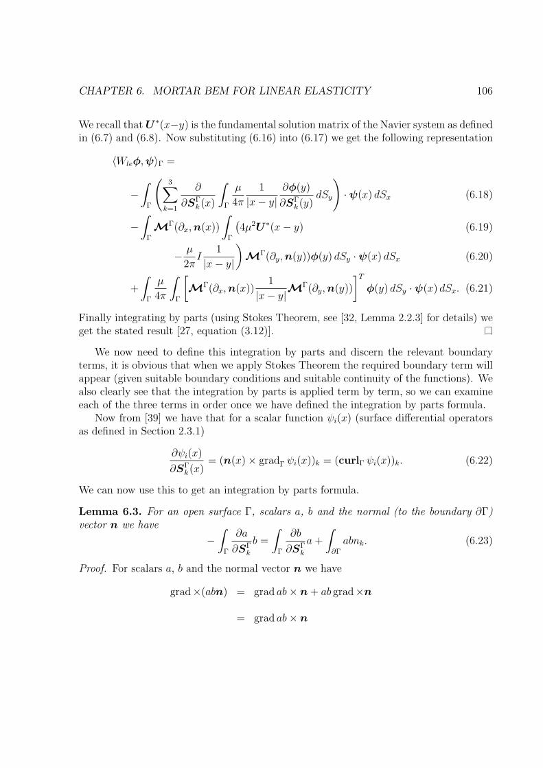
CHAPTER 6. MORTAR BEM FOR LINEAR ELASTICITY 106
We recall thatU ∗(x−y) is the fundamental solution matrix of the Navier system as definedin (6.7) and (6.8). Now substituting (6.16) into (6.17) we get the following representation
〈Wleφ,ψ〉Γ =
−
∫
Γ
(3∑
k=1
∂
∂SΓk (x)
∫
Γ
µ
4π
1
|x− y|
∂φ(y)
∂SΓk (y)
dSy
)·ψ(x) dSx (6.18)
−
∫
Γ
MΓ(∂x,n(x))
∫
Γ
(4µ2U ∗(x− y) (6.19)
−µ
2πI
1
|x− y|
)M
Γ(∂y,n(y))φ(y) dSy ·ψ(x) dSx (6.20)
+
∫
Γ
µ
4π
∫
Γ
[M
Γ(∂x,n(x))1
|x− y|M
Γ(∂y,n(y))
]Tφ(y) dSy ·ψ(x) dSx. (6.21)
Finally integrating by parts (using Stokes Theorem, see [32, Lemma 2.2.3] for details) weget the stated result [27, equation (3.12)].
We now need to define this integration by parts and discern the relevant boundaryterms, it is obvious that when we apply Stokes Theorem the required boundary term willappear (given suitable boundary conditions and suitable continuity of the functions). Wealso clearly see that the integration by parts is applied term by term, so we can examineeach of the three terms in order once we have defined the integration by parts formula.
Now from [39] we have that for a scalar function ψi(x) (surface differential operatorsas defined in Section 2.3.1)
∂ψi(x)
∂SΓk (x)
= (n(x) × gradΓ ψi(x))k = (curlΓ ψi(x))k. (6.22)
We can now use this to get an integration by parts formula.
Lemma 6.3. For an open surface Γ, scalars a, b and the normal (to the boundary ∂Γ)vector n we have
−
∫
Γ
∂a
∂SΓk
b =
∫
Γ
∂b
∂SΓk
a+
∫
∂Γ
abnk. (6.23)
Proof. For scalars a, b and the normal vector n we have
grad×(abn) = grad ab× n+ ab grad×n
= grad ab× n
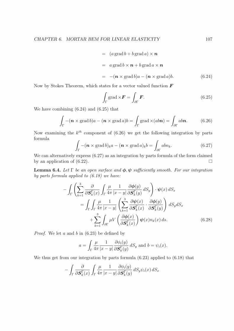
CHAPTER 6. MORTAR BEM FOR LINEAR ELASTICITY 107
= (a grad b+ b grad a) × n
= a grad b× n+ b grad a× n
= −(n× grad b)a− (n× grad a)b. (6.24)
Now by Stokes Theorem, which states for a vector valued function F∫
Γ
grad×F =
∫
∂Γ
F . (6.25)
We have combining (6.24) and (6.25) that∫
Γ
−(n× grad b)a− (n× grad a)b =
∫
Γ
grad×(abn) =
∫
∂Γ
abn. (6.26)
Now examining the kth component of (6.26) we get the following integration by partsformula ∫
Γ
−(n× grad b)ka− (n× grad a)kb =
∫
∂Γ
abnk. (6.27)
We can alternatively express (6.27) as an integration by parts formula of the form claimedby an application of (6.22).
Lemma 6.4. Let Γ be an open surface and φ,ψ sufficiently smooth. For our integrationby parts formula applied to (6.18) we have:
−
∫
Γ
(3∑
k=1
∂
∂SΓk (x)
∫
Γ
µ
4π
1
|x− y|
∂φ(y)
∂SΓk (y)
dSy
)·ψ(x) dSx
=
∫
Γ
∫
Γ
µ
4π
1
|x− y|
(3∑
k=1
∂ψ(x)
∂SΓk (x)
·∂φ(y)
∂SΓk (y)
)dSydSx
+3∑
k=1
∫
∂Γ
µV
(∂φ(x)
∂SΓk (x)
)ψ(x)nk(x) ds. (6.28)
Proof. We let a and b in (6.23) be defined by
a =
∫
Γ
µ
4π
1
|x− y|
∂φi(y)
∂SΓk (y)
dSy and b = ψi(x).
We thus get from our integration by parts formula (6.23) applied to (6.18) that
−
∫
Γ
∂
∂SΓk (x)
∫
Γ
µ
4π
1
|x− y|
∂φi(y)
∂SΓk (y)
dSyψi(x) dSx
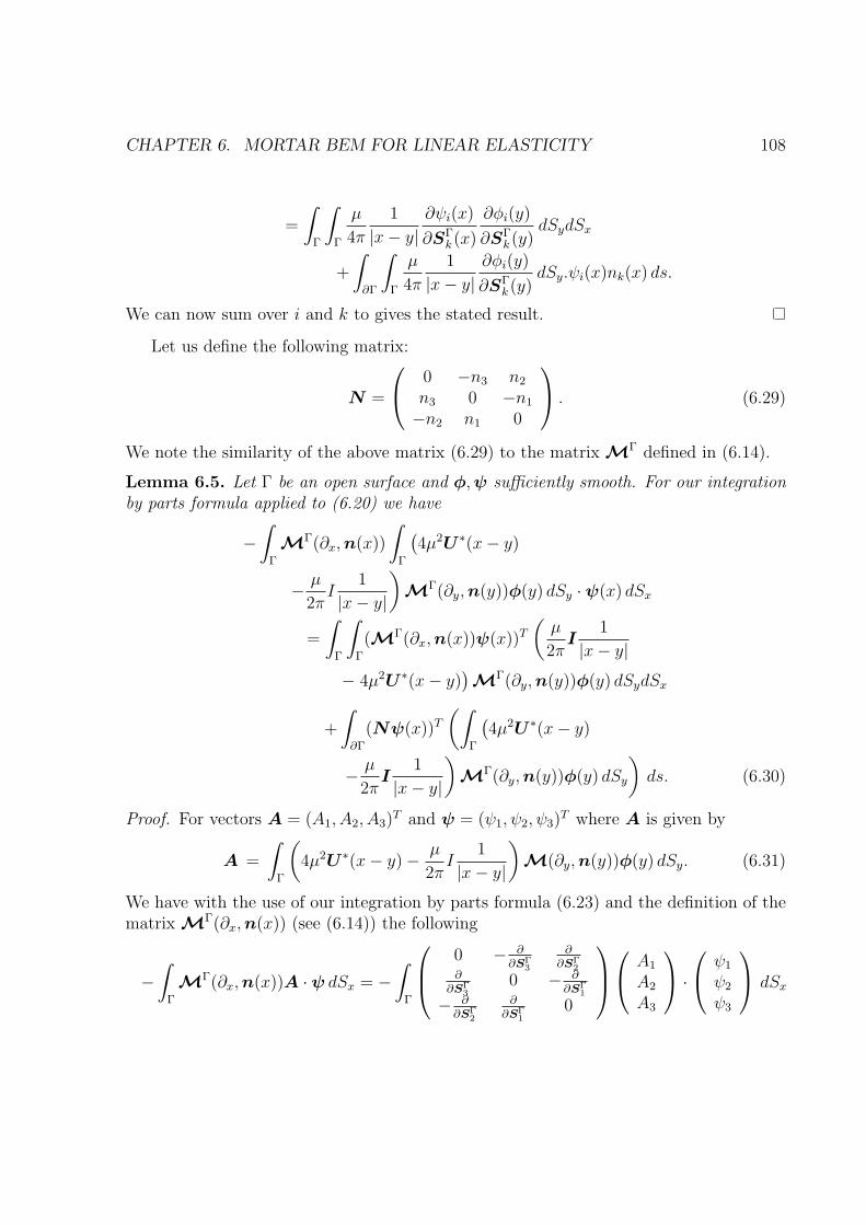
CHAPTER 6. MORTAR BEM FOR LINEAR ELASTICITY 108
=
∫
Γ
∫
Γ
µ
4π
1
|x− y|
∂ψi(x)
∂SΓk (x)
∂φi(y)
∂SΓk (y)
dSydSx
+
∫
∂Γ
∫
Γ
µ
4π
1
|x− y|
∂φi(y)
∂SΓk (y)
dSy.ψi(x)nk(x) ds.
We can now sum over i and k to gives the stated result.
Let us define the following matrix:
N =
0 −n3 n2
n3 0 −n1
−n2 n1 0
. (6.29)
We note the similarity of the above matrix (6.29) to the matrix MΓ defined in (6.14).
Lemma 6.5. Let Γ be an open surface and φ,ψ sufficiently smooth. For our integrationby parts formula applied to (6.20) we have
−
∫
Γ
MΓ(∂x,n(x))
∫
Γ
(4µ2U ∗(x− y)
−µ
2πI
1
|x− y|
)M
Γ(∂y,n(y))φ(y) dSy ·ψ(x) dSx
=
∫
Γ
∫
Γ
(MΓ(∂x,n(x))ψ(x))T(µ
2πI
1
|x− y|
− 4µ2U ∗(x− y))M
Γ(∂y,n(y))φ(y) dSydSx
+
∫
∂Γ
(Nψ(x))T(∫
Γ
(4µ2U ∗(x− y)
−µ
2πI
1
|x− y|
)M
Γ(∂y,n(y))φ(y) dSy
)ds. (6.30)
Proof. For vectors A = (A1, A2, A3)T and ψ = (ψ1, ψ2, ψ3)
T where A is given by
A =
∫
Γ
(4µ2U ∗(x− y) −
µ
2πI
1
|x− y|
)M(∂y,n(y))φ(y) dSy. (6.31)
We have with the use of our integration by parts formula (6.23) and the definition of thematrix M
Γ(∂x,n(x)) (see (6.14)) the following
−
∫
Γ
MΓ(∂x,n(x))A ·ψ dSx = −
∫
Γ
0 − ∂∂SΓ
3
∂∂SΓ
2∂
∂SΓ3
0 − ∂∂SΓ
1
− ∂∂SΓ
2
∂∂SΓ
10
A1
A2
A3
·
ψ1
ψ2
ψ3
dSx
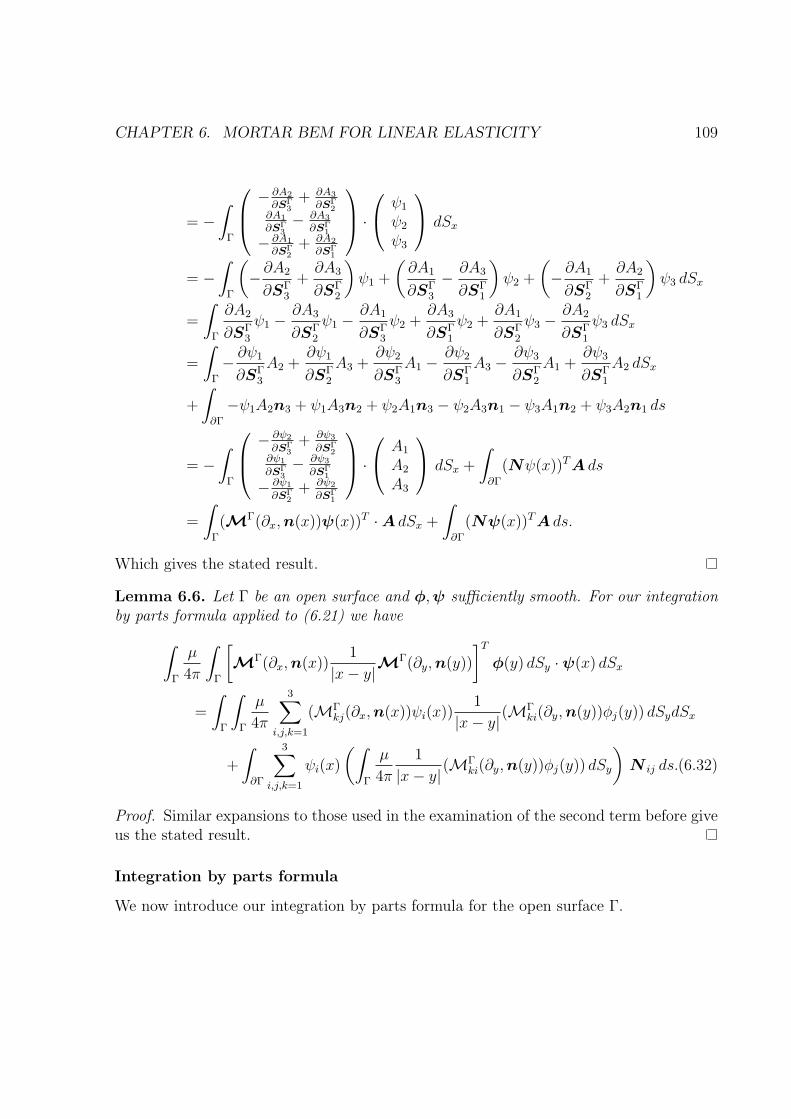
CHAPTER 6. MORTAR BEM FOR LINEAR ELASTICITY 109
= −
∫
Γ
− ∂A2
∂SΓ3
+ ∂A3
∂SΓ2
∂A1
∂SΓ3− ∂A3
∂SΓ1
− ∂A1
∂SΓ2
+ ∂A2
∂SΓ1
·
ψ1
ψ2
ψ3
dSx
= −
∫
Γ
(−∂A2
∂SΓ3
+∂A3
∂SΓ2
)ψ1 +
(∂A1
∂SΓ3
−∂A3
∂SΓ1
)ψ2 +
(−∂A1
∂SΓ2
+∂A2
∂SΓ1
)ψ3 dSx
=
∫
Γ
∂A2
∂SΓ3
ψ1 −∂A3
∂SΓ2
ψ1 −∂A1
∂SΓ3
ψ2 +∂A3
∂SΓ1
ψ2 +∂A1
∂SΓ2
ψ3 −∂A2
∂SΓ1
ψ3 dSx
=
∫
Γ
−∂ψ1
∂SΓ3
A2 +∂ψ1
∂SΓ2
A3 +∂ψ2
∂SΓ3
A1 −∂ψ2
∂SΓ1
A3 −∂ψ3
∂SΓ2
A1 +∂ψ3
∂SΓ1
A2 dSx
+
∫
∂Γ
−ψ1A2n3 + ψ1A3n2 + ψ2A1n3 − ψ2A3n1 − ψ3A1n2 + ψ3A2n1 ds
= −
∫
Γ
− ∂ψ2
∂SΓ3
+ ∂ψ3
∂SΓ2
∂ψ1
∂SΓ3− ∂ψ3
∂SΓ1
− ∂ψ1
∂SΓ2
+ ∂ψ2
∂SΓ1
·
A1
A2
A3
dSx +
∫
∂Γ
(Nψ(x))TA ds
=
∫
Γ
(MΓ(∂x,n(x))ψ(x))T ·A dSx +
∫
∂Γ
(Nψ(x))TA ds.
Which gives the stated result.
Lemma 6.6. Let Γ be an open surface and φ,ψ sufficiently smooth. For our integrationby parts formula applied to (6.21) we have
∫
Γ
µ
4π
∫
Γ
[M
Γ(∂x,n(x))1
|x− y|M
Γ(∂y,n(y))
]Tφ(y) dSy ·ψ(x) dSx
=
∫
Γ
∫
Γ
µ
4π
3∑
i,j,k=1
(MΓkj(∂x,n(x))ψi(x))
1
|x− y|(MΓ
ki(∂y,n(y))φj(y)) dSydSx
+
∫
∂Γ
3∑
i,j,k=1
ψi(x)
(∫
Γ
µ
4π
1
|x− y|(MΓ
ki(∂y,n(y))φj(y)) dSy
)N ij ds.(6.32)
Proof. Similar expansions to those used in the examination of the second term before giveus the stated result.
Integration by parts formula
We now introduce our integration by parts formula for the open surface Γ.
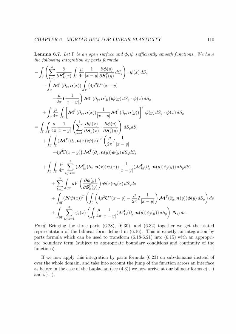
CHAPTER 6. MORTAR BEM FOR LINEAR ELASTICITY 110
Lemma 6.7. Let Γ be an open surface and φ,ψ sufficiently smooth functions. We havethe following integration by parts formula
−
∫
Γ
(3∑
k=1
∂
∂SΓk (x)
∫
Γ
µ
4π
1
|x− y|
∂φ(y)
∂SΓk (y)
dSy
)·ψ(x) dSx
−
∫
Γ
MΓ(∂x,n(x))
∫
Γ
(4µ2U ∗(x− y)
−µ
2πI
1
|x− y|
)M
Γ(∂y,n(y))φ(y) dSy ·ψ(x) dSx
+
∫
Γ
µ
4π
∫
Γ
[M
Γ(∂x,n(x))1
|x− y|M
Γ(∂y,n(y))
]Tφ(y) dSy ·ψ(x) dSx
=
∫
Γ
∫
Γ
µ
4π
1
|x− y|
(3∑
k=1
∂ψ(x)
∂SΓk (x)
·∂φ(y)
∂SΓk (y)
)dSydSx
+
∫
Γ
∫
Γ
(MΓ(∂x,n(x))ψ(x))T(µ
2πI
1
|x− y|
−4µ2Γ(x− y))M
Γ(∂y,n(y))φ(y) dSydSx
+
∫
Γ
∫
Γ
µ
4π
3∑
i,j,k=1
(MΓkj(∂x,n(x))ψi(x))
1
|x− y|(MΓ
ki(∂y,n(y))φj(y)) dSydSx
+3∑
k=1
∫
∂Γ
µV
(∂φ(y)
∂SΓk (y)
)ψ(x)nk(x) dSyds
+
∫
∂Γ
(Nψ(x))T(∫
Γ
(4µ2U ∗(x− y) −
µ
2πI
1
|x− y|
)M
Γ(∂y,n(y))φ(y) dSy
)ds
+
∫
∂Γ
3∑
i,j,k=1
ψi(x)
(∫
Γ
µ
4π
1
|x− y|(MΓ
ki(∂y,n(y))φj(y)) dSy
)N ij ds.
Proof. Bringing the three parts (6.28), (6.30), and (6.32) together we get the statedrepresentation of the bilinear form defined in (6.16). This is exactly an integration byparts formula which can be used to transform (6.18-6.21) into (6.15) with an appropri-ate boundary term (subject to appropriate boundary conditions and continuity of thefunctions).
If we now apply this integration by parts formula (6.23) on sub-domains instead ofover the whole domain, and take into account the jump of the function across an interfaceas before in the case of the Laplacian (see (4.3)) we now arrive at our bilinear forms a(·, ·)and b(·, ·).
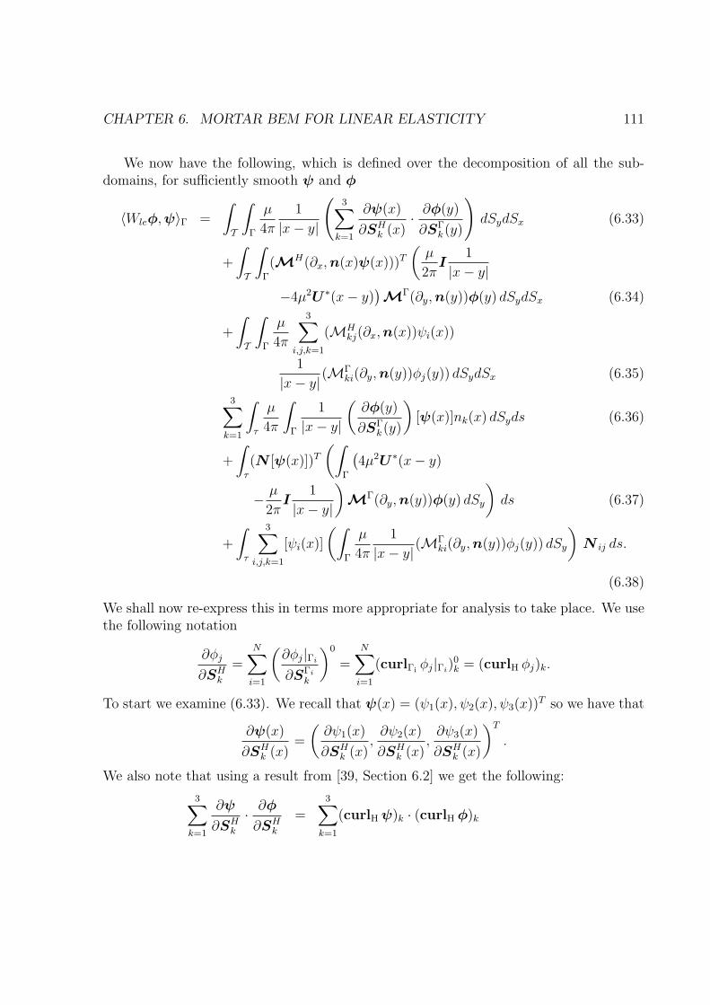
CHAPTER 6. MORTAR BEM FOR LINEAR ELASTICITY 111
We now have the following, which is defined over the decomposition of all the sub-domains, for sufficiently smooth ψ and φ
〈Wleφ,ψ〉Γ =
∫
T
∫
Γ
µ
4π
1
|x− y|
(3∑
k=1
∂ψ(x)
∂SHk (x)·∂φ(y)
∂SΓk (y)
)dSydSx (6.33)
+
∫
T
∫
Γ
(MH(∂x,n(x)ψ(x)))T(µ
2πI
1
|x− y|
−4µ2U ∗(x− y))M
Γ(∂y,n(y))φ(y) dSydSx (6.34)
+
∫
T
∫
Γ
µ
4π
3∑
i,j,k=1
(MHkj(∂x,n(x))ψi(x))
1
|x− y|(MΓ
ki(∂y,n(y))φj(y)) dSydSx (6.35)
3∑
k=1
∫
τ
µ
4π
∫
Γ
1
|x− y|
(∂φ(y)
∂SΓk (y)
)[ψ(x)]nk(x) dSyds (6.36)
+
∫
τ
(N [ψ(x)])T(∫
Γ
(4µ2U ∗(x− y)
−µ
2πI
1
|x− y|
)M
Γ(∂y,n(y))φ(y) dSy
)ds (6.37)
+
∫
τ
3∑
i,j,k=1
[ψi(x)]
(∫
Γ
µ
4π
1
|x− y|(MΓ
ki(∂y,n(y))φj(y)) dSy
)N ij ds.
(6.38)
We shall now re-express this in terms more appropriate for analysis to take place. We usethe following notation
∂φj
∂SHk=
N∑
i=1
(∂φj|Γi
∂SΓik
)0
=N∑
i=1
(curlΓiφj|Γi
)0k = (curlH φj)k.
To start we examine (6.33). We recall that ψ(x) = (ψ1(x), ψ2(x), ψ3(x))T so we have that
∂ψ(x)
∂SHk (x)=
(∂ψ1(x)
∂SHk (x),∂ψ2(x)
∂SHk (x),∂ψ3(x)
∂SHk (x)
)T.
We also note that using a result from [39, Section 6.2] we get the following:
3∑
k=1
∂ψ
∂SHk·∂φ
∂SHk=
3∑
k=1
(curlHψ)k · (curlHφ)k
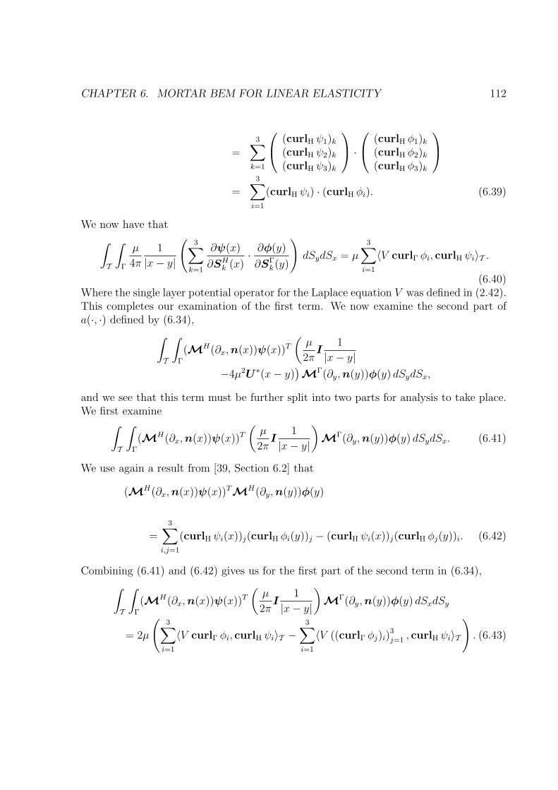
CHAPTER 6. MORTAR BEM FOR LINEAR ELASTICITY 112
=3∑
k=1
(curlH ψ1)k(curlH ψ2)k(curlH ψ3)k
·
(curlH φ1)k(curlH φ2)k(curlH φ3)k
=3∑
i=1
(curlH ψi) · (curlH φi). (6.39)
We now have that
∫
T
∫
Γ
µ
4π
1
|x− y|
(3∑
k=1
∂ψ(x)
∂SHk (x)·∂φ(y)
∂SΓk (y)
)dSydSx = µ
3∑
i=1
〈V curlΓ φi, curlH ψi〉T .
(6.40)Where the single layer potential operator for the Laplace equation V was defined in (2.42).This completes our examination of the first term. We now examine the second part ofa(·, ·) defined by (6.34),
∫
T
∫
Γ
(MH(∂x,n(x))ψ(x))T(µ
2πI
1
|x− y|
−4µ2U ∗(x− y))M
Γ(∂y,n(y))φ(y) dSydSx,
and we see that this term must be further split into two parts for analysis to take place.We first examine
∫
T
∫
Γ
(MH(∂x,n(x))ψ(x))T(µ
2πI
1
|x− y|
)M
Γ(∂y,n(y))φ(y) dSydSx. (6.41)
We use again a result from [39, Section 6.2] that
(MH(∂x,n(x))ψ(x))TMH(∂y,n(y))φ(y)
=3∑
i,j=1
(curlH ψi(x))j(curlH φi(y))j − (curlH ψi(x))j(curlH φj(y))i. (6.42)
Combining (6.41) and (6.42) gives us for the first part of the second term in (6.34),
∫
T
∫
Γ
(MH(∂x,n(x))ψ(x))T(µ
2πI
1
|x− y|
)M
Γ(∂y,n(y))φ(y) dSxdSy
= 2µ
(3∑
i=1
〈V curlΓ φi, curlH ψi〉T −3∑
i=1
〈V ((curlΓ φj)i)3j=1 , curlH ψi〉T
). (6.43)
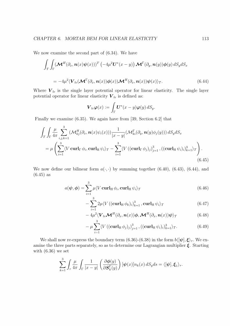
CHAPTER 6. MORTAR BEM FOR LINEAR ELASTICITY 113
We now examine the second part of (6.34). We have∫
T
∫
Γ
(MH(∂x,n(x)ψ(x)))T(−4µ2U ∗(x− y)
)M
Γ(∂y,n(y))φ(y) dSydSx
= −4µ2〈V le(MΓ(∂x,n(x))φ(x))MH(∂x,n(x))ψ(x)〉T . (6.44)
Where V le is the single layer potential operator for linear elasticity. The single layerpotential operator for linear elasticity V le is defined as:
V leϕ(x) :=
∫
Γ
U ∗(x− y)ϕ(y) dSy.
Finally we examine (6.35). We again have from [39, Section 6.2] that
∫
T
∫
Γ
µ
4π
3∑
i,j,k=1
(MHkj(∂x,n(x)ψi(x)))
1
|x− y|(MΓ
ki(∂y,n(y)φj(y))) dSydSx
= µ
(3∑
i=1
〈V curlΓ φi, curlH ψi〉T −3∑
i=1
〈V ((curlΓ φj)j)3j=1 , ((curlH ψi)i)
3k=1〉T
).
(6.45)
We now define our bilinear form a(·, ·) by summing together (6.40), (6.43), (6.44), and(6.45) as
a(ψ,φ) =3∑
i=1
µ〈V curlH φi, curlH ψi〉T (6.46)
−3∑
i=1
2µ〈V ((curlH φk)i)3k=1 , curlH ψi〉T (6.47)
− 4µ2〈V leMH(∂x,n(x))φ,MH(∂x,n(x))ψ〉T (6.48)
− µ3∑
i=1
〈V ((curlH φj)j)3j=1 , ((curlH ψi)i)
3k=1〉T . (6.49)
We shall now re-express the boundary term (6.36)-(6.38) in the form b〈[ψ], ξ〉τ . We ex-amine the three parts separately, so as to determine our Lagrangian multiplier ξ. Startingwith (6.36) we set
3∑
k=1
∫
τ
µ
4π
∫
Γ
1
|x− y|
(∂φ(y)
∂SΓk (y)
)[ψ(x)]nk(x) dSyds = 〈[ψ], ξ1〉τ .
CHAPTER 6. MORTAR BEM FOR LINEAR ELASTICITY 114
This gives us that
ξ1|γl=
3∑
k=1
µ
(V
(∂φ(y)
∂SΓk (y)
)) ∣∣∣γl
nk(x). (6.50)
Alternatively we can express ξ1 as ξ1 = (n(x) · (V curlΓφi)|γl)3i=1. We now examine the
second part (6.37) of the boundary term
∫
τ
(N [ψ(x)])T(∫
Γ
(4µ2U ∗(x− y)
−µ
2πI
1
|x− y|
)M
Γ(∂y,n(y))φ(y) dSy
)ds = 〈[ψ], ξ2〉τ .
Now since (N [ψ(x)])T = ([ψ(x)])TNT , we have that
ξ2|γl= NT
((4µ2Vle − 2µV
)M
Γ(∂y,n(y))φ(y))|γl. (6.51)
Finally we examine the third part (6.38) of the bilinear form b(·, ·)
∫
τ
3∑
i,j,k=1
[ψi(x)]
(∫
Γ
µ
4π
1
|x− y|(MΓ
ki(∂y,n(y))φj(y)) dSy
)N ij ds = 〈[ψ], ξ3〉τ .
This gives us
ξ3|γl=
(3∑
k=1
µ((V (MΓ
ki(∂y,n(y))φj(y))∣∣γl
)3
j=1· (N ij)
3j=1
)3
i=1
. (6.52)
We thus have by (6.50), (6.51), and (6.52) our boundary term b(·, ·) associated with (6.33)to (6.35) is given by
b(ψ, ξ) = 〈[ψ], ξ〉τ =L∑
l=1
〈[ψ], ξ〉γlwhere ξ =
3∑
i=1
ξi. (6.53)
We now have our standard mixed formulation as in the previous situations, we can thusproceed as before to prove existence and uniqueness of a solution and an error estimate.Our mixed formulation of the Mortar BEM for linear elasticity is thus: Find φh ∈ Xh
and ξk ∈M k such that
a(φh,ψ) + b(ψ, ξk) = F (ψ) ∀ψ ∈Xh
b(φh,η) = 0 ∀η ∈M k.(6.54)
CHAPTER 6. MORTAR BEM FOR LINEAR ELASTICITY 115
For the bilinear forms a(·, ·) defined in (6.49)-(6.49) and b(·, ·) defined in (6.53) . As inthe previous chapters we have that this scheme is equivalent to: Find φh ∈ V h such that
a(φh,ψ) = F (ψ) ∀ψ ∈ V h. (6.55)
Where the constrained space V h is defined as
V h = ψ ∈Xh : b(ψ,η) = 0 ∀η ∈M k . (6.56)
6.2 Technical Results and Proof of the Main Result
In this section we present the analysis which leads to our main error result. As in theprevious chapters continuity and ellipticity of the bilinear form a(·, ·) are essential for theerror analysis of the problem described in (6.54). We first present some results relatingto the continuity of a(·, ·) which shall be used to show that associated with a functionthat satisfies our model problem is a Lagrangian multiplier that is well defined despitethe absence of an appropriate trace theorem.
Preliminary remarks
We first examine some bounds for our bilinear form a(·, ·) defined in (6.46)-(6.49).
Lemma 6.8. For the first part (6.46) of the bilinear form a(·, ·) we have
µ
3∑
i=1
〈V curlH φi, curlH ψi〉T
. µ
(3∑
i=1
‖ curlH φi‖H−1/2t (T )
)(3∑
i=1
‖ curlH ψi‖H−1/2t (T )
). (6.57)
Proof. As in the case of the Laplacian we have by the continuity of V : H−1/2
t (Γ) →
H1/2t (Γ) (by [19]) we have
µ
3∑
i=1
〈V curlH φi, curlH ψi〉T
. µ3∑
i=1
‖ curlH ψi‖H−1/2t (T )
‖ curlH φi‖H−1/2t (T )
. µ
(3∑
i=1
‖ curlH φi‖H−1/2t (T )
)(3∑
i=1
‖ curlH ψi‖H−1/2t (T )
).
Which is the stated result.

CHAPTER 6. MORTAR BEM FOR LINEAR ELASTICITY 116
Lemma 6.9. For the second part (6.47) of the bilinear form a(·, ·) we have
|3∑
i=1
2µ〈V ((curlH φj)i)3j=1 , curlH ψi〉T |
. 2µ
(3∑
i=1
‖ curlH φi‖H−1/2t (T )
)(3∑
i=1
‖ curlH ψi‖H−1/2t (T )
). (6.58)
Proof. Now by the continuity of V : H−1/2
t (Γ) →H1/2t (Γ) (by [19]) we have
|3∑
i=1
2µ〈V ((curlH φj)i)3j=1 , curlH ψi〉T |
. 2µ3∑
i=1
‖ ((curlH φj)i)3j=1 ‖H−1/2
t (T )‖ curlH ψi‖H−1/2
t (T )
. 2µ
(3∑
i=1
‖ ((curlH φj)i)3j=1 ‖H−1/2
t (T )
)(3∑
i=1
‖ curlH ψi‖H−1/2t (T )
)
. 2µ
(3∑
i=1
‖ curlH φi‖H−1/2t (T )
)(3∑
i=1
‖ curlH ψi‖H−1/2t (T )
,
)(6.59)
by a simple rearrangement of terms. The stated result then follows immediately.
Lemma 6.10. For the third part (6.48) of the bilinear form a(·, ·) we have
|4µ2〈V le(MH(∂x,n(x))φ(x))MH(∂x,n(x))ψ(x)〉T |
. 4µ2
(3∑
i=1
‖ curlH φi‖H−1/2t (T )
)(3∑
i=1
‖ curlH ψi‖H−1/2t (T )
). (6.60)
Proof. From [19] we have the continuity of Vle : H−1/2
(Γ) →H1/2(Γ) which gives us that
|4µ2〈V le(MH(∂x,n(x))φ(x))MH(∂x,n(x)ψ(x))〉T |
. 4µ2‖MH(∂x,n(x))φ(x)‖2
H−1/2
(T )‖MH(∂x,n(x))φ(x)‖2
H−1/2
(T ). (6.61)
CHAPTER 6. MORTAR BEM FOR LINEAR ELASTICITY 117
The norm in (6.61) can be expressed as
‖MH(∂x,n(x))φ(x)‖2
H−1/2
(T )=
‖ − (curlH φ2)3 + (curlH φ3)2‖2H−1/2(T )
+‖(curlH φ1)3 − (curlH φ3)1‖2H−1/2(T )
+‖ − (curlH φ1)2 + (curlH φ2)1‖2H−1/2(T )
. (6.62)
We can trivially bound (6.62) by the triangle inequality and adding in the extra terms inthe following way:
‖MH(∂x,n(x))φ(x)‖2
H−1/2
(T ).
3∑
i=1
‖ curlH φi‖2
H−1/2
(T ).
3∑
i=1
‖ curlH φi‖2
H−1/2t (T )
.
The stated result then follows immediately.
Lemma 6.11. For the fourth part of a(·, ·) defined by (6.49) we have
|µ3∑
j=1
〈V ((curlH φk)k)3k=1 , ((curlΓ ψj)j)
3k=1〉T |
. µ
(3∑
i=1
‖ curlH φi‖H−1/2t (T )
)(3∑
i=1
‖ curlH ψi‖H−1/2t (T )
). (6.63)
Proof. We can bound in a similar fashion to the proof of Lemma 6.9 to give the statedresult.
Integration by parts formula
All the authors mentioned previously considered closed smooth systems. Since we did notfind a reference for open surfaces we recall the situation in the next lemma.
Lemma 6.12. The following holds in L(H1/2
(Γ),H−1/2(Γ)).
Wle = −µ
(∂
∂SΓk (x)
)3
k=1
V
(∂
∂SΓk (x)
)3
k=1
(6.64)
−4µ2M
Γ(∂x,n(x))V leMΓ(∂x,n(x)) (6.65)
+2µMΓ(∂x,n(x))VM
Γ(∂x,n(x)) (6.66)
+µ[M
Γ(∂x,n(x))VMΓ(∂x,n(x))
]T. (6.67)

CHAPTER 6. MORTAR BEM FOR LINEAR ELASTICITY 118
Where V is the single layer potential operator for the Laplacian defined in (2.42), and V le
is the single layer potential operator for linear elasticity. Moreover, the equality defined
in (6.18) - (6.21) holds for all φ,ψ ∈ H1/2
(Γ).
Proof. We have, by Lemma 2.17 that curlΓ : H1/2(Γ) → H−1/2
t (Γ), and by Lemma 2.18
curlΓ : H1/2(Γ) → H−1/2
t (Γ). We also have (from [19]) that V : H−1/2
(Γ) → H1/2(Γ),
and V le : H−1/2
(Γ) → H1/2(Γ). Using the result that ∂·∂SΓ
k (x)= (curlΓ ·)k, we have that
∂·∂SΓ
k (x): H1/2(Γ) → H−1/2(Γ) and ∂·
∂SΓk (x)
: H1/2(Γ) → H−1/2(Γ). It immediately follows
that MΓ(∂x,n(x)) : H
1/2(Γ) → H
−1/2(Γ) and M
Γ(∂x,n(x)) : H1/2(Γ) → H−1/2
(Γ).The results then follow in an analogous fashion to Lemma 2.20.
We now examine an integration by parts formula for the hypersingular operator forlinear elasticity. Similar reasoning to that used in the situation of the Laplacian (seeSection 4.1.3) gives us for sufficiently smooth φ and ψ:
〈ξ, [ψ]〉τ =〈Wleφ,ψ〉T (6.68)
−
(3∑
i=1
µ〈V curlΓ φi, curlH ψi〉T (6.69)
−3∑
i=1
2µ〈V ((curlΓ φk)i)3k=1 , curlH ψi〉T (6.70)
− 4µ2〈V leMΓ(∂x,n(x))φ,MH(∂x,n(x))ψ〉T (6.71)
−µ3∑
i=1
〈V ((curlΓ φj)j)3j=1 , ((curlH ψi)i)
3k=1〉T
). (6.72)
Here, ξ denotes our Lagrangian multiplier on the skeleton γ defined by
ξ|γl:=
3∑
k=1
µ
(V∂φ(y)
∂SΓk (y)
) ∣∣∣γl
nk(x)
+NT((
4µ2Vle − 2µV)M
Γ(∂y,n(y))φ(y))|γl
+
(3∑
k=1
µ((V (MΓ
ki(∂y,n(y))φj(y)))|γl
)3j=1
· (N ij)3j=1
)3
i=1
. (6.73)
Proceeding in a similar fashion to Lemma 3.1 and Lemma 4.3 we have:
Lemma 6.13. For φ ∈ H1/2
(Γ) with Wφ = f ∈ L2(Γ), we have ξ ∈∏L
l=1H−s(γl) for
any s ∈ (0, 1/2].
CHAPTER 6. MORTAR BEM FOR LINEAR ELASTICITY 119
Proof. Let ψ ∈∏L
l=1Hs(γl) be given. We continuously extend ψ to an element ψ ∈
Hs+1/2(T ) with ψ = 0 on ∂Γ such that [ψ]|γl= ψ|γl
. The definition of ξ is independentof the particular extension ψ (see Lemma 3.1 and Lemma 4.3). Using a duality estimatewe obtain from our integration by parts formula (6.68)-(6.72) that
L∑
l=1
〈ξ, [ψ]〉γl= 〈f , ψ〉T − a(φ, ψ). (6.74)
We now have that
〈f , ψ〉T . ‖f‖L2(Γ)‖ψ‖L2(Γ) . ‖f‖L2(Γ)‖ψ‖2Hs+1/2(T )
. (6.75)
The bilinear form a(φ, ψ) can be bounded in the following way
a(φ, ψ) .
N∑
i=1
(3∑
j=1
‖V curlΓ φj‖H1/2−st (Γi)
‖ curlΓiψj|Γi
‖H
s−1/2t (Γi)
(6.76)
+3∑
j=1
‖V ((curlΓ φk)j)3k=1 ‖H1/2−s
t (Γi)‖ curlΓi
ψj|Γi‖H
s−1/2t (Γi)
(6.77)
+ ‖V leMΓ(∂x,n(x))φ‖
(H1/2−s
(Γi))3‖MΓi(∂x,n(x))ψ|Γi
‖(Hs−1/2(Γi))3(6.78)
+3∑
j=1
‖V ((curlΓ φk)k)3k=1 ‖H1/2−s
t (Γi)‖((curlΓi
ψj|Γi)j)
3k=1‖Hs−1/2
t (Γi)
).
(6.79)
Now, as in the mortar BEM for the Laplacian situation (see Lemma 4.3), for s ∈ (0, 1/2]
the norms in H1/2−s
t (Γi) andH1/2−st (Γi) are equivalent (cf., e.g., [38]) so that together with
the mapping property of V (from [19]), V : H−1/2−s
t (Γ) → H1/2−st (Γ), and Lemma 2.17
we obtain
N∑
i=1
3∑
j=1
‖V curlΓ φj‖2
H1/2−st (Γi)
.
3∑
j=1
‖φj‖2H1/2(Γ)
= ‖φ‖2
H1/2
(Γ).
Here, the appearing constants are independent of φj. Also, using Lemma 2.19 we are ableto bound (with constant independent of ψ)
N∑
i=1
3∑
j=1
‖ curlΓiψj|Γi
‖2
Hs−1/2t (Γi)
.
3∑
j=1
‖ψj‖2Hs+1/2(T ) = ‖ψ‖2
Hs+1/2(T ).
CHAPTER 6. MORTAR BEM FOR LINEAR ELASTICITY 120
Using these results and the proofs of Lemmas 6.8, 6.9, and 6.11 we may bound (6.76),(6.77) and (6.79). It remains to bound (6.78). We have the mapping property of V le
(from [19]), V le : H−1/2−s
(Γ) → H1/2−s(Γ), which using the proof of Lemma 6.10, givesus
N∑
i=1
‖V leMΓ(∂x,n(x))φ‖2
H1/2−st (Γi)
.
N∑
i=1
‖MΓ(∂x,n(x))φ‖2
H−1/2−st (Γi)
.
N∑
i=1
3∑
j=1
‖ curlΓ φj‖2
H−1/2−st (Γi)
.
3∑
j=1
‖φj‖2H1/2(Γ)
= ‖φ‖2
H1/2
(Γ).
Taking these estimates into account, (6.74) proves that
L∑
l=1
〈ξ, [ψ]〉γl.(‖f‖L2(Γ) + ‖φ‖
H1/2
(Γ)
)‖ψ‖Hs+1/2(T ).
Finally using the continuity of the extension (with constant independent of ψ)
‖ψ‖2Hs+1/2(T )
.
L∑
l=1
‖ψ‖2H
s(γl)
finishes the proof.
Continuity of the bilinear form a(·, ·)
As in the previous chapters we need to examine the continuity and ellipticity propertiesof the bilinear form a(·, ·).
Lemma 6.14. (i) The bilinear form a(·, ·) is almost uniformly continuous on Xh, thereholds
|a(ψ, ζ)| .(µ+ µ2
)D−2| log(h/D)|2 ‖ψ‖H1/2(T ) ‖ζ‖H1/2(T ) ∀ψ, ζ ∈Xh.
(ii) Assume that φ ∈ H1/2+r
(Γ) (r > 0). Then there holds
|a(φ−ψ, ζ)| .(µ+ µ2
)D−1s−1| log(h/D)|‖φ−ψ‖H1/2+s(T )‖ζ‖H 1
2 (T )
∀ψ, ζ ∈Xh, ∀s ∈ (0,maxr, 1/2].
In particular the appearing constant is independent of s.
CHAPTER 6. MORTAR BEM FOR LINEAR ELASTICITY 121
Proof. Combining Lemmas 6.8, 6.9, 6.10, and 6.11 we get
a(ψ, ζ) .(µ+ µ2
)(
3∑
i=1
‖ curlH ψi‖H−1/2t (T )
)(3∑
i=1
‖ curlH ζi‖H−1/2t (T )
). (6.80)
We now apply previous results from Chapter 4 to (6.80). For part (i) of the lemma wehave for ψ, ζ ∈Xh by the proof of Lemma 4.6 that
a(ψ, ζ) .(µ+ µ2
)D−2| log(h/D)|2
(3∑
i=1
‖ψi‖H1/2(T )
)(3∑
i=1
‖ζi‖H1/2(T )
)
.(µ+ µ2
)D−2| log(h/D)|2‖ψ‖H1/2(T )‖ζ‖H1/2(T ).
Similarly for part (ii) of the lemma we have for φ ∈ H1/2+r
(Γ) (r > 0) and ψ, ζ ∈ Xh
with s ∈ (0,maxr, 1/2] by following the proof of Lemma 4.7 the stated result.
Ellipticity of the bilinear form a(·, ·)
As we are currently unable to provide a proof of the V h-ellipticity of the bilinear forma(·, ·) we instead conjecture the required property. We also introduce the quotient space.We note that the rigid body motions are defined over the whole domain, so we mustconsider their restriction to the boundary in our situation.
Conjecture 6.15. The bilinear form a(·, ·) is V h-elliptic, there holds:
a(ψ,ψ) ≥ Ce(h,D)‖ψ‖2H1/2(T )/R
∀ψ ∈ V h.
Here Ce(h,D) is the unknown ellipticity constant which may (or may not) depend uponh and D.
Assumption 6.16. Conjecture 6.15 is true.
Remark 6.17. Han [27] and Nedelec [43] both show ellipticity of their formulations onclosed surfaces. However translation to our situation of the open surface is not obvious.The minus signs which appear in the definition of the bilinear form a(·, ·) ((6.46)-(6.49))cause problems when trying to give an appropriate bound for ellipticity. For continuity itwas a simple step to replace them by their absolute values. However this cannot be donefor ellipticity. Thus it is very difficult to examine the components of the bilinear form aswe did for continuity (see Lemmas 6.8-6.11). It may be possible to prove the ellipticity byconsidering an equivalent representation of the bilinear form a(·, ·) using different integraloperators or different surface differential operators. However, it is not obvious what formof representation would be suitable.
CHAPTER 6. MORTAR BEM FOR LINEAR ELASTICITY 122
The kernel of the hypersingular operator W le is given by the space of rigid bodymotions R. We may therefore have a situation whereW leφ = 0, φ ∈ R but ‖φ‖H1/2(T ) 6=0. This is why we require ellipticity on the quotient space.
Inf-sup condition
We now apply the extension operators defined in (4.22). We apply the previously definedextension operators to the components of the vector.
Lemma 6.18. The bilinear form b(·, ·) satisfies the discrete inf-sup condition:
∃β > 0 : supψ∈Xh
b(ψ, ξ)
‖ψ‖H1/2(T )
≥ β‖ξ‖L2(γ) ∀ξ ∈M k.
Proof. Let ξ ∈MK be given. We construct a function w (as in Lemma 4.12), which oneach element J is zero at the end points of the element, coincides with (each componentof) ξ at one interior node and is linear interpolated elsewhere. We then extend thisfunction using the extension operators defined in (4.22) on the components of w ∈ L2(γ)to w ∈Xh. We now have that
‖ξ‖2L2(γl)
≃ 〈wγl, ξ〉γl
≃ ‖wγl‖2L2(γl)
.
We may now show that by Lemma 4.11 (as in Lemma 4.12),
‖ψ‖2H1/2(T )
.
L∑
l=1
3∑
j=1
‖El(wj|γl)‖2H1/2(Γl
lag) .
L∑
l=1
‖w|γl‖2L2(Γl
lag).
We now finish the proof by bounding (again as in Lemma 4.12),
b(ψ, ξ) =L∑
l=1
〈[ψ], ξ〉γl=
L∑
l=1
〈wl, ξ〉γl≃ ‖ξ‖L2(γ)
(L∑
l=1
‖wl‖2L2(γl)
)1/2
& ‖ξ‖L2(γ)‖ψ‖H1/2(T ).
Discrete continuity
Lemma 6.19. The bilinear form b(·, ·) is almost uniformly discretely continuous, in thesense that
b(ψ, ξ) . D−1/2| log(h/D)|1/2‖ψ‖H1/2(T )‖ξ‖L2(γ) ∀ψ ∈Xh,∀ξ ∈M k.
CHAPTER 6. MORTAR BEM FOR LINEAR ELASTICITY 123
Let η ∈ L2(γ)3 be given. Then there holds
b(ψ,η) . D−1/2| log(h/D)|1/2 infξ∈Mk
‖η − ξ‖L2(γ)‖ψ‖H1/2(T ) ∀ψ ∈ V h. (6.81)
Proof. As in the case of the Laplacian (Lemma 4.14) we have
b(ψ, ξ) =L∑
l=1
〈[ψ], ξ〉γl≤ ‖[ψ]‖L2(γ)‖ξ‖L2(γ). (6.82)
The first part of the lemma follows directly from the fact that
‖[ψ]‖2L2(γ) =
3∑
i=1
‖[ψi]‖2L2(γ), (6.83)
where ψi ∈ Xh and by an application of Lemma 4.14 we have
‖[ψi]‖2L2(γ) . D−1| log(h/D)|‖ψi‖
2H1/2(T ). (6.84)
Combining (6.82), (6.83), and (6.84) gives us that
b(ψ, ξ) . D−1/2| log(h/D)|1/2‖ψ‖H1/2(T )‖ξ‖L2(γ).
The second part of the lemma follows by noting that by the definition of V h (which statesthat b(ψ,η) = 0 ∀ψ ∈ V h ∀η ∈M k) we have that
b(ψ, ξ) ≤ ‖[ψ]‖L2(γ)‖ξ − η‖L2(γ).
We then bound the norm of [ψ] as before in (6.83) and (6.84) to finish the proof.
Error estimate
For the following Strang-type estimate (see Lemma 2.6) we can no longer use exactly thesame technique used in the previous chapters (see Theorems 3.6 and 4.15). The ideasused for a sharper estimate in the previous work (using norm of curlΓi
) cannot be appliedhere due to our less accurate ellipticity estimate Conjecture 6.15 (see Lemmas 3.5 and4.10).
Theorem 6.20. Assume that Assumption 6.16 holds. Then the system (6.54) is uniquely
solvable. For φ ∈ H1/2+r
(Γ), r ∈ (0, 1/2], being the solution of (6.11), and φh ∈ Xh
being the solution of (6.54) there holds
‖φ− φh‖H1/2(T )/R. Ce(h,D)D−3/2| log(h/D)|
(s−1 inf
ψ∈V h
‖φ−ψ‖H1/2+s(T )/R
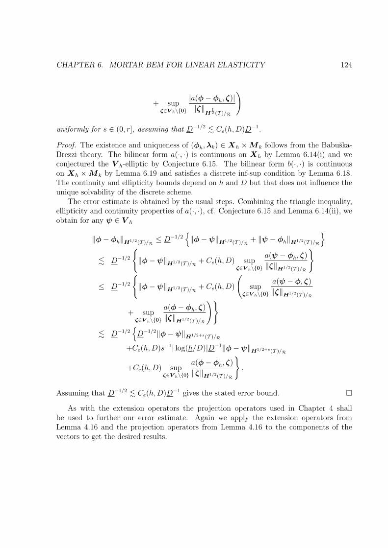
CHAPTER 6. MORTAR BEM FOR LINEAR ELASTICITY 124
+ supζ∈V h\0
|a(φ− φh, ζ)|
‖ζ‖H
12 (T )/R
)
uniformly for s ∈ (0, r], assuming that D−1/2 . Ce(h,D)D−1.
Proof. The existence and uniqueness of (φh,λk) ∈ Xh ×M k follows from the Babuska-Brezzi theory. The bilinear form a(·, ·) is continuous on Xh by Lemma 6.14(i) and weconjectured the V h-elliptic by Conjecture 6.15. The bilinear form b(·, ·) is continuouson Xh ×M k by Lemma 6.19 and satisfies a discrete inf-sup condition by Lemma 6.18.The continuity and ellipticity bounds depend on h and D but that does not influence theunique solvability of the discrete scheme.
The error estimate is obtained by the usual steps. Combining the triangle inequality,ellipticity and continuity properties of a(·, ·), cf. Conjecture 6.15 and Lemma 6.14(ii), weobtain for any ψ ∈ V h
‖φ− φh‖H1/2(T )/R≤ D−1/2
‖φ−ψ‖H1/2(T )/R
+ ‖ψ − φh‖H1/2(T )/R
. D−1/2
‖φ−ψ‖H1/2(T )/R
+ Ce(h,D) supζ∈V h\0
a(ψ − φh, ζ)
‖ζ‖H1/2(T )/R
≤ D−1/2
‖φ−ψ‖H1/2(T )/R
+ Ce(h,D)
(sup
ζ∈V h\0
a(ψ − φ, ζ)
‖ζ‖H1/2(T )/R
+ supζ∈V h\0
a(φ− φh, ζ)
‖ζ‖H1/2(T )/R
)
. D−1/2D−1/2‖φ−ψ‖H1/2+s(T )/R
+Ce(h,D)s−1| log(h/D)|D−1‖φ−ψ‖H1/2+s(T )/R
+Ce(h,D) supζ∈V h\0
a(φ− φh, ζ)
‖ζ‖H1/2(T )/R
.
Assuming that D−1/2 . Ce(h,D)D−1 gives the stated error bound.
As with the extension operators the projection operators used in Chapter 4 shallbe used to further our error estimate. Again we apply the extension operators fromLemma 4.16 and the projection operators from Lemma 4.16 to the components of thevectors to get the desired results.
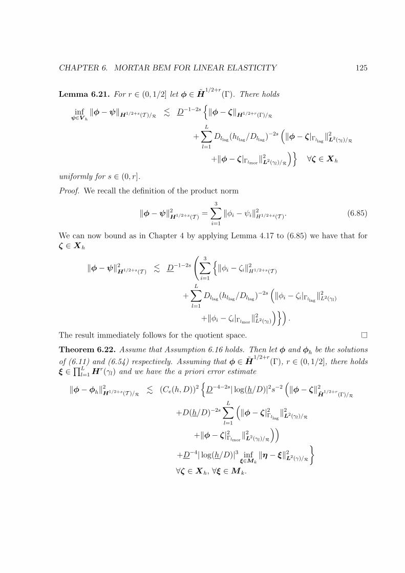
CHAPTER 6. MORTAR BEM FOR LINEAR ELASTICITY 125
Lemma 6.21. For r ∈ (0, 1/2] let φ ∈ H1/2+r
(Γ). There holds
infψ∈V h
‖φ−ψ‖H1/2+s(T )/R. D−1−2s
‖φ− ζ‖H1/2+r(Γ)/R
+L∑
l=1
Dllag(hllag/Dllag)−2s(‖φ− ζ|Γllag
‖2L2(γl)/R
+‖φ− ζ|Γlmor‖2L2(γl)/R
)∀ζ ∈Xh
uniformly for s ∈ (0, r].
Proof. We recall the definition of the product norm
‖φ−ψ‖2H1/2+s(T )
=3∑
i=1
‖φi − ψi‖2H1/2+s(T ). (6.85)
We can now bound as in Chapter 4 by applying Lemma 4.17 to (6.85) we have that forζ ∈Xh
‖φ−ψ‖2H1/2+s(T )
. D−1−2s
(3∑
i=1
‖φi − ζi‖
2H1/2+s(T )
+L∑
l=1
Dllag(hllag/Dllag)−2s(‖φi − ζi|Γllag
‖2L2(γl)
+‖φi − ζi|Γlmor‖2L2(γl)
)).
The result immediately follows for the quotient space.
Theorem 6.22. Assume that Assumption 6.16 holds. Then let φ and φh be the solutions
of (6.11) and (6.54) respectively. Assuming that φ ∈ H1/2+r
(Γ), r ∈ (0, 1/2], there holdsξ ∈
∏Ll=1H
r(γl) and we have the a priori error estimate
‖φ− φh‖2H1/2+s(T )/R
. (Ce(h,D))2D−4−2s| log(h/D)|2s−2
(‖φ− ζ‖2
H1/2+r
(Γ)/R
+D(h/D)−2s
L∑
l=1
(‖φ− ζ|2Γllag
‖2L2(γl)/R
+‖φ− ζ|2Γlmor‖2L2(γl)/R
))
+D−4| log(h/D)|3 infξ∈Mk
‖η − ξ‖2L2(γ)/R
∀ζ ∈Xh, ∀ξ ∈M k.
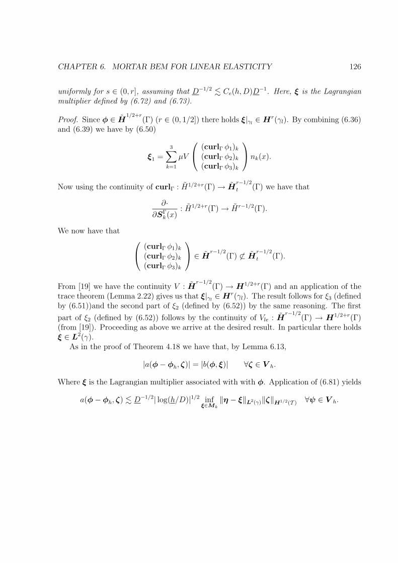
CHAPTER 6. MORTAR BEM FOR LINEAR ELASTICITY 126
uniformly for s ∈ (0, r], assuming that D−1/2 . Ce(h,D)D−1. Here, ξ is the Lagrangianmultiplier defined by (6.72) and (6.73).
Proof. Since φ ∈ H1/2+r
(Γ) (r ∈ (0, 1/2]) there holds ξ|γl∈Hr(γl). By combining (6.36)
and (6.39) we have by (6.50)
ξ1 =3∑
k=1
µV
(curlΓ φ1)k(curlΓ φ2)k(curlΓ φ3)k
nk(x).
Now using the continuity of curlΓ : H1/2+r(Γ) → Hr−1/2
t (Γ) we have that
∂·
∂SΓk (x)
: H1/2+r(Γ) → Hr−1/2(Γ).
We now have that
(curlΓ φ1)k(curlΓ φ2)k(curlΓ φ3)k
∈ H
r−1/2(Γ) 6⊂ H
r−1/2
t (Γ).
From [19] we have the continuity V : Hr−1/2
(Γ) → H1/2+r(Γ) and an application of thetrace theorem (Lemma 2.22) gives us that ξ|γl
∈Hr(γl). The result follows for ξ3 (definedby (6.51))and the second part of ξ2 (defined by (6.52)) by the same reasoning. The first
part of ξ2 (defined by (6.52)) follows by the continuity of Vle : Hr−1/2
(Γ) → H1/2+r(Γ)(from [19]). Proceeding as above we arrive at the desired result. In particular there holdsξ ∈ L2(γ).
As in the proof of Theorem 4.18 we have that, by Lemma 6.13,
|a(φ− φh, ζ)| = |b(φ, ξ)| ∀ζ ∈ V h.
Where ξ is the Lagrangian multiplier associated with with φ. Application of (6.81) yields
a(φ− φh, ζ) . D−1/2| log(h/D)|1/2 infξ∈Mk
‖η − ξ‖L2(γ)‖ζ‖H1/2(T ) ∀ψ ∈ V h.
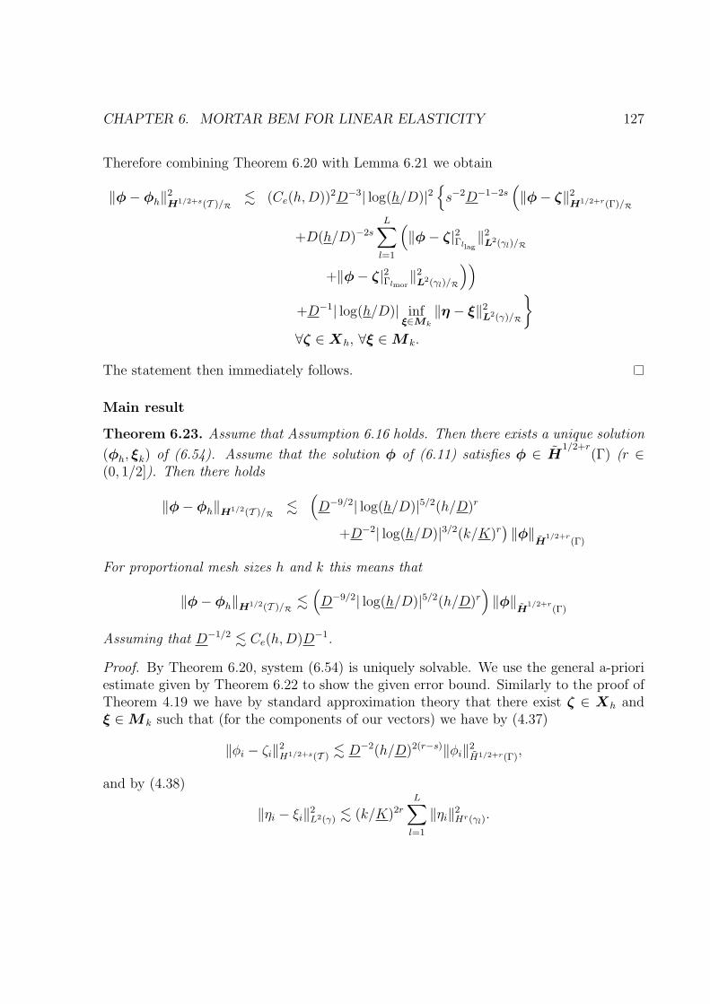
CHAPTER 6. MORTAR BEM FOR LINEAR ELASTICITY 127
Therefore combining Theorem 6.20 with Lemma 6.21 we obtain
‖φ− φh‖2H1/2+s(T )/R
. (Ce(h,D))2D−3| log(h/D)|2s−2D−1−2s
(‖φ− ζ‖2
H1/2+r(Γ)/R
+D(h/D)−2s
L∑
l=1
(‖φ− ζ|2Γllag
‖2L2(γl)/R
+‖φ− ζ|2Γlmor‖2L2(γl)/R
))
+D−1| log(h/D)| infξ∈Mk
‖η − ξ‖2L2(γ)/R
∀ζ ∈Xh, ∀ξ ∈M k.
The statement then immediately follows.
Main result
Theorem 6.23. Assume that Assumption 6.16 holds. Then there exists a unique solution
(φh, ξk) of (6.54). Assume that the solution φ of (6.11) satisfies φ ∈ H1/2+r
(Γ) (r ∈(0, 1/2]). Then there holds
‖φ− φh‖H1/2(T )/R.
(D−9/2| log(h/D)|5/2(h/D)r
+D−2| log(h/D)|3/2(k/K)r)‖φ‖
H1/2+r
(Γ)
For proportional mesh sizes h and k this means that
‖φ− φh‖H1/2(T )/R.(D−9/2| log(h/D)|5/2(h/D)r
)‖φ‖
H1/2+r
(Γ)
Assuming that D−1/2 . Ce(h,D)D−1.
Proof. By Theorem 6.20, system (6.54) is uniquely solvable. We use the general a-prioriestimate given by Theorem 6.22 to show the given error bound. Similarly to the proof ofTheorem 4.19 we have by standard approximation theory that there exist ζ ∈ Xh andξ ∈M k such that (for the components of our vectors) we have by (4.37)
‖φi − ζi‖2H1/2+s(T ) . D−2(h/D)2(r−s)‖φi‖
2H1/2+r(Γ)
,
and by (4.38)
‖ηi − ξi‖2L2(γ) . (k/K)2r
L∑
l=1
‖ηi‖2Hr(γl)
.
CHAPTER 6. MORTAR BEM FOR LINEAR ELASTICITY 128
As in the proof of Theorem 6.22 one concludes that∑L
l=1 ‖ηi‖2Hr(γl)
. ‖φi‖2H1/2+r(Γ)
. By
Lemma 2.22 one bounds, as in Theorem 4.19 (recalling that Kl is proportional to Dllag),by (4.39)
‖φi − ζi|Γllag‖L2(γl) . D
−1/2llag
s−1/2(hllag/Dllag)r−s‖φi‖H1/2+r(Γllag
),
and accordingly the mortar part ‖φ − ζlmor‖L2(γl)
. Using these bounds in Theorem 6.22and selecting s = | log(h/D)|−1 one obtains the assertion.
Chapter 7
Conclusions and Further Research
In this chapter we shall review the main results presented in the thesis and make sugges-tions for further research.
7.1 Conclusions
In Chapter 3 we presented the formulation of the BEM with Lagrangian multiplier for theLaplacian. This method allowed us to approximate the boundary conditions used in thestandard boundary element formulation. While, in itself, the method is not really a viablesolution it is the first step in allowing us to formulate a mortar style approximation to theproblem. We proved the almost quasi-optimal convergence of the scheme, and comparedit to the standard (conforming) BEM (to which it is slightly inferior).
In Chapter 4 we presented the formulation of the mortar BEM. The method allowssub-domain decompositions to be (globally) geometrically non-conforming and meshes tobe quasi-uniform only on sub-domains. However we do have the restriction of Assump-tion 4.2. We were able to prove almost quasi-optimal convergence of the scheme, and itsdependence upon sub-domain size. However these results may not be optimal and maybe able to be improved upon. The result is not optimal because of the dependence onsub-domain size of some of the estimates. Also when bounding sub-domain size we havenot always used optimal bounds, for example we replaced D−2ǫ
i by D−1i in (4.18) and
D−1−2s by D−2 in (4.37). The slight loss of optimality is caused by the lack of a traceoperator for functions in H1/2.
In Chapter 5 we presented numerical results for both the boundary element methodwith Lagrangian multiplier and for the mortar boundary element method. These resultsunderlined the theoretical results of the previous chapters. In particular for the mortarboundary element method we were able to show the effects of defining the Lagrangianmultipliers in different ways on the accuracy of the approximation. We were also able to
129
CHAPTER 7. CONCLUSIONS AND FURTHER RESEARCH 130
show results for a decomposition of sub-domains which did not satisfy Assumption 4.2.In Chapter 6 we presented the formulation of the mortar boundary element method for
linear elasticity. These results are an extension of the work in Chapter 4. We were unableto prove the Vh ellipticity of the bilinear form a(·, ·). Instead we presented Conjecture 6.15and discussed some of the problems we encountered in Remark 6.17. Assuming that theconjecture was true we were able to prove a quasi-optimal result similar to that provedin Chapter 4.
7.2 Suggestions for further research
We shall now present suggestions relating to how the work in this thesis can be extended.We also include some unanswered questions which arose during the preparation of thisthesis.
In Chapter 3 we presented the formulation of the BEM with Lagrangian multiplierfor the Laplacian. We presented an error estimate which showed how the accuracy ofthe solution depended on the mesh size. The obvious extension to this is to extend thish-version (dependence on sub-domain size) to a p-version (dependence on polynomialdegree), and eventually a full hp-version (dependence on both mesh size and polynomialdegree). By a p-version we mean a scheme where instead of reducing the mesh size toimprove the accuracy of the approximation we increase the polynomial degree on eachelement to improve the accuracy. A full hp-scheme would be one where we would be ableto both decrease the mesh size and increase the polynomial degree to get an improvedapproximation. Not only would we be able to gain a better approximation through the useof higher degree polynomials defined over the domain (we used piecewise linear functionsin Chapter 3) we must use higher degree polynomials for the Lagrangian multiplier space(we used piecewise constant functions over a coarsened mesh in Chapter 3). This wouldmake the analysis and implementation of the method more complicated.
In Chapter 4 we presented the formulation of the mortar boundary element method.As in Chapter 3 we presented an error estimate which showed how the accuracy of theapproximation depended upon mesh size (and also upon sub-domain size). Again theobvious extension is to develop a p-version and then a full hp-scheme. The ability touse different mesh sizes and different polynomial degrees on separate sub-domains wouldbe a useful tool. Also, the ability to be able to use polynomials of different degreeson each interface in the definition of the Lagrangian multiplier space would lead to abetter approximation. Another extension would be to relax Assumption 4.2, which statedthat each interface was a whole edge of at least one of the sub-domains that form theinterface. This is a restriction that would be useful to remove, and the numerical results(see Section 5.3.3) appear to suggest that the assumption can be relaxed.
CHAPTER 7. CONCLUSIONS AND FURTHER RESEARCH 131
In Chapter 6 we presented the formulation of the mortar BEM for linear elasticity.The first thing to be further examined is Conjecture 6.15 which states the ellipticity ofthe bilinear form a(·, ·) on the constrained space. As discussed in Remark 6.17 the proofof this conjecture has obstacles to be overcome. As in the previous paragraph the resultscould be extended to a full hp-scheme for a more versatile and accurate method. Therelaxation of Assumption 4.2 would also have a knock on effect into the results of thischapter.
Further objectives beyond what have been stated above are many and varied. Otheroperators could be examined, such as the Helmholtz or Maxwell operators which wouldhave new difficulties as they do not possess the same properties as those examined in thisthesis (the Helmholtz operator is indefinite, and the Maxwell operator is not elliptic orpositive definite). Related problems from numerical linear algebra could also be examined.These may include the analysis of specific solvers and preconditioners for the systemsdescribed in this thesis. Related to this point is the the notion of parallel implementationsof the mortar BEM to make use of the independence of the sub-domains. By this wemean that different processors could handle different parts (sub-domains) of the problem,improving the speed and efficiency of the scheme.
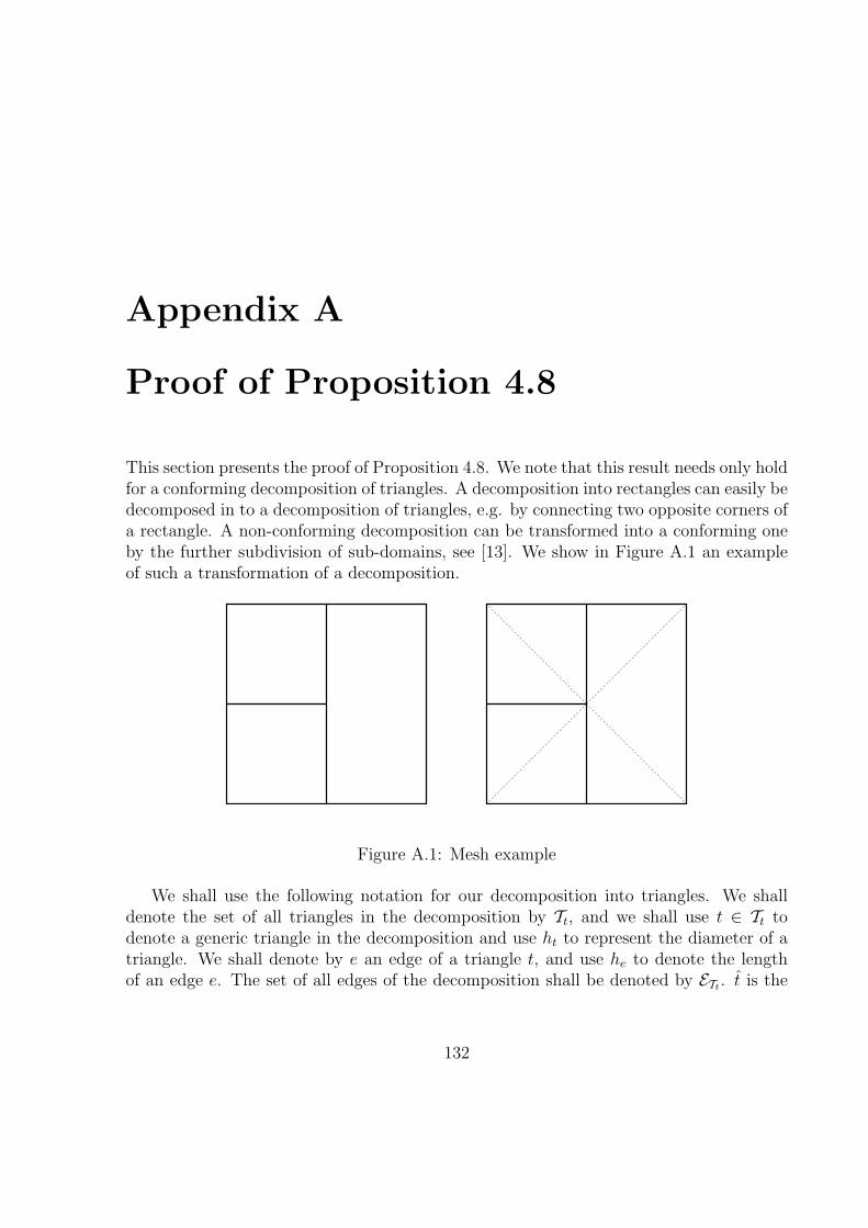
Appendix A
Proof of Proposition 4.8
This section presents the proof of Proposition 4.8. We note that this result needs only holdfor a conforming decomposition of triangles. A decomposition into rectangles can easily bedecomposed in to a decomposition of triangles, e.g. by connecting two opposite corners ofa rectangle. A non-conforming decomposition can be transformed into a conforming oneby the further subdivision of sub-domains, see [13]. We show in Figure A.1 an exampleof such a transformation of a decomposition.
Figure A.1: Mesh example
We shall use the following notation for our decomposition into triangles. We shalldenote the set of all triangles in the decomposition by Tt, and we shall use t ∈ Tt todenote a generic triangle in the decomposition and use ht to represent the diameter of atriangle. We shall denote by e an edge of a triangle t, and use he to denote the lengthof an edge e. The set of all edges of the decomposition shall be denoted by ETt . t is the
132
APPENDIX A. PROOF OF PROPOSITION 4.8 133
reference triangle as described earlier. We shall also use the space
VTt := v ∈ L2(Γ) : (Iv)|t ∈ P1(t) for any t ∈ Tt and v is continuous
at the common side of any two neighbouring
sub-domains and v|∂Γ = 0.
Following [13] we define the following interpolation operators,
I :∏
t∈Tt
H1(t) → VTt
(Iv)(me) :=1
he
∫
e
v,
where me is the midpoint of the edge e, and v is the average of the values of v ap-proaching e from the elements sharing e, and
Π :∏
t∈Tt
H1(t) →∏
t∈Tt
P1(t)
(Πv)(me) :=1
he
∫
e
v|t.
Note that there holds, for [v] the jump of v over the edge e,
(Iv − Πv)|t(me) =1
2he
∫
e
[v].
Lemma A.1. For all ǫ ∈ (0.1/2), v ∈ H1/2+ǫ(Tt), and t ∈ Tt,
∑
t∈Tt
|Iv − Πv|2H1/2+ǫ(t) .∑
e∈E(t)\∂Γ
h−1−2ǫe |
∫
e
[v]|2 (A.1)
∑
t∈Tt
|Πv|2H1/2+ǫ(t) .∑
t∈Tt
ǫ−1|v|2H1/2+ǫ(t) (A.2)
∑
t∈Tt
‖v − Πv‖2L2(Γ) .
∑
t∈Tt
ǫ−1h1+2ǫt |v|2H1/2+ǫ(t). (A.3)
Proof. For (A.1) we have from [13] that
∑
t∈Tt
|Iv − Πv|2H1(t) .∑
e∈E(t)\∂Γ
h−2e |
∫
e
[v]|2,
∑
t∈Tt
‖Iv − Πv‖2L2(t)
.∑
e∈E(t)\∂Γ
|
∫
e
[v]|2.
The result follows by interpolation. For (A.2) and (A.3) we simply follow the proof of [30,Lemma 9].
APPENDIX A. PROOF OF PROPOSITION 4.8 134
Lemma A.2. For all ǫ ∈ (0, 1/2) and v ∈ H1/2+ǫ(Tt)
∑
t∈Tt
|Iv|2H1/2+ǫ(Tt).
∑
t∈Tt
ǫ−1|v|2H1/2+ǫ(t) +∑
e∈E(t)\∂Γ
h−1−2ǫe |
∫
e
[v]|2 (A.4)
‖v − Iv‖2L2(Γ) .
∑
t∈Tt
ǫ−1h1+2ǫt |v|2H1/2+ǫ(t) +
∑
e∈E(t)\∂Γ
|
∫
e
[v]|2. (A.5)
Proof. We simply follow the proof of [30, Lemma 10].
Let WTt be the space of continuous P2 finite elements on Tt. Let ETt : VTt → WTt bethe interpolation operator that takes values at midpoints of sides and average values atvertices. Let FTt : WTt → VTt be the interpolation operator that takes values only on themidpoints of the sides. Note that FTtETt = I in VTt , and that in particular Iv ∈ VTt forv ∈ H1/2+ǫ(Tt).
Lemma A.3. For all r ∈ (0, 1), and ∀ξ ∈ VTt
‖ETtξ − ξ‖2L2(Γ) .
∑
t∈Tt
h2rt |ξ|
2Hr(t) (A.6)
‖ETtξ‖L2(Γ) ≈ ‖ξ‖L2(Γ) (A.7)
|ETtξ|2L2(Γ) .
∑
t∈Tt
|ξ|2Hr(t). (A.8)
Proof. We simply follow the proof of [30, Lemma 11].
Lemma A.4. For all r ∈ (0, 1) and for all ξ ∈ VTt
‖ξ‖2L2(Γ) .
∑
t∈Tt
|ξ|2Hr(t). (A.9)
Proof. Again we follow the proof of [30, Proposition 12]. We note that the term |∫Γξ| is
not included as a result of our boundary conditions, the constant function 0 is the onlyadmissible constant function due the boundary conditions and the continuity conditionacross a midpoint of a side imposed on functions in VTt .
Proposition A.5. For v ∈∏n
i=1H1/2+ǫ(Tt)
‖v‖2L2(Γ) .
∑
t∈Tt
ǫ−1|v|2H1/2+ǫ(t) +∑
e∈E(t)\∂Γ
h−1−2ǫe |
∫
e
[v]|2. (A.10)
APPENDIX A. PROOF OF PROPOSITION 4.8 135
Proof. For v ∈∏
t∈TtH1/2+ǫ(Tt) by the triangle inequality and Lemma A.4
‖v‖2L2(Γ) = ‖v + Iv − Iv‖2
L2(Γ)
. ‖v − Iv‖2L2(Γ) + ‖Iv‖2
L2(Γ)
. ‖v − Iv‖2L2(Γ) +
∑
t∈Tt
|Iv|2H1/2+ǫ(t).
We can now apply (A.4) and (A.5) to get the stated result.
Proof of Proposition 4.8. It is immediate that the jump across any artificial edgeswhich have been added to the original decomposition into sub-domains (Γi, i ∈ 1, . . . , Nsee Section 4.1.2) to turn the decomposition into a conforming decomposition of trianglesis equal to zero, as in the original decomposition the function is continuous across thisedge at all points. We are thus left only with jumps across the original edges. We alsonote that
n∏
i=1
H1/2+ǫ(Γi) ⊂∏
t∈Tt
H1/2+ǫ(t).
The result then follows.
Appendix B
Tables Of Numerical Results
In this appendix we present in tabular form the numerical results presented in the figuresin Chapter 5. We present the numerical results at the precision of three significant figuresfor conciseness.
136
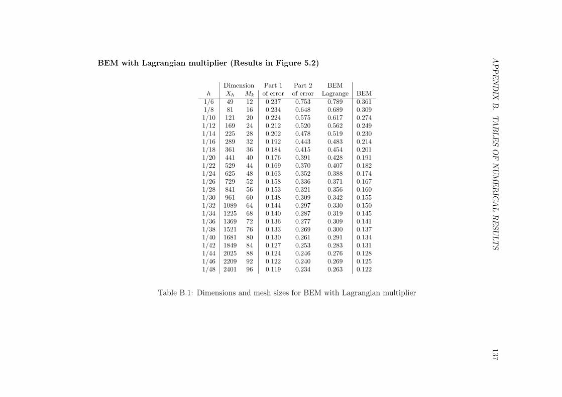
AP
PE
ND
IXB
.TA
BLE
SO
FN
UM
ER
ICA
LR
ESU
LT
S137
BEM with Lagrangian multiplier (Results in Figure 5.2)
Dimension Part 1 Part 2 BEMh Xh Mk of error of error Lagrange BEM
1/6 49 12 0.237 0.753 0.789 0.3611/8 81 16 0.234 0.648 0.689 0.3091/10 121 20 0.224 0.575 0.617 0.2741/12 169 24 0.212 0.520 0.562 0.2491/14 225 28 0.202 0.478 0.519 0.2301/16 289 32 0.192 0.443 0.483 0.2141/18 361 36 0.184 0.415 0.454 0.2011/20 441 40 0.176 0.391 0.428 0.1911/22 529 44 0.169 0.370 0.407 0.1821/24 625 48 0.163 0.352 0.388 0.1741/26 729 52 0.158 0.336 0.371 0.1671/28 841 56 0.153 0.321 0.356 0.1601/30 961 60 0.148 0.309 0.342 0.1551/32 1089 64 0.144 0.297 0.330 0.1501/34 1225 68 0.140 0.287 0.319 0.1451/36 1369 72 0.136 0.277 0.309 0.1411/38 1521 76 0.133 0.269 0.300 0.1371/40 1681 80 0.130 0.261 0.291 0.1341/42 1849 84 0.127 0.253 0.283 0.1311/44 2025 88 0.124 0.246 0.276 0.1281/46 2209 92 0.122 0.240 0.269 0.1251/48 2401 96 0.119 0.234 0.263 0.122
Table B.1: Dimensions and mesh sizes for BEM with Lagrangian multiplier
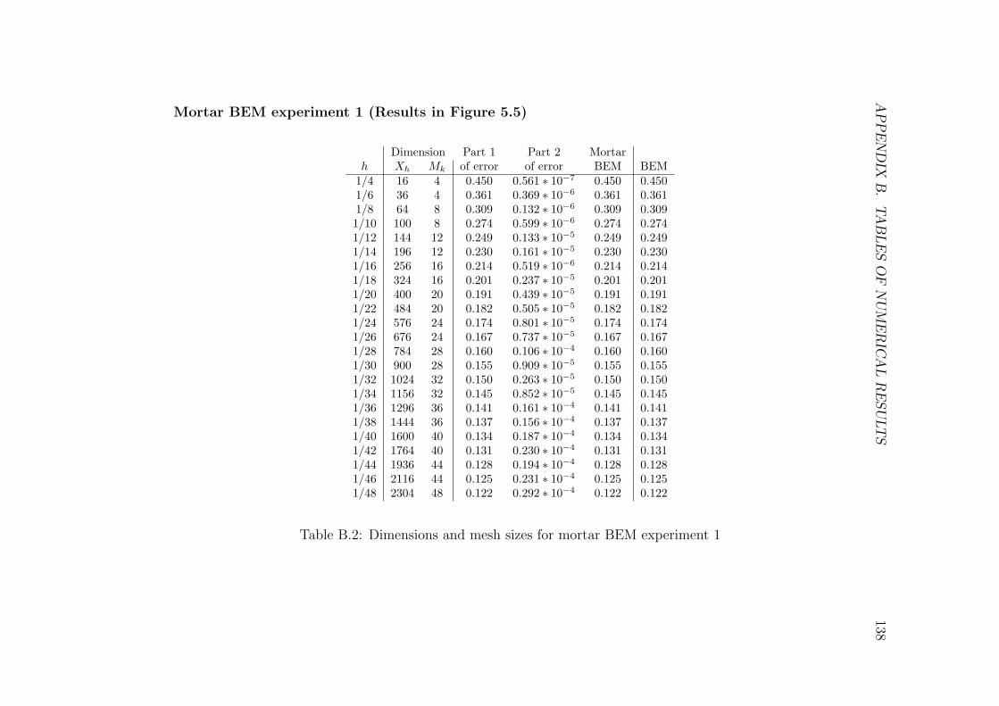
AP
PE
ND
IXB
.TA
BLE
SO
FN
UM
ER
ICA
LR
ESU
LT
S138
Mortar BEM experiment 1 (Results in Figure 5.5)
Dimension Part 1 Part 2 Mortarh Xh Mk of error of error BEM BEM
1/4 16 4 0.450 0.561 ∗ 10−7 0.450 0.4501/6 36 4 0.361 0.369 ∗ 10−6 0.361 0.3611/8 64 8 0.309 0.132 ∗ 10−6 0.309 0.3091/10 100 8 0.274 0.599 ∗ 10−6 0.274 0.2741/12 144 12 0.249 0.133 ∗ 10−5 0.249 0.2491/14 196 12 0.230 0.161 ∗ 10−5 0.230 0.2301/16 256 16 0.214 0.519 ∗ 10−6 0.214 0.2141/18 324 16 0.201 0.237 ∗ 10−5 0.201 0.2011/20 400 20 0.191 0.439 ∗ 10−5 0.191 0.1911/22 484 20 0.182 0.505 ∗ 10−5 0.182 0.1821/24 576 24 0.174 0.801 ∗ 10−5 0.174 0.1741/26 676 24 0.167 0.737 ∗ 10−5 0.167 0.1671/28 784 28 0.160 0.106 ∗ 10−4 0.160 0.1601/30 900 28 0.155 0.909 ∗ 10−5 0.155 0.1551/32 1024 32 0.150 0.263 ∗ 10−5 0.150 0.1501/34 1156 32 0.145 0.852 ∗ 10−5 0.145 0.1451/36 1296 36 0.141 0.161 ∗ 10−4 0.141 0.1411/38 1444 36 0.137 0.156 ∗ 10−4 0.137 0.1371/40 1600 40 0.134 0.187 ∗ 10−4 0.134 0.1341/42 1764 40 0.131 0.230 ∗ 10−4 0.131 0.1311/44 1936 44 0.128 0.194 ∗ 10−4 0.128 0.1281/46 2116 44 0.125 0.231 ∗ 10−4 0.125 0.1251/48 2304 48 0.122 0.292 ∗ 10−4 0.122 0.122
Table B.2: Dimensions and mesh sizes for mortar BEM experiment 1
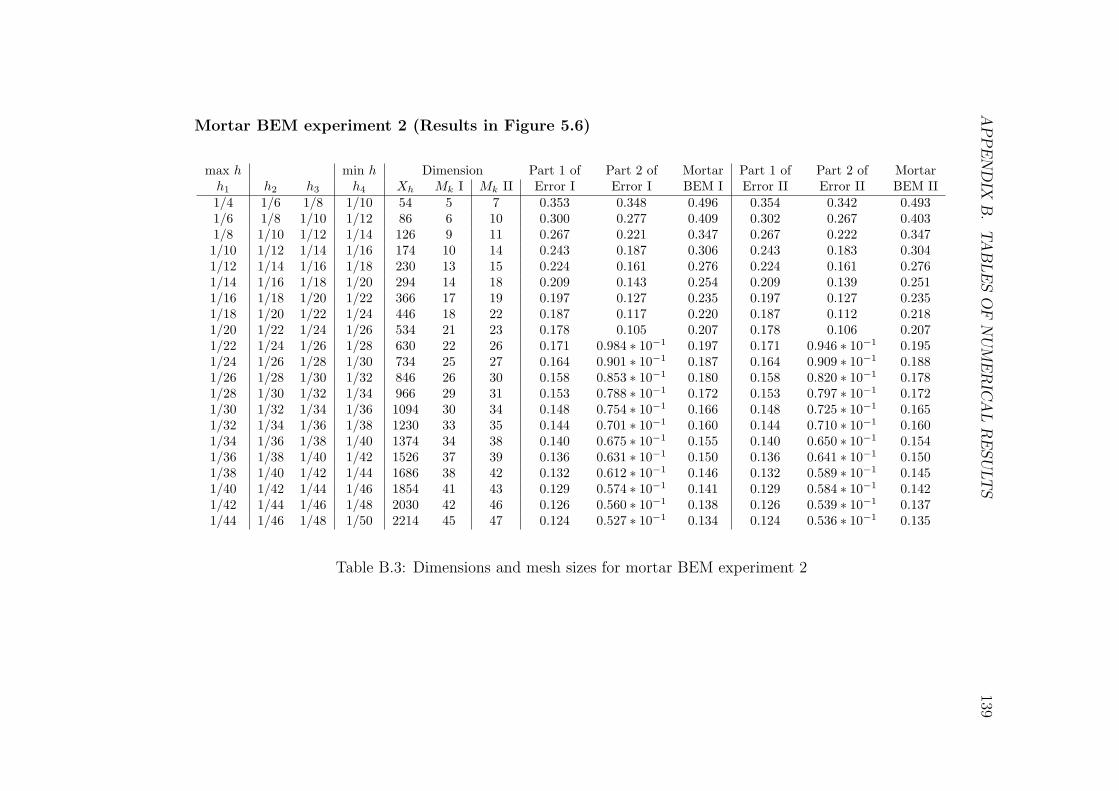
AP
PE
ND
IXB
.TA
BLE
SO
FN
UM
ER
ICA
LR
ESU
LT
S139
Mortar BEM experiment 2 (Results in Figure 5.6)
max h min h Dimension Part 1 of Part 2 of Mortar Part 1 of Part 2 of Mortarh1 h2 h3 h4 Xh Mk I Mk II Error I Error I BEM I Error II Error II BEM II1/4 1/6 1/8 1/10 54 5 7 0.353 0.348 0.496 0.354 0.342 0.4931/6 1/8 1/10 1/12 86 6 10 0.300 0.277 0.409 0.302 0.267 0.4031/8 1/10 1/12 1/14 126 9 11 0.267 0.221 0.347 0.267 0.222 0.3471/10 1/12 1/14 1/16 174 10 14 0.243 0.187 0.306 0.243 0.183 0.3041/12 1/14 1/16 1/18 230 13 15 0.224 0.161 0.276 0.224 0.161 0.2761/14 1/16 1/18 1/20 294 14 18 0.209 0.143 0.254 0.209 0.139 0.2511/16 1/18 1/20 1/22 366 17 19 0.197 0.127 0.235 0.197 0.127 0.2351/18 1/20 1/22 1/24 446 18 22 0.187 0.117 0.220 0.187 0.112 0.2181/20 1/22 1/24 1/26 534 21 23 0.178 0.105 0.207 0.178 0.106 0.2071/22 1/24 1/26 1/28 630 22 26 0.171 0.984 ∗ 10−1 0.197 0.171 0.946 ∗ 10−1 0.1951/24 1/26 1/28 1/30 734 25 27 0.164 0.901 ∗ 10−1 0.187 0.164 0.909 ∗ 10−1 0.1881/26 1/28 1/30 1/32 846 26 30 0.158 0.853 ∗ 10−1 0.180 0.158 0.820 ∗ 10−1 0.1781/28 1/30 1/32 1/34 966 29 31 0.153 0.788 ∗ 10−1 0.172 0.153 0.797 ∗ 10−1 0.1721/30 1/32 1/34 1/36 1094 30 34 0.148 0.754 ∗ 10−1 0.166 0.148 0.725 ∗ 10−1 0.1651/32 1/34 1/36 1/38 1230 33 35 0.144 0.701 ∗ 10−1 0.160 0.144 0.710 ∗ 10−1 0.1601/34 1/36 1/38 1/40 1374 34 38 0.140 0.675 ∗ 10−1 0.155 0.140 0.650 ∗ 10−1 0.1541/36 1/38 1/40 1/42 1526 37 39 0.136 0.631 ∗ 10−1 0.150 0.136 0.641 ∗ 10−1 0.1501/38 1/40 1/42 1/44 1686 38 42 0.132 0.612 ∗ 10−1 0.146 0.132 0.589 ∗ 10−1 0.1451/40 1/42 1/44 1/46 1854 41 43 0.129 0.574 ∗ 10−1 0.141 0.129 0.584 ∗ 10−1 0.1421/42 1/44 1/46 1/48 2030 42 46 0.126 0.560 ∗ 10−1 0.138 0.126 0.539 ∗ 10−1 0.1371/44 1/46 1/48 1/50 2214 45 47 0.124 0.527 ∗ 10−1 0.134 0.124 0.536 ∗ 10−1 0.135
Table B.3: Dimensions and mesh sizes for mortar BEM experiment 2
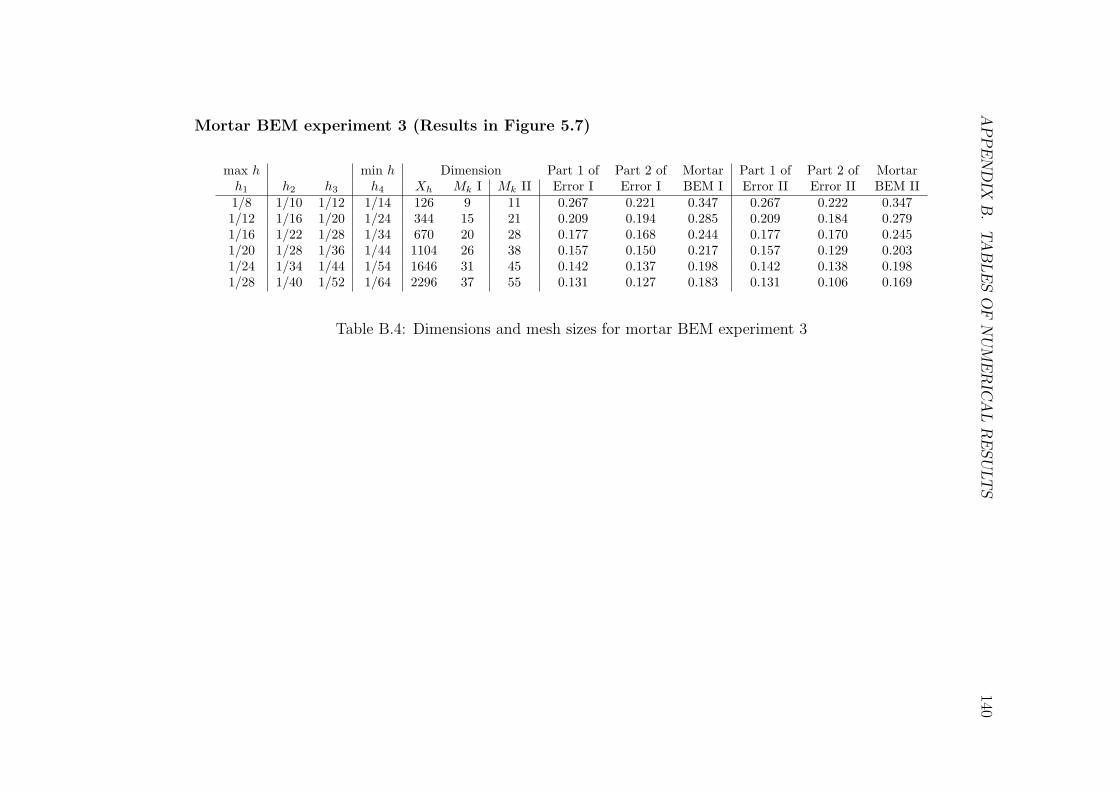
AP
PE
ND
IXB
.TA
BLE
SO
FN
UM
ER
ICA
LR
ESU
LT
S140
Mortar BEM experiment 3 (Results in Figure 5.7)
max h min h Dimension Part 1 of Part 2 of Mortar Part 1 of Part 2 of Mortarh1 h2 h3 h4 Xh Mk I Mk II Error I Error I BEM I Error II Error II BEM II1/8 1/10 1/12 1/14 126 9 11 0.267 0.221 0.347 0.267 0.222 0.3471/12 1/16 1/20 1/24 344 15 21 0.209 0.194 0.285 0.209 0.184 0.2791/16 1/22 1/28 1/34 670 20 28 0.177 0.168 0.244 0.177 0.170 0.2451/20 1/28 1/36 1/44 1104 26 38 0.157 0.150 0.217 0.157 0.129 0.2031/24 1/34 1/44 1/54 1646 31 45 0.142 0.137 0.198 0.142 0.138 0.1981/28 1/40 1/52 1/64 2296 37 55 0.131 0.127 0.183 0.131 0.106 0.169
Table B.4: Dimensions and mesh sizes for mortar BEM experiment 3
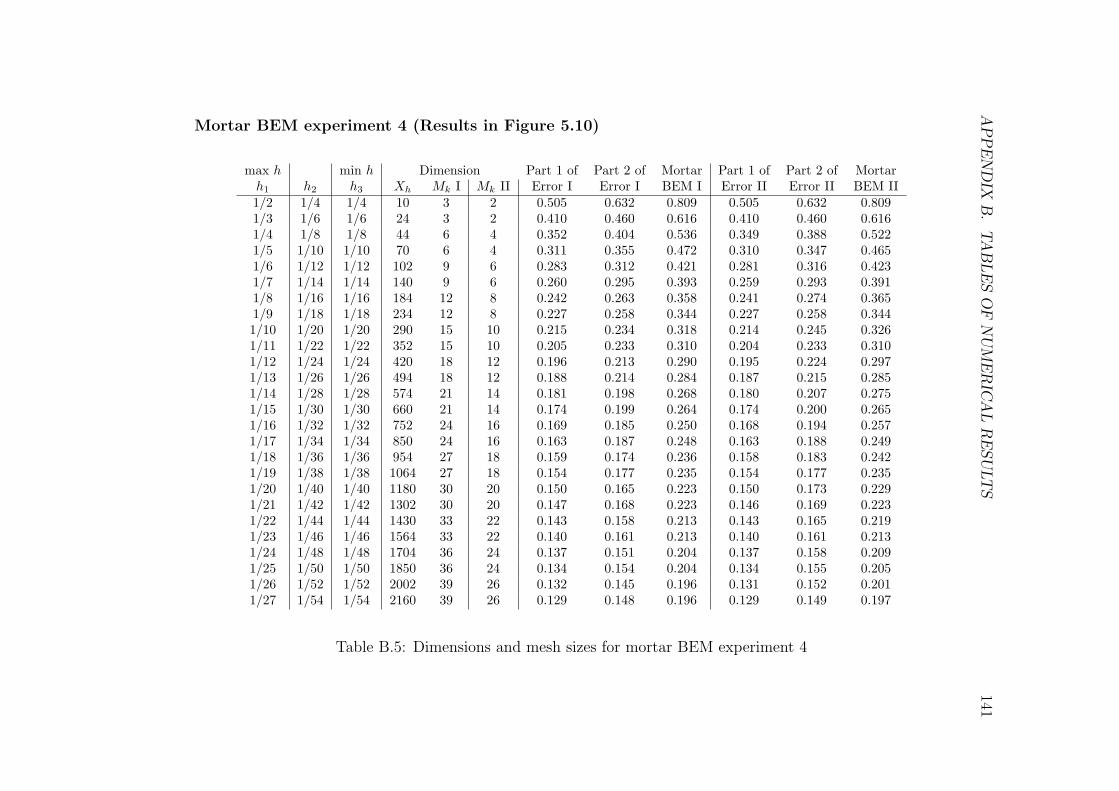
AP
PE
ND
IXB
.TA
BLE
SO
FN
UM
ER
ICA
LR
ESU
LT
S141
Mortar BEM experiment 4 (Results in Figure 5.10)
max h min h Dimension Part 1 of Part 2 of Mortar Part 1 of Part 2 of Mortarh1 h2 h3 Xh Mk I Mk II Error I Error I BEM I Error II Error II BEM II1/2 1/4 1/4 10 3 2 0.505 0.632 0.809 0.505 0.632 0.8091/3 1/6 1/6 24 3 2 0.410 0.460 0.616 0.410 0.460 0.6161/4 1/8 1/8 44 6 4 0.352 0.404 0.536 0.349 0.388 0.5221/5 1/10 1/10 70 6 4 0.311 0.355 0.472 0.310 0.347 0.4651/6 1/12 1/12 102 9 6 0.283 0.312 0.421 0.281 0.316 0.4231/7 1/14 1/14 140 9 6 0.260 0.295 0.393 0.259 0.293 0.3911/8 1/16 1/16 184 12 8 0.242 0.263 0.358 0.241 0.274 0.3651/9 1/18 1/18 234 12 8 0.227 0.258 0.344 0.227 0.258 0.3441/10 1/20 1/20 290 15 10 0.215 0.234 0.318 0.214 0.245 0.3261/11 1/22 1/22 352 15 10 0.205 0.233 0.310 0.204 0.233 0.3101/12 1/24 1/24 420 18 12 0.196 0.213 0.290 0.195 0.224 0.2971/13 1/26 1/26 494 18 12 0.188 0.214 0.284 0.187 0.215 0.2851/14 1/28 1/28 574 21 14 0.181 0.198 0.268 0.180 0.207 0.2751/15 1/30 1/30 660 21 14 0.174 0.199 0.264 0.174 0.200 0.2651/16 1/32 1/32 752 24 16 0.169 0.185 0.250 0.168 0.194 0.2571/17 1/34 1/34 850 24 16 0.163 0.187 0.248 0.163 0.188 0.2491/18 1/36 1/36 954 27 18 0.159 0.174 0.236 0.158 0.183 0.2421/19 1/38 1/38 1064 27 18 0.154 0.177 0.235 0.154 0.177 0.2351/20 1/40 1/40 1180 30 20 0.150 0.165 0.223 0.150 0.173 0.2291/21 1/42 1/42 1302 30 20 0.147 0.168 0.223 0.146 0.169 0.2231/22 1/44 1/44 1430 33 22 0.143 0.158 0.213 0.143 0.165 0.2191/23 1/46 1/46 1564 33 22 0.140 0.161 0.213 0.140 0.161 0.2131/24 1/48 1/48 1704 36 24 0.137 0.151 0.204 0.137 0.158 0.2091/25 1/50 1/50 1850 36 24 0.134 0.154 0.204 0.134 0.155 0.2051/26 1/52 1/52 2002 39 26 0.132 0.145 0.196 0.131 0.152 0.2011/27 1/54 1/54 2160 39 26 0.129 0.148 0.196 0.129 0.149 0.197
Table B.5: Dimensions and mesh sizes for mortar BEM experiment 4
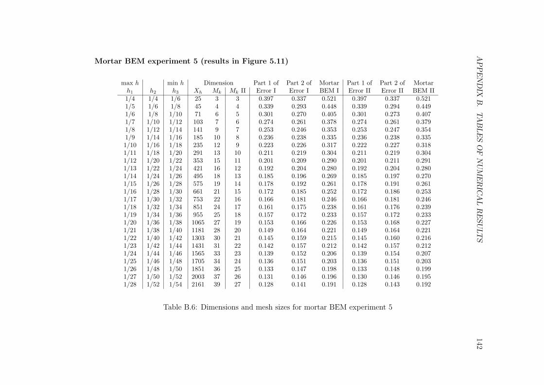
AP
PE
ND
IXB
.TA
BLE
SO
FN
UM
ER
ICA
LR
ESU
LT
S142
Mortar BEM experiment 5 (results in Figure 5.11)
max h min h Dimension Part 1 of Part 2 of Mortar Part 1 of Part 2 of Mortarh1 h2 h3 Xh Mk Mk II Error I Error I BEM I Error II Error II BEM II1/4 1/4 1/6 25 3 3 0.397 0.337 0.521 0.397 0.337 0.5211/5 1/6 1/8 45 4 4 0.339 0.293 0.448 0.339 0.294 0.4491/6 1/8 1/10 71 6 5 0.301 0.270 0.405 0.301 0.273 0.4071/7 1/10 1/12 103 7 6 0.274 0.261 0.378 0.274 0.261 0.3791/8 1/12 1/14 141 9 7 0.253 0.246 0.353 0.253 0.247 0.3541/9 1/14 1/16 185 10 8 0.236 0.238 0.335 0.236 0.238 0.3351/10 1/16 1/18 235 12 9 0.223 0.226 0.317 0.222 0.227 0.3181/11 1/18 1/20 291 13 10 0.211 0.219 0.304 0.211 0.219 0.3041/12 1/20 1/22 353 15 11 0.201 0.209 0.290 0.201 0.211 0.2911/13 1/22 1/24 421 16 12 0.192 0.204 0.280 0.192 0.204 0.2801/14 1/24 1/26 495 18 13 0.185 0.196 0.269 0.185 0.197 0.2701/15 1/26 1/28 575 19 14 0.178 0.192 0.261 0.178 0.191 0.2611/16 1/28 1/30 661 21 15 0.172 0.185 0.252 0.172 0.186 0.2531/17 1/30 1/32 753 22 16 0.166 0.181 0.246 0.166 0.181 0.2461/18 1/32 1/34 851 24 17 0.161 0.175 0.238 0.161 0.176 0.2391/19 1/34 1/36 955 25 18 0.157 0.172 0.233 0.157 0.172 0.2331/20 1/36 1/38 1065 27 19 0.153 0.166 0.226 0.153 0.168 0.2271/21 1/38 1/40 1181 28 20 0.149 0.164 0.221 0.149 0.164 0.2211/22 1/40 1/42 1303 30 21 0.145 0.159 0.215 0.145 0.160 0.2161/23 1/42 1/44 1431 31 22 0.142 0.157 0.212 0.142 0.157 0.2121/24 1/44 1/46 1565 33 23 0.139 0.152 0.206 0.139 0.154 0.2071/25 1/46 1/48 1705 34 24 0.136 0.151 0.203 0.136 0.151 0.2031/26 1/48 1/50 1851 36 25 0.133 0.147 0.198 0.133 0.148 0.1991/27 1/50 1/52 2003 37 26 0.131 0.146 0.196 0.130 0.146 0.1951/28 1/52 1/54 2161 39 27 0.128 0.141 0.191 0.128 0.143 0.192
Table B.6: Dimensions and mesh sizes for mortar BEM experiment 5
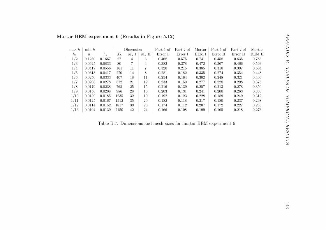
AP
PE
ND
IXB
.TA
BLE
SO
FN
UM
ER
ICA
LR
ESU
LT
S143
Mortar BEM experiment 6 (Results in Figure 5.12)
max h min h Dimension Part 1 of Part 2 of Mortar Part 1 of Part 2 of Mortarh3 h1 h2 Xh Mk I Mk II Error I Error I BEM I Error II Error II BEM II1/2 0.1250 0.1667 27 4 3 0.468 0.575 0.741 0.458 0.635 0.7831/3 0.0625 0.0833 80 7 4 0.382 0.278 0.472 0.367 0.466 0.5931/4 0.0417 0.0556 161 11 7 0.320 0.215 0.385 0.310 0.397 0.5041/5 0.0313 0.0417 270 14 8 0.281 0.182 0.335 0.274 0.354 0.4481/6 0.0250 0.0333 407 18 11 0.254 0.164 0.302 0.248 0.321 0.4061/7 0.0208 0.0278 572 21 12 0.233 0.150 0.277 0.228 0.298 0.3751/8 0.0179 0.0238 765 25 15 0.216 0.139 0.257 0.213 0.278 0.3501/9 0.0156 0.0208 986 28 16 0.203 0.131 0.241 0.200 0.263 0.3301/10 0.0139 0.0185 1235 32 19 0.192 0.123 0.228 0.189 0.249 0.3121/11 0.0125 0.0167 1512 35 20 0.182 0.118 0.217 0.180 0.237 0.2981/12 0.0114 0.0152 1817 39 23 0.174 0.112 0.207 0.172 0.227 0.2851/13 0.0104 0.0139 2150 42 24 0.166 0.108 0.199 0.165 0.218 0.273
Table B.7: Dimensions and mesh sizes for mortar BEM experiment 6

AP
PE
ND
IXB
.TA
BLE
SO
FN
UM
ER
ICA
LR
ESU
LT
S144
Mortar BEM experiment 7 (Results in Figure 5.15)
Dimension Part 1 of Part 2 of Mortar Part 1 of Part 2 of Mortarmax h min h Xh Mk I Mk II Error I Error I BEM I Error II Error II BEM II7/20 1/4 16 4 4 0.449 0.581 0.734 0.449 0.581 0.7347/30 1/6 36 4 4 0.356 0.499 0.613 0.356 0.499 0.6137/40 1/8 64 8 8 0.311 0.301 0.433 0.311 0.301 0.4337/50 1/10 100 8 8 0.275 0.327 0.427 0.271 0.319 0.4197/60 1/12 144 12 12 0.250 0.238 0.345 0.250 0.238 0.3451/10 1/14 196 12 12 0.229 0.270 0.354 0.230 0.256 0.3447/80 1/16 256 16 16 0.215 0.200 0.294 0.215 0.200 0.2947/90 1/18 324 16 16 0.201 0.233 0.308 0.202 0.215 0.2957/100 1/20 400 20 20 0.191 0.178 0.261 0.191 0.178 0.2617/110 1/22 484 20 20 0.182 0.208 0.276 0.182 0.191 0.2647/120 1/24 576 24 24 0.174 0.162 0.238 0.174 0.162 0.2387/130 1/26 676 24 24 0.167 0.189 0.252 0.167 0.173 0.2411/20 1/28 784 28 28 0.161 0.150 0.220 0.161 0.150 0.2207/150 1/30 900 28 28 0.155 0.175 0.234 0.155 0.159 0.2237/160 1/32 1024 32 32 0.150 0.140 0.205 0.150 0.140 0.2057/170 1/34 1156 32 32 0.145 0.163 0.218 0.146 0.148 0.2087/180 1/36 1296 36 36 0.142 0.132 0.194 0.142 0.132 0.1947/190 1/38 1444 36 36 0.137 0.153 0.206 0.138 0.139 0.1967/200 1/40 1600 40 40 0.134 0.125 0.183 0.134 0.125 0.1831/30 1/42 1764 40 40 0.131 0.145 0.195 0.131 0.132 0.1867/220 1/44 1936 44 44 0.128 0.119 0.175 0.128 0.119 0.1757/230 1/46 2116 44 44 0.125 0.138 0.186 0.125 0.125 0.1777/240 1/48 2304 48 48 0.122 0.114 0.167 0.122 0.114 0.167
Table B.8: Dimensions and mesh sizes for mortar BEM experiment 7
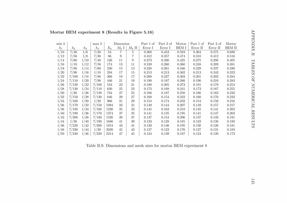
AP
PE
ND
IXB
.TA
BLE
SO
FN
UM
ER
ICA
LR
ESU
LT
S145
Mortar BEM experiment 8 (Results in Figure 5.16)
min h max h Dimension Part 1 of Part 2 of Mortar Part 1 of Part 2 of Mortarh1 h2 h3 h4 Xh Mk I Mk II Error I Error I BEM I Error II Error II BEM II
1/10 7/40 1/6 7/20 54 7 5 0.368 0.453 0.583 0.364 0.575 0.6801/12 7/50 1/8 7/30 86 9 7 0.312 0.357 0.474 0.310 0.412 0.5161/14 7/60 1/10 7/40 126 11 9 0.273 0.326 0.425 0.275 0.298 0.4051/16 1/10 1/12 7/50 174 13 11 0.249 0.260 0.360 0.248 0.289 0.3811/18 7/80 1/14 7/60 230 15 13 0.228 0.261 0.346 0.229 0.237 0.3301/20 7/90 1/16 1/10 294 17 15 0.213 0.213 0.302 0.213 0.243 0.3231/22 7/100 1/18 7/80 366 19 17 0.200 0.227 0.303 0.201 0.202 0.2841/24 7/110 1/20 7/90 446 21 19 0.190 0.187 0.266 0.190 0.210 0.2831/26 7/120 1/22 7/100 534 23 21 0.180 0.205 0.273 0.181 0.179 0.2541/28 7/130 1/24 7/110 630 25 23 0.173 0.168 0.241 0.173 0.187 0.2551/30 1/20 1/26 7/120 734 27 25 0.166 0.187 0.250 0.166 0.163 0.2321/32 7/150 1/28 7/130 846 29 27 0.160 0.154 0.222 0.160 0.170 0.2331/34 7/160 1/30 1/20 966 31 29 0.154 0.174 0.232 0.154 0.150 0.2161/36 7/170 1/32 7/150 1094 33 31 0.149 0.144 0.207 0.149 0.157 0.2171/38 7/180 1/34 7/160 1230 35 33 0.145 0.163 0.218 0.145 0.141 0.2021/40 7/190 1/36 7/170 1374 37 35 0.141 0.135 0.195 0.141 0.147 0.2031/42 7/200 1/38 7/180 1526 39 37 0.137 0.154 0.206 0.137 0.133 0.1911/44 1/30 1/40 7/190 1686 41 39 0.133 0.128 0.185 0.133 0.138 0.1921/46 7/220 1/42 7/200 1854 43 41 0.130 0.146 0.195 0.130 0.126 0.1811/48 7/230 1/44 1/30 2030 45 43 0.127 0.122 0.176 0.127 0.131 0.1831/50 7/240 1/46 7/220 2214 47 45 0.124 0.139 0.187 0.124 0.120 0.173
Table B.9: Dimensions and mesh sizes for mortar BEM experiment 8
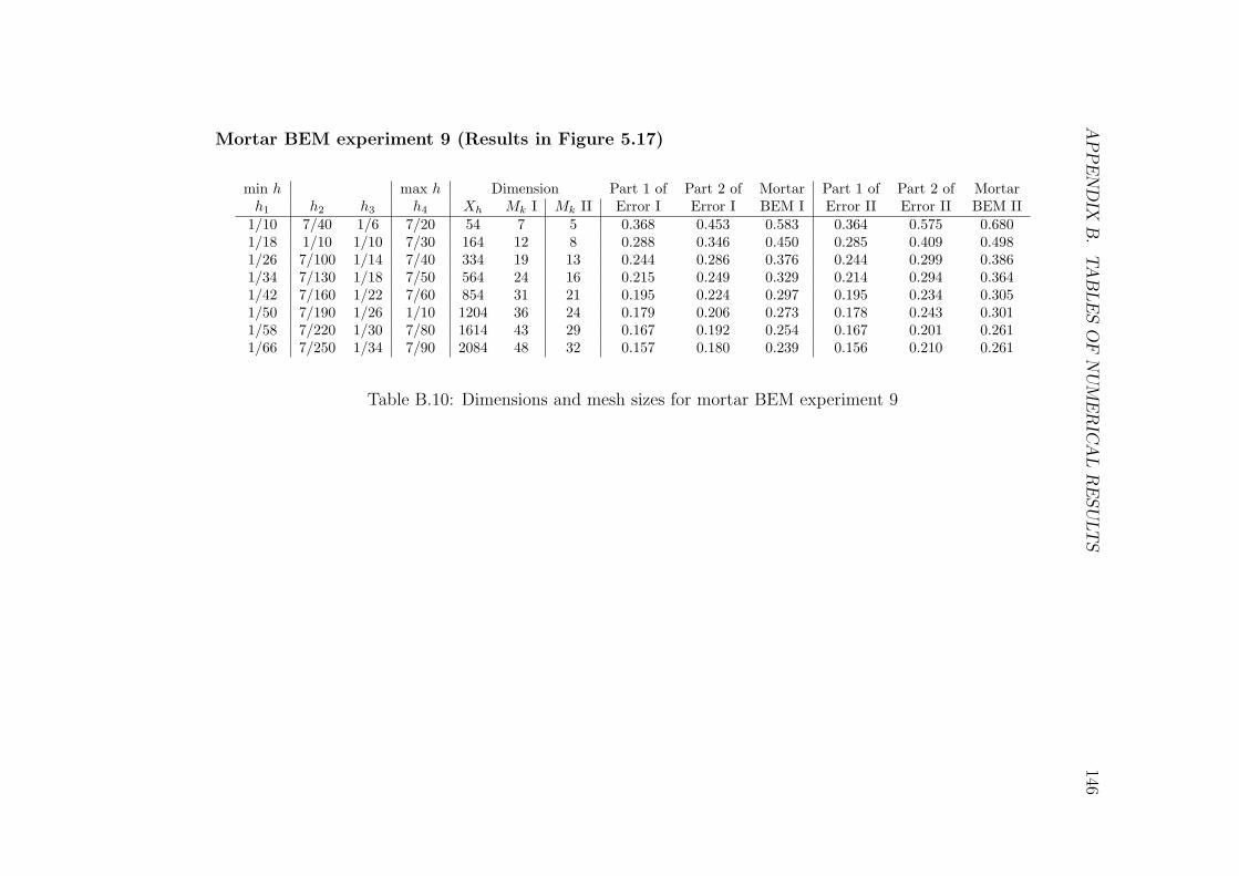
AP
PE
ND
IXB
.TA
BLE
SO
FN
UM
ER
ICA
LR
ESU
LT
S146
Mortar BEM experiment 9 (Results in Figure 5.17)
min h max h Dimension Part 1 of Part 2 of Mortar Part 1 of Part 2 of Mortarh1 h2 h3 h4 Xh Mk I Mk II Error I Error I BEM I Error II Error II BEM II
1/10 7/40 1/6 7/20 54 7 5 0.368 0.453 0.583 0.364 0.575 0.6801/18 1/10 1/10 7/30 164 12 8 0.288 0.346 0.450 0.285 0.409 0.4981/26 7/100 1/14 7/40 334 19 13 0.244 0.286 0.376 0.244 0.299 0.3861/34 7/130 1/18 7/50 564 24 16 0.215 0.249 0.329 0.214 0.294 0.3641/42 7/160 1/22 7/60 854 31 21 0.195 0.224 0.297 0.195 0.234 0.3051/50 7/190 1/26 1/10 1204 36 24 0.179 0.206 0.273 0.178 0.243 0.3011/58 7/220 1/30 7/80 1614 43 29 0.167 0.192 0.254 0.167 0.201 0.2611/66 7/250 1/34 7/90 2084 48 32 0.157 0.180 0.239 0.156 0.210 0.261
Table B.10: Dimensions and mesh sizes for mortar BEM experiment 9
Bibliography
[1] I. Babuska. The finite element method with Lagrangian multipliers. Numer. Math.,1972.
[2] I. Babuska and G. N. Gatica. On the mixed finite element method with Lagrangemultipliers. Numer. Methods Partial Differential Equation, 19:192–210, 2003.
[3] F. Ben Belgacem. The mortar finite element method with Lagrange multiplier. Nu-mer. Math., 84:173–197, 1999.
[4] F. Ben Belgacem and Y. Maday. The mortar finite element method for three dimen-sional finite elements. M2AN Math. Model. Numer. Anal., 31:289–302, 1997.
[5] C. Bernardi, Y. Maday, and A. T. Patera. Domain decomposition by the mortarelement method. In H. G. Karper and M. Garbey, editors, Asymptotic and Numericalmethods for partial differential equations with critical parameters, pages 269–286.Kluwer Academic Publishers, Netherlands, 1993.
[6] C. Bernardi, Y. Maday, and A. T. Patera. A new nonconforming approach to domaindecomposition: the mortar element method. In H. Brezis and J. L. Lions, editors,Nonlinear Partial Differential Equations and their Applications, pages 13–51. Pitman,New York, 1994.
[7] A. Bespalov and N. Heuer. The p-version of the boundary element method for athree-dimensional crack problem. Numer. Methods Partial Differential Eq., 19:243–258, 2003.
[8] A. Bespalov and N. Heuer. The hp-version of the boundary element method withquasi-uniform meshes in three dimensions. ESAIM Math. Model. Numer. Anal.,42(5):821–849, 2008.
[9] D. Braess. Finite Elements. Theory, fast solvers, and applications in solid mechanics.Cambridge University Press, Cambridge, 3rd edition, 2007.
147
BIBLIOGRAPHY 148
[10] D. Braess and W. Dahmen. Stability estimates of the mortar finite element methodfor 3-dimensional problems. East-West J. Numer. Math., 6:249–264, 1998.
[11] D. Braess, W. Dahmen, and C. Wieners. A multigrid algorithm for the mortar finiteelement method. SIAM J. Numer. Anal., 37:48–69, 1999.
[12] D. Braess, M. Dryja, and W. Hackbusch. A multigrid method for nonconformingfe-discretisations with application to nonmatching grids. Computing, 63:1–25, 199.
[13] S. C. Brenner. Poincare-Friedrichs inequalities for piecewise H1 functions. SIAM J.Numer. Anal., 41:306–324, 2003.
[14] S. C. Brenner and L. R. Scott. The Mathematical Theory of Finite Element Methods.Springer, New York, 2nd edition, 2002.
[15] A. Buffa, M. Costabel, and D. Sheen. On traces for H(curl,Ω) in Lipschitz domains.J. Math. Anal. Appl, 276:845–867, 2002.
[16] M. Cessenat. Mathematical methods in electromagnetism, volume 41 of Advances inMathematical Applied Science. World Scientific, Singapore, 1996.
[17] A. Chernov, M. Maischak, and E. P. Stephan. hp-mortar boundary element methodfor two-body contact problems with friction. Math. Methods Appl. Sci., 31:2029–2054,2008.
[18] P. G. Ciarlet. The finite element for elliptic problems. North-Holland, Amsterdam,1978.
[19] M. Costabel. Boundary integral operators on Lipschitz domains: Elementary results.SIAM J. Math. Anal., 19:613–626, 1988.
[20] W. Dahmen, B. Faermann, I. G. Graham, W. Hackbusch, and S. A. Sauter. In-verse inequalities on non-quasi-uniform meshes and application to the mortar elementmethod. Math. Comp, 73:1107–1138, 2004.
[21] M. R. Dorr. The approximation theory for the p-version of the finite element method.SIAM J. Numer. Anal., 21:1180–1207, 1984.
[22] K. Eriksson, D. Estep, P. Hansbro, and C. Johnson. Computational DifferentialEquations. Cambridge University Press, Cambridge, 1996.
[23] V.J. Ervin, N. Heuer, and E.P. Stephan. On the h-p version of the boundary elementmethod for Symm’s integral equation on polygons. Comput. Methods Appl. Mech.Engrg., 110:25–38, 1993.

BIBLIOGRAPHY 149
[24] G. I. Eskin. Boundary value problems for elliptic pseuddifferential equations, vol-ume 52 of Translations of Mathematical Monographs. American Mathematical Soci-ety, Providence, RI, 1981.
[25] G. Gatica, M. Healey, and N. Heuer. The boundary element method with Lagrangianmultipliers. Numer. Methods Partial Differential Eq., 25(6):1303–1341, 2009.
[26] P. Grisvard. Elliptic Problems in Nonsmooth Domains. Pitman Publishing Inc.,Boston, 1985.
[27] H. Han. The boundary integro-differential equations of three-dimensional Neumannproblem in linear elasticity. Numer. Math., 68:269–281, 1994.
[28] M. Healey and N. Heuer. Mortar boundary elements. arxiv:0901.4960, 2009.
[29] N. Heuer. Additive Schwarz method for the p-version of the boundary element methodfor the single layer potential on a plane screen. Numer. Math., 88:485–511, 2001.
[30] N. Heuer and FJ. Sayas. Crouzeix-Raviart boundary elements. Numer. Math.,112(3):381–401, 2009.
[31] G. C. Hsiao and W. L. Wendland. A finite element method for some integral equationsof the first kind. J. Math. Anal. Appl., 58:449–481, 1977.
[32] G. C. Hsiao and W. L. Wendland. Boundary Integral Equations. Springer, Berlin,2008.
[33] G. C. Hsiao and W. L. Wendland. The hp-version of the boundary element methodwith quasi-uniform meshes in three dimensions. ESAIM Math. Model. Numer. Anal.,42:821–849, 2008.
[34] C. Johnson. Numerical solution of partial differential equations by the finite elementmethod. Cambridge University Press, Cambridge, 1987.
[35] C. Kim, R. D. Lazarov, J. E. Pasciak, and P. S. Vassilevski. Multiplier spaces forthe finite element method in three dimensions. SIAM J. Numer. Anal., 39:519–538,2001.
[36] A. Klawonn and O. B. Widlund. A domain decomposition method with Lagrangemultipliers andd inexact solvers for linear elasticity. SIAM J. Sci. Comput., 22:1199–1219, 2000.
[37] V.D. Kupradze. Three-dimensional problems of the mathematical theory of elasticityand thermoelasticity. North-Holland, Amsterdam, 1979.
BIBLIOGRAPHY 150
[38] J. L. Lions and E. Magenes. Non-Homogeneous Boundary Value Problems and Ap-plications I. Springer-Verlag, New York, 1972.
[39] M. Maischak. The analytical computation of the Galerkin elements for the Laplace,Lame, and Helmholtz equation in 3D-BEM. Report, Institute fur Angewandte Math-ematik, University of Hannover, Germany, 2000.
[40] A.-W. Maue. Zur formulierung eines allgemeinen beugungsproblems durch eine in-tegralgleichung. Zeitschrift fur Physik, 126:601–618, 1949.
[41] W. McLean. Strongly Elliptic Systems and Boundary Integral Equations. CambridgeUniversity Press, Cambridge, 2000.
[42] S. E. Mikhailov. About traces, extensions and co-normal derivative operators onLipschitz domains. In C. Constanda and S. Potapenko, editors, Integral methodsin science and engineering: techniques and applications, pages 151–162. Birkhauser,Boston, 2007.
[43] J.-C. Nedelec. Integral equations with nonintegrable kernels. Integral EquationsOperator Theory, 5:562–572, 1982.
[44] J.-C. Nedelec and J. Planchard. Une methode variationnelle d’elements finis pour laresolution numerique d’un probleme exteriieur dans R3. RAIRO, 7:105–129, 1973.
[45] A. Patel, A. K. Pani, and N. Nataraj. Mortar element methods for parabolic prob-lems. Numer. Methods Partial Differential Eq., 24:1460–1484, 2008.
[46] A. Quateroni and A. Valli. Domain Decomposition Methods for Partial DifferentialEquations. Oxford University Press, Oxford, 1999.
[47] P. A. Raviart and J. M. Thomas. Primal hybrid finite element methods for 2nd orderelliptic equations. Math. Comp., 31:391–413, 1977.
[48] J. E. Roberts and J. M. Thomas. Mixed and hybrid methods (in finite elementsproblems). In P. G. Ciarlet and J. L. Lions, editors, Handbook of numerical analysis,volume 2, pages 523, 525–639. North-Holland, Amsterdam, 1991.
[49] F.J. Sayas. Infimum-supremum. Boletin SEMA, 41, 2007.
[50] P. Seshaiyer and M. Suri. Uniform hp convergence results for the mortar finite elementmethod. Math. Comp., 69:521–546, 2000.
[51] O. Steinbach. Numerical Approximation Methods for Elliptic Boundary Value Prob-lems. Springer Science+Business Media, LLC, New York, 2008.
BIBLIOGRAPHY 151
[52] E. P. Stephan. A boundary integral equation method for three-dimensional crackproblems in elasticity. Math. Meth. in the Appl. Sci., 8:609–623, 1986.
[53] E. P. Stephan. Boundary integral equations for screen problems in R3. IntegralEquations Operator Theory, 10:257–263, 1987.
[54] A. Toselli and O. Widlund. Domain Decomposition Methods - algorithms and theory.Springer-Verlag, Berlin, 2005.
[55] T. von Petersdorff and E. P. Stephan. Decompositions in edge and corner singularitiesfor the solution of the Dirichlet problem of the Laplacian in a polyhedron. Math.Nachr., 149:71–104, 1990.
[56] T. von Petersdorff and E. P. Stephan. Regularity of mixed boundary value problemsin R3 and boundary element methods on graded meshes. Math. Methods Appl. Sci.,12:229–249, 1990.
[57] B. Wohlmuth. Hierarchical a posteriori error estimators for mortar finite elementmethods with Lagrange multipliers. SIAM J. Numer. Anal., 36:1636–1658, 1999.
[58] B. I. Wohlmuth. A mortar finite element method using dual spaces for the Lagrangianmultiplier. SIAM J. Numer. Anal., 38:989–1012, 2000.
Index
Babuska-Brezzi theoryContinuous, 18Discrete, 18
Cea’s lemma, 12Continuous bilinear form, 12Continuous linear form, 12
Discrete formulationBEM, 11
Elliptic bilinear form, 12
FEM with Lagrangian multiplier, 17Finite element method, 14First Green formula, 14Fractional order Sobolev norm, 9Fundamental solution
Linear elasticity, 101
Gunter derivatives, 104Geometrical conforming decomposition, 50
Hypersingular integral equationLaplacian, 10Linear elasticity, 102
Interface, 51Interface edges, 52
Lagrangian multiplier, 16Lagrangian multiplier side, 52Lame constants, 100Lax-Milgram Theorem, 12
Mesh, 11Mesh size, 11Mortar boundary element method, 61
Linear elasticity, 114Mortar finite element method
Continuous formulation, 22Discrete formulation, 24
Mortar side, 52
Neumann problemLinear elasticity, 100Screen surface, 9
Poisson equation, 13
Quasi-optimal, 4
Rigid body motions, 101
Second Strang lemma, 15Single layer potential, 30
Linear elasticity, 113Sobolev spaces, 7Stokes Theorem, 107Strain tensor, 100Strang-type estimate, 20Stress operator, 100
Trace theorem, 32
Variational formulationBEM, 10Linear elasticity, 103
152